Real-time or full-precision CRS imaging using a cloud computing portal: multi-

offset GPR and SH-wave examples

Z. Heilmann*, H.P. Müller**, G. Satta* and G.P. Deidda***

*CRS4, Energy and Environment Sector

**ABE-geo, Burgdorf, Germany

***University of Cagliari, Department of Civil and Environmental Engineering, and Architecture

1

Outline

Part 1: Cloud computing portal

o Concept & Realization

o GPR example (Real-time imaging)

Part 2: CRS stack imaging

o from CMP to CRS stack

o 3x1 vs. 1x3 parameter search

o SH-wave data (Full-precision imaging)

Conclusions 2

3

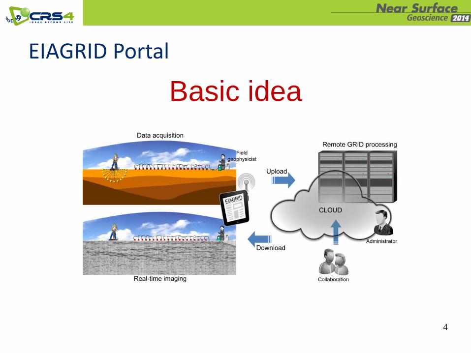
Basic idea

4

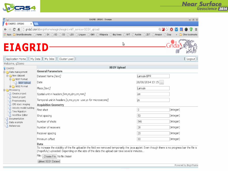
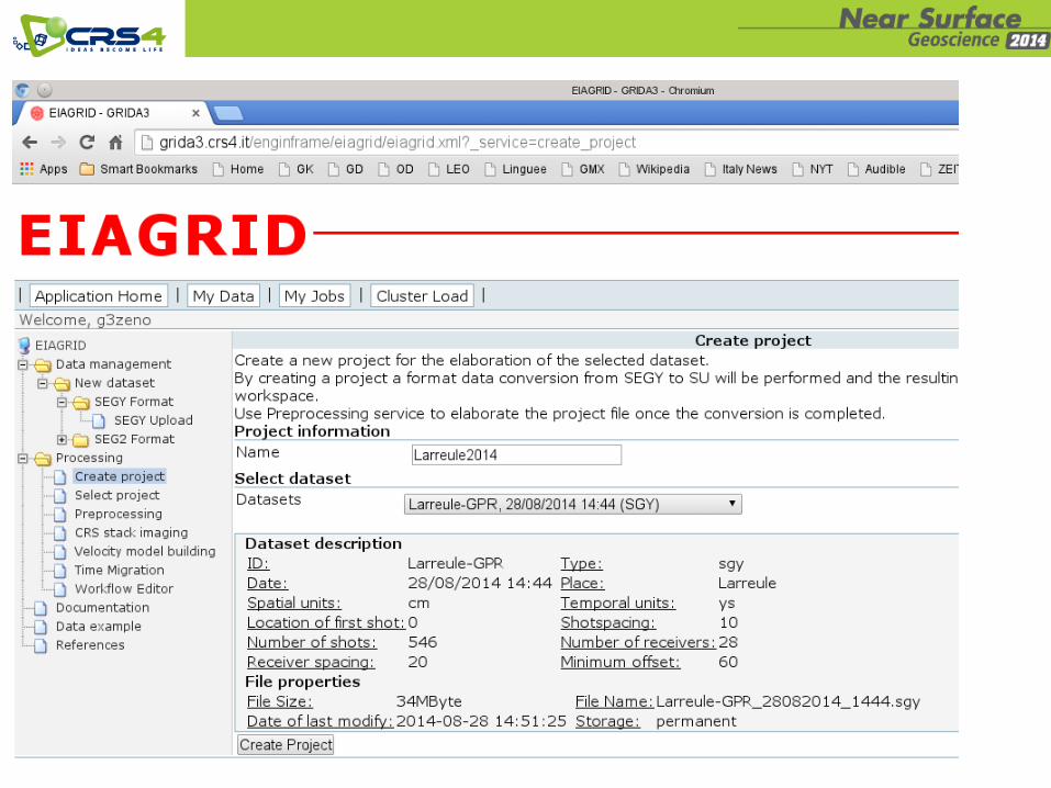
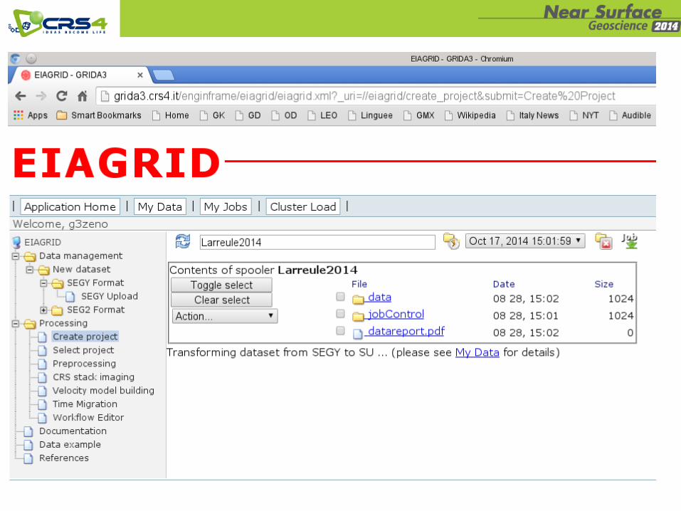
EIAGRID Portal

5

EIAGRID Portal

Basic idea

1. Web-browser-based interface accessible from the field

2. Real-time processing using distant HPC resources

3. Remote collaboration and acquisition controlling

Features

6

EIAGRID Portal

Basic idea

1. Project, data and user management

2. Simplistic toolbox for data visualization and manipulation

3. Data-driven imaging method suited for parallel computing

Components

7

Multi-offset GPR data:

8

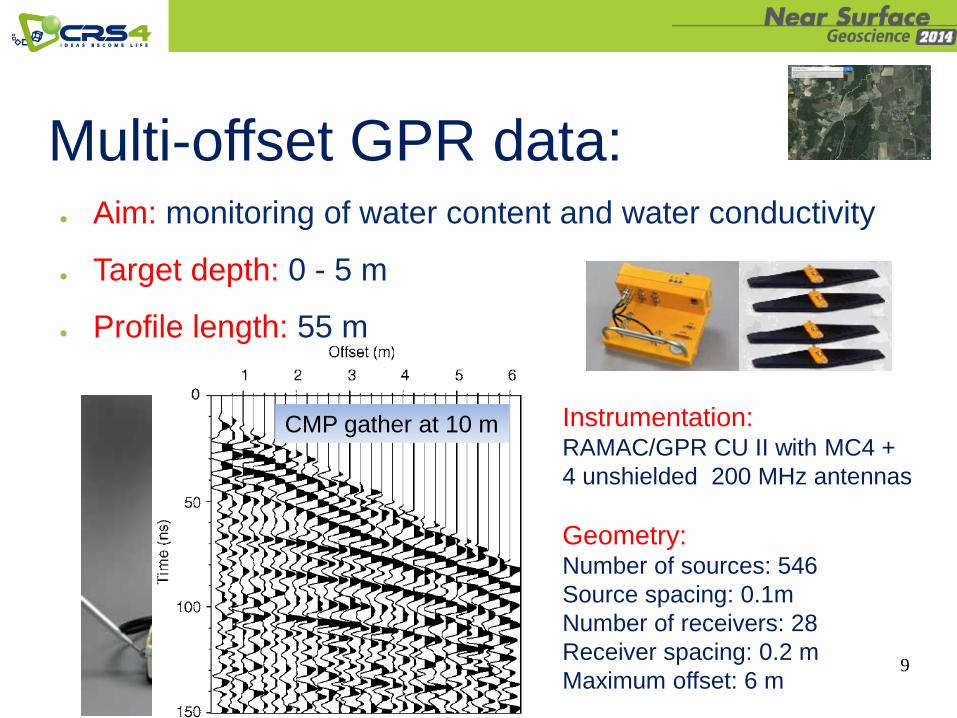
Multi-offset GPR data: ● Aim: monitoring of water content and water conductivity

● Target depth: 0 - 5 m

● Profile length: 55 m

Instrumentation: RAMAC/GPR CU II with MC4 +

4 unshielded 200 MHz antennas

Geometry: Number of sources: 546

Source spacing: 0.1m

Number of receivers: 28

Receiver spacing: 0.2 m

Maximum offset: 6 m 9

CMP gather at 10 m

Data visualization tools

Data visualization tools

Data visualization tools

Data visualization tools

cm/µs

cm/µs

cm/µs

MHz

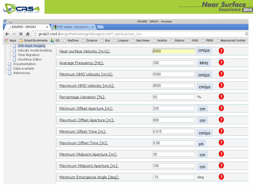
Data visualization tools

MHz

cm/µs

cm/µs

cm/µs

cm/µs

cm

cm

cm

cm

µs

CRS stacking result obtained after 4 minutes using 50 CPU

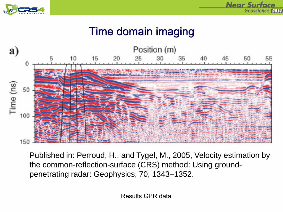
Time domain imaging

Published in: Perroud, H., and Tygel, M., 2005, Velocity estimation by

the common-reflection-surface (CRS) method: Using ground-

penetrating radar: Geophysics, 70, 1343–1352.

Results GPR data

GPR data

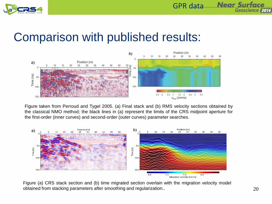
Comparison with published results:

Figure (a) CRS stack section and (b) time migrated section overlain with the migration velocity model

obtained from stacking parameters after smoothing and regularization.. 20

Figure taken from Perroud and Tygel 2005. (a) Final stack and (b) RMS velocity sections obtained by

the classical NMO method; the black lines in (a) represent the limits of the CRS midpoint aperture for

the first-order (inner curves) and second-order (outer curves) parameter searches.

21

From CMP to CRS stacking:

Figure taken from Perroud and Tygel 2005. NMO velocity analysis for the CMP at position x = 10 m.

22

Conventional CMP-by-CMP velocity analysis:

𝑡𝐶𝑀𝑃2 ℎ = 𝑡0

2 +4ℎ2

𝑣𝑁𝑀𝑂2

CRS stacking operator:

Hyperbolic traveltime in CRS gather:

𝑡𝐶𝑅𝑆2 ∆𝑥𝑚, ℎ = 𝑡0 +

2 sin 𝛼

𝑣0∆𝑥𝑚

2

+2𝑡0 cos2 𝛼

𝑣0

∆𝑥𝑚2

𝑅𝑁+

ℎ2

𝑅𝑁𝐼𝑃,

𝑤𝑖𝑡ℎ ∆𝑥𝑚 = 𝑥𝑚 − 𝑥0.

… in CMP gather:

𝑡𝐶𝑀𝑃2 ℎ = 𝑡0

2 +4ℎ2

𝑣𝑁𝑀𝑂2

𝑤𝑖𝑡ℎ 𝑣𝑁𝑀𝑂2 =

2𝑣0𝑅𝑁𝐼𝑃

𝑡0 cos2 𝛼

Fig.: Mann et al. 2007

24

Stacking parameter search:

Pragmatic search: 3 x 1 parameter line search in specific

gathers (Mann et al. 1999) + Cloud = Real-time imaging

One step search:

1 x 3 parameter surface search in

prestack data (Garabito et al. 2001)

+ Cloud = High-precision imaging

Figs: Mann et al. 2007

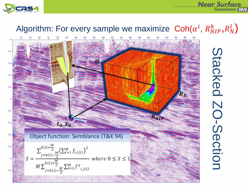
Algorithm: For every sample we maximize Coh(𝛼𝑖, 𝑅𝑁𝐼𝑃𝑘 ,𝑅𝑁

𝑙 )

● Sta

cked Z

O-S

ectio

n

𝑹𝑵𝑰𝑷

𝑹𝑵

Object function: Semblance (T&K 94)

𝒕𝟎, 𝒙𝟎

Shallow SH-data:

26

Shallow SH-data:

27

28

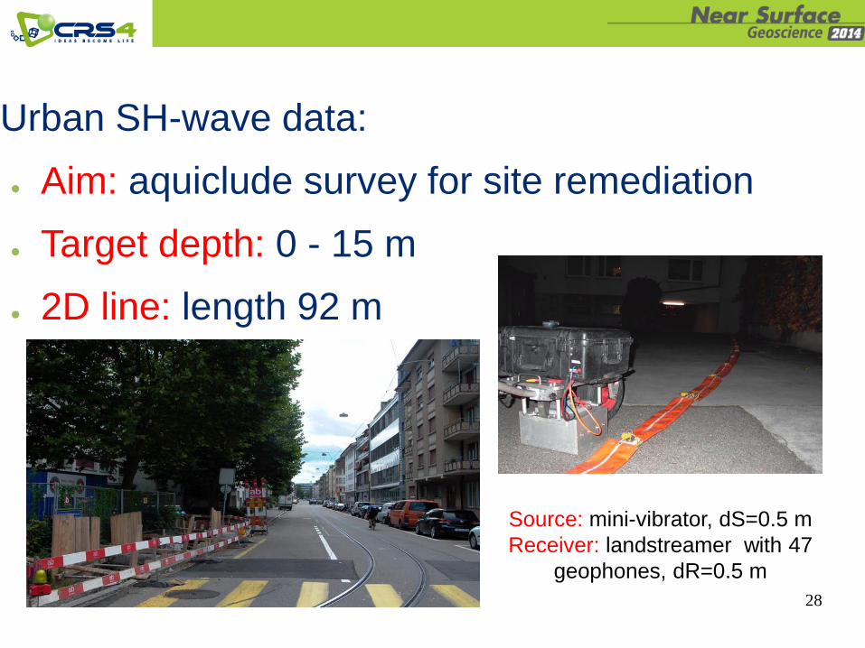
Urban SH-wave data:

● Aim: aquiclude survey for site remediation

● Target depth: 0 - 15 m

● 2D line: length 92 m

Source: mini-vibrator, dS=0.5 m

Receiver: landstreamer with 47

geophones, dR=0.5 m

29

Some CMP gathers:

CMP 1171 CMP 1267 CMP 1069

Offset [dm] Offset [dm] Offset [dm]

Tim

e [m

s]

Tim

e [m

s]

Tim

e [m

s]

30

Stacking results:

CMP stack after CVS analysis (a) versus 3x1 parameter CRS stack (b)

a)

b)

+ higher S/N

- unresolved events

31

Stacking results:

CMP stack after CVS analysis (a), 3x1 parameter search CRS stack (b)

a)

b)

32

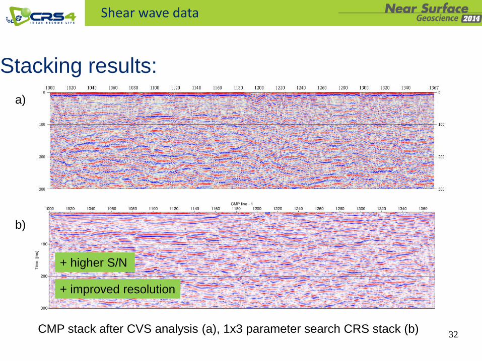
Shear wave data

Stacking results:

CMP stack after CVS analysis (a), 1x3 parameter search CRS stack (b)

a)

b)

+ higher S/N

+ improved resolution

Computational cost:

0 50 100

3x1 Parameter

2-Parameter

3-Parameter

submission-time[min] on 30 CPU

runtime [min] on30 CPUs

34

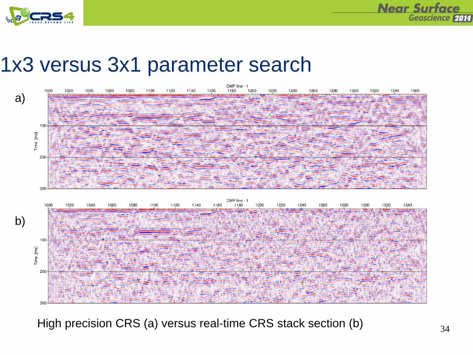
1x3 versus 3x1 parameter search

High precision CRS (a) versus real-time CRS stack section (b)

a)

b)

35

Shear wave data

1x3 versus 3x1 parameter search

NMO velocities calculated using 𝑅𝑁𝐼𝑃 and 𝛼: High precision CRS (a) versus

real-time CRS stack section (b)

a)

b)

36

Outlook: Depth imaging

(a) Velocity model from inversion of 𝑅𝑁𝐼𝑃 and 𝛼, (b) PostSDM

a)

b)

37

Outlook: Depth imaging

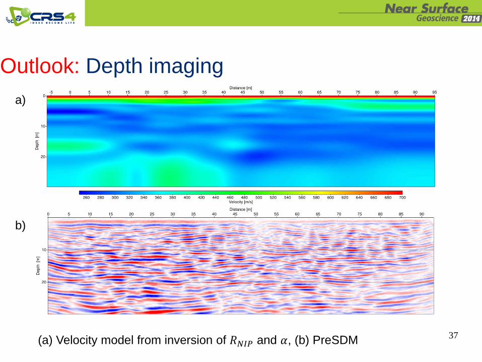
(a) Velocity model from inversion of 𝑅𝑁𝐼𝑃 and 𝛼, (b) PreSDM

a)

b)

38

Outlook: Depth migration

(a) PreSDM (b) PostSDM using Dix inversion of CVS velocity

a)

b)

Top of Molasse

VSP

39

Conclusions:

• Real-time CRS imaging can be applied to optimize crutial acquisition parameters directly in the field:

easier use of reflection methods in near-surface.

• Full-precision CRS imaging uses a spatial operator not only for stacking but also for velocity analysis:

higher resolution and more stable velocities in case of low fold, strong noise & lateral inhomogeneity.

• A cloud computing portal provides optimum computing power in a location independent way:

reduced hardware requirement facilitate the use of data driven methods in near-surface imaging.

Thank you for your attention!

40

Stacking parameter search:

# coh. calculated:

Full parameter search: Optimizing 1 x 3 parameters using entire data

C1 x C2 x C3

Pragmatic search: Optimizing 3 x 1 parameter in data subsets

C1

C3

C2

+

+

𝑥𝑚 = 𝑥0

CMP stack

ℎ = 0

𝑅𝑁 = 0

ℎ = 0