Accepted for publication in the Astrophysical Journal

Kepler-1647b: the largest and longest-period Kepler transiting circumbinaryplanet.

Veselin B. Kostov1,25, Jerome A. Orosz2, William F. Welsh2, Laurance R. Doyle3,Daniel C. Fabrycky4, Nader Haghighipour5, Billy Quarles6,7,25, Donald R. Short2,

William D. Cochran8, Michael Endl8, Eric B. Ford9, Joao Gregorio10, Tobias C. Hinse11,12,Howard Isaacson13, Jon M. Jenkins14, Eric L. N. Jensen15, Stephen Kane16, Ilya Kull17,

David W. Latham18, Jack J. Lissauer14, Geoffrey W. Marcy13, Tsevi Mazeh17,Tobias W. A. Muller19, Joshua Pepper20, Samuel N. Quinn21,26, Darin Ragozzine22,

Avi Shporer23,27, Jason H. Steffen24, Guillermo Torres18, Gur Windmiller2, William J. Borucki14

veselin.b.kostov@nasa.gov

arX

iv:1

512.

0018

9v2

[as

tro-

ph.E

P] 1

9 M

ay 2

016

– 2 –

1NASA Goddard Space Flight Center, Mail Code 665, Greenbelt, MD, 20771

2Department of Astronomy, San Diego State University, 5500 Campanile Drive, San Diego, CA 92182

3SETI Institute, 189 Bernardo Avenue, Mountain View, CA 94043; and Principia College, IMoP, One MaybeckPlace, Elsah, Illinois 62028

4Department of Astronomy and Astrophysics, University of Chicago, 5640 South Ellis Avenue, Chicago, IL 60637

5Institute for Astronomy, University of Hawaii-Manoa, Honolulu, HI 96822, USA

6Department of Physics and Physical Science, The University of Nebraska at Kearney, Kearney, NE 68849

7NASA Ames Research Center, Space Science Division MS 245-3, Code SST, Moffett Field, CA 94035

8McDonald Observatory, The University of Texas as Austin, Austin, TX 78712-0259

9Department of Astronomy and Astrophysics, The Pennsylvania State University, 428A Davey Lab, UniversityPark, PA 16802, USA

10Atalaia Group and Crow-Observatory, Portalegre, Portugal

11Korea Astronomy and Space Science Institute (KASI), Advanced Astronomy and Space Science Division, Dae-jeon 305-348, Republic of Korea

12Armagh Observatory, College Hill, BT61 9DG Armagh, Northern Ireland, UK

13Department of Astronomy, University of California Berkeley, 501 Campbell Hall, Berkeley, CA 94720, USA

14NASA Ames Research Center, Moffett Field, CA 94035, USA

15Department of Physics and Astronomy, Swarthmore College, Swarthmore, PA 19081, USA

16Department of Physics and Astronomy, San Francisco State University, 1600 Holloway Avenue, San Francisco,CA 94132, USA

17Department of Astronomy and Astrophysics, Tel Aviv University, 69978 Tel Aviv, Israel

18Harvard-Smithsonian Center for Astrophysics, 60 Garden Street, Cambridge, MA 02138

19Institute for Astronomy and Astrophysics, University of Tuebingen, Auf der Morgenstelle 10, D-72076 Tuebin-gen, Germany

20Department of Physics, Lehigh University, Bethlehem, PA 18015, USA

21Department of Physics and Astronomy, Georgia State University, 25 Park Place NE Suite 600, Atlanta, GA 30303

22Department of Physics and Space Sciences, Florida Institute of Technology, 150 W. University Blvd, Melbourne,FL 32901, USA

23Jet Propulsion Laboratory, California Institute of Technology, 4800 Oak Grove Drive, Pasadena, CA 91109, USA

24Department of Physics and Astronomy, Northwestern University, 2145 Sheridan Road, Evanston, IL 60208

25NASA Postdoctoral Fellow

26NSF Graduate Research Fellow

– 3 –

ABSTRACT

We report the discovery of a new Kepler transiting circumbinary planet (CBP).This latest addition to the still-small family of CBPs defies the current trend of knownshort-period planets orbiting near the stability limit of binary stars. Unlike the previousdiscoveries, the planet revolving around the eclipsing binary system Kepler-1647 hasa very long orbital period (∼ 1100 days) and was at conjunction only twice duringthe Kepler mission lifetime. Due to the singular configuration of the system, Kepler-1647b is not only the longest-period transiting CBP at the time of writing, but also oneof the longest-period transiting planets. With a radius of 1.06±0.01 RJup it is also thelargest CBP to date. The planet produced three transits in the light-curve of Kepler-1647 (one of them during an eclipse, creating a syzygy) and measurably perturbed thetimes of the stellar eclipses, allowing us to measure its mass to be 1.52± 0.65 MJup.The planet revolves around an 11-day period eclipsing binary consisting of two Solar-mass stars on a slightly inclined, mildly eccentric (ebin = 0.16), spin-synchronizedorbit. Despite having an orbital period three times longer than Earth’s, Kepler-1647b isin the conservative habitable zone of the binary star throughout its orbit.

Subject headings: binaries: eclipsing – planetary systems – stars: individual (KIC-5473556, KOI-2939, Kepler-1647) – techniques: photometric

1. Introduction

Planets with more than one sun have long captivated our collective imagination, yet directevidence of their existence has emerged only in the past few years. Eclipsing binaries, in par-ticular, have long been thought of as ideal targets to search for such planets (Borucki & Sum-mers 1984, Schneider & Chevreton 1990, Schneider & Doyle 1995, Jenkins et al. 1996, Deeget al. 1998). Early efforts to detect transits of a circumbinary planet around the eclipsing binarysystem CM Draconis—a particularly well-suited system composed of two M-dwarfs on a nearlyedge-on orbit—suffered from incomplete temporal coverage (Schneider & Doyle 1995, Doyle etal. 2000, Doyle & Deeg 2004). Several non-transiting circumbinary candidates have been pro-posed since 2003, based on measured timing variations in binary stellar systems (e.g., Zorotovic& Schreiber 2013). The true nature of these candidates remains, however, uncertain and rigorousdynamical analysis has challenged the stability of some of the proposed systems (e.g., Hinse et

27Sagan Fellow

– 4 –

al. 2014, Schleicher et al. 2015). It was not until 2011 and the continuous monitoring of thousandsof eclipsing binaries (hereafter EBs) provided by NASA’s Kepler mission that the first circumbi-nary planet, Kepler-16b, was unambiguously detected through its transits (Doyle et al. 2011).Today, data from the mission has allowed us to confirm the existence of 10 transiting circumbi-nary planets in 8 eclipsing binary systems (Doyle et al. 2011, Welsh et al. 2012, 2015, Orosz etal. 2012ab, 2015, Kostov et al. 2013, 2014, Schwamb et al. 2013). Curiously enough, these plan-ets have all been found to orbit EBs from the long-period part of the Kepler EB distribution, andhave orbits near the critical orbital separation for dynamical stability (Welsh et al. 2014, Martin etal. 2015).

These exciting new discoveries provide better understanding of the formation and evolutionof planets in multiple stellar system, and deliver key observational tests for theoretical predic-tions (e.g., Paardekooper et al. 2012, Rafikov 2013, Marzari et al. 2013, Pelupessy & PortegiesZwart 2013, Meschiari 2014, Bromley & Kenyon 2015, Silsbee & Rafikov 2015, Lines et al. 2015,Chavez et al. 2015, Kley & Haghighipour 2014, 2015, Miranda & Lai 2015). Specifically, numer-ical simulations indicate that CBPs should be common, typically smaller than Jupiter, and close tothe critical limit for dynamical stability – due to orbital migration of the planet towards the edge ofthe precursor disk cavity surrounding the binary star (Pierens & Nelson, 2007, 2008, 2015, here-after PN07, PN08, PN15). Additionally, the planets should be co-planar (within a few degrees) forbinary stars with sub-AU separation due to disk-binary alignment on precession timescales (Fou-cart & Lai 2013, 2014). The orbital separation of each new CBP discovery, for example, constrainsthe models of protoplanetary disks and migration history and allow us to discern between an obser-vational bias or a migration pile-up (Kley & Haghighipour 2014, 2015). Discoveries of misalignedtransiting CBPs such as Kepler-413b (Kostov et al. 2014) and Kepler-453b (Welsh et al. 2015)help determine the occurrence frequency of CBPs by arguing for the inclusion of a distributionof possible planetary inclinations into abundance estimates (Schneider 1994; Kostov et al. 2014;Armstrong et al. 2014, Martin & Triaud 2014).

In terms of stellar astrophysics, the transiting CBPs provide excellent measurements of thesizes and masses of their stellar hosts, and can notably contribute towards addressing a knowntension between the predicted and observed characteristics of low-mass stars, where the stellarmodels predict smaller (and hotter) stars than observed (Torres et al. 2010, Boyajian et al. 2012, butalso see Tal-Or et al. 2013). Each additional CBP discovery sheds new light on the still-uncertainmechanism for the formation of close binary systems (Tohline 2002). For example, the lack ofCBPs around a short-period binary star (period less than ∼ 7 days) lends additional support for acommonly favored binary formation scenario of a distant stellar companion driving tidal frictionand Kozai-Lidov circularization of the initially wide host binary star towards its current closeconfiguration (Kozai 1962; Lidov 1962; Mazeh & Shaham 1979, Fabrycky & Tremaine 2007,Martin et al. 2015, Munoz & Lai 2015, Hamers et al. 2015).

– 5 –

Here we present the discovery of the Jupiter-size transiting CBP Kepler-1647b that orbits its11.2588-day host EB every∼1,100 days – the longest-period transiting CBP at the time of writing.The planet completed a single revolution around its binary host during Kepler’s data collection andwas at inferior conjunction only twice – at the very beginning of the mission (Quarter 1) and againat the end of Quarter 13. The planet transited the secondary star during the same conjunction andboth the primary and secondary stars during the second conjunction.

The first transit of the CBP Kepler-1647b was identified and reported in Welsh et al. (2012);the target was subsequently scheduled for short cadence observations as a transiting CBP candidate(Quarters 13 through 17). At the time, however, this single event was not sufficient to rule outcontamination from a background star or confirm the nature of the signal as a transit of a CBP. AsKepler continued observing, the CBP produced a second transit – with duration and depth notablydifferent from the first transit – suggesting a planet on either ∼550-days or ∼1,100-days orbit.The degeneracy stemmed from a gap in the data where a planet on the former orbit could havetransited (e.g., Welsh et al. 2014, Armstrong et al. 2014). After careful visual inspection of theKepler light-curve, we discovered another transit, heavily blended with a primary stellar eclipse afew days before the second transit across the secondary star. As discussed below, the detection ofthis blended transit allowed us to constrain the period and pin down the orbital configuration of theCBP – both analytically and numerically.

This paper is organized as follows. We describe our analysis of the Kepler data (Section 2)and present our photometric and spectroscopic observations of the target (Section 3). Section 4details our analytical and photometric-dynamical characterization of the CB system, and outlinesthe orbital dynamics and long-term stability of the planet. We summarize and discuss our resultsin Section 5 and draw conclusions in Section 6.

2. Kepler Data

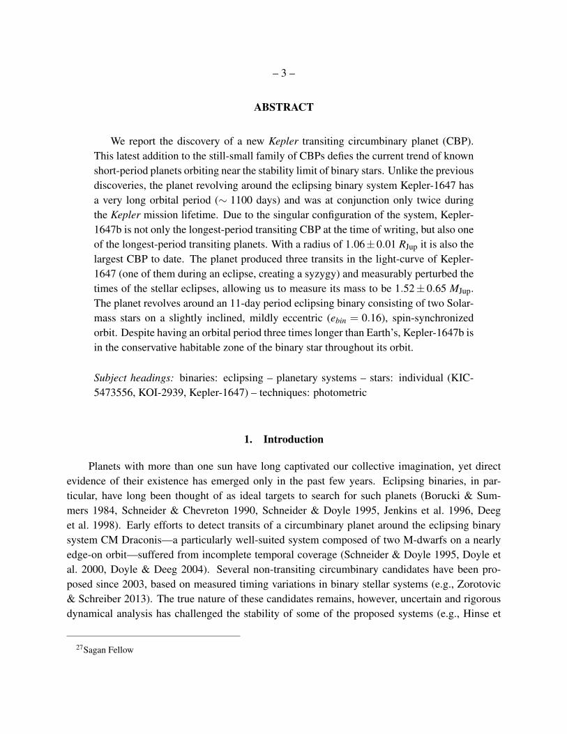
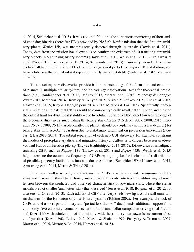
Kepler-1647 is listed in the NExScI Exoplanet Archive as a 11.2588-day period eclipsingbinary with a Kepler magnitude of 13.545. It has an estimated effective temperature of 6217K,surface gravity logg of 4.052, metallicity of -0.78, and primary radius of 1.464 R. The target isclassified as a detached eclipsing binary in the Kepler EB Catalog, with a morphology parameterc = 0.21 (Prsa et al. 2011, Slawson et al. 2011, Matijevic et al. 2012, Kirk et al. 2015). The light-curve of Kepler-1647 exhibits well-defined primary and secondary stellar eclipses with depths of∼ 20% and ∼ 17% respectively, separated by 0.5526 in phase (see Kepler EB Catalog). A sectionof the raw (SAPFLUX) Kepler light-curve of the target, containing the prominent stellar eclipsesand the first CBP transit, is shown in the upper panel of Figure 1.

– 6 –

Fig. 1.— Upper panel: A representative section of the raw (SAPFLUX), long-cadence light-curveof Kepler-1647 (black symbols) exhibiting two primary, three secondary stellar eclipses, and thefirst transit of the CBP. Lower panel: Same, but with the stellar eclipses removed and zoomed-into show the ∼ 11−days out-of eclipse modulation. This represents the end of Quarter 1, which isfollowed by a few days long data gap. Note the differences in scale between the two panels.

– 7 –

2.1. Stellar Eclipses

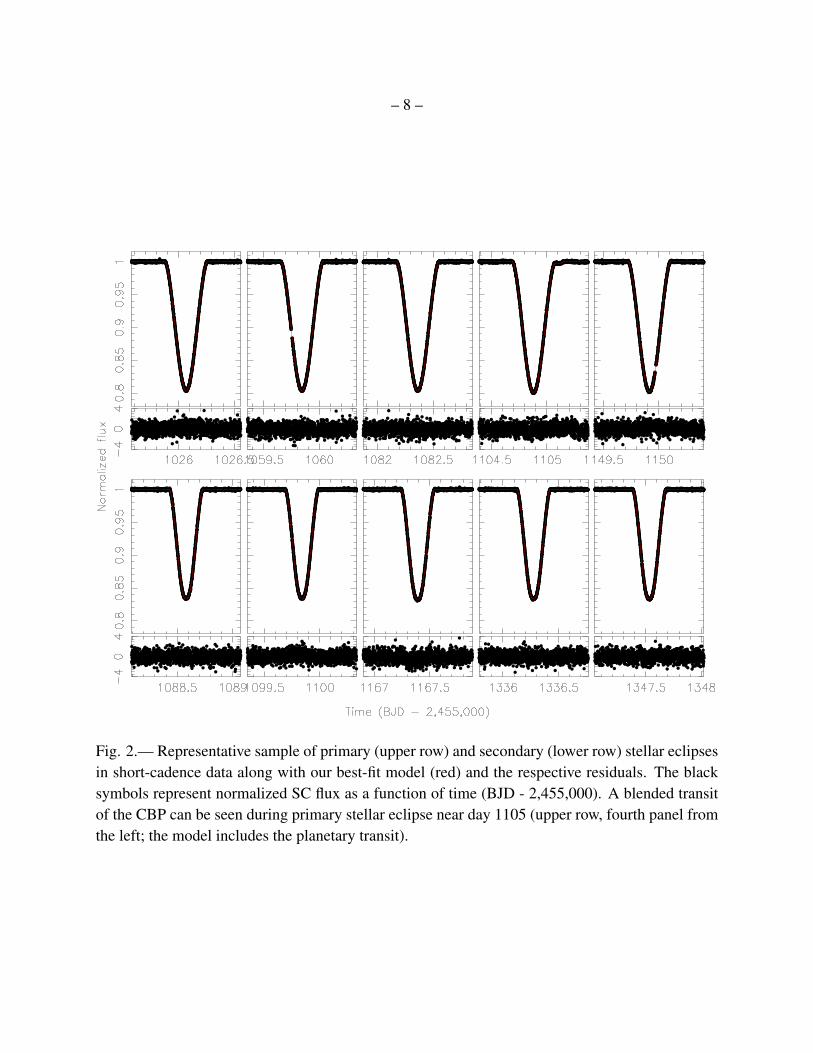
The information contained in the light-curve of Kepler-1647 allowed us to measure the orbitalperiod of the EB and obtain the timing of the stellar eclipse centers (Tprim, Tsec), the flux and radiusratio between the two stars (FB/FA and RB/RA), the inclination of the binary (ibin), and the nor-malized stellar semi-major axes (RA/abin, RB/abin) as follows.1 First, we extracted sub-sections ofthe light-curve containing the stellar eclipses and the planetary transits. We only kept data pointswith quality flags less than 16 (see Kepler user manual) – the rest were removed prior to our anal-ysis. Next, we clipped out each eclipse, fit a 5th-order Legendre polynomial to the out-of-eclipsesection only, then restored the eclipse and normalize to unity. Finally, we modeled the detrended,normalized and phase-folded light-curve using the ELC code (Orosz & Hauschildt 2000, Welsh etal. 2015). A representative sample of short-cadence (SC) primary and secondary stellar eclipses,along with our best-fit model and the respective residuals, are shown in Figure 2.

To measure the individual mid-eclipse times, we first created an eclipse template by fitting aMandel & Agol (2002) model to the phase-folded light-curve for both the primary and secondarystellar eclipses. We carefully chose five primary and secondary eclipses (see Figure 2) where thecontamination from spot activity – discussed below – is minimal. Next, we slid the template acrossthe light-curve, iteratively fitting it to each eclipse by adjusting only the center time of the templatewhile kepting the EB period constant. The results of the SC and LC data analysis were mergedwith preference given to the SC data.

We further used the measured primary and secondary eclipse times to calculate eclipse timevariations (ETVs). These are defined in terms of the deviations of the center times of each eclipsefrom a linear ephemeris fit through all primary and all secondary mid-eclipse times, respectively(for a common binary period).

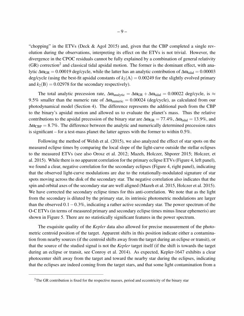
The respective primary and secondary “Common Period Observed minus Calculated” (CPOC,or O-C for short) measurements are shown in Figure 3. The 1σ uncertainty is ∼ 0.1 min for themeasured primary eclipses, and∼ 0.14 min for the measured secondary eclipses. As seen from thefigure, the divergence in the CPOC is significantly larger than the uncertainties.

The measured Common Period Observed minus Calculated (CPOC) are a key ingredient inestimating the mass of the CBP. As in the case of Kepler-16b, Kepler-34b and Kepler-35b (Doyleet al. 2011, Welsh et al. 2012), the gravitational perturbation of Kepler-1647b imprints a detectablesignature on the measured ETVs of the host EB – indicated by the divergent primary (black sym-bols) and secondary (red symbols) CPOCs shown in Figure 3. We note that there is no detectable

1Throughout this paper we refer to the binary with a subscript “bin”, to the primary and secondary stars withsubscripts “A” and “B” respectively, and to the CBP with a subscript “p”.

– 8 –

Fig. 2.— Representative sample of primary (upper row) and secondary (lower row) stellar eclipsesin short-cadence data along with our best-fit model (red) and the respective residuals. The blacksymbols represent normalized SC flux as a function of time (BJD - 2,455,000). A blended transitof the CBP can be seen during primary stellar eclipse near day 1105 (upper row, fourth panel fromthe left; the model includes the planetary transit).

– 9 –

“chopping” in the ETVs (Deck & Agol 2015) and, given that the CBP completed a single rev-olution during the observations, interpreting its effect on the ETVs is not trivial. However, thedivergence in the CPOC residuals cannot be fully explained by a combination of general relativity(GR) correction2 and classical tidal apsidal motion. The former is the dominant effect, with ana-lytic ∆ωGR = 0.00019 deg/cycle, while the latter has an analytic contribution of ∆ωtidal = 0.00003deg/cycle (using the best-fit apsidal constants of k2(A) = 0.00249 for the slightly evolved primaryand k2(B) = 0.02978 for the secondary respectively).

The total analytic precession rate, ∆ωanalytic = ∆ωGR + ∆ωtidal = 0.00022 deg/cycle, is ≈9.5% smaller than the numeric rate of ∆ωnumeric = 0.00024 (deg/cycle), as calculated from ourphotodynamical model (Section 4). The difference represents the additional push from the CBPto the binary’s apsidal motion and allowed us to evaluate the planet’s mass. Thus the relativecontributions to the apsidal precession of the binary star are ∆ωGR = 77.4%, ∆ωtidal = 13.9%, and∆ωCBP = 8.7%. The difference between the analytic and numerically determined precession ratesis significant – for a test-mass planet the latter agrees with the former to within 0.5%.

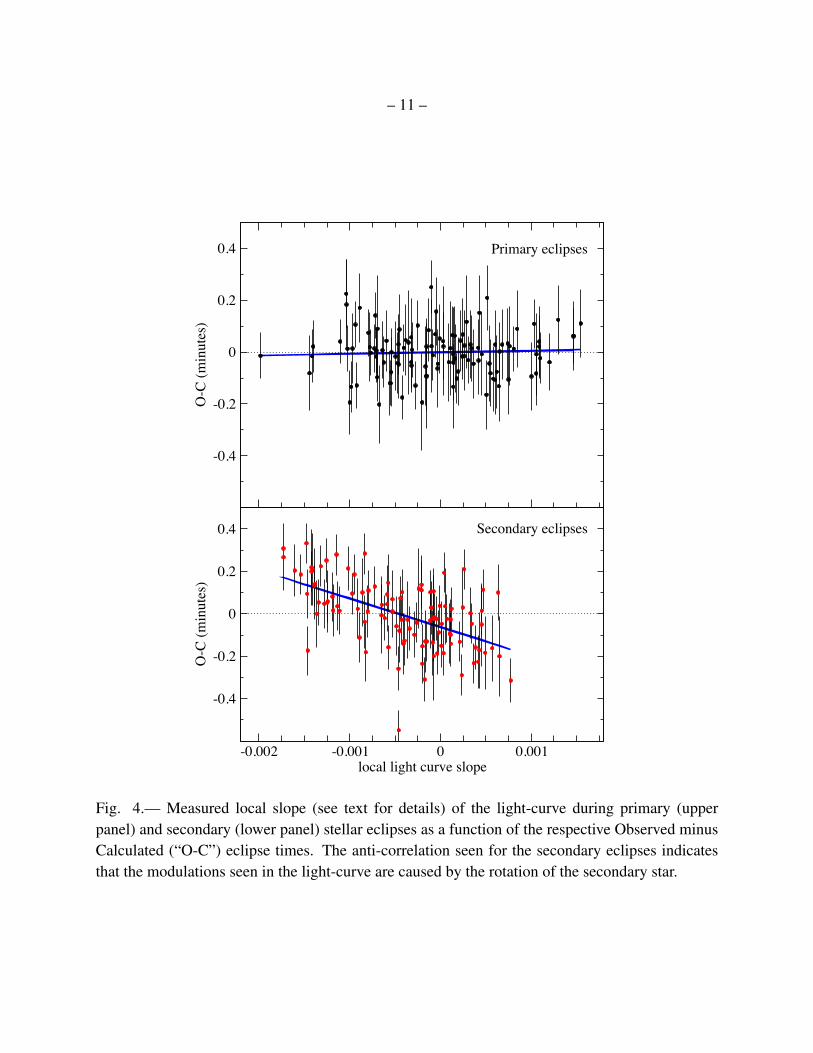
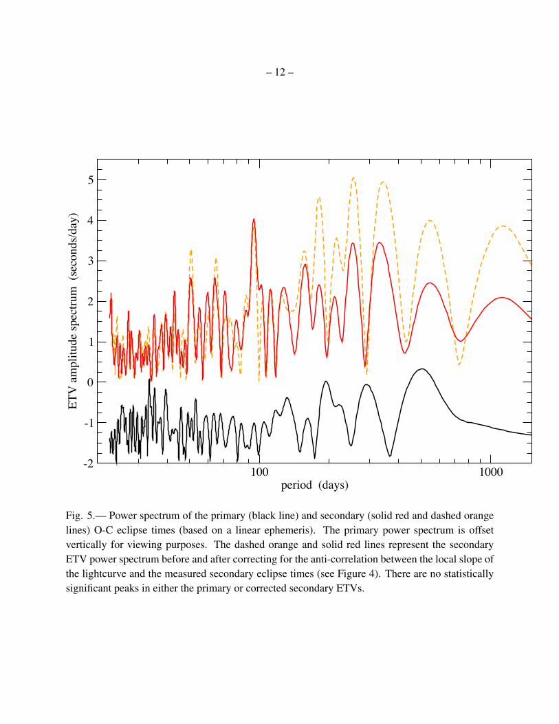
Following the method of Welsh et al. (2015), we also analyzed the effect of star spots on themeasured eclipse times by comparing the local slope of the light-curve outside the stellar eclipsesto the measured ETVs (see also Orosz et al. 2012; Mazeh, Holczer, Shporer 2015; Holczer, etal. 2015). While there is no apparent correlation for the primary eclipse ETVs (Figure 4, left panel),we found a clear, negative correlation for the secondary eclipses (Figure 4, right panel), indicatingthat the observed light-curve modulations are due to the rotationally-modulated signature of starspots moving across the disk of the secondary star. The negative correlation also indicates that thespin and orbital axes of the secondary star are well aligned (Mazeh et al. 2015, Holczer et al. 2015).We have corrected the secondary eclipse times for this anti-correlation. We note that as the lightfrom the secondary is diluted by the primary star, its intrinsic photometric modulations are largerthan the observed 0.1−0.3%, indicating a rather active secondary star. The power spectrum of theO-C ETVs (in terms of measured primary and secondary eclipse times minus linear ephemeris) areshown in Figure 5. There are no statistically significant features in the power spectrum.

The exquisite quality of the Kepler data also allowed for precise measurement of the photo-metric centroid position of the target. Apparent shifts in this position indicate either a contamina-tion from nearby sources (if the centroid shifts away from the target during an eclipse or transit), orthat the source of the studied signal is not the Kepler target itself (if the shift is towards the targetduring an eclipse or transit, see Conroy et al. 2014). As expected, Kepler-1647 exhibits a clearphotocenter shift away from the target and toward the nearby star during the eclipses, indicatingthat the eclipses are indeed coming from the target stars, and that some light contamination from a

2The GR contribution is fixed for the respective masses, period and eccentricity of the binary star

– 10 –

Fig. 3.— Upper panel: Measured “Common Period Observed minus Calculated” (CPOC, or O-C for short) for the primary (black symbols) and secondary (red symbols) stellar eclipses; therespective lines indicate the best-fit photodynamical model. The divergent nature of the CPOCsconstrains the mass of the CBP. Lower panel: CPOC residuals based on the photodynamical model.The respective average error bars are shown in the lower left of the upper panel.

– 11 –

-0.4

-0.2

0

0.2

0.4

O-C

(min

utes

)

Primary eclipses

-0.002 -0.001 0 0.001local light curve slope

-0.4

-0.2

0

0.2

0.4

O-C

(min

utes

)

Secondary eclipses

Fig. 4.— Measured local slope (see text for details) of the light-curve during primary (upperpanel) and secondary (lower panel) stellar eclipses as a function of the respective Observed minusCalculated (“O-C”) eclipse times. The anti-correlation seen for the secondary eclipses indicatesthat the modulations seen in the light-curve are caused by the rotation of the secondary star.

– 12 –

100 1000period (days)

-2

-1

0

1

2

3

4

5

ETV

am

plitu

de sp

ectru

m (

seco

nds/

day)

Fig. 5.— Power spectrum of the primary (black line) and secondary (solid red and dashed orangelines) O-C eclipse times (based on a linear ephemeris). The primary power spectrum is offsetvertically for viewing purposes. The dashed orange and solid red lines represent the secondaryETV power spectrum before and after correcting for the anti-correlation between the local slope ofthe lightcurve and the measured secondary eclipse times (see Figure 4). There are no statisticallysignificant peaks in either the primary or corrected secondary ETVs.

– 13 –

nearby star is present in the Kepler aperture. We discuss this in more details in Section 3.3.

2.2. Stellar Rotation

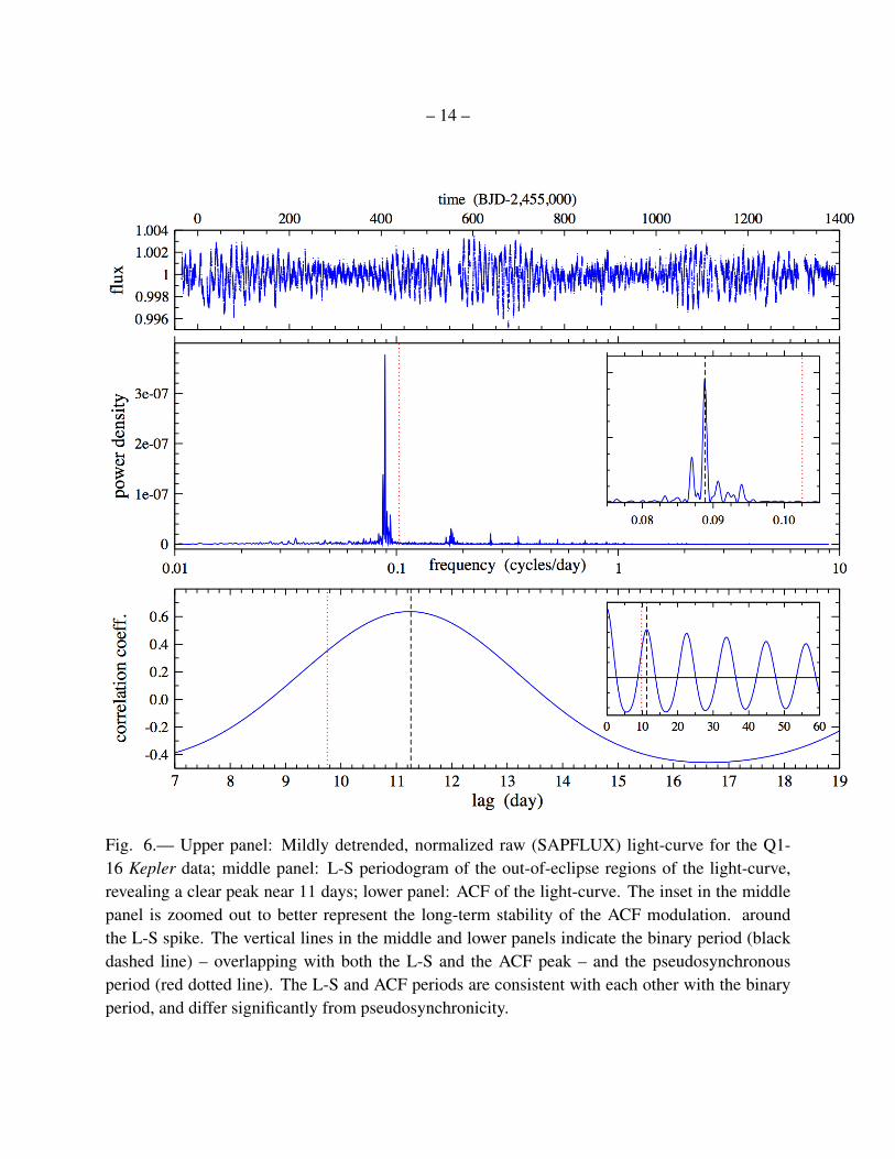
The out-of-eclipse sections of the light-curve are dominated by quasi-periodic flux modu-lations with an amplitude of 0.1− 0.3% (lower panel, Figure 1). To measure the period of thesemodulations we performed both a Lomb-Scargle (L-S) and an autocorrelation function (ACF) anal-ysis of the light-curve. For the latter method, based on measuring the time lags of spot-inducedACF peaks, we followed the prescription of McQuillan et al. (2013, 2014). Both methods showclear periodic modulations (see Figure 1 and Figure 6), with Prot = 11.23±0.01 days – very closeto the orbital period of the binary. We examined the light-curve by eye and confirmed that this isindeed the true period.

To measure the period, we first removed the stellar eclipses from the light curve using a maskthat was 1.5 times the duration of the primary eclipse (0.220 days) and centered on each eclipsetime. After the eclipses were removed, a 7th order polynomial was used to moderately detrendeach Quarter. In Figure 6 we show the mildly detrended SAPFLUX light-curve covering Q1-16Kepler data (upper panel), the power spectrum as a function of the logarithmic frequency (middlepanel) and the ACF of the light-curve (lower panel). Each Quarter shown in the upper panel hada 7th order polynomial fit divided out to normalize the light-curve, and we also clipped out themonthly data-download glitches by hand, and any data with Data Quality Flag >8. The inset inthe lower panel zooms out on to better show the long-term stability of the ACF; the vertical blackdashed lines in the middle and lower panels represent the best fit orbital period of the binary star,and the red dotted lines represent the expected rotation period if the system were in pseudosyn-chronous rotation. The periods as derived from the ACF and from L-S agree exactly.

The near-equality between the orbital and the rotation period raises the question whether thestars could be in pseudosynchronous pseudo-equilibrium. If this is the case, then with Pbin =

11.258818 days and ebin = 0.16, and based on Hut’s formula (Hut 1981, 1982), the expectedpseudosynchronous period is Ppseudo,rot = 9.75 days. Such spin-orbit synchronization should havebeen reached within a Gyr3. Thus the secondary star is not rotating pseudosynchronously. This isclearly illustrated in Figure 6, where the red dotted line in the inset in the lower panel representsthe pseudosynhronous rotation period.

Our measurement of the near-equality between Prot and Pbin indicates that the rotation of bothstars is synchronous with the binary period (due to tidal interaction with the binary orbit). Thus the

3Orbital circularization takes orders of magnitude longer and is not expected.

– 14 –

Fig. 6.— Upper panel: Mildly detrended, normalized raw (SAPFLUX) light-curve for the Q1-16 Kepler data; middle panel: L-S periodogram of the out-of-eclipse regions of the light-curve,revealing a clear peak near 11 days; lower panel: ACF of the light-curve. The inset in the middlepanel is zoomed out to better represent the long-term stability of the ACF modulation. aroundthe L-S spike. The vertical lines in the middle and lower panels indicate the binary period (blackdashed line) – overlapping with both the L-S and the ACF peak – and the pseudosynchronousperiod (red dotted line). The L-S and ACF periods are consistent with each other with the binaryperiod, and differ significantly from pseudosynchronicity.

– 15 –

secondary (G-type) star appears to be tidally spun up since its rotation period is faster than expectedfor its spectral type and age (discussed in more detail in Section 5), and has driven the large stellaractivity, as seen by the large amplitude star spots. The primary star does not appear to be active.The spin-up of the primary (an F-type star) should not be significant since F-stars naturally rotatefaster, and are quieter than G-stars (assuming the same age). As a result, the primary could seemquiet compared to the secondary – but this can change as the primary star evolves. As seen fromFigure 6, the starspot modulation is indeed at the binary orbital period (black dashed line, inset inlower panel).

There is reasonable evidence that stars evolving off the main sequence look quieter than mainsequence stars (at least for a while); stars with shallower convection zones look less variable at agiven rotation rate (Bastien et al. 2014). The convective zone of the primary star is probably toothin for significant spot generation at that rotation period. As we show in Section 5, the secondarystar has mass and effective temperature very similar to the Sun, so it should be generating spots atabout the same rate as the Sun would have done when it was at the age of NGC 6811 – where earlyG stars have rotation periods of 10-12 days (Meibom et al 2011).

Based on the photodynamically-calculated stellar radii RA and RB (Section 5), and on themeasured Prot, if the two stars are indeed synchronized then their rotational velocities shouldbe Vrot,A sin iA = 8.04 km/s and Vrot,B sin iB = 4.35 km/s. If, on the contrary, the two stars arerotating pseudosynchronously, their respective velocities should be Vrot,A sin iA = 9.25 km/s andVrot,B sin iB = 5.00 km/s.

The spectroscopically-measured rotational velocities (Section 3.1) are Vrot,A sin iA = 8.4±0.5km/s and Vrot,B sin iB = 5.1± 1.0 km/s respectively – assuming 5.5 km/s macroturbulence for theprimary star (Doyle et al. 2014), and 3.98 km/s macroturbulence for Solar-type stars (Gray 1984)as appropriate for the secondary. Given the uncertainty on both the measurements and the assumedmacroturbulence, the measured rotational velocities are not inconsistent with synchronization.

Combined with the measured rotation period, and assuming spin-orbit synchronization of thebinary, the measured broadening of the spectral lines constrain the stellar radii:

RB =ProtVrot,B sin iB

2πφ(1)

where φ accounts for differential rotation and is a factor of order unity. Assuming φ = 1, RB =

1.1±0.2 R and RA = 1.85 RB (see Table 2) = 2.08±0.37 R.

– 16 –

3. Spectroscopic and Photometric follow-up observations

To complement the Kepler data, and better characterize the Kepler-1647 system, we obtainedcomprehensive spectroscopic and photometric follow-up observations. Here we describe the radialvelocity measurements we obtained to constrain the spectroscopic orbit of the binary and calculatethe stellar masses, its orbital semi-major axis, eccentricity and argument of periastron. We alsopresent our spectroscopic analysis constraining the effective temperature, metallicity and surfacegravity of the two stars, our direct-imaging observations aimed at estimating flux contaminationdue to unresolved background sources, and our ground-based observations of stellar eclipses toextend the accessible time baseline past the end of the original Kepler mission.

3.1. Spectroscopic follow-up and Radial Velocities

We monitored Kepler-1647 spectroscopically with several instruments in order to measure theradial velocities of the two components of the EB. Observations were collected with the Tilling-hast Reflector Echelle Spectrograph (TRES; Furesz 2008) on the 1.5-m telescope at the Fred L.Whipple Observatory, the Tull Coude Spectrograph (Tull et al. 1995) on the McDonald Observa-tory 2.7-m Harlan J. Smith Telescope, the High Resolution Echelle Spectrometer (HIRES; Vogt etal. 1994) on the 10-m Keck I telescope at the W. M. Keck Observatory, and the Hamilton EchelleSpectrometer (HamSpec; Vogt 1987) on the Lick Observatory 3-m Shane telescope.

A total of 14 observations were obtained with TRES (eight in 2011, five in 2012, and onein 2013). They span the wavelength range from about 390 to 900 nm at a resolving power ofR≈ 44,000. We extracted the spectra following the procedures outlined by Buchhave et al. (2010).Seven observations were gathered with the Tull Coude Spectrograph in 2011, each consisting ofthree exposures of 1200 seconds. This instrument covers the wavelength range 380–1000 nmat a resolving power of R ≈ 60,000. The data were reduced and extracteded with the instru-ment pipeline. Two observations were obtained with HIRES also in 2011, covering the range300-1000 nm at a resolving power of R ≈ 60,000 at 550 nm. We used the C2 decker for skysubtraction, giving a sky-projected area for the slit of 0.′′87× 14.′′0. Th-Ar lamp exposures wereused for wavelength calibration, and the spectra were extracteded with the pipeline used for planetsearch programs at that facility. Finally, two spectra were collected with HamSpec in 2011, with awavelength coverage of 385–955 nm and a resolving power of R≈ 60,000.

All of these spectra are double-lined.4 RVs for both binary components from the TRES spectra

4We note that Kolbl et al. (2015) detected the spectrum of the secondary star as well, and obtained its effectivetemperature (Teff,B ∼ 5900 K) and flux ratio (FB/FA = 0.22) – fully consistent with our analysis.

– 17 –

were derived using the two-dimensional cross-correlation technique TODCOR (Zucker & Mazeh1994), with templates taken from a library of synthetic spectra generated from model atmospheresby R. L. Kurucz (see Nordstrom et al. 1994; Latham et al. 2002). These templates were calculatedby John Laird, based on a line list compiled by Jon Morse. The synthetic spectra cover 30 nmcentered near 519 nm, though we only used the central 10 nm, corresponding to the TRES echelleorder centered on the gravity-sensitive Mg I b triplet. Template parameters (effective temperature,surface gravity, metallicity, and rotational broadening) were selected as described in the next sec-tion.

To measure the RVs from the other three instruments, we used the “broadening function”(BF) technique (e.g., Schwamb et al. 2013), in which the Doppler shift can be obtained fromthe centroid of the peak corresponding to each component in the broadening function, and therotational broadening is measured from the peak’s width. This method requires a high-resolutiontemplate spectrum of a slowly rotating star, for which we used the RV standard star HD 182488(a G8V star with a RV of +21.508 km s−1; see Welsh et al. 2015). All HJDs in the CoordinatedUniversal Time (UTC) frame were converted to BJDs in the Terrestrial Time (TT) frame using thesoftware tools by Eastman et al. (2010). It was also necessary to adjust the RV zero points to matchthat of TRES by +0.66 km s−1 for McDonald, −0.16 km s−1 for Lick, and by +0.28 km s−1 forKeck. We report all radial velocity measurements in Table 1.

3.2. Spectroscopic Parameters

In order to derive the spectroscopic parameters (Teff, logg, [m/H], vsin i) of the components ofthe Kepler-1647 binary, both for obtaining the final radial velocities and also for later use in com-paring the physical properties of the stars with stellar evolution models, we made use of TODCORas a convenient tool to find the best match between our synthetic spectra and the observations.Weak spectra or blended lines can prevent accurate classifications, so we included in this analysisonly the 11 strongest TRES spectra (S/N > 20), and note that all of these spectra have a velocityseparation greater than 30 km s−1 between the two stars.

We performed an analysis similar to the one used to characterize the stars of the CBP-hostingdouble-lined binaries Kepler-34 and Kepler-35 (Welsh et al. 2012), but given slight differences inthe analysis that are required by the characteristics of this system, we provide further details here.We began by cross-correlating the TRES spectra against a (five-dimensional) grid of synthetic com-posite spectra that we described in the previous section. The grid we used for Kepler-1647 containsevery combination of stellar parameters in the ranges Teff,A = [4750,7500], Teff,B = [4250,7250],loggA = [3.0,5.0], loggB = [3.5,5.0], and [m/H]= [−1.0,+0.5], with grid spacings of 250 K in

– 18 –

Teff, and 0.5 dex in logg and [m/H] (12,480 total grid points).5 At each step in the grid, TODCORwas run in order to determine the RVs of the two stars and the light ratio that produces the best-fitset of 11 synthetic composite spectra, and we saved the resulting mean correlation peak heightfrom these 11 correlations. Finally, we interpolated along the grid surface defined by these peakheights to arrive at the best-fit combination of stellar parameters.

This analysis would normally be limited by the degeneracy between spectroscopic parame-ters (i.e., a nearly equally good fit can be obtained by slightly increasing or decreasing Teff, logg,and [m/H] in tandem), but the photodynamical model partially breaks this degeneracy by provid-ing precise, independently determined surface gravities. We interpolated to these values in ouranalysis and were left with a more manageable Teff-[m/H] degeneracy. In principle one could usetemperatures estimated from standard photometry to help constrain the solution and overcome theTeff-[m/H] correlation, but the binary nature of the object (both stars contributing significant light)and uncertainties in the reddening make this difficult in practice. In the absence of such an externalconstraint, we computed a table of Teff,A and Teff,B values as a function of metallicity, and foundthe highest average correlation value for [m/H] = −0.18, leading to temperatures of 6190 and5760 K for the primary and secondary of Kepler-1647, respectively. The average flux ratio fromthis best fit is FB/FA = 0.21 at a mean wavelength of 519 nm. To arrive at the final spectroscopicparameters, we elected to resolve the remaining degeneracy by appealing to stellar evolution mod-els. This procedure is described below in Section 5.1, and results in slightly adjusted values of[m/H] = −0.14± 0.056 and temperatures of 6210 and 5770 K, with estimated uncertainties of100 K.

3.3. Direct imaging follow-up

Due to Kepler’s large pixel size (3.98′′, Koch et al. 2010), it is possible for unresolved sourcesto be present inside the target’s aperture, and to also contaminate its light-curve. A data query fromMAST indicates that the Kepler-1647 suffers a mean contamination of 4± 1% between the fourseasons. To fully account for the effect this contamination has on the inferred sizes of the occultingobjects, we performed an archival search and pursued additional photometric observations.

A nearby star to the south of Kepler-1647 is clearly resolved on UKIRT/WFCAM J-bandimages (Lawrence et al. 2007), with ∆J = 2.2 mag and separation of 2.8′′. Kepler-1647 was also

5We ran a separate TODCOR grid solely to determine the vsin i values, which we left fixed in the larger grid. This isjustified because the magnitude of the covariance between vsin i and the other parameters is small. This simplificationreduces computation time by almost two orders of magnitude.

6Note the difference from the NexSci catalog value of -0.78.

– 19 –

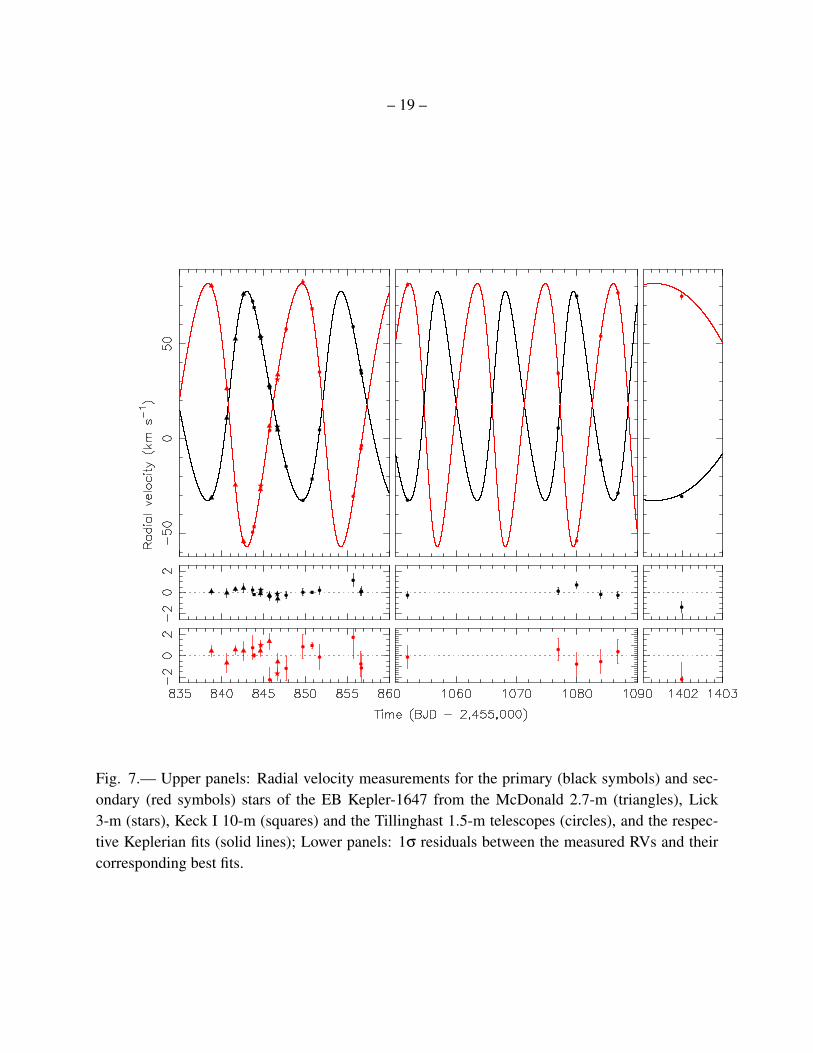
Fig. 7.— Upper panels: Radial velocity measurements for the primary (black symbols) and sec-ondary (red symbols) stars of the EB Kepler-1647 from the McDonald 2.7-m (triangles), Lick3-m (stars), Keck I 10-m (squares) and the Tillinghast 1.5-m telescopes (circles), and the respec-tive Keplerian fits (solid lines); Lower panels: 1σ residuals between the measured RVs and theircorresponding best fits.

– 20 –

observed in g-, r-, i-bands, and Hα from the INT survey (Greiss et al. 2012). The respectivemagnitude differences between the EB and the companion are ∆g = 3.19,∆r = 2.73,∆Hα = 2.61,and ∆i = 2.52 mag with formal uncertainties below 1%. Based on Equations 2 through 5 fromBrown et al. (2011) to convert from Sloan to Kp, these correspond to magnitude and flux differencesbetween the EB and the companion star of ∆Kp = 2.73 and ∆F = 8%. In addition, adaptive-opticsobservations by Dressing et al. (2014) with MMT/ARIES detected the companion at a separationof 2.78′′ from the target, with ∆Ks = 1.84 mag, estimated ∆Kp = 2.2 mag, and reported a positionangle for the companion of 131.4 (East of North).

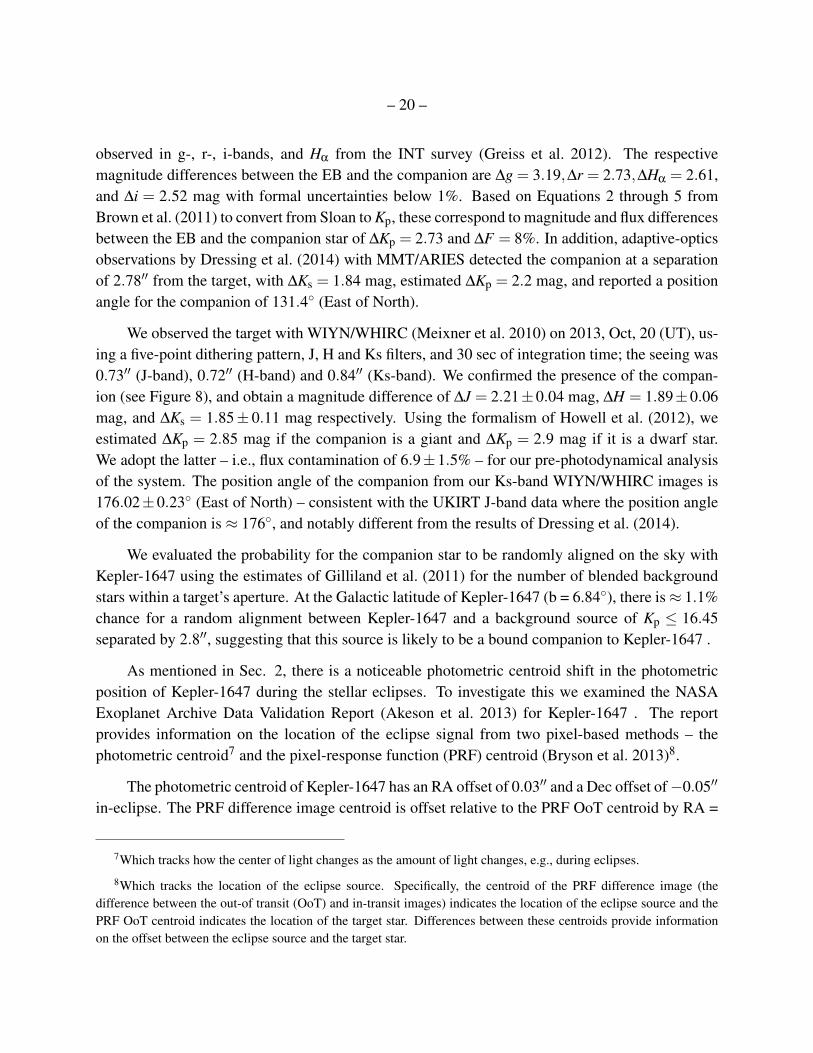
We observed the target with WIYN/WHIRC (Meixner et al. 2010) on 2013, Oct, 20 (UT), us-ing a five-point dithering pattern, J, H and Ks filters, and 30 sec of integration time; the seeing was0.73′′ (J-band), 0.72′′ (H-band) and 0.84′′ (Ks-band). We confirmed the presence of the compan-ion (see Figure 8), and obtain a magnitude difference of ∆J = 2.21±0.04 mag, ∆H = 1.89±0.06mag, and ∆Ks = 1.85± 0.11 mag respectively. Using the formalism of Howell et al. (2012), weestimated ∆Kp = 2.85 mag if the companion is a giant and ∆Kp = 2.9 mag if it is a dwarf star.We adopt the latter – i.e., flux contamination of 6.9±1.5% – for our pre-photodynamical analysisof the system. The position angle of the companion from our Ks-band WIYN/WHIRC images is176.02±0.23 (East of North) – consistent with the UKIRT J-band data where the position angleof the companion is ≈ 176, and notably different from the results of Dressing et al. (2014).

We evaluated the probability for the companion star to be randomly aligned on the sky withKepler-1647 using the estimates of Gilliland et al. (2011) for the number of blended backgroundstars within a target’s aperture. At the Galactic latitude of Kepler-1647 (b = 6.84), there is≈ 1.1%chance for a random alignment between Kepler-1647 and a background source of Kp ≤ 16.45separated by 2.8′′, suggesting that this source is likely to be a bound companion to Kepler-1647 .

As mentioned in Sec. 2, there is a noticeable photometric centroid shift in the photometricposition of Kepler-1647 during the stellar eclipses. To investigate this we examined the NASAExoplanet Archive Data Validation Report (Akeson et al. 2013) for Kepler-1647 . The reportprovides information on the location of the eclipse signal from two pixel-based methods – thephotometric centroid7 and the pixel-response function (PRF) centroid (Bryson et al. 2013)8.

The photometric centroid of Kepler-1647 has an RA offset of 0.03′′ and a Dec offset of−0.05′′

in-eclipse. The PRF difference image centroid is offset relative to the PRF OoT centroid by RA =

7Which tracks how the center of light changes as the amount of light changes, e.g., during eclipses.

8Which tracks the location of the eclipse source. Specifically, the centroid of the PRF difference image (thedifference between the out-of transit (OoT) and in-transit images) indicates the location of the eclipse source and thePRF OoT centroid indicates the location of the target star. Differences between these centroids provide informationon the offset between the eclipse source and the target star.

– 21 –

Fig. 8.— A J-band WIYN/WHIRC image of Kepler-1647 showing the nearby star to the south ofthe EB. The size of the box is 30′′ by 30′′. The two stars are separated by 2.89±0.14′′.

– 22 –

−0.012′′ and Dec = 0.136′′ respectively (the offsets relative to the KIC position are RA =−0.019′′

and Dec = 0.01′′). Both methods indicate that the measured center of light shifts away fromKepler-1647 during the stellar eclipses, fully consistent with the photometric contamination fromthe companion star to the SE of the EB.

3.4. Time-series photometric follow-up

In order to confirm the model derived from the Kepler data and to place additional constraintson the model over a longer time baseline, we undertook additional time-series observations ofKepler-1647 using the KELT follow-up network, which consists of small and mid-size telescopesused for confirming transiting planets for the KELT survey (Pepper, et al. 2007; Siverd, et al. 2012).Based on predictions of primary eclipse times for Kepler-1647, we obtained two observations ofpartial eclipses after the end of the Kepler primary mission. The long durations of the primaryeclipse (> 9 hours) make it nearly impossible to completely observe from any one site, but partialeclipses can nevertheless help constrain the eclipse time.

We observed a primary eclipse simultaneously in V and i at Swarthmore College’s Peter vande Kamp Observatory on UT2013-08-17. The observatory uses a 0.6 m RCOS Telescope withan Apogee U16M 4K× 4K CCD, giving a 26′× 26′ field of view. Using 2× 2 binning, it has0.76′′/pixel. These observations covered the second half of the eclipse, extending about 2.5 hoursafter egress.

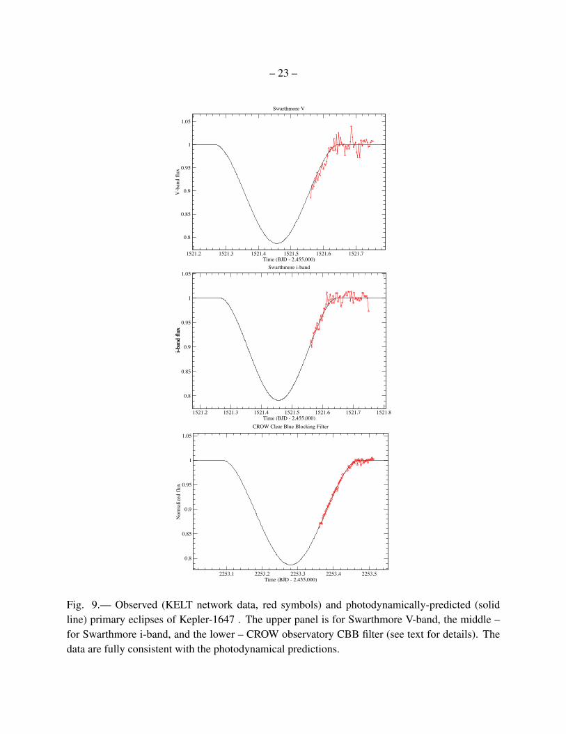
We observed a primary eclipse of the system at Canela’s Robotic Observatory (CROW) inPortugal. Observations were made using a 0.3 m LX200 telescope with a SBIG ST-8XME CCD.The FOV is 28′× 19′ and 1.11′′/pixel. Observations were taken on UT2015-08-18 using a clear,blue-blocking (CBB) filter. These observations covered the second half of the eclipse, extendingabout 1 hour after egress. The observed eclipses from KELT, shown in Figure 9 match well withthe forward photodynamical models (Sec. 4.2).

To complement the Kepler data, we used the 1-m Mount Laguna Observatory telescope to ob-serve Kepler-1647 at the predicted times for planetary transits in the summer of 2015 (see Table 7).Suboptimal observing conditions thwarted our efforts and, unfortunately, we were unable to detectthe transits. The obtained images, however, confirmed the presence and orientation of the nearbystar to the south of Kepler-1647.

– 23 –

1521.2 1521.3 1521.4 1521.5 1521.6 1521.7Time (BJD - 2,455,000)

0.8

0.85

0.9

0.95

1

1.05

V-b

and

flux

KOI 2939Swarthmore V

1521.2 1521.3 1521.4 1521.5 1521.6 1521.7 1521.8Time (BJD - 2,455,000)

0.8

0.85

0.9

0.95

1

1.05

i mag

nitu

de

KOI 2939Swarthmore i-band

i-ban

d flu

xi-b

and

flux

2253.1 2253.2 2253.3 2253.4 2253.5Time (BJD - 2,455,000)

0.8

0.85

0.9

0.95

1

1.05

Nor

mal

ized

flux

KOI 2939CROW Clear Blue Blocking Filter

Fig. 9.— Observed (KELT network data, red symbols) and photodynamically-predicted (solidline) primary eclipses of Kepler-1647 . The upper panel is for Swarthmore V-band, the middle –for Swarthmore i-band, and the lower – CROW observatory CBB filter (see text for details). Thedata are fully consistent with the photodynamical predictions.

– 24 –

4. Unraveling the system

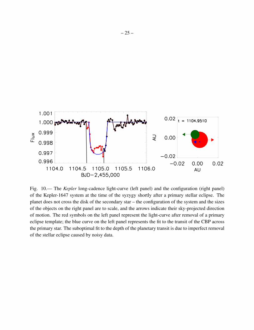
Kepler-1647b produced three transits: two across the secondary star at tB,1 = −3.0018 andtB,2 = 1109.2612 (BJD-2,455,000), corresponding to EB phase of 0.60 and 0.39 respectively, andone heavily blended transit across the primary star at time tA,1 – a syzygy (the secondary starand the planet simultaneously cross the line of sight between Kepler and the disk of the primarystar) during a primary stellar eclipse at tprim = 1104.8797. The latter transit is not immediatelyobvious and requires careful inspection of the light-curve. We measured transit durations across thesecondary of tdur,B,1 = 0.137 days and tdur,B,2 = 0.279 days. The light-curve and the configurationof the system at the time of the syzygy are shown in Figure 10.

To extract the transit center time and duration across the primary star, tA and tdur,A, we sub-tracted a primary eclipse template from the data, then measured the mid-transit time and durationfrom the residual light-curve – now containing only the planetary transit – to be tA = 1104.9510(BJD-2,455,000), corresponding to EB phase 0.006, and tdur,A = 0.411 days. From the transitdepths, and accounting from dilution, we estimated kp,prim = Rp/RA = 0.06 and kp,sec = Rp/RB =

0.11. We outline the parameters of the planetary transits in Table 7. As expected from a CBP, thetwo transits across the secondary star vary in both depth and duration, depending on the phase ofthe EB at the respective transit times. This unique observational signature rules out common falsepositives (such as a background EB) and confirms the nature of the planet. In the following sectionwe describe how we used the center times and durations of these three CBP transits to analyticallydescribe the planet’s orbit.

4.1. Analytic treatment

As discussed in Schneider & Chevreton (1990) and Kostov et al. (2013), the detection ofCBP transits across one or both stars during the same inferior conjunction (e.g., Kepler-34, -35and now Kepler-1647 ) can strongly constrain the orbital configuration of the planet when the hostsystem is an SB2 eclipsing binary. Such scenario, dubbed “double-lined, double-dipped” (Kostovet al. 2013), is optimal in terms of constraining the a priori unknown orbit of the CBP.

4.1.1. CBP transit times

Using the RV measurements of the EB (Table 1) to obtain the x- and y-coordinates of thetwo stars at the times of the CBP transits, and combining these with the measured time intervalbetween two consecutive CBP transits, we can estimate the orbital period and semi-major axis of

– 25 –

Fig. 10.— The Kepler long-cadence light-curve (left panel) and the configuration (right panel)of the Kepler-1647 system at the time of the syzygy shortly after a primary stellar eclipse. Theplanet does not cross the disk of the secondary star – the configuration of the system and the sizesof the objects on the right panel are to scale, and the arrows indicate their sky-projected directionof motion. The red symbols on the left panel represent the light-curve after removal of a primaryeclipse template; the blue curve on the left panel represents the fit to the transit of the CBP acrossthe primary star. The suboptimal fit to the depth of the planetary transit is due to imperfect removalof the stellar eclipse caused by noisy data.

– 26 –

the CBP – independent of and complementary to the photometric-dynamical model presented inthe next Section. Specifically, the CBP travels a known distance ∆x for a known time ∆t betweentwo consecutive transits across either star (but during the same inferior conjunction), and its x-component velocity is9:

Vx,p =∆x∆t

∆x = |xi− x j|∆t = |ti− t j|

(2)

where xi, j is the x-coordinate of the star being transited by the planet at the observed mid-transittime of ti, j. As described above, the CBP transited across the primary and secondary star during thesame inferior conjunction, namely at ti = tA = 1104.9510±0.0041, and at t j = tB,2 = 1109.2612±0.0036 (BJD-2,455,000). Thus ∆t = 4.3102±0.0055 days.

The barycentric x-coordinates of the primary and secondary stars are (Hilditch, 2001)10:

xA,B(tA,B) = rA,B(tA,B)cos[θA,B(tA,B)+ωbin] (3)

where rA,B(tA,B) is the radius-vector of each star at the times of the CBP transits tA and tB,2:

rA,B(tA,B) = aA,B(1− e2bin)[1+ ebin cos(θA,B(tA,B))]

−1 (4)

where θA,B(tA,B) are the true anomalies of the primary and secondary stars at tA and tB, ebin =

0.159±0.003 and ωbin = 300.85±0.91 are the binary eccentricity and argument of periastron asderived from the spectroscopic measurements (see Table 1). Using the measured semi-amplitudesof the RV curves for the two host stars (KA = 55.73±0.21 km/sec and KB = 69.13±0.5 km/sec,see Table 1), and the binary period Pbin = 11.2588 days, the semi major axes of the two stars areaA = 0.0569± 0.0002 AU and aB = 0.0707± 0.0005 AU respectively (Equation 2.51, Hilditch(2001)).

To find θA,B(tA,B) we solved Kepler’s equation for the two eccentric anomalies11, EA,B−ebin sin(EA,B) = 2π(tA,B− t0)/Pbin, where t0 =−47.869±0.003 (BJD−2,455,000) is the time of

9The observer is at +z, and the sky is in the xy-plane.

10The longitude of ascending node of the binary star, Ωbin, is undefined and set to zero throughout this paper.

11Taking into account that ω for the primary star is ωbin−π

– 27 –

periastron passage for the EB, and obtain θA(tA) = 2.64± 0.03 rad, θB(tB,2) = 4.55± 0.03 rad.The radius vector of each star is then rA(tA) = 0.065±0.003 AU and rB(tB) = 0.071±0.004 AU,and from Equation 3, xA(tA) = 0.0020± 0.0008 AU and xB(tB) = −0.0658± 0.0009 AU. Thus∆x = 0.0681±0.0012 AU and, finally, Vx,p = 0.0158±0.0006 AU/day (see Equation 2).

Next, we used Vx,p to estimate the period and semi-major axes of the CBP as follows. Thex-component of the planet’s velocity, assuming that cos(Ωp) = 1 and cos(ip) = 0 where Ωp and ipare the planet’s longitude of ascending node and inclination respectively in the reference frame ofthe sky)12 is:

Vx,p =−(

2πGMbin

Pp

)1/3 [ep sinωp + sin(θp +ωp)]√(1− e2

p)(5)

where Mbin = 2.19±0.02 M is the mass of the binary star (calculated from the measured radialvelocities of its two component stars – Equation 2.52, Hilditch 2001), and Pp,ep,ωp and θp arethe orbital period, eccentricity, argument of periastron and the true anomaly of the planet. Whenthe planet is near inferior conjunction, like during the transits at tA and tB,2, we can approximatesin(θp +ωp) = 1. Simple algebra shows that:

Pp = 1080(1+ ep sinωp)

3

(1− e2p)

3/2 [days] (6)

Thus if the orbit of Kepler-1647b is circular, its orbital period is Pp ≈ 1100 days and its semi-majoraxis is ap ≈ 2.8 AU. In this case we can firmly rule out a CBP period of 550 days.

Even if the planet has a non-zero eccentricity, Equation 6 still allowed us to constrain theorbit it needs to produce the two transits observed at tA and tB,2. In other words, if Pp is indeednot ∼ 1100 days but half of that (assuming that a missed transit fell into a data gap), then fromEquation 6:

2 (1+ ep sinωp)3 = (1− e2

p)3/2 ≤ 1 (7)

which implies ep ≥ 0.21. Thus Equation 7 indicates that unless the eccentricity of CBP Kepler-1647b is greater than 0.21, its orbital period cannot be half of 1100 days.

12Both consistent with the planet transiting near inferior conjunction.

– 28 –

We note that our Equation 7 differs from Equation 8 in Schneider & Chevreton (1990) by afactor of 4π3. As the two equations describe the same phenomenon (for a circular orbit for theplanet), we suspect there is a missing factor of 2π in the sine and cosine parts of their equations 6aand 6b, which propagated through.

4.1.2. CBP transit durations

As shown by Kostov et al. (2013, 2014) for the cases of Kepler-47b, Kepler-64b and Kepler-413b, and discussed by Schneider & Chevreton (1990), the measured transit durations of CBPscan constrain the a priori unknown mass of their host binary stars13 when the orbital period of theplanets can be estimated from the data. The case of Kepler-1647 is the opposite – the mass ofthe EB is known (from spectroscopic observations) while the orbital period of the CBP cannot bepinned down prior to a full photodynamical solution of the system. However, we can still estimatethe orbital period of Kepler-1647b using its transit durations:

tdur, n =2 Rc, n

Vx,p +Vx,star,n(8)

where Rc,n = Rstar,n√

(1+ kp)2−b2n is the transit chord (where kp,prim = 0.06, kp,sec = 0.11, and bn

the impact parameter) for the n− th CBP transit, Vx,star,n and Vx,p are the x-component velocities ofthe star and of the CBP respectively. Using Equation 5, we can rewrite Equation 8 in terms of Pp

(the orbital period of the planet) near inferior conjunction (sin(θp +ωp) = 1) as:

Pp(tdur,n) = 2πGMbin(1+ ep sinωp)3(

2Rc,n

tdur,n−Vx,star,n

)−3

(1− e2p)−3/2

(9)

where the stellar velocities Vx,star,n can be calculated from the observables (see Equation 3, Kos-tov et al. 2013): Vx,A = 2.75× 10−2 AU/day; Vx,B,1 = 4.2× 10−2 AU/day; and Vx,B,2 = 2×10−2 AU/day. Using the measured values for tdur,A, tdur,B,1, tdur,B,2 (listed in Table 7), and re-quiring bn ≥ 0, for a circular orbit of the CBP we obtained:

13Provided they are single-lined spectroscopic binaries.

– 29 –

Pp(tdur, A) [days]≥ 4076×(

2.4 (RA

R)−2.75

)−3

Pp(tdur, B, 1) [days]≥ 4076×(

4.1 (RA

R)−4.2

)−3

Pp(tdur, B, 2) [days]≥ 4076×(

2 (RA

R)−2

)−3

(10)

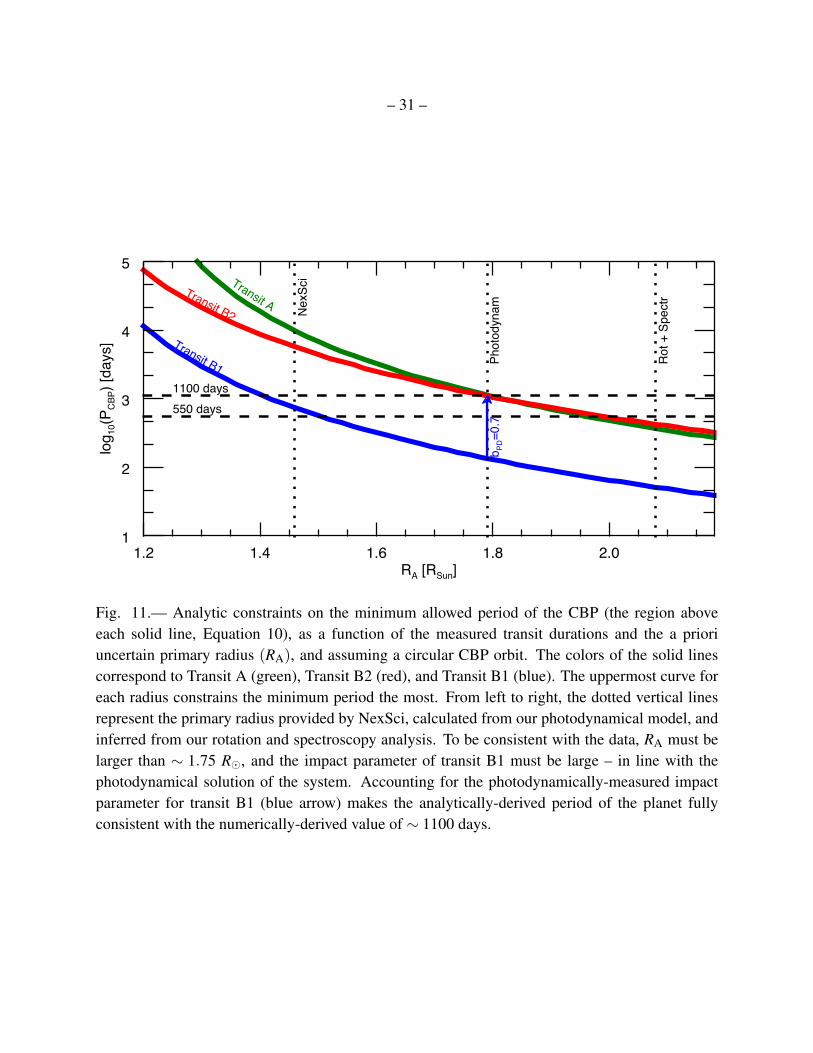
We show these inequalities, defining the allowed region for the period of the CBP as a functionof the (a priori uncertain) primary radius, in Figure 11. The allowed regions for the CBP periodare above each of the solid lines (green for Transit A, Red for Transit B2, and blue for TransitB1), where the uppermost line provides the strongest lower limit for the CBP period at the specificRA. The dotted vertical lines denote, from left to right, the radius provided by NexSci (RA,NexSci =

1.46 R), calculated from our photodynamical model (RA,PD = 1.79 R, Sec 4.2), and inferredfrom the rotation period (RA,rot = 2.08 R). As seen from the figure, RA,NexSci is too small as thecorresponding minimum CBP periods are too long – if this was indeed the primary stellar radiusthen the measured duration of transit A (the strongest constraint at that radius) would correspondto PCBP∼ 104 days (for a circular orbit). The rotationally-inferred radius is consistent with a planeton either a 550-day orbit or a 1100-day orbit but given its large uncertainty (see Section 2.2) theconstraint it provides on the planet period is rather poor.

Thus while the measured transit durations cannot strictly break the degeneracy between a550-day and an 1100-day CBP period prior to a full numerical treatment, they provide usefulconstraints. Specifically, without any prior knowledge of the transit impact parameters, and onlyassuming a circular orbit, Equation 9 indicates that a) the impact parameter of transit B1 must belarge (in order to bring the blue curve close to the other two); and b) RA must be greater than∼ 1.75 R (where the green and red lines intersect) so that the three inequalities in Equation 10are consistent with the data.

We note that Pp in Equation 9 is highly dependent on the impact parameter of the particularCBP transit (which is unknown prior to a full photodynamical solution). Thus a large value for bB,1

will bring the transit B1 curve (blue) closer to the other two. Indeed, our photodynamical modelindicates that bB,1 ≈ 0.7, corresponding to Pp(tdur, B, 1) = 1105 days from Equation 9 (also bluearrow in Figure 11) – bringing the blue curve in line with the other two and validating our analytictreatment of the transit durations. The other two impact parameters, bA,1 and bB,2, are both ≈ 0.2according to the photodynamical model, and do not significantly affect Equation 9 since their con-tribution is small (i.e., b2

A ≈ b2B,2 ≈ 0.04). For the photodynamically-calculated RA,PD = 1.79 R,

the respective analytic CBP periods are Pp(tdur, A)= 1121 days and Pp(tdur, B, 2)= 1093 days. Thus

– 30 –

the analytic analysis presented here is fully consistent with the comprehensive numerical solutionof the system – which we present in the next section.

4.2. Photometric-dynamical solution

CBPs reside in dynamically-rich, multi-parameter space where a strictly Keplerian solution isnot adequate. A comprehensive description of these systems requires a full photometric-dynamicaltreatment based on the available and follow-up data, on N-body simulations, and on the appropriatelight-curve model. We describe this treatment below.

4.2.1. Eclipsing light-curve (ELC)

To obtain a complete solution of the Kepler-1647 system we used the ELC code (Orosz &Hauschildt 2000) with recent “photodynamical” modifications (e.g., Welsh et al. 2015). The codefully accounts for the gravitational interactions between all bodies. Following Mardling & Lin(2002), the gravitational force equations have been modified to account for precession due to Gen-eral Relativistic (GR) effects and due to tides.

Given initial conditions (e.g., masses, positions, and velocities for each body), the code uti-lizes a 12th order symplectic Gaussian Runge-Kutta integrator (Hairer & Hairer 2003) to calculatethe 3-dimensional positions and velocities of the two stars and the planet as a function of time.These are combined with the light-curve model of Mandel & Agol (2002), and the quadratic lawlimb-darkening coefficients, using the “triangular” sampling of Kipping (2013), to calculate modellight and radial velocity curves which are directly compared to the Kepler data (both long- and,where available, short-cadence), the measured stellar radial velocities, and the ground-based light-curves.

The ELC code uses the following as adjustable parameters. The three masses and three sizesof the occulting objects, the Keplerian orbital elements (in terms of Jacobian coordinates) for theEB and the CBP (ebin,ep, ibin, ip,ωbin,ωp,Pbin,Pp, and times of conjunction Tc,bin, Tc,p)14, the CBPlongitude of ascending node Ωp (Ωbin is undefined, and set to zero throughout), the ratio betweenthe stellar temperatures, the quadratic limb-darkening coefficients of each star in the Kepler band-pass and primary limb darkening coefficients for the three bandpasses used for the ground-basedobservations, and the seasonal contamination levels of the Kepler data. The GR modifications to

14The time of conjunction is defined as the conjunction with the barycenter of the system. For the EB, this is closeto a primary eclipse while the CBP does not necessarily transit at conjunction.

– 31 –

Nex

Sci

Phot

odyn

am

Rot

+ S

pect

r

1100 days550 days

b PD=0

.7

1.2 1.4 1.6 1.8 2.0RA [RSun]

1

2

3

4

5

log 1

0(PC

BP) [

days

]

Transit ATransit B2

Transit B1

Fig. 11.— Analytic constraints on the minimum allowed period of the CBP (the region aboveeach solid line, Equation 10), as a function of the measured transit durations and the a prioriuncertain primary radius (RA), and assuming a circular CBP orbit. The colors of the solid linescorrespond to Transit A (green), Transit B2 (red), and Transit B1 (blue). The uppermost curve foreach radius constrains the minimum period the most. From left to right, the dotted vertical linesrepresent the primary radius provided by NexSci, calculated from our photodynamical model, andinferred from our rotation and spectroscopy analysis. To be consistent with the data, RA must belarger than ∼ 1.75 R, and the impact parameter of transit B1 must be large – in line with thephotodynamical solution of the system. Accounting for the photodynamically-measured impactparameter for transit B1 (blue arrow) makes the analytically-derived period of the planet fullyconsistent with the numerically-derived value of ∼ 1100 days.

– 32 –

the force equations require no additional parameters, and the modifications to account for apsidalmotion require the so-called k2 constant and the ratio of the rotational frequency of the star to itspseudosynchronous value for each star. For fitting purposes, we used parameter composites orratios (e.g., ecosω, esinω, MA/MB, RA/RB) as these are generally better constrained by the data.We note that the parameters quoted here are the instantaneous“osculating” values. The coordinatesystem is Jacobian, so the orbit of the planet is referred to the center-of-mass of the binary star.These values are valid for the reference epoch only since the orbits of the EB and the CBP evolvewith time, and must be used in the context of a dynamical model to reproduce our results.

As noted earlier, star spot activity is evident in the Kepler light-curve. After some initial fits,it was found that some of the eclipse profiles were contaminated by star spot activity. We carefullyexamined the residuals of the fit and selected five primary and five secondary eclipses that have“clean” residuals (these are shown in Figure 2). We fit these clean profiles, the times of eclipsefor the remaining eclipse events (corrected for star spot contamination), the three ground-basedobservations, and the two radial velocity curves. We used the observed rotational velocities ofeach star and the spectroscopically determined flux ratio between the two stars (see Tables 1 and2) as additional constraints. The model was optimized using a Differential Evolution Monte CarloMarkov Chain (DE-MCMC, ter Braak 2006). A total of 161 chains were used, and 31,600 gener-ations were computed. We skipped the first 10,000 generations for the purposes of computing theposterior distributions. We adopted the parameters from the best-fitting model, and use posteriordistributions to get the parameter uncertainties.

Throughout the text we quote the best-fit parameters. These do not have error bars and, asnoted above, should be interpreted strictly as the parameters reproducing the light-curve. Foruncertainties the reader should refer to the mode and the mean values calculated from the posteriordistributions.

4.2.2. Consistency check

We confirmed the ELC solution with the photodynam code (Carter et al. 2011, previously usedfor a number of CBPs, e.g., Doyle et al. 2011, Welsh et al. 2012, Schwamb et al. 2013, Kostovet al. 2014). We note, however, that the photodynam code does not include tidal apsidal motion– which must be taken into account for Kepler-1647 as discussed above. Thus while the solutionof the photodynam code provides adequate representation of the light-curve of Kepler-1647 (thedifferences are indistinguishable by eye), it is not the best-fit model in terms of chi-square statistics.

– 33 –

We outline the input for the photodynam code15 required to reproduce the light-curve of Kepler-1647 in Table 6.

We also carried out an analysis using an independent photodynamical code (developed by co-author D.R.S.) that is based on the Nested Sampling concept. This code includes both GR and tidaldistortion. Nested Sampling was introduced by Skilling (2004) to compute the Bayesian Evidence(marginal likelihood or the normalizing factor in Bayes’ Theorem). As a byproduct, a representa-tive sample of the posterior distribution is also obtained. This sample may then be used to estimatethe statistical properties of parameters and of derived quantities of the posterior. MultiNest wasan implementation by Feroz et al. (2008) of Nested Sampling incorporating several improvements.Our version of MultiNest is based on the Feroz code and is a parallel implementation. The Multi-Nest solution confirmed the ELC solution.

5. Results and Discussion

The study of extrasolar planets is first and foremost the study of their parent stars, and tran-siting CBPs, in particular, are a prime example. As we discuss in this section16, their peculiar ob-servational signatures, combined with Kepler’s unmatched precision, help us to not only deciphertheir host systems by a comprehensive photodynamical analysis, but also constrain the fundamen-tal properties of their host stars to great precision. In essence, transiting CBPs allow us to extendthe “royal road” of EBs (Russell 1948) to the realm of exoplanets.

5.1. The Kepler-1647 system

Our best-fit ELC photodynamical solution for Kepler-1647 and the orbital configuration of thesystem are shown in Figure 12 and 13, respectively. The correlations between the major parame-ters are shown in Figure 14. The ELC model parameters are listed in Tables 3 (fitting parameters),4 (derived Keplerian elements) and 5 (derived Cartesian). Table 3 lists the mode and mean ofeach parameter as well as their respective uncertainties as derived from the MCMC posterior dis-tributions; the upper and lower bounds represent the 68% range. The sub-percent precision on thestellar masses and sizes (see the respective values in Table 4) demonstrate the power of photody-namical analysis of transiting CB systems. The parameters presented in Tables 4 and 5 representthe osculating, best-fit model to the Kepler light-curve, and are only valid for the reference epoch

15In terms of osculating parameters.

16And also shown by the previous Kepler CBPs.

– 34 –

(BJD - 2,455,000). These are the parameters that should be used when reproducing the data. Themid-transit times, depths and durations of the observed and modeled planetary transits are listed inTable 7.

The central binary Kepler-1647 is host to two stars with masses of MA = 1.2207±0.0112 M,and MB = 0.9678± 0.0039 M, and radii of RA = 1.7903± 0.0055 R, and RB = 0.9663±0.0057 R, respectively (Table 4). The temperature ratio of the two stars is TB/TA = 0.9365±0.0033 and their flux ratio is FB/FA = 0.21± 0.02 in the Kepler band-pass. The two stars ofthe binary revolve around each other every 11.25882 days in an orbit with a semi-major axisof abin = 0.1276± 0.0002 AU, eccentricity of ebin = 0.1602± 0.0004, and inclination of ibin =

87.9164±0.0145 (see also Table 4 for the respective mean and mode values).

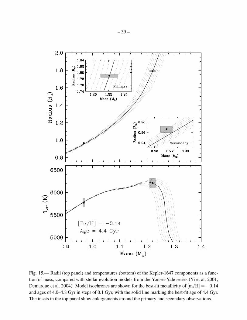
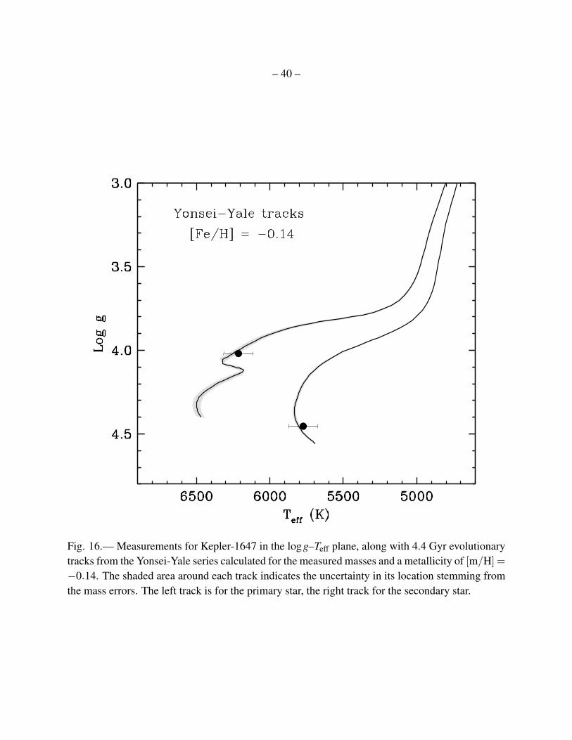
The accurate masses and radii of the Kepler-1647 stars, along with our constraints on thetemperatures and metallicity of this system enable a useful comparison with stellar evolution mod-els. As described in Section 3.2, a degeneracy remains in our determination of [m/H] and Teff,which we resolved here by noting that 1) current models are typically found to match the observedproperties of main-sequence F stars fairly well (see, e.g., Torres et al. 2010), and 2) making theworking assumption that the same should be true for the primary of Kepler-1647, of spectral typeapproximately F8 star. We computed model isochrones from the Yonsei-Yale series (Yi et al. 2001;Demarque et al. 2004) for a range of metallicities. In order to properly compare results from theoryand observation, at each value of metallicity, we also adjusted the spectroscopic temperatures ofboth stars by interpolation in the table of Teff,A and Teff,B versus [m/H] mentioned in Section 3.2.This process led to an excellent fit to the primary star properties (mass, radius, temperature) fora metallicity of [m/H] = −0.14± 0.05 and an age of 4.4± 0.25 Gyr. This fit is illustrated in themass-radius and mass-temperature diagrams of Figure 15. We found that the temperature of thesecondary is also well fit by the same model isochrone that matches the primary. The radius of thesecondary, however, is only marginally matched by the same model, and appears nominally largerthan predicted at the measured mass. Evolutionary tracks for the measured masses and the samebest-fit metallicity are shown in Figure 16.

One possible cause for the slight tension between the observations and the models for thesecondary in the mass-radius diagram is a bias in either the measured masses or the radii. Whilethe individual masses may indeed be subject to systematic uncertainty, the mass ratio should bemore accurate, and a horizontal shift in the upper panels of Figure 15 can only improve the agree-ment with the secondary at the expense of the primary. Similarly, the sum of the radii is tightlyconstrained by the photodynamical fit, and the good agreement between the spectroscopic andphotometric estimates of the flux ratio (see Table 2) is an indication that the radius ratio is alsoaccurate. The flux ratio is a very sensitive indicator because it is proportional to the square of theradius ratio.

– 35 –

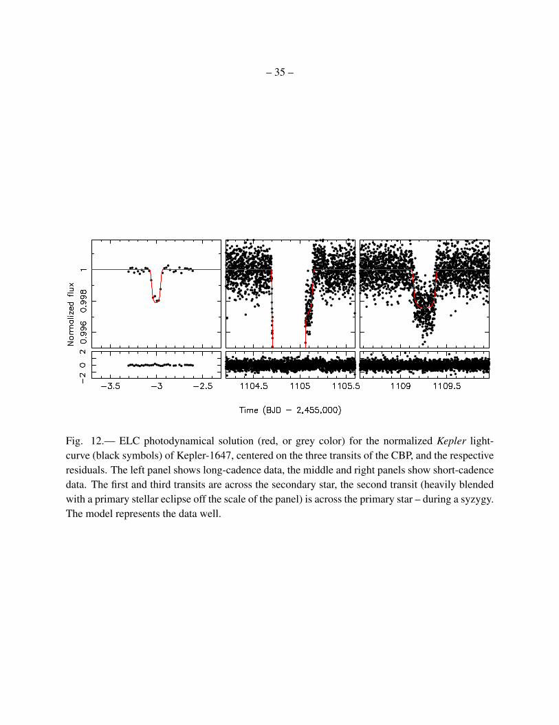
Fig. 12.— ELC photodynamical solution (red, or grey color) for the normalized Kepler light-curve (black symbols) of Kepler-1647, centered on the three transits of the CBP, and the respectiveresiduals. The left panel shows long-cadence data, the middle and right panels show short-cadencedata. The first and third transits are across the secondary star, the second transit (heavily blendedwith a primary stellar eclipse off the scale of the panel) is across the primary star – during a syzygy.The model represents the data well.

– 36 –

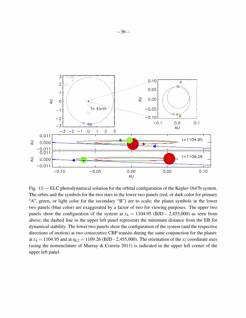
Fig. 13.— ELC photodynamical solution for the orbital configuration of the Kepler-1647b system.The orbits and the symbols for the two stars in the lower two panels (red, or dark color for primary“A”, green, or light color for the secondary “B”) are to scale; the planet symbols in the lowertwo panels (blue color) are exaggerated by a factor of two for viewing purposes. The upper twopanels show the configuration of the system at tA = 1104.95 (BJD - 2,455,000) as seen fromabove; the dashed line in the upper left panel represents the minimum distance from the EB fordynamical stability. The lower two panels show the configuration of the system (and the respectivedirections of motion) at two consecutive CBP transits during the same conjunction for the planet:at tA = 1104.95 and at tB,2 = 1109.26 (BJD - 2,455,000). The orientation of the xz coordinate axes(using the nomenclature of Murray & Correia 2011) is indicated in the upper left corner of theupper left panel.

– 37 –

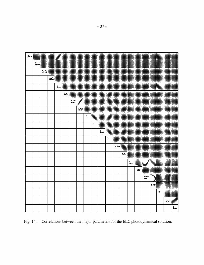
Fig. 14.— Correlations between the major parameters for the ELC photodynamical solution.

– 38 –

An alternative explanation for this tension may be found in the physical properties of thesecondary star. As discussed in Section 2.2, Kepler-1647 B is an active star with a rotation periodof 11 days. In addition, the residuals from the times of eclipse (Figure 4) provide evidence ofspots on the surface of this star, likely associated with strong magnetic fields. Such stellar activityis widely believed to be responsible for “radius inflation” among stars with convective envelopes(see, e.g. Torres 2013). The discrepancy between the measured and predicted radius for the radiusof Kepler-1647 B amounts to 0.014 R (1.4%), roughly 2.5 times the radius uncertainty at a fixedmass. Activity-induced radius inflation also generally causes the temperatures of late-type stars tobe too cool compared to model predictions. This “temperature suppression” is, however, not seenin the secondary star of Kepler-1647 possibly because of systematic errors in our spectroscopictemperatures or because the effect may be smaller than our uncertainties. We note that while radiusand temperature discrepancies are more commonly seen in M dwarfs, the secondary of Kepler-1647 is not unique in showing some of the same effects despite being much more massive (only∼3% less massive than the Sun). Other examples of active stars of similar mass as Kepler-1647 Bwith evidence of radius inflation and sometimes temperature suppression include V1061 Cyg B(Torres et al. 2006), CV Boo B (Torres et al. 2008), V636 Cen B (Clausen et al. 2009), and EF Aqr B(Vos et al. 2012). In some of these systems, the effect is substantially larger than that in Kepler-1647 B, and can reach up to 10%.

We note that while the best-fit apsidal constant for the primary star is consistent with the cor-responding models of Claret et al. (2006) within one sigma17 (i.e. k2(A,ELC) = 0.003±0.005 vsk2(A,Claret,M= 1.2 M)= 0.004), the nominal uncertainties on the secondary’s constant indicatea tension (i.e. k2(B,ELC) = 0.03±0.0005 vs k2(B,Claret,M = 1.0 M) = 0.015). To evaluate thesignificance of this tension on our results, we repeat the ELC fitting as described in the previoussection, but fixing the apsidal constants to those from Claret et al. (2006), i.e. k2(A) = 0.004 andk2(B) = 0.015. The fixed-constants solution is well within one sigma of the solution presented inTables 3 and 4 (where the constants are fit for), and the planet’s mass remains virtually unchanged,i.e. Mp(best−fit,fixed k2) = 462±167 MEarth vs Mp(best−fit, free k2) = 483±206 MEarth.

5.2. The Circumbinary Planet

Prior to the discovery of Kepler-1647b, all the known Kepler CBPs were Saturn-sized andsmaller (the largest being Kepler-34b, with a radius of 0.76 RJup), and were found to orbit theirhost binaries within a factor of two from their corresponding boundary for dynamical stability.Interestingly, “Jupiter-mass CBPs are likely to be less common because of their less stable evolu-

17For 4.4 Gyr, and Z = 0.01 – closest to the derived age and metallicity of Kepler-1647.

– 39 –

Fig. 15.— Radii (top panel) and temperatures (bottom) of the Kepler-1647 components as a func-tion of mass, compared with stellar evolution models from the Yonsei-Yale series (Yi et al. 2001;Demarque et al. 2004). Model isochrones are shown for the best-fit metallicity of [m/H] =−0.14and ages of 4.0–4.8 Gyr in steps of 0.1 Gyr, with the solid line marking the best-fit age of 4.4 Gyr.The insets in the top panel show enlargements around the primary and secondary observations.

– 40 –

Fig. 16.— Measurements for Kepler-1647 in the logg–Teff plane, along with 4.4 Gyr evolutionarytracks from the Yonsei-Yale series calculated for the measured masses and a metallicity of [m/H] =

−0.14. The shaded area around each track indicates the uncertainty in its location stemming fromthe mass errors. The left track is for the primary star, the right track for the secondary star.

– 41 –

tion”, suggest PN08, and “if present [Jupiter-mass CBPs] are likely to orbit at large distances fromthe central binary.”. Indeed – at the time of writing, with a radius of 1.06±0.01 RJup (11.8739±0.1377 REarth) and mass of 1.52±0.65 MJup (483±206 MEarth)18, Kepler-1647b is the first Joviantransiting CBP from Kepler , and the one with the longest orbital period (Pp = 1107.6 days).The size and the mass of the planet are consistent with theoretical predictions indicating thatsubstellar-mass objects evolve towards the radius of Jupiter after ∼ 1 Gyr of evolution for a widerange of initial masses (∼ 0.5− 10 MJup), and regardless of the initial conditions (‘hot’ or ‘cold’start) (Burrows et al. 2001, Spiegel & Burrows 2013). To date, Kepler-1647b is also one of thelongest-period transiting planets, demonstrating yet again the discovery potential of continuous,long-duration observations such as those made by Kepler. The orbit of the planet is nearly edge-on(ip = 90.0972± 0.0035), with a semi-major axis ap = 2.7205± 0.0070 AU and eccentricity ofep = 0.0581±0.0689.

5.3. Orbital Stability and Long-term Dynamics

Using Equation 3 from Holman & Weigert (1999) (also see Dvorak 1986, Dvorak et al. 1989),the boundary for orbital stability around Kepler-1647 is at acrit = 2.91 abin. With a semi-majoraxis of 2.72 AU (21.3 abin), Kepler-1647b is well beyond this stability limit indicating that theorbit of the planet is long-term stable. To confirm this, we also integrated the planet-binary systemusing the best-fit ELC parameters for a timescale of 100 million years. The results are shownin Figure 17. As seen from the figure, the semi-major axis and eccentricity of the planet do notexperience appreciable variations (that would inhibit the overall orbital stability of its orbit) overthe course of the integration.

On a shorter timescale, our numerical integration indicate that the orbital planes of the binaryand the planet undergo a 7040.87-years, anti-correlated precession in the plane of the sky. This isillustrated in Figure 18. As a result of this precession, the orbital inclinations of the binary andthe planet oscillate by∼ 0.0372 and∼ 2.9626, respectively (see upper and middle panels in Fig-ure 18). The mutual inclination between the planet and the binary star oscillates by∼ 0.0895, andthe planet’s ascending node varies by ∼ 2.9665 (see middle and lower left panels in Figure 17).

Taking into account the radii of the binary stars and planet, we found that CBP transits arepossible only if the planet’s inclination varies between 89.8137 and 90.1863. This transit windowis represented by the red horizontal lines in the middle panel of Figure 18. The planet can crossthe disks of the two stars only when the inclination of its orbit lies between these two lines. To

18See also Table 4 for mean and mode.

– 42 –

demonstrate this, in the lower panel of Figure 18 we expand the vertical scale near 90 degrees, andalso show the impact parameter b for the planet with respect to the primary (solid green symbols)and secondary (open blue symbols). Transits only formally occur when the impact parameter,relative to the sum of the stellar and planetary radii, is less than unity. We computed the impactparameter at the times of transit as well as at every conjunction, where a conjunction is deemedto have occurred if the projected separation of the planet and star is less than 5 planet radii alongthe x-coordinate19. Monitoring the impact parameter at conjunction allowed us to better determinethe time span for which transits are possible as shown in Figure 18. These transit windows, boundbetween the horizontal red lines in Figure 18, span about 204 years each. As a result, over oneprecession cycle, planetary transits can occur for≈ 408 years (spanning two transit windows, half aprecession cycle apart), i.e.,≈ 5.8% of the time. The transits of the CBP will cease in∼ 160 years.

Following the methods described in Welsh et al. (2012), we used the probability of transitfor Kepler-1647b to roughly estimate the frequency of Kepler-1647 -like systems. At the presentepoch, the transit probability is approximately 1/300 (i.e., RA/ap ∼ 0.33%), where the enhance-ment due to the barycentric motion of an aligned primary star is a minimal (∼ 5%) effect. Foldingin the probability of detecting two transits at two consecutive conjunctions of an 1100-day periodplanet when observing for 1400-days (i.e., 300/1400, or ∼ 20%), the probability of detectingKepler-1647b is therefore about 0.33%× 20%, or approximately 1/1500. Given that 1 such sys-tem was found out of Kepler’s ∼ 150,000 targets, this suggests an occurrence rate of roughly1%. A similar argument can be used to analyze the frequency among Eclipsing Binaries in par-ticular. As the population of EBs is already nearly aligned to the line-of-sight, the probabilityof alignment for the CBP is significantly increased. In particular, as described in Welsh et al.(2012), the probability that the planet will be aligned given that the target is an EB is approxi-mately abin/ap = 0.046 (compared to ∼ 0.003 for the isotropic case). Recent results suggest thatonly EBs with periods longer than ∼ 7 days contain CBPs (Welsh et al. 2013; Martin et al. 2015;Munoz & Lai 2015, Hamers et al. 2015); there are ∼ 1000 such Kepler EBs (Kirk et al. 2015).Thus, if 1% of these 1000 EBs have Kepler-1647-like CBPs, then the expected number of detec-tions would be 0.02×1000×0.046 = 0.92≈ 1. As a result, the Kepler-1647 system suggests that∼ 2% of all eligible EBs have similar planets.

Cumming et al. (2008) suggest a ∼ 1% occurrence rate of Jupiter mass planets within the 2-3AU range. Therefore, the relative frequency of such planets around FGK main sequence stars issimilar for both single and binary stars. This interesting result is consistent with what has beenfound for other CBPs as well and certainly has implications for planet formation theories. A moredetailed analysis following the methods of Armstrong et al. (2014) and Martin & Triaud (2015) in

19The xy-coordinates define the plane of the sky, and the observer is along the z-coordinate.

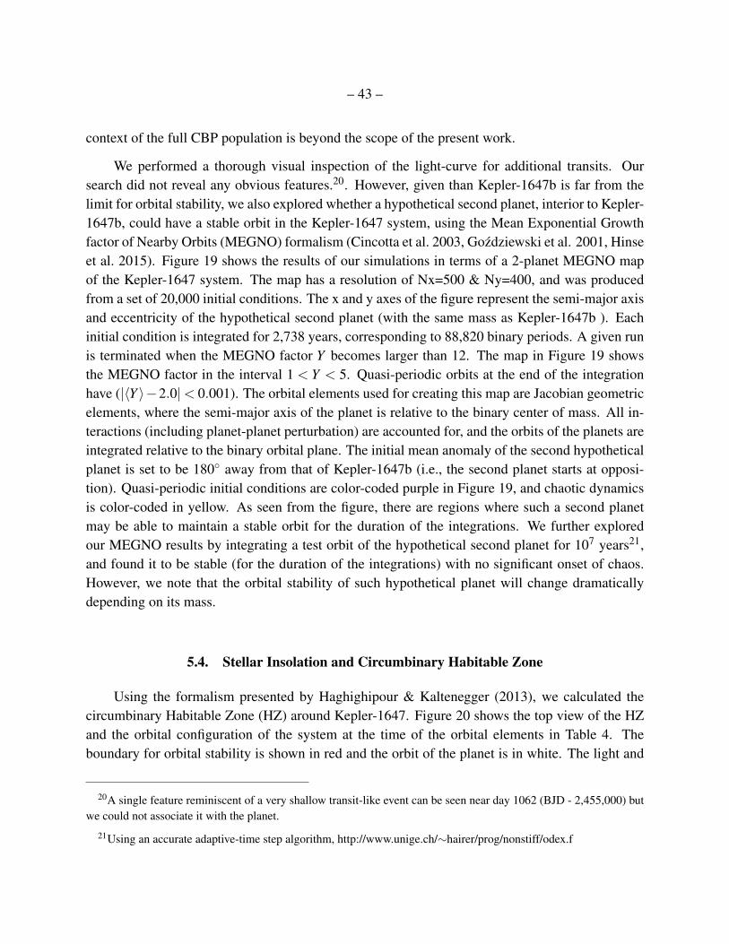
– 43 –

context of the full CBP population is beyond the scope of the present work.

We performed a thorough visual inspection of the light-curve for additional transits. Oursearch did not reveal any obvious features.20. However, given than Kepler-1647b is far from thelimit for orbital stability, we also explored whether a hypothetical second planet, interior to Kepler-1647b, could have a stable orbit in the Kepler-1647 system, using the Mean Exponential Growthfactor of Nearby Orbits (MEGNO) formalism (Cincotta et al. 2003, Gozdziewski et al. 2001, Hinseet al. 2015). Figure 19 shows the results of our simulations in terms of a 2-planet MEGNO mapof the Kepler-1647 system. The map has a resolution of Nx=500 & Ny=400, and was producedfrom a set of 20,000 initial conditions. The x and y axes of the figure represent the semi-major axisand eccentricity of the hypothetical second planet (with the same mass as Kepler-1647b ). Eachinitial condition is integrated for 2,738 years, corresponding to 88,820 binary periods. A given runis terminated when the MEGNO factor Y becomes larger than 12. The map in Figure 19 showsthe MEGNO factor in the interval 1 < Y < 5. Quasi-periodic orbits at the end of the integrationhave (|〈Y 〉−2.0|< 0.001). The orbital elements used for creating this map are Jacobian geometricelements, where the semi-major axis of the planet is relative to the binary center of mass. All in-teractions (including planet-planet perturbation) are accounted for, and the orbits of the planets areintegrated relative to the binary orbital plane. The initial mean anomaly of the second hypotheticalplanet is set to be 180 away from that of Kepler-1647b (i.e., the second planet starts at opposi-tion). Quasi-periodic initial conditions are color-coded purple in Figure 19, and chaotic dynamicsis color-coded in yellow. As seen from the figure, there are regions where such a second planetmay be able to maintain a stable orbit for the duration of the integrations. We further exploredour MEGNO results by integrating a test orbit of the hypothetical second planet for 107 years21,and found it to be stable (for the duration of the integrations) with no significant onset of chaos.However, we note that the orbital stability of such hypothetical planet will change dramaticallydepending on its mass.

5.4. Stellar Insolation and Circumbinary Habitable Zone

Using the formalism presented by Haghighipour & Kaltenegger (2013), we calculated thecircumbinary Habitable Zone (HZ) around Kepler-1647. Figure 20 shows the top view of the HZand the orbital configuration of the system at the time of the orbital elements in Table 4. Theboundary for orbital stability is shown in red and the orbit of the planet is in white. The light and

20A single feature reminiscent of a very shallow transit-like event can be seen near day 1062 (BJD - 2,455,000) butwe could not associate it with the planet.

21Using an accurate adaptive-time step algorithm, http://www.unige.ch/∼hairer/prog/nonstiff/odex.f

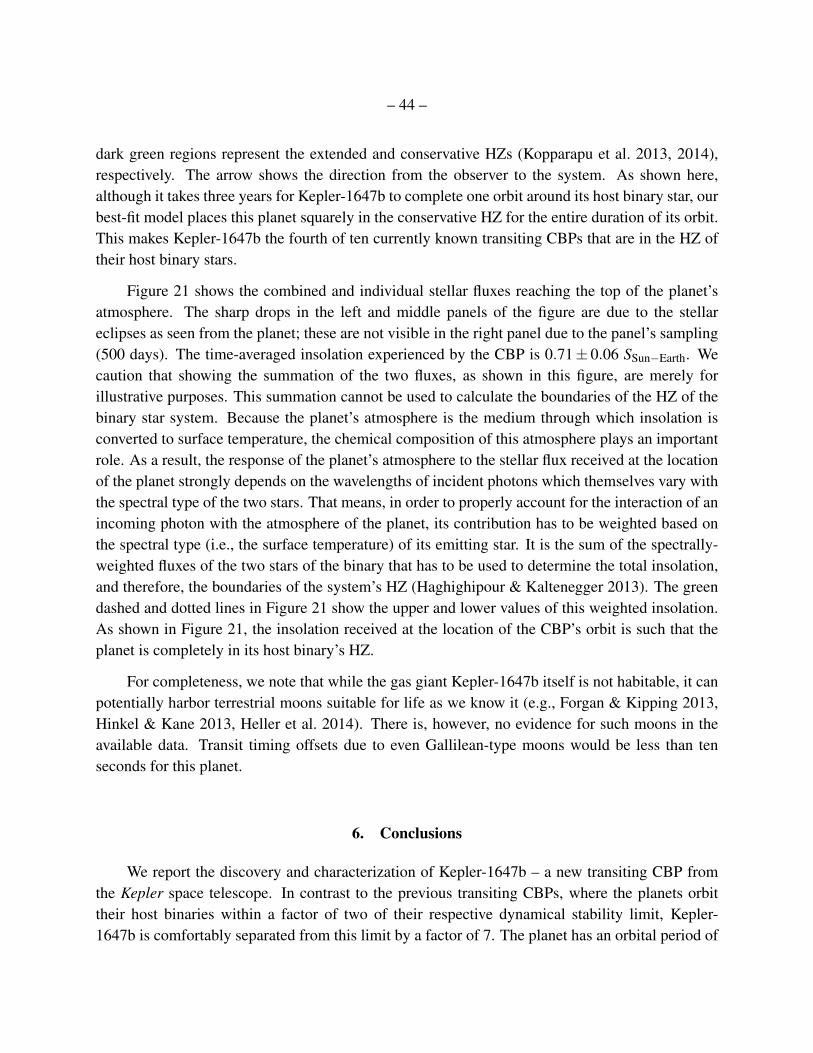
– 44 –

dark green regions represent the extended and conservative HZs (Kopparapu et al. 2013, 2014),respectively. The arrow shows the direction from the observer to the system. As shown here,although it takes three years for Kepler-1647b to complete one orbit around its host binary star, ourbest-fit model places this planet squarely in the conservative HZ for the entire duration of its orbit.This makes Kepler-1647b the fourth of ten currently known transiting CBPs that are in the HZ oftheir host binary stars.

Figure 21 shows the combined and individual stellar fluxes reaching the top of the planet’satmosphere. The sharp drops in the left and middle panels of the figure are due to the stellareclipses as seen from the planet; these are not visible in the right panel due to the panel’s sampling(500 days). The time-averaged insolation experienced by the CBP is 0.71± 0.06 SSun−Earth. Wecaution that showing the summation of the two fluxes, as shown in this figure, are merely forillustrative purposes. This summation cannot be used to calculate the boundaries of the HZ of thebinary star system. Because the planet’s atmosphere is the medium through which insolation isconverted to surface temperature, the chemical composition of this atmosphere plays an importantrole. As a result, the response of the planet’s atmosphere to the stellar flux received at the locationof the planet strongly depends on the wavelengths of incident photons which themselves vary withthe spectral type of the two stars. That means, in order to properly account for the interaction of anincoming photon with the atmosphere of the planet, its contribution has to be weighted based onthe spectral type (i.e., the surface temperature) of its emitting star. It is the sum of the spectrally-weighted fluxes of the two stars of the binary that has to be used to determine the total insolation,and therefore, the boundaries of the system’s HZ (Haghighipour & Kaltenegger 2013). The greendashed and dotted lines in Figure 21 show the upper and lower values of this weighted insolation.As shown in Figure 21, the insolation received at the location of the CBP’s orbit is such that theplanet is completely in its host binary’s HZ.

For completeness, we note that while the gas giant Kepler-1647b itself is not habitable, it canpotentially harbor terrestrial moons suitable for life as we know it (e.g., Forgan & Kipping 2013,Hinkel & Kane 2013, Heller et al. 2014). There is, however, no evidence for such moons in theavailable data. Transit timing offsets due to even Gallilean-type moons would be less than tenseconds for this planet.

6. Conclusions

We report the discovery and characterization of Kepler-1647b – a new transiting CBP fromthe Kepler space telescope. In contrast to the previous transiting CBPs, where the planets orbittheir host binaries within a factor of two of their respective dynamical stability limit, Kepler-1647b is comfortably separated from this limit by a factor of 7. The planet has an orbital period of

– 45 –

∼1100 days and a radius of 1.06±0.01 RJup. At the time of writing, Kepler-1647b is the longest-period, largest transiting CBP, and is also one of the longest-period transiting planets. With 1.52±0.65 MJup, this CBP is massive enough to measurably perturb the times of the stellar eclipses.Kepler-1647b completed a single revolution during Kepler’s observations and transited three times,one of them as a syzygy. We note that the next group of four transits (starting around date BJD =2,458,314.5, or UT of 2018, July, 15, see Table 7) will fall within the operation timeframe of TESS.The orbit of this CBP is long-term stable, with a precession period of ∼ 7,040 years. Due to itsorbital configuration, Kepler-1647b can produce transits for only ≈ 5.8% of its precession cycle.Despite having an orbital period of three years, this planet is squarely in the conservative HZ of itsbinary star for the entire length of its orbit.

The stellar system consists of two stars with MA = 1.2207± 0.0112 M, RA = 1.7903±0.0055 R, and MB = 0.9678± 0.0039 M, RB = 0.9663± 0.0057 R on a nearly edge-on orbitwith an eccentricity of 0.1602±0.0004. The two stars have a flux ratio of FB/FA = 0.21±0.02, thesecondary is an active star with a rotation period of Prot = 11.23±0.01 days, and the binary is ina spin-synchronized state. The two stars have effective temperatures of TA,eff = 6210±100 K andTB,eff = 5770±125 K respectively, metallicity of [Fe/H] =−0.14±0.05, and age of 4.4±0.25 Gyr.

As important as a new discovery of a CBP is to indulge our basic human curiosity about distantworlds, its main significance is to expand our understanding of the inner workings of planetarysystems in the dynamically rich environments of close binary stars. The orbital parameters ofCBPs, for example, provide important new insight into the properties of protoplanetary disks andshed light on planetary formation and migration in the dynamically-challenging environments ofbinary stars. In particular, the observed orbit of Kepler-1647b lends strong support to the modelssuggesting that CBPs form at large distances from their host binaries and subsequently migrateeither as a result of planet-disk interaction, or planet-planet scattering (e.g., Pierens & Nelson 2013,Kley & Haghighipour 2014, 2015).

We thank the referee for the insightful comments that helped us improve this paper. We thankGibor Basri and Andrew Collier Cameron for helpful discussions regarding stellar activity, MichaelAbdul-Masih, Kyle Conroy and Andrej Prsa for discussing the photometric centroid shifts. Thisresearch used observations from the Kepler Mission, which is funded by NASA’s Science Mis-sion Directorate; the TRES instrument on the Fred L. Whipple Observatory 1.5-m telescope; theTull Coude Spectrograph on the McDonald Observatory 2.7-m Harlan J. Smith Telescope; theHIRES instrument on the W. M. Keck Observatory 10-m telescope; the HamSpec instrument onthe Lick Observatory 3.5-m Shane telescope; the WHIRC instrument on the WIYN 4-m telescope;the Swarthmore College Observatory 0.6-m telescope; the Canela’s Robotic Observatory 0.3-mtelescope. This research made use of the SIMBAD database, operated at CDS, Strasbourg, France;

– 46 –

data products from the Two Micron All Sky Survey (2MASS), the United Kingdom Infrared Tele-scope (UKIRT); the NASA exoplanet archive NexSci22 and the NASA Community Follow-UpObservation Program (CFOP) website, operated by the NASA Exoplanet Science Institute and theCalifornia Institute of Technology, under contract with NASA under the Exoplanet ExplorationProgram. VBK and BQ gratefully acknowledge support by an appointment to the NASA Postdoc-toral Program at the Goddard Space Flight Center and at the Ames Research Center, administeredby Oak Ridge Associated Universities through a contract with NASA. WFW, JAO, GW, and BQgratefully acknowledge support from NASA via grants NNX13AI76G and NNX14AB91G. NHacknowledges support from the NASA ADAP program under grant NNX13AF20G, and NASAPAST program grant NNX14AJ38G. TCH acknowledges support from KASI research grant 2015-1-850-04. Part of the numerical computations have been carried out using the SFI/HEA IrishCenter for High-End Computing (ICHEC) and the POLARIS computing cluster at the Korea As-tronomy and Space Science Institute (KASI). This work was performed in part under contractwith the Jet Propulsion Laboratory (JPL) funded by NASA through the Sagan Fellowship Programexecuted by the NASA Exoplanet Science Institute.

REFERENCES

Armstrong, D. J., Osborn, H. P., Brown, D. J. A. et al. 2014, MNRAS, 444, 1873

Bryson, S. T., Jenkins, J. M., Gilliland, R.L., et al. 2013, PASP, 125, 889

Bromley, B. C. & Kenyon, S. J. 2015, ApJ806, 98

Burrows, A., Hubbard, W. B., Lunine, J. I. et al. 2001, RvMP, 73, 719

Carter, J. A., et al., 2011, Science, 331, 562

Chavez, C. E, Georgakarakos, N., Prodan, S. et al. 2015, MNRAS, 446, 1283

Cincotta, P. M., Giordano, C. M. & Simo, C. 2003, Physica D, 182, 151

Claret, A. 2006, A&A, 453, 769

Clausen, J. V., Bruntt, H., Claret, A., et al. 2009, A&A, 502, 253

Demarque, P., Woo, J-H, Kim, Y-C, & Yi, S. K. 2004, ApJS, 155, 667

Deeg, H.-J.; Doyle, L.R.; Kozhevnikov, V.P. et al., 1998, A&A338, 479

22http://exoplanetarchive.ipac.caltech.edu

– 47 –

Doyle, L.R.; Deeg, H.-J.; Kozhevnikov, V.P., 2000, ApJ 535, 338

Doyle, L.R. & H-J. Deeg, 2004, “Timing Detection of Eclipsing Binary Planets and TransitingExtrasolar Moons”, in Bioastronomy 2002: Life Among the Stars, IAU Symposium 213,R.P Norris and F.H. Stootman (eds), A.S.P., San Francisco, CA, 80-84

Doyle, L. R.; Carter, J. A., Fabrycky, D. C., et al. 2011, Science, 333, 6049

Doyle, A. P., Davies, G. R., Smalley, B. et al. 2014, MNRAS, 444, 3592

Dressing, C. D.; Adams, E. R.; Dupree, A. K.; Kulesa, C.; McCarthy, D. 2014, AJ, 148, 78

Dvorak, R. 1986, A&A, 167, 379

Dvorak, R., Froeschle, C., & Froeschle, Ch. 1989, A&A, 226, 335

Eastman, J, Silverd, R. & Gaudi, S. B. 2010, PASP, 122, 935

Fabrycky, D. C. & Tremaine, S., 2007, ApJ, 669, 1289

Feroz F., Hobson M. P. & Bridges M., 2008, MNRAS384, 449

Foucart, F. and Lai, D., 2013, ApJ, 764, 106

Furesz, G. 2008, PhD thesis, Univ. of Szeged, Hungary

Gilliland, R. L.; Chaplin, W. J.; Dunham, E. W. et al., 2011, ApJS, 197, 6

Gozdziewski, K.,Bois, E., Maciejewski, A. J., and Kiseleva-Eggleton, L. 2001, A&A, 378, 569

Haghighipour, N. & Kaltenegger, L. 2013, ApJ, 777, 166

Hamers, A., Perets, H. B. & Portegies Zwart, S. 2015, arXiv:1506.02039

Hilditch, R. W. 2001, An Introduction to Close Binary Stars, by R. W. Hilditch, pp. 392. ISBN0521241065. Cambridge, UK: Cambridge University Press, March 2001.

Hinse, T. C., Lee, J. W., Gozdziewski, K. et al. 2014, MNRAS, 438, 307

Hinse, T. C., Haghighipour, N., Kostov, V. B & Gozdziewski, K., 2010, ApJ, 799, 88

Holman, M. J. & Wiegert, P. A., 1999, AJ, 117, 621

Holczer, T., Shporer, A., Mazeh, T. et al. 2015, ApJ, 870, 170

Hut, P. 1981, A&A, 99, 126

– 48 –

Hut, P. 1981, BAAS, 14, 902

Jenkins, J. M., Doyle, L.R., & Cullers, K., 1996, Icarus 119, 244

Kirk, B. et al. 2015, submitted

Kley, W. & Haghighipou, N. 2014, A&A, 564, 72

Kley, W. & Haghighipou, N. 2015, A&A, 581, 20

Koch, D. G., Borucki, W. J., Basri, G. et al. 2010, ApJ, 713, 79

Kopparapu, R. K.; Ramirez, R.; Kasting, J. F. et al. 2013, ApJ, 765, 2

Kolbl, R., Marcy, G. W., Isaacson, H. & Howard, A. W. 2015, AJ, 149, 18

Kostov, V. B.; McCullough, P. R.; Hinse, T. C., et al. 2013, ApJ, 770, 52

Kostov, V. B.; McCullough, P. R., Carter, J. A. et al., 2014, ApJ, 784, 14

Kovacs, G., Zucker, S., & Mazeh, T. 2002, A&A, 391, 369

Kozai, Y. 1962, AJ, 67, 591

Latham, D. W.; Stefanik, R. P., Torres, G. et al. 2002, AJ, 124, 1144

Lines, S., Leinhardt, Z. M., Baruteau, C. et al. 2015, A&A, 582, 5

Lawrence, A., et al.. 2007, MNRAS, 379, 1599

Mandel, K., & Agol, E. 2002, ApJ, 580, L171

R. A. Mardling, & D. N. C. Lin, 2002, ApJ, 573, 829

Martin, D. V. & Triaud, A. H. M. J. 2014, A&A, 570, 91

Martin, D. V. & Triaud, A. H. M. J. 2015, MNRAS, 449, 781

Martin, D. V.; Mazeh, T.; & Fabrycky, D. C. 2015, MNRAS, 453, 3554

Marzari, F.; Thebault, P.; Scholl, H., et al., 2013, A&A, 553, 71

Matijevic, G. et al., 2012, AJ, 143,123

Mazeh, T., & Shaham, J. 1979, A&A, 77, 145

Mazeh, T., Holczer, T. & Shporer, A. 2015, ApJ, 800, 142

– 49 –

McQuillan, A., Aigrain, S. & Mazeh, T. 2013, MNRAS, 432, 1203

McQuillan, A., Mazeh, T. & Aigrain, S. 2013, ApJ, 775, 11

Meixner, M., Smee, S., Doering, R. L., et al., 2010, PASP, 122, 890

Meschiari, S., 2013, eprint arXiv:1309.4679

Miranda, R. & Lai, D. 2015, MNRAS, 452, 2396

Murray, C. D. & Correia, A. C. M. 2011, Exoplanets, edited by S. Seager. Tucson, AZ: Universityof Arizona Press, 2011, 526 pp. ISBN 978-0-8165-2945-2., p.15-23

Nordstrom, B., Latham, D. W., Morse et al. 1994, A&A, 287, 338

Orosz, J. A. & Hauschildt, P. H. 2000, A&A, 364, 265

Orosz, J. A., Welsh, W. F., Carter, J. A., et al. 2012, Science, 337, 1511

Orosz, J. A., Welsh, W. F., Carter, J. A., et al. 2012, ApJ, 758, 87

Orosz, J. A. et al. 2015, submitted

Paardekooper, S.-J.; Leinhardt, Z. M.; Thbault, P.; Baruteau, C., 2012, ApJ, 754, 16

Pal, A., 2012, MNRAS, 420, 1630

Pelupessy, F. I. & Portegies Zwart, S. 2013, MNRAS, 429, 895

Prsa, A., Batalha, N., Slawson, R. W., et al. 2011, AJ, 141, 83

Pierens, A. & Nelson, R. P., 2007, A&A, 472, 993

Pierens, A. & Nelson, R. P., 2008, A&A, 483, 633

Pierens, A. & Nelson, R. P., 2008, A&A, 482, 333

Pierens, A. & Nelson, R. P., 2008, A&A, 478, 939

Pierens, A. & Nelson, R. P., 2013, A&A, 556, 134

Rafikov, R., 2013, ApJ, 764, 16

Raghavan, D.; McAlister, H. A.; Henry, T. J. et al., 2010, ApJS, 191, 1

Schneider, J., & Chevreton, M. 1990, A&A, 232, 251

– 50 –

Schneider, J., & Doyle, L. R. 1995, Earth, Moon, and Planets 71, 153

Schneider, J., 1994, P&SS, 42, 539

Schwamb, M. E., Orosz, J. A., Carter, J. A. et al. 2013, ApJ, 768, 127

Silsbee, K. & Rafikov, R. R. 2015, ApJ, 798, 71

Skilling J. 2004, in Fischer R., Preuss R., Toussaint U. V., eds, American Institute of PhysicsConference Series Nested Sampling, pp 395-405

Slawson, R. W., Prsa, A. Welsh, W. F. et al. 2011, AJ, 142, 160

Spiegel, D. S. & Burrows, A. 2013, ApJ, 772, 76

C. J. F. ter Braak, & J. A. Vrugt, J.A., A Markov Chain Monte Carlo version of the genetic algo-rithm Differential Evolution: easy Bayesian computing for real parameter spaces. Statisticsand Computing 16, 239–249 (2006).

Torres, G. 2013, Astronomische Nachrichten, 334, 4

Torres, G., Andersen, J., & Gimenez, A. 2010, A&A Rev., 18, 67

Torres, G., Lacy, C. H., Marschall, L. A., Sheets, H. A., & Mader, J. A. 2006, ApJ, 640, 1018

Torres, G., Vaz, L. P. R., & Sandberg Lacy, C. H. 2008, AJ, 136, 2158

Tull, R. G., MacQueen, P. J., Sneden, C. & Lambert, D. L. 1995, PASP, 107, 251

Vogt, S. S. 1987, PASP, 99, 1214

Vogt, S. S., Allen, S. L., Bigelow, B. C., et al. 1994, SPIE, 2198, 362

Vos, J., Clausen, J. V., Jrgensen, U. G., et al. 2012, A&A, 540, A64

Welsh, W. F.; Orosz, J. A.; Carter, J. A., et al. 2012, Nature, 481, 475

Welsh, W.F., Orosz, J.A., Carter, J.A. & Fabrycky, D.C., 2014, “Kepler Results On CircumbinaryPlanets”, in Formation, Detection, and Characterization of Extrasolar Habitable Planets,Proceedings of the International Astronomical Union, IAU Symposium, Volume 293, pp.125-132

Welsh, W. F. et al., 2015, ApJ, 809, 26

Winn, J. N. & Holman, M., 2005, ApJ, 628, 159

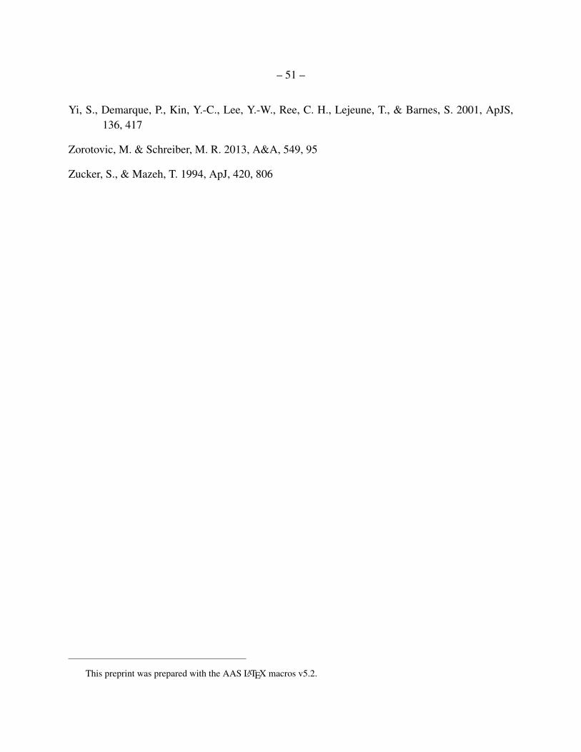
– 51 –

Yi, S., Demarque, P., Kin, Y.-C., Lee, Y.-W., Ree, C. H., Lejeune, T., & Barnes, S. 2001, ApJS,136, 417

Zorotovic, M. & Schreiber, M. R. 2013, A&A, 549, 95

Zucker, S., & Mazeh, T. 1994, ApJ, 420, 806

This preprint was prepared with the AAS LATEX macros v5.2.

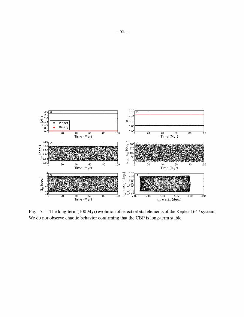
– 52 –

Fig. 17.— The long-term (100 Myr) evolution of select orbital elements of the Kepler-1647 system.We do not observe chaotic behavior confirming that the CBP is long-term stable.

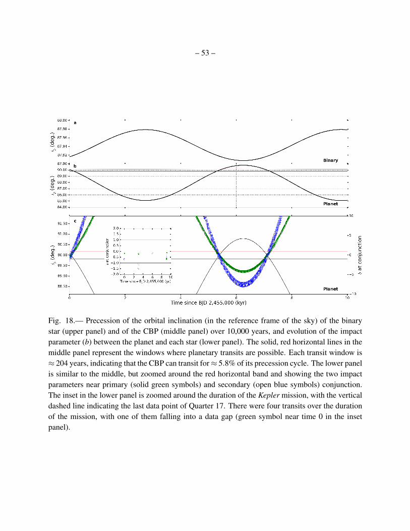
– 53 –

Fig. 18.— Precession of the orbital inclination (in the reference frame of the sky) of the binarystar (upper panel) and of the CBP (middle panel) over 10,000 years, and evolution of the impactparameter (b) between the planet and each star (lower panel). The solid, red horizontal lines in themiddle panel represent the windows where planetary transits are possible. Each transit window is≈ 204 years, indicating that the CBP can transit for≈ 5.8% of its precession cycle. The lower panelis similar to the middle, but zoomed around the red horizontal band and showing the two impactparameters near primary (solid green symbols) and secondary (open blue symbols) conjunction.The inset in the lower panel is zoomed around the duration of the Kepler mission, with the verticaldashed line indicating the last data point of Quarter 17. There were four transits over the durationof the mission, with one of them falling into a data gap (green symbol near time 0 in the insetpanel).

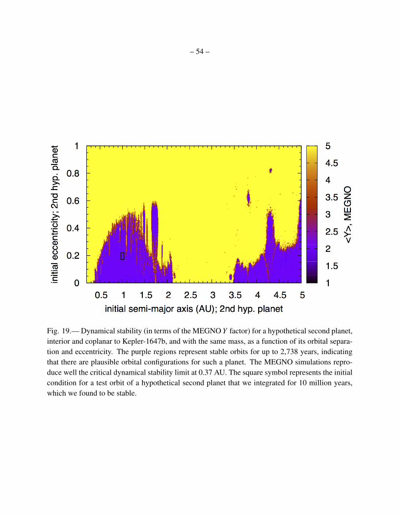
– 54 –

Fig. 19.— Dynamical stability (in terms of the MEGNO Y factor) for a hypothetical second planet,interior and coplanar to Kepler-1647b, and with the same mass, as a function of its orbital separa-tion and eccentricity. The purple regions represent stable orbits for up to 2,738 years, indicatingthat there are plausible orbital configurations for such a planet. The MEGNO simulations repro-duce well the critical dynamical stability limit at 0.37 AU. The square symbol represents the initialcondition for a test orbit of a hypothetical second planet that we integrated for 10 million years,which we found to be stable.

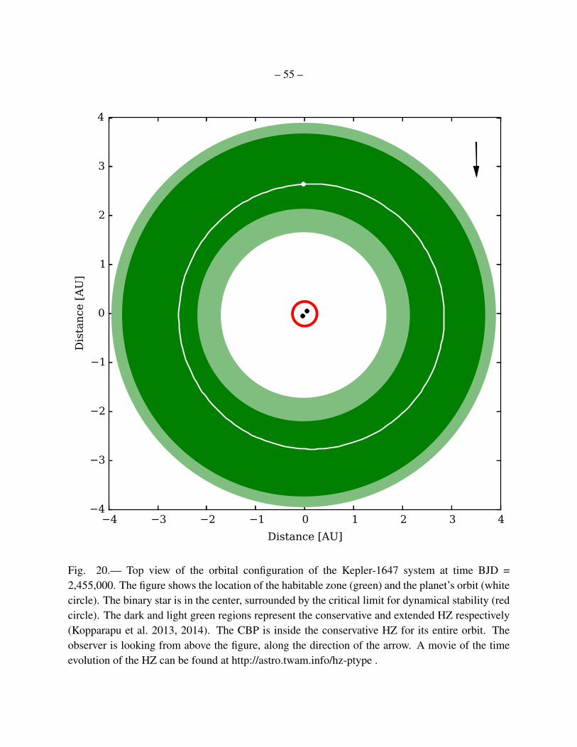
– 55 –

Fig. 20.— Top view of the orbital configuration of the Kepler-1647 system at time BJD =2,455,000. The figure shows the location of the habitable zone (green) and the planet’s orbit (whitecircle). The binary star is in the center, surrounded by the critical limit for dynamical stability (redcircle). The dark and light green regions represent the conservative and extended HZ respectively(Kopparapu et al. 2013, 2014). The CBP is inside the conservative HZ for its entire orbit. Theobserver is looking from above the figure, along the direction of the arrow. A movie of the timeevolution of the HZ can be found at http://astro.twam.info/hz-ptype .

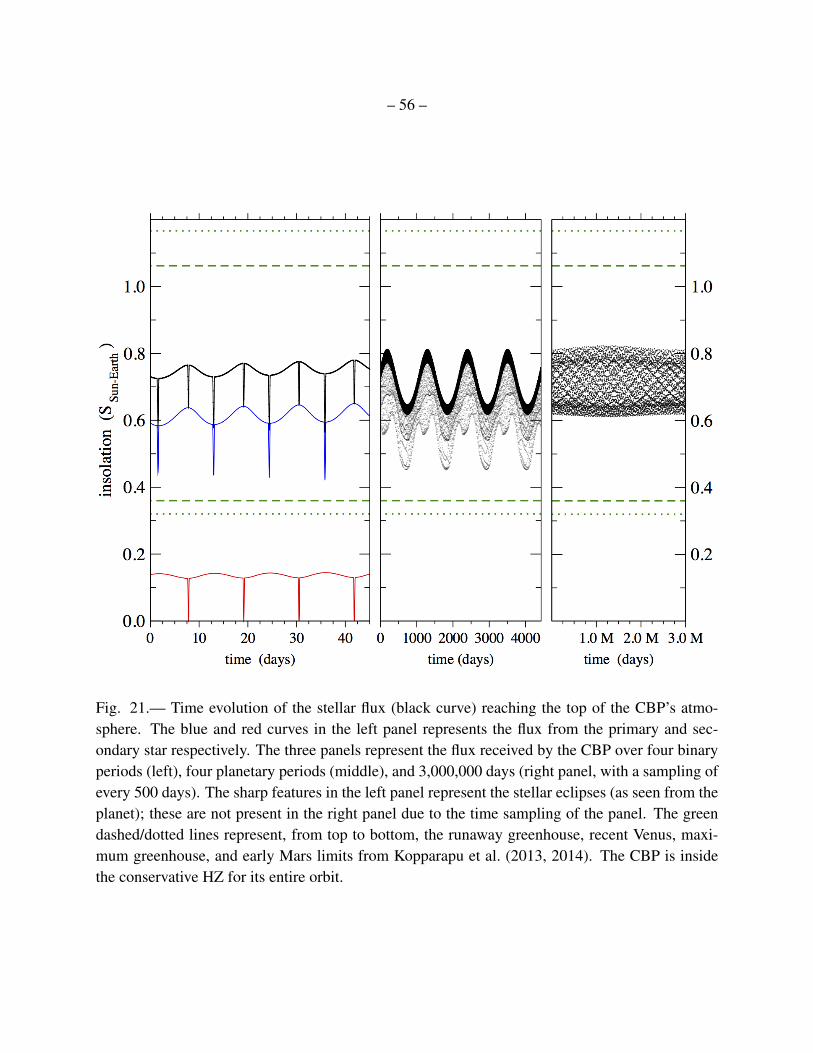
– 56 –

Fig. 21.— Time evolution of the stellar flux (black curve) reaching the top of the CBP’s atmo-sphere. The blue and red curves in the left panel represents the flux from the primary and sec-ondary star respectively. The three panels represent the flux received by the CBP over four binaryperiods (left), four planetary periods (middle), and 3,000,000 days (right panel, with a sampling ofevery 500 days). The sharp features in the left panel represent the stellar eclipses (as seen from theplanet); these are not present in the right panel due to the time sampling of the panel. The greendashed/dotted lines represent, from top to bottom, the runaway greenhouse, recent Venus, maxi-mum greenhouse, and early Mars limits from Kopparapu et al. (2013, 2014). The CBP is insidethe conservative HZ for its entire orbit.

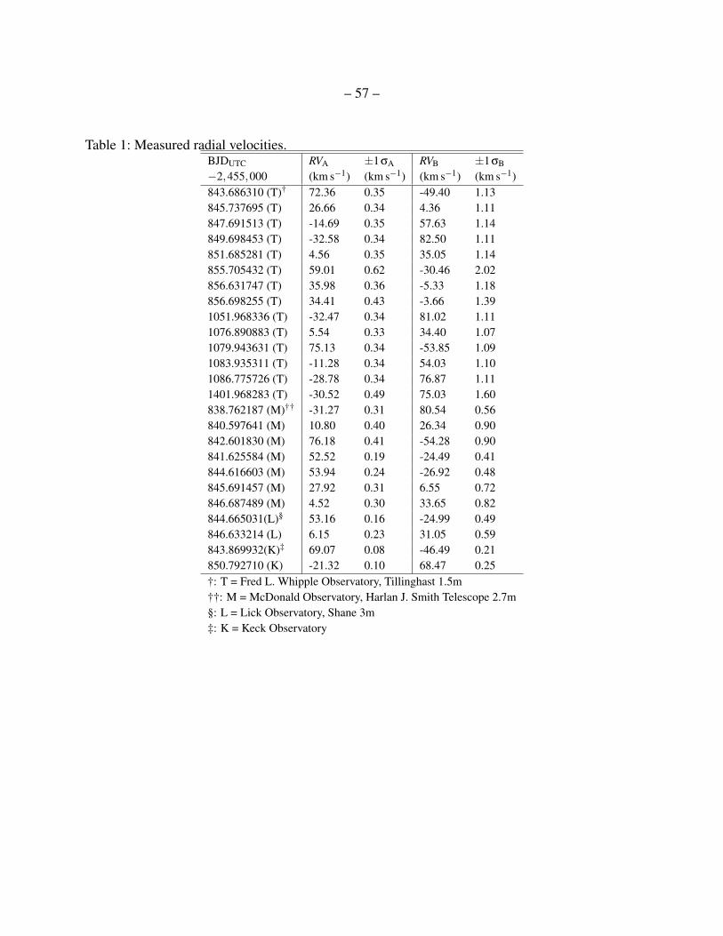
– 57 –

Table 1: Measured radial velocities.BJDUTC RVA ±1σA RVB ±1σB

−2,455,000 (km s−1) (km s−1) (km s−1) (km s−1)843.686310 (T)† 72.36 0.35 -49.40 1.13845.737695 (T) 26.66 0.34 4.36 1.11847.691513 (T) -14.69 0.35 57.63 1.14849.698453 (T) -32.58 0.34 82.50 1.11851.685281 (T) 4.56 0.35 35.05 1.14855.705432 (T) 59.01 0.62 -30.46 2.02856.631747 (T) 35.98 0.36 -5.33 1.18856.698255 (T) 34.41 0.43 -3.66 1.391051.968336 (T) -32.47 0.34 81.02 1.111076.890883 (T) 5.54 0.33 34.40 1.071079.943631 (T) 75.13 0.34 -53.85 1.091083.935311 (T) -11.28 0.34 54.03 1.101086.775726 (T) -28.78 0.34 76.87 1.111401.968283 (T) -30.52 0.49 75.03 1.60838.762187 (M)†† -31.27 0.31 80.54 0.56840.597641 (M) 10.80 0.40 26.34 0.90842.601830 (M) 76.18 0.41 -54.28 0.90841.625584 (M) 52.52 0.19 -24.49 0.41844.616603 (M) 53.94 0.24 -26.92 0.48845.691457 (M) 27.92 0.31 6.55 0.72846.687489 (M) 4.52 0.30 33.65 0.82844.665031(L)§ 53.16 0.16 -24.99 0.49846.633214 (L) 6.15 0.23 31.05 0.59843.869932(K)‡ 69.07 0.08 -46.49 0.21850.792710 (K) -21.32 0.10 68.47 0.25†: T = Fred L. Whipple Observatory, Tillinghast 1.5m††: M = McDonald Observatory, Harlan J. Smith Telescope 2.7m§: L = Lick Observatory, Shane 3m‡: K = Keck Observatory

– 58 –

Table 2: Kepler-1647 : the Eclipsing BinaryParameter Value Uncertainty (1σ) Unit NoteOrbital Period, Pbin 11.25882 0.00060 days Prsa et al. (2011)Epoch of Periastron passage, T0 -47.86903 0.00267 days† SpectroscopyVelocity semi-amplitude, KA 55.73 0.21 km s−1 SpectroscopyVelocity semi-amplitude, KB 69.13 0.50 km s−1 SpectroscopySystem velocity offset, γ 18.00 0.13 km s−1 SpectroscopyEccentricity, ebin 0.1593 0.0030 SpectroscopyArgument of Periapsis, ωbin 300.85 0.91 SpectroscopySemi-major Axis, aA sin i 12.24 0.04 R SpectroscopySemi-major Axis, aB sin i 15.19 0.11 R SpectroscopySemi-major Axis, abin sin i 27.43 0.12 R SpectroscopyMass of star A, MA sin3 i 1.210 0.019 M SpectroscopyMass of star B, MB sin3 i 0.975 0.010 M SpectroscopyMass ratio, Q = MB/MA 0.8062 0.0063 SpectroscopyTemperature of Star A, TA 6210 100 K SpectroscopyTemperature of Star B, TB 5770 125 K SpectroscopyFlux ratio, FB/FA 0.21 0.02 SpectroscopyV sin i of Star A, V sin i 8.4 0.5 km s−1 SpectroscopyV sin i of Star B, V sin i 5.1 1.0 km s−1 SpectroscopyFe/H of Star A, [Fe/H] -0.14 0.05 SpectroscopyAge 4.4 0.25 Gyr SpectroscopyNormalized Semi-major Axis, RA/abin 0.0655 0.0002 Photometry††

Normalized Semi-major Axis, RB/abin 0.0354 0.0001 PhotometryFlux ratio, FB/FA 0.22 0.02 PhotometryFlux Contamination Fcont,imaging 0.069 0.015 PhotometryFlux Contamination (mean), Fcont,MAST 0.04 0.01 MAST

†: BJD - 2,455,000††: Based on pre-photodynamic analysis of the Kepler data.

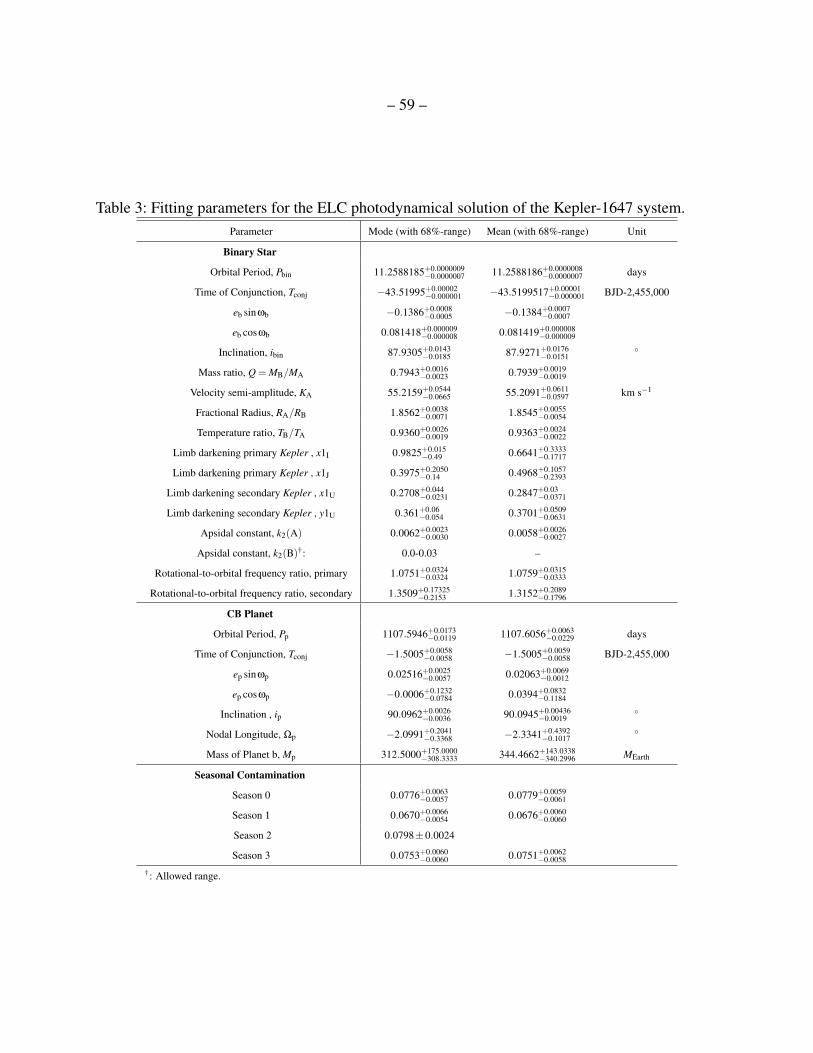
– 59 –

Table 3: Fitting parameters for the ELC photodynamical solution of the Kepler-1647 system.Parameter Mode (with 68%-range) Mean (with 68%-range) Unit

Binary Star

Orbital Period, Pbin 11.2588185+0.0000009−0.0000007 11.2588186+0.0000008

−0.0000007 days

Time of Conjunction, Tconj −43.51995+0.00002−0.000001 −43.5199517+0.00001

−0.000001 BJD-2,455,000

eb sinωb −0.1386+0.0008−0.0005 −0.1384+0.0007

−0.0007

eb cosωb 0.081418+0.000009−0.000008 0.081419+0.000008

−0.000009

Inclination, ibin 87.9305+0.0143−0.0185 87.9271+0.0176

−0.0151

Mass ratio, Q = MB/MA 0.7943+0.0016−0.0023 0.7939+0.0019

−0.0019

Velocity semi-amplitude, KA 55.2159+0.0544−0.0665 55.2091+0.0611

−0.0597 km s−1

Fractional Radius, RA/RB 1.8562+0.0038−0.0071 1.8545+0.0055

−0.0054

Temperature ratio, TB/TA 0.9360+0.0026−0.0019 0.9363+0.0024

−0.0022

Limb darkening primary Kepler , x1I 0.9825+0.015−0.49 0.6641+0.3333

−0.1717

Limb darkening primary Kepler , x1J 0.3975+0.2050−0.14 0.4968+0.1057

−0.2393

Limb darkening secondary Kepler , x1U 0.2708+0.044−0.0231 0.2847+0.03

−0.0371

Limb darkening secondary Kepler , y1U 0.361+0.06−0.054 0.3701+0.0509

−0.0631

Apsidal constant, k2(A) 0.0062+0.0023−0.0030 0.0058+0.0026

−0.0027

Apsidal constant, k2(B)†: 0.0-0.03 –

Rotational-to-orbital frequency ratio, primary 1.0751+0.0324−0.0324 1.0759+0.0315

−0.0333

Rotational-to-orbital frequency ratio, secondary 1.3509+0.17325−0.2153 1.3152+0.2089

−0.1796

CB Planet

Orbital Period, Pp 1107.5946+0.0173−0.0119 1107.6056+0.0063

−0.0229 days

Time of Conjunction, Tconj −1.5005+0.0058−0.0058 −1.5005+0.0059

−0.0058 BJD-2,455,000

ep sinωp 0.02516+0.0025−0.0057 0.02063+0.0069

−0.0012

ep cosωp −0.0006+0.1232−0.0784 0.0394+0.0832

−0.1184

Inclination , ip 90.0962+0.0026−0.0036 90.0945+0.00436

−0.0019

Nodal Longitude, Ωp −2.0991+0.2041−0.3368 −2.3341+0.4392

−0.1017

Mass of Planet b, Mp 312.5000+175.0000−308.3333 344.4662+143.0338

−340.2996 MEarth

Seasonal Contamination

Season 0 0.0776+0.0063−0.0057 0.0779+0.0059

−0.0061

Season 1 0.0670+0.0066−0.0054 0.0676+0.0060

−0.0060

Season 2 0.0798±0.0024

Season 3 0.0753+0.0060−0.0060 0.0751+0.0062

−0.0058

†: Allowed range.

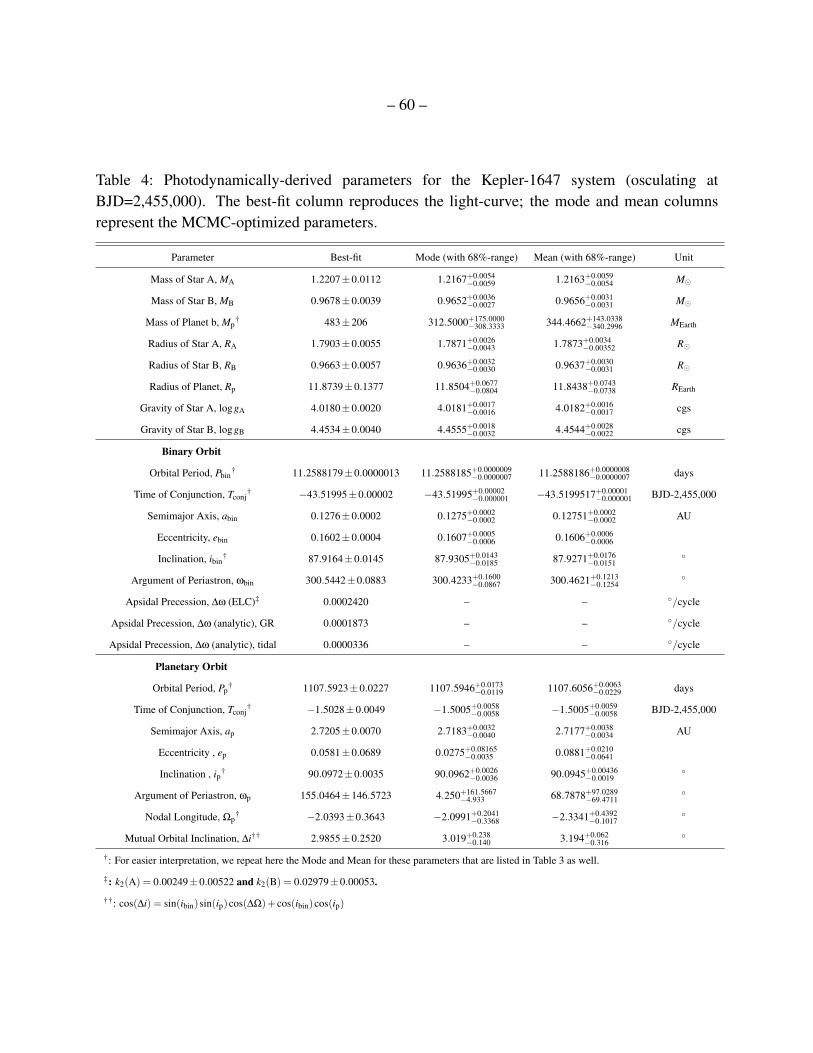
– 60 –

Table 4: Photodynamically-derived parameters for the Kepler-1647 system (osculating atBJD=2,455,000). The best-fit column reproduces the light-curve; the mode and mean columnsrepresent the MCMC-optimized parameters.

Parameter Best-fit Mode (with 68%-range) Mean (with 68%-range) Unit

Mass of Star A, MA 1.2207±0.0112 1.2167+0.0054−0.0059 1.2163+0.0059

−0.0054 M

Mass of Star B, MB 0.9678±0.0039 0.9652+0.0036−0.0027 0.9656+0.0031

−0.0031 M

Mass of Planet b, Mp† 483±206 312.5000+175.0000

−308.3333 344.4662+143.0338−340.2996 MEarth

Radius of Star A, RA 1.7903±0.0055 1.7871+0.0026−0.0043 1.7873+0.0034

−0.00352 R

Radius of Star B, RB 0.9663±0.0057 0.9636+0.0032−0.0030 0.9637+0.0030

−0.0031 R

Radius of Planet, Rp 11.8739±0.1377 11.8504+0.0677−0.0804 11.8438+0.0743

−0.0738 REarth

Gravity of Star A, loggA 4.0180±0.0020 4.0181+0.0017−0.0016 4.0182+0.0016

−0.0017 cgs

Gravity of Star B, loggB 4.4534±0.0040 4.4555+0.0018−0.0032 4.4544+0.0028

−0.0022 cgs

Binary Orbit

Orbital Period, Pbin† 11.2588179±0.0000013 11.2588185+0.0000009

−0.0000007 11.2588186+0.0000008−0.0000007 days

Time of Conjunction, Tconj† −43.51995±0.00002 −43.51995+0.00002

−0.000001 −43.5199517+0.00001−0.000001 BJD-2,455,000

Semimajor Axis, abin 0.1276±0.0002 0.1275+0.0002−0.0002 0.12751+0.0002

−0.0002 AU

Eccentricity, ebin 0.1602±0.0004 0.1607+0.0005−0.0006 0.1606+0.0006

−0.0006

Inclination, ibin† 87.9164±0.0145 87.9305+0.0143

−0.0185 87.9271+0.0176−0.0151

Argument of Periastron, ωbin 300.5442±0.0883 300.4233+0.1600−0.0867 300.4621+0.1213

−0.1254

Apsidal Precession, ∆ω (ELC)‡ 0.0002420 – – /cycle

Apsidal Precession, ∆ω (analytic), GR 0.0001873 – – /cycle

Apsidal Precession, ∆ω (analytic), tidal 0.0000336 – – /cycle

Planetary Orbit

Orbital Period, Pp† 1107.5923±0.0227 1107.5946+0.0173

−0.0119 1107.6056+0.0063−0.0229 days

Time of Conjunction, Tconj† −1.5028±0.0049 −1.5005+0.0058

−0.0058 −1.5005+0.0059−0.0058 BJD-2,455,000

Semimajor Axis, ap 2.7205±0.0070 2.7183+0.0032−0.0040 2.7177+0.0038

−0.0034 AU

Eccentricity , ep 0.0581±0.0689 0.0275+0.08165−0.0035 0.0881+0.0210

−0.0641

Inclination , ip† 90.0972±0.0035 90.0962+0.0026−0.0036 90.0945+0.00436

−0.0019

Argument of Periastron, ωp 155.0464±146.5723 4.250+161.5667−4.933 68.7878+97.0289

−69.4711

Nodal Longitude, Ωp† −2.0393±0.3643 −2.0991+0.2041

−0.3368 −2.3341+0.4392−0.1017

Mutual Orbital Inclination, ∆i†† 2.9855±0.2520 3.019+0.238−0.140 3.194+0.062

−0.316

†: For easier interpretation, we repeat here the Mode and Mean for these parameters that are listed in Table 3 as well.

‡: k2(A) = 0.00249±0.00522 and k2(B) = 0.02979±0.00053.

††: cos(∆i) = sin(ibin)sin(ip)cos(∆Ω)+ cos(ibin)cos(ip)

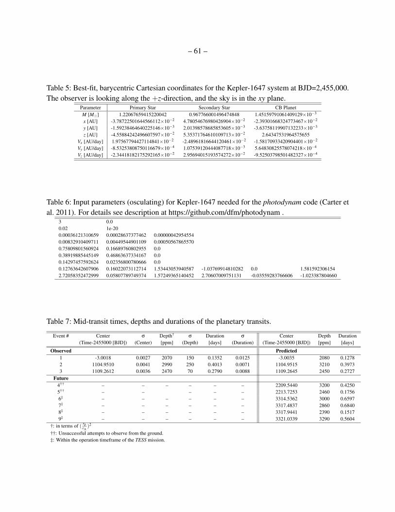
– 61 –

Table 5: Best-fit, barycentric Cartesian coordinates for the Kepler-1647 system at BJD=2,455,000.The observer is looking along the +z-direction, and the sky is in the xy plane.

Parameter Primary Star Secondary Star CB PlanetM [M] 1.22067659415220042 0.967766001496474848 1.45159791061409129×10−3

x [AU] -3.78722501644566112×10−2 4.78054676980426904×10−2 -2.39301668324773467×10−2

y [AU] -1.59238464640225146×10−3 2.01398578685853605×10−3 -3.63758119907132233×10−3

z [AU] -4.55884242496607597×10−2 5.35371764610109713×10−2 2.64347531964575655Vx [AU/day] 1.97567794427114841×10−2 -2.48961816644120461×10−2 -1.58170933420904401×10−2

Vy [AU/day] -8.53253808750116679×10−4 1.07539120444087718×10−3 5.64830825578074218×10−4

Vz [AU/day] -2.34418182175292165×10−2 2.95694015193574272×10−2 -9.52503798501482327×10−4

Table 6: Input parameters (osculating) for Kepler-1647 needed for the photodynam code (Carter etal. 2011). For details see description at https://github.com/dfm/photodynam .

3 0.00.02 1e-200.00036121310659 0.00028637377462 0.000000429545540.00832910409711 0.00449544901109 0.000505678655700.75809801560924 0.16689760802955 0.00.38919885445149 0.46863637334167 0.00.14297457592624 0.02356800780666 0.00.12763642607906 0.16022073112714 1.53443053940587 -1.03769914810282 0.0 1.5815923061542.72058352472999 0.05807789749374 1.57249365140452 2.70607009751131 -0.03559283766606 -1.023387804660

Table 7: Mid-transit times, depths and durations of the planetary transits.

Event # Center σ Depth† σ Duration σ Center Depth Duration(Time-2455000 [BJD]) (Center) [ppm] (Depth) [days] (Duration) (Time-2455000 [BJD]) [ppm] [days]

Observed Predicted1 -3.0018 0.0027 2070 150 0.1352 0.0125 -3.0035 2080 0.12782 1104.9510 0.0041 2990 250 0.4013 0.0071 1104.9515 3210 0.39733 1109.2612 0.0036 2470 70 0.2790 0.0088 1109.2645 2450 0.2727

Future4†† – – – – – – 2209.5440 3200 0.42505†† – – – – – 2213.7253 2460 0.17566‡ – – – – – – 3314.5362 3000 0.65977‡ – – – – – – 3317.4837 2860 0.68408‡ – – – – – – 3317.9441 2390 0.15179‡ – – – – – – 3321.0339 3290 0.5604

†: in terms of ( rprA)2

††: Unsuccessful attempts to observe from the ground.‡: Within the operation timeframe of the TESS mission.