Gaussian Orbital Determination of 1943 Anteros

1Gaussian Orbital Determination of 1943 AnterosMatthew Li, Zoey Flynn, Jonathan Heckerman

Summer Science Program 2014

Abstract – Over the course of about six weeks, aseries of images was taken of the near-earth asteroid1943 Anteros. Data from these images were analyzed inorder to determine the orbit of the asteroid and the riskof a collision with Earth in the future. Results revealedthat Anteros has a semi-major axis of approximately1.44 AU, an eccentricity of 0.26, and an inclination of8.71. The longitude of the ascending node is 246.2,the argument of the perihelion is 339.4, and periheliontime is 2456799.9 JD.

I. INTRODUCTION

THE purpose of the experiment was to determine theorbit of the near-earth asteroid 1943 Anteros from

CCD images of the asteroid taken during June and July2014. Observations were conducted with two telescopesat Westmont College in Montecito, California and twotelescopes at the Cerro Tololo Inter-American Observatory(CTIO) in La Serena, Chile. The orbital elements weredetermined using Gauss’ method of orbital determination.

It is vitally important to analyze the orbit of Anterossince it intersects the Earth’s orbit and numerical integrationtechniques can reveal whether a collision with the Earth islikely. However improbable a collision with Anteros maybe, orbital determination remains essential since the solarsystem is littered with potential impacters. Finally, the orbitalelements of Anteros and similar asteroids are necessarywhen considering future missions to asteroids for analysisor retrieval.

II. METHODS

Images were taken with four telescopes located inMontecito, CA, US (24020’20.0” E, 3426’54.3” N) andin La Serena, Chile (28911’38.8” E, 3010’08.9” S).

TABLE I: Telescopes Used for Data Collection

Telescope Diameter Field of View Location

Keck 0.6-m 17′x17′ WestmontMeade 14-in. 16′x20′ Westmont

Prompt 1 0.4-m 10′x10′ CTIOPrompt 2 0.4-m 21′x14′ CTIO

I. Collecting Data

(A) Westmont Observations: Before each observation,ephemerides were generated using the JPL HORIZONSdatabase to estimate the location of Anteros. A finderchart was also generated using the United States NavalObservatory (USNO) Star Database in order to confirm thatthe telescope was slewed to the correct field of view bymatching stars in the CCD image with stars in the USNOstar database field.

All images from the Westmont telescopes (Meade andKeck) were taken between 4:00:00 and 6:00:00 UT. Theasteroid was located by calibrating the telescope to thereference star Spica and then slewing to the asteroid’sequatorial coordinates, as predicted by the Horizonsephemeris. After focusing the telescope by taking a seriesof CCD images, multiple sets of images with 1x1 and2x2 binning and 15 to 30 second exposures were takenfor further measurement. Multiple sets were taken so theasteroid’s movement would reveal its location in the image.

(B) Chile Observations: The robotic telescopes at the CerroTololo Inter-American Observatory in La Serena, Chile wereoperated by submitting remote observing requests rather thanby manual control. The telescopes Prompt 1 and Prompt 2were requested several hours before the required observationtime to take three sets of five images of 30 seconds each.When all the images were successfully taken, the FITS fileswere downloaded using the SkyNet observation managerfor processing and measurement.

II. Image Processing

After each set of images was taken at each observingsession, they were aligned and compared using MaximDLsoftware in order to locate the asteroid. When a desirableset of images was obtained, it was aligned and combined toreduce interference from cosmic rays and noise. However,Anteros had such a high angular velocity that the asteroidstreaked through all of the median-combined images forone of the CTIO observations, appearing as a line ratherthan a point. For this observation, a single-exposure imagewas measured instead of a median-combined image.

2

III. Image Measuring

Reference stars were identified in the median-combinedimages by comparing the stars in each image to a star fieldin the astronomy software TheSkyX. After recording theequatorial coordinates and centroids, the x and y coordinatesof each star’s weighted average center, a least squares platereduction was used to calculate a regression that mappedeach pixel location to a right ascension and declination. Theregression is calculated in the following form:

α = b1 + a11x+ a12y, δ = b2 + a21x+ a22y. (1)

In minimizing the squares of the residuals, by setting thepartial derivatives of the χ2 value with respect to a, b, andc to zero, a system of three equations is resultant:

∑αi∑αixi∑αiyi

=

N∑xi

∑yi∑

xi∑x2i

∑xiyi∑

yi∑xiyi

∑y2i

· b1

a11a12

,

∑δi∑δixi∑δiyi

=

N∑xi

∑yi∑

xi∑x2i

∑xiyi∑

yi∑xiyi

∑y2i

· b2

a21a22

.

By measuring the centroid location (cxi, cyi) of the aster-

oid in each image, the right ascension and declination (αi, δi)

at each observation were measured using the regressionequation. In addition, the residual of each right ascensionand declination coordinate was calculated, and the standarddeviation of residual values were determined:

σα =

√√√√√√n∑i=0

(αi − αi)2

n− 3, σδ =

√√√√√√n∑i=0

(δi − δi)2

n− 3. (2)

This least squares plate reduction (LSPR) method wasapplied to the three best sets of images to obtain input for themethod of Gauss, which requires (α1, δ1, t1), (α2, δ2, t2),and (α3, δ3, t3), the equatorial angular coordinates of theasteroid at the three observation times.

IV. Gaussian Orbital DeterminationThe method of Gauss, an iterative process involving

Calculus, was implemented in Python to obtain the properties(~r, ~r, t) of the asteroid at the middle observation. Once theposition and velocity of the asteroid at a light-corrected

observation time were obtained, the classical orbital ele-ments of Anteros and a model of its projected orbit weredetermined using numerical integration.

First, using the equatorial coordinates of the asteroid forthree observations (α1, δ1, t1), (α2, δ2, t2), and (α3, δ3, t3),unit vectors pointing from the observatory toward theasteroid (ρ1, ρ2, ρ3) were determined using the followingtrigonometric transformation:

ρi =

cosαi cos δisinαi cos δi

sin δi

. (3)

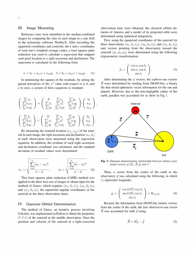
After determining the ρ vectors, the earth-to-sun vectors~R were determined by reading from DE405.bin, a binaryfile that stored ephemeris vector information for the sun andplanets. However, due to the non-negligible radius of theearth, parallax was accounted for as show in Fig 1.

Fig. 1: Diagram demonstrating relationship between relative posi-tional vectors ~ρ, ~RE , ~R,~g, and ~r.

Then, a vector from the center of the earth to theobservatory ~g was calculated using the following, in whichβi represents longitude:

gi =

cosLSTi cosβisinLSTi cosβi

sinβi

×Rearth. (4)

Because the information from DE405.bin returns vectorsfrom the center of the earth, the true observer-to-sun vector~R was accounted for with ~g using:

~R = ~RE − ~g (5)

3

After this parallax correction was completed for each ~R,each observation time was converted into modified days:

τ = k(t− t2). (6)

~r(τ) was then written as a Taylor series about τ2:

~r(τ) = a0 + a1 ~r2 + a2 ~r2 + a3 ~r2 + ... (7)

Due to the gravitational relation 11 the above Taylorseries for ~r(τ) can be simplified to terms containing onlyscalar multiples of ~r and ~r:

~r(τ) = f ~r2 + g ~r2, (8)

~r =−µ~rr3

. (9)

Considering only the fourth-order or lower terms of theabove Taylor series, f and g series were defined as:

f = [1− 1

2r03τ2 +

(~r0 ~r0)

2r05τ3 + ...], (10)

g = [τ − 1

6r03τ3 +

(~r0 ~r0)

4r05τ4 + ...]. (11)

Because the Taylor expansion of ~r was centered aboutτ2, the position vectors ~r1 and ~r3 were approximated byplugging τ1 and τ3 into the f and g series and eliminating~r2:

g3 ~r1 − g1 ~r3 = (f1g3 − f3g1)~r2. (12)

Using the vector triangle (see Figure 1) and a substi-tution for values of f1, f3, g1, and g3, constants useful indetermining ρ were calculated:

a1 =g3

f1g3 − f3g1, a2 = −1, a3 =

−g1f1g3 − f3g1

. (13)

The below equation follows from the vector triangle:

a1ρ1ρ1 − a2ρ2ρ2 + a3ρ3ρ3 = a1 ~R1 + a2 ~R2 + a3 ~R3. (14)

From here, through elimination of vectors through crossand dot products, (ρ1, ρ2, ρ3) can be solved for in thefollowing manner:

a1(R1 × ρ2) · ρ3 + a2( ~R2 × ρ2) · ρ3 + a3( ~R3 × ρ2) · ρ3a1(ρ1 × ρ2) · ρ3

,

(15)

a1(ρ1 ×R1) · ρ3 + a2(ρ1 ×R2) · ρ3 + a3(ρ1 ×R3) · ρ3a2(ρ1 × ρ2) · ρ3

,

(16)

a1(ρ2 ×R1) · ρ3 + a2(ρ2 ×R2) · ρ3 + a3(ρ2 ×R3) · ρ3a3(ρ1 × ρ2) · ρ3

.

(17)However, because the speed of light is finite, the true

time of observation of the asteroid was modified by thetime of light travel: ρ/c. So at each iteration, the new timecorrection with each new ρ was subtracted from the initiallyreported times. Once ρi and ρi have been calculated, ri canbe found using the following equation:

~r = ρρ− ~R (18)

However, since ~ri is needed to calculate ~ri, an initial guesswas needed before iterations start. For near-earth asteroids,a reasonable initial estimate is about 1.4 AU. Thus, finalvalues for ri were reached when the iterations above are rununtil ~rn and ~rn+1 differed by less than a threshold, suchas 10−15 AU. When the values converged, final ~ri and ρivalues were determined, and the velocity ~r was determinedas follows:

~r =f3

(g1f3 − g3f1)~r1 −

f1(g1f3 − g3f1)

~r3 (19)

Thus, with ~r2, ~r2, and a speed of light corrected t2determined, the vector state of the asteroid (~r2, ~r2, t2) canbe used to generate orbital elements.

V. Classical Orbital ElementsAfter the equatorial vector states have been determined

through the Method of Gauss, they were rotated to theecliptic plane through a rotation by −ε, the obliquity of theecliptic, along the x-axis. From there, the classical orbitalelements can be found as follows:

The semi-major axis can be found using the Vis-VivaEquation.

1

a=

2

|~r|− |~r|

2

µ(20)

4

Finds the eccentricity vector using the angular momentum,velocity, and radial vectors, which always points towardsthe perihelion.

~e = ~r × ~h− ~r

|~r|(21)

Inclination is the angle between the ecliptic plane an theorbital plane and is also equal to the angle between theangular momentum vector and the z axis.

i = cos-1(hz

|~h|) (22)

~N points towards the ascending node, and its directioncan be found by taking ~h× ~z.

~N =~z × ~h|~z × ~h|

(23)

Because x points to the vernal equinox, the longitude ofascending node can be found with ~N · ~x.

Ω =Nx

| ~N |(24)

Because ~N points to the ascending node and ~e pointstowards the perihelion, the angle between them can be foundwith the dot product.

ω = cos-1(~N · ~e

|~e| × | ~N |) (25)

Finally, by undoing the angle rotations of −Ω, −ω, and−i, the vectors can be transformed from ecliptic to orbitalcoordinates. Then, after finding the mean and accentricanomolies, the time of perihelion T was found:

T = t2 −M

k

√a3

µ(26)

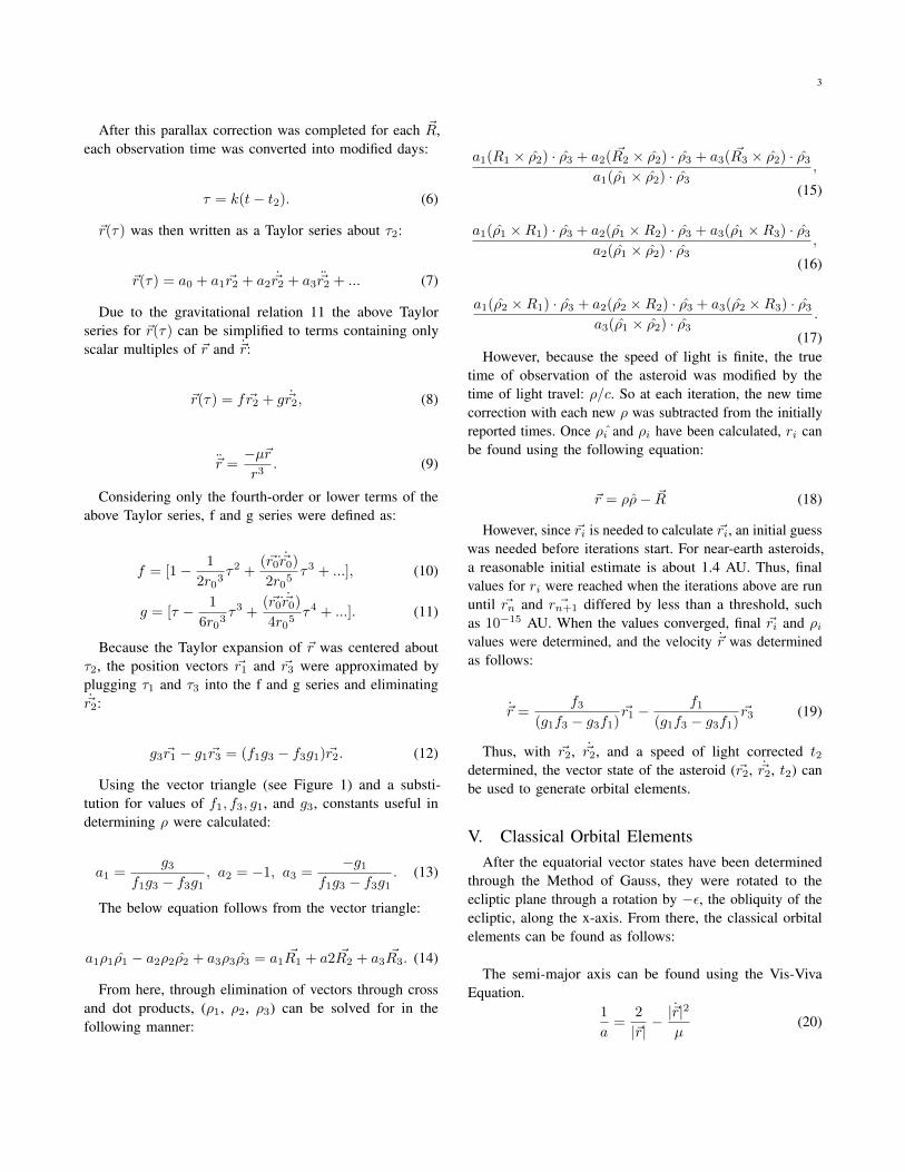
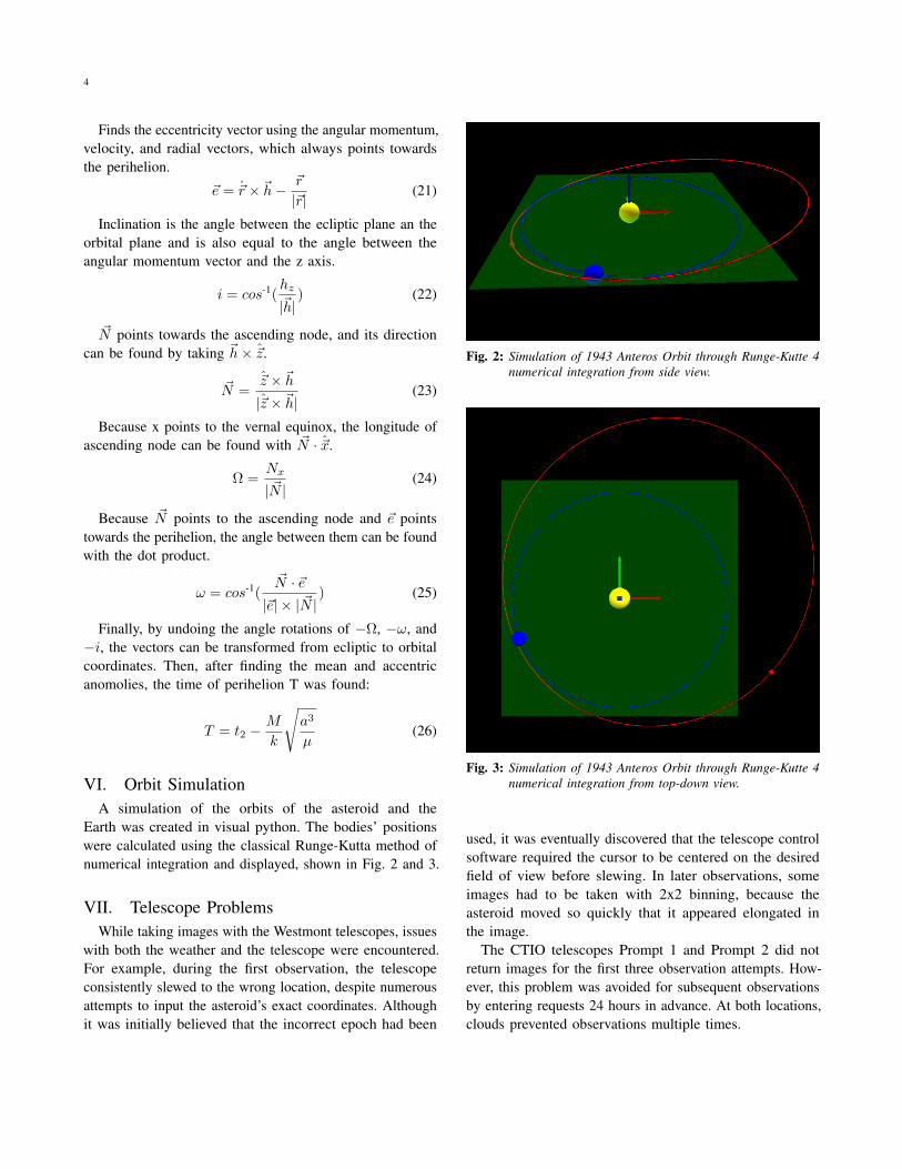
VI. Orbit SimulationA simulation of the orbits of the asteroid and the

Earth was created in visual python. The bodies’ positionswere calculated using the classical Runge-Kutta method ofnumerical integration and displayed, shown in Fig. 2 and 3.

VII. Telescope ProblemsWhile taking images with the Westmont telescopes, issues

with both the weather and the telescope were encountered.For example, during the first observation, the telescopeconsistently slewed to the wrong location, despite numerousattempts to input the asteroid’s exact coordinates. Althoughit was initially believed that the incorrect epoch had been

Fig. 2: Simulation of 1943 Anteros Orbit through Runge-Kutte 4numerical integration from side view.

Fig. 3: Simulation of 1943 Anteros Orbit through Runge-Kutte 4numerical integration from top-down view.

used, it was eventually discovered that the telescope controlsoftware required the cursor to be centered on the desiredfield of view before slewing. In later observations, someimages had to be taken with 2x2 binning, because theasteroid moved so quickly that it appeared elongated inthe image.

The CTIO telescopes Prompt 1 and Prompt 2 did notreturn images for the first three observation attempts. How-ever, this problem was avoided for subsequent observationsby entering requests 24 hours in advance. At both locations,clouds prevented observations multiple times.

5

III. RESULTS

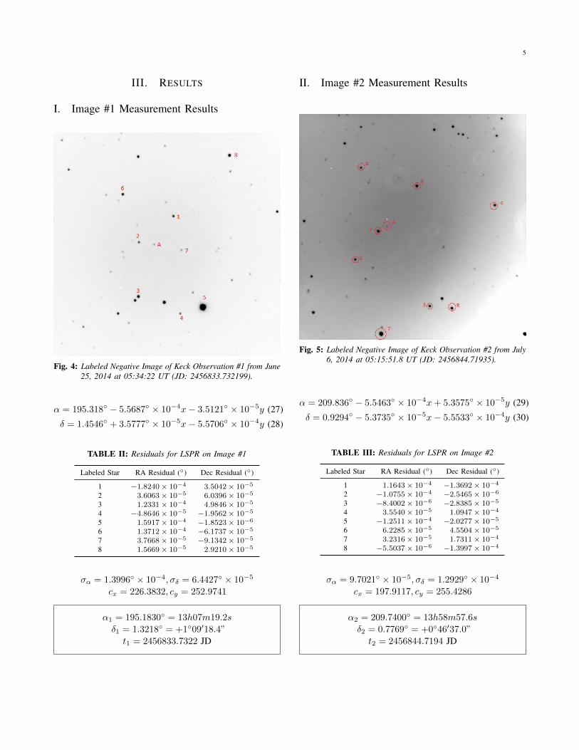
I. Image #1 Measurement Results

Fig. 4: Labeled Negative Image of Keck Observation #1 from June25, 2014 at 05:34:22 UT (JD: 2456833.732199).

α = 195.318 − 5.5687 × 10−4x− 3.5121 × 10−5y (27)

δ = 1.4546 + 3.5777 × 10−5x− 5.5706 × 10−4y (28)

TABLE II: Residuals for LSPR on Image #1

Labeled Star RA Residual () Dec Residual ()

1 −1.8240× 10−4 3.5042× 10−5

2 3.6063× 10−5 6.0396× 10−5

3 1.2331× 10−4 4.9846× 10−5

4 −4.8646× 10−5 −1.9562× 10−5

5 1.5917× 10−4 −1.8523× 10−6

6 1.3712× 10−4 −6.1737× 10−5

7 3.7668× 10−5 −9.1342× 10−5

8 1.5669× 10−5 2.9210× 10−5

σα = 1.3996 × 10−4, σδ = 6.4427 × 10−5

cx = 226.3832, cy = 252.9741

α1 = 195.1830 = 13h07m19.2s

δ1 = 1.3218 = +109′18.4”

t1 = 2456833.7322 JD

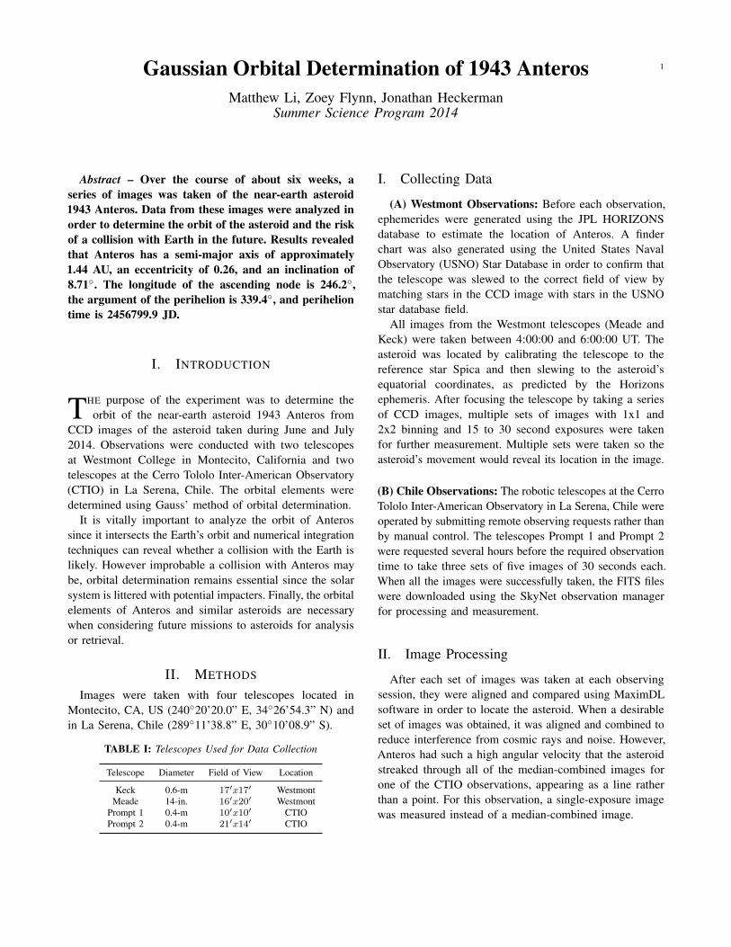
II. Image #2 Measurement Results

Fig. 5: Labeled Negative Image of Keck Observation #2 from July6, 2014 at 05:15:51.8 UT (JD: 2456844.71935).

α = 209.836 − 5.5463 × 10−4x+ 5.3575 × 10−5y (29)

δ = 0.9294 − 5.3735 × 10−5x− 5.5533 × 10−4y (30)

TABLE III: Residuals for LSPR on Image #2


1 1.1643× 10−4 −1.3692× 10−4

2 −1.0755× 10−4 −2.5465× 10−6

3 −8.4002× 10−6 −2.8385× 10−5

4 3.5540× 10−5 1.0947× 10−4

5 −1.2511× 10−4 −2.0277× 10−5

6 6.2285× 10−5 4.5504× 10−5

7 3.2316× 10−5 1.7311× 10−4

8 −5.5037× 10−6 −1.3997× 10−4

σα = 9.7021 × 10−5, σδ = 1.2929 × 10−4

cx = 197.9117, cy = 255.4286

α2 = 209.7400 = 13h58m57.6s

δ2 = 0.7769 = +046′37.0”

t2 = 2456844.7194 JD

6

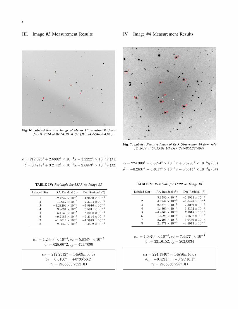
III. Image #3 Measurement Results

Fig. 6: Labeled Negative Image of Meade Observation #3 fromJuly 8, 2014 at 04:54:19.34 UT (JD: 2456846.704390).

α = 212.096 + 2.6892 × 10−4x− 3.2222 × 10−5y (31)

δ = 0.4742 + 3.2112 × 10−5x+ 2.6853 × 10−4y (32)

TABLE IV: Residuals for LSPR on Image #3


1 −2.4742× 10−5 −1.9550× 10−5

2 1.9052× 10−4 7.3304× 10−6

3 −1.28204× 10−4 −7.9916× 10−6

4 9.9691× 10−5 6.5911× 10−5

5 −5.1130× 10−5 −8.8008× 10−5

6 −9.7183× 10−5 −6.2144× 10−6

7 −1.2014× 10−5 −1.5979× 10−5

8 2.3059× 10−5 6.4502× 10−5

σα = 1.2330 × 10−4, σδ = 5.8385 × 10−5

cx = 628.6672, cy = 451.7090

α3 = 212.2512 = 14h09m00.3s

δ3 = 0.6156 = +036′56.2”

t3 = 2456833.7322 JD

IV. Image #4 Measurement Results

Fig. 7: Labeled Negative Image of Keck Observation #4 from July18, 2014 at 05:15:01 UT (JD: 2456856.725694).

α = 224.303 − 5.5524 × 10−4x+ 5.3798 × 10−5y (33)

δ = −0.2637 − 5.4017 × 10−5x− 5.5514 × 10−4y (34)

TABLE V: Residuals for LSPR on Image #4


1 5.6580× 10−6 −2.4022× 10−5

2 4.8742× 10−5 −1.0428× 10−4

3 2.5375× 10−5 7.3069× 10−5

4 −1.4309× 10−4 1.3392× 10−5

5 −4.4360× 10−5 7.1018× 10−5

6 1.6520× 10−4 −3.7637× 10−5

7 −8.2295× 10−5 5.0430× 10−5

8 2.4771× 10−5 −4.1973× 10−5

σα = 1.0970 × 10−4, σδ = 7.4477 × 10−4

cx = 221.6152, cy = 262.0034

α4 = 224.1940 = 14h56m46.6s

δ4 = −0.4211 = −025′16.1”

t4 = 2456856.7257 JD

7

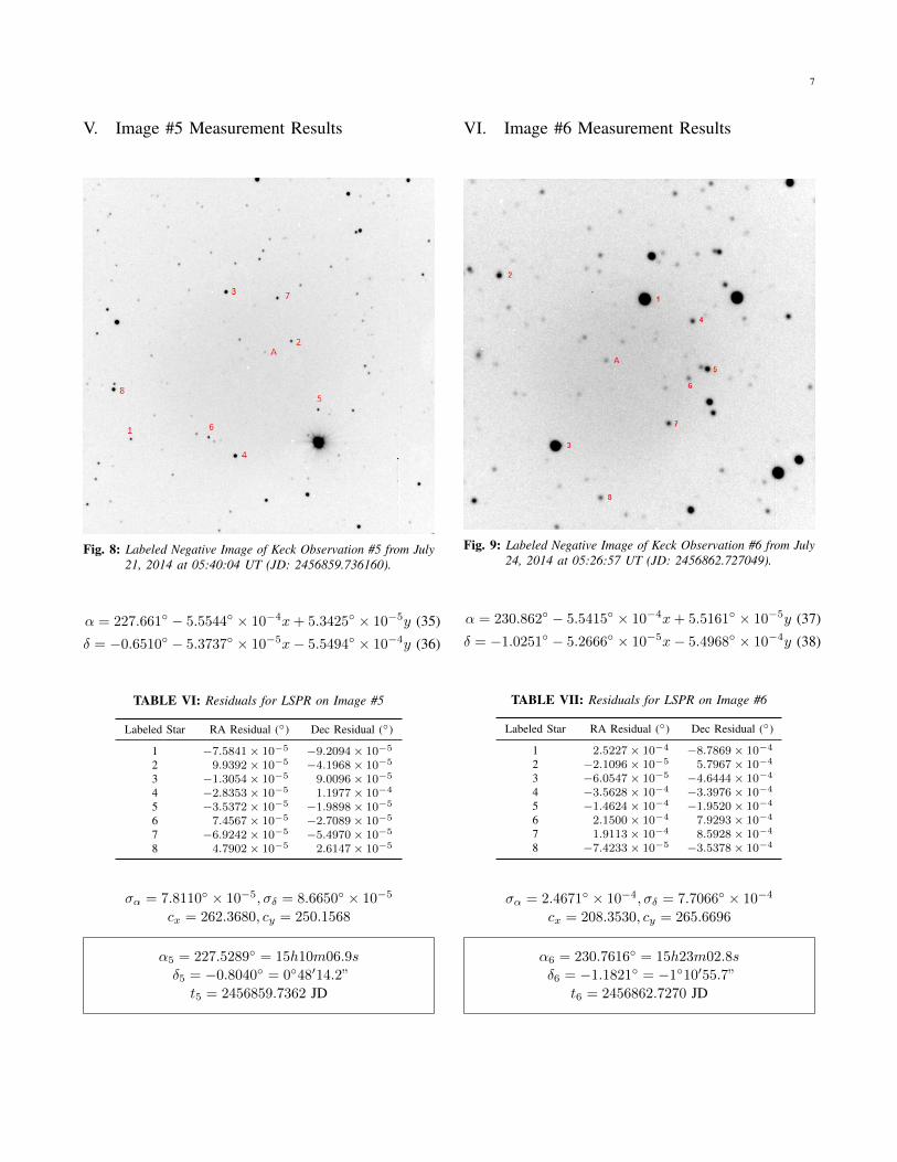
V. Image #5 Measurement Results


α = 227.661 − 5.5544 × 10−4x+ 5.3425 × 10−5y (35)

δ = −0.6510 − 5.3737 × 10−5x− 5.5494 × 10−4y (36)

TABLE VI: Residuals for LSPR on Image #5


1 −7.5841× 10−5 −9.2094× 10−5

2 9.9392× 10−5 −4.1968× 10−5

3 −1.3054× 10−5 9.0096× 10−5

4 −2.8353× 10−5 1.1977× 10−4

5 −3.5372× 10−5 −1.9898× 10−5

6 7.4567× 10−5 −2.7089× 10−5

7 −6.9242× 10−5 −5.4970× 10−5

8 4.7902× 10−5 2.6147× 10−5

σα = 7.8110 × 10−5, σδ = 8.6650 × 10−5

cx = 262.3680, cy = 250.1568

α5 = 227.5289 = 15h10m06.9s

δ5 = −0.8040 = 048′14.2”

t5 = 2456859.7362 JD

VI. Image #6 Measurement Results


α = 230.862 − 5.5415 × 10−4x+ 5.5161 × 10−5y (37)

δ = −1.0251 − 5.2666 × 10−5x− 5.4968 × 10−4y (38)

TABLE VII: Residuals for LSPR on Image #6


1 2.5227× 10−4 −8.7869× 10−4

2 −2.1096× 10−5 5.7967× 10−4

3 −6.0547× 10−5 −4.6444× 10−4

4 −3.5628× 10−4 −3.3976× 10−4

5 −1.4624× 10−4 −1.9520× 10−4

6 2.1500× 10−4 7.9293× 10−4

7 1.9113× 10−4 8.5928× 10−4

8 −7.4233× 10−5 −3.5378× 10−4

σα = 2.4671 × 10−4, σδ = 7.7066 × 10−4

cx = 208.3530, cy = 265.6696

α6 = 230.7616 = 15h23m02.8s

δ6 = −1.1821 = −110′55.7”

t6 = 2456862.7270 JD

8

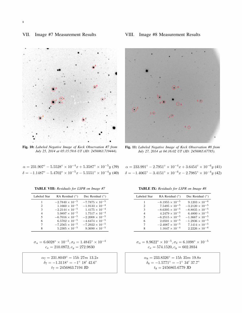
VII. Image #7 Measurement Results

Fig. 10: Labeled Negative Image of Keck Observation #7 fromJuly 25, 2014 at 05:15:59.6 UT (JD: 2456863.719444).

α = 231.907 − 5.5528 × 10−4x+ 5.3587 × 10−5y (39)

δ = −1.1487 − 5.4702 × 10−5x− 5.5551 × 10−4y (40)

TABLE VIII: Residuals for LSPR on Image #7


1 −2.7840× 10−5 −7.7875× 10−5

2 1.1660× 10−5 −1.9133× 10−4

3 −2.2144× 10−5 1.4175× 10−4

4 5.9897× 10−5 1.7517× 10−4

5 −6.7016× 10−5 −2.2008× 10−5

6 6.5702× 10−5 −4.6474× 10−5

7 −7.2565× 10−5 −7.2922× 10−5

8 5.2305× 10−5 9.3690× 10−5

σα = 6.6028 × 10−5, σδ = 1.4845 × 10−4

cx = 210.0972, cy = 272.9830

α7 = 231.8049 = 15h 27m 13.2s

δ7 = −1.3118 = −1 18′ 42.6”

t7 = 2456863.7194 JD

VIII. Image #8 Measurement Results

Fig. 11: Labeled Negative Image of Keck Observation #8 fromJuly 27, 2014 at 04:16:02 UT (JD: 2456865.67785).

α = 233.991 − 2.7951 × 10−4x+ 3.6454 × 10−6y (41)

δ = −1.4065 − 3.4151 × 10−6x− 2.7985 × 10−4y (42)

TABLE IX: Residuals for LSPR on Image #8


1 −8.1955× 10−5 9.1203× 10−6

2 7.5495× 10−5 −3.2120× 10−5

3 −8.6395× 10−5 −8.8835× 10−5

4 4.2479× 10−5 6.4800× 10−5

5 −6.2515× 10−5 −1.3667× 10−5

6 2.0501× 10−5 −1.2936× 10−5

7 −2.4087× 10−5 7.1414× 10−5

8 1.1647× 10−4 2.2226× 10−6

σα = 8.9622 × 10−5, σδ = 6.1098 × 10−5

cx = 574.1520, cy = 602.3934

α8 = 233.8326 = 15h 35m 19.8s

δ8 = −1.5771 = −1 34′ 37.7”

t8 = 2456865.6779 JD

9

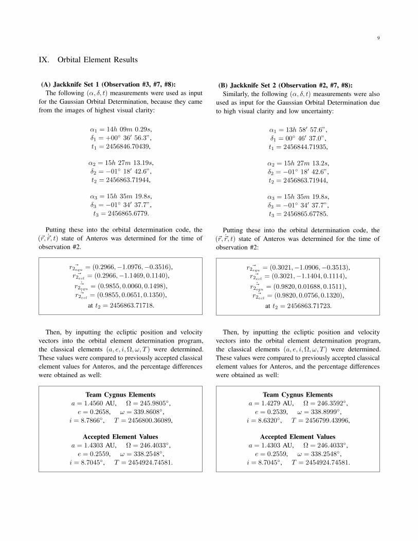
IX. Orbital Element Results

(A) Jackknife Set 1 (Observation #3, #7, #8):The following (α, δ, t) measurements were used as input

for the Gaussian Orbital Determination, because they camefrom the images of highest visual clarity:

α1 = 14h 09m 0.29s,δ1 = +00 36′ 56.3”,t1 = 2456846.70439,

α2 = 15h 27m 13.19s,δ2 = −01 18′ 42.6”,t2 = 2456863.71944,

α3 = 15h 35m 19.8s,δ3 = −01 34′ 37.7”,t3 = 2456865.6779.

Putting these into the orbital determination code, the(~r, ~r, t) state of Anteros was determined for the time ofobservation #2.

~r2equ = (0.2966,−1.0976,−0.3516),~r2ecl = (0.2966,−1.1469, 0.1140),

~r2equ = (0.9855, 0.0060, 0.1498),~r2ecl = (0.9855, 0.0651, 0.1350),

at t2 = 2456863.71718.

Then, by inputting the ecliptic position and velocityvectors into the orbital element determination program,the classical elements (a, e, i,Ω, ω, T ) were determined.These values were compared to previously accepted classicalelement values for Anteros, and the percentage differenceswere obtained as well:

Team Cygnus Elementsa = 1.4560 AU, Ω = 245.9805,e = 0.2658, ω = 339.8608,

i = 8.7866, T = 2456800.36089,

Accepted Element Valuesa = 1.4303 AU, Ω = 246.4033,e = 0.2559, ω = 338.2548,

i = 8.7045, T = 2454924.74581.

(B) Jackknife Set 2 (Observation #2, #7, #8):Similarly, the following (α, δ, t) measurements were also

used as input for the Gaussian Orbital Determination dueto high visual clarity and low uncertainty:

α1 = 13h 58′ 57.6”,δ1 = 00 46′ 37.0”,t1 = 2456844.71935,

α2 = 15h 27m 13.2s,δ2 = −01 18′ 42.6”,t2 = 2456863.71944,

α3 = 15h 35m 19.8s,δ3 = −01 34′ 37.7”,t3 = 2456865.67785.

Putting these into the orbital determination code, the(~r, ~r, t) state of Anteros was determined for the time ofobservation #2:

~r2equ = (0.3021,−1.0906,−0.3513),~r2ecl = (0.3021,−1.1404, 0.1114),

~r2equ = (0.9820, 0.01688, 0.1511),~r2ecl = (0.9820, 0.0756, 0.1320),

at t2 = 2456863.71723.

Then, by inputting the ecliptic position and velocityvectors into the orbital element determination program,the classical elements (a, e, i,Ω, ω, T ) were determined.These values were compared to previously accepted classicalelement values for Anteros, and the percentage differenceswere obtained as well:

Team Cygnus Elementsa = 1.4279 AU, Ω = 246.3592,e = 0.2539, ω = 338.8999,

i = 8.6320, T = 2456799.43996,


i = 8.7045, T = 2454924.74581.

10

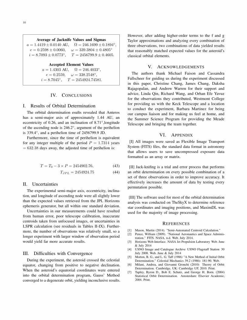
Average of Jacknife Values and Sigmasa = 1.4419± 0.0140 AU, Ω = 246.1699± 0.1894,e = 0.2598± 0.0060, ω = 339.3804± 0.4805

i = 8.7093± 0.0773, T = 2456799.9± 0.4605.


i = 8.7045, T = 2454924.74581.

IV. CONCLUSIONS

I. Results of Orbital DeterminationThe orbital determination esults revealed that Anteros

has a semi-major axis of approximately 1.44 AU, aneccentricity of 0.26, and an inclination of 8.71,longitudeof the ascending node is 246.2, argument of the perihelionis 339.4, and a perihelion time of 2456799.9 JD.

Furthermore, since the time of perihelion is equivalentfor any integer multiple of the period P = 1.7314 years= 632.38 days away, the adjusted time of perihelion is:

T = T0 − 3× P = 2454902.76, (43)

TJPL = 2454924.75 (44)

II. UncertaintiesThe experimental semi-major axis, eccentricity, inclina-

tion, and longitude of ascending node were all slightly lowerthan the expected values retrieved from the JPL Horizonsephemeris generator, but all within one standard deviation.

Uncertainties in our measurements could have resultedfrom human error, poor telescope calibration, inaccuratecentroids taken from unfocused images, or uncertainties inLSPR calculation (see residuals in Tables II-IX). Further-more, the number of observations was relatively small, so alonger experiment with larger window of observation periodwould yield far more accurate results.

III. Difficulties with ConvergenceDuring the experiment, the asteroid crossed the celestial

equator, changing from positive to negative declination.When the asteroid’s equatorial coordinates were enteredinto the orbital determination program, Gauss’ Methodconverged to a degenerate orbit, yielding inconclusive results.

However, after adding higher-order terms to the f and gTaylor approximations and analyzing every combination ofthree observations, two combinations of data yielded resultsthat reasonably matched expected values for the asteroid’sclassical orbital elements.

V. ACKNOWLEDGEMENTS

The authors thank Michael Faison and CassandraFallscheer for guiding us during the experiment discussedin this paper, Christine Chang, James Chang, DakshaRajagopalan, and Andrew Warren for their support andadvice, Linda Qin, Richard Wang, and Orhan Efe Yavuzfor the observations they contributed, Westmont Collegefor providing us with the Keck Telescope and a locationto conduct the experiment, Barbara Martinez for beingour campus liaison and for making us feel at home, andthe Summer Science Program for providing the MeadeTelescope and bringing the team together.

VI. APPENDIX

[I] All images were saved as Flexible Image TransportSystem (FITS) files, the standard data format in astronomythat allows users to save uncompressed exposure dataformatted as an array or matrix.

[II] Jack-knifing is a trial and error process that performsan orbit determination on every possible combination of aset of three observations in order to improve accuracy. Iteffectively increases the amount of data by testing everypermutation possible.

[III] The software used for most of the orbital determinationanalysis was conducted on TheSkyX to determine referencestar coordinates and imaging positions, and MaximDL wasused for the majority of image processing.

REFERENCES

[1] Mason, Martin (2014). "Semi-Automated Centroid Calculation."[2] Pence, William (2009). "National Aeronautics and Space Adminis-

tration." FITS. NASA, n.d. Web. July 2014.[3] Horizons Web-Interface. NASA Jet Propulsion Laboratory Web. June

& July 2014[4] USNO Image and Catalogue Archive USNO Flagstaff Station 30

July 2008. Web. June & July 2014[5] Morton, B. G., and L. G. Taff (1986) "A New Method of Initial Orbit

Determination." Celestial Mechanics 39.2 (1986): 181-90. Web.[6] Milani, Andrea, and Giovanni Gronchi (2010) Theory of Orbit

Determination. Cambridge, UK: Cambridge UP, 2010. Print.[7] Tapley, Byron D., Bob E. Schutz, and George H. Born. (2004)

Statistical Orbit Determination. Amsterdam: Elsevier Academic,2004. Print.