Embed Size (px)
Citation preview

– p.1

Thanks
Collaborators:Felix AbramowichYoav BenjaminiDavid DonohoNoureddine El KarouiPeter ForresterGerard KerkyacharianDebashis PaulDominique PicardBernard Silverman
Presentation help: B. Narasimhan, N. El Karoui, J-MCorcuera
Grant Support: NIH, NSF, ARC (via P. Hall)
– p.2

Abraham Wald
– p.3

Three Talks
1. Function Estimation & Classical Normal Theory• Xn ∼ Np(n)(θn, I) p(n) ↗ with n (MVN)
2. The Threshold Selection Problem• In (MVN) with, say, θi = XiI{|Xi| > t}• How to select t = t(X)“reliably”?
3. Large Covariance Matrices
• Xn ∼ Np(n)(I ⊗ Σp(n)); especially Xn =
[Yn
Zn
]
• spectral properties of n−1XnXTn
• PCA, CCA, MANOVA
– p.4
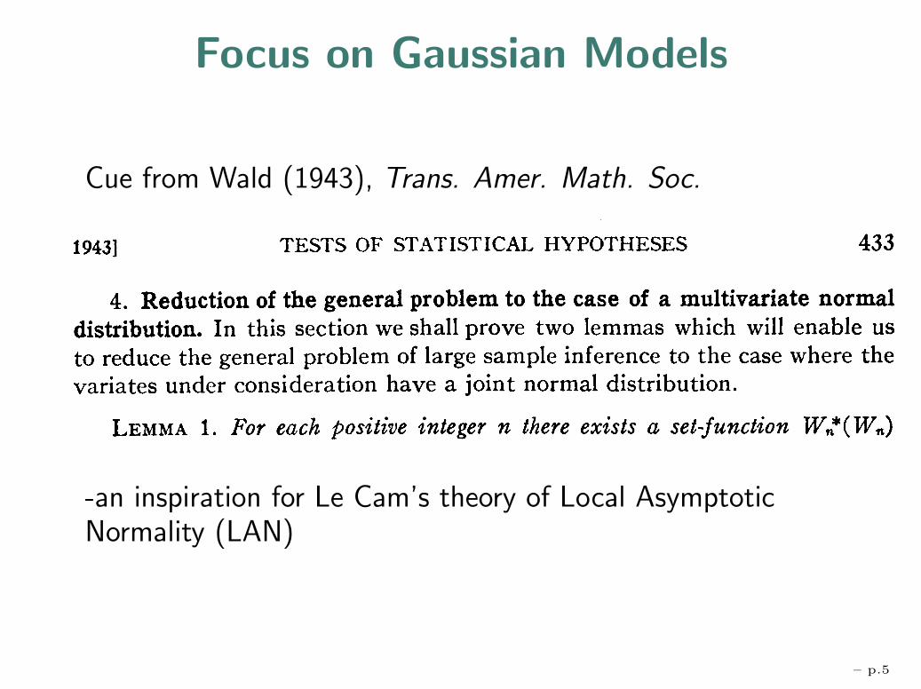
Focus on Gaussian Models
Cue from Wald (1943), Trans. Amer. Math. Soc.
-an inspiration for Le Cam’s theory of Local AsymptoticNormality (LAN)
– p.5

Focus on Gaussian Models, ctd.
• “Growing models”: p � n or p� n is now commonplace(classification, genomics..)
• Reality check:
“But, no real data is Gaussian...”
Yes (in many fields), and yet,
consider the power of fable and fairy tale...
– p.6
1. Function Estimation and ClassicalNormal Theory
Theme:
Gaussian White Noise model & multiresolution point of view
allow classical parametric theory of Nd(θ, I)
to be exploited in nonparametric function estimation
Reference: book manuscript in (non-)progress:
Function Estimation and Gaussian Sequence Models
www-stat.stanford.edu/~imj
– p.7

Agenda
• Classical Parametric Ideas
• Nonparametric Estimation and
Growing Gaussian Models
• I. Kernel Estimation and James-Stein Shrinkage
• II. Thresholding and Sparsity
• III. Bernstein-von Mises phenomenon
– p.8

Classical Ideas
a) Multinormal shift model
X1, . . . , Xn data from Pη(dx) = fη(x)µ(dx), η ∈ H ⊂ Rd.
Let I0 = Fisher information matrix at η0.
Local asymptotic Gaussian approximation:
{Pnη0+θ/
√n , θ ∈ R
d} ≈ {Nd(θ, I−10 ) , θ ∈ R
d}
– p.9

Classical Ideas, ctd
b) ANOVA, Projections and Model Selection
Yn×1
= X βn×d d×1
+ σε
Submodels: X = [X0 X1] → projections PX0.
Canonical form: y = θ + σz.
Projections: (P0y)i =
{yi i ∈ I0
0 o/w
MSE: E‖P0y − θ‖2 =∑
i∈I0σ2 +
∑i/∈I0
θ2i
– p.10

Classical Ideas, ctd
c) Minimax estimation of θ
infθ
supθ∈Rd
Eθ‖θ(y) − θ‖2 = dσ2
attained by MLE θMLE(y) = y.
d) James-Stein estimate
θJS(y) =(1 − d− 2
‖y‖2
)y
dominates MLE if d ≥ 3.
– p.11
Classical Ideas, ctd
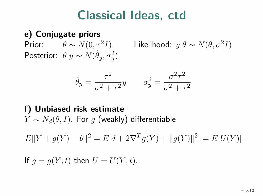
e) Conjugate priorsPrior: θ ∼ N(0, τ2I), Likelihood: y|θ ∼ N(θ, σ2I)
Posterior: θ|y ∼ N(θy, σ2y)
θy =τ2
σ2 + τ2y σ2
y =σ2τ2
σ2 + τ2
f) Unbiased risk estimateY ∼ Nd(θ, I). For g (weakly) differentiable
E‖Y + g(Y ) − θ‖2 = E[d+ 2∇T g(Y ) + ‖g(Y )‖2] = E[U(Y )]
If g = g(Y ; t) then U = U(Y ; t).
– p.12

Agenda
• Classical Parametric Ideas
• Nonparametric Estimation and
Growing Gaussian Models
• I. Kernel Estimation and James-Stein Shrinkage
• II. Thresholding and Sparsity
• III. Bernstein-von Mises phenomenon
– p.13
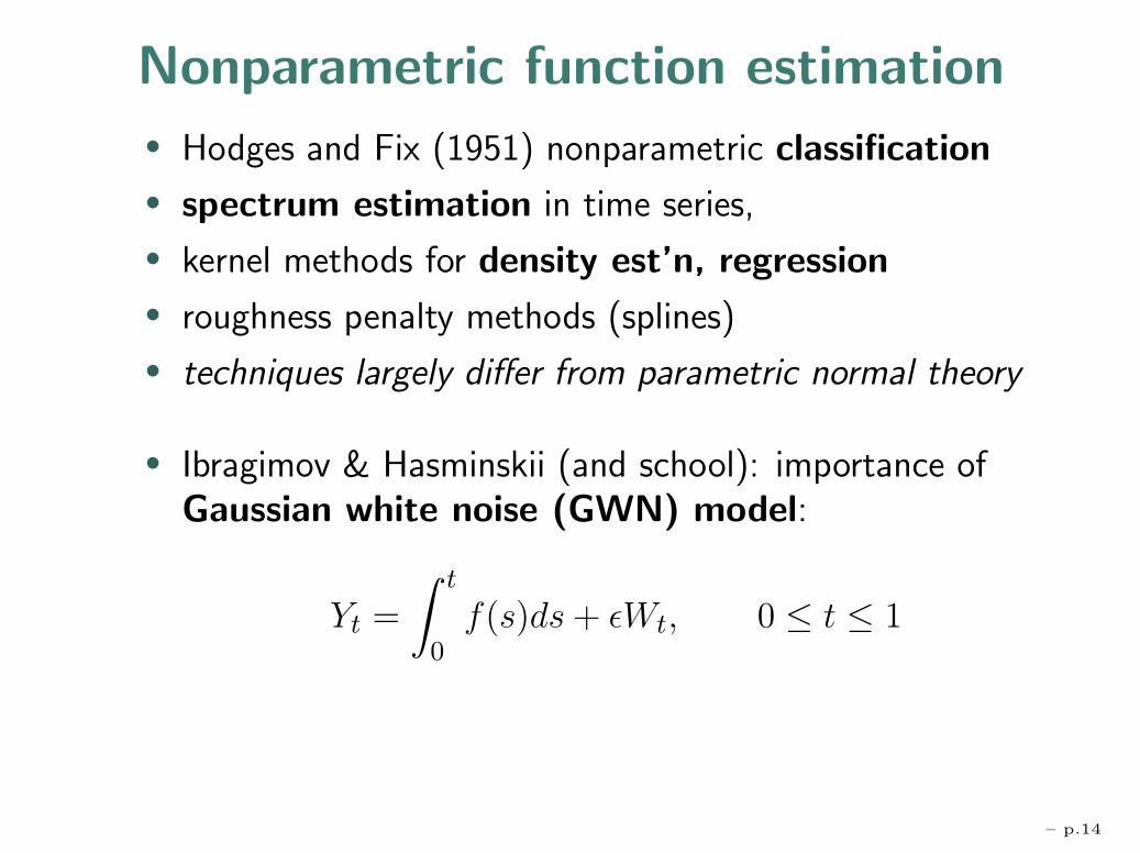
Nonparametric function estimation
• Hodges and Fix (1951) nonparametric classification
• spectrum estimation in time series,
• kernel methods for density est’n, regression
• roughness penalty methods (splines)
• techniques largely differ from parametric normal theory
• Ibragimov & Hasminskii (and school): importance ofGaussian white noise (GWN) model:
Yt =
∫ t
0f(s)ds+ εWt, 0 ≤ t ≤ 1
– p.14
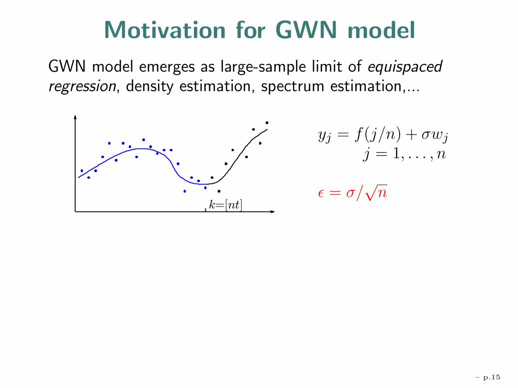
Motivation for GWN model
GWN model emerges as large-sample limit of equispacedregression, density estimation, spectrum estimation,...
yj = f(j/n) + σwj
j = 1, . . . , n
ε = σ/√n
– p.15
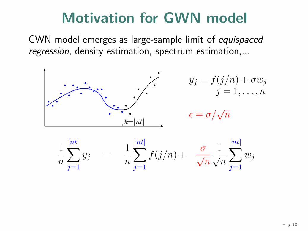
Motivation for GWN model
GWN model emerges as large-sample limit of equispacedregression, density estimation, spectrum estimation,...
yj = f(j/n) + σwj
j = 1, . . . , n
ε = σ/√n
1
n
[nt]∑j=1
yj =1
n
[nt]∑j=1
f(j/n) +σ√n
1√n
[nt]∑j=1
wj
– p.15

Motivation for GWN model
GWN model emerges as large-sample limit of equispacedregression, density estimation, spectrum estimation,...
yj = f(j/n) + σwj
j = 1, . . . , n
ε = σ/√n
1
n
[nt]∑j=1
yj =1
n
[nt]∑j=1
f(j/n) +σ√n
1√n
[nt]∑j=1
wj
Yt =
∫ t
0f(s)ds +
σ√n
· Wt
– p.15

Series form of WN Model
Yt =
∫ t
0f(s)ds+ εWt
For any orthonormal basis {ψλ, λ ∈ Λ} for L2[0, 1],∫ψλdYt =
∫ψλfdt+ ε
∫ψλdWt
⇒ yλ = θλ + εzλ, (zλ)i.i.d.∼ N(0, 1), λ ∈ Λ
Parseval relation implies∫(f − f)2 =
∑(θλ − θλ)2 = ‖θ − θ‖2, etc.
→ analysis of infinite sequences in 2(N)
– p.16
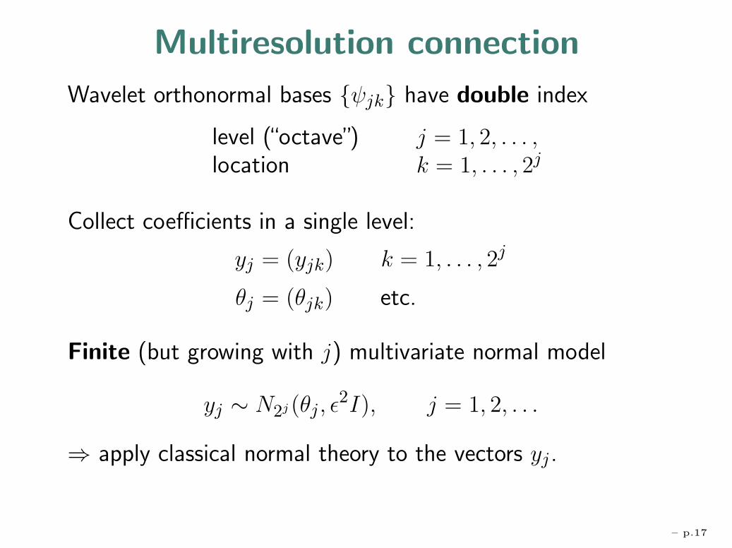
Multiresolution connection
Wavelet orthonormal bases {ψjk} have double index
level (“octave”) j = 1, 2, . . . ,location k = 1, . . . , 2j
Collect coefficients in a single level:
yj = (yjk) k = 1, . . . , 2j
θj = (θjk) etc.
Finite (but growing with j) multivariate normal model
yj ∼ N2j(θj , ε2I), j = 1, 2, . . .
⇒ apply classical normal theory to the vectors yj.
– p.17

0 0.1 0.2 0.3 0.4 0.5 0.6 0.7 0.8 0.9 10
2
4
6
8
10
12
14
16Some S8 Symmlets at various scales and locations
(4, 3)
(4, 8)
(4,11)
(6,12)
(6,26)
(6,34)
(6,42)
(7,51)
(7,77)
(7,101)
(8,31)
(8,81)
(8,102)
(8,166)
(8,202)
– p.18
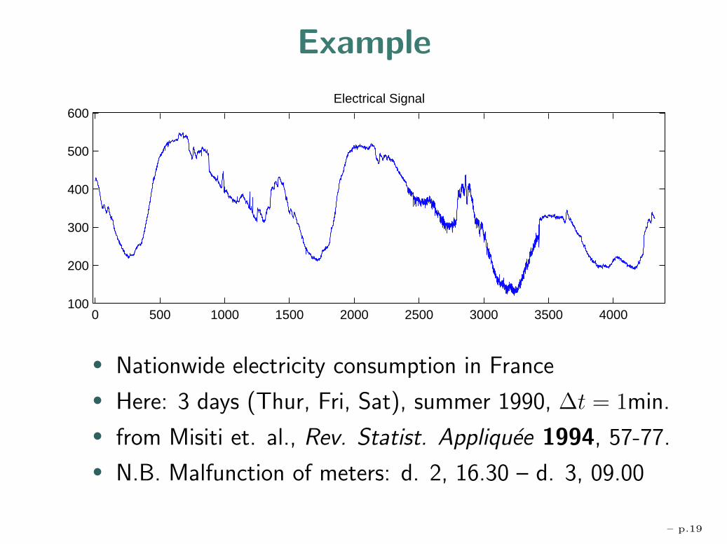
Example
0 500 1000 1500 2000 2500 3000 3500 4000100
200
300
400
500
600Electrical Signal
• Nationwide electricity consumption in France
• Here: 3 days (Thur, Fri, Sat), summer 1990, ∆t = 1min.
• from Misiti et. al., Rev. Statist. Appliquee 1994, 57-77.
• N.B. Malfunction of meters: d. 2, 16.30 – d. 3, 09.00
– p.19
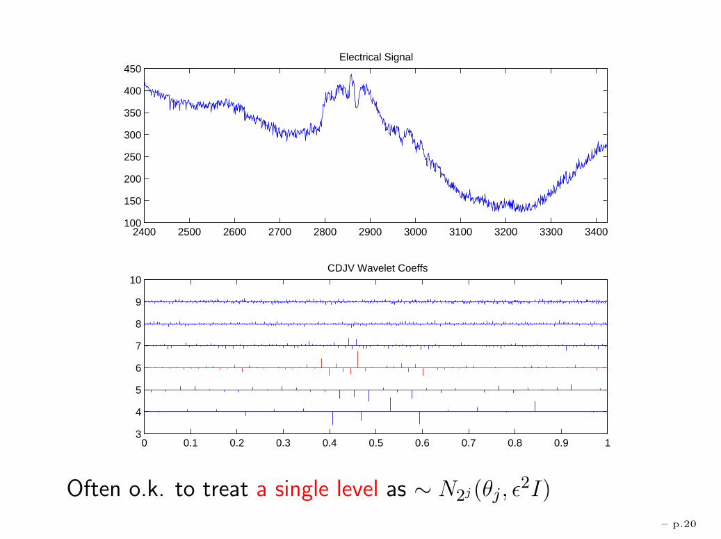
2400 2500 2600 2700 2800 2900 3000 3100 3200 3300 3400100
150
200
250
300
350
400
450Electrical Signal
0 0.1 0.2 0.3 0.4 0.5 0.6 0.7 0.8 0.9 13
4
5
6
7
8
9
10 CDJV Wavelet Coeffs
Often o.k. to treat a single level as ∼ N2j(θj , ε2I)
– p.20
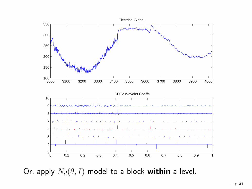
3000 3100 3200 3300 3400 3500 3600 3700 3800 3900 4000100
150
200
250
300
350Electrical Signal
0 0.1 0.2 0.3 0.4 0.5 0.6 0.7 0.8 0.9 13
4
5
6
7
8
9
10 CDJV Wavelet Coeffs
Or, apply Nd(θ, I) model to a block within a level.
– p.21

The Minimax principle
Given loss function L(a, θ), and risk
R(θ, θ) = EθL(θ, θ)
choose estimator θ so as to minimize the maximum risksupθ∈Θ
EθL(θ, θ).
• introduced into statistics by Wald
• L.J. Savage (1951):
“the only rule of comparable generality proposedsince [that of] Bayes’ was published in 1763”
• standard complaint: θ depends on Θ:• optimizing on the worst case may be irrelevant
– p.22
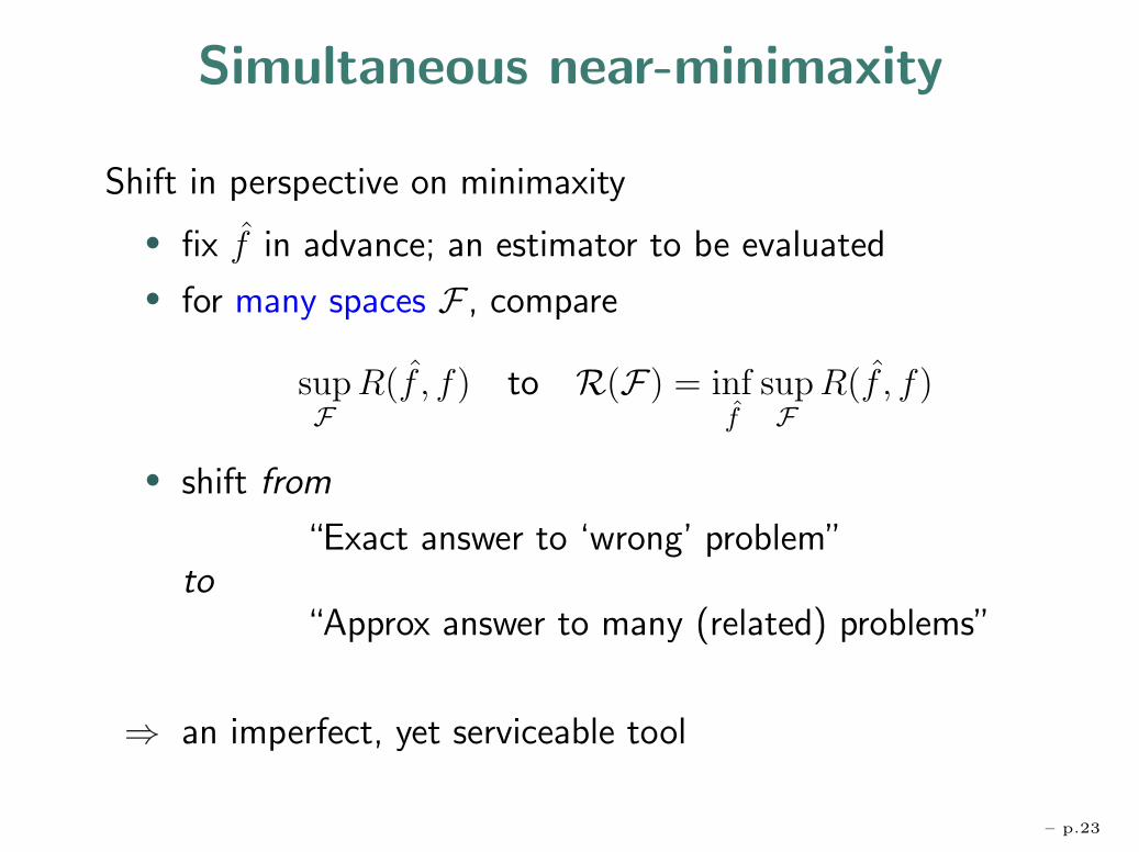
Simultaneous near-minimaxity
Shift in perspective on minimaxity
• fix f in advance; an estimator to be evaluated
• for many spaces F , compare
supFR(f , f) to R(F) = inf
fsupFR(f , f)
• shift from
“Exact answer to ‘wrong’ problem”to
“Approx answer to many (related) problems”
⇒ an imperfect, yet serviceable tool
– p.23

Agenda
• Classical Parametric Ideas
• Nonparametric Estimation and
Growing Gaussian Models
• I. Kernel Estimation and James-Stein Shrinkage
• II. Thresholding and Sparsity
• III. Bernstein-von Mises phenomenon
– p.24
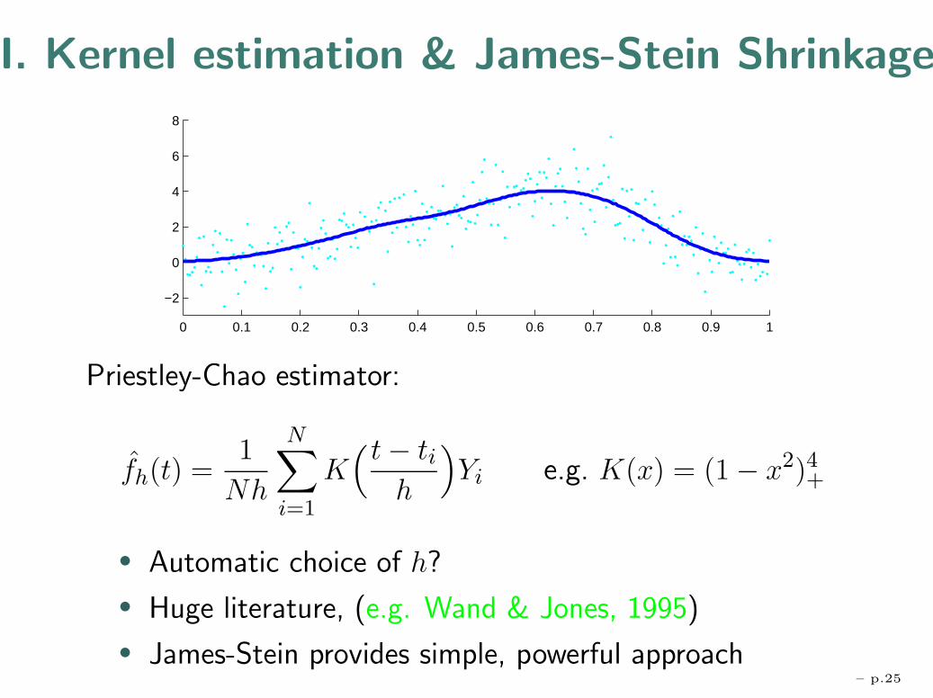
I. Kernel estimation & James-Stein Shrinkage
0 0.1 0.2 0.3 0.4 0.5 0.6 0.7 0.8 0.9 1
−2
0
2
4
6
8
Priestley-Chao estimator:
fh(t) =1
Nh
N∑i=1
K(t− ti
h
)Yi e.g. K(x) = (1 − x2)4+
• Automatic choice of h?
• Huge literature, (e.g. Wand & Jones, 1995)
• James-Stein provides simple, powerful approach– p.25

Fourier Form of Kernel Smoothing
Convolution → multiplication
Shrinkage factors
• sk(h) ∈ [0, 1]
• decrease with frequency
TFD
TFDi
)knirhs(
Flatten shrinkage in blocks:
θk = (1 − wj)yk k ∈ Bj
• How to choose wj?
ycneuqerf
– p.26

James-Stein Shrinkage
For y ∼ Nd(θ, I), and d ≥ 3
θJS+ =
(1 − d− 2 + η
|y|2)
+
y
Unbiased estimate of risk:
E‖θJS − θ‖2 = Eθ
{d− (d− 2)2 + η2
‖y‖2
}≤ d
– p.27
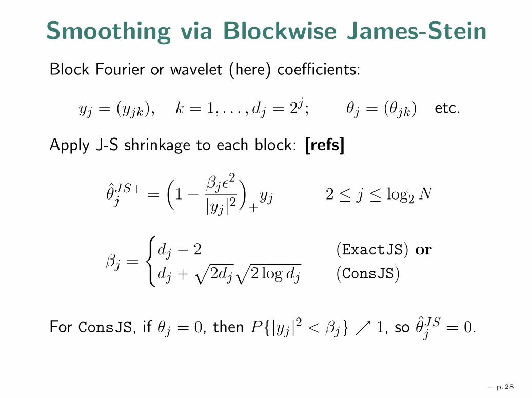
Smoothing via Blockwise James-Stein
Block Fourier or wavelet (here) coefficients:
yj = (yjk), k = 1, . . . , dj = 2j ; θj = (θjk) etc.
Apply J-S shrinkage to each block: [refs]
θJS+j =
(1 − βjε
2
|yj|2)
+yj 2 ≤ j ≤ log2N
βj =
{dj − 2 (ExactJS) or
dj +√
2dj
√2 log dj (ConsJS)
For ConsJS, if θj = 0, then P{|yj |2 < βj} ↗ 1, so θJSj = 0.
– p.28

Block James-Stein imitates Kernel
0 0.1 0.2 0.3 0.4 0.5 0.6 0.7 0.8 0.9 1
−2
0
2
4
6
8
0 0.1 0.2 0.3 0.4 0.5 0.6 0.7 0.8 0.9 1
−2
0
2
4
6
8
– p.29
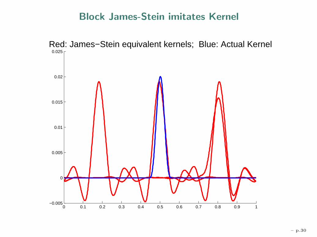
Block James-Stein imitates Kernel
0 0.1 0.2 0.3 0.4 0.5 0.6 0.7 0.8 0.9 1−0.005
0
0.005
0.01
0.015
0.02
0.025Red: James−Stein equivalent kernels; Blue: Actual Kernel
– p.30

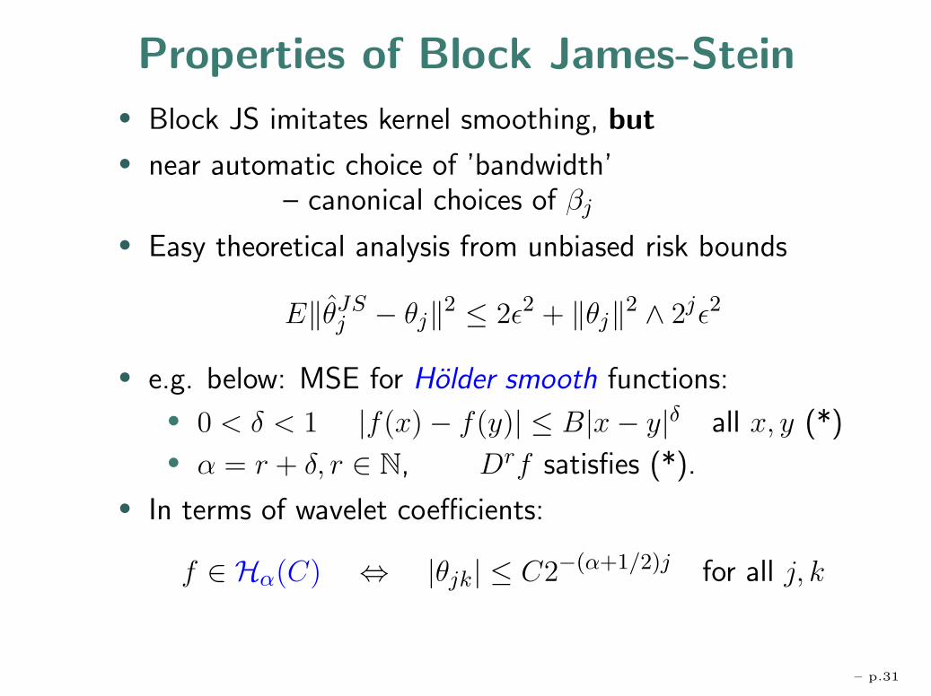
Properties of Block James-Stein• Block JS imitates kernel smoothing, but
• near automatic choice of ’bandwidth’– canonical choices of βj
• Easy theoretical analysis from unbiased risk bounds
E‖θJSj − θj‖2 ≤ 2ε2 + ‖θj‖2 ∧ 2jε2
– p.31
Properties of Block James-Stein• Block JS imitates kernel smoothing, but
• near automatic choice of ’bandwidth’– canonical choices of βj
• Easy theoretical analysis from unbiased risk bounds
E‖θJSj − θj‖2 ≤ 2ε2 + ‖θj‖2 ∧ 2jε2
• e.g. below: MSE for Holder smooth functions:• 0 < δ < 1 |f(x) − f(y)| ≤ B|x− y|δ all x, y (*)• α = r + δ, r ∈ N, Drf satisfies (*).
• In terms of wavelet coefficients:
f ∈ Hα(C) ⇔ |θjk| ≤ C2−(α+1/2)j for all j, k
– p.31

A single level determines MSE
From unbiased risk bounds and Holder smoothness:
E‖θJSj − θj‖2 ≤ [2ε2 + ‖θj‖2 ∧ 2jε2]
f ∈ Hα(C) ⇒ ‖θj‖2 ≤ C22−2αj
– p.32

A single level determines MSE
From unbiased risk bounds and Holder smoothness:∑j
E‖θJSj − θj‖2 ≤
∑j≤J
[2ε2 + ‖θj‖2 ∧ 2jε2]+∑j>J
‖θj‖2
f ∈ Hα(C) ⇒ ‖θj‖2 ≤ C22−2αj
MSE
– p.32

Growing Gaussians
MSE
• geometric decay of MSE away from critical j∗• Growing Gaussian aspect: As noise ε = σ/
√n)
decreases, worst level j∗ = j∗(ε, C) increases:
dj� = 2j∗ = c(C/ε)2/(2α+1)
– p.33

MultiJS is rate-adaptive
The“optimal rate” for Hα(C) is ε2r, with r = r(α) = 2α2α+1 .
• JS risk bounds imply simultaneous near-minimaxity:
supHα(C)
R(fJS, f) ≤ cC2(1−r)ε2r(1 + o(1)) � R(Hα(C)).
• For a single, prespecified estimator fJS, valid for• all smoothness α ∈ (0,∞),• bounds C ∈ (0,∞).
• No“speed limit” to rate of convergence• “infinite order kernel” (for certain wavelets)
• Conclusion follows easily from single level James-Steinanalysis in multinormal mean model
– p.34

Agenda
• Classical Parametric Ideas
• Nonparametric Estimation and
Growing Gaussian Models
• I. Kernel Estimation and James-Stein Shrinkage
• II. Thresholding and Sparsity
• III. Bernstein-von Mises phenomenon
– p.35

James-Stein Fails on Sparse Signals
d‖θ‖2
d+ ‖θ‖2≤ R(θJS, θ) ≤ 2 +
d‖θ‖2
d+ ‖θ‖2
r−spike θr: r co-ords at√d/r ⇒ ‖θ‖2 = d.
.
.
. ........
So R(θJS, θr) ≥ d/2
– p.36

James-Stein Fails on Sparse Signals
d‖θ‖2
d+ ‖θ‖2≤ R(θJS, θ) ≤ 2 +
d‖θ‖2
d+ ‖θ‖2
r−spike θr: r co-ords at√d/r ⇒ ‖θ‖2 = d.
.. . . . . . .. .
.. .
.
.. .
...
So R(θJS, θr) ≥ d/2
Hard thresholding at t =√
2 log d:
R(θHT , θr) ≈ d · 2tφ(t) + r · [1 + η(d/r)]
≤ r + 3√
2 log d
– p.36
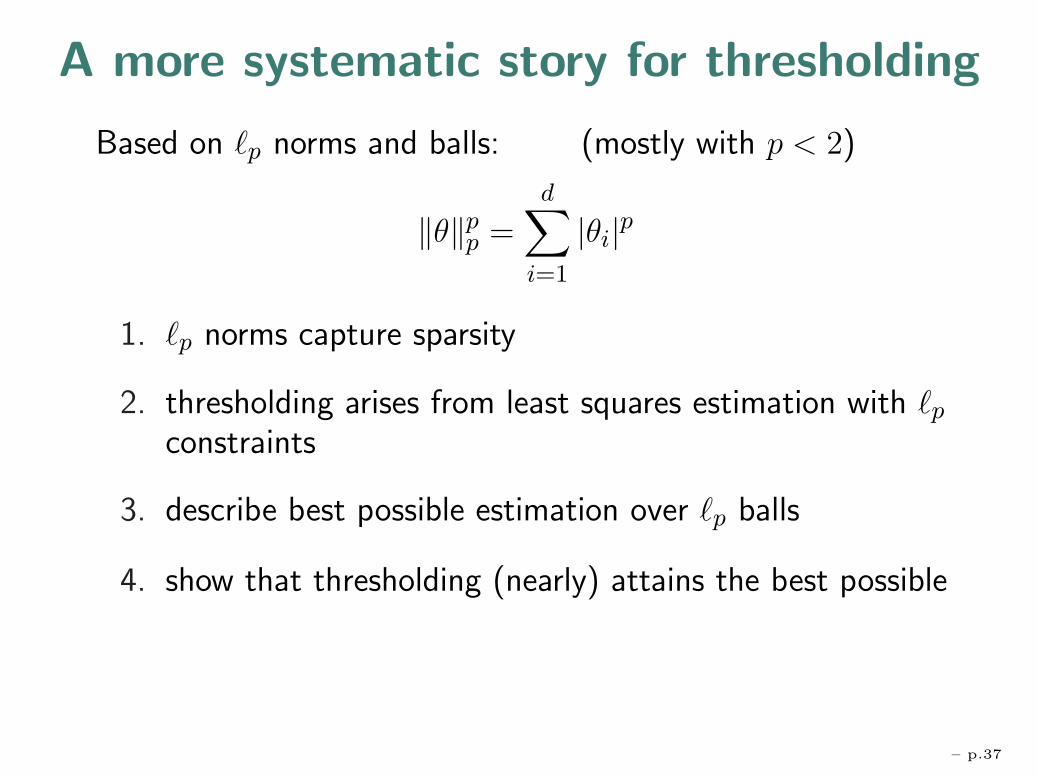
A more systematic story for thresholding
Based on p norms and balls: (mostly with p < 2)
‖θ‖pp =
d∑i=1
|θi|p
1. p norms capture sparsity
2. thresholding arises from least squares estimation with pconstraints
3. describe best possible estimation over p balls
4. show that thresholding (nearly) attains the best possible
– p.37

p norms, p < 2, capture sparsity
)(
1 ball smaller than 2, ⇒ expect better estimation
– p.38
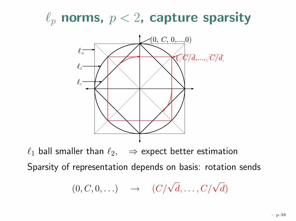
p norms, p < 2, capture sparsity
)(
1 ball smaller than 2, ⇒ expect better estimation
Sparsity of representation depends on basis: rotation sends
(0, C, 0, . . .) → (C/√d, . . . , C/
√d)
– p.38

Thresholding from constrained least squares
min∑
(yi − θi)2 s.t.
∑|θi|p ≤ Cp
i.e. min∑
(yi − θi)2 + λ|θi|p
leads to
• p = 2 Linear Shrinkage θi = (1 + λ)−1yi
• p = 1 Soft thresholding θi =
⎧⎪⎨⎪⎩yi − λ′ yi > λ′
0 |yi| ≤ λ′
yi + λ′ yi < −λ′[λ′ = λ/2]
• p = 0 Hard thresholding θi = yiI{|yi| > λ}.[ penalty λ
∑I{θi �= 0} ]
– p.39

Bounds on best estimation on p balls
Minimax risk: Rd,p(C) = infθsup‖θ‖p≤C Eθ
∑d1(θi − θi)
2.
Non-asymptotic bounds: [ Birge-Massart]
c1rd,p(C) ≤ Rd,p(C) ≤ c2[log d+ rd,p(C)]
• 1 ball smaller → (much) smaller minimax risk
– p.40

Bounds on best estimation on p balls
Minimax risk: Rd,p(C) = infθsup‖θ‖p≤C Eθ
∑d1(θi − θi)
2.
Non-asymptotic bounds: [ Birge-Massart]
c1rd,p(C) ≤ Rd,p(C) ≤ c2[log d+ rd,p(C)]
bound for thresholding
• 1 ball smaller → (much) smaller minimax risk
– p.40
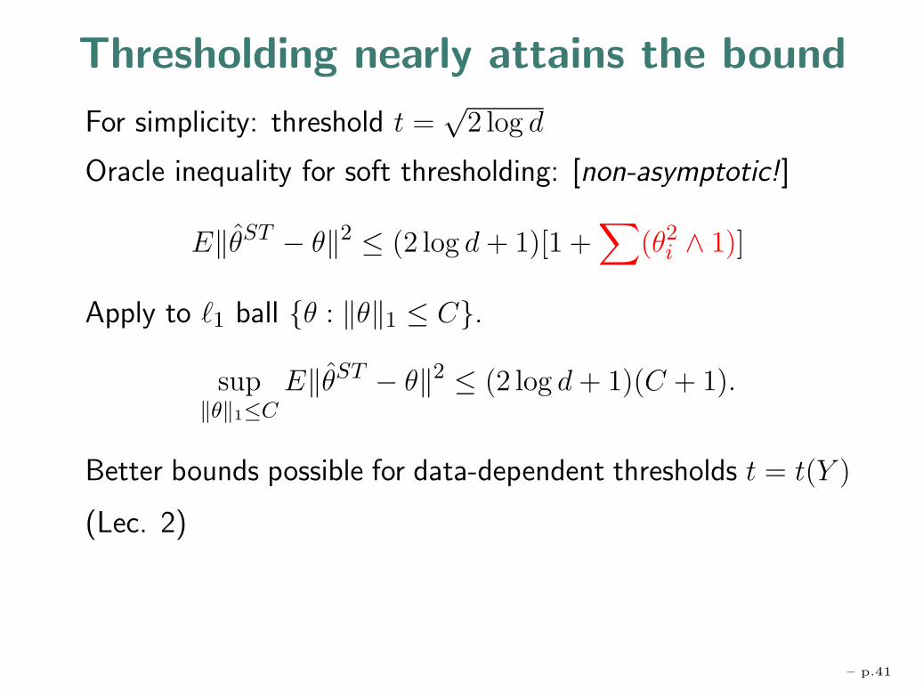
Thresholding nearly attains the bound
For simplicity: threshold t =√
2 log d
Oracle inequality for soft thresholding: [non-asymptotic!]
E‖θST − θ‖2 ≤ (2 log d+ 1)[1 +∑
(θ2i ∧ 1)]
Apply to 1 ball {θ : ‖θ‖1 ≤ C}.
sup‖θ‖1≤C
E‖θST − θ‖2 ≤ (2 log d+ 1)(C + 1).
Better bounds possible for data-dependent thresholds t = t(Y )
(Lec. 2)
– p.41

Summary for Nd(θ, I)
For X ∼ Nd(θ, I), comparing
• James Stein shrinkage (β = d− 2), and
• soft thresholding at t =√
2 log d:
James-Stein shrinkage: orthogonally invariant:
12(‖θ‖2 ∧ d) ≤ E‖θJS − θ‖2 ≤ 2 + (‖θ‖2 ∧ d)
Thresholding: co-ordinatewise, and co-ordinate dependent:
12
∑(θ2
i ∧ 1) ≤ E‖θST − θ‖2 ≤ (2 log d+ 1)(1 +∑
(θ2i ∧ 1))
– p.42

Implications for Function Estimation
Key example: functions of bounded total variation:TV (C) = {f : ‖f‖TV ≤ C}
‖f‖TV = supt1<...<tN
N−1∑i=1
|f(ti+1) − f(ti)| + ‖f‖1
Well captured by weighted combinations of 1 norms onwavelet coefficients:
c1 supj
2j/2‖θj‖1 ≤ ‖f‖TV ≤ c2∑
j
2j/2‖θj‖1
Best possible (minimax) MSE
R(TV (C), ε) = inff
supf∈TV (C)
E‖f − f‖2
– p.43

Reduction to single levels
supθE‖θ − θ‖2 =
∑j
supθj
E‖θj − θj‖2
• Apply thresholding bounds for eachj: to N2j(θj , ε
2I).
• ∃ a worst case level j∗ = j∗(ε, C),
• Geometric decay of supj E‖θj − θj‖2
as |j − j∗| ↗.
Growing Gaussian aspect: As noise ε = σ/√n) decreases,
worst level j∗ = j∗(ε, C) increases:
dj� = 2j∗ = c(C/ε)2/3
– p.44

Final Resultsup
TV (C)R(fthr, f) � C2(1−r)ε2r r = 2/3
supTV (C)
R(fJS, f) � C2(1−rL)ε2rL rL = 1/2
0 0.2 0.4 0.6 0.8 1−10
−5
0
5
10
15
20 Blocks signal
0 0.2 0.4 0.6 0.8 1−10
−5
0
5
10
15
20
25 Noisy version
0 0.2 0.4 0.6 0.8 1−10
−5
0
5
10
15
20
25\sqrt 2 log d threshold
0 0.2 0.4 0.6 0.8 1−10
−5
0
5
10
15
20
25Block JS shrinkage
– p.45

Agenda
• Classical Parametric Ideas
• Nonparametric Estimation and
Growing Gaussian Models
• I. Kernel Estimation and James-Stein Shrinkage
• II. Thresholding and Sparsity
• III. Bernstein-von Mises phenomenon
– p.46
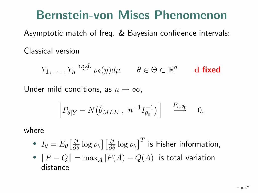
Bernstein-von Mises Phenomenon
Asymptotic match of freq. & Bayesian confidence intervals:
Classical version
Y1, . . . , Yni.i.d.∼ pθ(y)dµ θ ∈ Θ ⊂ R
d d fixed
Under mild conditions, as n→ ∞,∥∥∥Pθ|Y −N(θMLE , n−1I−1
θ0
)∥∥∥ Pn,θ0−→ 0,
where
• Iθ = Eθ
[∂∂θ log pθ
][∂∂θ log pθ
]Tis Fisher information,
• ‖P −Q‖ = maxA |P (A) −Q(A)| is total variationdistance
– p.47

Non-parametric Regression
Yi = f(i/n) + σ0wi, i = 1, . . . , n
For typical smoothness priors (e.g. dth integrated Wienerprocess prior)
• Bernstein - von Mises fails [Dennis Cox, D. A. Freedman]
• frequentist & posterior laws of ‖f − f‖22 mismatch in
center and scale
Here,
• revisit via elementary Growing Gaussian Model approach
• Apply to single levels of wavelet decomposition
– p.48

Growing Gaussian Model
Data: Y1, . . . , Yn|θ i.i.d.∼ Np(θ, σ20I) Prior: θ ∼ Np(0, τ
2n).
• growing: p = p(n) ↗ with n
• σ2n = Var(Yn|θ) = σ2
0/n; τ2n may depend on n.
Goal: compare L(θMLE|θ),L(θBayes|θ) with L(θ|Y ).
Posterior: All Gaussian: centering and scaling are key:
L(θ|Y = y
) ∼ Np
(θB = wny, wnσ
2nI
)
wn =τ2n
σ2n + τ2
n
– p.49

Growing Gaussians and BvM
Correspondences:
Pθ|Y ↔ Np(wny, wnσ2nI )
N(θMLE , n
−1I−1θ0
) ↔ Np( y, σ2nI )
For BvM to hold, now need wn ↗ 1 sufficiently fast:
Proposition: In the growing Gaussian model
∥∥Pθ|Y −N(θMLE , n
−1I−1θ0
)∥∥ Pn,θ0−→ 0,
if and only if
√pσ2
n
τ2n
=
√p
n
σ20
τ2n→ 0 i.e. wn = 1 − o
( 1√pn
).
– p.50

Example: Pinsker priors
Back to regression: dYt = f(t)dt+ σndWt
Minimax MSE linear estimation of f :
{f :
∫ 1
0(Dαf)2 ≤ C2 }
Least favourable prior on wavelet coeffs (for sample size n):
θjkindep∼ N(0, τ2
j )
τ2j = σ2
n(λn2−jα − 1)+
λn = c(C/σn)2α/(2α+1)
⇒ critical level j∗ = j∗(n, α) grows with n
(Growing Gaussian model again)
– p.51
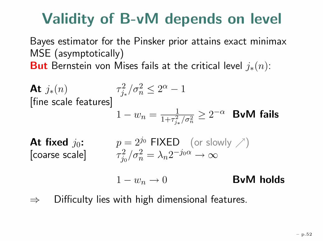
Validity of B-vM depends on level
Bayes estimator for the Pinsker prior attains exact minimaxMSE (asymptotically)But Bernstein von Mises fails at the critical level j∗(n):
At j∗(n) τ2j∗/σ
2n ≤ 2α − 1
[fine scale features]1 − wn = 1
1+τ2j∗/σ2
n≥ 2−α BvM fails
At fixed j0: p = 2j0 FIXED (or slowly ↗)[coarse scale] τ2
j0/σ2
n = λn2−j0α → ∞
1 − wn → 0 BvM holds
⇒ Difficulty lies with high dimensional features.
– p.52

Three Talks
1. Function Estimation & Classical Normal Theory• Xn ∼ Np(n)(θn, I) p(n) ↗ with n (MVN)
2. The Threshold Selection Problem• In (MVN) with, say, θi = XiI{|Xi| > t}• How to select t = t(X)“reliably”?
3. Large Covariance Matrices
• Xn ∼ Np(n)(I ⊗ Σp(n)); especially Xn =
[Yn
Zn
]
• spectral properties of n−1XnXTn
• PCA, CCA, MANOVA
– p.53