Embed Size (px)
Citation preview
Combined State and Parameter Reduction
(for Input-Output Systems)
Christian Himpe ([email protected])Mario Ohlberger ([email protected])
WWU Münster
Institute for Computational and Applied Mathematics
Exploratory Workshop on Applications of Model Order Reduction Methods
06.11.2015

Disclaimer
1 There will be no �ashy images.
2 There will be formulas.
Why Model Reduction?
My simulation is based on a model, ...
... that is large.
... that needs to be simulated many times.
... that has to be simulated in n seconds.
What it usually boils down to:�It takes too long!�
Popular Beliefs
1 �I just buy a faster computer.�
Moore's LawThe memory bottleneckResource coverage (DM, NUMA, SMP, SMT, SIMD, GPGPU)
2 �I just use a coarser grid.�
Detail ResolutionNumerical PropertiesInformation Disregard
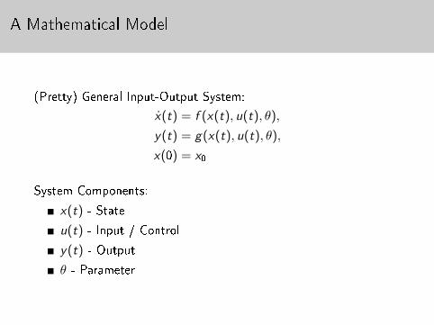
A Mathematical Model
(Pretty) General Input-Output System:
x(t) = f (x(t), u(t), θ),
y(t) = g(x(t), u(t), θ),
x(0) = x0
System Components:
x(t) - State
u(t) - Input / Control
y(t) - Output
θ - Parameter
One of Many Interpretations
x0 is a equilibrium state of the system.
u(t) is an external perturbation
to a system with dynamic behavor x(t).
y(t) is a measurement from a few sensors.
The Poster Child
Linear (Time-Invariant) System:
x(t) = Ax(t) + Bu(t),
y(t) = Cx(t) + Du(t),
x(0) = x0
In The Wild
Input-Output Systems are used in:
Industrial Control
Mechanics
Electro Dynamics
Fluid Dynamics
Reaction Networks
Neuro Imaging
Network Dynamics
...
Play It Again, Sam
Many-Query Settings:
Optimal Control
Model Predictive Control
Model Constraint Optimization
Inverse Problems
Sensitivity Analysis
�Uncertainty Quanti�cation�
Setting the Stage
Now, what means large?
High-Dimensional State-Space: dim(x(t))� 1
High-Dimensional Parameter-Space: dim(θ)� 1
(Input- and output-space are usually small.)
Enter MOR
Model Order Reduction (MOR):
Low-Dimensional State-Space: dim(xr (t))� dim(x(t))
Low-Dimensional Parameter-Space: dim(θr )� dim(θ)
Model Reduction Error1 ‖y − yr‖ � 1 (!)
1In a suitable norm.
Intermission I
What we use model order reduction (MOR) for:
Network Connectivity Reconstruction
(from neuroimaging data for brain connectivity analysis)
Intermission II
We have:
Low-dimensional time-series measurements
from a large network of known size,
which is controllably perturbed.
We want:
statistics
on the inter-node connectivity
(This is a bayesian inverse problem treated with model constraint optimization)
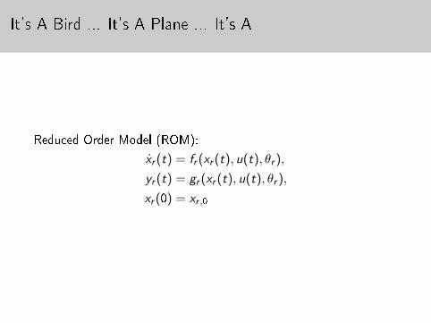
It's A Bird ... It's A Plane ... It's A
Reduced Order Model (ROM):
xr (t) = fr (xr (t), u(t), θr ),
yr (t) = gr (xr (t), u(t), θr ),
xr (0) = xr ,0
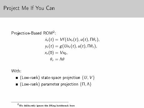
Project Me If You Can
Projection-Based ROM2:
xr (t) = Vf (Uxr (t), u(t),Πθr ),
yr (t) = g(Uxr (t), u(t),Πθr ),
xr (0) = Vx0,
θr = Λθ
With:
(Low-rank) state-space projection {U,V }(Low-rank) parameter projection {Π,Λ}
2We delibaretly ignore the lifting bottleneck here.
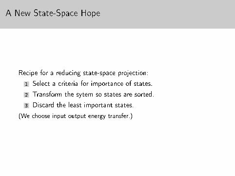
A New State-Space Hope
Recipe for a reducing state-space projection:
1 Select a criteria for importance of states.
2 Transform the sytem so states are sorted.
3 Discard the least important states.
(We choose input-output energy transfer.)
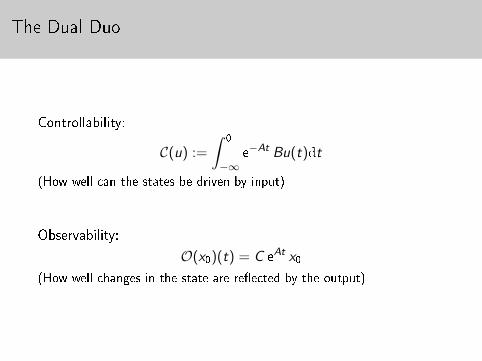
The Dual Duo
Controllability:
C(u) :=
∫ 0
−∞e−At Bu(t)dt
(How well can the states be driven by input)
Observability:
O(x0)(t) = C eAt x0
(How well changes in the state are re�ected by the output)
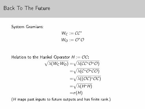
Back To The Future
System Gramians:
WC := CC∗
WO := O∗O
Relation to the Hankel Operator H := OC:√λ(WCWO) =
√λ(CC∗O∗O)
=√λ(C∗O∗CO)
=√λ((OC)∗OC)
=√λ(H∗H)
=σ(H)
(H maps past inputs to future outputs and has �nite rank.)
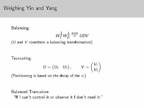
Weighing Yin and Yang
Balancing:
W12
C W12
OSVD= UDV
(U and V constitute a balancing transformation)
Truncating:
U =(U1 U2
), V =
(V1
V2
)(Partitioning is based on the decay of the σi )
Balanced Truncation:�If I can't control it or observe it I don't need it.�
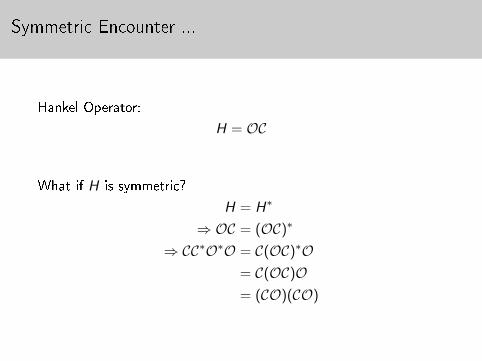
Symmetric Encounter ...
Hankel Operator:
H = OC
What if H is symmetric?
H = H∗
⇒ OC = (OC)∗
⇒ CC∗O∗O = C(OC)∗O= C(OC)O= (CO)(CO)
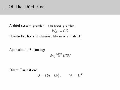
... Of The Third Kind
A third system gramian - the cross gramian:
WX := CO(Controllability and observability in one matrix!)
Approximate Balancing:
WXSVD= UDV
Direct Truncation:
U =(U1 U2
), V1 = UT
1
By Empirical Decree
How to compute these system gramians?
Solving matrix equations
Use empirical gramians (∗)
The Parameter-Space Strikes Back
Same recipe:
1 Select critera
2 Sort states
3 Discard tail
(Spoiler alert: We will use state-to-ouput in�uence)
A Parameter In A Tuxedo ...
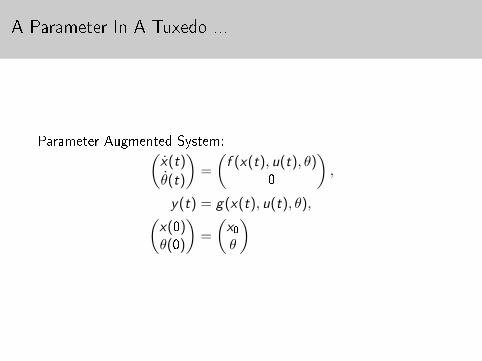
Parameter Augmented System:(x(t)
θ(t)
)=
(f (x(t), u(t), θ)
0
),
y(t) = g(x(t), u(t), θ),(x(0)θ(0)
)=
(x0θ
)
Double Cross
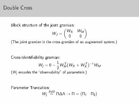
Block structure of the joint gramian:
WJ =
(WX WM
0 0
)(The joint gramian is the cross gramian of an augmented system.)
Cross-Identi�ability gramian:
WI = 0− 1
2W T
M (WX + W TX )−1WM
(WI encodes the �observability� of parameters.)
Parameter Truncation:
WISVD= Π∆Λ→ Π =
(Π1 Π2
)
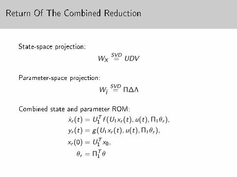
Return Of The Combined Reduction
State-space projection:
WXSVD= UDV
Parameter-space projection:
WISVD= Π∆Λ
Combined state and parameter ROM:
xr (t) = UT1 f (U1xr (t), u(t),Π1θr ),
yr (t) = g(U1xr (t), u(t),Π1θr ),
xr (0) = UT1 x0,
θr = ΠT1 θ
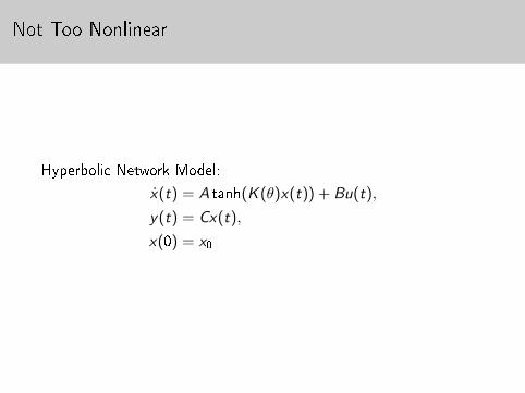
Not Too Nonlinear
Hyperbolic Network Model:
x(t) = A tanh(K (θ)x(t)) + Bu(t),
y(t) = Cx(t),
x(0) = x0
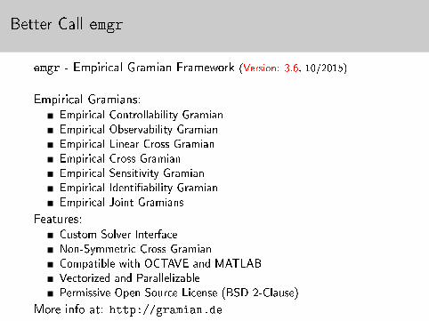
Better Call emgr
emgr - Empirical Gramian Framework (Version: 3.6, 10/2015)
Empirical Gramians:Empirical Controllability Gramian
Empirical Observability Gramian
Empirical Linear Cross Gramian
Empirical Cross Gramian
Empirical Sensitivity Gramian
Empirical Identi�ability Gramian
Empirical Joint Gramians
Features:Custom Solver Interface
Non-Symmetric Cross Gramian
Compatible with OCTAVE and MATLAB
Vectorized and Parallelizable
Permissive Open Source License (BSD 2-Clause)
More info at: http://gramian.de
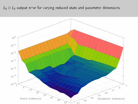
L2 ⊗ L2 output error for varying reduced state and parameter dimensions
1
9
17
25
33
41
49
57
1
9
17
25
33
41
49
57
10-6
10-5
10-4
10-3
10-2
10-1
100
Parameter DimensionState Dimension
tl;dl
Summary:
Combined state and parameter reduction
using empirical gramians
for nonlinear input-output systems.
wwwmath.uni-muenster.de/u/himpe
Thanks!
Get the Companion Code: j.mp/mornet15