Embed Size (px)
DESCRIPTION
The main goal of statistical phylogenetics is to reconstruct accurate phylogenies by means of comparison of nucleotide or protein sequences (i.e. DNA or Proteomics analysis). However, recent advances have shown that phylogenetics is not only related to taxonomy (i.e. data/species classification into categories) since different regions in nucleotide and protein sequences are subject to different evolutionary pressures or strains. Moreover, it is now apparent that different sequences accumulate substitutions at different rates (i.e. presence of inhomogeneities along sequences). Structural and functional constraints vary across sites of a protein. In other words, some protein sites may evolve slowly since most mutations ocurring at this particular site have low probabilities of being transmitted to descendants. For example, residues near the core of the molecule evolve under different processes than those exposed at the surface. The most dramatic example of this is related to the protein binding site dynamics, where the response of the cell depends on the binding nature of the cell receptors. In this case, one mutation in the core of the protein may turn an hallosterinc binding site into an orthosteric binding site and, therefore, the full response of the cell to a given receptor may be completely changed (for example, a severe infection turning into haemodynamic shock). From what has been said so far, it becomes apparent that the structural and functional constraints that shape protein evolution also affect substitution processes at the nucleotide level and vice versa. In this regard, two thirds of the nucleotide changes at the third codon position do not modify the amino acid translated (synonimous changes), whilst the mutations that take place at the second position systematically change the amino acid translated (non-synonimous changes). Also only 10\% of changes at the first codon position are synonimous so it can be concluded that evolutionary pressure varies depending on the constraints already present at the protein level. A simple approach to model this evolutionary feature is to allow the substition rates to vary across amino acid or nucleotide sites of the sequence. However, the estimation of the rate of change for each site of the alignment is impossible due to a combinatory explosion. In order to overcome this problem it is assumed that site rates are unknown but comply with a probabilistic distribution whose parameters or shape are estimated from the data. The structure of the genetic code is also responsible for other evolutionary patterns which are more complex than variations in rates across codon positions. Synonimous and non-synonimous mutations have varying probabilities of becoming `fixed' in a given population, which depends on the selective forces that act on the corresponding amino acids.
Citation preview

Modelling the Variability of Evolutionary Processes
Vicent RibasAlgebraic Models in Genomics
June 2010

Outline
1. Introduction• Molecular Clocks
2. Mathematical Models• Assumptions• Markov Models• Variability of Evolutionary Processes: Neyman (two-state), GTR and WAG• Trees and Likelihoods• Site Variability• Gamma-Based Rate across Sites• Markov Modulated Models (MMM)
3. Conclusions
Introduction
• Phylogenetics is not only related to taxonomy (i.e. data/species classification into categories) since different regions in nucleotide and protein sequences are subject to different evolutionary pressures or strains.• Structural and functional constraints vary across sites of a protein or DNA sequence.• The structural and functional constraints that shape protein evolution also affect substitution processes at the nucleotide level and vice versa.• Two thirds of the nucleotide changes at the third codon position do not modify the amino acid translated (synonimous changes), whilst the mutations that take place at the second position systematically change the amino acid translated (non-synonimous changes).• The structure of the genetic code is also responsible for other evolutionary patterns which are more complex than variations in rates across codon positions.• Synonimous and non-synonimous mutations have varying probabilities of becoming `fixed' in a given population, which depends on the selective forces that act on the corresponding amino acids. Non-synonimous changes modify the structure of the peptide being transcribed and alter its function (recall the hallosteric / orthosteric binding site example outlined above).
Introduction: Molecular Clocks
• It is normally assumed that the rate at which substitutions accumulate in proteins is constant over long periods of time.• The naïve implication of this fact results in the hypothesis that proteins could be used as “molecular clocks''. • Given a phylogenetic tree and a calibration point, it would be possible to date past evolutionary events. • Unfortunately, there are several clocks ticking at different times (Bergsonian Time).• Nowadays the most accurate molecular dating methods more or less relax the molecular clock constraint and rely instead on statistical models that describe the variations of substitution rates across lineages. • Most phylogenetic methods do not aim at estimating substitution rates but rather expected numbers of substitutions along each edge and, thus, produce non-clocklike trees.• A common assumption is that the expected amount of substitutions that acumulate on a given branch is the same at every site of the alignment. • The substitution rate on a given branch supposed to be constant across sites. Biological evidence suggests that some sites evolve quickly in some lineages and slowly in other clades, while different evolutionary patterns are observed at other sites.

Mathematical Models: Assumptions
• Aligned the sequences so as to extract homologous sites so that the dataset now comprises a set of sites where each site contains the character (nucleotide, amino acid, codon) of each of the sequences at a given position• Sites evolve independently.• Evolution has no memory, is time-continuous and time-homogeneous.• The evolutionary process is stationary.• The process is time-reversible.
La Leche League
• These assumptions imply that any model can be characterized by an instantaneous rate matrix Q, which remains constant during evolution
Mathematical Models: Markov Models
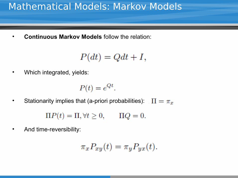
• Continuous Markov Models follow the relation:
• Which integrated, yields:
• Stationarity implies that (a-priori probabilities):
• And time-reversibility:

Mathematical Models: Variability of Evolutionary Models (Neyman Model)
• Neyman’s 2 state model:• Analyze DNA data, in which case the two states are Purine (R: A or G) and Pyrimidine (Y: C or T).• Express that sites can be in two different configurations (i.e. free to mutate or remain invariant). This case is the typical bistable configuration 'on' or 'off'. This version is suitable to study the heterogeneity of mutation rates over time and across sites.
• This model has just 1 free parameter

Mathematical Models: Variability of Evolutionary Models (GTR)
• General Time Reversible Model (GTR):• Applied to DNA models and it is a 4 state model (ACGT)
• Subject to: (10 parameters)
• Conservation of the Purine/Pyrimidine status yields:
• Transversions that transform Purine into Pyrimidine:

Mathematical Models: Variability of Evolutionary Models (Neyman Model)
• Neyman’s 2 state model:• Analyze DNA data, in which case the two states are Purine (R: A or G) and Pyrimidine (Y: C or T).• Express that sites can be in two different configurations (i.e. free to mutate or remain invariant). This case is the typical bistable configuration 'on' or 'off'. This version is suitable to study the heterogeneity of mutation rates over time and across sites.
• This model has just 1 free parameter

Mathematical Models: Variability of Evolutionary Models (GTR Simplified)
• Defining , which is estimated from data:
• Equal stationary probabilities result in the Kimura 2 Parameters Model (K2P).
• Assuming k=1, and equal stationary nucleotide frequencies results in the Jukes-Cantor Model, which does not require any parameter estimation.

Mathematical Models: Variability of Evolutionary Models (WAG Model)
• The WAG model applies to proteins and expresses the substitution rates of the 20 aminoacids.• It has been established from the analysis of a large number of protein families in a phylogenetic framework with ML methods.• The WAG symmetric matrix is given by:

Mathematical Models: Site Variability
• Sites in amino-acid or nucleotide sequences are subject to different evolutionary pressures and it is expected to find among-site variability in the rates and modes of evolution.• Sites belong to categories, which define an evolutionary mode and are fixed a-priori.• Two different situations are taken into consideration:
• the category of each site is known• the category of each site is unknown.

Mathematical Models: Markov Modultated Models
• The substitution process that governs the evolution of an individual site can now change time. • These category changes follow a homogeneous, stationary and time-reversible Markov process. • Here the states are the evolutionary categories instead of the sequence characters.• The stationary category distribution is given by:• And the GTR matrix becomes:
• δ governs the global rate of change between categories

Conclusions
• The main assumption of this work is that different regions in nucleotide and protein sequences are subject to different evolutionary pressures or strains.• This variability has been modelled by means of Continuous Markov models are characterized by an instantaneous rate matrix Q, which remains constant during evolution.• Different models to calculate this matrix Q have been presented. The most general one being the GTR (General Time Reversible).• Simplification of the GTR model results in different models studied in the course (K2P or JC as an example) by assuming, respectively:
• equal stationary probabilities (K2P)• equal stationary nucleotide frequencies and k=1 (JC).
• In regard to modelling the variability amongst proteomic sequences (peptides), the WAG model, which is widely used, has been presented.• Temporal variability is modelled by means of MMM.• This work is based on very strong assumptions (stationarity, time-reversibility, and independent evolution). • However, all these assumptions are necessary for the study, treatability and manageability of the models.• The models presented here have been successfully applied to the analysis of different sequences such as the HIV retrovirus envelope.