Structural Equation Modelling:Application using WVS data from selected Arab countries

Irina Vartanova

Institute for Futures Studies, Stockholm

ERF Workshop – May 12, 2015

1 / 20

Age and Attitudes towards Gender Equality

• According to modernization theory (Inglehart and Welzel,2005; Inglehart and Norris, 2003) young and well educatedpeople express greater support for gender equality

• The theory has been confirmed numerously in different worldregions

• Using the Arab Barometer data, Kostenko, Kuzmichev,Ponarin, 2014 found that the 25-34 group is the leastegalitarian in their gender attitudes

• Here we test whether the young are more supportive forgender equality using the 6 wave of WVS data

2 / 20

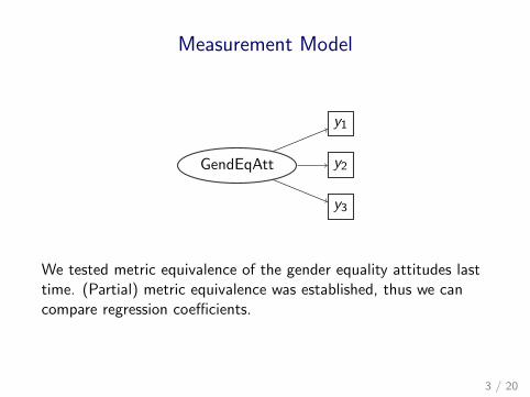
Measurement Model

GendEqAtt y2

y1

y3

We tested metric equivalence of the gender equality attitudes lasttime. (Partial) metric equivalence was established, thus we cancompare regression coefficients.

3 / 20

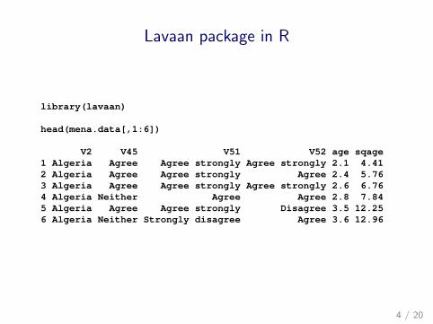
Lavaan package in R

library(lavaan)

head(mena.data[,1:6])

V2 V45 V51 V52 age sqage1 Algeria Agree Agree strongly Agree strongly 2.1 4.412 Algeria Agree Agree strongly Agree 2.4 5.763 Algeria Agree Agree strongly Agree strongly 2.6 6.764 Algeria Neither Agree Agree 2.8 7.845 Algeria Agree Agree strongly Disagree 3.5 12.256 Algeria Neither Strongly disagree Agree 3.6 12.96

4 / 20

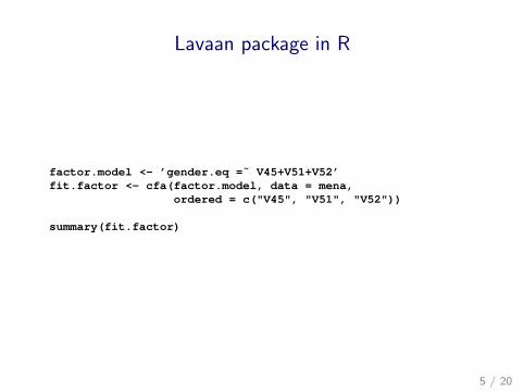
Lavaan package in R

factor.model <- ’gender.eq =˜ V45+V51+V52’fit.factor <- cfa(factor.model, data = mena,

ordered = c("V45", "V51", "V52"))

summary(fit.factor)

5 / 20

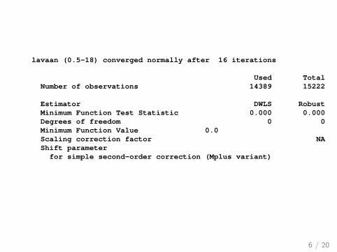
lavaan (0.5-18) converged normally after 16 iterations

Used TotalNumber of observations 14389 15222

Estimator DWLS RobustMinimum Function Test Statistic 0.000 0.000Degrees of freedom 0 0Minimum Function Value 0.0Scaling correction factor NAShift parameterfor simple second-order correction (Mplus variant)

6 / 20

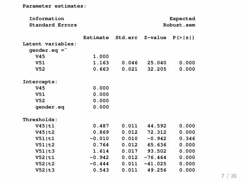
Parameter estimates:

Information ExpectedStandard Errors Robust.sem

Estimate Std.err Z-value P(>|z|)Latent variables:gender.eq =˜V45 1.000V51 1.163 0.046 25.040 0.000V52 0.663 0.021 32.205 0.000

Intercepts:V45 0.000V51 0.000V52 0.000gender.eq 0.000

Thresholds:V45|t1 0.487 0.011 44.592 0.000V45|t2 0.869 0.012 72.312 0.000V51|t1 -0.010 0.010 -0.942 0.346V51|t2 0.764 0.012 65.636 0.000V51|t3 1.614 0.017 93.502 0.000V52|t1 -0.942 0.012 -76.464 0.000V52|t2 -0.444 0.011 -41.025 0.000V52|t3 0.543 0.011 49.256 0.000

Variances:V45 0.575V51 0.425V52 0.814gender.eq 0.425 0.019

7 / 20

fitMeasures(fit.factor, c("chisq", "df", "pvalue", "cfi", "rmsea"))

chisq df pvalue cfi rmsea0 0 NA 1 0

8 / 20

Path diagrams in R

library(semPlot)

semPaths(fit.factor, title=FALSE, curvePivot = TRUE)semPaths(fit.factor,"std", edge.label.cex=0.5, curvePivot = TRUE)

9 / 20

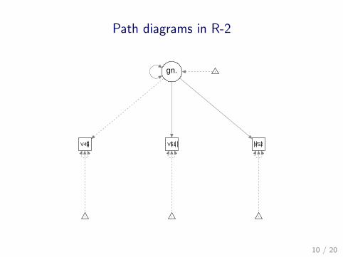
Path diagrams in R-2

V45 V51 V52

gn.

1 1 1

1

10 / 20

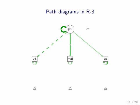
Path diagrams in R-3

0.43

0.43

0.58

0.65 0.76

0.81

1.00

V45 V51 V52

gn.

1 1 1

1

11 / 20

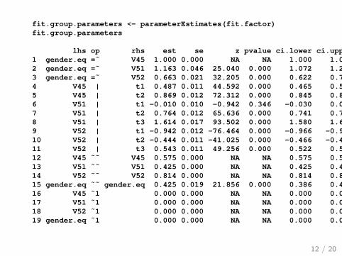
fit.group.parameters <- parameterEstimates(fit.factor)fit.group.parameters

lhs op rhs est se z pvalue ci.lower ci.upper1 gender.eq =˜ V45 1.000 0.000 NA NA 1.000 1.0002 gender.eq =˜ V51 1.163 0.046 25.040 0.000 1.072 1.2543 gender.eq =˜ V52 0.663 0.021 32.205 0.000 0.622 0.7034 V45 | t1 0.487 0.011 44.592 0.000 0.465 0.5085 V45 | t2 0.869 0.012 72.312 0.000 0.845 0.8926 V51 | t1 -0.010 0.010 -0.942 0.346 -0.030 0.0117 V51 | t2 0.764 0.012 65.636 0.000 0.741 0.7868 V51 | t3 1.614 0.017 93.502 0.000 1.580 1.6479 V52 | t1 -0.942 0.012 -76.464 0.000 -0.966 -0.91810 V52 | t2 -0.444 0.011 -41.025 0.000 -0.466 -0.42311 V52 | t3 0.543 0.011 49.256 0.000 0.522 0.56512 V45 ˜˜ V45 0.575 0.000 NA NA 0.575 0.57513 V51 ˜˜ V51 0.425 0.000 NA NA 0.425 0.42514 V52 ˜˜ V52 0.814 0.000 NA NA 0.814 0.81415 gender.eq ˜˜ gender.eq 0.425 0.019 21.856 0.000 0.386 0.46316 V45 ˜1 0.000 0.000 NA NA 0.000 0.00017 V51 ˜1 0.000 0.000 NA NA 0.000 0.00018 V52 ˜1 0.000 0.000 NA NA 0.000 0.00019 gender.eq ˜1 0.000 0.000 NA NA 0.000 0.000

12 / 20

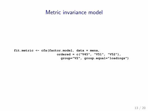
Metric invariance model

fit.metric <- cfa(factor.model, data = mena,ordered = c("V45", "V51", "V52"),group="V2", group.equal="loadings")

13 / 20

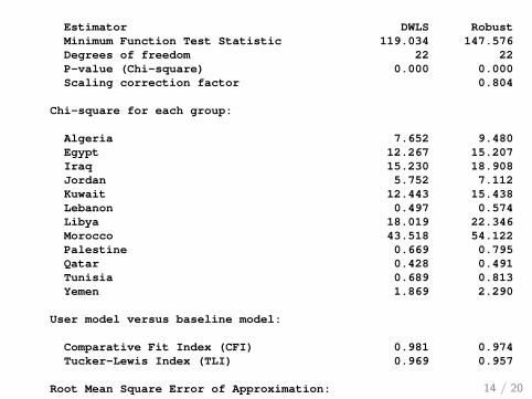
Estimator DWLS RobustMinimum Function Test Statistic 119.034 147.576Degrees of freedom 22 22P-value (Chi-square) 0.000 0.000Scaling correction factor 0.804

Chi-square for each group:

Algeria 7.652 9.480Egypt 12.267 15.207Iraq 15.230 18.908Jordan 5.752 7.112Kuwait 12.443 15.438Lebanon 0.497 0.574Libya 18.019 22.346Morocco 43.518 54.122Palestine 0.669 0.795Qatar 0.428 0.491Tunisia 0.689 0.813Yemen 1.869 2.290

User model versus baseline model:

Comparative Fit Index (CFI) 0.981 0.974Tucker-Lewis Index (TLI) 0.969 0.957

Root Mean Square Error of Approximation:

RMSEA 0.061 0.06990 Percent Confidence Interval 0.050 0.072 0.059 0.080P-value RMSEA <= 0.05 0.046 0.001

Weighted Root Mean Square Residual:

WRMR 3.290 3.290

14 / 20

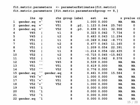
fit.metric.parameters <- parameterEstimates(fit.metric)fit.metric.parameters [fit.metric.parameters$group == 8,]

lhs op rhs group label est se z pvalue ci.lower ci.upper1 gender.eq =˜ V45 8 1.000 0.000 NA NA 1.000 1.0002 gender.eq =˜ V51 8 .p2. 1.123 0.044 25.760 0 1.038 1.2083 gender.eq =˜ V52 8 .p3. 0.698 0.021 32.908 0 0.656 0.7394 V45 | t1 8 0.323 0.042 7.734 0 0.241 0.4055 V45 | t2 8 0.483 0.043 11.294 0 0.399 0.5676 V51 | t1 8 -0.369 0.042 -8.773 0 -0.451 -0.2867 V51 | t2 8 0.477 0.043 11.165 0 0.394 0.5618 V51 | t3 8 1.209 0.054 22.391 0 1.103 1.3159 V52 | t1 8 -1.214 0.054 -22.435 0 -1.320 -1.10810 V52 | t2 8 -0.715 0.045 -15.863 0 -0.803 -0.62611 V52 | t3 8 0.360 0.042 8.578 0 0.278 0.44212 V45 ˜˜ V45 8 0.539 0.000 NA NA 0.539 0.53913 V51 ˜˜ V51 8 0.419 0.000 NA NA 0.419 0.41914 V52 ˜˜ V52 8 0.776 0.000 NA NA 0.776 0.77615 gender.eq ˜˜ gender.eq 8 0.461 0.030 15.584 0 0.403 0.51916 V45 ˜*˜ V45 8 1.000 0.000 NA NA 1.000 1.00017 V51 ˜*˜ V51 8 1.000 0.000 NA NA 1.000 1.00018 V52 ˜*˜ V52 8 1.000 0.000 NA NA 1.000 1.00019 V45 ˜1 8 0.000 0.000 NA NA 0.000 0.00020 V51 ˜1 8 0.000 0.000 NA NA 0.000 0.00021 V52 ˜1 8 0.000 0.000 NA NA 0.000 0.00022 gender.eq ˜1 8 0.000 0.000 NA NA 0.000 0.000

15 / 20

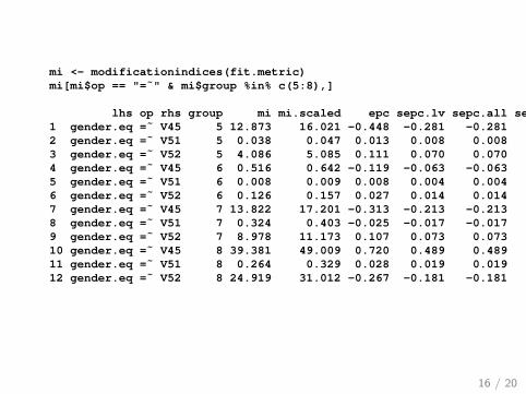
mi <- modificationindices(fit.metric)mi[mi$op == "=˜" & mi$group %in% c(5:8),]

lhs op rhs group mi mi.scaled epc sepc.lv sepc.all sepc.nox1 gender.eq =˜ V45 5 12.873 16.021 -0.448 -0.281 -0.281 -0.2812 gender.eq =˜ V51 5 0.038 0.047 0.013 0.008 0.008 0.0083 gender.eq =˜ V52 5 4.086 5.085 0.111 0.070 0.070 0.0704 gender.eq =˜ V45 6 0.516 0.642 -0.119 -0.063 -0.063 -0.0635 gender.eq =˜ V51 6 0.008 0.009 0.008 0.004 0.004 0.0046 gender.eq =˜ V52 6 0.126 0.157 0.027 0.014 0.014 0.0147 gender.eq =˜ V45 7 13.822 17.201 -0.313 -0.213 -0.213 -0.2138 gender.eq =˜ V51 7 0.324 0.403 -0.025 -0.017 -0.017 -0.0179 gender.eq =˜ V52 7 8.978 11.173 0.107 0.073 0.073 0.07310 gender.eq =˜ V45 8 39.381 49.009 0.720 0.489 0.489 0.48911 gender.eq =˜ V51 8 0.264 0.329 0.028 0.019 0.019 0.01912 gender.eq =˜ V52 8 24.919 31.012 -0.267 -0.181 -0.181 -0.181

16 / 20

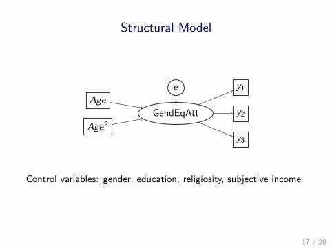
Structural Model

GendEqAtt y2

y1

y3

Age

Age2

e

Control variables: gender, education, religiosity, subjective income

17 / 20

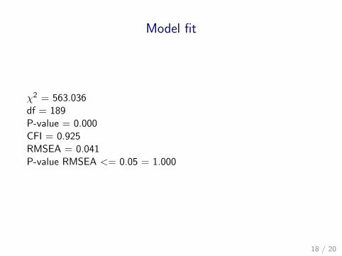
Model fit

χ2 = 563.036df = 189P-value = 0.000CFI = 0.925RMSEA = 0.041P-value RMSEA <= 0.05 = 1.000

18 / 20

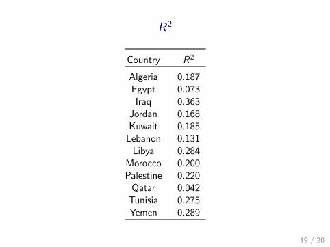
R2

Country R2

Algeria 0.187Egypt 0.073Iraq 0.363

Jordan 0.168Kuwait 0.185

Lebanon 0.131Libya 0.284

Morocco 0.200Palestine 0.220

Qatar 0.042Tunisia 0.275Yemen 0.289

19 / 20

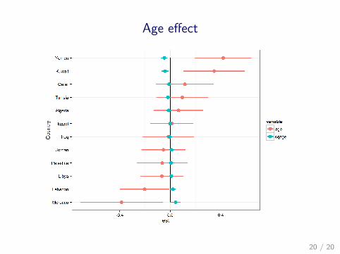
Age effect

20 / 20

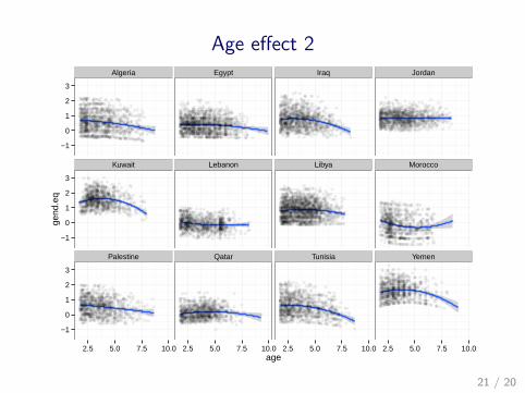
Age effect 2Algeria Egypt Iraq Jordan

Kuwait Lebanon Libya Morocco

Palestine Qatar Tunisia Yemen

−1

0

1

2

3

−1

0

1

2

3

−1

0

1

2

3

2.5 5.0 7.5 10.0 2.5 5.0 7.5 10.0 2.5 5.0 7.5 10.0 2.5 5.0 7.5 10.0age

gend

.eq

21 / 20