Structural Dynamic Reanalysis of Beam Elements Using Regression Method

IOSR Journal of Mechanical and Civil Engineering (IOSR-JMCE)

e-ISSN: 2278-1684,p-ISSN: 2320-334X, Volume 9, Issue 4 (Nov. - Dec. 2013), PP 50-58 www.iosrjournals.org

www.iosrjournals.org 50 | Page

Structural Dynamic Reanalysis of Beam Elements Using

Regression Method

P. Naga Latha1, P.SreenivasM.Tech

2

1(M.Tech-Student, Department of Mechanical Engineering, K.S.R.M.E.College/JNTUA, KADAPA, A.P.,INDIA ) 2(Assistant professor, Department of Mechanical Engineering, K.S.R.M.E.College, KADAPA, A.P.INDIA)

Abstract : This paper concerns with the reanalysis of Structural modification of a beam element based on

natural frequencies using polynomial regression method. This method deals with the characteristics of

frequency of a vibrating system and the procedures that are available for the modification of physical

parameters of vibrating structural system. The method is applied on a simple cantilever beam structure and T-

structure for approximate structural dynamic reanalysis. Results obtained from the assumed conditions of the

problem indicates the high quality approximation of natural frequencies using finite element method and

regression method.

Keywords: frequency, mass matrix, physical parameters, stiffness matrix, regression method.

I. INTRODUCTION Structural modification is usually having a technique to analyze the changes in the physical parameters

of a structural system on its dynamic characteristics. The physical parameters of a structural system are related

to the dynamic characteristics like mass, stiffness and damping properities.. for a spring- mass system, mass and

stiffness quantities are the physical properties for the elements. The parameters for a practical system such as a

cantilever beam and T-structure may be breadth, depth and length of a beam element. The changes in the

parameters will effect the dynamic characteristics i.e., both mass and stiffness properties of the beam . [1]

Reanalysis methods are intented to analyzeeffectively about the beam element structures that has been

modified due to changes in the design (or) while designing new structural elements. The source information may be utilized for the new designs. One of the many advantages of the elemental structure technique is, having the

possibility of repeating the analysis for one (or) more of the elements making the use of the work done by the

others. This will gives the most significant time saving when modifications are requried.[2]

Development of structural modification techniques which are them selves based on the previous

analysis. The modified matrices of the beam element structures are obtained , with little extra calculation time,

can be very easy and useful. The General structural modification techniques are very useful in solving medium

size structural problems as well as for the design of large structures also.

The main object is to evaluate the dynamic characteristics for such changes without solving the total

(or) complete set of modified equations.

II. Finite Element Approach Initially the total structure of the beam is divided into small elements using successive levels of

divisions. In finite element analysis more number of elements will give more accurate results especially of the

higher modes. The analysis of stiffness and mass matrix are performed for each element separately and then

globalized into a single matrix for the total system.

The generalized equations for the free vibration of the undamped system, is[3]

[M]𝑿 +[B]𝑿 +[K]x=f (1) Where M,B= αM+βK and K are the mass, damping and stiffness matrices respectively.

𝑋 ,𝑋 and X are acceleration, velocity, displacement vectors of the structural points and “f” is force

vector. Undamped homogeneous system of equation

M𝑿 +Kx=0 (2) Provides the Eigen value problem [K-λM] 𝝓 = 0 (3)

Such a system has natural frequencies

λ = 𝒘𝟏

𝟐 … …… … …… … 𝒘𝒏

𝟐

(4)

𝝓 = [𝝓1, 𝝓2….. 𝝓n ]

Structural Dynamic Reanalysis of Beam Elements Using Regression Method


Condition: Must satisfy the ortho normal conditions

𝝓𝑻M 𝝓=I,

𝝓𝑻K 𝝓=λ, (5)

𝝓𝑻C 𝝓 = αI+βλ=ξ,

It is important note, that the matrices,

𝑀 = 𝜙𝑇M 𝜙, 𝐶 = 𝜙𝑇C𝜙, 𝐾 = 𝜙𝑇K𝜙

Are not usually diagonalised by the eigenvectors of the original structure [4]

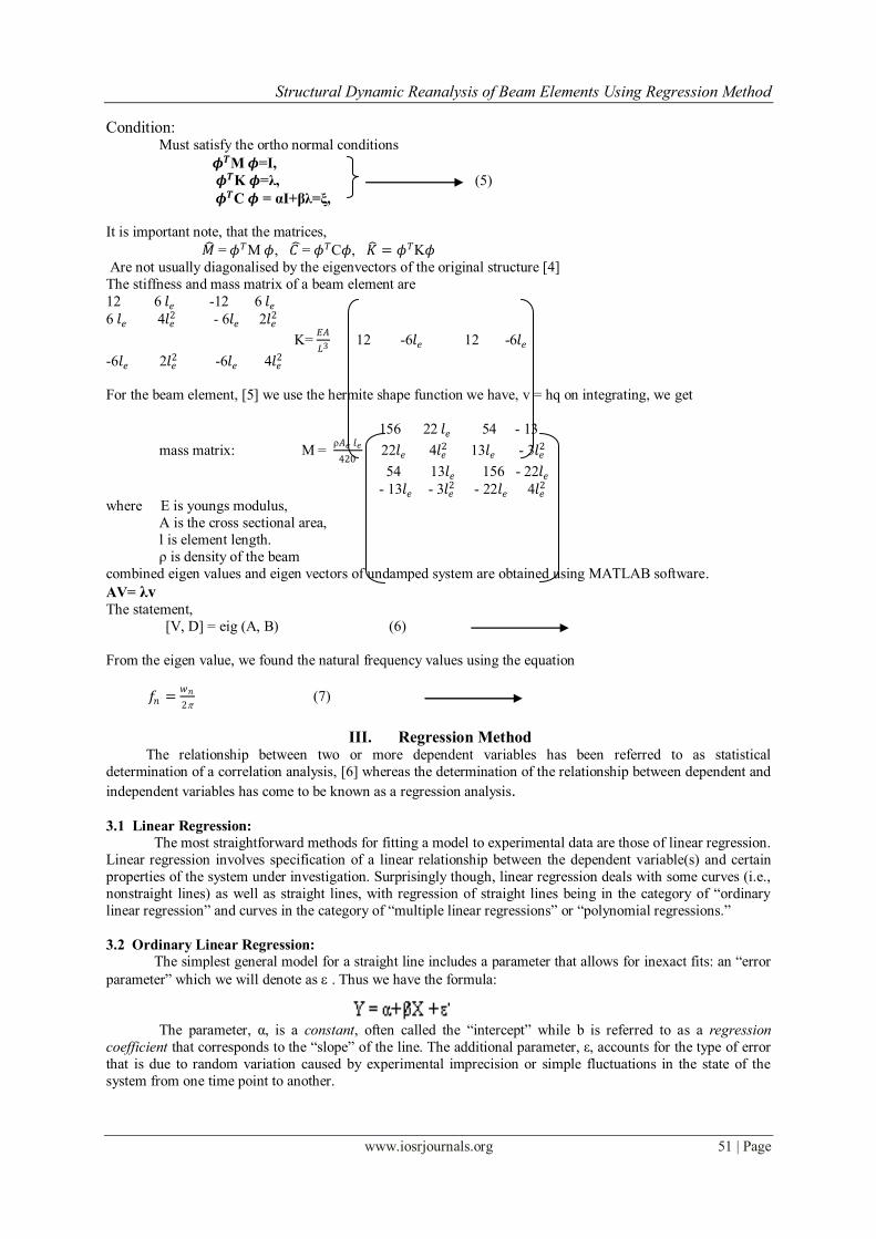
The stiffness and mass matrix of a beam element are

12 6 𝑙𝑒 -12 6 𝑙𝑒

6 𝑙𝑒 4𝑙𝑒2 - 6𝑙𝑒 2𝑙𝑒

2

K= 𝐸𝐴

𝐿3 12 -6𝑙𝑒 12 -6𝑙𝑒

-6𝑙𝑒 2𝑙𝑒2 -6𝑙𝑒 4𝑙𝑒

2

For the beam element, [5] we use the hermite shape function we have, v = hq on integrating, we get

156 22 𝑙𝑒 54 - 13

mass matrix: M = ρ𝐴𝑒 𝑙𝑒

420 22𝑙𝑒 4𝑙𝑒

2 13𝑙𝑒 - 3𝑙𝑒2

54 13𝑙𝑒 156 - 22𝑙𝑒

- 13𝑙𝑒 - 3𝑙𝑒2 - 22𝑙𝑒 4𝑙𝑒

2 where E is youngs modulus,

A is the cross sectional area,

l is element length.

ρ is density of the beam

combined eigen values and eigen vectors of undamped system are obtained using MATLAB software.

AV= λv The statement,

[V, D] = eig (A, B) (6)

From the eigen value, we found the natural frequency values using the equation

𝑓𝑛 =𝑤𝑛

2 (7)

III. Regression Method The relationship between two or more dependent variables has been referred to as statistical

determination of a correlation analysis, [6] whereas the determination of the relationship between dependent and

independent variables has come to be known as a regression analysis.

3.1 Linear Regression:

The most straightforward methods for fitting a model to experimental data are those of linear regression.

Linear regression involves specification of a linear relationship between the dependent variable(s) and certain

properties of the system under investigation. Surprisingly though, linear regression deals with some curves (i.e.,

nonstraight lines) as well as straight lines, with regression of straight lines being in the category of “ordinary

linear regression” and curves in the category of “multiple linear regressions” or “polynomial regressions.”

3.2 Ordinary Linear Regression:

The simplest general model for a straight line includes a parameter that allows for inexact fits: an “error

parameter” which we will denote as . Thus we have the formula:

The parameter, α, is a constant, often called the “intercept” while b is referred to as a regression

coefficient that corresponds to the “slope” of the line. The additional parameter, ε, accounts for the type of error

that is due to random variation caused by experimental imprecision or simple fluctuations in the state of the

system from one time point to another.



3.3 Multiple Linear Regressions:

The basic idea of the finite element method is piecewise approximation that is the solution of a

complicated problem is obtained by dividing the region of interest into small regions (finite element) and approximating the solution over each sub region by a simple function. Thus a necessary and important step is

that of choosing a simple function for the solution in each element. The functions used to represent the behavior

of the solution within an element are called interpolation functions or approximating functions or interpolation

models. Polynomial types of functions have been most widely used in the literature due to the following reasons.

(i) It is easier to formulate and computerize the finite element equations with polynomial functions. Specially

it is easier to perform differentiation or integration with polynomials.

(ii) It is possible to improve the accuracy of the results by increasing the order of the polynomial.

Theoretically a polynomial of infinite order corresponds to the exact solution. But in practice we use

polynomials of finite order only as an approximation.

The interpolation or shape functions are expressed in terms of natural coordinates. The representation of

geometry in terms of shape functions can be considered as a mapping procedure to calculate the natural frequency values for the variations of the physical properties.

Polynomial form of the shape functions for 1-D,2-D and 3-D elements are as follows:

𝛷 𝑥 = 𝛼1 + 𝛼2𝑥 + 𝛼3𝑥2 + ⋯ + 𝛼𝑚𝑥𝑛 (8)

𝛷 𝑥, 𝑦 = 𝛼1 + 𝛼2𝑥 + 𝛼3𝑦 + 𝛼4𝑥2 + 𝛼5𝑦

2 + 𝛼6𝑥𝑦…+ 𝛼𝑚𝑦𝑛 (9)

𝛷 𝑥, 𝑦, 𝑧 = 𝛼1 + 𝛼2𝑥 + 𝛼3𝑦 + 𝛼4𝑧 + 𝛼5𝑥2 + 𝛼6𝑦

2 + 𝛼7𝑧2 + 𝛼8𝑥𝑦 + 𝛼9𝑦𝑧 + 𝛼10𝑥𝑧… + 𝛼𝑚𝑧𝑛 (10)

3.4 Convergence Requirements:

Since the finite element method is a numerical technique, it obtains a sequence of approximate

solutions as the element size is reduced successively. The sequence will converge to the exact solution if the

polynomial function satisfies the following convergence requirements.

(i) The field variable must be continuous within the elements. This requirement is easily satisfied by

choosing continuous functions as regression models. Since polynomials are inherently type of regression

models as already discussed , satisfy the requriment.

(ii) All uniform states of the field variable „Φ‟ and its partial derivatitives upto the highest order appearing in the function (Φ) must have representation in the polynomial when, in the limit, the sizes are increased

(or) decreased successively.

(iii) The field variable „Φ‟ and its partial derivatives up to one order less than the highest order derivative

appearing in the field variable in the function (Φ) must be continuous at element boundaries or interfaces.

3.5 Non linear Regression:

A general model that encompasses all their behaviors cannot be defined in the sense used for

linear models, so we can use an explicit nonlinear function for illustrative purposes.

In this case, we will use the Hill equation:

Y = 𝛼 [𝐴]𝑠

[𝐴]𝑠+𝐾𝑠 (11)

Which contains one independent variable [A], and 3 parameters, α ,K, and S. Differentiating Y with respect to

each model parameter yields the following:

𝜕𝑦

𝜕𝛼 =

[𝐴]𝑠

[𝐴]𝑠+𝐾𝑠

𝜕𝑦

𝜕𝐾 =

−𝛼𝑠(𝐾[𝐴])𝑠

𝐾( [𝐴]𝑠+𝐾𝑠)2 (12)

𝜕𝑦

𝜕𝐾 =

−𝛼𝑠(𝐾[𝐴])𝑠

𝐾( [𝐴]𝑠+𝐾𝑠)2

All derivatives involve at least two of the parameters, so the model is nonlinear. However, it can be

seen that the partial derivative in equation 𝜕𝑦

𝜕𝛼 =

𝛼 [𝐴]𝑠

[𝐴]𝑠+𝐾𝑠 does not contain the parameter, α.

However the model is linear because the first derivatives do not include the parameters. As a consequence,

taking the second (or higher) order derivative of a linear function with respect to its parameters will always yield



a value of zero. Thus, if the independent variables and all but one parameter are held constant, the relationship

between the dependent variable and the remaining parameter will always be linear. It is important to note that

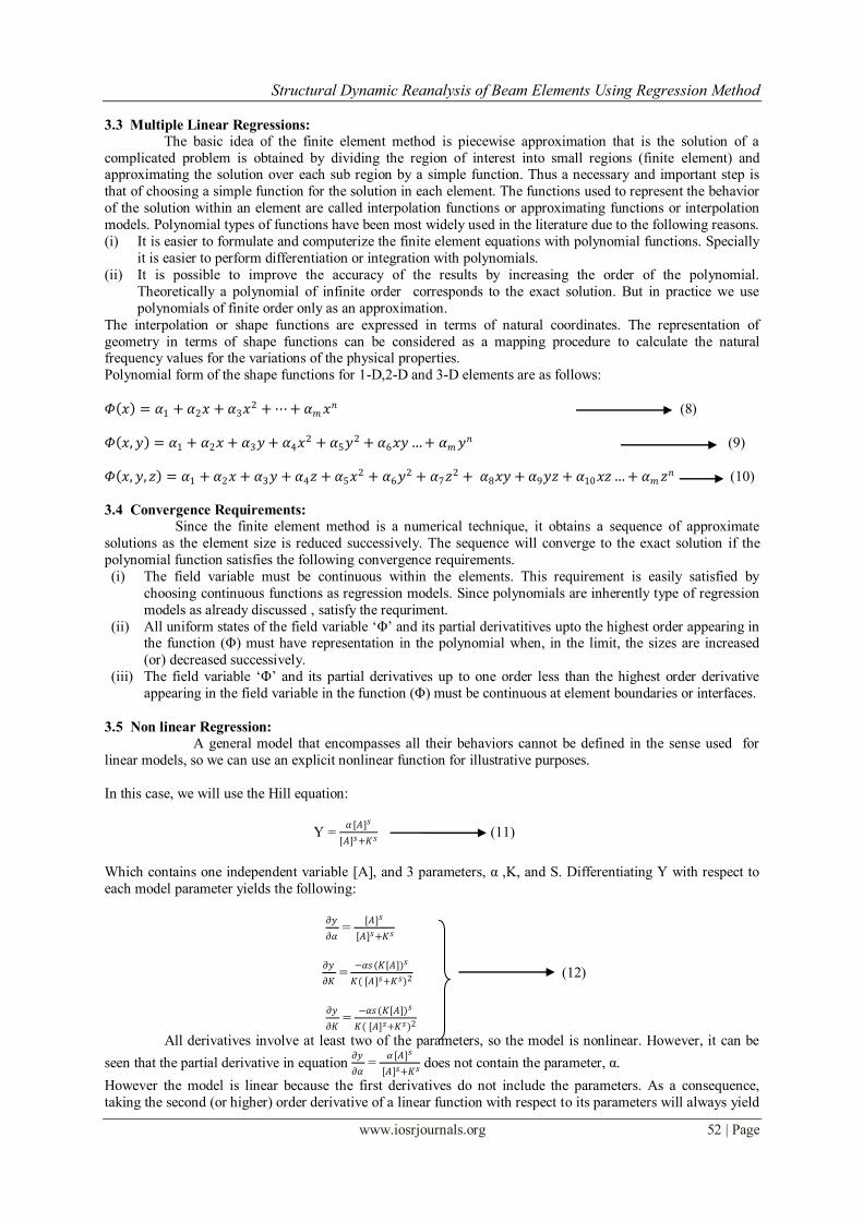
linear regression does not actually test whether the data sampled from the population follow a linear relationship. It assumes linearity and attempts to find the best-fit straight line relationship based on the data

sample. The dashed line shown in fig.(1) is the deterministic component, whereas the points represent the effect

of random error.

figure 1: a linear model that incorporates a stochastic (random error) component.

3.6 Assumptions of Standard Regression Analyses:

The subjects are randomly selected from a larger population. The same caveats apply here as with

correlation analyses.

1. The observations are independent.

2. X and Y are not interchangeable. Regression models used in the vast majority of cases attempt to predict the dependent variable, Y, from the independent variable, X and assume that the error in X is negligible. In

special cases where this is not the case, extensions of the standard regression techniques have been

developed to account for non negligible error in X.

3. The relationship between X and Y is of the correct form, i.e., the expectation function (linear or

nonlinear model) is appropriate to the data being fitted.

4. The variability of values around the line is Gaussian.

5. The values of Y have constant variance. Assumptions 5 and 6 are often violated (most particularly

when the data has variance where the standard deviation increases with the mean) and have to be specifically

accounted forin modifications of the standard regression procedures.

6. There are enough datapoints to provide a good sampling of the random error associated with the

experimental observations. In general, the minimum number of independent points can be no less than the number of parameters being estimated, and should ideally be significantly higher.

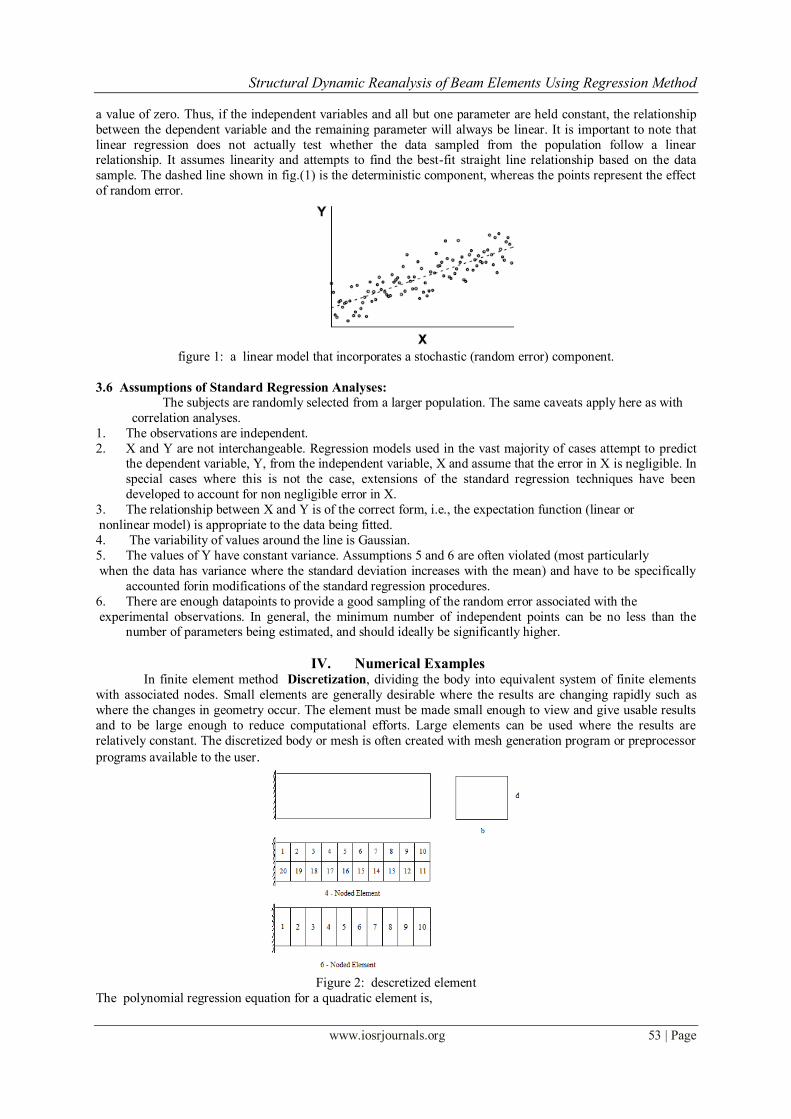
IV. Numerical Examples In finite element method Discretization, dividing the body into equivalent system of finite elements

with associated nodes. Small elements are generally desirable where the results are changing rapidly such as

where the changes in geometry occur. The element must be made small enough to view and give usable results

and to be large enough to reduce computational efforts. Large elements can be used where the results are

relatively constant. The discretized body or mesh is often created with mesh generation program or preprocessor

programs available to the user.

Figure 2: descretized element

The polynomial regression equation for a quadratic element is,



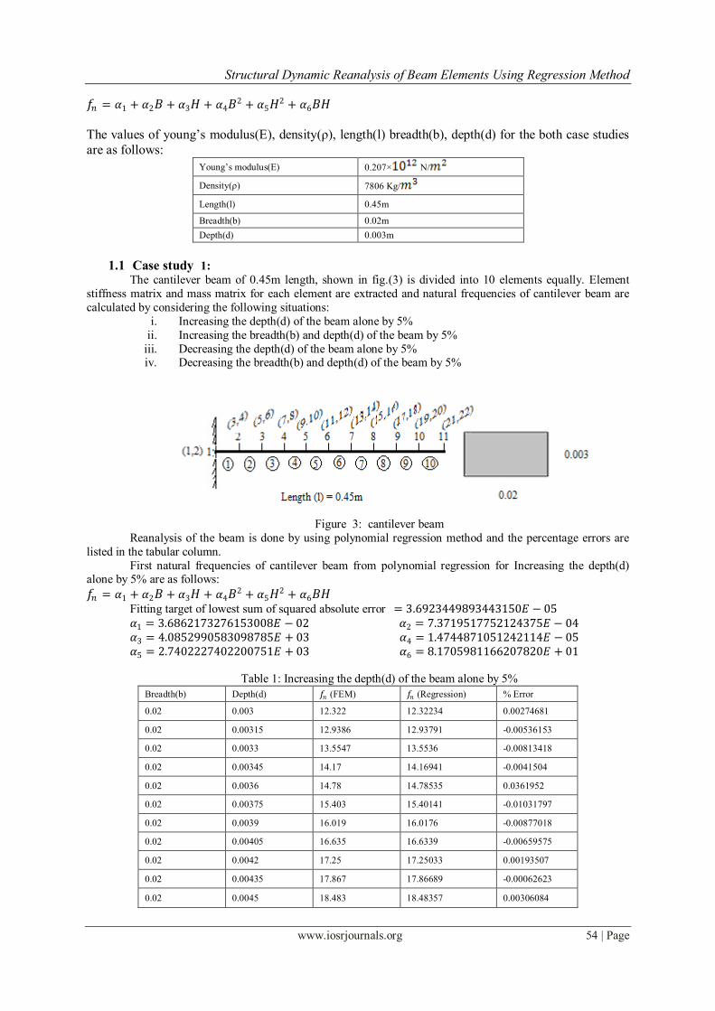
𝑓𝑛 = 𝛼1 + 𝛼2𝐵 + 𝛼3𝐻 + 𝛼4𝐵2 + 𝛼5𝐻

2 + 𝛼6𝐵𝐻

The values of young‟s modulus(E), density(ρ), length(l) breadth(b), depth(d) for the both case studies

are as follows:

Young‟s modulus(E) 0.207× N/

Density(ρ) 7806 Kg/

Length(l) 0.45m

Breadth(b) 0.02m

Depth(d) 0.003m

1.1 Case study 1:

The cantilever beam of 0.45m length, shown in fig.(3) is divided into 10 elements equally. Element

stiffness matrix and mass matrix for each element are extracted and natural frequencies of cantilever beam are

calculated by considering the following situations:

i. Increasing the depth(d) of the beam alone by 5%

ii. Increasing the breadth(b) and depth(d) of the beam by 5%

iii. Decreasing the depth(d) of the beam alone by 5% iv. Decreasing the breadth(b) and depth(d) of the beam by 5%

Figure 3: cantilever beam

Reanalysis of the beam is done by using polynomial regression method and the percentage errors are

listed in the tabular column.

First natural frequencies of cantilever beam from polynomial regression for Increasing the depth(d) alone by 5% are as follows:

𝑓𝑛 = 𝛼1 + 𝛼2𝐵 + 𝛼3𝐻 + 𝛼4𝐵2 + 𝛼5𝐻

2 + 𝛼6𝐵𝐻 Fitting target of lowest sum of squared absolute error = 3.6923449893443150𝐸 − 05

𝛼1 = 3.6862173276153008𝐸 − 02 𝛼2 = 7.3719517752124375𝐸 − 04

𝛼3 = 4.0852990583098785𝐸 + 03 𝛼4 = 1.4744871051242114𝐸 − 05

𝛼5 = 2.7402227402200751𝐸 + 03 𝛼6 = 8.1705981166207820𝐸 + 01

Table 1: Increasing the depth(d) of the beam alone by 5%

Breadth(b) Depth(d) 𝑓𝑛 (FEM) 𝑓𝑛 (Regression) % Error

0.02 0.003 12.322 12.32234 0.00274681

0.02 0.00315 12.9386 12.93791 -0.00536153

0.02 0.0033 13.5547 13.5536 -0.00813418

0.02 0.00345 14.17 14.16941 -0.0041504

0.02 0.0036 14.78 14.78535 0.0361952

0.02 0.00375 15.403 15.40141 -0.01031797

0.02 0.0039 16.019 16.0176 -0.00877018

0.02 0.00405 16.635 16.6339 -0.00659575

0.02 0.0042 17.25 17.25033 0.00193507

0.02 0.00435 17.867 17.86689 -0.00062623

0.02 0.0045 18.483 18.48357 0.00306084



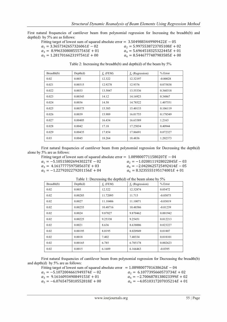
First natural frequencies of cantilever beam from polynomial regression for Increasing the breadth(b) and

depth(d) by 5% are as follows:

Fitting target of lowest sum of squared absolute error = 3.5049883449909422𝐸 − 05

𝛼1 = 3.3657342657326061𝐸 − 02 𝛼2 = 5.9975538723705108𝐸 + 02

𝛼3 = 8.9963308085557543𝐸 + 01 𝛼4 = 5.6964518325322445𝐸 + 01

𝛼5 = 1.2817016623197541𝐸 + 00 𝛼6 = 8.5446777487983585𝐸 + 00

Table 2: Increasing the breadth(b) and depth(d) of the beam by 5%


0.02 0.003 12.322 12.32197 -0.00028

0.021 0.00315 12.9278 12.9376 0.075838

0.022 0.0033 13.5047 13.55336 0.360318

0.023 0.00345 14.12 14.16923 0.34867

0.024 0.0036 14.58 14.78522 1.407551

0.025 0.00375 15.385 15.40133 0.106119

0.026 0.0039 15.989 16.01755 0.178549

0.027 0.00405 16.434 16.63389 1.2163

0.028 0.0042 17.18 17.25034 0.40944

0.029 0.00435 17.854 17.86691 0.072327

0.03 0.0045 18.264 18.4836 1.202373

First natural frequencies of cantilever beam from polynomial regression for Decreasing the depth(d)

alone by 5% are as follows:


𝛼1 = −5.1051580269430227𝐸 − 02 𝛼2 = −1.0208111928022845𝐸 − 03

𝛼3 = 4.1617777597585637𝐸 + 03 𝛼4 = −2.0420625725492414𝐸 − 05

𝛼5 = −1.2279202279201156𝐸 + 04 𝛼6 = 8.3235555195174001𝐸 + 01

Table 1: Decreasing the depth(d) of the beam alone by 5%


0.02 0.003 12.322 12.32874 0.05472

0.02 0.00285 11.72095 11.715 -0.05075

0.02 0.0027 11.10406 11.10071 -0.03019

0.02 0.00255 10.48716 10.48586 -0.01239

0.02 0.0024 9.87027 9.870462 0.001942

0.02 0.00225 9.25338 9.25451 0.012213

0.02 0.0021 8.636 8.638006 0.023227

0.02 0.00195 8.0195 8.020949 0.01807

0.02 0.0018 7.402 7.40334 0.018101

0.02 0.00165 6.785 6.785178 0.002623

0.02 0.0015 6.1689 6.166463 -0.0395

First natural frequencies of cantilever beam from polynomial regression for Decreasing the breadth(b)

and depth(d) by 5% are as follows:


𝛼1 = −5.1072004661949374𝐸 − 02 𝛼2 = 6.1077395660573734𝐸 + 02

𝛼3 = 9.1616093490849153𝐸 + 01 𝛼4 = −2.7006878138023399𝐸 + 02

𝛼5 = −6.0765475810552818𝐸 + 00 𝛼6 = −4.0510317207035214𝐸 + 01



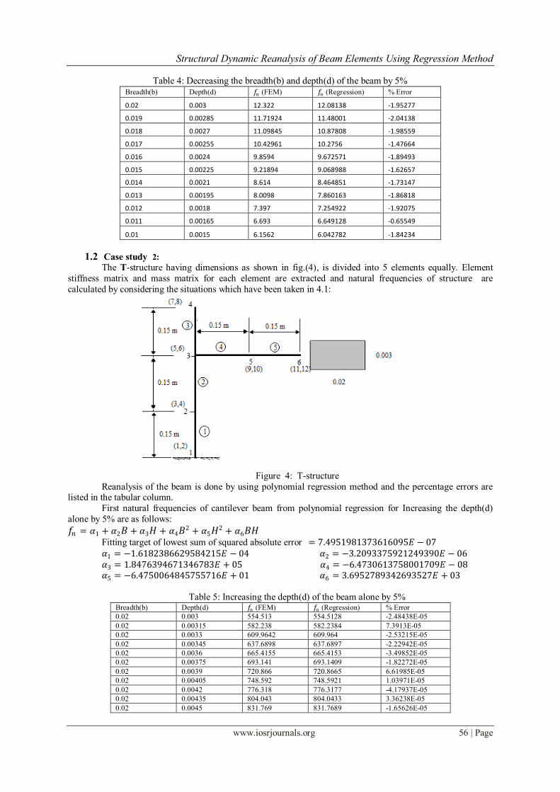
Table 4: Decreasing the breadth(b) and depth(d) of the beam by 5% Breadth(b) Depth(d) 𝑓𝑛 (FEM) 𝑓𝑛 (Regression) % Error

0.02 0.003 12.322 12.08138 -1.95277

0.019 0.00285 11.71924 11.48001 -2.04138

0.018 0.0027 11.09845 10.87808 -1.98559

0.017 0.00255 10.42961 10.2756 -1.47664

0.016 0.0024 9.8594 9.672571 -1.89493

0.015 0.00225 9.21894 9.068988 -1.62657

0.014 0.0021 8.614 8.464851 -1.73147

0.013 0.00195 8.0098 7.860163 -1.86818

0.012 0.0018 7.397 7.254922 -1.92075

0.011 0.00165 6.693 6.649128 -0.65549

0.01 0.0015 6.1562 6.042782 -1.84234

1.2 Case study 2:

The T-structure having dimensions as shown in fig.(4), is divided into 5 elements equally. Element

stiffness matrix and mass matrix for each element are extracted and natural frequencies of structure are

calculated by considering the situations which have been taken in 4.1:

Figure 4: T-structure

Reanalysis of the beam is done by using polynomial regression method and the percentage errors are listed in the tabular column.

First natural frequencies of cantilever beam from polynomial regression for Increasing the depth(d)


𝑓𝑛 = 𝛼1 + 𝛼2𝐵 + 𝛼3𝐻 + 𝛼4𝐵2 + 𝛼5𝐻

2 + 𝛼6𝐵𝐻 Fitting target of lowest sum of squared absolute error = 7.4951981373616095𝐸 − 07

𝛼1 = −1.6182386629584215𝐸 − 04 𝛼2 = −3.2093375921249390𝐸 − 06

𝛼3 = 1.8476394671346783𝐸 + 05 𝛼4 = −6.4730613758001709𝐸 − 08

𝛼5 = −6.4750064845755716𝐸 + 01 𝛼6 = 3.6952789342693527𝐸 + 03

Table 5: Increasing the depth(d) of the beam alone by 5% Breadth(b) Depth(d) 𝑓𝑛 (FEM) 𝑓𝑛 (Regression) % Error

0.02 0.003 554.513 554.5128 -2.48438E-05

0.02 0.00315 582.238 582.2384 7.3913E-05

0.02 0.0033 609.9642 609.964 -2.53215E-05

0.02 0.00345 637.6898 637.6897 -2.22942E-05

0.02 0.0036 665.4155 665.4153 -3.49852E-05

0.02 0.00375 693.141 693.1409 -1.82272E-05

0.02 0.0039 720.866 720.8665 6.61985E-05

0.02 0.00405 748.592 748.5921 1.03971E-05

0.02 0.0042 776.318 776.3177 -4.17937E-05

0.02 0.00435 804.043 804.0433 3.36238E-05

0.02 0.0045 831.769 831.7689 -1.65626E-05



First natural frequencies of cantilever beam from polynomial regression for Increasing the breadth(b) and

depth(d) by 5% are as follows:


𝛼1 = −1.6188811317291245𝐸 − 04 𝛼2 = 2.7115577353372031𝐸 + 04

𝛼3 = 4.0673366030058064𝐸 + 03 𝛼4 = 4.0673366030058064𝐸 + 00

𝛼5 = −3.2042541568134908𝐸 − 02 𝛼6 = −2.1361694378748552𝐸 − 04

Table 6: Increasing the breadth(b) and depth(d) of the beam by 5% Breadth(b) Depth(d) 𝑓𝑛 (FEM) 𝑓𝑛 (Regression) % Error

0.02 0.003 554.513 554.5128 -2.48438E-05

0.021 0.00315 582.238 582.2384 7.3913E-05

0.022 0.0033 609.9642 609.964 -2.53215E-05

0.023 0.00345 637.6898 637.6897 -2.22942E-05

0.024 0.0036 665.4155 665.4153 -3.49852E-05

0.025 0.00375 693.141 693.1409 -1.82272E-05

0.026 0.0039 720.866 720.8665 6.61985E-05

0.027 0.00405 748.592 748.5921 1.03971E-05

0.028 0.0042 776.318 776.3177 -4.17937E-05

0.029 0.00435 804.043 804.0433 3.36238E-05

0.03 0.0045 831.769 831.7689 -1.65626E-05

First natural frequencies of cantilever beam from polynomial regression for Decreasing the depth(d)



𝛼1 = 4.5098480533081574𝐸 − 04 𝛼2 = 92209871374071.032𝐸 − 06

𝛼3 = 1.8476295891899648𝐸 + 05 𝛼4 = 1.8039435190075892𝐸 − 07

𝛼5 = 2.0461020463086680𝐸 + 02 𝛼6 = 3.6952591783799307𝐸 + 03

Table 7: Decreasing the depth(d) of the beam alone by 5% Breadth(b) Depth(d) 𝑓𝑛 (FEM) 𝑓𝑛 (Regression) % Error

0.02 0.003 554.5128 554.5128 1.42609E-05

0.02 0.00285 526.787 526.7871 2.46623E-05

0.02 0.0027 499.0616 499.0614 -3.4071E-05

0.02 0.00255 471.336 471.3357 -5.53281E-05

0.02 0.0024 443.61 443.6101 1.30024E-05

0.02 0.00225 415.884 415.8844 9.26578E-05

0.02 0.0021 388.159 388.1587 -7.1562E-05

0.02 0.00195 360.433 360.4331 1.89521E-05

0.02 0.0018 332.7077 332.7074 -8.30757E-05

0.02 0.00165 304.982 304.9818 -6.94796E-05

0.02 0.0015 277.256 277.2562 5.83598E-05

First natural frequencies of cantilever beam from polynomial regression for Decreasing the breadth(b)

and depth(d) by 5% are as follows:


𝛼1 = 4.5116550270616755𝐸 − 04 𝛼2 = 2.7115432386684053𝐸 + 04

𝛼3 = 4.0673148580025731𝐸 + 03 𝛼4 = 4.5001969533233819𝐸 + 00

𝛼5 = 1.0125443144973012𝐸 − 01 𝛼6 = 6.7502954299811790𝐸 − 01

Table 8: Decreasing the breadth(b) and depth(d) of the beam by 5% Breadth(b) Depth(d) 𝑓𝑛 (FEM) 𝑓𝑛 (Regression) % Error

0.02 0.003 554.5128 554.5129 2.2536E-05

0.019 0.00285 526.787 526.7872 3.3373E-05

0.018 0.0027 499.0616 499.0615 -2.4877E-05

0.017 0.00255 471.336 471.3358 -4.5593E-05

0.016 0.0024 443.61 443.6101 2.3346E-05



0.015 0.00225 415.884 415.8844 0.00010369

0.014 0.0021 388.159 388.1588 -5.974E-05

0.013 0.00195 360.433 360.4331 3.1683E-05

0.012 0.0018 332.7077 332.7075 -6.9284E-05

0.011 0.00165 304.982 304.9818 -5.4434E-05

0.01 0.0015 277.256 277.2562 7.491E-05

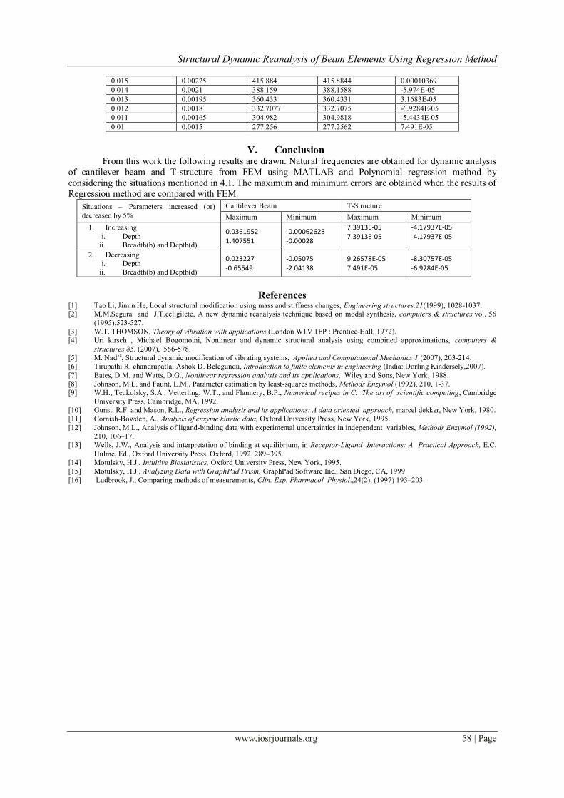
V. Conclusion From this work the following results are drawn. Natural frequencies are obtained for dynamic analysis

of cantilever beam and T-structure from FEM using MATLAB and Polynomial regression method by

considering the situations mentioned in 4.1. The maximum and minimum errors are obtained when the results of Regression method are compared with FEM.

Situations – Parameters increased (or)

decreased by 5%

Cantilever Beam T-Structure

Maximum Minimum Maximum Minimum

1. Increasing

i. Depth

ii. Breadth(b) and Depth(d)

0.0361952 1.407551

-0.00062623 -0.00028

7.3913E-05 7.3913E-05

-4.17937E-05 -4.17937E-05

2. Decreasing

i. Depth

ii. Breadth(b) and Depth(d)

0.023227 -0.65549

-0.05075 -2.04138

9.26578E-05 7.491E-05

-8.30757E-05 -6.9284E-05

References [1] Tao Li, Jimin He, Local structural modification using mass and stiffness changes, Engineering structures,21(1999), 1028-1037.

[2] M.M.Segura and J.T.celigilete, A new dynamic reanalysis technique based on modal synthesis, computers & structures,vol. 56

(1995),523-527. [3] W.T. THOMSON, Theory of vibration with applications (London W1V 1FP : Prentice-Hall, 1972).

[4] Uri kirsch , Michael Bogomolni, Nonlinear and dynamic structural analysis using combined approximations, computers &

structures 85, (2007), 566-578.

[5] M. Nad‟a, Structural dynamic modification of vibrating systems, Applied and Computational Mechanics 1 (2007), 203-214.

[6] Tirupathi R. chandrupatla, Ashok D. Belegundu, Introduction to finite elements in engineering (India: Dorling Kindersely,2007).

[7] Bates, D.M. and Watts, D.G., Nonlinear regression analysis and its applications, Wiley and Sons, New York, 1988.

[8] Johnson, M.L. and Faunt, L.M., Parameter estimation by least-squares methods, Methods Enzymol (1992), 210, 1-37.

[9] W.H., Teukolsky, S.A., Vetterling, W.T., and Flannery, B.P., Numerical recipes in C. The art of scientific computing, Cambridge

University Press, Cambridge, MA, 1992.

[10] Gunst, R.F. and Mason, R.L., Regression analysis and its applications: A data oriented approach, marcel dekker, New York, 1980.

[11] Cornish-Bowden, A., Analysis of enzyme kinetic data, Oxford University Press, New York, 1995.

[12] Johnson, M.L., Analysis of ligand-binding data with experimental uncertainties in independent variables, Methods Enzymol (1992),

210, 106–17.

[13] Wells, J.W., Analysis and interpretation of binding at equilibrium, in Receptor-Ligand Interactions: A Practical Approach, E.C.

Hulme, Ed., Oxford University Press, Oxford, 1992, 289–395.

[14] Motulsky, H.J., Intuitive Biostatistics, Oxford University Press, New York, 1995.

[15] Motulsky, H.J., Analyzing Data with GraphPad Prism, GraphPad Software Inc., San Diego, CA, 1999

[16] Ludbrook, J., Comparing methods of measurements, Clin. Exp. Pharmacol. Physiol.,24(2), (1997) 193–203.