Embed Size (px)
Citation preview

IOSR Journal of Mechanical and Civil Engineering (IOSR-JMCE)
e-ISSN: 2278-1684,p-ISSN: 2320-334X, Volume 13, Issue 5 Ver. V (Sep. - Oct. 2016), PP 01-14
www.iosrjournals.org
DOI: 10.9790/1684-1305050114 www.iosrjournals.org 1 | Page
Structural Dynamic Reanalysis of Cantilever Beam Using
Polynomial Regression Method
C.Srikarrao1, K.Kumar
2, P.Pavan Kumar
3, C. Mukul
4,P.Vinay
5
1,3,4,5(M.Tech-Student, Department of Mechanical Engineering, Jntuceh/Jntuh, Hyderabad, Telangana, India)
2(B.Tech, Mechanical Engineering)
Abstract: Reanalysis methods are intended to analyze efficiently structures that are modified due to changes in
the design. To find out the changes in the dynamic properties (natural frequency), solving of various
simultaneous equations for Eigen values is necessary and is a length, breadth and depth. In this paper, the focus
will be on reanalysis of a Cantilever beam. The natural frequency of the Cantilever beam will be calculated
using Ansys, FEM (using MAT LAB software) and also using conventional equations of Cantilever Beam. These
values are compared using polynomial regression method.
Keywords: frequency, mass matrix, physical parameters, stiffness matrix, regression method, ANSYS,
Reanalysis
I. Introduction Most optimal design procedures are iterative and require repeated analyses of structures obtained by
progressive modifications in design variables. Reanalysis methods are intended to analyze efficiently structures
that are modified due to changes in design. The object is to evaluate the structural modification within the frame
of vibration analysis technology refers to technique to modify physical properties of a structure in order to
change or optimize its dynamic properties. To find out the changes in the dynamic properties (natural
frequency), solving of various simultaneous equations for the Eigen values is necessary and is lengthy process.
To avoid this, changes in physical parameters are considered such as length, breadth and depth.
Reanalysis
Reanalysis methods are intended to analyze efficiently new designs using information from previous
ones. One of the many advantages of the substructure technique is the possibility of repeating the analysis for
one or more of the substructures making use of the work done on the others. This represents a significant saving
of time when modifications once are required. Modification is invariably required in iterative processes for
optimum design never the less, in the case of large structures the expenses are still too high. Therefore,
development of techniques which are themselves based on previous analysis, and which obtained the condensed
matrices of the substructures under modification, with little extra calculation time, can be very useful. “General
Reanalysis Techniques” are very useful in solving medium size problems and are totally essential in the design
of large structures. Some steps in a dynamic condensation process are particularly characterized by their
computational effort, as for instance:
1. Stiffness matrix factorization
2. Resolution of certain systems of linear equation
3. Resolution of an Eigen problem to obtain the normal vibration modes.
Reanalysis methods are intended to analyze efficiently structures that are modified due to changes in
the design. The object is to evaluate the structural response for such changes without solving the complete set of
modified simultaneous equations. The solution procedures usually use the original response of the structure.
Development of structural modification techniques which are themselves based on the previous analysis. The
modified matrices of the beam element structures are obtained, with little extra calculation time, can be very
easy and useful. The General structural modification techniques are very useful in solving medium size
structural problems as well as for the design of large structures also. The main object is to evaluate the dynamic
characteristics for such changes without solving the total (or) complete set of modified equations.
Finite Element Method Approach Initially the total structure of Cantilever beam is divided into small elements using successive levels of
divisions. In finite element analysis the structure is discredited into a set of elements joined together at some
points called nodes or nodal points. In analysis more number of elements will give more incisiveness results.
Assay of stiffness and mass matrix are performed for each element separately and then globalized into a single
matrix for the total system. The dynamic analysis of beam structure is [K-λM] [X]=0 ----------------- (1)

Structural Dynamic Reanalysis of Cantilever Beam Using Polynomial Regression Method
DOI: 10.9790/1684-1305050114 www.iosrjournals.org 2 | Page
Where k, m are the stiffness and mass matrix respectively. The dynamic behavior of a damped structure [4]
which is assumed to linear and discretized for n degrees of freedom can be described by the equation of motion.
M+C+Kx=f------------- (2)
Where M, C = αM+βK, and K are mass, damping and stiffness matrices, ,and X are acceleration, velocity,
displacement vectors of the structural points and “f” is force vector. Undamped homogeneous equation
M+Kx=0. Provides the Eigen value problem (k-λm) = 0.
Solution of above equation fetches the matrices eigen values λ and eigen vector Ɵ. 2
1
2
n
w
w
, 1 2[ , , , ]n
The eigen vector will satisfy the orthonormal conditions ,T M I ,T K ,TC I if
we use the transformation X q in the equation of motion, and premultiplying by T we get
T T T TM q C q K q f
-------------- (3).
It is vital note, that the matrices TM M , TC C , TK K
are not usually diagonalised by the eigenvectors of the original structure [3] Given an initial geometry Ŷand
assuming a change ΔY in the design variables, the modified design is given by Y Y Y -----------(4)
The geometric variables Y usually represent coordinates of joints, but other choice for thesevariables is
sometimes preferred. The displacement analysis equations for the initial design are Kr R . where K =
stiffness matrix corresponding to the designŶ , R= load vector whose elements are usually assumed to be
independent of the design variables and r= nodal displacements computedŶ at . The stiffness matrix and mass
matrix of a typical plane truss element are
2 2
3
2 2
12 6 12 6
6 4 6 2
6 612 12
6 62 4
e e
e e e e
e e
e ee e
l lEA
K l l l ll
l l
l ll l
and
2 2
2 2
156 22 54 13
22 4 13 3420
13 2254 156
13 223 4
e e
e ee e e e
e e
e ee e
l lA l
M l l l l
l l
l ll l
Where „A‟ is the cross sectional area of the cantilever beam, „l‟ is the length of the cantilever beam, „ρ‟ is the
density of the cantilever beam material
Regression Method
As with correlation, regression is used to analyze the relation between two continuous (scale) variables.
However, regression is better suited for studying functional dependencies between factors. The term functional
dependencyimplies that X [partially] determines the level of Y. For example, there is a function dependency
between age and Blood pressure since as one ages, blood pressure increases. In contrast, there is no functional
dependency between arms Length and leg length since increasing the length of an arm will have no effect on leg
length (or vice versa).In addition, regression is better suited than correlation for studying samples in which the
investigator fixes thedistribution of X. For example, if I decide to select ten 30-year-olds, ten 40-year olds, and
ten 50-year-olds to study the relation between age and blood pressure, I have fixed the distribution of the X
variable in the sample. This would necessitate the use of regression and (in theory) prevent the use of
Structural Dynamic Reanalysis of Cantilever Beam Using Polynomial Regression Method
DOI: 10.9790/1684-1305050114 www.iosrjournals.org 3 | Page
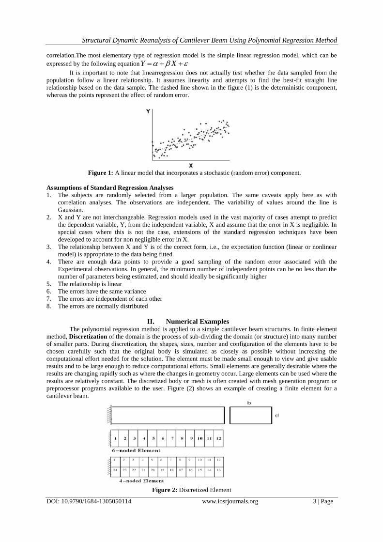
correlation.The most elementary type of regression model is the simple linear regression model, which can be
expressed by the following equationY X
It is important to note that linearregression does not actually test whether the data sampled from the
population follow a linear relationship. It assumes linearity and attempts to find the best-fit straight line
relationship based on the data sample. The dashed line shown in the figure (1) is the deterministic component,
whereas the points represent the effect of random error.
Figure 1: A linear model that incorporates a stochastic (random error) component.
Assumptions of Standard Regression Analyses 1. The subjects are randomly selected from a larger population. The same caveats apply here as with
correlation analyses. The observations are independent. The variability of values around the line is
Gaussian.
2. X and Y are not interchangeable. Regression models used in the vast majority of cases attempt to predict
the dependent variable, Y, from the independent variable, X and assume that the error in X is negligible. In
special cases where this is not the case, extensions of the standard regression techniques have been
developed to account for non negligible error in X.
3. The relationship between X and Y is of the correct form, i.e., the expectation function (linear or nonlinear
model) is appropriate to the data being fitted.
4. There are enough data points to provide a good sampling of the random error associated with the
Experimental observations. In general, the minimum number of independent points can be no less than the
number of parameters being estimated, and should ideally be significantly higher
5. The relationship is linear
6. The errors have the same variance
7. The errors are independent of each other
8. The errors are normally distributed
II. Numerical Examples The polynomial regression method is applied to a simple cantilever beam structures. In finite element
method, Discretization of the domain is the process of sub-dividing the domain (or structure) into many number
of smaller parts. During discretization, the shapes, sizes, number and configuration of the elements have to be
chosen carefully such that the original body is simulated as closely as possible without increasing the
computational effort needed for the solution. The element must be made small enough to view and give usable
results and to be large enough to reduce computational efforts. Small elements are generally desirable where the
results are changing rapidly such as where the changes in geometry occur. Large elements can be used where the
results are relatively constant. The discretized body or mesh is often created with mesh generation program or
preprocessor programs available to the user. Figure (2) shows an example of creating a finite element for a
cantilever beam.
Figure 2: Discretized Element

Structural Dynamic Reanalysis of Cantilever Beam Using Polynomial Regression Method
DOI: 10.9790/1684-1305050114 www.iosrjournals.org 4 | Page
The polynomial equation for regression method, 2 2
1 2 3 4 5 6nf C C B C H C B C H C BH
These 3 values for the case study Young‟s modulus (E) 205x109 N/m2
Density (ρ) 7850Kg/m3
Cross section of area (A) 0.0756m2
Dynamic Reanalysis Of Cantilever Beam Using Conventional Equations:
9.1 Free Vibration Analysis of Beams using Conventional Equations:
he conventional equations for cantilever beam based on the mode shapes are given as follows:
The first three undamped natural frequencies and mode shapes of cantilever beam
Case study :
A cantilever beam of 1.93m length, 0.252m breadth(b) and 0.3m depth(d) is shown in above
figure(3.2). The first mode of natural frequency values are calculated using conventional equation by
considering the following situations:
1. Increasing the depth(d) of the beam by 5%
2. Increasing the breadth(b) and depth(d) of the beam by 5%
3. Decreasing the depth(d) of the beam by 5%
4. Decreasing the breadth(b) and depth(d) by 5%
Fig. Cantilever Beam

Structural Dynamic Reanalysis of Cantilever Beam Using Polynomial Regression Method
DOI: 10.9790/1684-1305050114 www.iosrjournals.org 5 | Page
conventional results from first mode natural frequency formula:
The first mode of natural frequencies are obtained using conventional equation and the reanalysis of the beam is
done by using polynomial regression method and the percentage errors are calculated.
2
4(1.875)n
EI
mL
For our paperL=1.93m, b=0.252 m, d=0.3m
Therefore ,
Young‟s Modulu‟s, 9 2205 10E N m
Moment of inertia,
34
12
bdI m =0.000567
Area, A=0.0756
Density, 37850Kg m
Hence,
9
2
4
205 10 0.0005671.875
7850 0.0756 1.93n
=417.6963305 rad/sec
=66.478 Hz
Increasing the depth(d) of beam by 5%
By using the polynomial regression method the natural frequencies of cantilever beam for increasing the
depth(d) by 5% are as follows:
ƒ𝑛 =α1+ α2b+ α3d+ α4b2+ α5d
2+ α6bd
α1= -9.4658492835519595E-02 α2= -2.3853940192537948E-02
α3= 2.0884918091567624E+02 α4= -6.0111929279216270E-03
α5= -6.5545449365670549E-01 α6= 5.2629993590750750E+01
Table 3.3.1: Increasing the depth of beam by 5% Breadth(b) Depth(d) ƒn (Conventional) ƒn (Regression) %Error
0.252 0.3 66.47 66.47354 -0.05806
0.252 0.315 69.80235751 69.79917 -0.05523
0.252 0.33 73.12627928 73.12451 -0.05311
0.252 0.345 76.45020107 76.44955 -0.05154
0.252 0.36 79.77412285 79.7743 -0.05047
0.252 0.375 83.09804464 83.09875 -0.04984
0.252 0.39 86.42196642 86.42291 -0.0496
0.252 0.405 89.74588821 89.74677 -0.04971
0.252 0.42 93.06980999 93.07034 -0.05013
0.252 0.435 96.39373178 96.39361 -0.05082
0.252 0.45 99.71765357 99.71659 -0.05176
Increasing the breadth(b) and depth(d) of the beam by 5%
By using the polynomial regression method the natural frequencies of cantilever beam for increasing the
breadth(b) and depth(d) by 5% are as follows:
ƒ𝑛 =α1+ α2b+ α3d+ α4b2+ α5d
2+ α6bd
α1= 1.6257664335197344E-02 α2= 1.0908943441650720E+02
α3= 1.2986837430536571E+02 α4= 3.9719636556959870E-02
α5= 5.6292001923083035E-02 α6=4.7285281615472741E-02
Increasing the breadth(b) and depth(d) by 5%
Breadth(b) Depth(d) ƒn (Conventional) ƒn (Regression) %Error
0.252 0.3 66.51215 66.47847 -0.05064
0.2646 0.315 69.83776 69.80217 -0.05097
0.2772 0.33 73.16337 73.12592 -0.05119
0.2898 0.345 76.48898 76.44973 -0.05131
0.3024 0.36 79.81459 79.77359 -0.05136
0.315 0.375 83.14019 83.09751 -0.05134

Structural Dynamic Reanalysis of Cantilever Beam Using Polynomial Regression Method
DOI: 10.9790/1684-1305050114 www.iosrjournals.org 6 | Page
Decreasing the depth(d) of the beam by 5%
By using the polynomial regression method the natural frequencies of cantilever beam for decreasing the
depth(d) by 5% are as follows:
ƒ𝑛 =α1+ α2b+ α3d+ α4b2+ α5d
2+ α6bd
α1= -3.2325620284851558E-02 α2= -8.1460563085897775E-03
α3= 2.0868197121130873E+02 α4= -2.0528061901838868E-03
α5= -5.4208754208936583E-01α6=5.2587856745250306E+01
Decreasing the depth(d) of the beam by 5% Breadth(b) Depth(d) ƒn (Conventional) ƒn (Regression) %Error
0.252 0.3 66.47 66.47354 -0.05806
0.252 0.285 63.18655 63.17268 -0.02194
0.252 0.27 59.86094 59.84818 -0.02131
0.252 0.255 56.53533 56.52344 -0.02103
0.252 0.24 53.20972 53.19845 -0.02118
0.252 0.225 49.88412 49.87322 -0.02184
0.252 0.21 46.55851 46.54775 -0.02311
0.252 0.195 43.2329 43.22203 -0.02514
0.252 0.18 39.90729 39.89607 -0.02813
0.252 0.165 36.58168 36.56986 -0.03232
0.252 0.15 33.25608 33.24341 -0.03809
Decreasing the Breadth(b) and Depth(d) of the beam by 5%
By using the polynomial regression method the natural frequencies of cantilever beam for decreasing the
breadth(b) and depth(d) by 5% are as follows:
ƒ𝑛 =α1+ α2b+ α3d+ α4b2+ α5d
2+ α6bd
α1= -4.0920431654701064E+00 α2= -2.7795014096424597E+02
α3= 4.8636570319929723E+02 α4= -3.4603540586310110E+03
α5= -3.4474950483908215E+03 α6=6.9409522011659174E+03
Decreasing the Breadth(b) and Depth(d) of the beam by 5% Breadth(b) Depth(d) ƒn (Conventional) ƒn (Regression) %Error
0.252 0.3 66.51215 66.48934 -0.0343
0.2394 0.285 63.18655 63.2113 0.03918
0.2268 0.27 59.86094 59.90684 0.076683
0.2142 0.255 56.53533 56.57596 0.071858
0.2016 0.24 53.20972 53.21865 0.016769
0.189 0.225 49.88412 49.83491 -0.09864
0.1674 0.21 46.55851 46.51493 -0.0936
0.1548 0.195 43.2329 43.23057 -0.00539
0.1422 0.18 39.90729 39.91978 0.031292
0.1296 0.165 36.58168 36.58257 0.002415
0.117 0.15 33.25608 33.21893 -0.1117
Dynamic Analysis Of Cantilever Beam Using Ansys
Free Vibration Analysis of Beams using ANSYS:
0.3276 0.39 86.4658 86.42149 -0.05125
0.3402 0.405 89.79141 89.74552 -0.05111
0.3528 0.42 93.11702 93.06961 -0.05091
0.3654 0.435 96.44262 96.39375 -0.05068
0.378 0.45 99.76823 99.71795 -0.0504

Structural Dynamic Reanalysis of Cantilever Beam Using Polynomial Regression Method
DOI: 10.9790/1684-1305050114 www.iosrjournals.org 7 | Page
Beam under free Vibration
Modal Analysis:
Any physical system can vibrate. The frequencies at which vibration naturally occurs, and the modal
shapes which the vibrating system assumes are properties of the system, and can be determined analytically
using Modal Analysis.Analysis of vibration modes is a critical component of a design, but is often overlooked.
Structural elements such as complex steel floor systems can be particularly prone to perceptible vibration,
irritating building occupants or disturbing sensitive equipment. Inherent vibration modes in structural
components or mechanical support systems can shorten equipment life, and cause premature or completely
unanticipated failure, oftenresulting in hazardous situations. Detailed fatigue analysis is often required to assess
the potential for failure or damage resulting from the rapid stress cycles of vibration.
Detailed seismic qualification also requires an understanding of the natural vibration modes of a
system, as the large amount of energy acting on a system during seismic activity varies with frequency.The goal
of modal analysis in structural mechanics is to determine the natural mode shapes and frequencies of an object
or structure during free vibration. It is common to use the finite element method (FEM) to perform this analysis
because, like other calculations using the FEM, the object being analyzed can have arbitrary shape and the
results of the calculations are acceptable. The types of equations which arise from modal analysis are those seen
in eigensystems. The physical interpretation of theeigenvalues and eigenvectors which come from solving the
system are that they represent the frequencies and corresponding mode shapes. Sometimes, the only desired
modes are the lowest frequencies because they can be the most prominent modes at which the object will
vibrate, dominating all the higher frequency modes. It is also possible to test a physical object to determine its
natural frequencies and mode shapes. This is called an Experimental Modal Analysis. The results of the physical
test can be used to calibrate a finite element model to determine if the underlying assumptions made were
correct (for example, correct material properties and boundary conditions were used).
Procedure for modal in ANSYS
1. Build the model of cantilever beam as shown in figure 4.1
2. Define the material properties such as young‟s modulus and density etc.,
3. Apply boundary conditions
4. Enter the ANSYS solution processor in which analysis type is taken as modal analysis, and by taking
mode extraction method, by defining number of modes to be extracted.
5. Solve the problem using current LS command from the tool bar.
Here eigen values analysis of cantilever beam was carried out.
Physical Properties:
The physical properties of the beam are taken as follows:
Physical Properties Young‟s modulus(E) 205×109 N/m2
Density(ρ) 7850 Kg/m3
Length(l) 1.93m
Breadth(b) 0.252m
Depth(d) 0.3m
Case study:
A cantilever beam of length 1.93m, breadth(b) of 0.252m and depth(d) of 0.3m shown in figure(4.1) is
divided into 12 elements equally. Natural frequencies of the cantilever beam are calculated by considering the
following situations:

Structural Dynamic Reanalysis of Cantilever Beam Using Polynomial Regression Method
DOI: 10.9790/1684-1305050114 www.iosrjournals.org 8 | Page
1. Increasing the depth(d) of the beam by 5%
2. Increasing the breadth(b) and depth(d) of the beam by 5%
3. Decreasing the depth(d) of the beam by 5%
4. Decreasing the breadth(b) and depth(d) of the beam by 5%
L=1.93m, b=0.252 m, d=0.3m
Figure : Cantilever beam
Results from ANSYS for case study:
The Modal analysis of cantilever beam has been carried out by using ANSYS10.0
Increasing the depth(d) of the beam by 5%
By using ANSYS software the results for natural frequency for increasing the depth of the cantilever beam by
5% are calculated.
ƒ𝑛 = α1+ α2b+ α3d+ α4b2+ α5d
2+ α6bd
α1= -5.0991185667651062E-01α2= -1.2849778788034882E-01
α3= 2.1262898807318032E+02α4= -3.2381442545194261E-02
α5= -1.2442372442372843E+01α6= 5.3582504994441798E+01
ANSYS answer for table 4.4.1(under lined in table)
Increasing the depth(d) of the beam by 5% Breadth(b) Depth(d) ƒn(ANSYS) ƒn (Regression) %Error
0.252 0.3 66.177 66.17537 -0.00246
0.252 0.315 69.452 69.45257 0.000816
0.252 0.33 72.723 72.72416 0.001599
0.252 0.345 75.989 75.99016 0.001528
0.252 0.36 79.25 79.25056 0.000706
0.252 0.375 82.506 82.50536 -0.00078
0.252 0.39 85.755 85.75456 -0.00051
0.252 0.405 88.999 88.99816 -0.00094
0.252 0.42 92.237 92.23616 -0.00091
0.252 0.435 95.469 95.46857 -0.00045
0.252 0.45 98.694 98.69537 0.001389

Structural Dynamic Reanalysis of Cantilever Beam Using Polynomial Regression Method
DOI: 10.9790/1684-1305050114 www.iosrjournals.org 9 | Page
Increasing the breadth(b) and depth(d) of the beam by 5%
From the ANSYS the results of natural frequency for increasing the breadth and depth of cantilever beam by 5%
are calculated.
ƒ𝑛 = α1+ α2b+ α3d+ α4b2+ α5d
2+ α6bd
α1= -1.1349090909091647E+01 α2= 1.4024644664279012E+02
α3= 1.6696005552713106E+02α4= -2.8701379021631737E+01
α5= -4.0676557570339845E+01α6= -3.4168308359085330E+01
ANSYS answer for
Table 4.4.2(under lined in table)
Increasing the breadth(b) and depth(d) of the beam by 5% Breadth(b) Depth(d) ƒn(ANSYS) ƒn (Regression) %Error
0.252 0.3 66.177 66.01436 -0.24576
0.2646 0.315 69.452 69.45904 0.010131
0.2772 0.33 72.723 72.86338 0.193028
0.2898 0.345 76.149 76.22738 0.102932
0.3024 0.36 79.25 79.55105 0.37988
0.315 0.375 82.506 82.83439 0.398024
0.3276 0.39 87.304 86.0774 -1.40498
0.3402 0.405 88.999 89.28007 0.315816
0.3528 0.42 92.237 92.44241 0.2227
0.3654 0.435 95.469 95.56442 0.099947
0.378 0.45 98.694 98.64609 -0.04854
Decreasing the depth(d) of the beam by5%
From ANSYS the results of natural frequency for decreasing the depth of the cantilever beam by 5% are
calculated.
ƒ𝑛 = α1+ α2b+ α3d+ α4b2+ α5d
2+ α6bd
α1= -1.1399224458860556E-01 α2= -2.8726045128877331E-02
α3= 2.0995566247864440E+02α4= -7.2389633729237346E-03
α5= -7.6094276094307034E+00α6= 5.2908826944618909E+01
Structural Dynamic Reanalysis of Cantilever Beam Using Polynomial Regression Method
DOI: 10.9790/1684-1305050114 www.iosrjournals.org 10 | Page
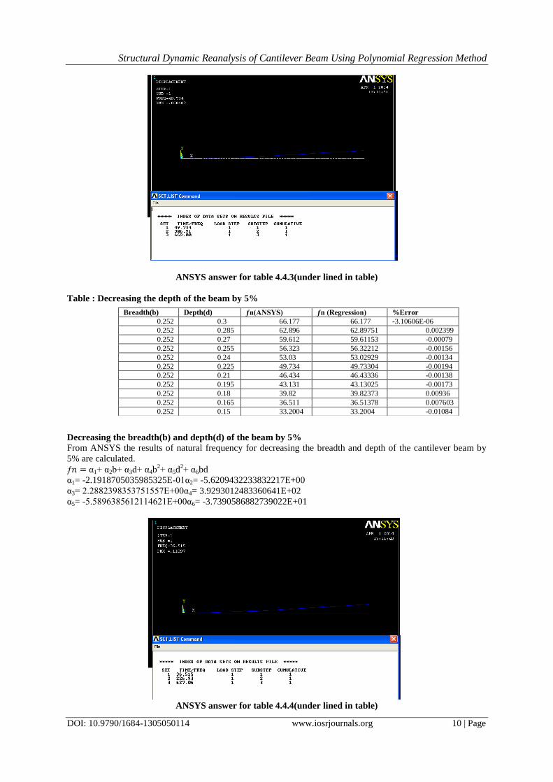
ANSYS answer for table 4.4.3(under lined in table)
Table : Decreasing the depth of the beam by 5%
Decreasing the breadth(b) and depth(d) of the beam by 5%
From ANSYS the results of natural frequency for decreasing the breadth and depth of the cantilever beam by
5% are calculated.
ƒ𝑛 = α1+ α2b+ α3d+ α4b2+ α5d
2+ α6bd
α1= -2.1918705035985325E-01α2= -5.6209432233832217E+00
α3= 2.2882398353751557E+00α4= 3.9293012483360641E+02
α5= -5.5896385612114621E+00α6= -3.7390586882739022E+01
ANSYS answer for table 4.4.4(under lined in table)
Breadth(b) Depth(d) ƒn(ANSYS) ƒn (Regression) %Error
0.252 0.3 66.177 66.177 -3.10606E-06
0.252 0.285 62.896 62.89751 0.002399
0.252 0.27 59.612 59.61153 -0.00079
0.252 0.255 56.323 56.32212 -0.00156
0.252 0.24 53.03 53.02929 -0.00134
0.252 0.225 49.734 49.73304 -0.00194
0.252 0.21 46.434 46.43336 -0.00138
0.252 0.195 43.131 43.13025 -0.00173
0.252 0.18 39.82 39.82373 0.00936
0.252 0.165 36.511 36.51378 0.007603
0.252 0.15 33.2004 33.2004 -0.01084

Structural Dynamic Reanalysis of Cantilever Beam Using Polynomial Regression Method
DOI: 10.9790/1684-1305050114 www.iosrjournals.org 11 | Page
Table: Decreasing the breadth(b) and depth(d) of the beam by 5% Breadth(b) Depth(d) ƒn(ANSYS) ƒn (Regression) %Error
0.252 0.3 66.177 66.177 -3.10606E-06
0.2394 0.285 62.896 62.89683 0.001318021
0.2268 0.27 59.612 59.61249 0.000817551
0.2142 0.255 56.327 56.32397 -0.005373847
0.2016 0.24 53.03 53.03129 0.002425279
0.189 0.225 49.734 49.73443 0.000857594
0.1674 0.21 46.434 46.43307 -0.002001758
0.1548 0.195 43.131 43.13173 0.001691351
0.1422 0.18 39.824 39.82622 0.00556405
0.1296 0.165 36.515 36.51653 0.00418868
0.117 0.15 33.204 33.20267 -0.004004025
Dynamic Analysis Of Cantilever Beam Usingfinite Element Method
Free vibration Analysis of the Beam using Finite Element
Method:
The polynomial regression method is applied to a simple beam structures. In finite element method,
Discretization means dividing the body into an equivalent system of finite elements with associated nodes. The
element must be made small enough to view and give usable results and to be large enough to reduce
computational efforts. Small elements are generally desirable where the results are changing rapidly such as
where the changes in geometry occur. Large elements can be used where the results are relatively constant. The
discretized body or mesh is often created with mesh generation program or pre-processor programs available to
the user. Figure shows an example of creating a finite element for a cantilever beam.
Discretized Element
The values of young‟s modulus(E), density(ρ), length(l), breadth(b), depth(d) for the case study are follows:
Table: Element Properties Young‟s modulus(E) 205×109
Density(ρ) 7850 Kg/m2
Length(l) 1.93m
Breadth(b) 0.252m
Depth(d) 0.3m
Case study:
A cantilever beam of length 1.93m, breadth(b) of 0.252m and depth(d) of 0.3m shown in figure(4.1) is
divided into 12 elements equally. Natural frequencies of the cantilever beam are calculated by considering the
following situations:
1. Increasing the depth(d) of the beam by 5%
2. Increasing the breadth(b) and depth(d) of the beam by 5%
3. Decreasing the depth(d) of the beam by 5%
4. Decreasing the breadth(b) and depth(d) of the beam by 5%
5.
L=1.93m, b=0.252 m, d=0.3m
FIG: Cantilever Beam

Structural Dynamic Reanalysis of Cantilever Beam Using Polynomial Regression Method
DOI: 10.9790/1684-1305050114 www.iosrjournals.org 12 | Page
Increasing the depth of the beam by 5%
By using the polynomial regression method the natural frequencies of cantilever beam for increasing the
depth(d) by 5% are as follows:
𝑓𝑛 =α1+ α2b+ α3d+ α4b2+ α5d
2+ α6bd
α1= 4.0431800437165233E+00 α2= 1.0188813710176134E+00
α3= 1.6334663458418589E+02 α4= 2.5675810549677180E-01
α5= 3.7744208961411381E+01 α6=4.1163351915215031E+01
Table: Increasing the depth of the beam by 5% Breadth(b) Depth(d) ƒn (FEM) ƒn (Regression) %Error
0.252 0.3 59.9 59.82916 -0.11826
0.252 0.315 62.996 62.78315 -0.33788
0.252 0.33 65.99655 65.75412 -0.36733
0.252 0.345 67.54248 68.74208 1.776069
0.252 0.36 71.99541 71.74702 -0.345
0.252 0.375 74.99559 74.76895 -0.30221
0.252 0.39 77.99567 77.80786 -0.24079
0.252 0.405 80.98938 80.86376 -0.15512
0.252 0.42 83.99401 83.93664 -0.06831
0.252 0.435 86.99386 87.0265 0.037519
0.252 0.45 89.99364 90.13336 0.155249
Increasing the breadth(b) and depth(d) by 5%
By using the polynomial regression method the natural frequencies of cantilever beam for increasing the
breadth(b) and depth(d) by 5% are as follows:
ƒ𝑛 =α1+ α2b+ α3d+ α4b2+ α5d
2+ α6bd
α1= 1.0321982796935379E-02 α2= 9.8463663462260911E+01
α3= 1.1721864697888201E+02α4= 2.5061115923598720E-02α5= 3.5517454540212157E-02
α6=2.9834661813843866E-02
Table: Increasing the breadth(b) and depth(d) by 5% Breadth(b) Depth(d) ƒn (FEM) ƒn (Regression) %Error
0.252 0.3 59.99529 59.9958 0.000852
0.2646 0.315 62.99601 62.99545 -0.0009
0.2772 0.33 65.99655 65.99513 -0.00216
0.2898 0.345 68.99509 68.99484 -0.00036
0.3024 0.36 71.99013 71.99459 -0.006197
0.315 0.375 74.99593 74.99437 -0.00207
0.3276 0.39 77.99567 77.99419 -0.00189
0.3402 0.405 80.99407 80.99405 -3.1E-05
0.3528 0.42 83.99401 83.99394 -8.6E-05
0.3654 0.435 86.99366 86.99387 0.00023
0.378 0.45 89.99364 89.99383 0.000205
Decreasing the depth(d) of the beam by 5%
By using the polynomial regression method the natural frequencies of cantilever beam for decreasing the
depth(d) by 5% are as follows:
ƒ𝑛 =α1+ α2b+ α3d+ α4b2+ α5d
2+ α6bd
α1= -3.2325620284851558E-02 α2= -8.1460563085897775E-03
α3= 2.0868197121130873E+02 α4= -2.0528061901838868E-03
α5= -5.4208754208936583E-01α6=5.2587856745250306E+01
Table: Decreasing the depth(d) of the beam by 5% Breadth(b) Depth(d) ƒn (FEM) ƒn (Regression) %Error
0.252 0.3 59.99529 59.99549 0.00033
0.252 0.285 56.99658 56.99608 -0.00088
0.252 0.27 53.99553 53.99634 0.0015
0.252 0.255 50.99668 50.99658 -0.00019
0.252 0.24 47.99703 47.99682 -0.00043
0.252 0.225 44.99724 44.99704 -0.00046
0.252 0.21 41.99731 41.99724 -0.00015
0.252 0.195 38.99751 38.99744 -0.00017
0.252 0.18 35.99753 35.99762 0.000267
0.252 0.165 32.9977 32.99779 0.000288
0.252 0.15 29.99807 29.99795 -0.00039

Structural Dynamic Reanalysis of Cantilever Beam Using Polynomial Regression Method
DOI: 10.9790/1684-1305050114 www.iosrjournals.org 13 | Page
Decreasing the Breadth(b) and Depth(d) of the beam by 5%
By using the polynomial regression method the natural frequencies of cantilever beam for decreasing the
breadth(b) and depth(d) by 5% are as follows:
ƒ𝑛 = α1+ α2b+ α3d+ α4b2+ α5d
2+ α6bd
α1= -4.5607194547678632E-05 α2= 6.3630095325351022E-01
α3= 1.9946185738721016E+02 α4= 2.3860827295949868E+01
α5= 1.8618245239608640E+01 α6=-4.2252242462718542E+01
Table: Decreasing the Breadth(b) and Depth(d) of the beam by 5% Breadth(b) Depth(d) ƒn (FEM) ƒn (Regression) %Error
0.252 0.3 59.99529 59.99549 0.00033
0.2394 0.285 56.99658 56.99587 -0.00124
0.2268 0.27 53.99553 53.99624 0.001318
0.2142 0.255 50.99668 50.99659 -0.00018
0.2016 0.24 47.99703 47.99682 -0.00021
0.189 0.225 44.99724 44.99724 -1.1E-05
0.1674 0.21 41.99731 41.99784 0.00126
0.1548 0.195 38.99881 38.99783 -0.00251
0.1422 0.18 35.99753 35.9978 0.000757
0.1296 0.165 32.99693 32.99776 0.002499
0.117 0.15 29.99807 29.99769 -0.00124
III. Results From this work the following results are drawn. Natural frequencies of the cantilever beam are obtained
for dynamic analysis of the beam from conventional equations, ANSYS 10.0 software, FEM using MAT LAB
and polynomial regression method by considering the various situations. The maximum and minimum errors are
obtained when the results of regression method are compared with conventional equations, FEM and ANSYS.
Table: Results Comparison For Cantilever Beam
Table 6.1 Results Comparison For Cantilever Beam
IV. Conclusions & Future Scope Conclusions
The following are the conclusions drawn from the work
a. The Natural frequencies of the Cantilever beam by using conventional equations and ANSYS 10.0 software
are exactly equal.
b. The results obtained from FEM are approximately nearer to conventional results. By considering more
number of elements we get nearer values.
c. The Reanalysis was carried out using Polynomial Regression Method for the four situations considered in
the case study.
References [1]. Uri kirsch, Michaelbogomolni , Analytical modification of structural natural frequencies, Department of civil and environmental
engineering ,Technion- Israel institute of technology, Haifa 32000, Israel (2006).
[2]. B.P.Wang, Improved Eigen solution Reanalysis procedures in structural dynamics, department of mechanical engineering, Los Angeles, California (1990)
[3]. P.B.Nair, Approximate static and dynamic reanalysis techniques for structural optimization, Modern practice in stress and vibration
analysis, Gilchrist(ed.). [4]. M.M.Segura and J.T.celigilete, A new dynamic reanalysis technique based on model synthesis” “Centro de studios e
investigaciones tecnicas”, deguipuzcoa(CEIT) apartado 1555, 20009 san Sebastian, spain (1994).
[5]. Nataša Trišović, Modification of the dynamics characteristics in the structural dynamic reanalysis,facta universitatis, series: mechanical engineering vol. 5, no 1, 2007, pp. 1 – 9.
[6]. Natasa Trisovic, Tasko Maneski, Tomislav Trisovic, Ljubica Milovic, Modification of the Dynamics characteristics using a Reanalysis Procedures Technique – New ResultsVol. 16, No. 1, 2012, ISSN 2303-4009 (online), p.p. 219-222.
Situations
Conventional ANSYS FEM
Maximum Minimum Maximum Minimum Maximum Minimum
1.Increasing by 5%
I. Depth(d) II. Breadth(b) and
Depth(d)
-0.0496
-0.0504
-0.05806
-0.05136
0.001599
0.193028
-0.00246
-1.40498
1.776069
0.006197
-0.36733
-8.6E-05
2. Decreasing by 5% I. Depth(d)
II. Breadth(b) and
Depth(d)
-0.02103 0.076693
-0.03809 -0.09864
0.00936 0.005564
-0.01084 -3.1060E-06
0.0015 0.002499
-0.00046 -1.1E-05

Structural Dynamic Reanalysis of Cantilever Beam Using Polynomial Regression Method
DOI: 10.9790/1684-1305050114 www.iosrjournals.org 14 | Page
[7]. Sertac Koksal, Mutlu D. Comert, H. Nevzat Ozguven, Reanalysis of Dynamic Structures UsingSuccessive Matrix Inversion
Method.
[8]. M. Cheikh and A. Loredo, Static reanalysis of discrete elastic structures with reflexive inverse,Volume 26, Issue 9, September 2002, Pages 877–891(ELSEVIER).
[9]. Burcu Sayin and Ender Cigeroglu, A new structural modification method with additional degrees of freedom for dynamic analysis
of large systems(ELSEVIER). [10]. Ezedine Allaboudi, Tasko Maneski, Natasa Trisovic, Todor Ergic, Improving structure dynamic behaviour using a reanalysis
procedures technique,Original scientific paper, ISSN 1330-3651 (Print), ISSN 1848-6339 (Online).
[11]. Zhong-Sheng Liu, Su-Huan Chen, Reanalysis of static response and its design sensitivity of locally modified structures,Communications in Applied Numerical Methods, Volume 8, Issue 11, pages 797–800, November 1992.
[12]. Z. Xie, W.S. Shepard Jr,” Development of a single-layer finite element and a simplified finite element modelling approach for
constrained layer damped structures”, Finite Elements in Analysis and Design 45 (2009) pp530–537. [13]. Natasa Trisovic, Eigenvalue Sensitivity Analysis in Structural Dynamics.
[14]. Tirupathi R. chandrupatla, Ashok D. Belegundu, Introduction to finite elements in engineering (India: Dorling Kindersely,2007).
[15]. T K Kundra, Structural dynamic modifications via models,SaÅdhanaÅ, Vol. 25, Part 3, June 2000, pp. 261±276. [16]. R.C. Mohanty, B.K. Nanda,damping of layered and jointedbeams with riveted joints.
[17]. Julio f. davalos, Pizhong qiao, Multiobjective material architecture optimization ofpultruded frp i-beams," composite structures
(1996). [18]. Uri kirsch, G.Tolendano,”Finite Elements in Analysis and Design “Department of Civil and Environmental engineering , Technion
Israel institute of technology, Haifa 32000, Israel.
[19]. Bates, D.M. and Watts, D.G., Nonlinear regression analysis and its applications, Wiley and Sons, New York, 1988. [20]. Wells, J.W., Analysis and interpretation of binding at equilibrium, in Receptor-Ligand Interactions: A PracticalApproach, E.C.
Hulme, Ed., Oxford University Press, Oxford, 1992, 289–395.
[21]. Natasa Trisovic, Tasko Maneski, Zorana Golubovic, Stefan Segla,Elements of Dynamic ParametersModification and Sensitivity. [22]. Y.Dere, E. D. Sotelino,Solution of transient nonlinear structural dynamics problems using the modified iterative group-
implicit algorithm, ICCST '02 Proceedings of the sixth conference on Computational structures technology, Pages 81-82, Civil-
Comp press Edinburgh, UK, UK ©2002. [23]. Jasbir S. Arora, Optimization of Structural and Mechanical Systems.
[24]. Uri kirsch,”Finite Elements in Analysis and Design “Department of Civil and Environmental engineering, Teknion Israel institute of
technology, Haifa 32000, Israel. [25]. Uri kirsch , Michael Bogomolni, Nonlinear and dynamic structural analysis using combined approximations, computers &
structures 85, (2007).
[26]. M. Nad‟a, Structural dynamic modification of vibrating systems, Applied and Computational Mechanics 1 (2007), 203-214. [27]. W.T. THOMSON, Theory of vibration with applications (London W1V 1FP : Prentice-Hall, 1972).
[28]. Motulsky, H.J., Analyzing Data with GraphPad Prism, GraphPad Software Inc.,San Diego, CA, 1999.
[29]. Ludbrook, J., Comparing methods of measurements, Clin. Exp. Pharmacol. Physiol.,24(2), (1997) 193–203. [30]. Tao Li, Jimin He, Local structural modification using mass and stiffness changes, Engineering structures,21(1999), 1028-1037.
[31]. Eligilete, A new dynamic reanalysis technique based on modal synthesis, computers & structures,vol. 56 (1995),523-527.
[32]. Johnson, M.L. and Faunt, L.M., Parameter estimation by least-squares methods, Methods Enzymol (1992), 210, 1-37.
[33]. W.H., Teukolsky, S.A., Vetterling, W.T., and Flannery, B.P., Numerical recipesin C. The art of scientific computing, Cambridge
University Press, Cambridge, MA, 1992. [34]. Gunst, R.F. and Mason, R.L., Regression analysis and its applications: A data oriented approach, marcel dekker, New York,1980.
[35]. Cornish-Bowden, A., Analysis of enzyme kinetic data, Oxford University Press,New York, 1995.
[36]. Johnson, M.L., Analysis of ligand-binding data with experimental uncertainties in independent variables, MethodsEnzymol (1992), 210, 106–17.