Light tools sld_whitepaper

White Paper

Street Lighting Design in LightToolsType I, Medium and Type IV, Medium LED Street Light Designs

Author

Thomas L.R.

Davenport, Ph.D.

Systems Engineer,

Software Marketing,

Optical Solutions

Group, Synopsys, Inc.

IntroductionOver the last few years, LED street lamps have turned into real products that one can see on the road.

They make sense for many reasons, such as their compact size, high efficacy (lumens per watt), longevity,

and robustness. LED sources also allow for interesting new design forms, often with slimmer profiles than

traditional metal halide arc lamps. The LightTools Street Lighting Utility (SLU) is a new tool developed to

aid optical designers working in street lighting. In this paper, we briefly discuss some street lighting basics

and then use LightTools and SLU to design and optimize two types of street lamps, including optimization

of their placement on a roadway.

Street Lighting MetricsCIE140-2000 is the main standard used in Europe for street lighting specifications. In the United States,

there is the IESNA Lighting Handbook chapter on street lighting, as well as the IESNA RP800 guideline.

The LightTools SLU is based primarily on the CIE140 specification, but there is a lot of overlap with the

RP800 guideline and other specifications. SLU also incorporates IES street lamp types (e.g., Type I, Type

II, etc.), as well as longitudinal classifications (short, medium, long, etc.).

For the CIE140 specification, a roadway has to meet a surround ratio (SR) specification, which quantifies

the illuminance spilling over the sides of the roadway relative to that on the roadway. Additionally, for

each lane there are three luminance metrics (average luminance, Lave, overall uniformity of luminance, U0,

and longitudinal uniformity of luminance, UI), as well as a threshold increment (TI) specification, the latter

being a measure of the glare the driver sees from the lamps. In addition to calculating these required

metrics, SLU also provides average illuminance, minimum illuminance, and uniformity of horizontal

illuminance (minimum illuminance divided by the average); all in a convenient merit function ready for use

in optimization. For this work, we use the specifications for a ME4a classification roadway. This means we

have the following requirements for our design:

Figure 1: Design Requirements

May 2012

RTable: C2 (more on this below)

SR: 0.5 or higher

Lave: 0.75 cd or higher

U0: 0.4 or higher

UI: 0.6 or higher

TI: 15 or lower

Street Lighting Design in LightTools 2

How Street Lighting Calculations Are PerformedSLU assumes that street lamps are far away from the surface that they illuminate, so their intensity

distributions, positions, and orientations are the only required data to calculate the test metrics (in addition

to the RTable). Once the intensity distribution is known, it can be used to calculate the summed illuminance

at any point on the roadway for all pertinent lamps, as well as the summed luminance at any point on the

roadway. The luminance calculations are performed knowing the angle of light coming from the lamp and

striking the roadway as well as the angle of the standard observer. Then, a table of reflectances for those

angular coordinates, called the RTable, is interpolated to find the correct reflectance of the roadway and the

luminance observed. The RTable is a specialized BRDF. The methods for these calculations are provided in

great detail in the CIE140 specification, for instance.

LED Source and ModelSLU uses intensity data from a luminaire as described above. This intensity data for SLU can come from

either standard IES files (Type C) — typically created from goniometric measurements — or it can come from a

LightTools far field receiver. In this case, we want to design the lamp geometry in addition to the placement of

the lamps, so we will use the latter option.

Before we can design the lamp geometry, we need to define a source model. There are many suitable,

high-brightness LEDs on the market, some of which are specifically sold for street lighting applications. Here

we choose the Philips Lumileds Luxeon ES LED, using the cool white color spectrum option (part number

LXML-PWC2, with a 5650K color temperature). The specifications sheet shows that it provides 130 to 310 lumens

of optical flux when driven at a current of 350 mA to 1 A, with an ambient (25° C) thermal pad temperature.

In addition to the specifications sheet, the manufacturer provides a CAD model of the LED exterior, as well

as ray files, the intensity distribution, and other pertinent information. An LED model was constructed in

LightTools using the CAD model and assuming a silicone dome material with index 1.5. A chip was immersed

in the silicone, and its size and spatial apodization adjusted to match the intensity distribution, which is nearly

Lambertian. Figure 2a shows an image of the LED and its intensity distribution from the specifications sheet,

Figure2b shows the corresponding LightTools model and intensity distribution, and Figure 2c shows the

spatial luminance seen when looking backward at the lit LED model in LightTools at normal incidence and 48°.

The distortion seen in the chip image is caused by refraction of the LED dome.

(a) (b)

(c)

0%10%20%30%40%50%60%70%80%90%

100%

0102030405060708090

100

-90 -75 -60 -30 -15 0 15 30 45 60 75 90-45-90 -75 -60 -30 -15 0 15 30 45 60 75 90-45Angle (degrees) Angle (degrees)

Rel

ativ

e in

tens

ity

Rel

ativ

e in

tens

ity

Figure 2: LED model. (a) LED image and intensity pattern from spec sheet, (b) LED model and intensity distribution in LightTools, (c) spatial luminance looking back at the LED model in LightTools at normal incidence and 48° incident angle


Type I, Medium Street Lamp DesignArmed with a model of the LED, we next move on to create a street light. The IESNA (Illumination Engineering

Society of North America) lighting handbook provides classification definitions for different types of street

lamps. While these designations do not characterize a full roadway layout, they are helpful for understanding

the type of layout you might want to work with for a given lamp. For our first street lamp, we chose to make an

IES classification Type I lamp with a Medium longitudinal classification. Medium refers to how many mounting

heights away from the lamp the intersection of the maximum intensity point along the length of the roadway is.

For a medium lamp, this intersection needs to be between 2.25 and 3.75 mounting heights away. Type I refers

to the intersection points of the ½ peak intensity directions with the roadway. For a Type I lamp, this locus of

intersection points needs to fit within 1 mounting height in each direction towards the sides of the road. A Type

I intensity distribution points directly along the roadway, rather than bending. Additionally, for this street lamp

design, we will assume a two-lane roadway, with each lane being 3.5 meters in width.

Rotationally Symmetric, Low-Spread OpticFor a typical street lamp, you would like to have some light directly below the lamp, even if most of the light for

the lamp type is exiting at higher angles. For our street lamp, we use two different types of optics. One optic

spreads a small amount of light directly below the lamp and the other creates the high angle distribution needed

for the Type I, Medium lamp. We choose to use TIR optics, since they offer high efficiency and more optical

surfaces to control the light. Furthermore, we choose the material PolycarbonateLED2045 for all the optics.

Figure 3a shows the optimized design created using the LightTools integrated optimizer for the low-spread optic.

The TIR surface near the bulb was parameterized using a 2nd degree rational Bezier curve and the refractive

surface is represented as an asphere with 4 free parameters. Figure 3b shows the rotationally-averaged target

intensity distribution (red curve) for this optic. As can be seen, it was chosen to be uniform out to ~40°, with a

falloff after that. The optimized solution (blue curve) matched the target intensity distribution well.

Figure 3: Rotationally-symmetric, low-spread optic and intensity. (a) LED with designed optic, (b) rotationally-symmetric target intensity distribution (red), and rotationally averaged intensity distribution of the

optic with LED (blue) after optimization

Wide-Spread OpticNext, we consider the wide-spread optic. We know that that we want to have the peak of the intensity

distribution strike the road in the medium longitudinal zone as defined above. We can use the following simple

equation to figure out the range for the location of the peak intensity:

=ArcTangent(Mounting Heights)

Rel

ativ

e in

tens

ity

Intensity vs. angle

0

0.2

0.4

0.6

0.8

1

1.2

-90 -70 -50 -30 -10 0 10 30 50 70 90

Angle (deg)

TargetdistributionOptimizedsolution

(a) (b)


In this case, the desired range of 2.25 to 3.75 mounting heights gives us a range of angles for the peak

intensity between 66° and 75°. (We can also use SLU’s IES mounting height plot to check the IES classification

for the lamp at any point in the design process.) Furthermore, we know that the distribution should be

reasonably well collimated for the lobes that point in opposite directions creating the Type I distribution.

Figure 4: Wide-spread optic and intensity. (a) optimized optic, (b) intensity distribution surface, (c) orthogonal slices through the intensity surface

The approach that worked best for the design of this optic after some trial and error was to start by

optimizing a TIR optic to collimate the LED light to a half cone of 25°. Next, an extruded object made with two

equal-but-opposite Bezier curves was intersected with a cylinder equal to the output radius of the collimating

portion of the optic and everything was booleaned together. The resulting geometry is shown in Figure 4a.

You can see that rays collimated from one side of the LED are then folded by TIR reflecting off of the same

side of the output surface and then refracted out the opposite side. The output surfaces have a slight concave

curvature made with the extruded Bezier curve, and the angle of the cut is roughly 33° neglecting the curvature.

The length of the collimating section is 7 mm and the length of the folding portion is 5.7 mm, while the largest

diameter is 7.3 mm. Figure 4b shows a 3D intensity surface for this optic with LED. One can clearly see the two

intensity lobes that it forms in opposite directions. Additionally, in Figure 4c, slices through the intensity surface

in orthogonal directions are shown. The blue slice shows that the peak of the intensity distribution is close to

75°, which means we are at the upper end of the Medium longitudinal classification. Another important thing

to notice in Figure 4c is that there is light up to and even above 90° at this point. Since we want to reduce glare

and pass our threshold intensity requirement, we will also design the luminaire to reduce light past 80°.

Figure 5: Wide-spread optic with recessed metal reflector. (a) metal plate with recessed reflector and wide-spread optic, (b) resulting intensity distribution surface, (c) orthogonal slices through the intensity distribution

To reduce the glare and further shape the light distribution, we make use of a specularly reflective metal plate

that has a recessed reflector in it with a hole in the center, through which the spreading optic is extended.

Anticipating that several LEDs will be necessary to have enough light to make meet specifications, we choose

(a) (b) (c)

(a) (b) (c)


an ellipse with full widths of 500 mm x 1 meter to form the metal plate. The oval plate with the recessed

reflector is shown in Figure 5a (and also in Figure 6a). The reflecting section is a lofted set of elliptical cross

sections whose half widths are controlled using Bezier curve parameterizations along the length. The larger

edge of the reflector is 30 mm x 100 mm full width, and the smaller edge is an 8.6 mm diameter circle — large

enough for the optic to push through with some clearance. The thickness of the reflective section is 5.7 mm.

The shape and size of the reflector was optimized to produce a good cutoff without changing the direction

of the beam lobes too much. Additionally, a lip of 13 mm length with a Lambertian-scattering white paint

was added around the outside elliptical aperture of the lamp to further reduce glare — the lip is also shown

in Figure 5a. Figure 5b shows the resulting intensity distribution surface and Figure 5c the orthogonal slices.

Figure 5c shows that the light above 80° has been dramatically reduced.

Figure 6: Optimized wide and narrow spread optics. (a) geometry for both recessed reflectors and optics, (b) combined intensity surface, (c) intensity slices for the combined optics.

Now that we have reasonable wide-spread and low-spread solutions, we put them together to form the total

luminaire distribution. Both LEDs were placed on the same circuit board plane height, and next a second

recessed reflector was added for the low spread optic to catch any light that comes out at high angles and

allow the optic to penetrate the metal plate. With both optics designed, the next step is to optimize the total

flux for all low and high spread optics combined in conjunction with the roadway parameters to meet our

design specifications in Figure 1. Since we are on the high side of a Medium longitudinal classification for the

luminaire, we expect to achieve a luminaire separation of at least three mounting heights. A luminaire spacing

of 32 meters was chosen for the roadway layout. Then, using SLU to optimize the mounting height as well as

the powers of the two source components, a 7.5 meter mounting height was achieved for the chosen roadway

length. In other words, the optimized luminaire arrangement had spacing equal to 4.3 mounting heights. This

was achieved using 2000 lumens for the wide-spread optic’s total power and 1500 lumens for the small spread

optic’s total power.

Figure 7a shows the results of the optimization. The merit function items, based on the specifications

from Figure 1, are all passing. Also in Figure 7a, top right, is the summed illuminance distribution for the

lamp configuration shown in false color. The plot directly below it is the luminance as seen by an observer

positioned in the center of the lower lane at y = 1.5 meters and x = -60 m down road from the test area starting

at x = 0. Figure 7b shows the IES mounting height plot. The red ‘+’ indicates where the peak intensity direction

intersects the roadway, expressed in mounting heights. As expected from our earlier calculation, this is near

the upper end of the medium longitudinal classification. The black curve represents the locus of ½ intensity

directions intersecting the roadway, also expressed in mounting heights. Since all points on the black curve

are contained within +/-1 mounting height in the vertical direction, this is a Type I IES classification lamp.

(a) (b) (c)


Figure 7: Passing system results after optimizing the mounting height and source component powers. (a) merit function items from specifications of Figure 1 are all passing, and summed illuminance as well as summed luminance for the lower-lane observer are shown, (b) IES mounting height plot. Red ‘+’ shows max intensity point — designates

Medium longitudinal classification. Black curve shows ½ intensity — designates Type I IES classification

Figure 8 shows two images of the roadway layout for this optimized design. The top image is a bird’s eye view of the

test area (two lanes, 32 meters long, and 7 meters across). Wireframe representations of the intensity distribution

surface are shown with the luminaire locations and a grayscale plot shows the summed illuminance on the roadway

along with grid dividers and values for the illuminance at the test points. (Note the number of test points was

determined based on the length and number of lanes as per the CIE140 specification here — the default option in

SLU.) The lower image shows a false color view of the lit roadway with luminaires to help visualize the layout.

The final step for this luminaire design is to construct the full luminaire and re-verify that we are meeting

specifications. For the full luminaire, we chose to drive the LEDs such that they each produce 150 lumens (lower

side of the range specified for this particular LED). This means that we will use 10 low spread systems and 13 high

spread systems, with a total lamp LED flux of 3,450 lumens. The full luminaire design is shown in Figure 9, along

with a mounting height plot confirming the IES Type I classification and Medium longitudinal classification. Figure

10a shows that we are still passing our design specifications with the full lamp. Additionally, Figure 10b shows the

intensity surface for the full luminaire and Figure 10c shows the slices through the intensity distribution.

Figure 8: Roadway images with the design. (Top) bird’s eye view of test area with summed illuminance and intensity wireframe meshes. (Bottom) false color plot of summed illuminance with lamp posts

(a) (b)


Figure 9: Full Type I, Medium luminaire. (left) image of the luminaire geometry, (right) mounting height plot for the full luminaire, verifying that it has a Type I, Medium distribution

Figure 10: Performance of the full system and lamp intensity distribution. (a) results of merit function item specifications tests — all pass, (b) intensity surface for full luminaire (c) slices through the intensity distribution

Type IV, Medium Street Lamp DesignNow we move on to a different type of street lamp design. Here we would like to have a distribution that is

asymmetric across the roadway, so that more light falls on one side of the lamp than the other. Often this type

of distribution is convenient if you want to place the luminaires closer to one of the sides of a given roadway

than the other. For this design, we will assume that luminaire separation will be 20 meters and that roadway

will now have three lanes. To accommodate the third lane, we increase the roadway width from 7 meters to 10

meters, so that each lane is 3.3 meters in width.

We already have designed a low spread optic, so we can re-use that design for the Type IV lamp. However,

since this design is not symmetric across the roadway, we cannot use the same spreading optic design.

Rather, we use two separate collimator-plus-fold optics that are rotated 25° each away from a symmetric

solution. Without being able to TIR and refract as in the spreading optic described above that is symmetric, it

is very challenging to fold the distribution enough using only TIR. For this design, the ‘folding’ surface required

a specular reflective coating to achieve the desired distribution without leaking too much light. Figure 11a

shows the optimized geometry for this optic. The collimating portion of the optic is identical to the spreading

optic described above. However, the turn mirror in this case has a 41° degree angle, and also a concave

spherical curvature of 40 mm radius in the transverse direction. The total length of the optic is 17.3 mm and the

maximum diameter is 7.3 mm. Figure 11b shows the intensity lobe created by the spreading optic.

(a) (b) (c)


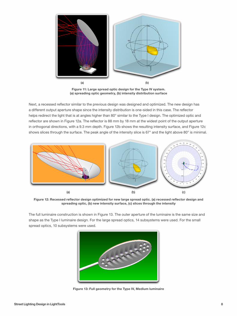
Figure 11: Large spread optic design for the Type IV system. (a) spreading optic geometry, (b) intensity distribution surface

Next, a recessed reflector similar to the previous design was designed and optimized. The new design has

a different output aperture shape since the intensity distribution is one-sided in this case. The reflector

helps redirect the light that is at angles higher than 80° similar to the Type I design. The optimized optic and

reflector are shown in Figure 12a. The reflector is 88 mm by 18 mm at the widest point of the output aperture

in orthogonal directions, with a 9.3 mm depth. Figure 12b shows the resulting intensity surface, and Figure 12c

shows slices through the surface. The peak angle of the intensity slice is 67° and the light above 80° is minimal.

Figure 12: Recessed reflector design optimized for new large spread optic. (a) recessed reflector design and spreading optic, (b) new intensity surface, (c) slices through the intensity

The full luminaire construction is shown in Figure 13. The outer aperture of the luminaire is the same size and

shape as the Type I luminaire design. For the large spread optics, 14 subsystems were used. For the small

spread optics, 10 subsystems were used.

Figure 13: Full geometry for the Type IV, Medium luminaire

(a) (b)

(a) (b) (c)


For this design, it was necessary to increase the power for the LEDs to meet the specification. All 24 LEDs

used for this design were calibrated to 220 lumens, which is mid range of the output flux shown in the LED

specifications. SLU was used to optimize the configuration of the lamps and a passing solution was found

using a mounting height of 8.6 meters and an overhang of 2.7 meters from the edge of the roadway. Since

the roadway is 20 meters long, the lamp spacing is 2.3 mounting heights, which is reasonable since the peak

intensity intersects the roadway at about 2.7 mounting heights for this lamp. Figure 14a shows the passing

specification items, and Figure 14b shows the mounting height plot, which indicates that the lamp is Type IV,

Medium. Figure 14c shows the intensity distribution surface for the full luminaire.

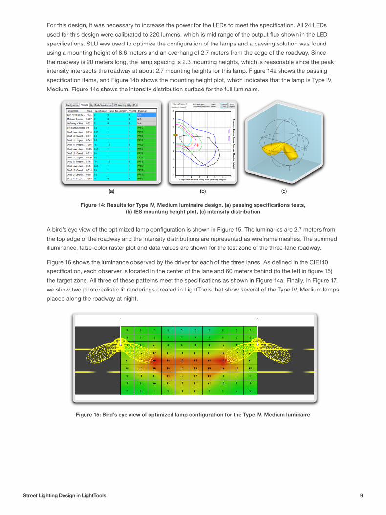
Figure 14: Results for Type IV, Medium luminaire design. (a) passing specifications tests, (b) IES mounting height plot, (c) intensity distribution

A bird’s eye view of the optimized lamp configuration is shown in Figure 15. The luminaries are 2.7 meters from

the top edge of the roadway and the intensity distributions are represented as wireframe meshes. The summed

illuminance, false-color raster plot and data values are shown for the test zone of the three-lane roadway.

Figure 16 shows the luminance observed by the driver for each of the three lanes. As defined in the CIE140

specification, each observer is located in the center of the lane and 60 meters behind (to the left in figure 15)

the target zone. All three of these patterns meet the specifications as shown in Figure 14a. Finally, in Figure 17,

we show two photorealistic lit renderings created in LightTools that show several of the Type IV, Medium lamps

placed along the roadway at night.

Figure 15: Bird’s eye view of optimized lamp configuration for the Type IV, Medium luminaire

(a) (b) (c)

Synopsys, Inc. 700 East Middlefield Road Mountain View, CA 94043 www.synopsys.com

©2012 Synopsys, Inc. All rights reserved. Synopsys is a trademark of Synopsys, Inc. in the United States and other countries. A list of Synopsys trademarks is available at http://www.synopsys.com/copyright.html. All other names mentioned herein are trademarks or registered trademarks of their respective owners.

06/12.AP.CS1725.

Figure 16: Luminance seen by the driver in each lane. (a) bottom lane (b) middle lane (c) top lane

SummaryIn this paper, we used LightTools and the Street Lighting Utility (SLU) to design and optimize two types

of solid state street lamps: Type I, Medium and Type IV, Medium. In addition to designing lamp geometry,

we used SLU to optimize the lamp configuration and power for the lamp sub-systems in order to pass the

specifications for a ME4a class roadway. LightTools quickly showed us the intensity surface distributions

and slices as well as allowing flexible optical surface parameterizations. SLU also let us analyze the

street configuration quickly and visualize the summed illuminance, luminance for each observer, and IES

classification of the lamps.

Figure 17: LightTools night-time photorealistic renderings of a scene with a roadway and several of the Type IV Medium lit lamps

(a) (b) (c)

http://www.synopsys.com/copyright.html