Elastic beams

Government Engineering College, Bhavnagar.

Civil Engineering Department

Advanced Engineering Mathematics

Topic:-Application of Ordinary Differential Equation

Elastic Beams.

Content

Beams

Elasticity

Application of Beams

Ordinary Differential Equations

Methods to Solve Ordinary Differential Equation

Euler–Bernoulli beam theory

Static beam equation

Derivation of bending moment equation

Assumptions of Classical Beam Theory

Second Order Method For Beam Deflections

What we learned?

Beams

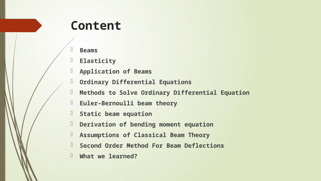
Beams are the most common type of structural component, particularly in Civil Engineering. Its length is comparatively more than its cross sectional area.

A beam is a bar like structural member whose primary function is to support transverse loading and carry it to the supports. See Figure.

A beam resists transverse loads mainly through bending action, Bending produces compressive longitudinal stresses in one side of the beam and tensile stresses in the other.

Elasticity

It is the property of the material to regain its original shape after the removal of external force.

As per the Hooke’s Law:-

“ Stress is directly proportional to the strain.”

i.e.

,

= E ,

Therefore we have,

E = /. ( Where , E = Young’s Modulus of Elasticity,

= Stress.

= Strain. )

Application of Beams

They are used as structural members in a structure. They transfer load from the superstructure to the

columns and to the sub-soil foundation. They are used in bridges for the transportation of light

as well as heavy vehicles. They are also as a strap beam in strap footing in

foundations to connect and transfer loads from the columns.

Ordinary Differential Equations

The Differential equation containing a single independent variable and the derivative with respect to it is called Ordinary Differential Equation.

Example:-

dy/dx = cx

dV/dx + q = 0

2x2 y’’ + x (2x + 1) y’ − y = 0.

Methods to Solve Ordinary Differential Equation

Variable Separable Method

Homogeneous and Non - Homogeneous Differential Equation Method

Exact and Non-exact Differential Equation Method

Linear and Non- Linear Differential Equation Method

Able’s Formula to find second solution of a Differential Equation

Wronskian method

Methods to find Complementary Function and Particular Integral of a Differential Equation.


Euler–Bernoulli beam theory (also known as engineer's beam theory or classical beam theory) is a simplification of the linear theory of elasticity which provides a means of calculating the load-carrying and deflection characteristics of beams.

It covers the case for small deflections of a beam that is subjected to lateral loads only. It is thus a special case of Timoshenko beam theory that accounts for shear deformation and is applicable for thick beams.

It was first enunciated circa 1750, but was not applied on a large scale until the development of the Eiffel Tower and the Ferris wheel in the late 19th century. Following these successful demonstrations, it quickly became a cornerstone of engineering and an enabler of the Second Industrial Revolution.

The Euler-Bernoulli beam equation is a combination of four different subsets of beam theory. These being the Kinematics

Constitutive

Force resultant

Equilibrium theories


Kinematics

Kinematics describes the motion of the beam and its deflection.

Kirchoff’s Assumptions The normal remain straight

The normal remain unstretched.

The normal remain to the normal (they are always perpendicular to the neutral plane)

Constitutive

The next equation needed to explain the Euler-Bernoulli equation is the constitutive equation.

Constitutive equations relate two physical quantities and in the case of beam theory the relation between the direct stress s and direct strain e within a beam is being investigated.

Force Resultant

These force resultants allow us to study the important stresses within the beam.

They are useful to us as they are only considered functions of, whereas the stresses found in a beam are functions.

Consider a beam cut at a point It is possible to find the direct stress and shear stress, and respectively, of that point. This is due to the direct stress at the cut producing a moment around the neutral plane. By summing all these individual moments over the whole of the cross-section it is possible to find the moment resultant M

Equilibrium

To keep things simple it is sufficient to deal with the stresses resultants rather than the stresses themselves.

The reason, explained previously, is that the resultants are functions of only.

The equilibrium equations are used to describe how the internal stresses of the beam are affected by the external loads being applied.


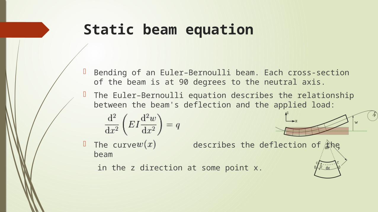
Bending of an Euler–Bernoulli beam. Each cross-section of the beam is at 90 degrees to the neutral axis.

The Euler–Bernoulli equation describes the relationship between the beam's deflection and the applied load:

The curve describes the deflection of the beam

in the z direction at some point x.

http://en.wikipedia.org/wiki/File:Euler-Bernoulli_beam_theory-2.svg


Continued…

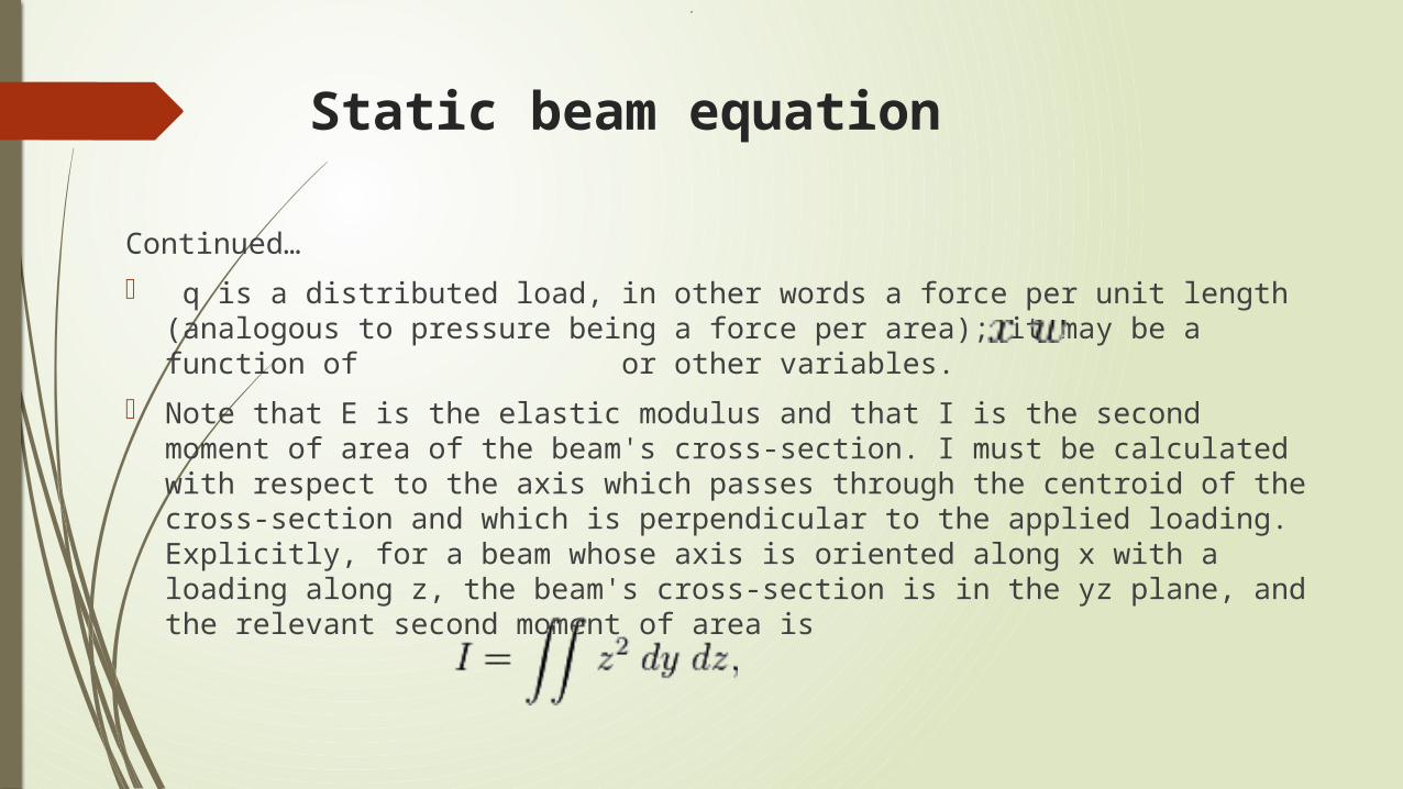
q is a distributed load, in other words a force per unit length (analogous to pressure being a force per area); it may be a function of or other variables.

Note that E is the elastic modulus and that I is the second moment of area of the beam's cross-section. I must be calculated with respect to the axis which passes through the centroid of the cross-section and which is perpendicular to the applied loading. Explicitly, for a beam whose axis is oriented along x with a loading along z, the beam's cross-section is in the yz plane, and the relevant second moment of area is

,


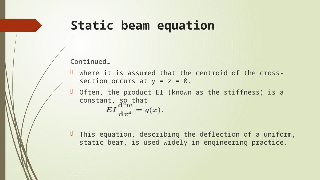
Continued…

where it is assumed that the centroid of the cross-section occurs at y = z = 0.

Often, the product EI (known as the stiffness) is a constant, so that

This equation, describing the deflection of a uniform, static beam, is used widely in engineering practice.


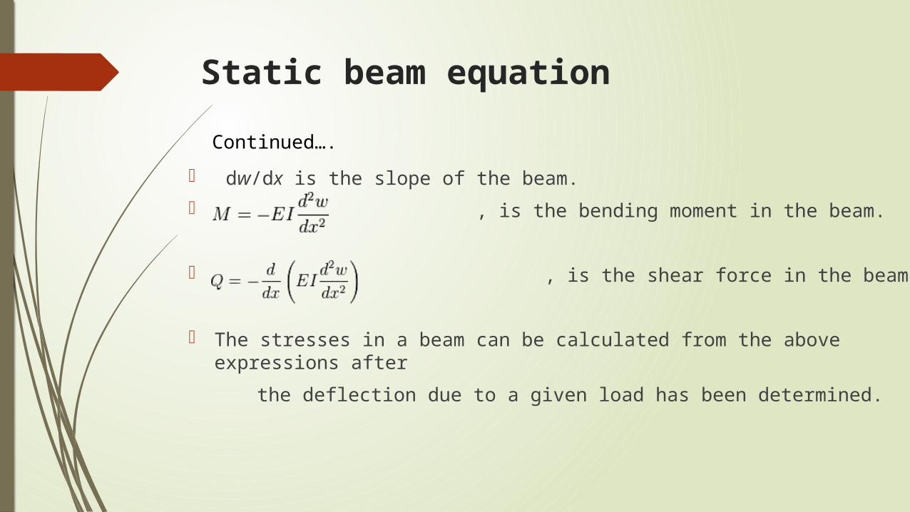
dw/dx is the slope of the beam.

, is the bending moment in the beam.

, is the shear force in the beam.

The stresses in a beam can be calculated from the above expressions after

the deflection due to a given load has been determined.

Continued….


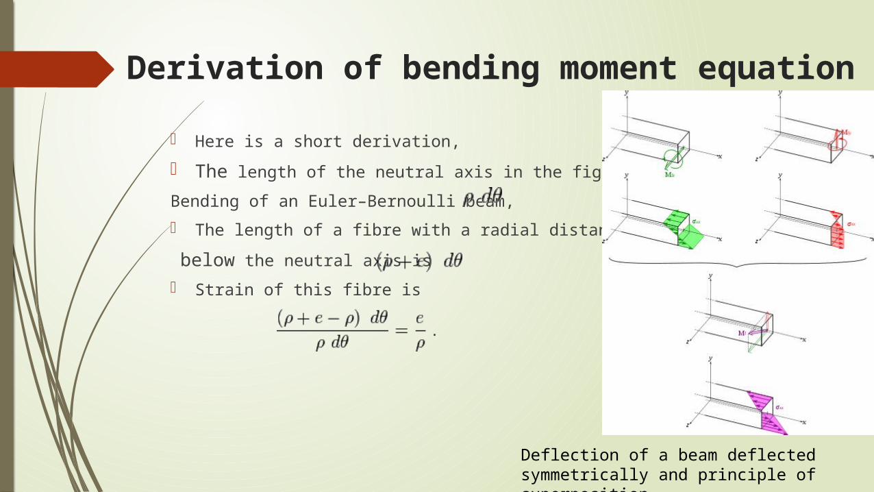
Here is a short derivation,

The length of the neutral axis in the figure,

Bending of an Euler–Bernoulli beam, .

The length of a fibre with a radial distance, e,

below the neutral axis is .

Strain of this fibre is

Deflection of a beam deflected symmetrically and principle of superposition


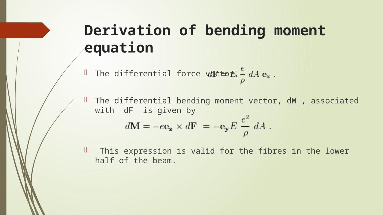
The differential force vector,

The differential bending moment vector, dM , associated with dF is given by

This expression is valid for the fibres in the lower half of the beam.


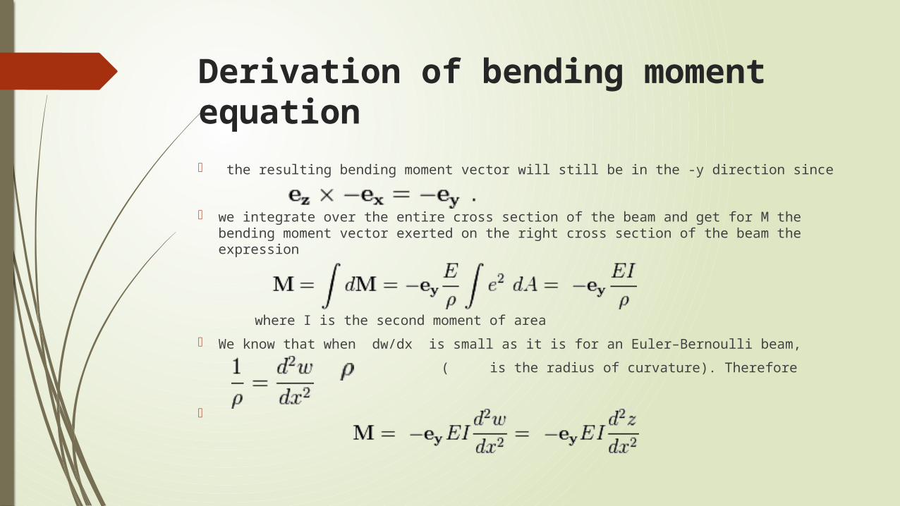
the resulting bending moment vector will still be in the -y direction since

we integrate over the entire cross section of the beam and get for M the bending moment vector exerted on the right cross section of the beam the expression

where I is the second moment of area

We know that when dw/dx is small as it is for an Euler–Bernoulli beam,

( is the radius of curvature). Therefore


1. Planar symmetry. The longitudinal axis is straight and the cross section of the beam has a longitudinal plane of symmetry. The resultant of the transverse loads acting on each section lies on that plane. The support conditions are also symmetric about this plane.

2. Cross section variation. The cross section is either constant or varies smoothly.

3. Normality. Plane sections originally normal to the longitudinal axis of the beam remain plane and normal to the deformed longitudinal axis upon bending.


4. Strain energy. The internal strain energy of the member accounts only for bending moment deformations. All other contributions, notably transverse shear and axial force, are ignored.

5. Linearization. Transverse deflections, rotations and deformations are considered so small that the assumptions of infinitesimal deformations apply.

6. Material model. The material is assumed to be elastic and isotropic. Heterogeneous beams fabricated with several isotropic materials, such as reinforced concrete, are not excluded.

Second Order Method For Beam Deflections

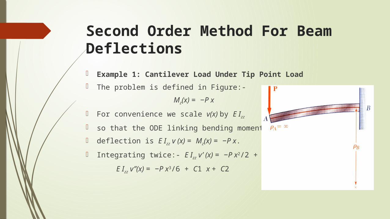
Example 1: Cantilever Load Under Tip Point Load

The problem is defined in Figure:-

Mz(x) = −P x

For convenience we scale v(x) by E Izz

so that the ODE linking bending moment to

deflection is E Izz v (x) = Mz(x) = −P x.

Integrating twice:- E Izz v’ (x) = −P x2/2 + C1

E Izz v’’(x) = −P x3/6 + C1 x + C2

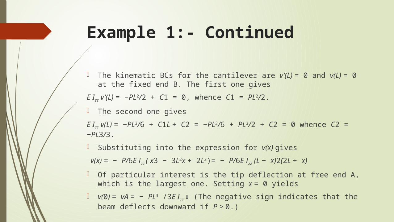
Example 1:- Continued

The kinematic BCs for the cantilever are v’(L) = 0 and v(L) = 0 at the fixed end B. The first one gives

E Izz v’(L) = −PL2/2 + C1 = 0, whence C1 = PL2/2.

The second one gives

E Izz v(L) = −PL3/6 + C1L + C2 = −PL3/6 + PL3/2 + C2 = 0 whence C2 = −PL3/3.

Substituting into the expression for v(x) gives

v(x) = − P/6E Izz ( x3 − 3L2x + 2L3)= − P/6E Izz (L − x)2(2L + x)

Of particular interest is the tip deflection at free end A, which is the largest one. Setting x = 0 yields

v(0) = vA = − PL3 /3E Izz ⇓ (The negative sign indicates that the beam deflects downward if P > 0.)

What we learned?

Total amount of deflection which will occur. Merits and Demerits of this theory. Comparison Between the two theories.

(Timoshenko Beam Theory and Euler–Bernoulli beam theory.)

Frequency of a Vibrating System Using a Vertical beam.

Thank You For Bearing.

By, Nitin Charel (130210106011) Kartik Hingol (130210106030) Bhavik Shah (130210106049) Yash Shah (130210106052) Digvijay Solanki (130210106055)