Professor Terje Haukaas University of British Columbia, Vancouver www.inrisk.ubc.ca

2D Elastic Beams Updated February 21, 2014 Page 1

2D Elastic Beams In other documents on this website, the Euler-Bernoulli and Timoshenko beam theories are described. Both those theories are based on the assumption that “plane sections remain plane.” That is not an exact description of reality and this document describes an alternative, based on the 2D theory of elasticity. In particular, a cantilevered beam in the x-z-plane is considered in the following, as shown in Figure 1. In another document on 2D elasticity theory, the 4th-order differential equation for the stress function is derived. Written in terms of x and z it reads

∂4 F∂x4 + ∂4 F

∂z4 + ∂4 F∂x2 ∂z2 = 0 (1)

Figure 1: Beam on elastic foundation.

The solution for specific problems is established by formulating a stress function that satisfies the unique boundary conditions for each problem. As a demonstration, the cantilever in Figure 1 is considered in this section. To simplify the mathematical expressions, the fixed support is on the right-hand side and the load is applied on the left-hand side. A solution for this problem, where the horizontal edges are stress-free and the edge at x=0 has a shear stress resultant P, is obtained by combining the stress function for pure shear and a stress function with a 3rd-order term (Timoshenko and Goodier 1969):

F(x, z) = C1 ⋅ x ⋅ z +C2 ⋅ x ⋅ z3 (2)

This stress function yields the following stresses:

σ xx =

∂2 F∂z2 = 6 ⋅C2 ⋅ x ⋅ z (3)

σ zz =

∂2 F∂x2 = 0 (4)

x

z

P

L

h

Professor Terje Haukaas University of British Columbia, Vancouver www.inrisk.ubc.ca

2D Elastic Beams Updated February 21, 2014 Page 2

τ xz = − ∂2 F

∂x∂z= −C1 − 3⋅C2 ⋅ z

2 (5)

Zero stress on the horizontal edges implies that

τ xz (z = ± h

2 ) = −C1 − 3⋅C2 ⋅h2

⎛⎝⎜

⎞⎠⎟

2

= 0 ⇒ C2 = − 43h2 ⋅C1 (6)

Shear stress resultant P at x=0 implies that

τ xz (x = 0)dz− h

2

h2

∫ = −C1 − 3⋅C2 ⋅ z2 dz

− h2

h2

∫ = − 2h3

C1 = −P ⇒ C1 =3P2h

(7)

which implies that

C2 = − 4

3⋅h2 ⋅3P2h

= − 2Ph3 (8)

Substitution of C1 and C2 into Eq. (3) yields the axial stress

σ xx = 6 ⋅C2 ⋅ x ⋅ z = −12P

h3 ⋅ x ⋅ z = − PI⋅ x ⋅ z (9)

where I=h3/12 is introduced for this unit-width beam to echo the notation in elementary beam theory. In fact, the axial stress is distributed exactly as in elementary beam theory. Substitution of C1 and C2 into Eq. (5) yields the shear stress

τ xz = −C1 − 3⋅C2 ⋅ z

2 = − 3P2h

+ 6Ph3 z2 = − 3P

2h1− 2z

h⎛⎝⎜

⎞⎠⎟

2⎛

⎝⎜

⎞

⎠⎟ (10)

where it is observed again that the solution is exactly as in the elementary beam theory, assuming that the load P is applied on the edge distributed according to the parabola in Eq. (10). However, more information is available from this elasticity solution than beam theory. In particular, displacements can be calculated, and these reveal that plane sections do not remain plane during bending. To see this, i.e., to compute the displacements associated with the stresses above, the general kinematics equations are invoked, which read

ε xx =

∂u∂x

(11)

ε zz =

∂w∂z

(12)

γ xz =

∂u∂z

+ ∂w∂x

(13)

The material law is also needed, which for plane stress (thin beam in the y-direction) read

Professor Terje Haukaas University of British Columbia, Vancouver www.inrisk.ubc.ca

2D Elastic Beams Updated February 21, 2014 Page 3

ε xx =

1E⋅ σ xx −ν ⋅σ zz( ) (14)

ε zz =

1E⋅ σ zz −ν ⋅σ xx( ) (15)

γ xz =

τ xz

G (16)

where G=E(2(1+ν)) is the shear modulus. The material law for plane strain (infinitely thick beam in the y-direction) is obtained by replacing E by E/(1–ν2) and ν by ν/(1–ν) (Timoshenko and Goodier 1969), which yields

ε xx =

1E⋅ (1−ν 2 ) ⋅σ xx −ν ⋅(1+ν ) ⋅σ zz( ) (17)

ε zz =

1E⋅ (1−ν 2 ) ⋅σ zz −ν ⋅(1+ν ) ⋅σ xx( ) (18)

γ xz =

τ xz

G (19)

For the plane stress case, the combination of the kinematics equations (11) to (13) with the material law equations (14) to (16), and substitution of stresses from Eqs. (9) and (10) together with σzz=0 yields

ε xx =

∂u∂x

= 1E⋅ σ xx −ν ⋅σ zz( ) = σ xx

E= − P

EI⋅ x ⋅ z (20)

ε zz =

∂w∂z

= 1E⋅ σ zz −ν ⋅σ xx( ) = − 1

E⋅ν ⋅σ xx =

PEI

⋅ν ⋅ x ⋅ z (21)

γ xz =

∂u∂z

+ ∂w∂x

=τ xz

G= − 3P

2Gh1− 2z

h⎛⎝⎜

⎞⎠⎟

2⎛

⎝⎜

⎞

⎠⎟ (22)

Integration of Eqs. (20) and (21) yields the general displacement expressions

u(x, z) = − P

EI⋅ x ⋅ z dx∫ = − Pzx2

2EI+ hz (z) (23)

w(x, z) = P

EI⋅ν ⋅ x ⋅ z dz∫ = Pνxz2

2EI+ hx (x) (24)

where hx(x) and hz(z) are functions that represent the integration constants. Substitution of Eqs. (23) and (24) into Eq. (22) yields

∂u∂z

+ ∂w∂x

= − Px2

2EI+∂hz (z)∂z

+ Pν z2

2EI+∂hx (x)∂x

= − 3P2Gh

1− 2zh

⎛⎝⎜

⎞⎠⎟

2⎛

⎝⎜

⎞

⎠⎟ (25)

Professor Terje Haukaas University of British Columbia, Vancouver www.inrisk.ubc.ca

2D Elastic Beams Updated February 21, 2014 Page 4

By separating terms that depend on x and z, the following reorganized equation is obtained:

− Px2

2EI+∂hx (x)∂x

F ( x )! "## $##

+ Pν z2

2EI+∂hz (z)∂z

− 6Pz2

Gh3

G( z )! "### $###

= − 3P2Gh

K!"$

(26)

where F(x), G(z), and K are defined so that Eq. (25) can be written (Timoshenko and Goodier 1969) F(x)+G(z) = K (27)

Because the right-hand side is constant, F(x) and G(z) must also be constants, here named C3 and C4:

F(x) = − Px2

2EI+∂hx (x)∂x

= C3 ⇒ ∂hx (x)∂x

= Px2

2EI+C3 (28)

G(z) = Pν z2

2EI+∂hz (z)∂z

− 6Pz2

Gh3 = C4 ⇒ ∂hz (z)∂z

= 6Pz2

Gh3 − Pν z2

2EI+C4 (29)

Integration yields hx(x) and hz(z) expressed in terms of unknown constants:

hx (x) = Px2

2EI+C3

⎛⎝⎜

⎞⎠⎟

dx∫ = Px3

6EI+C3x +C5 (30)

hz (z) = 6Pz2

Gh3 − Pν z2

2EI+C4

⎛⎝⎜

⎞⎠⎟

dz∫ = 2Pz3

Gh3 − Pν z3

6EI+C4z +C6 (31)

Substitution of the functions hx(x) and hz(z) in Eqs. (30) and (31) into the displacements in Eqs. (23) and (24) yields

u(x, z) = − Pzx2

2EI+ 2Pz3

Gh3 − Pν z3

6EI+C4z +C6 (32)

w(x, z) = Pνxz2

2EI+ Px3

6EI+C3x +C5 (33)

The constants C3, C4, C5, and C6 are determined from Eq. (27), which says that

C3 +C4 = − 3P

2Gh (34)

and from three boundary conditions that prevent the beam from displacing as a rigid body. For the beam in Figure 1, it is natural to enforce zero displacements and zero rotation at the point where x=L and z=0. According to Eqs. (32) and (33), zero displacement implies that

u(L,0) = C6 = 0 (35)

Professor Terje Haukaas University of British Columbia, Vancouver www.inrisk.ubc.ca

2D Elastic Beams Updated February 21, 2014 Page 5

w(L,0) = PL3

6EI+C3L+C5 = 0 (36)

Interestingly, the zero-rotation-requirement can be imposed in several ways because plane sections do not remain plane and perpendicular to the neutral axis. One option is to require that a vertical line remains vertical:

∂u(L,0)

∂z= − PL2

2EI+C4 = 0 ⇒ C4 =

PL2

2EI (37)

Eq. (34) then yields

C3 = − 3P

2Gh− PL2

2EI (38)

Eq. (36) then yields

C5 = − PL3

6EI+ 3PL

2Gh+ PL3

2EI= PL3

3EI+ 3PL

2Gh (39)

which means that all the constants C3, C4, C5, and C6 are determined and the final displacement expressions are:

u(x, z) = − Pzx2

2EI+ 2Pz3

Gh3 − Pν z3

6EI+ PL2

2EI⋅ z (40)

w(x, z) = Pνxz2

2EI+ Px3

6EI+ − 3P

2Gh− PL2

2EI⎛⎝⎜

⎞⎠⎟

x + PL3

3EI+ 3PL

2Gh (41)

Another option for enforcing zero rotation at the end is the classical requirement that a horizontal line remains horizontal:

∂w(L,0)∂x

= PL2

2EI+C3 = 0 ⇒ C3 = − PL2

2EI (42)

Eq. (34) then yields

C4 =

PL2

2EI− 3P

2Gh (43)

Eq. (36) then yields

C5 = − PL3

6EI+ PL3

2EI= PL3

3EI (44)

which means that all the constants C3, C4, C5, and C6 are determined and the final displacement expressions are:

u(x, z) = − Pzx2

2EI+ 2Pz3

Gh3 − Pν z3

6EI+ PL2

2EI− 3P

2Gh⎛⎝⎜

⎞⎠⎟

z (45)

Professor Terje Haukaas University of British Columbia, Vancouver www.inrisk.ubc.ca

2D Elastic Beams Updated February 21, 2014 Page 6

w(x, z) = Pνxz2

2EI+ Px3

6EI− PL2

2EIx + PL3

3EI (46)

It is interesting to note that the tip-deflection of the cantilever equals the classical result PL3/3EI for Eq. (46) while for the solution in Eq. (41) it is

w(x, z) = PL3

3EI+ 3PL

2Gh (47)

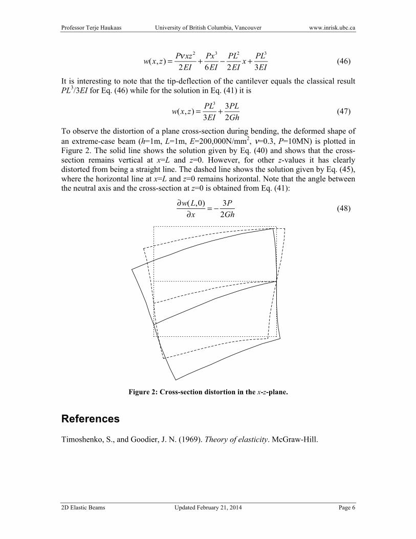
To observe the distortion of a plane cross-section during bending, the deformed shape of an extreme-case beam (h=1m, L=1m, E=200,000N/mm2, ν=0.3, P=10MN) is plotted in Figure 2. The solid line shows the solution given by Eq. (40) and shows that the cross-section remains vertical at x=L and z=0. However, for other z-values it has clearly distorted from being a straight line. The dashed line shows the solution given by Eq. (45), where the horizontal line at x=L and z=0 remains horizontal. Note that the angle between the neutral axis and the cross-section at z=0 is obtained from Eq. (41):

∂w(L,0)∂x

= − 3P2Gh

(48)

Figure 2: Cross-section distortion in the x-z-plane.

References

Timoshenko, S., and Goodier, J. N. (1969). Theory of elasticity. McGraw-Hill.