2

Stress-Strain Analysis of a Cylindrical Pipe Subjected to a Transverse

Load and Large Deflections

R.M. Guedes

INEGI - Mecânica Experimental e Novos Materiais, Faculdade de Engenharia,

Universidade do Porto, Rua Dr. Roberto Frias s/n, 4200-465 Porto, Portugal

ABSTRACT

The increased use of polymers and reinforced polymers in civil construction

applications originated elegant structures with a high specific strength and stiffness. The

mechanical performance improved significantly in comparison with traditional

materials; however the structural engineers face new challenges. The high strength

compared with the stiffness of these new materials allows large deformations without

failure or damage, especially in large structures. The classical theories, i. e. based on

small deformations, became no longer valid and corrections must be used. The aim of

this work was to show this occurrence in a practical case, used in civil engineering

construction. For that purpose a glass-fiber reinforced (GRP) buried pipe under a

transverse load was analyzed. Strains experimentally measured and FEM analyses are

used to verify the phenomenon. In this case the relation between the maximum

3

deflection and the maximum hoop strain was no longer linear as predicted by the small

deformation theory. A simple approach using deformation components based on finite

deformations theory was proposed and assessed. Although this approach, which has an

analytical integral solution, does not predict accurately the nonlinear phenomena it

allowed a dimensionless parametric study of the problem. A simple correction of this

approach is proposed and assessed.

KEYWORDS: Polymer-matrix composites (PMCs); Non-linear behaviour; Finite

element analysis (FEA); Elasticity; Finite Deformations.

INTRODUCTION

The use of composite materials for piping systems and other civil engineering structures

has renewed interest in problems of stress analysis of cylindrical composite structures.

Standard methodologies, for mechanical characterization of plastic piping systems,

subject ring pipes to a specified diametric compressive loading. In the present case the

pipe sections had an internal diameter of 500 mm and an external diameter of about 524

mm, i.e. a wall thickness of about 12 mm. The nominal ring circumferential stiffness

was 10.5 GPa and the circumferential strength close to 250 MPa. Usually these

structures are considered thin rings and the classical theories, based on small

displacements, provide an accurate solution for these cases. However when high

strength is combined with relative low stiffness, large deformations take place before

failure occurs.

4

This phenomenon is analysed using Finite Element Analysis and experimental data. The

relationship between maximum hoop strain and maximum deflection is no longer linear

as predicted by small displacement theory. An analytical integral solution using

deformation components based on finite deformations theory is presented and assessed.

As far our knowledge goes, there are no analytical integral solutions for the specific

problem described. In this type of problems the solution is given in terms of elliptical

integrals, which have to be numerically integrated [1]. Furthermore few works call the

attention for the geometrical nonlinear effects which can occur in composite structures.

This is especially critical when measuring the mechanical properties until structural

collapse or failure is verified. Consequently the nonlinear geometrical phenomenon can

be mistaken for damage.

Tse et al. [2-4] engaged on a complete study of large deflection problem of circular

springs under uniaxial load (tension and compression). The solutions were obtained in

terms of elliptical integrals. Comparisons with experimental data show a good

agreement between theoretical approach and experimental results.

Sheinman [5] proposed a general analytical and numerical procedure, based on large

deflections, small strains and moderately small rotations, for an arbitrary plane curved

beam made of linear elastic. The influence of shear stiffness was also considered.

Several papers analysed large displacements of plane and curved cantilever beams. The

classical problem of the deflection of a cantilever beam of linear elastic material, under

the action of an external vertical concentrated load at the free end, was analysed

considering large deflections [6]. As the authors mention the mathematical treatment of

the equilibrium of cantilever beams does not involve a great degree of difficulty

however analytical solution does not exist. Carrillo [7] analysed the deflections of a

5

cantilevered beam made of a linear-elastic material under the influence of a vertical

concentrated force at the free end. The author shows that the widely known simple

solution for small deflections is a limiting case, which holds when forces applied are

much smaller than the allowable maximum force before beam failure. González and

LLorca [8] studied the deformation of an inextensible, curved elastic beam subjected to

axial load by including the effect of large displacements. The load–axial displacement

curves were accurately fitted to a polynomial expression which provided the evolution

of the beam stiffness during deformation.

CURVED BEAM THEORY FOR SMALL DEFLECTIONS (CBTSD):

CLASSICAL SOLUTION

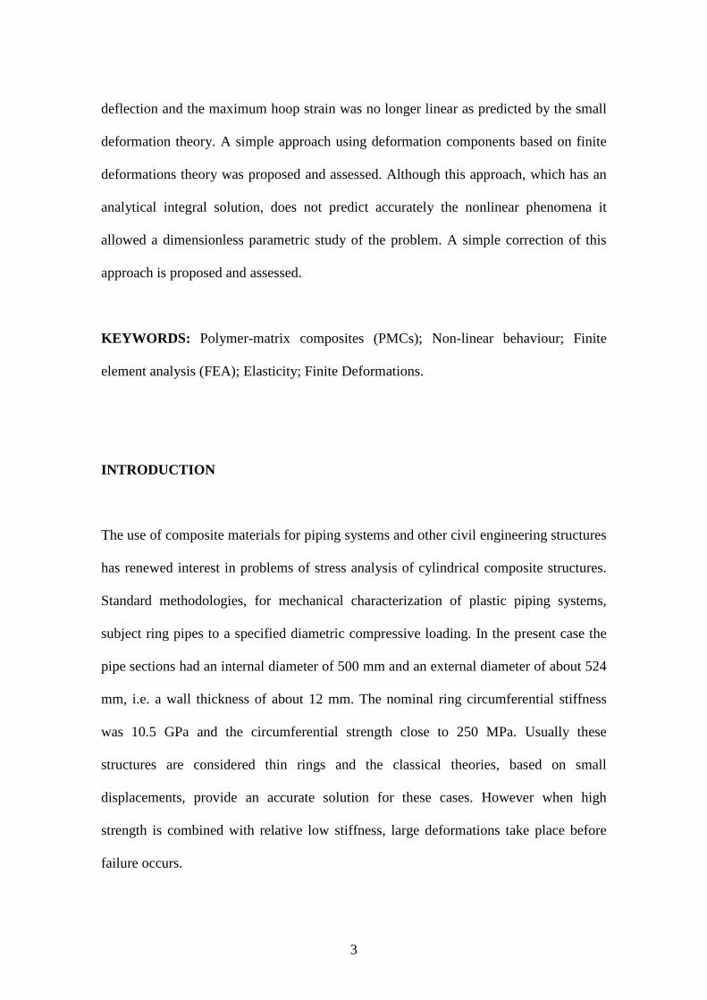
In Figure 1 is depicted the half-view of the pipe along with the general geometrical

parameters, where R represents the middle plane radius.

O

R

V0=-F/2

M0 M0

V0 θ

w0(θ) u0(θ)

Figure 2- The half-view of the pipe.

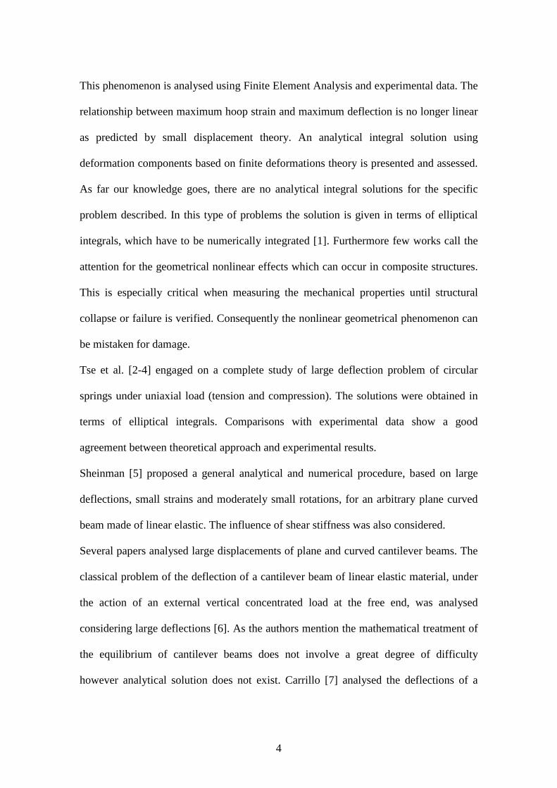
The differential equations of equilibrium [9-11], in polar coordinates, are

6

( ) ( )

( ) ( )

( ) ( )

0

0

0

N V

V N

M RV

θ θθ

θ θθ

θ θθ

∂ + =∂

∂ − =∂∂ − =∂

. (1)

Using the following boundary conditions,

( ) ( )( )( ) ( )

0

02

0

0 0

FV V

M M

N N

π

π

= = − = = =

. (2)

The system is readily solved,

( ) ( )( ) ( )( ) ( )

0

0

0 0

N V sin

V V cos

M M RV sen

θ θθ θθ θ

= −

= = +

. (3)

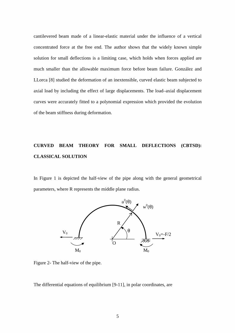
For thin beams the middle surface strain 0ε and curvature κ changes are:

00 0

2 0 0

2 2

1

1

uw

R

w u

R

εθ

κθ θ

∂= + ∂

∂ ∂ = − + ∂ ∂

. (5)

where 0u is the tangential displacement and 0w the radial displacement of the beam

middle surface.

The normal strain at an arbitrary point can be found using

( )01

1z

z Rε ε κ= +

+. (7)

7

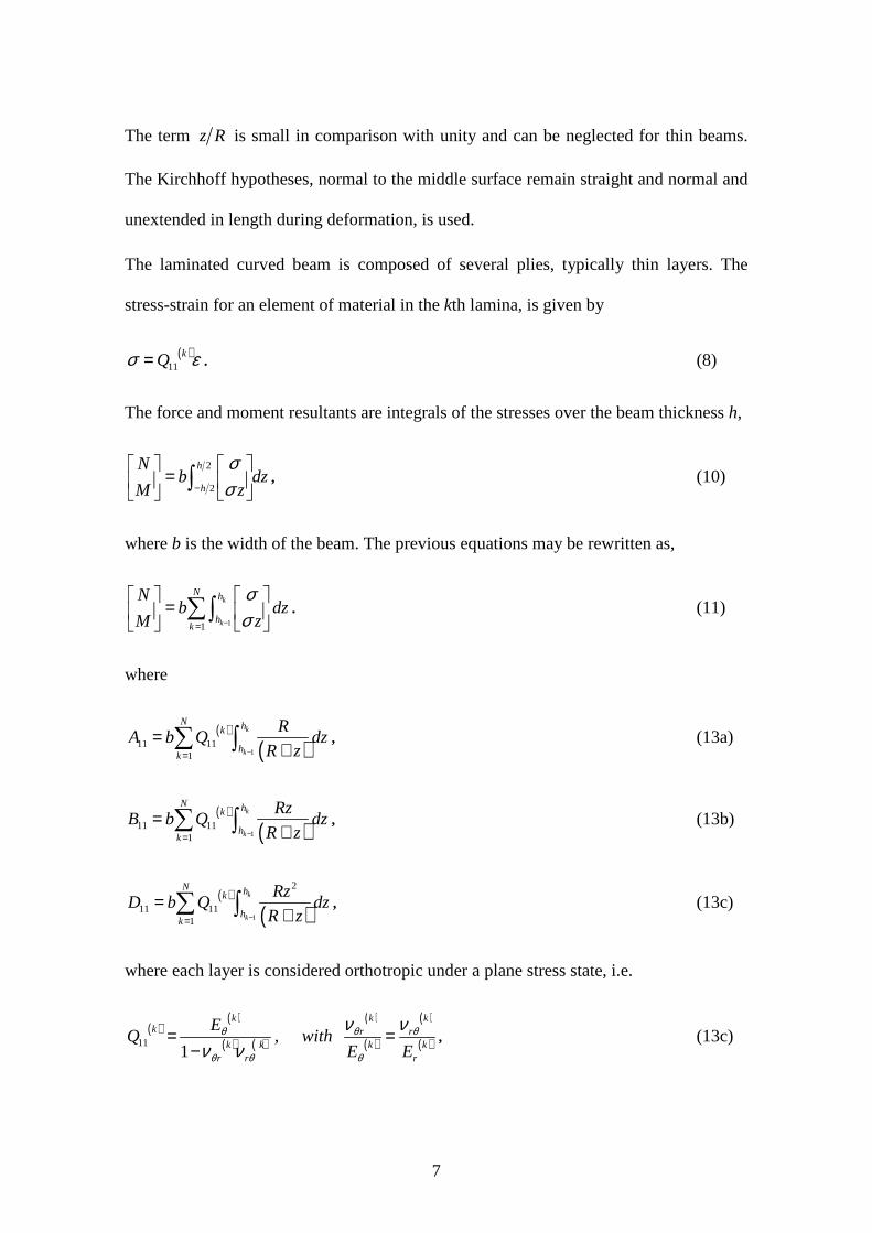
The term z R is small in comparison with unity and can be neglected for thin beams.

The Kirchhoff hypotheses, normal to the middle surface remain straight and normal and

unextended in length during deformation, is used.

The laminated curved beam is composed of several plies, typically thin layers. The

stress-strain for an element of material in the kth lamina, is given by

( )11

kQσ ε= . (8)

The force and moment resultants are integrals of the stresses over the beam thickness h,

2

2

h

h

Nb dz

M z

σσ−

=

∫ , (10)

where b is the width of the beam. The previous equations may be rewritten as,

11

k

k

N h

hk

Nb dz

M z

σσ−=

=

∑∫ . (11)

where

( )

( )111 11

1

k

k

N hk

hk

RA b Q dz

R z−==

+∑ ∫ , (13a)

( )

( )111 11

1

k

k

N hk

hk

RzB b Q dz

R z−==

+∑ ∫ , (13b)

( )

( )1

2

11 111

k

k

N hk

hk

RzD b Q dz

R z−=

=+∑ ∫ , (13c)

where each layer is considered orthotropic under a plane stress state, i.e.

( )( )

( ) ( )

( )

( )

( )

( )111

k k kk r r

k k k kr r r

EQ , with

E Eθ θ θ

θ θ θ

ν νν ν

= =−

, (13c)

8

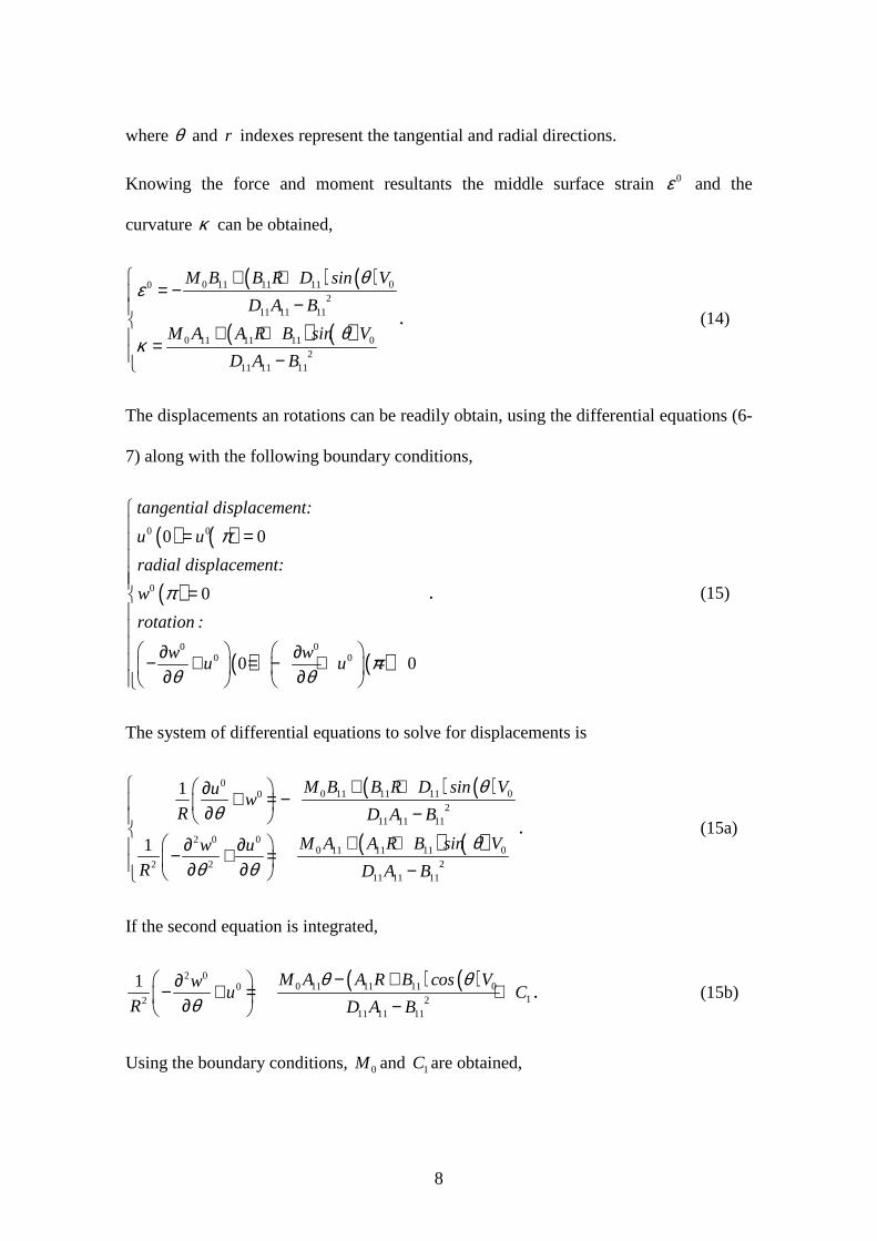
where θ and r indexes represent the tangential and radial directions.

Knowing the force and moment resultants the middle surface strain 0ε and the

curvature κ can be obtained,

( ) ( )

( ) ( )

0 11 11 11 002

11 11 11

0 11 11 11 02

11 11 11

M B B R D sin V

D A B

M A A R B sin V

D A B

θε

θκ

+ += − −

+ + =

−

. (14)

The displacements an rotations can be readily obtain, using the differential equations (6-

7) along with the following boundary conditions,

( ) ( )

( )

( ) ( )

0 0

0

0 00 0

0 0

0

0 0

tangential displacement:

u u

radial displacement:

w

rotation :

w wu u

π

π

πθ θ

= = = ∂ ∂− + = − + = ∂ ∂

. (15)

The system of differential equations to solve for displacements is

( ) ( )

( ) ( )

00 11 11 11 00

211 11 11

2 0 00 11 11 11 0

22 211 11 11

1

1

M B B R D sin Vuw

R D A B

M A A R B sin Vw u

R D A B

θθ

θθ θ

+ + ∂ + = − ∂ −

+ + ∂ ∂ − + = ∂ ∂ −

. (15a)

If the second equation is integrated,

( ) ( )2 00 11 11 11 00

12211 11 11

1 M A A R B cos Vwu C

R D A B

θ θθ

− + ∂− + = + ∂ − . (15b)

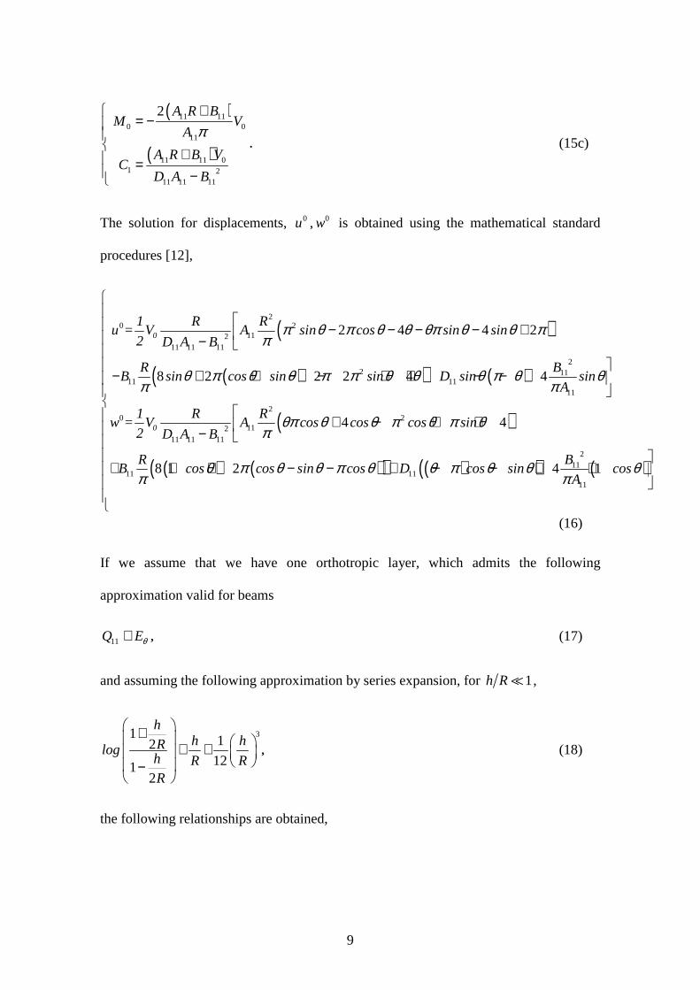
Using the boundary conditions, 0M and 1C are obtained,

9

( )

( )

11 110 0

11

11 11 01 2

11 11 11

2 A R B M V

A

A R B VC

D A B

π+

= − + = −

. (15c)

The solution for displacements, 0u , 0w is obtained using the mathematical standard

procedures [12],

( )

( )( ) ( )

( )

( )

20 2

11211 11 11

22 11

11 1111

20 2

11211 11 11

11

2 4 4 2

8 2 2 2 4 4

4 4

8 1 2

0

0

1 R Ru = V A sin cos sin sin

2 D A B

R BB sin cos sin sin D sin sin

A

1 R Rw = V A cos cos cos sin

2 D A B

RB cos cos

π θ π θ θ θπ θ θ ππ

θ π θ θ π π θ θ θ π θ θπ π

θπ θ θ π θ π θπ

θ π θπ

− − − − +−

− + + − − + + − −

+ − + +−

+ + + ( )( ) ( )( ) ( )2

1111

11

4 1B

sin cos D cos sin cosA

θ π θ θ π θ θ θπ

− − + − − + + (16)

If we assume that we have one orthotropic layer, which admits the following

approximation valid for beams

11Q Eθ≅ , (17)

and assuming the following approximation by series expansion, for 1h R≪ ,

31 12121

2

hh hRlog

h R RR

+ ≅ + −

, (18)

the following relationships are obtained,

10

11

12

12

h

RA bE Rlog bE hh

R

θ θ

+ = ≅

−

, (19a)

32

11

12

1212

hbE hh RB bE R log

hR RR

θθ

+ = − ≅ −

−

, (19b)

33

11

12

1212

hbE hh RD bE R log

hRR

θθ

+ = − ≅

−

, (19c)

2

0 0

2

6

R hM V

Rπ π

= − −

. (19d)

The maximum moment is obtained for 0θ = , i.e. 0maxM M= . Concomitantly the

maximum radial deflection is obtained for 0θ = ,

( )( )( ) ( )

2 2 2

0 003

2 24 3 20 0 0

R R hw V , u

bE hθ

ππ− −

= = , (20a)

( ) ( )00 03

24 20 0

Rk V , V

bE h bE hθ θ

επ π

= = . (20b)

The maximum hoop strain, obtained from Equation (7), is given by

( )( )( ) 02

4 61 1

2max

h RV

E bR h R h Rθ

επ

±=

± ∓ . (21)

The maximum hoop strain depends linearly on the applied transverse load. Furthermore

the maximum hoop strain can be obtained as function of the maximum deflection

( )0 0w ,

11

( )0

22

2 60

2 3 24 2max

h hwR R

Rh h

R R

επ

± = ±

± − +

. (22)

This expression can be simplified, since 1h R≪ ,

( )( )0

2

2 0

8max

hwR

Rε

π≅ ±

−. (23)

This result coincides with result obtained for thin beam theory as it should be expected

[13]. In conclusion the maximum hoop strain depends only on the geometry and the

maximum radial displacement and it is linearly proportional to the maximum radial

displacement.

CURVED BEAM THEORY FOR LARGE DEFLECTIONS (CBTLD): AN

APPROXIMATE SOLUTION BASED ON FINITE DEFORMATIONS THEORY

Accordingly with Ambartsumyan [14] the theory of finite deformations, or the non-

linear theory of elasticity, differs significantly from the linear theory of elasticity due to

certain geometric properties contained within it. The fundamental difference is that the

theory of finite deformations takes into account the difference between the geometry of

the deformed and undeformed states. Based on finite deformations theory the hoop

strain [14] is given by

20 00 0 2 0

2

1 1 1

2 2

u uw w

R Rε ϕ

θ θ ∂ ∂= + + + + ∂ ∂

. (24)

12

Assuming 20

02

10

2

uw

R θ ∂ + ≈ ∂

the Equation (24) can be simplified,

00 0 21 1

2

uw

Rε ϕ

θ ∂= + + ∂

, (24a)

where

001 w

R uR

ϕ κ ϕθ θ

∂ ∂= → = − + ∂ ∂ . (25)

In order to have an analytical integral solution; it was not considered the influence of

geometry of the deformed state on the bending moment distribution. This is an

important drawback of the present approach. However if that was taken it account, the

problem could only be solved numerically (solution in terms of elliptical integrals), as it

was done previously by Tse et al. [2].

In this case the system of differential equations, for one orthotropic layer, to solve for

displacements and curvature is

( )( )( )( )

00 2 0

2 2

2 20 0

3 2 2

121 1

2 12

12 12 12

12

M Ruw

R bE h R h

R M R R h V sin

bE h R h

θ

θ

ϕθ

θκ

∂ + + = ∂ −

− −= −

. (26)

From the last equation ϕ can be calculated

( )( )23

0 033 2 2

12 1144

12

R cosRM V

bE hbE h R h θθ

θθϕ−

= −−

. (27)

Therefore the system of differential equations can be written as

13

( ) ( )( )

( )( )

220 3

0 00 032 2 3 2 2

20 30

0 033 2 2

12 1121 1 144

212 12

12 11 144

12

R cosM Ru Rw M V

R bE hbE h R h bE h R h

R cosw Ru M V

R bE hbE h R h

θθ θ

θθ

θθθ

θθθ

− ∂ + = − − ∂ − − − ∂− + = + ∂ −

.

(28)

The boundary conditions are, of course, the same as for the CBTSD. The general

solution is given in appendix. The solution for 0M is exactly the same that was obtained

for the CBTSD. For 0θ = the strain and curvature are the same, as obtained from the

CBTSD, but not the radial displacement,

( ) ( )( )

( )( )

2 2 25 220 0

0 02 33

2 3 24 22 576 600 0 0

R R hRw V V , u

bE hbE h θθ

ππππ

− +− = + = , (29)

( ) ( )00 03

24 20 0

Rk V , V

bE h bE hθ θ

επ π

= = . (30)

As before the strain can be obtained as function of the maximum deflection ( )0 0w ,

( )( )( )0

22

0

4 20

22 8 0

3

max

h hwR R

Rh hw

R R

επ ξ

± = ±

± − + +

, (31a)

where

( )( ) ( ) ( ) 2 422 2 2

0

040 4 31 40 8 128

3 3 3 3

w h hw

R R Rξ π π π = − + − + − +

. (31b)

This could be simplified, since 1h R≪ ,

14

( )( )( )( )0

20

4 0

8 0max

hwR

Rwε

π ξ≅ ±

− +, (32a)

where

( )( ) ( ) ( )22 20

01200 8 128

9

ww

Rξ π π ≅ − + −

. (32b)

Hence, as for the CBTSD solution, the maximum hoop strain depends only on the

geometry, i.e. the h/R ratio, and on the maximum radial displacement. However the

linear relationship, between maximum hoop strain and the maximum radial

displacement, no longer holds.

NON-LINEAR FEM SIMULATION

A 2D FEM modeling with a very refined mesh was used with 17110 CPE8R planar

elements of ABAQUSTM using a large displacement formulation. Two different cases

were simulated using the same ratio h/R=3/64, described in Table 1, to verify the

dimensionless relationships obtained using the CBTLD.

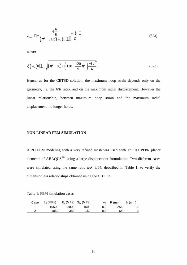
Table 1: FEM simulation cases

Case Eθ (MPa) Er (MPa) Gθr (MPa) νθr R (mm) h (mm)1 10500 3800 1500 0.3 256 122 1050 380 150 0.3 64 3

15

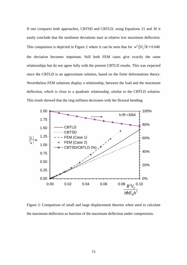
If one compares both approaches, CBTSD and CBTLD, using Equations 21 and 30 it

easily conclude that the nonlinear deviations start at relative low maximum deflection.

This comparison is depicted in Figure 2 where it can be seen that for ( )0 0 0 040w R .>

the deviation becomes important. Still both FEM cases give exactly the same

relationships but do not agree fully with the present CBTLD results. This was expected

since the CBTLD is an approximate solution, based on the finite deformations theory.

Nevertheless FEM solutions display a relationship, between the load and the maximum

deflection, which is close to a quadratic relationship, similar to the CBTLD solution.

This result showed that the ring stiffness decreases with the flexural bending.

0.00

0.25

0.50

0.75

1.00

1.25

1.50

1.75

2.00

0.00 0.02 0.04 0.06 0.08 0.10

0%

20%

40%

60%

80%

100%

CBTLDCBTSDFEM (Case 1)FEM (Case 2)CBTSD/CBTLD (%)

20

3

R V

bE hθπ

()

00

w

R

h /R =3/64

Figure 2: Comparison of small and large displacement theories when used to calculate

the maximum deflection as function of the maximum deflection under compression.

16

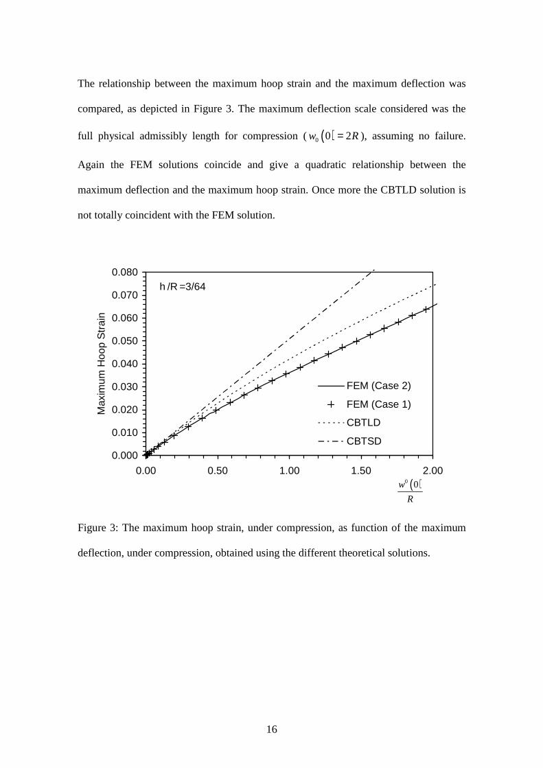
The relationship between the maximum hoop strain and the maximum deflection was

compared, as depicted in Figure 3. The maximum deflection scale considered was the

full physical admissibly length for compression (( )0 0 2w R= ), assuming no failure.

Again the FEM solutions coincide and give a quadratic relationship between the

maximum deflection and the maximum hoop strain. Once more the CBTLD solution is

not totally coincident with the FEM solution.

0.000

0.010

0.020

0.030

0.040

0.050

0.060

0.070

0.080

0.00 0.50 1.00 1.50 2.00

Max

imum

Hoo

p S

trai

n

FEM (Case 2)

FEM (Case 1)

CBTLD

CBTSD

( )0 0w

R

h /R =3/64

Figure 3: The maximum hoop strain, under compression, as function of the maximum

deflection, under compression, obtained using the different theoretical solutions.

17

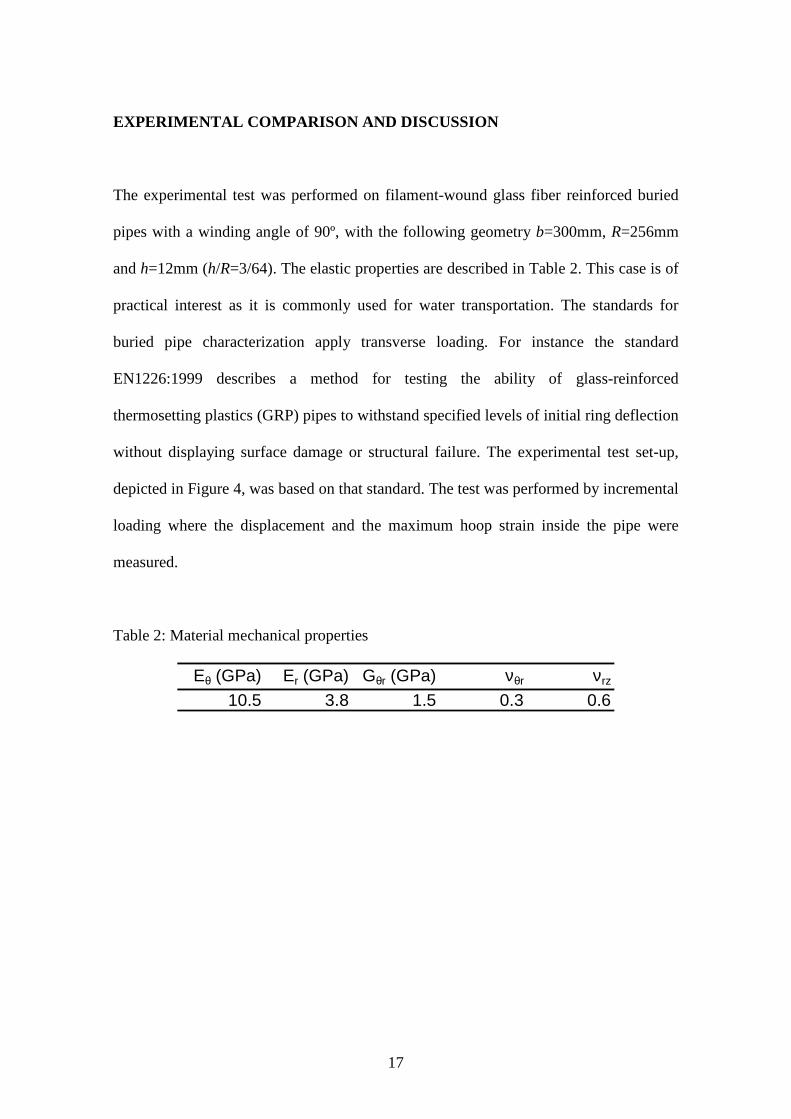
EXPERIMENTAL COMPARISON AND DISCUSSION

The experimental test was performed on filament-wound glass fiber reinforced buried

pipes with a winding angle of 90º, with the following geometry b=300mm, R=256mm

and h=12mm (h/R=3/64). The elastic properties are described in Table 2. This case is of

practical interest as it is commonly used for water transportation. The standards for

buried pipe characterization apply transverse loading. For instance the standard

EN1226:1999 describes a method for testing the ability of glass-reinforced

thermosetting plastics (GRP) pipes to withstand specified levels of initial ring deflection

without displaying surface damage or structural failure. The experimental test set-up,

depicted in Figure 4, was based on that standard. The test was performed by incremental

loading where the displacement and the maximum hoop strain inside the pipe were

measured.

Table 2: Material mechanical properties

Eθ (GPa) Er (GPa) Gθr (GPa) νθr νrz

10.5 3.8 1.5 0.3 0.6

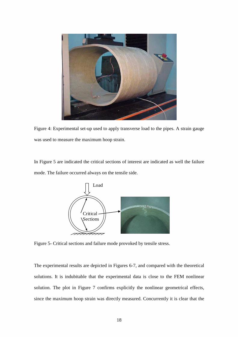
18

Figure 4: Experimental set-up used to apply transverse load to the pipes. A strain gauge

was used to measure the maximum hoop strain.

In Figure 5 are indicated the critical sections of interest are indicated as well the failure

mode. The failure occurred always on the tensile side.

Critical Sections

Load

Figure 5- Critical sections and failure mode provoked by tensile stress.

The experimental results are depicted in Figures 6-7, and compared with the theoretical

solutions. It is indubitable that the experimental data is close to the FEM nonlinear

solution. The plot in Figure 7 confirms explicitly the nonlinear geometrical effects,

since the maximum hoop strain was directly measured. Concurrently it is clear that the

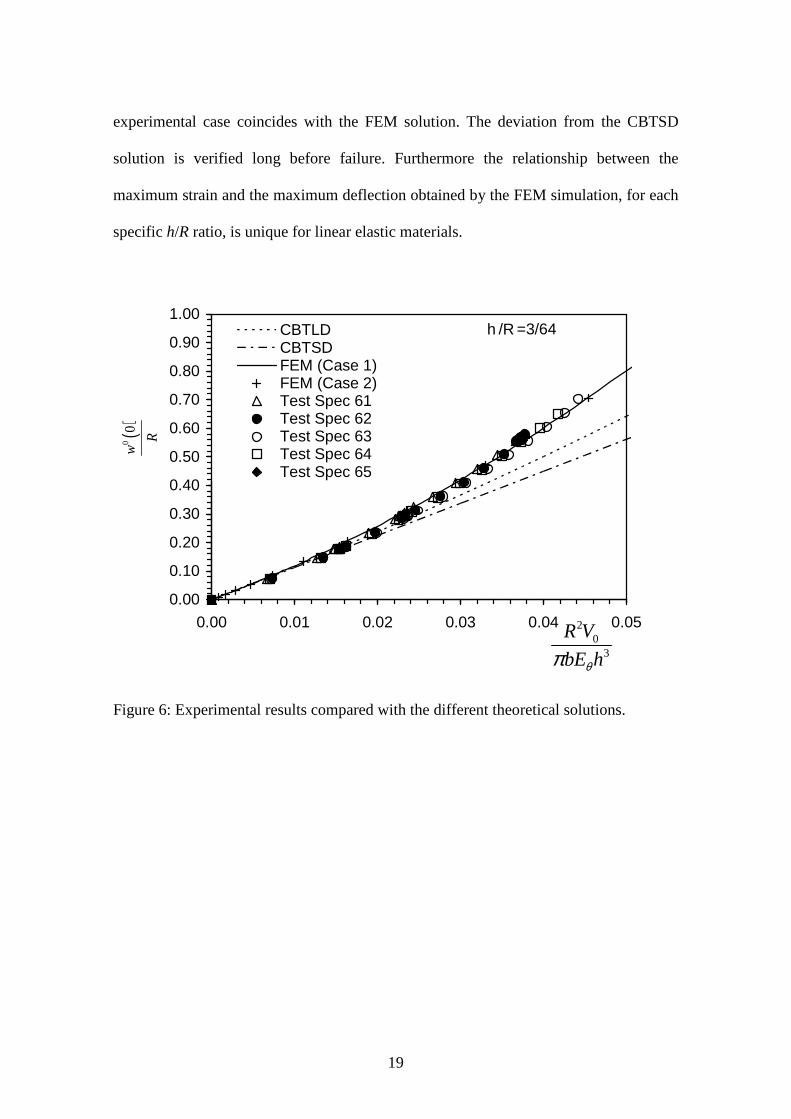
19

experimental case coincides with the FEM solution. The deviation from the CBTSD

solution is verified long before failure. Furthermore the relationship between the

maximum strain and the maximum deflection obtained by the FEM simulation, for each

specific h/R ratio, is unique for linear elastic materials.

0.00

0.10

0.20

0.30

0.40

0.50

0.60

0.70

0.80

0.90

1.00

0.00 0.01 0.02 0.03 0.04 0.05

CBTLDCBTSDFEM (Case 1)FEM (Case 2)Test Spec 61Test Spec 62Test Spec 63Test Spec 64Test Spec 65

20

3

R V

bE hθπ

()

00

w

R

h /R =3/64

Figure 6: Experimental results compared with the different theoretical solutions.

20

0.000

0.005

0.010

0.015

0.020

0.025

0.030

0.00 0.10 0.20 0.30 0.40 0.50 0.60

Max

imum

Hoo

p S

trai

nFEM (Case 2)FEM (Case 1)CBTLDCBTSDTest Spec 61Test Spec 62Test Spec 63Test Spec 64Test Spec 65

( )0 0w

R

h /R =3/64

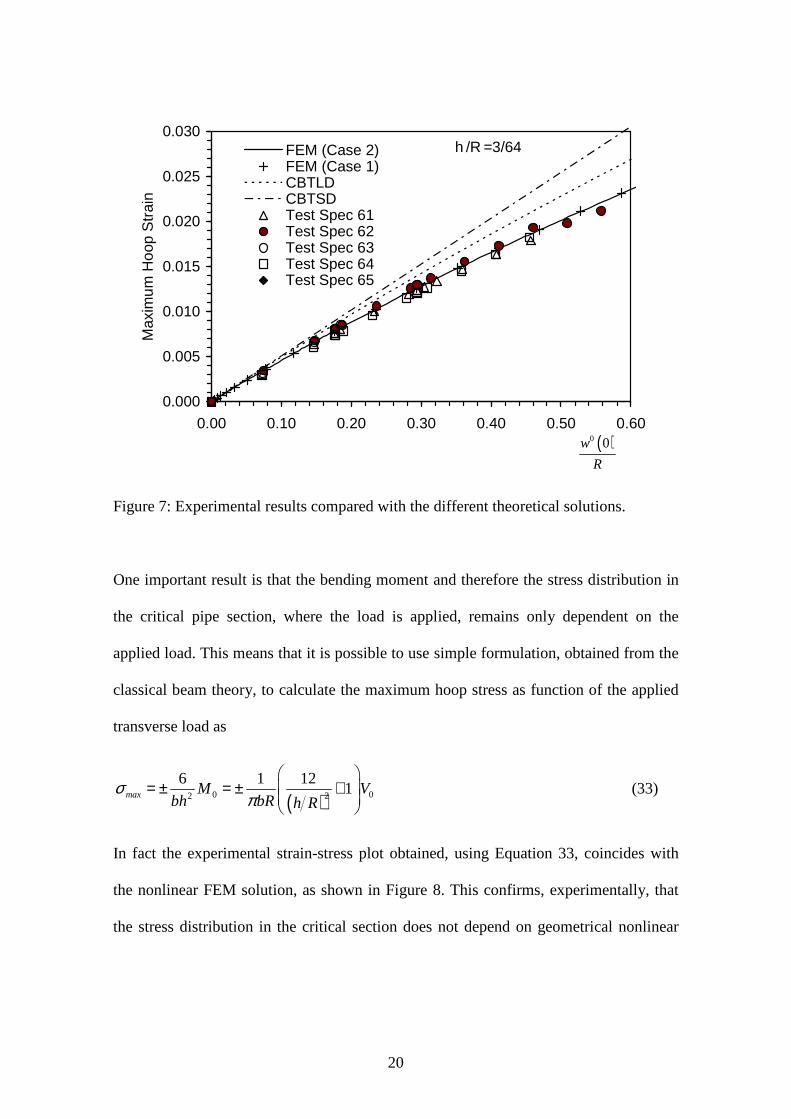
Figure 7: Experimental results compared with the different theoretical solutions.

One important result is that the bending moment and therefore the stress distribution in

the critical pipe section, where the load is applied, remains only dependent on the

applied load. This means that it is possible to use simple formulation, obtained from the

classical beam theory, to calculate the maximum hoop stress as function of the applied

transverse load as

( )0 022

6 1 121max M V

bh bR h Rσ

π

= ± = ± +

(33)

In fact the experimental strain-stress plot obtained, using Equation 33, coincides with

the nonlinear FEM solution, as shown in Figure 8. This confirms, experimentally, that

the stress distribution in the critical section does not depend on geometrical nonlinear

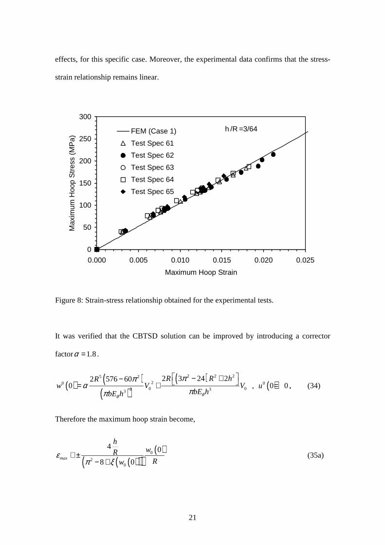
21

effects, for this specific case. Moreover, the experimental data confirms that the stress-

strain relationship remains linear.

0

50

100

150

200

250

300

0.000 0.005 0.010 0.015 0.020 0.025

Maximum Hoop Strain

Max

imum

Hoo

p S

tres

s (M

Pa)

FEM (Case 1)

Test Spec 61

Test Spec 62

Test Spec 63

Test Spec 64

Test Spec 65

h /R =3/64

Figure 8: Strain-stress relationship obtained for the experimental tests.

It was verified that the CBTSD solution can be improved by introducing a corrector

factor 1 8.α = .

( ) ( )( )

( )( )

2 2 25 220 0

0 02 33

2 3 24 22 576 600 0 0

R R hRw V V , u

bE hbE h θθ

ππα

ππ

− +− = + = , (34)

Therefore the maximum hoop strain become,

( )( )( )( )0

20

4 0

8 0max

hwR

Rwε

π ξ≅ ±

− + (35a)

22

where

( )( ) ( ) ( )22 20

01200 8 128

9

ww

Rξ π α π ≅ − + −

. (35b)

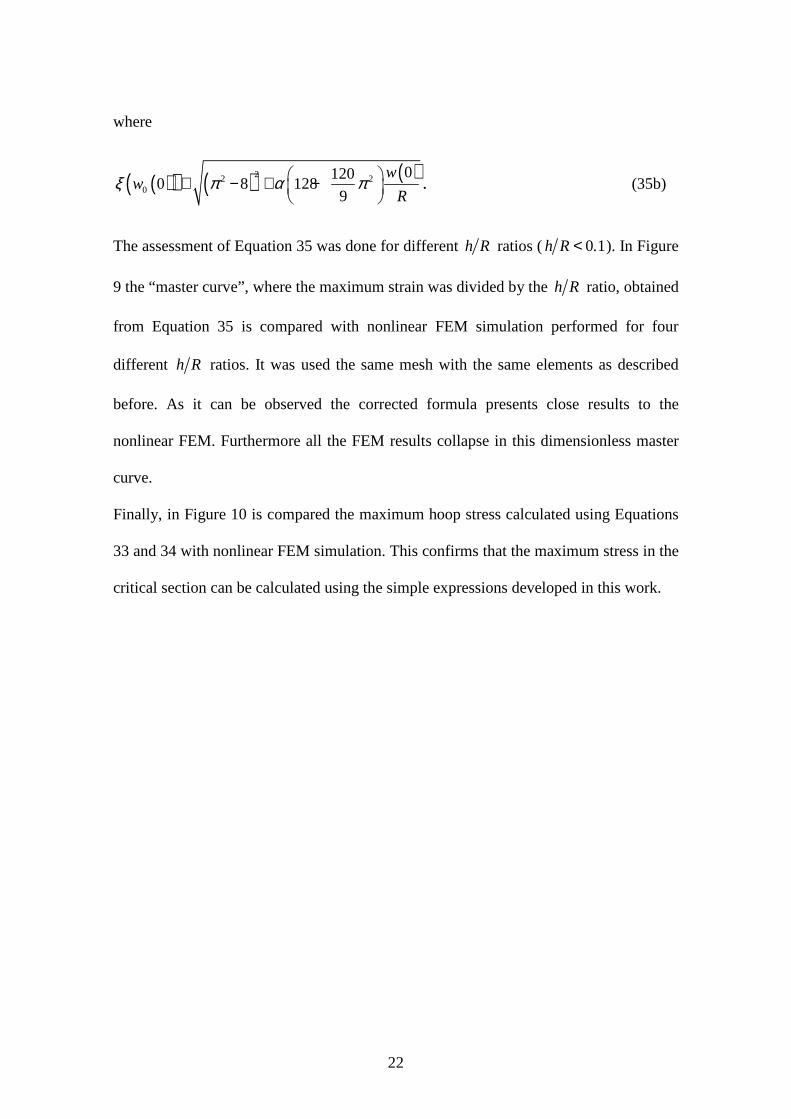
The assessment of Equation 35 was done for different h R ratios ( 0 1h R .< ). In Figure

9 the “master curve”, where the maximum strain was divided by the h R ratio, obtained

from Equation 35 is compared with nonlinear FEM simulation performed for four

different h R ratios. It was used the same mesh with the same elements as described

before. As it can be observed the corrected formula presents close results to the

nonlinear FEM. Furthermore all the FEM results collapse in this dimensionless master

curve.

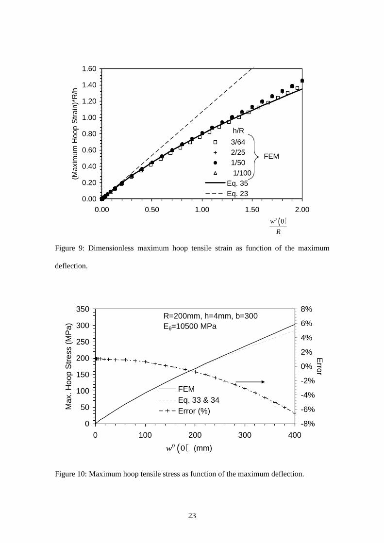
Finally, in Figure 10 is compared the maximum hoop stress calculated using Equations

33 and 34 with nonlinear FEM simulation. This confirms that the maximum stress in the

critical section can be calculated using the simple expressions developed in this work.

23

0.00

0.20

0.40

0.60

0.80

1.00

1.20

1.40

1.60

0.00 0.50 1.00 1.50 2.00

(Max

imum

Hoo

p S

trai

n)*R

/h

3/64 2/25 1/50 1/100Eq. 35Eq. 23

( )0 0w

R

h/R

FEM

Figure 9: Dimensionless maximum hoop tensile strain as function of the maximum

deflection.

0

50

100

150

200

250

300

350

0 100 200 300 400

(mm)

Max

. Hoo

p S

tres

s (M

Pa)

-8%

-6%

-4%

-2%

0%

2%

4%

6%

8%

Error

FEMEq. 33 & 34Error (%)

R=200mm, h=4mm, b=300Eθ=10500 MPa

( )0 0w

Figure 10: Maximum hoop tensile stress as function of the maximum deflection.

24

CONCLUSIONS

This work had the intention to show the importance of nonlinear effects in composite

structures. In this case glass-fiber reinforced (GRP) buried pipes were analysed. These

pipes were assumed as ring structures compressed by a transverse load. It was

experimentally verified that these structures sustain large deflections without damage or

failure. Therefore the classical formulation (CBTSD), based on the small displacements

theory, cannot be used. This includes many polymer matrix fiber-reinforced composite

structures which combine high strength with relative low stiffness. A formulation, based

on finite deformations theory was proposed and solved for the present case. In order to

have an analytical integral solution, it was used a simple approximation, i. e. the

influence of geometry of the deformed state on the bending moment distribution was

not included. Although the solution (CBTLD) was not completely correct, it permitted

obtaining analytical integral expressions. From this solution it was possible to perform a

dimensionless parametric analysis. Moreover, dimensionless relationship between the

load, the maximum deflection and the maximum hoop strain was obtained.

A 2D FEM simulation using a large displacement formulation, with a very refined

mesh, was performed. Two different cases were simulated to verify the dimensionless

relationships obtained using the CBTLD. Although the CBTLD results didn’t match

exactly the FEM solution, the general solution trend of dimensionless relationships was

similar. A simple correction of CBTLD was proposed and assessed. This allowed

obtaining a simple law between maximum deflection and maximum strain at the critical

section.

25

Finally the theoretical results were compared with experimental data. It was tested a

structure of practical interest used for water transportation; filament-wound glass-fiber

reinforced buried pipes with a winding angle of 90º. The experimental results confirm

the FEM solution and validate the general trends of the CBTLD approach. These results

confirm experimentally that for some composite structures the geometrical nonlinear

effects start very early, long before damage or failure take place. Therefore direct strain

measurement becomes important, since the information from the maximum deflection is

not enough to evaluate completely the structural performance. Since ring stiffness

decrease with deflection, it is important not mistake nonlinear geometrical effects for

damage.

ACKNOWLEDGEMENTS

The research hereby presented was supported by Fundação para a Ciência e Tecnologia

(Ministério da Ciência e do Ensino Superior) through the Project

POCTI/EME/47734/2002. The valuable contributions of graduated students Hugo Faria

and Alcides Sá are also gratefully acknowledge.

REFERENCES

1. Bishopp K E and Drucker D C, 1945. Large deflections of cantilever beams Quarterly of Applied Mathematics 3 (3): 272-275.

2. Tse PC, Lai TC, So CK, 1997. A note on large deflection of elastic composite circular springs under tension and in push-pull configuration. Composite Structures 40 (3-4): 223-230.

26

3. Tse PC, Lung CT, 2000. Large deflections of elastic composite circular springs under uniaxial tension. International Journal of Non-linear Mechanics 35: 293-307.

4. Tse, P. C., Lai, T. C., So, C. K. and Cheng, C. M., 1994. Large deflection of elastic composite circular springs under uniaxial compression. International Journal of Non-linear Mechanics 29:781-798.

5. Sheinman I., 1982. Large Deflection of Curved Beam with Shear Deformation. Journal of the Engineering Mechanics Division-ASCE 108 (4): 636-647.

6. Belendez T, Neipp C, Belendez A., 2002. Large and small deflections of a cantilever beam. European Journal of Physics 23 (3): 371-379.

7. Carrillo ES., 2006. The cantilevered beam: an analytical solution for general deflections of linear-elastic materials. European Journal of Physics; 27 (6): 1437.

8. González C., LLorca J., 2005. Stiffness of a curved beam subjected to axial load and large displacements. International Journal of Solids and Structures 42(5-6):1537-1545.

9. Lim CW, Wang CM, Kitipornchai S., 1997. Timoshenko Curved Beam Bending Solutions in Terms of Euler-Bernoulli Solutions. Archive of Applied Mechanics 67:179-190.

10. Ragab A, Bayoumi S., 1999. Engineering Solid Mechanics: Fundamentals and applications. CRC Press.

11. Qatu, M. S., 1993. Theories and analysis in thin and moderately thick laminated composite curved beams. Int. J. Solids Struct. 20: 2743–2756.

12. Kreyszig Erwin, 2000. Advanced Engineering Mathematics. John Wiley & Sons, New York.

13. Williams J.G, 1980. Stress Analysis of Polymers, 2nd Edition. Ellis Hordwood series in Engineering Science.

14. Ambartsumyan SA, 1970. Theory of Anisotropic Plates. Progress in Materials Science Series, Volume 11. Editor Ashton JE. Technomic publication, USA.

27

APPENDIX A

The system of differential equations to be solved for the radial and tangential

displacements is

( ) ( )( )

( )( )

220 3

0 00 032 2 3 2 2

20 30

0 033 2 2

12 1121 1 144

212 12

12 11 144

12

R cosM Ru Rw M V

R bE hbE h R h bE h R h

R cosw Ru M V

R bE hbE h R h

θθ θ

θθ

θθθ

θθθ

− ∂ + = − + ∂ − − − ∂− + = + ∂ − (A1)

The boundary conditions are given by

( ) ( )( )

( ) ( )

0 0

0

0 00 0

0 0

0

0 0

u u

w

w wu u

π

π

πθ θ

= =

=

∂ ∂− + = − + = ∂ ∂

(A2)

The moment 0M is readily obtained using the boundary conditions,

2

0 0

2

6

R hM V

Rπ π

= − −

. (A3)

The solution of the system of differential equations is obtained using the standard

mathematical procedures (Erwin Kreyszig, Advanced Engineering Mathematics, New

York: John Wiley & Sons, 2000).

( )( )

( )

( )( )

50 2 2

23

22 2 2 20

3 2

302 3

236 108 36

288 12 36 6 2 144 54 144 288

6 24 2 3 3 12 12

Rw sin

b E h

cos cos V

sin cos cosR R V

b E h b E h

θ

θ θ

θ π π θ θπ

π θπ θ π θ θ π πθ

π θ π π θπ π θ θπ π

= − − +

− − + − − + +

− + − − + +

, (A4)

28

( )( )

( )

( )( )

50 2

23

22 2 3 20

2 2 3 2

302 3

248 288 36

36 36 144 144 12 2 288

12 6 12 3 3 122 2

Ru sin

b E h

cos sin V

cos sin sinR R V

b E h b E h

θ

θ θ

θ π θπ θπ

θπ θ π π θ π π θ θ

π θ π πθ π θπ π θ θπ π

= − − +

− − + − −

− + − − − −

, (A4)