Embed Size (px)
Citation preview
North America –Akselos, Inc. ֎ Switzerland –Akselos S.A.
Component-Based Model Reduction for
Industrial Scale Problems
Dr. David Knezevic, CTO
1 1. Context
2. SCRBE
3. Coupled SCRBE/FE for Nonlinear
Context
In many industries, engineers need to model large,
complex systems:
• Ships
• Oil platforms
• Mining machinery
• Wind turbines
• Aircraft
• …
Detailed modeling of large systems with FE is
considered impractical in most circumstances
Context
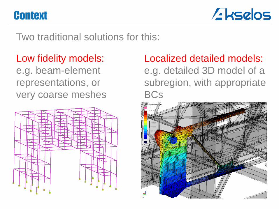
Two traditional solutions for this:
Low fidelity models:
e.g. beam-element
representations, or
very coarse meshes
Localized detailed models:
e.g. detailed 3D model of a
subregion, with appropriate
BCs
Context
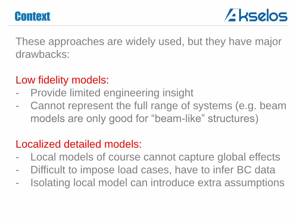
These approaches are widely used, but they have major
drawbacks:
Low fidelity models:
- Provide limited engineering insight
- Cannot represent the full range of systems (e.g. beam
models are only good for “beam-like” structures)
Localized detailed models:
- Local models of course cannot capture global effects
- Difficult to impose load cases, have to infer BC data
- Isolating local model can introduce extra assumptions
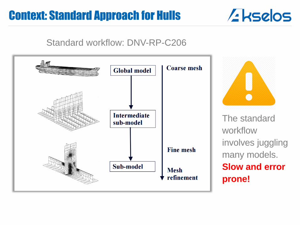
Context: Standard Approach for Hulls
Standard workflow: DNV-RP-C206
The standard
workflow
involves juggling
many models.
Slow and error
prone!
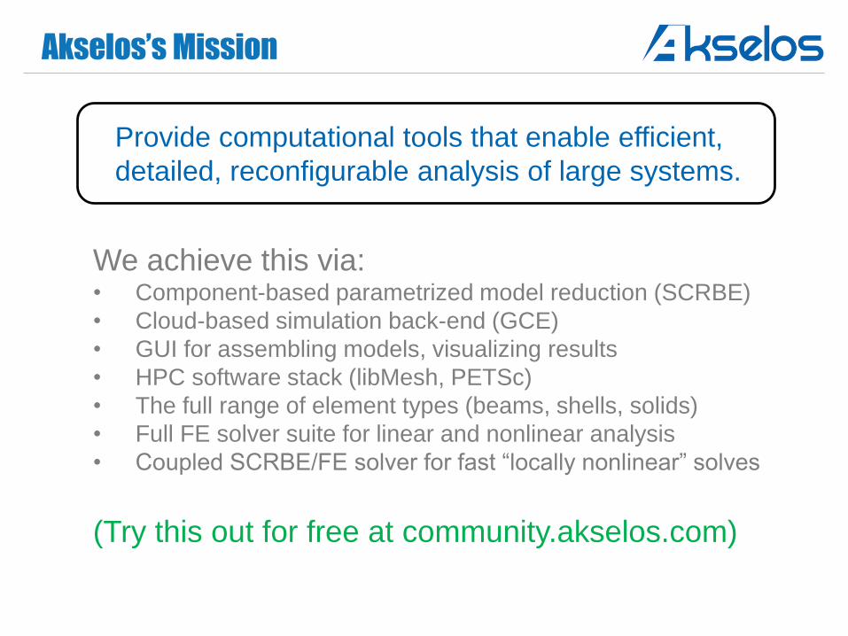
Akselos’s Mission
We achieve this via:• Component-based parametrized model reduction (SCRBE)
• Cloud-based simulation back-end (GCE)
• GUI for assembling models, visualizing results
• HPC software stack (libMesh, PETSc)
• The full range of element types (beams, shells, solids)
• Full FE solver suite for linear and nonlinear analysis
• Coupled SCRBE/FE solver for fast “locally nonlinear” solves
(Try this out for free at community.akselos.com)
Provide computational tools that enable efficient,
detailed, reconfigurable analysis of large systems.
2 1. Context
2. SCRBE
3. Coupled SCRBE/FE for Nonlinear
SCRBE: Static Condensation + RB
SCRBE: Static Condensation Reduced Basis Element(Huynh, Knezevic, Patera, “A Static Condensation Reduced Basis Element
Method: Approximation and A Posteriori Error Estimation", M2AN, 2012.)
Several related approaches in the literature:• Maday, Ronquist: RB Element Method, Lagrange multipliers to “glue” non-
conforming approximations
• Chen, Hesthaven, Maday: Seamless Reduced Basis Element Method, DG
formulation to avoid Lagrange multipliers
• Nguyen: Multiscale Reduced Basis method, similar to MsFEM but uses RB for
cell problems
• Iapichino, Quarteroni, Rozza: Reduced Basis Hybrid method, couples
components via coarse grid and Lagrange multipliers
• Heinkenschloss et al.: Balanced truncation model reduction on subdomains
coupled to FE
• Craig-Bampton, Component Mode Synthesis: Widely used in industry for non-
parametrized eigenvalue or dynamic problems
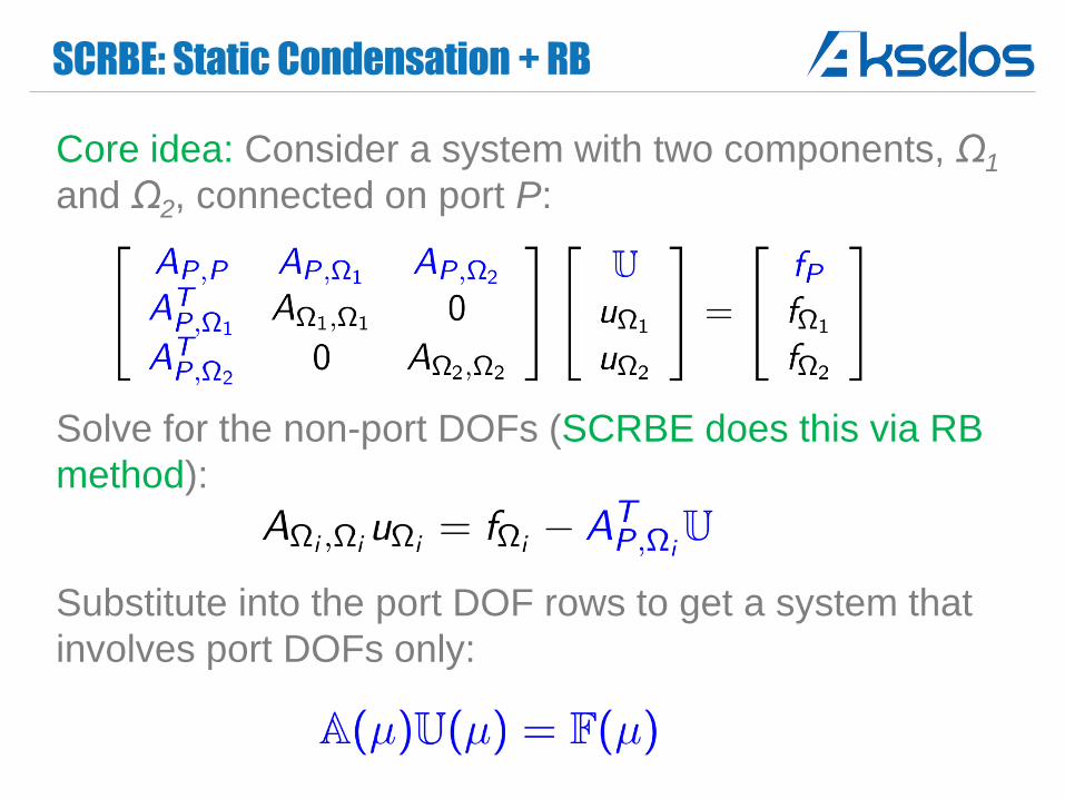
SCRBE: Static Condensation + RB
Core idea: Consider a system with two components, Ω1
and Ω2, connected on port P:
Solve for the non-port DOFs (SCRBE does this via RB
method):
Substitute into the port DOF rows to get a system that
involves port DOFs only:
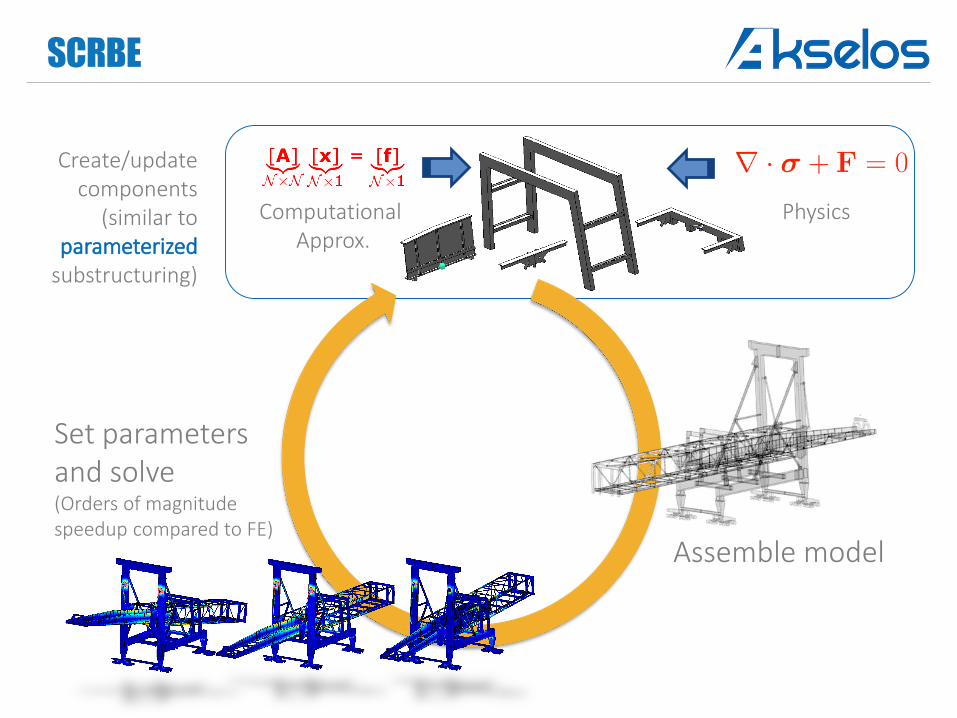
SCRBE
Set parameters and solve (Orders of magnitude speedup compared to FE)
Assemble model
Create/update components
(similar to parameterized
substructuring)
PhysicsComputational Approx.
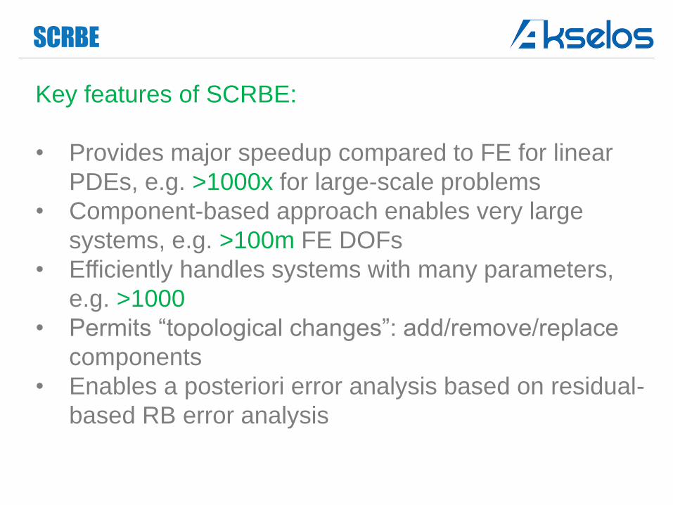
SCRBE
Key features of SCRBE:
• Provides major speedup compared to FE for linear
PDEs, e.g. >1000x for large-scale problems
• Component-based approach enables very large
systems, e.g. >100m FE DOFs
• Efficiently handles systems with many parameters,
e.g. >1000
• Permits “topological changes”: add/remove/replace
components
• Enables a posteriori error analysis based on residual-
based RB error analysis
SCRBE: Port Modes
Classical substructuring typically uses “all” DOFs on a
port
Craig-Bampton, CMS (typically used for modal/dynamic)
uses truncated port representations
We advocate truncated port representations in SCRBE:
• Retains good accuracy in practice (typically <1%
error wrt FE, sufficient for engineering purposes)
• Provides larger speedup, reduces data footprint
Several port truncation methods for SCRBE have been
published: pairwise methods, empirical, “optimal modes”
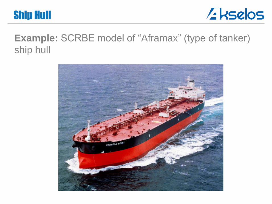
Ship Hull
Example: SCRBE model of “Aframax” (type of tanker)
ship hull
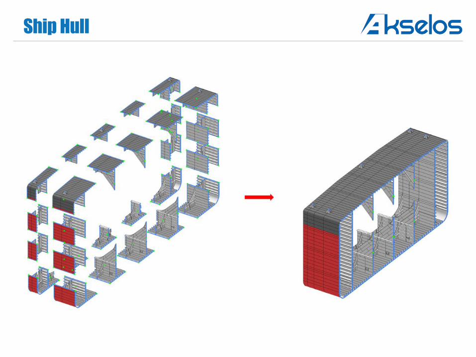
Ship Hull
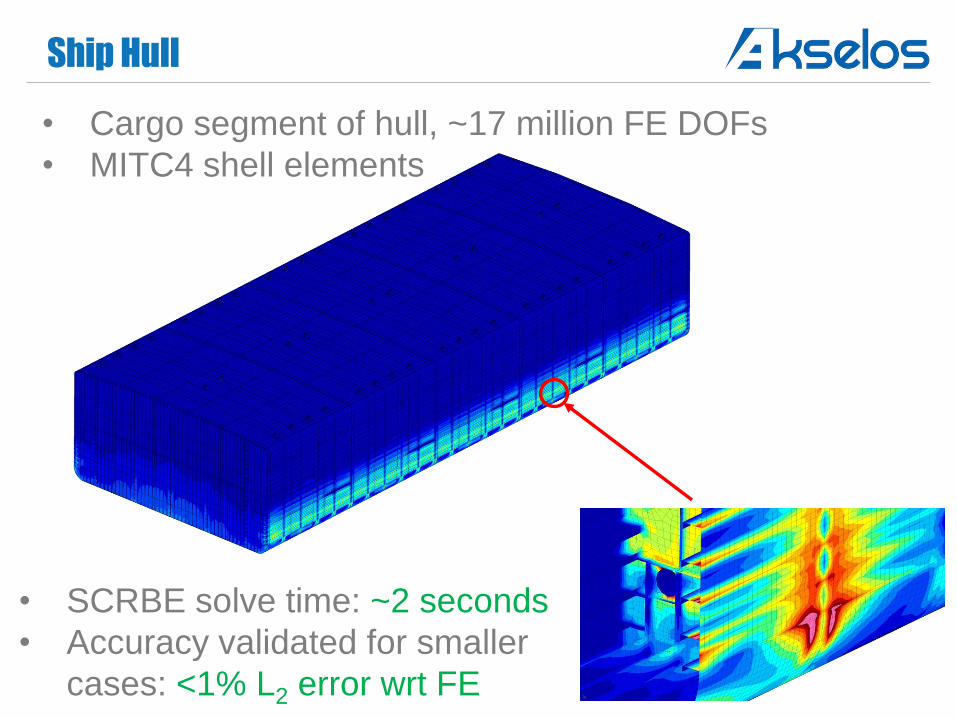
Ship Hull
• Cargo segment of hull, ~17 million FE DOFs
• MITC4 shell elements
• SCRBE solve time: ~2 seconds
• Accuracy validated for smaller
cases: <1% L2 error wrt FE
Ship Hull
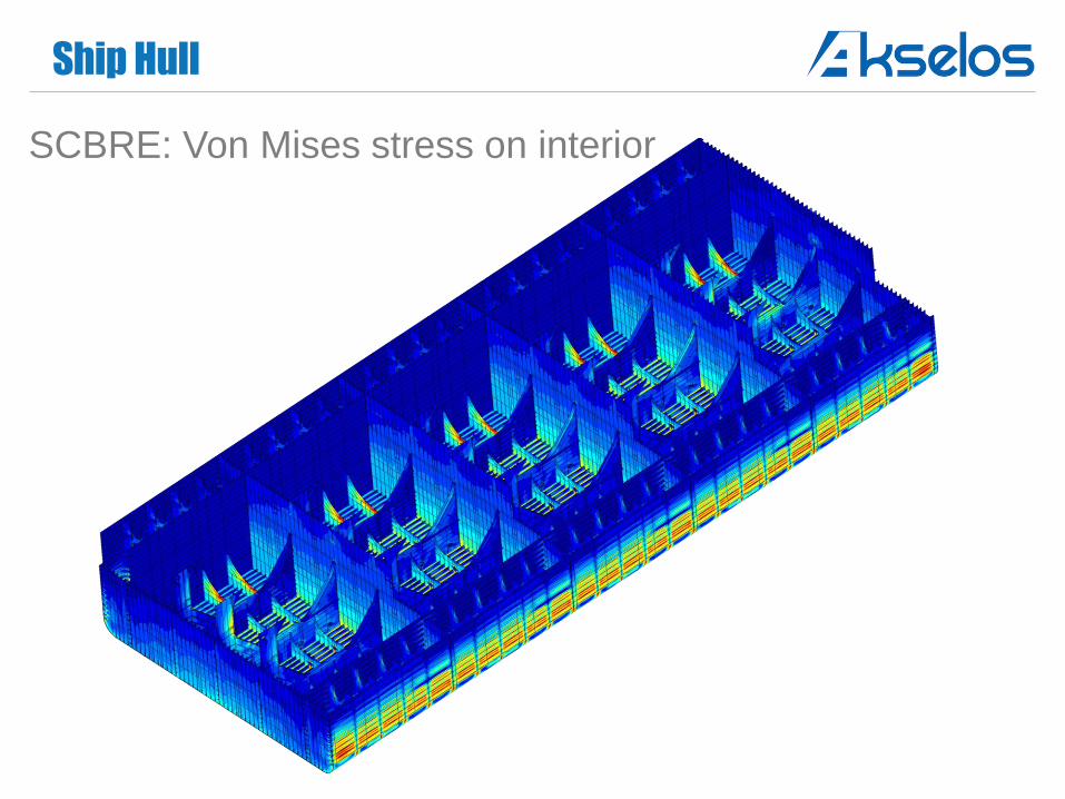
SCBRE: Von Mises stress on interior
Ship Hull
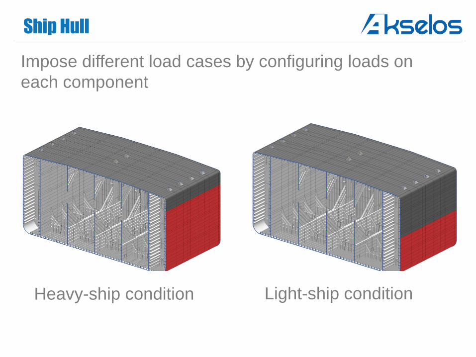
Impose different load cases by configuring loads on
each component
Heavy-ship condition Light-ship condition
Ship Hull
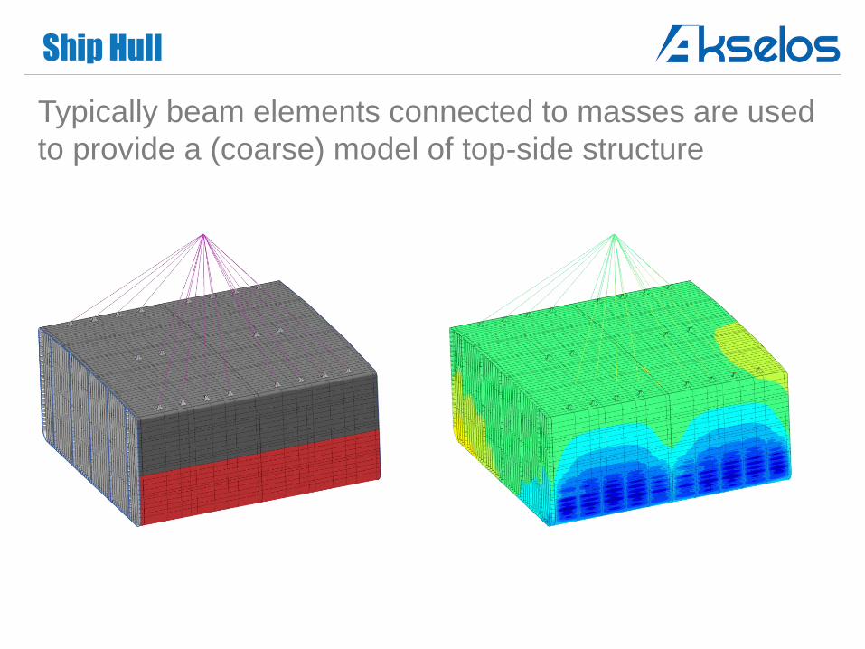
Typically beam elements connected to masses are used
to provide a (coarse) model of top-side structure
Ship Hull
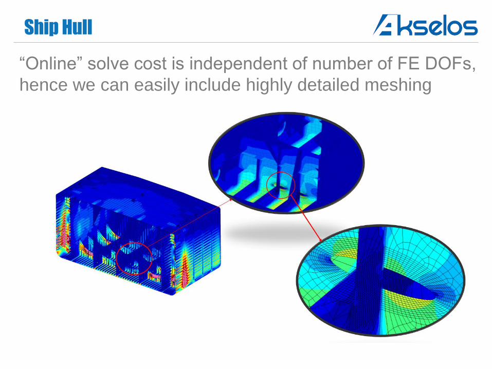
“Online” solve cost is independent of number of FE DOFs,
hence we can easily include highly detailed meshing
Ship Hull
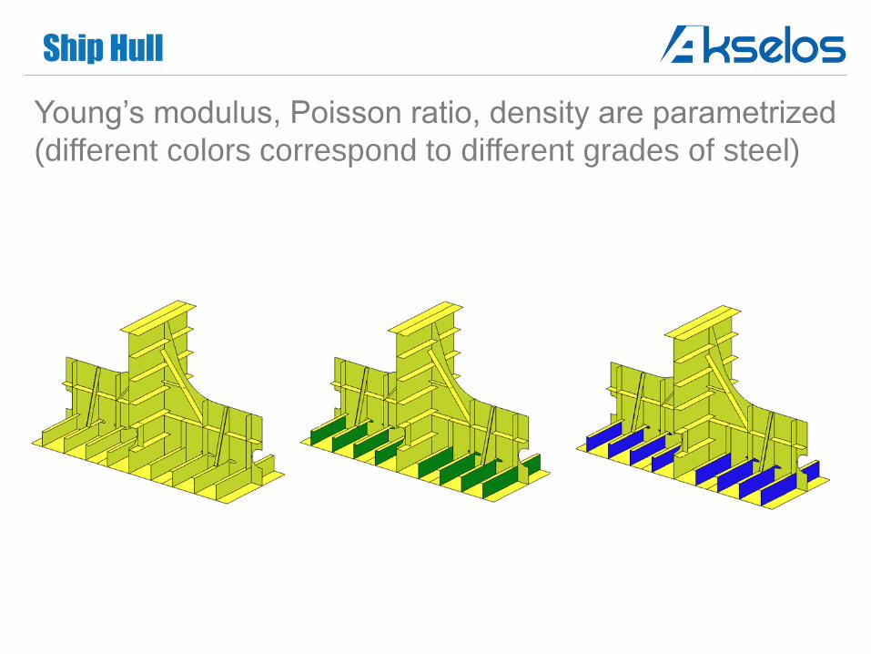
Young’s modulus, Poisson ratio, density are parametrized
(different colors correspond to different grades of steel)
Ship Hull
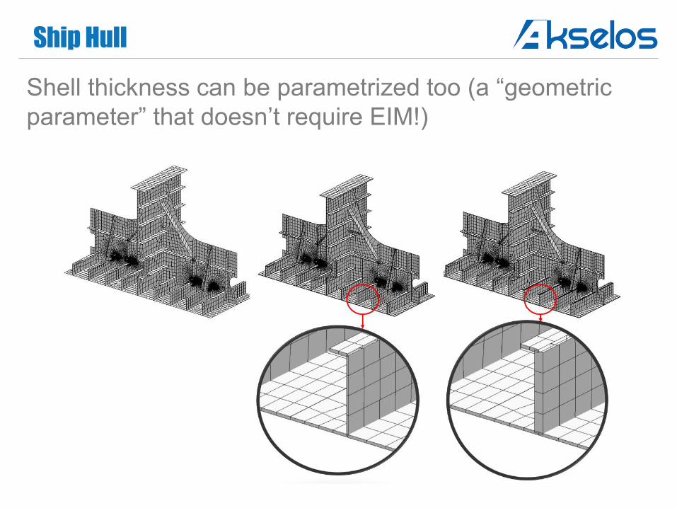
Shell thickness can be parametrized too (a “geometric
parameter” that doesn’t require EIM!)
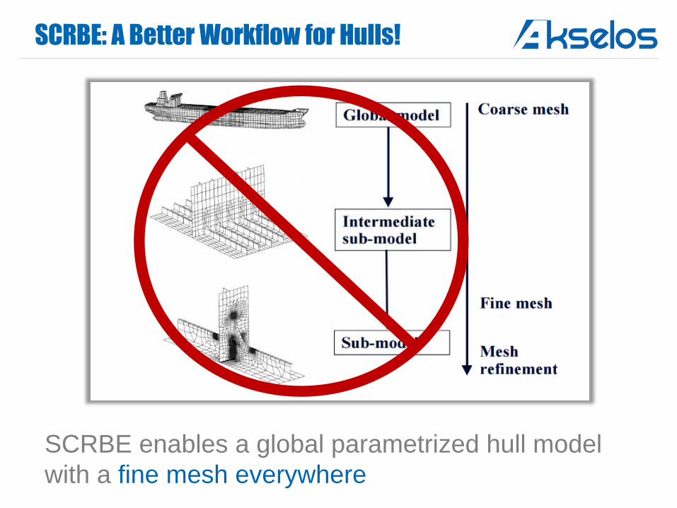
SCRBE: A Better Workflow for Hulls!
SCRBE enables a global parametrized hull model
with a fine mesh everywhere
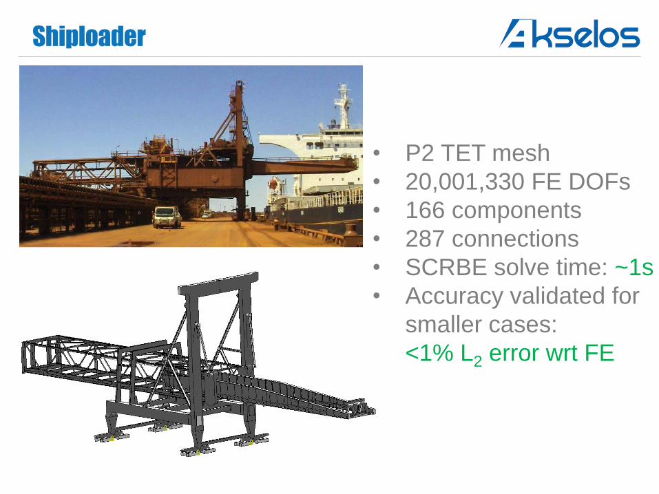
Shiploader
• P2 TET mesh
• 20,001,330 FE DOFs
• 166 components
• 287 connections
• SCRBE solve time: ~1s
• Accuracy validated for
smaller cases:
<1% L2 error wrt FE
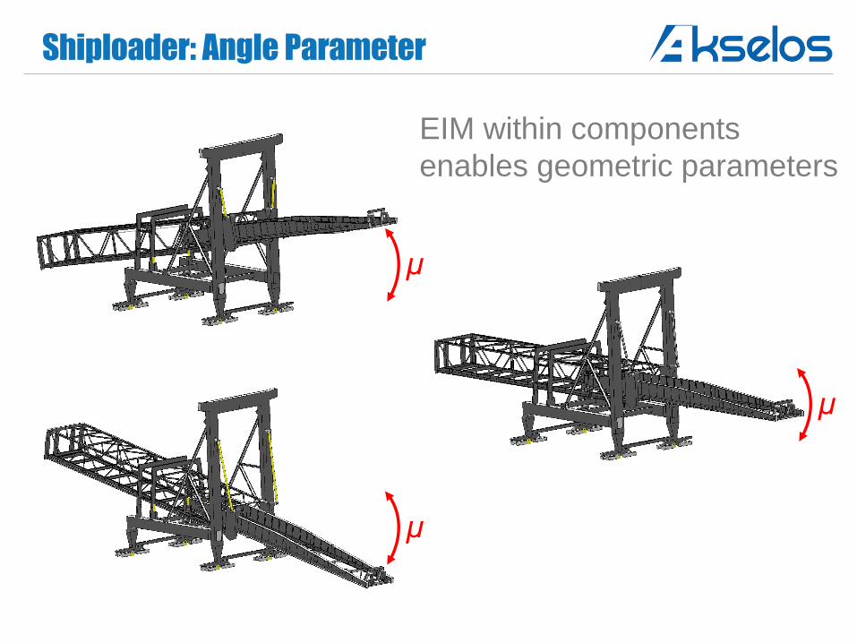
Shiploader: Angle Parameter
EIM within components
enables geometric parameters
μ
μ
μ
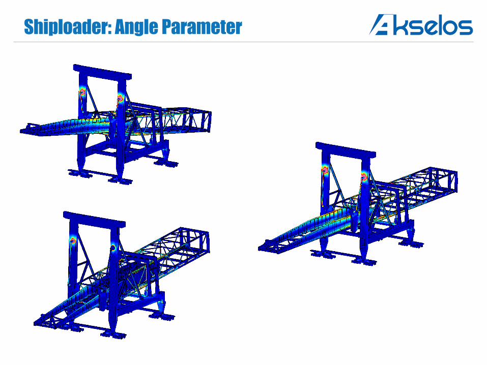
Shiploader: Angle Parameter
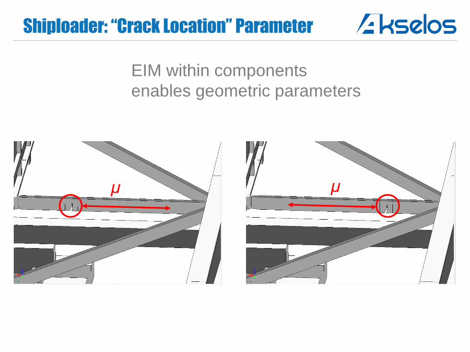
Shiploader: “Crack Location” Parameter
EIM within components
enables geometric parameters
μ μ
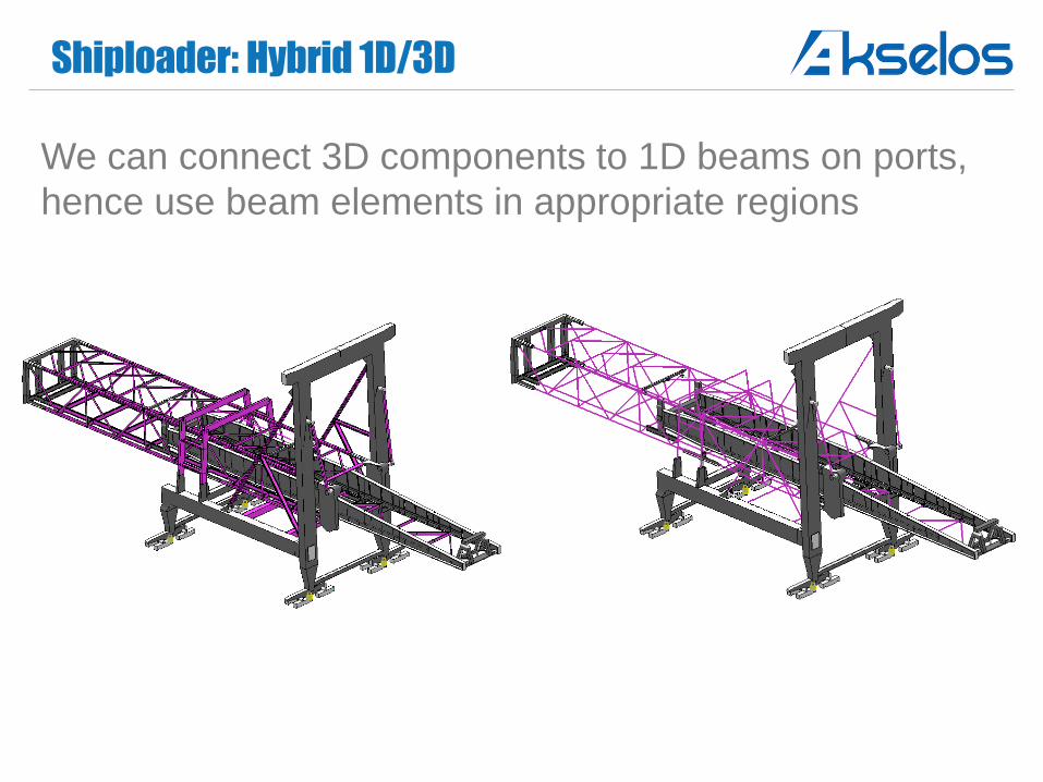
Shiploader: Hybrid 1D/3D
We can connect 3D components to 1D beams on ports,
hence use beam elements in appropriate regions
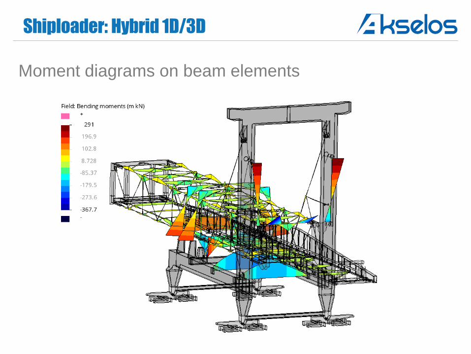
Shiploader: Hybrid 1D/3D
Moment diagrams on beam elements
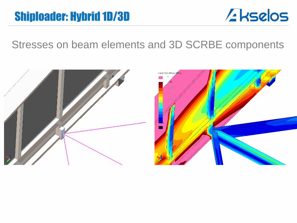
Shiploader: Hybrid 1D/3D
Stresses on beam elements and 3D SCRBE components
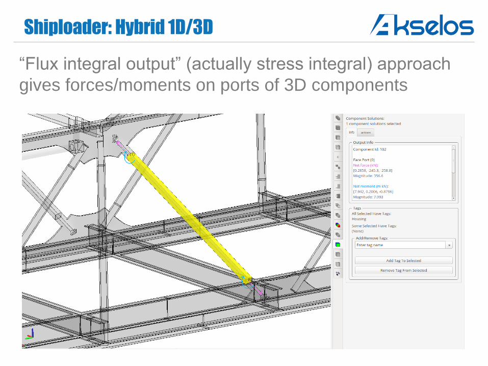
Shiploader: Hybrid 1D/3D
“Flux integral output” (actually stress integral) approach
gives forces/moments on ports of 3D components
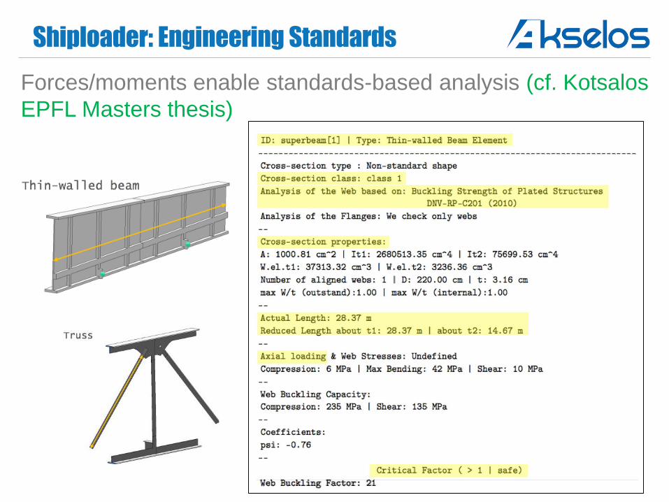
Shiploader: Engineering Standards
Forces/moments enable standards-based analysis (cf. Kotsalos
EPFL Masters thesis)
Shiploader: FE Buckling
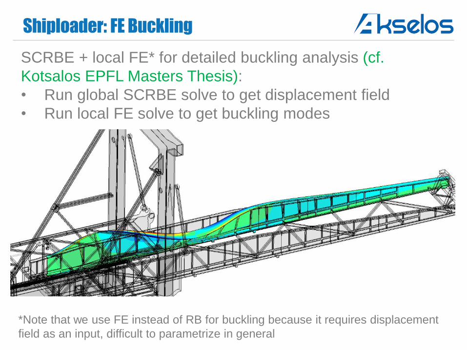
SCRBE + local FE* for detailed buckling analysis (cf.
Kotsalos EPFL Masters Thesis):
• Run global SCRBE solve to get displacement field
• Run local FE solve to get buckling modes
*Note that we use FE instead of RB for buckling because it requires displacement
field as an input, difficult to parametrize in general
Wind Turbine: SCRBE Eigenmodes
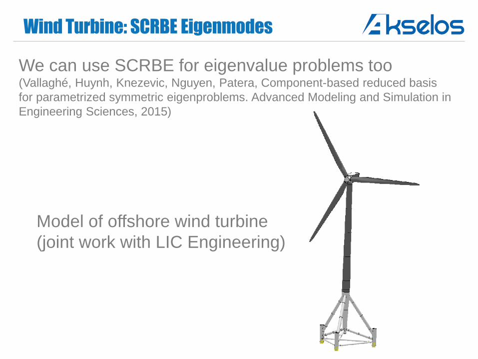
We can use SCRBE for eigenvalue problems too(Vallaghé, Huynh, Knezevic, Nguyen, Patera, Component-based reduced basis
for parametrized symmetric eigenproblems. Advanced Modeling and Simulation in
Engineering Sciences, 2015)
Model of offshore wind turbine
(joint work with LIC Engineering)
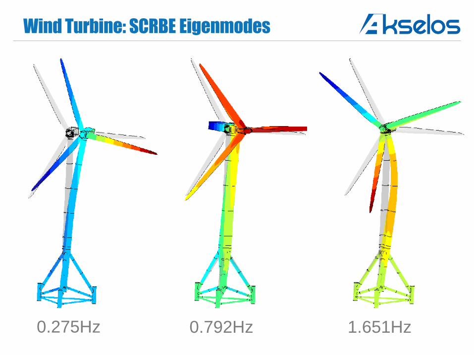
Wind Turbine: SCRBE Eigenmodes
0.275Hz 0.792Hz 1.651Hz
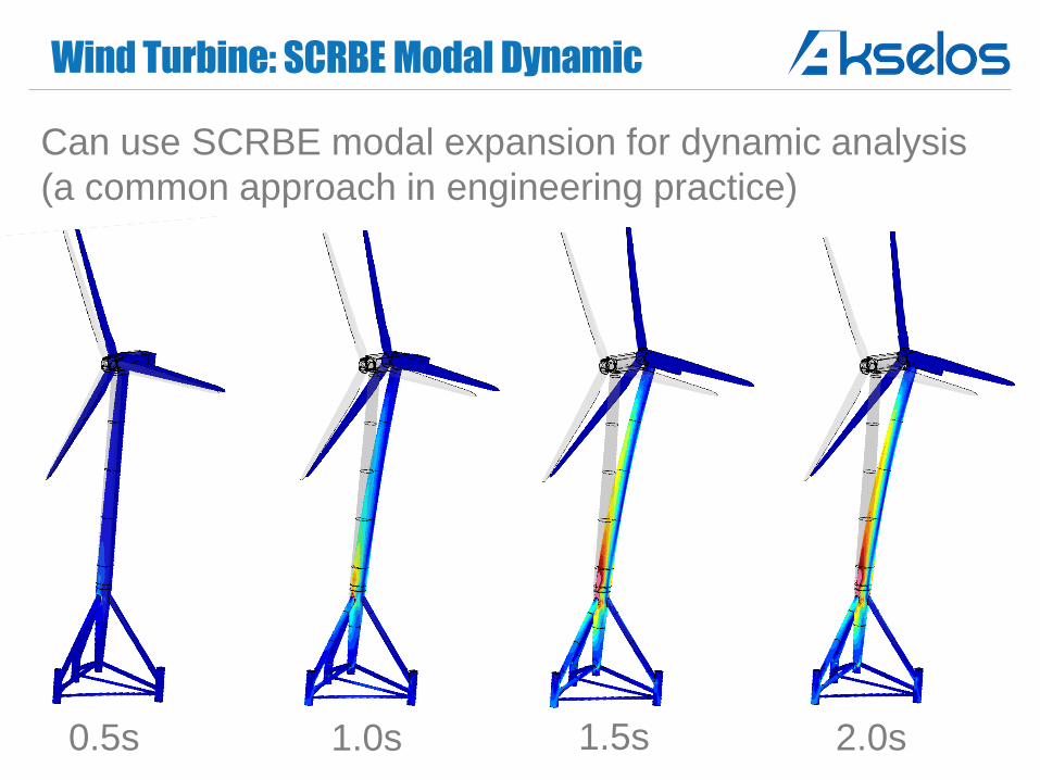
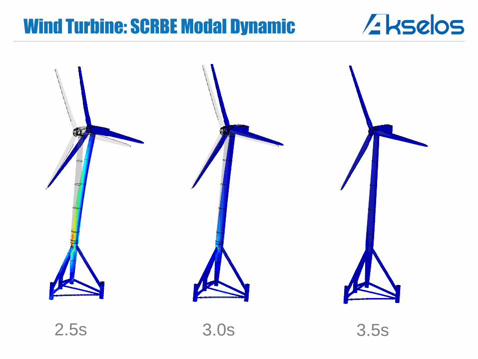
Wind Turbine: SCRBE Modal Dynamic
Can use SCRBE modal expansion for dynamic analysis
(a common approach in engineering practice)
0.5s 1.0s 1.5s 2.0s
Wind Turbine: SCRBE Modal Dynamic
2.5s 3.0s 3.5s
3 1. Context
2. SCRBE
3. Coupled SCRBE/FE for Nonlinear
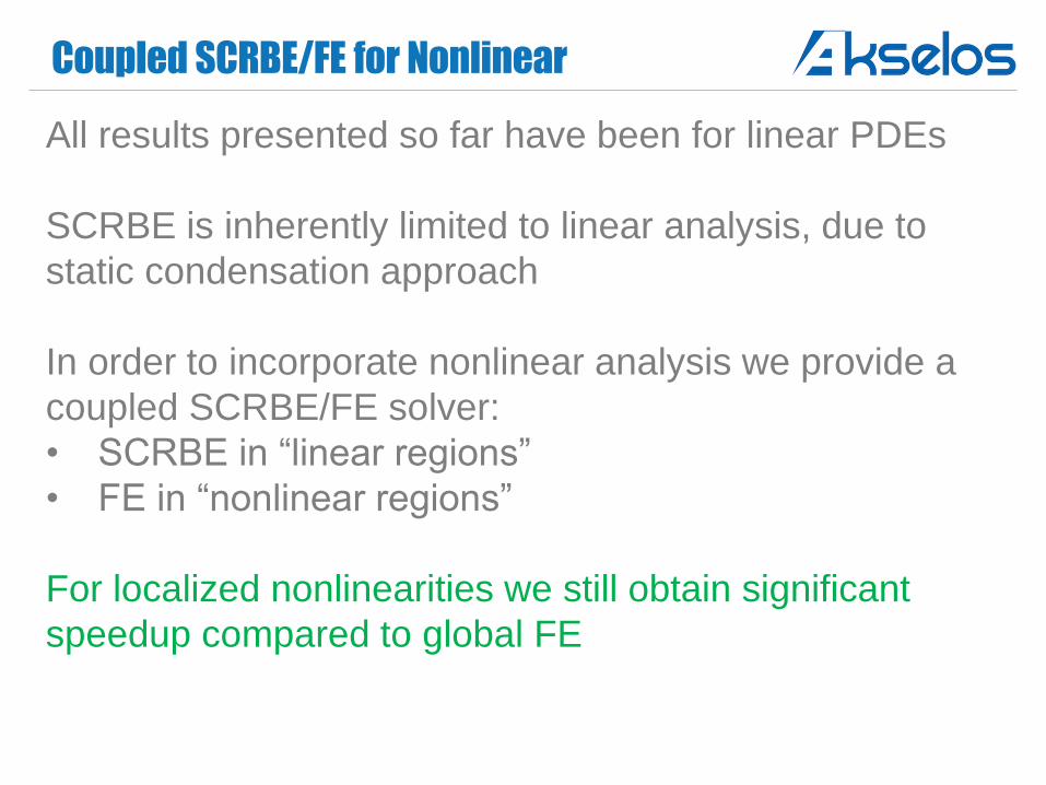
Coupled SCRBE/FE for Nonlinear
All results presented so far have been for linear PDEs
SCRBE is inherently limited to linear analysis, due to
static condensation approach
In order to incorporate nonlinear analysis we provide a
coupled SCRBE/FE solver:
• SCRBE in “linear regions”
• FE in “nonlinear regions”
For localized nonlinearities we still obtain significant
speedup compared to global FE
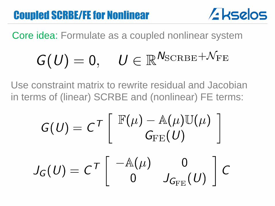
Coupled SCRBE/FE for Nonlinear
Core idea: Formulate as a coupled nonlinear system
Use constraint matrix to rewrite residual and Jacobian
in terms of (linear) SCRBE and (nonlinear) FE terms:
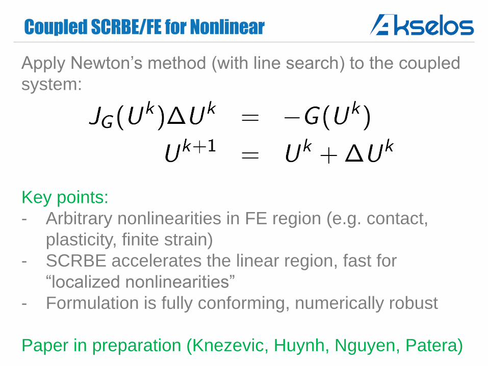
Coupled SCRBE/FE for Nonlinear
Apply Newton’s method (with line search) to the coupled
system:
Key points:
- Arbitrary nonlinearities in FE region (e.g. contact,
plasticity, finite strain)
- SCRBE accelerates the linear region, fast for
“localized nonlinearities”
- Formulation is fully conforming, numerically robust
Paper in preparation (Knezevic, Huynh, Nguyen, Patera)
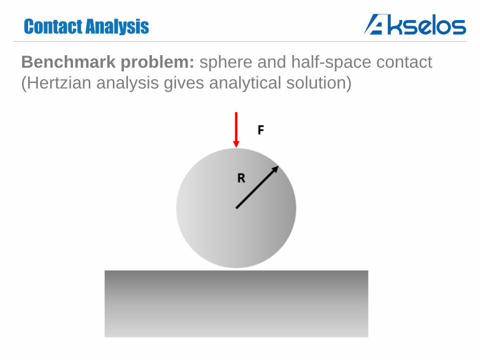
Contact Analysis
Benchmark problem: sphere and half-space contact
(Hertzian analysis gives analytical solution)
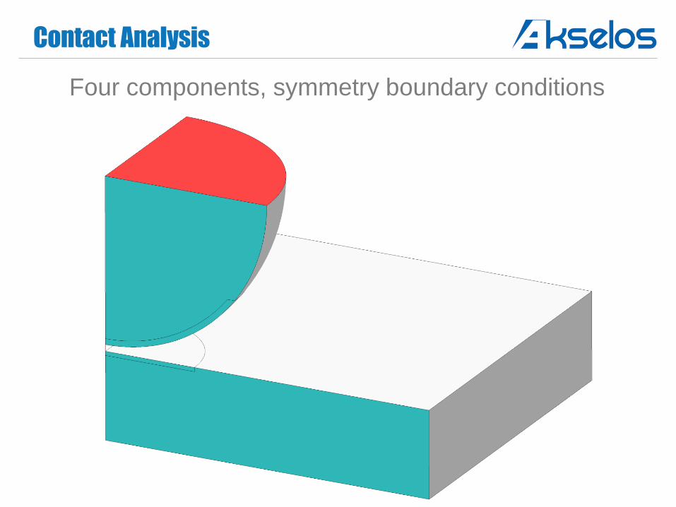
Contact Analysis
Four components, symmetry boundary conditions
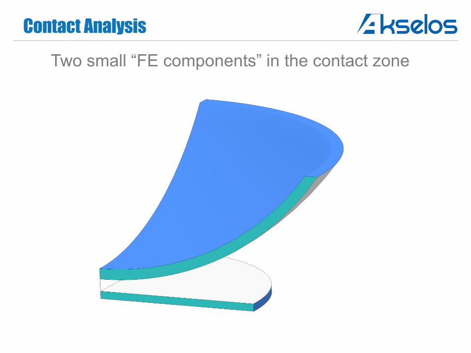
Contact Analysis
Two small “FE components” in the contact zone
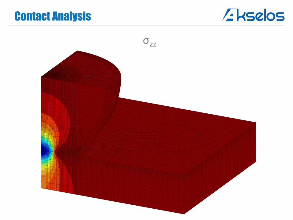
Contact Analysis
σzz
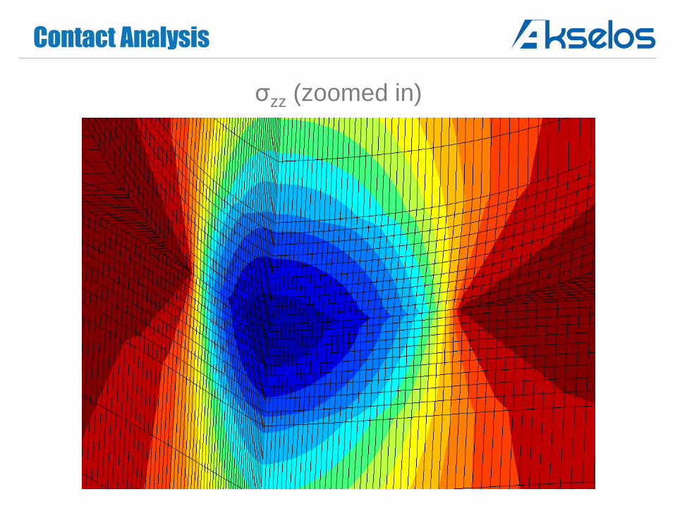
Contact Analysis
σzz (zoomed in)
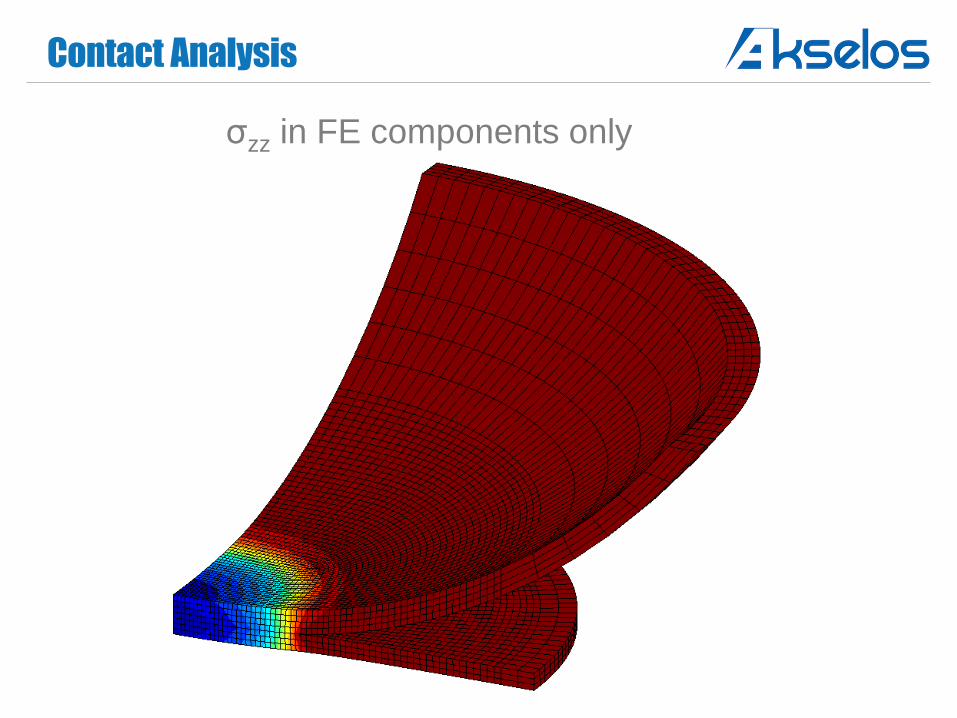
Contact Analysis
σzz in FE components only
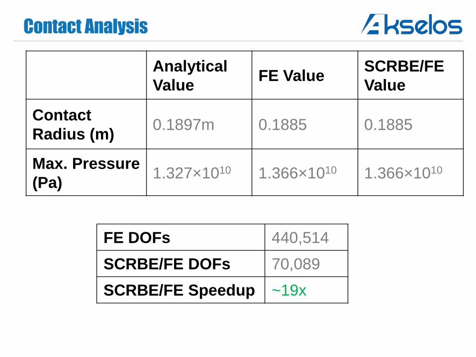
Contact Analysis
Analytical
ValueFE Value
SCRBE/FE
Value
Contact
Radius (m)0.1897m 0.1885 0.1885
Max. Pressure
(Pa)1.327×10¹⁰ 1.366×10¹⁰ 1.366×10¹⁰
FE DOFs 440,514
SCRBE/FE DOFs 70,089
SCRBE/FE Speedup ~19x
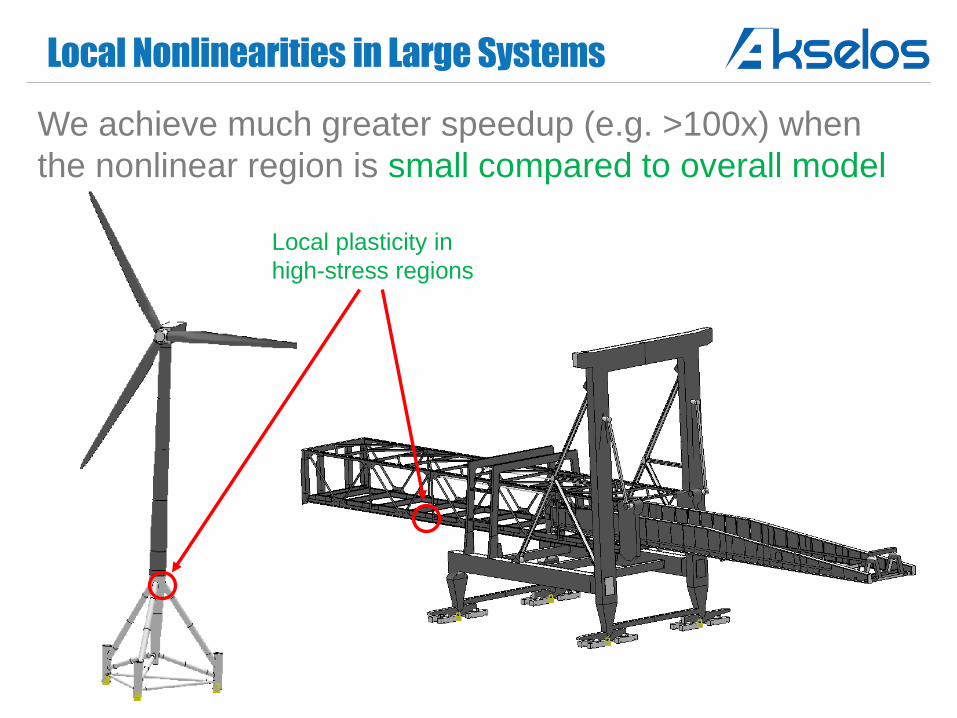
Local Nonlinearities in Large Systems
We achieve much greater speedup (e.g. >100x) when
the nonlinear region is small compared to overall model
Local plasticity in
high-stress regions
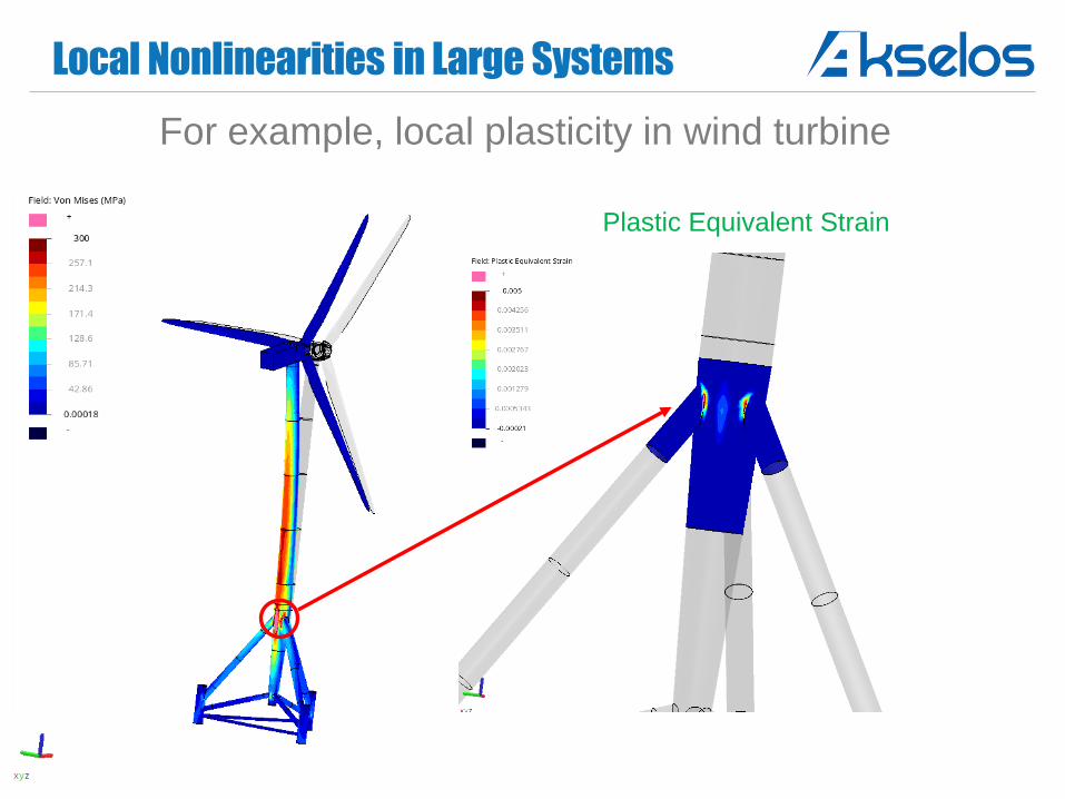
Local Nonlinearities in Large Systems
For example, local plasticity in wind turbine
Plastic Equivalent Strain
Nonlinear Analysis: Looking Ahead
Coupled SCRBE/FE works very well for localized
nonlinearities
In some systems nonlinearities are not localized, and
SCRBE/FE “degenerates” to global FE
Looking ahead: Strong interest in using model reduction
in the nonlinear regions as well…


![Multivariate Statistics [1em]Principal Component Analysis ...meier/teaching/cheming/4_multivariate.pdf · Principal Component Analysis (PCA) Goal: Dimensionality reduction. We have](https://img.pdfslide.us/doc/110x75/5e80b49cd82bd2127764cf4d/multivariate-statistics-1emprincipal-component-analysis-meierteachingcheming4.jpg)