Embed Size (px)
Citation preview
Auto-Tuning Algorithm for
Circulators based on Eigenvalue
Adjustments
Thomas Lingel
Th. Lingel Slide 2
• Circulator Magnetic components
• Permanent Magnet Materials and
Magnetization/Calibration Process
• Magnetizer Overview
• Common Tuning Approach
• Eigenvalues and Eigenvectors of Junction Circulators
• Auto-Tuning Algorithm
• Summary
Outline
Th. Lingel Slide 3
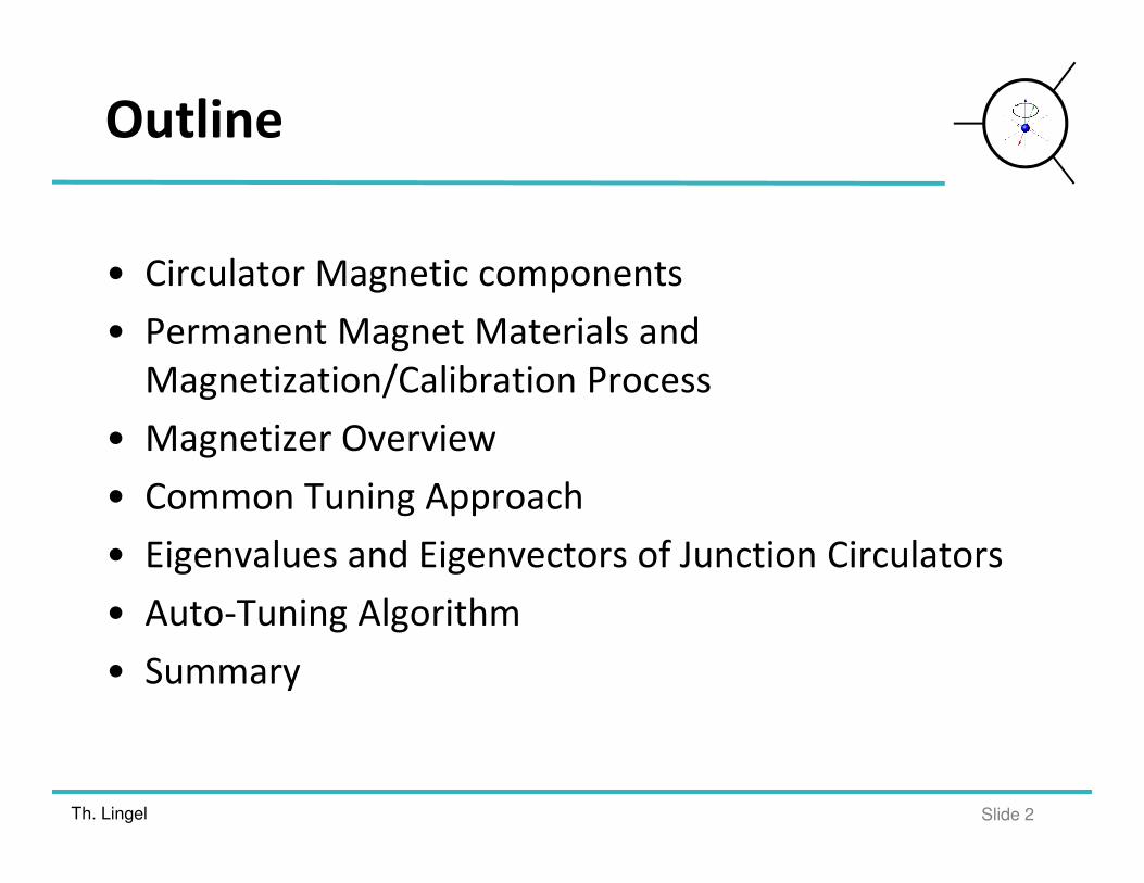
Circulator Operation
• Non-reciprocal behavior is based on elements of permeability
tensor,
• For above resonance devices the center frequency is adjusted
with the Magneto-Static Bias Field and requires very accurate
calibration
adjustedH i
r
−
=
100
0
0
µκ
κµ
µ j
j
P
t
sm Mπγω 4=
22
0
01ωω
ωωµ
−+= m
22
0 ωω
ωωκ
−= m
iHγω =0
E-Field Pattern
Th. Lingel Slide 4
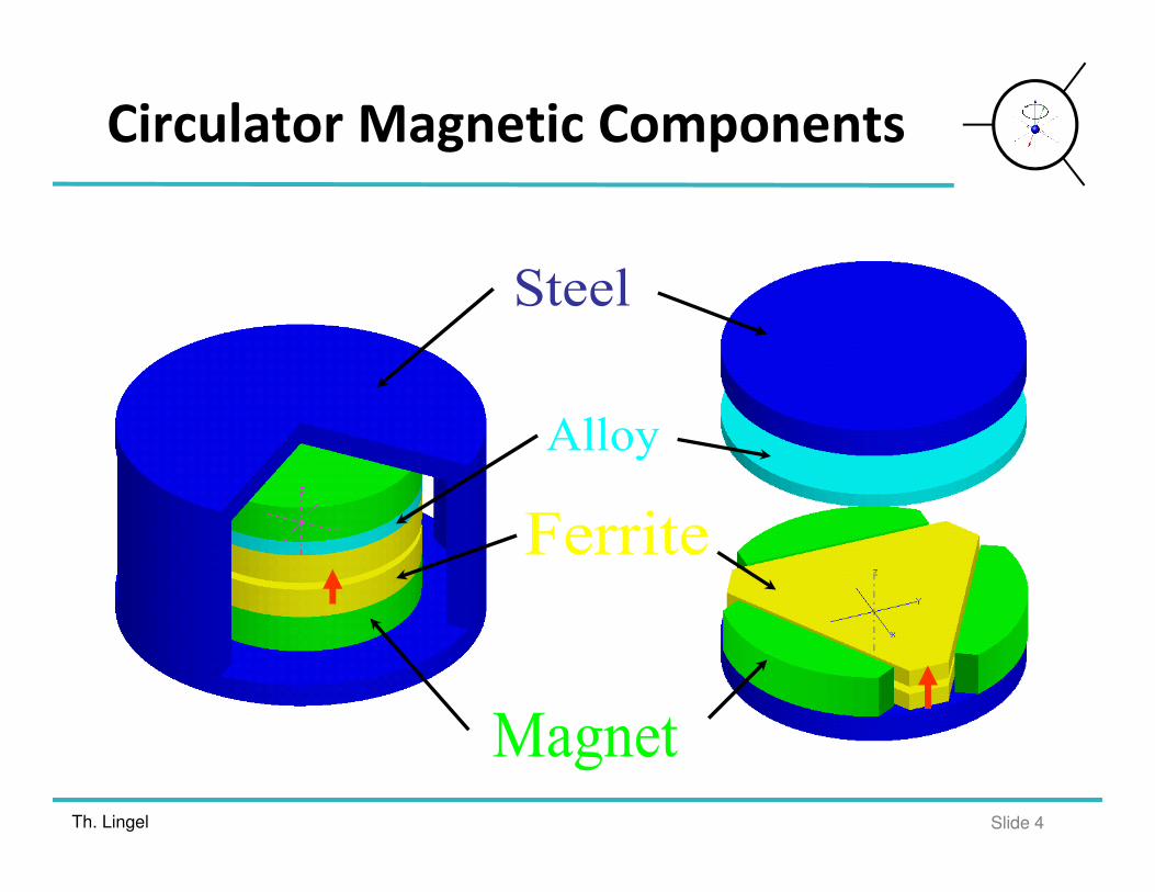
Circulator Magnetic Components
Th. Lingel Slide 5
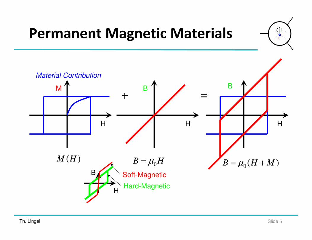
Permanent Magnetic Materials
H
B
HB 0µ=
B
H
)(0 MHB += µ
M
H
)(HM
Material Contribution
Soft-Magnetic
Hard-Magnetic
B
H
+ =
Th. Lingel Slide 6
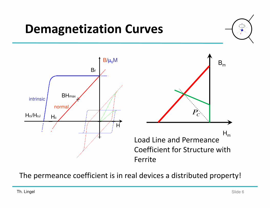
Demagnetization Curves
B/µ0M
H
HcHci/HcJ
Br
BHmaxintrinsic
normal
Bm
Hm
CP
Load Line and Permeance
Coefficient for Structure with
Ferrite
The permeance coefficient is in real devices a distributed property!
Th. Lingel Slide 7
Calibration of Permanent Magnets
B/µ0M
H
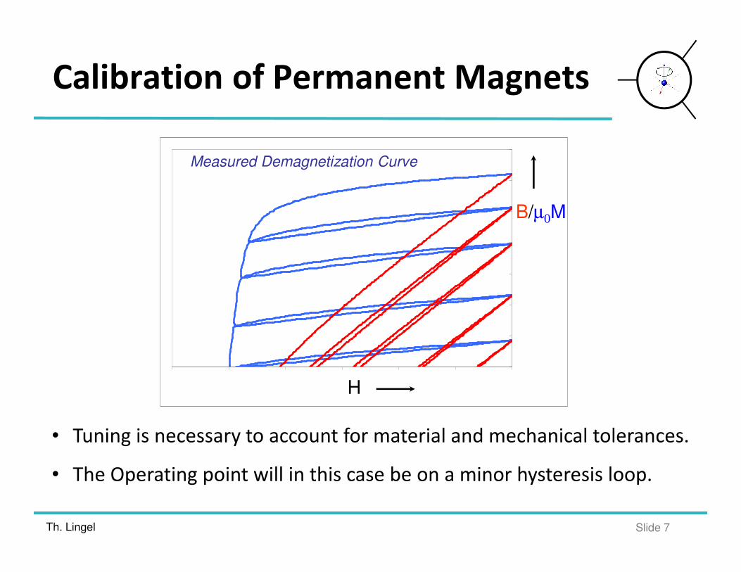
Measured Demagnetization Curve
• Tuning is necessary to account for material and mechanical tolerances.
• The Operating point will in this case be on a minor hysteresis loop.
Th. Lingel Slide 8
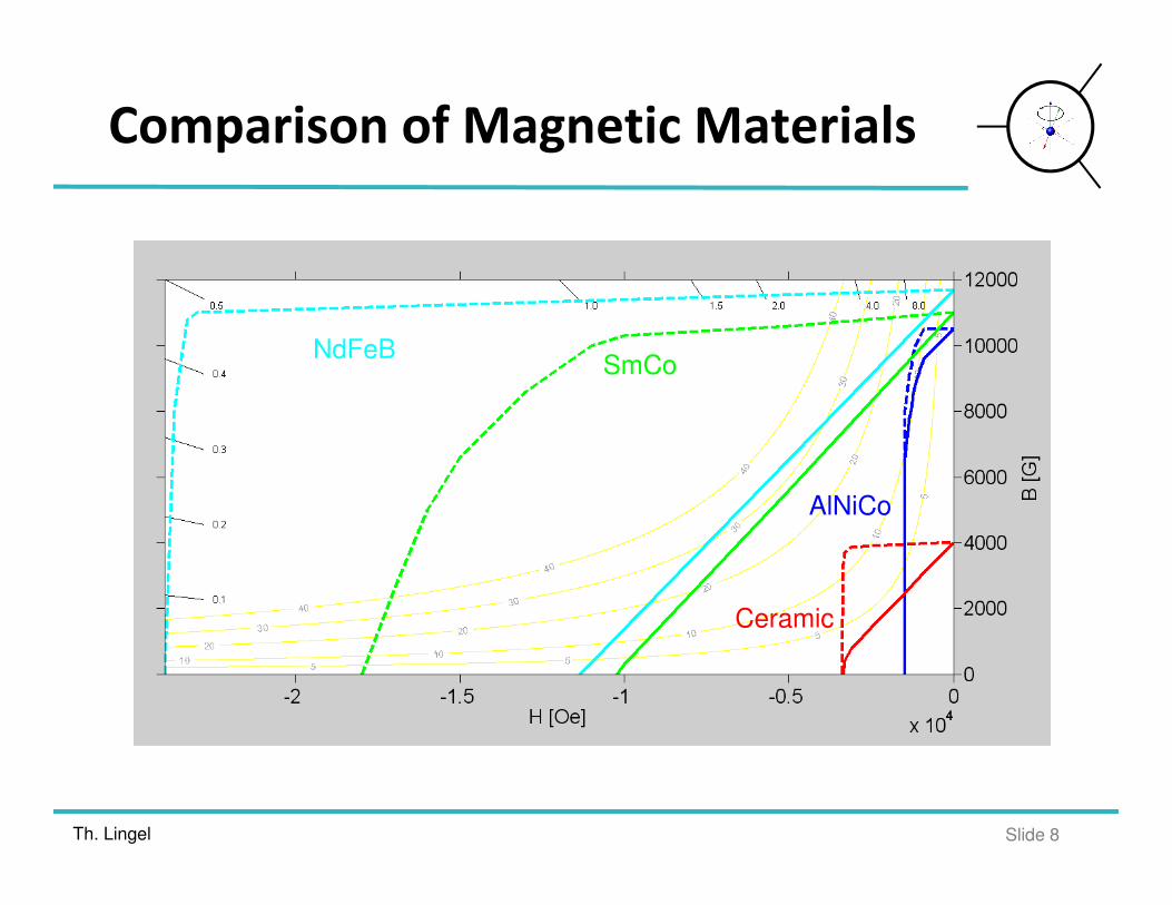
Comparison of Magnetic Materials
NdFeBSmCo
Ceramic
AlNiCo
Th. Lingel Slide 9
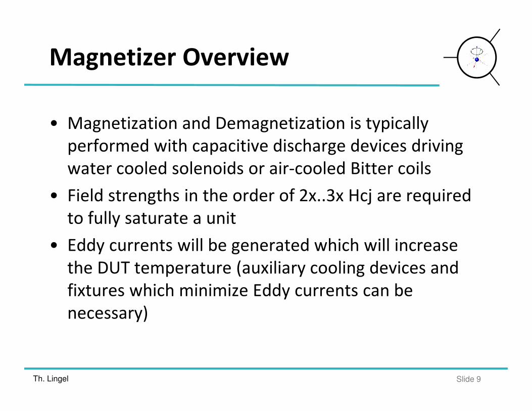
• Magnetization and Demagnetization is typically
performed with capacitive discharge devices driving
water cooled solenoids or air-cooled Bitter coils
• Field strengths in the order of 2x..3x Hcj are required
to fully saturate a unit
• Eddy currents will be generated which will increase
the DUT temperature (auxiliary cooling devices and
fixtures which minimize Eddy currents can be
necessary)
Magnetizer Overview
Th. Lingel Slide 10
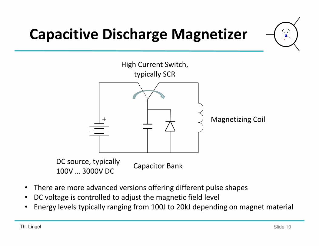
Capacitive Discharge Magnetizer
+
DC source, typically
100V … 3000V DCCapacitor Bank
Magnetizing Coil
High Current Switch,
typically SCR
• There are more advanced versions offering different pulse shapes
• DC voltage is controlled to adjust the magnetic field level
• Energy levels typically ranging from 100J to 20kJ depending on magnet material
Th. Lingel Slide 11
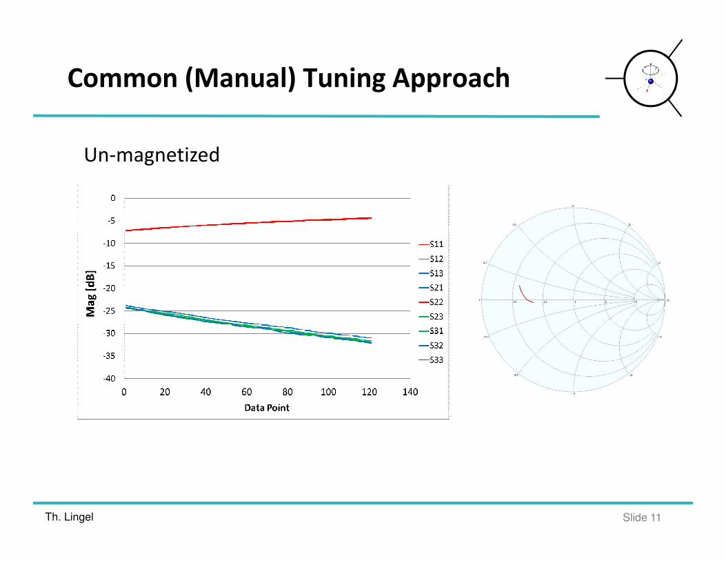
Common (Manual) Tuning Approach
Un-magnetized
Th. Lingel Slide 12
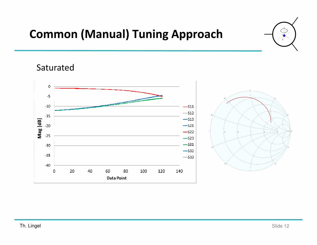
Common (Manual) Tuning Approach
Saturated
Th. Lingel Slide 13
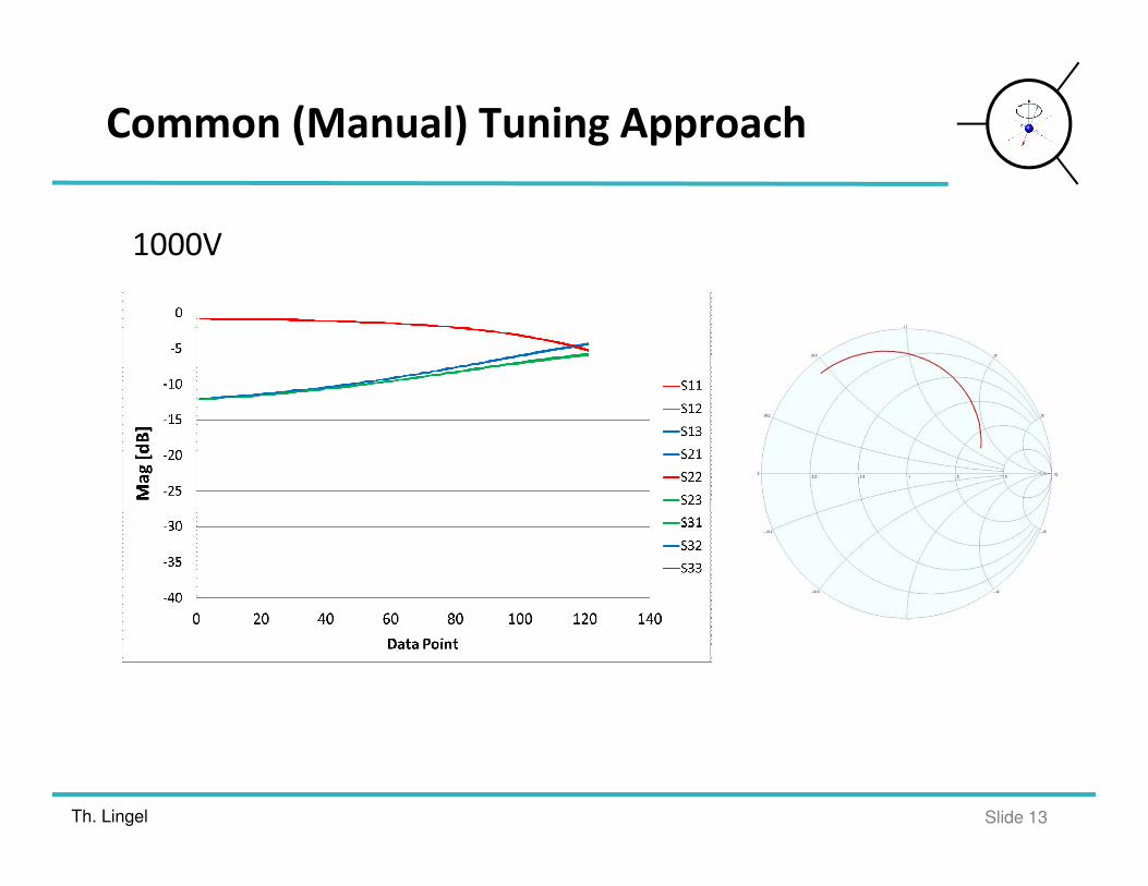
Common (Manual) Tuning Approach
1000V
Th. Lingel Slide 14
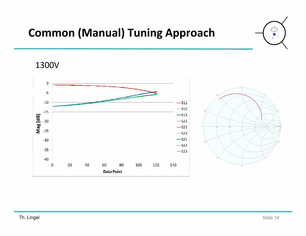
Common (Manual) Tuning Approach
1300V
Th. Lingel Slide 15
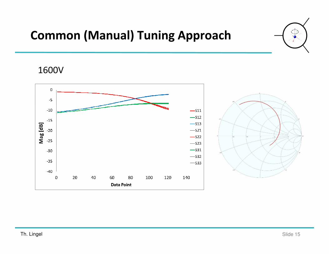
Common (Manual) Tuning Approach
1600V

Th. Lingel Slide 16
Common (Manual) Tuning Approach
1700V
Th. Lingel Slide 17
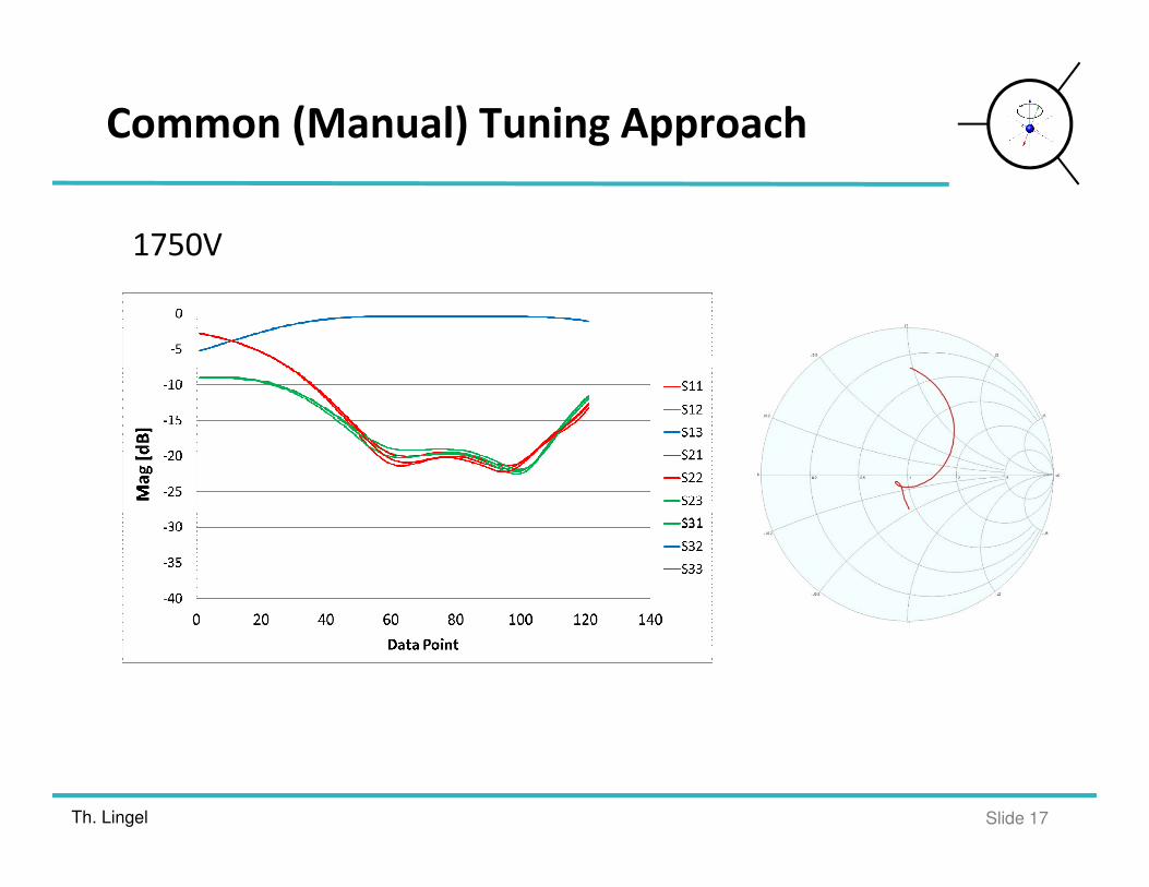
Common (Manual) Tuning Approach
1750V
Th. Lingel Slide 18
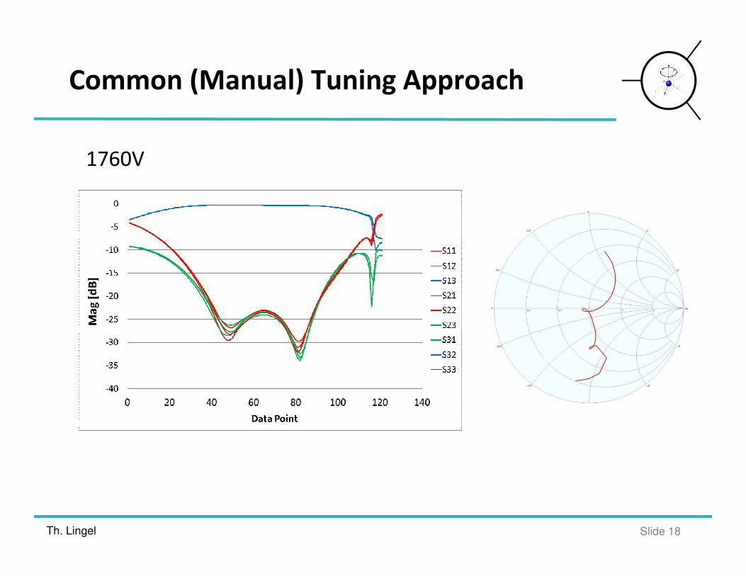
Common (Manual) Tuning Approach
1760V
Th. Lingel Slide 19
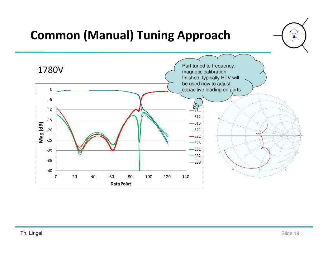
Common (Manual) Tuning Approach
1780VPart tuned to frequency,
magnetic calibration
finished, typically RTV will
be used now to adjust
capacitive loading on ports
Th. Lingel Slide 20
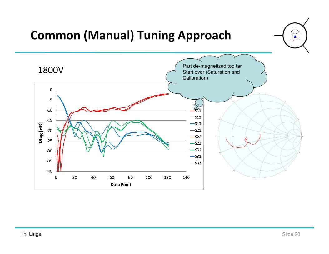
Common (Manual) Tuning Approach
1800VPart de-magnetized too far
Start over (Saturation and
Calibration)
Th. Lingel Slide 21
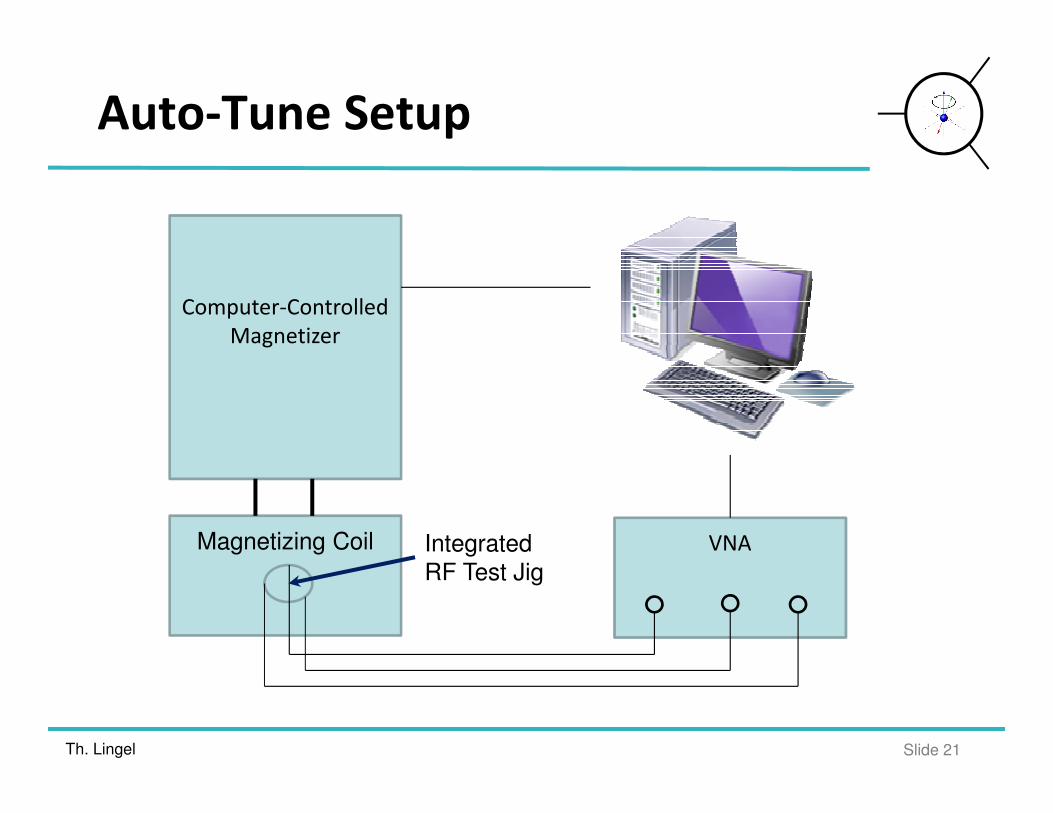
Auto-Tune Setup
Computer-Controlled
Magnetizer
Magnetizing Coil
Magnetizing Coil VNAIntegrated
RF Test Jig
Th. Lingel Slide 22
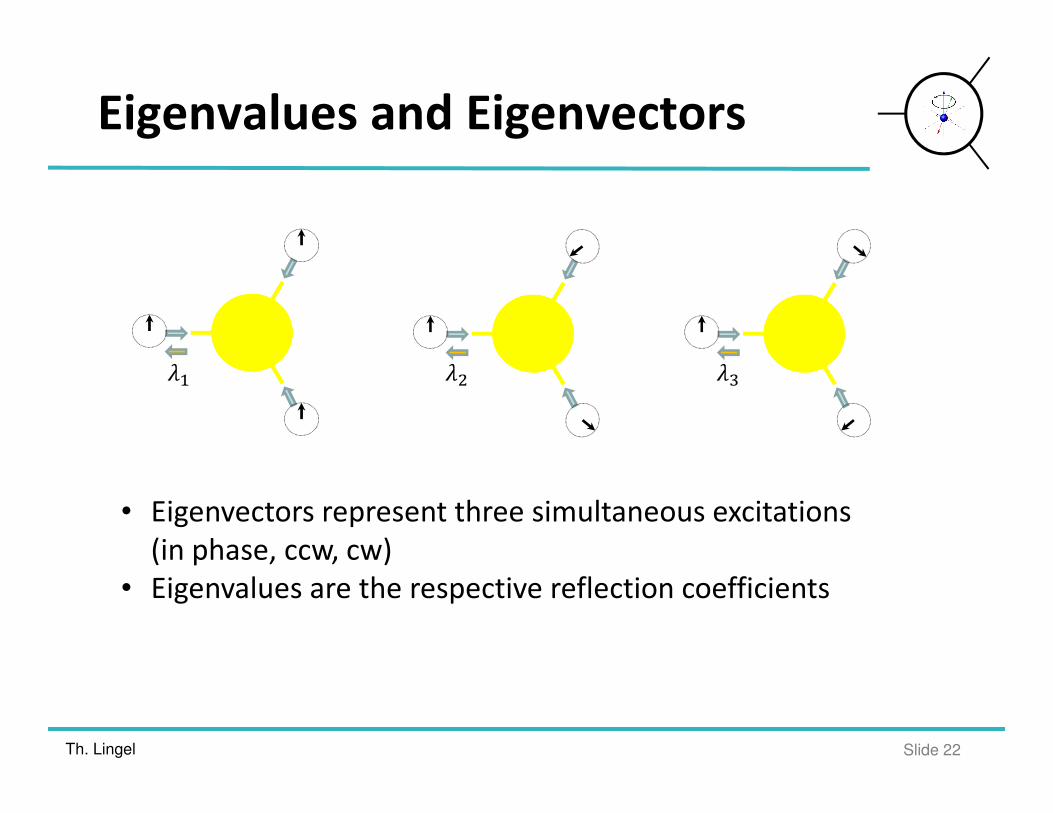
Eigenvalues and Eigenvectors
�� �� ��
• Eigenvectors represent three simultaneous excitations
(in phase, ccw, cw)
• Eigenvalues are the respective reflection coefficients
Th. Lingel Slide 23
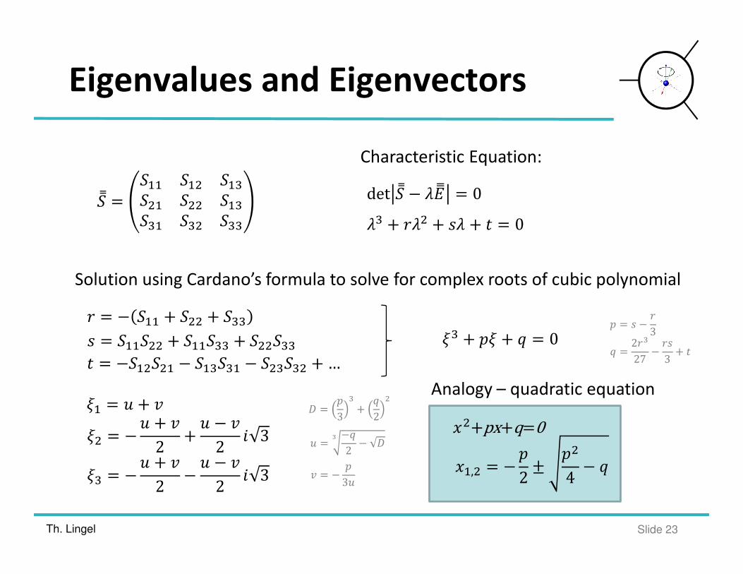
Eigenvalues and Eigenvectors
�̿ =
��� ��� ���
��� ��� ���
��� ��� ���
Characteristic Equation:
det �̿ − �� = 0
�� + ��� + �� + � = 0
Solution using Cardano’s formula to solve for complex roots of cubic polynomial
� = − ��� + ��� + ���
� = ������ + ������ + ������
� = −������ − ������ − ������ + …
�� + �� + � = 0
�� = � + �
�� = −� + �
2+
� − �
2� 3
�� = −� + �
2−
� − �
2� 3
��+px+q=0
��,� = −�
2±
��
4− �
Analogy – quadratic equation
� = � −�
3
� =2��
27−
��
3+ �
� =−�
2− %
&
� = −�
3�
% =�
3
�
+�
2
�
Th. Lingel Slide 24
Eigenvalue Calculation Symmetric Case
�̿ =
��� ��� ���
��� ��� ���
��� ��� ���
��
��
��
=
1 1 1
1 exp()4
3*) exp()
2
3*)
1 exp()2
3*) exp()
4
3*)
���������
���������
=1
3
1 1 1
1 exp()2
3*) exp()
4
3*)
1 exp()4
3*) exp()
2
3*)
������
,� = ∠�� − ∠��
,� = ∠�� − ∠��
• In the lossless case the magnitude of the Eigenvalues is 1
• Only the difference of the Eigenvalue angle needs to be considered
3x3 complex S-parameter matrix with 18 numbers is reduced to two numbers !
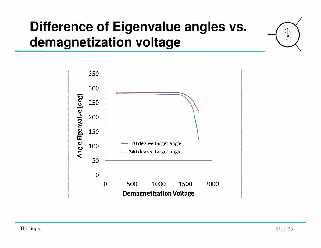
Th. Lingel Slide 25
Difference of Eigenvalue angles vs.
demagnetization voltage
Th. Lingel Slide 26
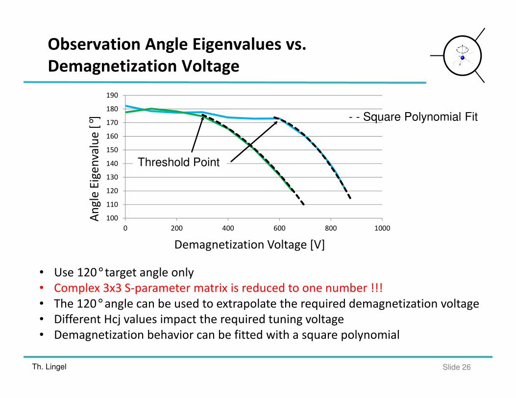
Observation Angle Eigenvalues vs.
Demagnetization Voltage
100
110
120
130
140
150
160
170
180
190
0 200 400 600 800 1000
An
gle
Eig
en
valu
e [°]
Demagnetization Voltage [V]
• Use 120°target angle only
• Complex 3x3 S-parameter matrix is reduced to one number !!!
• The 120°angle can be used to extrapolate the required demagnetization voltage
• Different Hcj values impact the required tuning voltage
• Demagnetization behavior can be fitted with a square polynomial
- - Square Polynomial Fit
Threshold Point
Th. Lingel Slide 27
• Place completely assembled unit into test-jig, residing in
magnetizing fixture
• Saturate unit
• Demagnetize until threshold is reached
• Perform two additional demagnetization steps to be able to
fit square polynomial
• Extrapolate to target angle of 125°
• Use last three data points and extrapolate to target angle of
120°
• Algorithm can be applied at center frequency or a mean value
across the operating frequency band
Auto-Tuning Algorithm
Th. Lingel Slide 28
• A robust algorithm for auto-tuning of circulators is presented
for the first time
• The 3x3 complex S-Parameter matrix is reduced to a single
number
• The angle difference of two Eigenvalues vs. demagnetization
voltage can be fitted with a square polynomial and can be
used to extrapolate to the target of 120°
• The algorithm is in particular useful for high volume
applications
Summary