481 lecture20

Whites, EE 481/581 Lecture 20 Page 1 of 7

© 2015 Keith W. Whites

Lecture 20: Transmission (ABCD) Matrix. Concerning the equivalent port representations of networks we’ve seen in this course:

1. Z parameters are useful for series connected networks, 2. Y parameters are useful for parallel connected networks, 3. S parameters are useful for describing interactions of

voltage and current waves with a network. There is another set of network parameters particularly suited for cascading two-port networks. This set is called the ABCD matrix or, equivalently, the transmission matrix. Consider this two-port network (Fig. 4.11a):

1V+

-

A B

C D

1I

2V+

-

2I

Unlike in the definition used for Z and Y parameters, notice that

2I is directed away from the port. This is an important point and we’ll discover the reason for it shortly. The ABCD matrix is defined as

1 2

1 2

V VA B

I IC D

(4.69),(1)


It is easy to show that

2

1

2 0I

VA

V

, 2

1

2 0V

VB

I

2

1

2 0I

IC

V

, 2

1

2 0V

ID

I

Note that not all of these parameters have the same units.

The usefulness of the ABCD matrix is that cascaded two-port networks can be characterized by simply multiplying their ABCD matrices. Nice!

To see this, consider the following two-port networks:

1V1 1

1 1

A B

C D

1I

2V

2I

2V 2 2

2 2

A B

C D

2I

3V

3I

In matrix form

1 1 1 2

1 1 1 2

V A B V

I C D I

(4.70a),(2)

and 32 2 2

32 22

VV A B

IC DI

(3)

When these two-ports are cascaded,


2V +

-

2 2

2 2

A B

C D

2I

3V+

-

3I

1V+

-

1 1

1 1

A B

C D

1I

2V+

-

2I

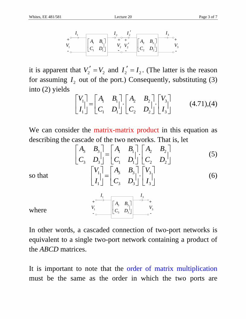
it is apparent that 2 2V V and 2 2I I . (The latter is the reason for assuming 2I out of the port.) Consequently, substituting (3) into (2) yields

31 1 1 2 2

31 1 1 2 2

VV A B A B

II C D C D

(4.71),(4)

We can consider the matrix-matrix product in this equation as describing the cascade of the two networks. That is, let

3 3 1 1 2 2

3 3 1 1 2 2

A B A B A B

C D C D C D

(5)

so that 3 3 31

3 3 31

A B VV

C D II

(6)

where

1V+

-

3 3

3 3

A B

C D

1I

3V+

-

3I

In other words, a cascaded connection of two-port networks is equivalent to a single two-port network containing a product of the ABCD matrices. It is important to note that the order of matrix multiplication must be the same as the order in which the two ports are


arranged in the circuit from signal input to output. Matrix multiplication is not commutative, in general. That is,

A B B A .

Text example 4.6 shows the derivation of the ABCD parameters for a series (i.e., “floating”) impedance, which is the first entry in Table 4.1 on p. 190 of the text. In your homework, you’ll derive the ABCD parameters for the next three entries in the table. In the following example, we’ll derive the last entry in this table.

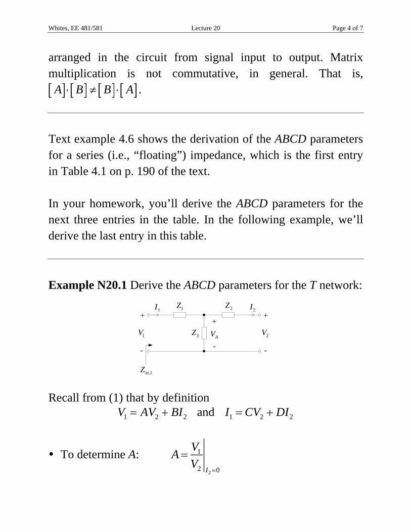
Example N20.1 Derive the ABCD parameters for the T network:

1V

+

-

1Z

2V

+

-

3Z

2Z1I 2I

+

-AV

in,1Z

Recall from (1) that by definition 1 2 2V AV BI and 1 2 2I CV DI

To determine A: 2

1

2 0I

VA

V


we need to open-circuit port 2 so that 2 0I . Hence,

31 2

1 3A

ZV V V

Z Z

which yields, 2

1 1

2 30

1I

V ZA

V Z

To determine B: 2

1

2 0V

VB

I

we need to short-circuit port 2 so that 2 0V . Then, using current division:

32 1

2 3

ZI I

Z Z

Substituting this into the expression for B above we find

2

in,1 02

1 2 21 2 3

1 3 30

1 1

V

V

Z

V Z ZB Z Z Z

I Z Z

1 2 21 2 3

3 3

1Z Z Z

Z Z ZZ Z

2 3 3 21 21

3 2 3 3

Z Z Z ZZ ZZ

Z Z Z Z

Therefore, 1 21 2

3

Z ZB Z Z

Z


To determine C: 2

1

2 0I

IC

V

we need to open-circuit port 2, from which we find 1 3 2AV I Z V

Therefore, 2

1

2 30

1

I

IC

V Z

To determine D: 2

1

2 0V

ID

I

we need to short-circuit port 2. Using current division, as above,

32 1

2 3

ZI I

Z Z

Therefore, 2

1 2

2 30

1V

I ZD

I Z

These ABCD parameters agree with those listed in the last entry of Table 4.1.

Properties of ABCD parameters

As shown on p. 191 of the text, the ABCD parameters can be expressed in terms of the Z parameters. (Actually, there are


interrelationships between all the network parameters, which are conveniently listed in Table 4.2 on p. 192.) From this relationship, we can show that for a reciprocal network

Det 1A B

C D

or 1AD BC

If the network is lossless, there are no really outstanding features of the ABCD matrix. Rather, using the relationship to the Z parameters we can see that if the network is lossless, then

From (4.73a): 11

21

ZA A

Z real

From (4.73b): 11 22 12 21

21

Z Z Z ZB B

Z

imaginary

From (4.73c): 21

1C C

Z imaginary

From (4.73d): 22

21

ZD D

Z real

In other words, the diagonal elements are real while the off-diagonal elements are imaginary for an ABCD matrix representation of a lossless network.

Engineering

481 lecture20