Embed Size (px)
Citation preview


… may be sitting right in your classroom! Everyone of your students has the potential to make adifference. And realizing that potential startsright here, in your course.
When students succeed in your course—whenthey stay on-task and make the breakthrough thatturns confusion into confidence—they areempowered to realize the possibilities for great-ness that lie within each of them. We know your goal is to create an envi-ronment where students reach their full potential and experience theexhilaration of academic success that will last them a lifetime. WileyPLUScan help you reach that goal.
WileyPLUS is an online suite of resources—including the complete text—that will help your students:
• come to class better prepared for your lectures• get immediate feedback and context-sensitive help on assignments
and quizzes• track their progress throughout the course
of students surveyed said it improved their understanding of the material.
The first person to invent a car that runs on water…
“I just wanted to say how much this program helped mein studying… I was able to actually see my mistakes andcorrect them. … I really think that other students shouldhave the chance to use WileyPLUS.”
Ashlee Krisko, Oakland University
*80%www.wiley.com/college/wileyplus

FOR INSTRUCTORS
FOR STUDENTS
of students surveyed said it made them better prepared for tests.76%
“It has been a great help,and I believe it has helpedme to achieve a bettergrade.”
Michael Morris,Columbia Basin College
**Based on a survey of 972 student users of WileyPLUS
WileyPLUS is built around the activities you perform in your class each day. With WileyPLUS you can:
Prepare & PresentCreate outstanding class presentationsusing a wealth of resources such as PowerPoint™ slides, image galleries,interactive simulations, and more.You can even add materials you havecreated yourself.
Create AssignmentsAutomate the assigning and grading ofhomework or quizzes by using the pro-vided question banks, or by writing yourown.
Track Student ProgressKeep track of your students' progressand analyze individual and overall classresults.
•A complete online version of your textand other study resources.
•Problem-solving help, instant grading,and feedback on your homework andquizzes.
•The ability to track your progress andgrades throughout the term.
For more information on what WileyPLUS can do to help you and your students reach their potential,please visit www.wiley.com/college/wileyplus.
Now Available with WebCT and Blackboard!
You have the potential to make a difference! WileyPLUS is a powerful online system packed with features to help you make the most
of your potential and get the best grade you can!
With WileyPLUS you get:

Introduction to Analog and Digital Communications

This page intentionally left blank
Introduction to Analog and Digital CommunicationsSecond Edition
Simon Haykin McMaster University, Hamilton, Ontario, Canada
Michael Moher Space-Time DSP, Ottawa, Ontario, Canada
JOHN WILEY & SONS, INC.
ASSOCIATE PUBLISHER Dan SayreSENIOR ACQUISITIONS EDITOR AND PROJECT MANAGER Catherine ShultzPROJECT EDITOR Gladys SotoMARKETING MANAGER Phyllis Diaz CerysEDITORIAL ASSISTANT Dana KellogSENIOR PRODUCTION EDITOR Lisa WojcikMEDIA EDITOR Stefanie LiebmanDESIGNER Hope MillerSENIOR ILLUSTRATION EDITOR Sigmund MalinowskiCOVER IMAGE © Photodisc/Getty Images
This book was set in Quark by Prepare Inc. and printed and bound by Hamilton Printing. The cover was printedby Phoenix Color Corp.
This book is printed on acid free paper.
Copyright © 2007 John Wiley & Sons, Inc. All rights reserved. No part of this publication may be reproduced,stored in a retrieval system, or transmitted in any form or by any means, electronic, mechanical, photocopying,recording, scanning, or otherwise, except as permitted under Sections 107 or 108 of the 1976 United States Copy-right Act, without either the prior written permission of the Publisher, or authorization through payment of theappropriate per-copy fee to the Copyright Clearance Center, Inc., 222 Rosewood Drive, Danvers, MA 01923,(978)750-8400, fax (978)646-8600, or on the web at www.copyright.com. Requests to the Publisher for per-mission should be addressed to the Permissions Department, John Wiley & Sons, Inc., 111 River Street, Hobo-ken, NJ 07030-5774, (201)7486011, fax (201)748-6008, or online at http://www.wiley.com/go/permissions.
To order books or for customer service please, call 1-800-CALL WILEY (225-5945).
ISBN-13 978-0-471-43222-7ISBN-10 0-471-43222-9
Printed in the United States of America
10 9 8 7 6 5 4 3 2 1
�

To the 20th Century pioneers in communications who, through their mathematical theories and ingenious devices,
have changed our planet into a global village

This page intentionally left blank
PREFACEAn introductory course on analog and digital communications is fundamental to the under-graduate program in electrical engineering. This course is usually offered at the junior level.Typically, it is assumed that the student has a background in calculus, electronics, signalsand systems, and possibly probability theory.
Bearing in mind the introductory nature of this course, a textbook recommended forthe course must be easy to read, accurate, and contain an abundance of insightful exam-ples, problems, and computer experiments. These objectives of the book are needed toexpedite learning the fundamentals of communication systems at an introductory level andin an effective manner. This book has been written with all of these objectives in mind.
Given the mathematical nature of communication theory, it is rather easy for thereader to lose sight of the practical side of communication systems. Throughout the book,we have made a special effort not to fall into this trap. We have done this by movingthrough the treatment of the subject in an orderly manner, always trying to keep the math-ematical treatment at an easy-to-grasp level and also pointing out practical relevance of thetheory wherever it is appropriate to do so.
Structural Philosophy of the Book
To facilitate and reinforce learning, the layout and format of the book have beenstructured to do the following:
• Provide motivation to read the book and learn from it.
• Emphasize basic concepts from a “systems” perspective and do so in an orderly manner.
• Wherever appropriate, include examples and computer experiments in each chapter to illus-trate application of the pertinent theory.
• Provide drill problems following the discussion of fundamental concepts to help the userof the book verify and master the concepts under discussion.
• Provide additional end-of-chapter problems, some of an advanced nature, to extend thetheory covered in the text.
Organization of the book
1. Motivation Before getting deeply involved in the study of analog and digital communi-cations, it is imperative that the user of the book be motivated to use the book and learnfrom it. To this end, Chapter 1 begins with a historical background of communication sys-tems and important applications of the subject.
2. Modulation Theory Digital communication has overtaken analog communications as thedominant form of communications. Although, indeed, these two forms of communicationswork in different ways, modulation theory is basic to them both. Moreover, it is easiest tounderstand this important subject by first covering its fundamental concepts applied to ana-log communications and then moving on to digital communications. Moreover, amplitudemodulation is simpler than angle modulation to present. One other highly relevant point isthe fact that to understand modulation theory, it is important that Fourier theory be mas-tered first. With these points in mind, Chapters 2 through 7 are organized as follows:
ix
x APPENDIX 1 � POWER RATIOS AND DECIBEL
• Chapter 2 is devoted to reviewing the Fourier representation of signals and systems.
• Chapters 3 and 4 are devoted to analog communications, with Chapter 3 covering ampli-tude modulation and Chapter 4 covering angle modulation.
• Chapter 5 on pulse modulation covers the concepts pertaining to the transition from ana-log to digital communications.
• Chapters 6 and 7 are devoted to digital communications, with Chapter 6 covering base-band data transmission and Chapter 7 covering band-pass data transmission.
3. Probability Theory and Signal Detection Just as Fourier analysis is fundamental to mod-ulation theory, probability theory is fundamental to signal detection and receiver performanceevaluation in the presence of additive noise. Since probability theory is not critical to theunderstanding of modulation, we have purposely delayed the review of probability theory,random signals, and noise until Chapter 8. Then, with a good understanding of modulationtheory applied to analog and digital communications and relevant concepts of probabilitytheory and probabilistic models at hand, the stage is set to revisit analog and digital com-munication receivers, as summarized here:
• Chapter 9 discusses noise in analog communications.
• Chapter 10 discusses noise in digital communications. Because analog and digital com-munications operate in different ways, it is natural to see some fundamental differencesin treating the effects of noise in these two chapters.
4. Noise The introductory study of analog and digital communications is completed in Chap-ter 11. This chapter illustrates the roles of modulation and noise in communication systemsby doing four things:
• First, the physical sources of noise, principally, thermal noise and shot noise, are described.
• Second, the metrics of noise figure and noise temperature are introduced.
• Third, how propagation affects the signal strength in satellite and terrestrial wireless com-munications is explained.
• Finally, we show how the signal strength and noise calculations may be combined to pro-vide an estimate of the signal-to-noise ratio, the fundamental figure of merit for commu-nication systems.
5. Theme Examples In order to highlight important practical applications of communicationtheory, theme examples are included wherever appropriate. The examples are drawn fromthe worlds of both analog and digital communications.
6. Appendices To provide back-up material for the text, eight appendices are included at theend of the book, which cover the following material in the order presented here:
• Power ratios and the decibel
• Fourier series
• Bessel functions
• The Q-function and its relationship to the error function
• Schwarz’s inequality
• Mathematical tables
Preface xi
• Matlab scripts for computer experiments to problems in Chapters 7–10
• Answers to drill problems
7. Footnotes, included throughout the book, are provided to help the interested reader to pur-sue selected references for learning advanced material.
8. Auxiliary Material The book is essentially self-contained. A glossary of symbols and abibliography are provided at the end of the book. As an aid to the teacher of the course usingthe book, a detailed Solutions Manual for all the problems, those within the text and thoseincluded at the end of chapters, will be made available through the publisher: John Wileyand Sons.
How to Use the Book
The book can be used for an introductory course on analog and digital communicationsin different ways, depending on the background of the students and the teaching interestsand responsibilities of the professors concerned. Here are two course models of how thismay be done:
COURSE MODEL A: FULL TWO-SEMESTER COURSE
(A.1) The first semester course on modulation theory consists of Chapters 2 through 7, inclu-sive.
(A.2) The second semester course on noise in communication systems consists of Chapters 8through 11, inclusive.
COURSE MODEL B: TWO SEMESTER COURSES, ONE ON ANALOG AND THE
OTHER ON DIGITAL
(B.1) The first course on analog communications begins with review material from Chapter 2on Fourier analysis, followed by Chapter 3 on amplitude modulation and Chapter 4 onangle modulation, then proceeds with a review of relevant parts of Chapter 8 on noise,and finally finishes with Chapter 9 on noise in analog communications.
(B.2) The second course on digital communications starts with Chapter 5 on pulse modulation,followed by Chapter 6 on baseband data transmission and Chapter 7 on digital modu-lation techniques, then proceeds with review of relevant aspects of probability theory inChapter 8, and finally finishes with Chapter 10 on noise in digital communications.
Simon HaykinAncaster, Ontario, Canada
Michael MoherOttawa, Ontario, Canada

This page intentionally left blank
xiii
ACKNOWLEDGEMENTSThe authors would like to express their deep gratitude to
• Lily Jiang, formerly of McMaster University for her help in performing many of thecomputer experiments included in the text.
• Wei Zhang, for all the help, corrections, and improvements she has made to the text.
They also wish to thank Dr. Stewart Crozier and Dr. Paul Guinand, both of the Commu-nications Research Centre, Ottawa, for their inputs on different parts of the book.
They are also indebted to Catherine Fields Shultz, Senior Acquisitions Editor andProduct Manager (Engineering and Computer Science) at John Wiley and Sons, Bill Zobristformerly of Wiley, and Lisa Wojcik, Senior Production Editor at Wiley, for their guidanceand dedication to the production of this book.
Last but by no means least, they are grateful to Lola Brooks, McMaster University,for her hard work on the preparation of the manuscript and related issues to the book.

This page intentionally left blank
xv
CONTENTS
Chapter 1 Introduction 1
1.1 Historical Background 1
1.2 Applications 4
1.3 Primary Resources and Operational Requirements 13
1.4 Underpinning Theories of Communication Systems 14
1.5 Concluding Remarks 16
Chapter 2 Fourier Representation of Signals and Systems 18
2.1 The Fourier Transform 19
2.2 Properties of the Fourier Transform 25
2.3 The Inverse Relationship Between Time and Frequency 39
2.4 Dirac Delta Function 42
2.5 Fourier Transforms of Periodic Signals 50
2.6 Transmission of Signals Through Linear Systems: ConvolutionRevisited 52
2.7 Ideal Low-pass Filters 60
2.8 Correlation and Spectral Density: Energy Signals 70
2.9 Power Spectral Density 79
2.10 Numerical Computation of the Fourier Transform 81
2.11 Theme Example: Twisted Pairs for Telephony 89
2.12 Summary and Discussion 90
Additional Problems 91
Advanced Problems 98
Chapter 3 Amplitude Modulation 100
3.1 Amplitude Modulation 101
3.2 Virtues, Limitations, and Modifications of Amplitude Modulation 113
3.3 Double Sideband-Suppressed Carrier Modulation 114
3.4 Costas Receiver 120
xvi APPENDIX 1 � POWER RATIOS AND DECIBEL
3.5 Quadrature-Carrier Multiplexing 121
3.6 Single-Sideband Modulation 123
3.7 Vestigial Sideband Modulation 130
3.8 Baseband Representation of Modulated Waves and Band-Pass Filters 137
3.9 Theme Examples 142
3.10 Summary and Discussion 147
Additional Problems 148
Advanced Problems 150
Chapter 4 Angle Modulation 152
4.1 Basic Definitions 153
4.2 Properties of Angle-Modulated Waves 154
4.3 Relationship between PM and FM Waves 159
4.4 Narrow-Band Frequency Modulation 160
4.5 Wide-Band Frequency Modulation 164
4.6 Transmission Bandwidth of FM Waves 170
4.7 Generation of FM Waves 172
4.8 Demodulation of FM Signals 174
4.9 Theme Example: FM Stereo Multiplexing 182
4.10 Summary and Discussion 184
Additional Problems 185
Advanced Problems 187
Chapter 5 Pulse Modulation: Transition from Analog to DigitalCommunications 190
5.1 Sampling Process 191
5.2 Pulse-Amplitude Modulation 198
5.3 Pulse-Position Modulation 202
5.4 Completing the Transition from Analog to Digital 203
5.5 Quantization Process 205
5.6 Pulse-Code Modulation 206
Contents xvii
5.7 Delta Modulation 211
5.8 Differential Pulse-Code Modulation 216
5.9 Line Codes 219
5.10 Theme Examples 220
5.11 Summary and Discussion 225
Additional Problems 226
Advanced Problems 228
Chapter 6 Baseband Data Transmission 231
6.1 Baseband Transmission of Digital Data 232
6.2 The Intersymbol Interference Problem 233
6.3 The Nyquist Channel 235
6.4 Raised-Cosine Pulse Spectrum 238
6.5 Baseband Transmission of M-ary Data 245
6.6 The Eye Pattern 246
6.7 Computer Experiment: Eye Diagrams for Binary and QuaternarySystems 249
6.8 Theme Example: Equalization 251
6.9 Summary and Discussion 256
Additional Problems 257
Advanced Problems 259
Chapter 7 Digital Band-Pass Modulation Techniques 262
7.1 Some Preliminaries 262
7.2 Binary Amplitude-Shift Keying 265
7.3 Phase-Shift Keying 270
7.4 Frequency-Shift Keying 281
7.5 Summary of Three Binary Signaling Schemes 289
7.6 Noncoherent Digital Modulation Schemes 291
7.7 M-ary Digital Modulation Schemes 295
7.8 Mapping of Digitally Modulated Waveforms onto Constellations of Signal Points 299
xviii APPENDIX 1 � POWER RATIOS AND DECIBEL
7.9 Theme Examples 302
7.10 Summary and Discussion 307
Additional Problems 309
Advanced Problems 310
Computer Experiments 312
Chapter 8 Random Signals and Noise 313
8.1 Probability and Random Variables 314
8.2 Expectation 326
8.3 Transformation of Random Variables 329
8.4 Gaussian Random Variables 330
8.5 The Central Limit Theorem 333
8.6 Random Processes 335
8.7 Correlation of Random Processes 338
8.8 Spectra of Random Signals 343
8.9 Gaussian Processes 347
8.10 White Noise 348
8.11 Narrowband Noise 352
8.12 Summary and Discussion 356
Additional Problems 357
Advanced Problems 361
Computer Experiments 363
Chapter 9 Noise in Analog Communications 364
9.1 Noise in Communication Systems 365
9.2 Signal-to-Noise Ratios 366
9.3 Band-Pass Receiver Structures 369
9.4 Noise in Linear Receivers Using Coherent Detection 370
9.5 Noise in AM Receivers Using Envelope Detection 373
9.6 Noise in SSB Receivers 377
9.7 Detection of Frequency Modulation (FM) 380
Contents xix
9.8 FM Pre-emphasis and De-emphasis 387
9.9 Summary and Discussion 390
Additional Problems 391
Advanced Problems 392
Computer Experiments 393
Chapter 10 Noise in Digital Communications 394
10.1 Bit Error Rate 395
10.2 Detection of a Single Pulse in Noise 396
10.3 Optimum Detection of Binary PAM in Noise 399
10.4 Optimum Detection of BPSK 405
10.5 Detection of QPSK and QAM in Noise 408
10.6 Optimum Detection of Binary FSK 414
10.7 Differential Detection in Noise 416
10.8 Summary of Digital Performance 418
10.9 Error Detection and Correction 422
10.10 Summary and Discussion 433
Additional Problems 434
Advanced Problems 435
Computer Experiments 436
Chapter 11 System and Noise Calculations 437
11.1 Electrical Noise 438
11.2 Noise Figure 442
11.3 Equivalent Noise Temperature 443
11.4 Cascade Connection of Two-Port Networks 445
11.5 Free-Space Link Calculations 446
11.6 Terrestrial Mobile Radio 451
11.7 Summary and Discussion 456
Additional Problems 457
Advanced Problems 458
xx APPENDIX 1 � POWER RATIOS AND DECIBEL
APPENDIX 1 POWER RATIOS AND DECIBEL 459
APPENDIX 2 FOURIER SERIES 460
APPENDIX 3 BESSEL FUNCTIONS 467
APPENDIX 4 THE Q-FUNCTION AND ITS RELATIONSHIP TO THE ERROR
FUNCTION 470
APPENDIX 5 SCHWARZ’S INEQUALITY 473
APPENDIX 6 MATHEMATICAL TABLES 475
APPENDIX 7 MATLAB SCRIPTS FOR COMPUTER EXPERIMENTS TO
PROBLEMS IN CHAPTERS 7-10 480
APPENDIX 8 ANSWERS TO DRILL PROBLEMS 488
GLOSSARY 495
BIBLIOGRAPHY 498
INDEX 501

1
1 This historical background is adapted from Haykin’s book (2001).
CHAPTER 1
INTRODUCTION
“To understand a science it is necessary to know its history”—Auguste Comte (1798–1857)
1.1 Historical Background
With this quotation from Auguste Comte in mind, we begin this introductory study ofcommunication systems with a historical account of this discipline that touches our dailylives in one way or another.1 Each subsection in this section focuses on some important andrelated events in the historical evolution of communication.
Telegraph
The telegraph was perfected by Samuel Morse, a painter. With the words “What hathGod wrought,” transmitted by Morse’s electric telegraph between Washington, D.C., andBaltimore, Maryland, in 1844, a completely revolutionary means of real-time, long-dis-tance communications was triggered. The telegraph, ideally suited for manual keying, is theforerunner of digital communications. Specifically, the Morse code is a variable-length codeusing an alphabet of four symbols: a dot, a dash, a letter space, and a word space; shortsequences represent frequent letters, whereas long sequences represent infrequent letters.
Radio
In 1864, James Clerk Maxwell formulated the electromagnetic theory of light and pre-dicted the existence of radio waves; the underlying set of equations bears his name. The exis-tence of radio waves was confirmed experimentally by Heinrich Hertz in 1887. In 1894,Oliver Lodge demonstrated wireless communication over a relatively short distance (150yards). Then, on December 12, 1901, Guglielmo Marconi received a radio signal at SignalHill in Newfoundland; the radio signal had originated in Cornwall, England, 1700 milesaway across the Atlantic. The way was thereby opened toward a tremendous broadeningof the scope of communications. In 1906, Reginald Fessenden, a self-educated academic,made history by conducting the first radio broadcast.
In 1918, Edwin H. Armstrong invented the superheterodyne radio receiver; to this day,almost all radio receivers are of this type. In 1933, Armstrong demonstrated another rev-olutionary concept—namely, a modulation scheme that he called frequency modulation(FM). Armstrong’s paper making the case for FM radio was published in 1936.
2 CHAPTER 1 � INTRODUCTION
Telephone
In 1875, the telephone was invented by Alexander Graham Bell, a teacher of the deaf.The telephone made real-time transmission of speech by electrical encoding and replicationof sound a practical reality. The first version of the telephone was crude and weak, enablingpeople to talk over short distances only. When telephone service was only a few years old,interest developed in automating it. Notably, in 1897, A. B. Strowger, an undertaker fromKansas City, Missouri, devised the automatic step-by-step switch that bears his name. Ofall the electromechanical switches devised over the years, the Strowger switch was the mostpopular and widely used.
Electronics
In 1904, John Ambrose Fleming invented the vacuum-tube diode, which paved theway for the invention of the vacuum-tube triode by Lee de Forest in 1906. The discoveryof the triode was instrumental in the development of transcontinental telephony in 1913and signaled the dawn of wireless voice communications. Indeed, until the invention andperfection of the transistor, the triode was the supreme device for the design of electronicamplifiers.
The transistor was invented in 1948 by Walter H. Brattain, John Bardeen, and WilliamShockley at Bell Laboratories. The first silicon integrated circuit (IC) was produced byRobert Noyce in 1958. These landmark innovations in solid-state devices and integratedcircuits led to the development of very-large-scale integrated (VLSI) circuits and single-chip microprocessors, and with them the nature of signal processing and the telecommu-nications industry changed forever.
Television
The first all-electronic television system was demonstrated by Philo T. Farnsworth in1928, and then by Vladimir K. Zworykin in 1929. By 1939, the British Broadcasting Cor-poration (BBC) was broadcasting television on a commercial basis.
Digital Communications
In 1928, Harry Nyquist published a classic paper on the theory of signal transmis-sion in telegraphy. In particular, Nyquist developed criteria for the correct reception oftelegraph signals transmitted over dispersive channels in the absence of noise. Much ofNyquist’s early work was applied later to the transmission of digital data over dispersivechannels.
In 1937, Alex Reeves invented pulse-code modulation (PCM) for the digital encod-ing of speech signals. The technique was developed during World War II to enable theencryption of speech signals; indeed, a full-scale, 24-channel system was used in the fieldby the United States military at the end of the war. However, PCM had to await the dis-covery of the transistor and the subsequent development of large-scale integration of cir-cuits for its commercial exploitation.
The invention of the transistor in 1948 spurred the application of electronics toswitching and digital communications. The motivation was to improve reliability, increasecapacity, and reduce cost. The first call through a stored-program system was placed inMarch 1958 at Bell Laboratories, and the first commercial telephone service with digitalswitching began in Morris, Illinois, in June 1960. The first T-1 carrier system transmissionwas installed in 1962 by Bell Laboratories.
1.1 Historical Background 3
In 1943, D. O. North devised the matched filter for the optimum detection of a knownsignal in additive white noise. A similar result was obtained in 1946 independently byJ. H. Van Vleck and D. Middleton, who coined the term matched filter.
In 1948, the theoretical foundations of digital communications were laid by ClaudeShannon in a paper entitled “A Mathematical Theory of Communication.” Shannon’spaper was received with immediate and enthusiastic acclaim. It was perhaps this responsethat emboldened Shannon to amend the title of his paper to “The Mathematical Theoryof Communications” when it was reprinted a year later in a book co-authored with War-ren Weaver. It is noteworthy that prior to the publication of Shannon’s 1948 classic paper,it was believed that increasing the rate of information transmission over a channel wouldincrease the probability of error. The communication theory community was taken by sur-prise when Shannon proved that this was not true, provided the transmission rate wasbelow the channel capacity.
Computer Networks
During the period 1943 to 1946, the first electronic digital computer, called theENIAC, was built at the Moore School of Electrical Engineering of the University ofPennsylvania under the technical direction of J. Presper Eckert, Jr., and John W. Mauchly.However, John von Neumann’s contributions were among the earliest and most funda-mental to the theory, design, and application of digital computers, which go back to thefirst draft of a report written in 1945. Computers and terminals started communicatingwith each other over long distances in the early 1950s. The links used were initiallyvoice-grade telephone channels operating at low speeds (300 to 1200 b/s). Various fac-tors have contributed to a dramatic increase in data transmission rates; notable amongthem are the idea of adaptive equalization, pioneered by Robert Lucky in 1965, and effi-cient modulation techniques, pioneered by G. Ungerboeck in 1982. Another idea widelyemployed in computer communications is that of automatic repeat-request (ARQ). TheARQ method was originally devised by H. C. A. van Duuren during World War II andpublished in 1946. It was used to improve radio-telephony for telex transmission overlong distances.
From 1950 to 1970, various studies were made on computer networks. However,the most significant of them in terms of impact on computer communications was theAdvanced Research Projects Agency Network (ARPANET), first put into service in 1971.The development of ARPANET was sponsored by the Advanced Research Projects Agencyof the U. S. Department of Defense. The pioneering work in packet switching was done onARPANET. In 1985, ARPANET was renamed the Internet. The turning point in the evo-lution of the Internet occurred in 1990 when Tim Berners-Lee proposed a hypermedia soft-ware interface to the Internet, which he named the World Wide Web. In the space of onlyabout two years, the Web went from nonexistence to worldwide popularity, culminatingin its commercialization in 1994. We may explain the explosive growth of the Internet byoffering these reasons:
� Before the Web exploded into existence, the ingredients for its creation were alreadyin place. In particular, thanks to VLSI, personal computers (PCs) had already becomeubiquitous in homes throughout the world, and they were increasingly equipped withmodems for interconnectivity to the outside world.
� For about two decades, the Internet had grown steadily (albeit within a confinedcommunity of users), reaching a critical threshold of electronic mail and file transfer.
� Standards for document description and transfer, hypertext markup language(HTML), and hypertext transfer protocol (HTTP) had been adopted.
4 CHAPTER 1 � INTRODUCTION
Thus, everything needed for creating the Web was already in place except for two criticalingredients: a simple user interface and a brilliant service concept.
Satellite Communications
In 1955, John R. Pierce proposed the use of satellites for communications. This pro-posal was preceded, however, by an earlier paper by Arthur C. Clark that was published in1945, also proposing the idea of using an Earth-orbiting satellite as a relay point for com-munication between two Earth stations. In 1957, the Soviet Union launched Sputnik I, whichtransmitted telemetry signals for 21 days. This was followed shortly by the launching ofExplorer I by the United States in 1958, which transmitted telemetry signals for about fivemonths. A major experimental step in communications satellite technology was taken withthe launching of Telstar I from Cape Canaveral on July 10, 1962. The Telstar satellite wasbuilt by Bell Laboratories, which had acquired considerable knowledge from pioneeringwork by Pierce. The satellite was capable of relaying TV programs across the Atlantic; thiswas made possible only through the use of maser receivers and large antennas.
Optical Communications
The use of optical means (e.g., smoke and fire signals) for the transmission of infor-mation dates back to prehistoric times. However, no major breakthrough in optical com-munications was made until 1966, when K. C. Kao and G. A. Hockham of StandardTelephone Laboratories, U. K., proposed the use of a clad glass fiber as a dielectric wave-guide. The laser (an acronym for light amplification by stimulated emission of radiation)had been invented and developed in 1959 and 1960. Kao and Hockham pointed out that(1) the attenuation in an optical fiber was due to impurities in the glass, and (2) the intrin-sic loss, determined by Rayleigh scattering, is very low. Indeed, they predicted that a lossof 20 dB/km should be attainable. This remarkable prediction, made at a time when thepower loss in a glass fiber was about 1000 dB/km, was to be demonstrated later. Nowa-days, transmission losses as low as 0.1 dB/km are achievable.
The spectacular advances in microelectronics, digital computers, and lightwave sys-tems that we have witnessed to date, and that will continue into the future, are all respon-sible for dramatic changes in the telecommunications environment. Many of these changesare already in place, and more changes will occur over time.
1.2 Applications
The historical background of Section 1.1 touches many of the applications of communi-cation systems, some of which are exemplified by the telegraph that has come and gone,while others exemplified by the Internet are of recent origin. In what follows, we will focuson radio, communication networks exemplified by the telephone, and the Internet, whichdominate the means by which we communicate in one of two basic ways or both, as sum-marized here:
� Broadcasting, which involves the use of a single powerful transmitter and numerousreceivers that are relatively inexpensive to build. In this class of communication sys-tems, information-bearing signals flow only in one direction, from the transmitter toeach of the receivers out there in the field.
� Point-to-point communications, in which the communication process takes placeover a link between a single transmitter and a single receiver. In this second class ofcommunication systems, there is usually a bidirectional flow of information-bearing
1.2 Applications 5
Source ofinformation
User ofinformationEstimate of
messagesignal
Transmitter
Channel
Information-bearing(message)
signal
Communication System
Transmittedsignal
Receivedsignal
Receiver
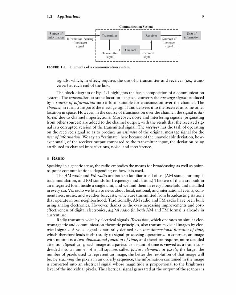
FIGURE 1.1 Elements of a communication system.
signals, which, in effect, requires the use of a transmitter and receiver (i.e., trans-ceiver) at each end of the link.
The block diagram of Fig. 1.1 highlights the basic composition of a communicationsystem. The transmitter, at some location in space, converts the message signal producedby a source of information into a form suitable for transmission over the channel. Thechannel, in turn, transports the message signal and delivers it to the receiver at some otherlocation in space. However, in the course of transmission over the channel, the signal is dis-torted due to channel imperfections. Moreover, noise and interfering signals (originatingfrom other sources) are added to the channel output, with the result that the received sig-nal is a corrupted version of the transmitted signal. The receiver has the task of operatingon the received signal so as to produce an estimate of the original message signal for theuser of information. We say an “estimate” here because of the unavoidable deviation, how-ever small, of the receiver output compared to the transmitter input, the deviation beingattributed to channel imperfections, noise, and interference.
� RADIO
Speaking in a generic sense, the radio embodies the means for broadcasting as well as point-to-point communications, depending on how it is used.
The AM radio and FM radio are both so familiar to all of us. (AM stands for ampli-tude modulation, and FM stands for frequency modulation.) The two of them are built inan integrated form inside a single unit, and we find them in every household and installedin every car. Via radio we listen to news about local, national, and international events, com-mentaries, music, and weather forecasts, which are transmitted from broadcasting stationsthat operate in our neighborhood. Traditionally, AM radio and FM radio have been builtusing analog electronics. However, thanks to the ever-increasing improvements and cost-effectiveness of digital electronics, digital radio (in both AM and FM forms) is already incurrent use.
Radio transmits voice by electrical signals. Television, which operates on similar elec-tromagnetic and communication-theoretic principles, also transmits visual images by elec-trical signals. A voice signal is naturally defined as a one-dimensional function of time,which therefore lends itself readily to signal-processing operations. In contrast, an imagewith motion is a two-dimensional function of time, and therefore requires more detailedattention. Specifically, each image at a particular instant of time is viewed as a frame sub-divided into a number of small squares called picture elements or pixels; the larger thenumber of pixels used to represent an image, the better the resolution of that image willbe. By scanning the pixels in an orderly sequence, the information contained in the imageis converted into an electrical signal whose magnitude is proportional to the brightnesslevel of the individual pixels. The electrical signal generated at the output of the scanner is
6 CHAPTER 1 � INTRODUCTION
Earth
Earthtransmitting
station
Earthreceiving
station
Downlink
Uplink
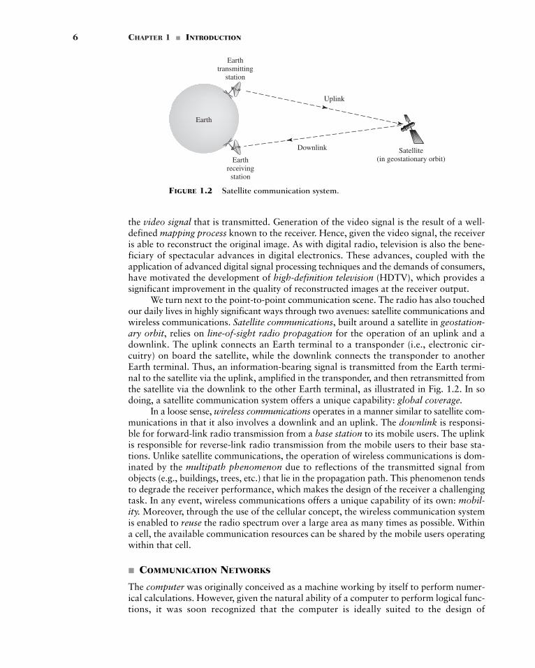
Satellite(in geostationary orbit)
FIGURE 1.2 Satellite communication system.
the video signal that is transmitted. Generation of the video signal is the result of a well-defined mapping process known to the receiver. Hence, given the video signal, the receiveris able to reconstruct the original image. As with digital radio, television is also the bene-ficiary of spectacular advances in digital electronics. These advances, coupled with theapplication of advanced digital signal processing techniques and the demands of consumers,have motivated the development of high-definition television (HDTV), which provides asignificant improvement in the quality of reconstructed images at the receiver output.
We turn next to the point-to-point communication scene. The radio has also touchedour daily lives in highly significant ways through two avenues: satellite communications andwireless communications. Satellite communications, built around a satellite in geostation-ary orbit, relies on line-of-sight radio propagation for the operation of an uplink and adownlink. The uplink connects an Earth terminal to a transponder (i.e., electronic cir-cuitry) on board the satellite, while the downlink connects the transponder to anotherEarth terminal. Thus, an information-bearing signal is transmitted from the Earth termi-nal to the satellite via the uplink, amplified in the transponder, and then retransmitted fromthe satellite via the downlink to the other Earth terminal, as illustrated in Fig. 1.2. In sodoing, a satellite communication system offers a unique capability: global coverage.
In a loose sense, wireless communications operates in a manner similar to satellite com-munications in that it also involves a downlink and an uplink. The downlink is responsi-ble for forward-link radio transmission from a base station to its mobile users. The uplinkis responsible for reverse-link radio transmission from the mobile users to their base sta-tions. Unlike satellite communications, the operation of wireless communications is dom-inated by the multipath phenomenon due to reflections of the transmitted signal fromobjects (e.g., buildings, trees, etc.) that lie in the propagation path. This phenomenon tendsto degrade the receiver performance, which makes the design of the receiver a challengingtask. In any event, wireless communications offers a unique capability of its own: mobil-ity. Moreover, through the use of the cellular concept, the wireless communication systemis enabled to reuse the radio spectrum over a large area as many times as possible. Withina cell, the available communication resources can be shared by the mobile users operatingwithin that cell.
� COMMUNICATION NETWORKS
The computer was originally conceived as a machine working by itself to perform numer-ical calculations. However, given the natural ability of a computer to perform logical func-tions, it was soon recognized that the computer is ideally suited to the design of
1.2 Applications 7
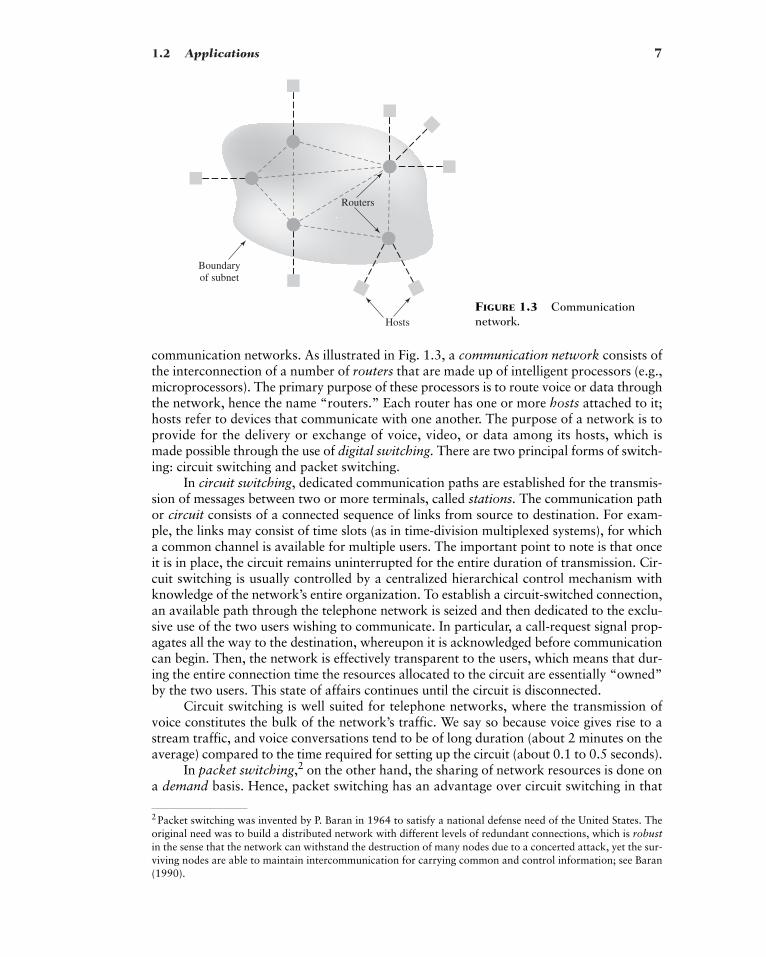
Hosts
Boundaryof subnet
Routers
FIGURE 1.3 Communicationnetwork.
communication networks. As illustrated in Fig. 1.3, a communication network consists ofthe interconnection of a number of routers that are made up of intelligent processors (e.g.,microprocessors). The primary purpose of these processors is to route voice or data throughthe network, hence the name “routers.” Each router has one or more hosts attached to it;hosts refer to devices that communicate with one another. The purpose of a network is toprovide for the delivery or exchange of voice, video, or data among its hosts, which ismade possible through the use of digital switching. There are two principal forms of switch-ing: circuit switching and packet switching.
In circuit switching, dedicated communication paths are established for the transmis-sion of messages between two or more terminals, called stations. The communication pathor circuit consists of a connected sequence of links from source to destination. For exam-ple, the links may consist of time slots (as in time-division multiplexed systems), for whicha common channel is available for multiple users. The important point to note is that onceit is in place, the circuit remains uninterrupted for the entire duration of transmission. Cir-cuit switching is usually controlled by a centralized hierarchical control mechanism withknowledge of the network’s entire organization. To establish a circuit-switched connection,an available path through the telephone network is seized and then dedicated to the exclu-sive use of the two users wishing to communicate. In particular, a call-request signal prop-agates all the way to the destination, whereupon it is acknowledged before communicationcan begin. Then, the network is effectively transparent to the users, which means that dur-ing the entire connection time the resources allocated to the circuit are essentially “owned”by the two users. This state of affairs continues until the circuit is disconnected.
Circuit switching is well suited for telephone networks, where the transmission ofvoice constitutes the bulk of the network’s traffic. We say so because voice gives rise to astream traffic, and voice conversations tend to be of long duration (about 2 minutes on theaverage) compared to the time required for setting up the circuit (about 0.1 to 0.5 seconds).
In packet switching,2 on the other hand, the sharing of network resources is done ona demand basis. Hence, packet switching has an advantage over circuit switching in that
2 Packet switching was invented by P. Baran in 1964 to satisfy a national defense need of the United States. Theoriginal need was to build a distributed network with different levels of redundant connections, which is robustin the sense that the network can withstand the destruction of many nodes due to a concerted attack, yet the sur-viving nodes are able to maintain intercommunication for carrying common and control information; see Baran(1990).
8 CHAPTER 1 � INTRODUCTION
3 The OSI reference model was developed by a subcommittee of the International Organization for Standardiza-tion (ISO) in 1977. For a discussion of the principles involved in arriving at the original seven layers of the OSImodel and a description of the layers themselves, see Tannenbaum (1996).
when a link has traffic to send, the link tends to be more fully utilized. Unlike voice sig-nals, data tend to occur in the form of bursts on an occasional basis.
The network principle of packet switching is store and forward. Specifically, in apacket-switched network, any message longer than a specified size is subdivided prior totransmission into segments not exceeding the specified size. The segments so formed arecalled packets. After transporting the packets across different parts of the network, theoriginal message is reassembled at the destination on a packet-by-packet basis. The networkmay thus be viewed as a pool of network resources (i.e., channel bandwidth, buffers, andswitching processors), with the resources being dynamically shared by a community ofcompeting hosts that wish to communicate. This dynamic sharing of network resources isin direct contrast to the circuit-switched network, where the resources are dedicated to apair of hosts for the entire period they are in communication.
� DATA NETWORKS
A communication network in which the hosts are all made up of computers and terminalsis commonly referred to as a data network. The design of such a network proceeds in anorderly way by looking at the network in terms of a layered architecture, which is regardedas a hierarchy of nested layers. A layer refers to a process or device inside a computer sys-tem that is designed to perform a specific function. Naturally, the designers of a layer willbe familiar with its internal details and operation. At the system level, however, a userviews the layer in question merely as a “black box,” which is described in terms of inputs,outputs, and the functional relation between the outputs and inputs. In the layered archi-tecture, each layer regards the next lower layer as one or more black boxes with somegiven functional specification to be used by the given higher layer. In this way, the highlycomplex communication problem in data networks is resolved as a manageable set of well-defined interlocking functions. It is this line of reasoning that has led to the developmentof the open systems interconnection (OSI) reference model.3 The term “open” refers to theability of any two systems to interconnect, provided they conform to the reference modeland its associated standards.
In the OSI reference model, the communications and related-connection functionsare organized as a series of layers with well-defined interfaces. Each layer is built on its pre-decessor. In particular, each layer performs a related subset of primitive functions, and itrelies on the next lower layer to perform additional primitive functions. Moreover, each layeroffers certain services to the next higher layer and shields that layer from the implementa-tion details of those services. Between each pair of layers there is an interface, which definesthe services offered by the lower layer to the upper layer.
As illustrated in Fig. 1.4, the OSI model is composed of seven layers. The figure alsoincludes a description of the functions of the individual layers of the model. Layer k on sys-tem A, say, communicates with a layer R on some other system B in accordance with a setof rules and conventions, which collectively constitute layer k protocol, where k � 1, 2,. . . , 7. (The term “protocol” has been borrowed from common usage that describes con-ventional social behavior between human beings.) The entities that comprise the corre-sponding layers on different systems are referred to as peer processes. In other words,communication between system A and system B is achieved by having the peer processes inthe two systems communicate via protocol. Physical connection between peer processes
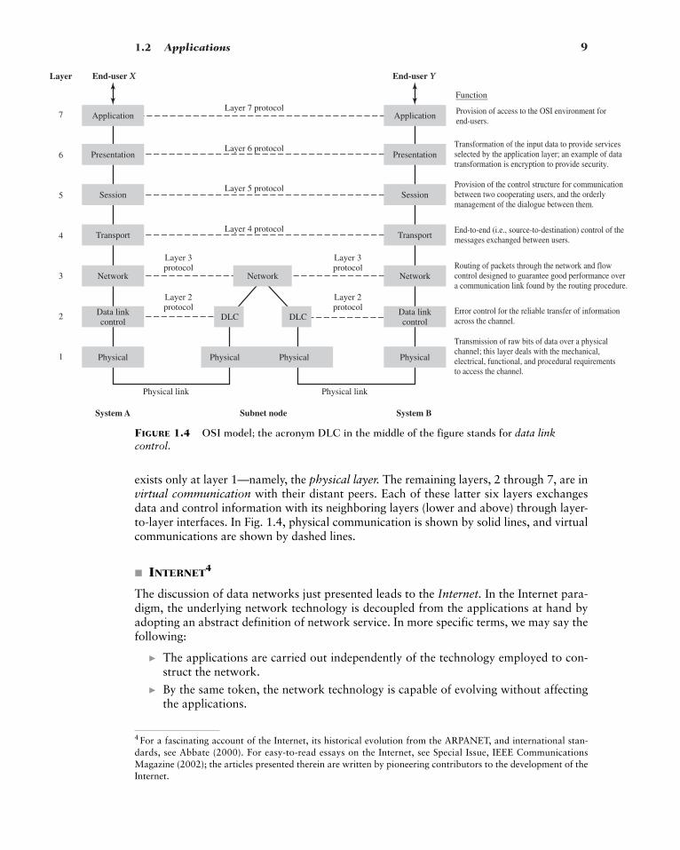
1.2 Applications 9
Provision of access to the OSI environment forend-users.
Transformation of the input data to provide servicesselected by the application layer; an example of datatransformation is encryption to provide security.
Provision of the control structure for communicationbetween two cooperating users, and the orderlymanagement of the dialogue between them.
End-to-end (i.e., source-to-destination) control of themessages exchanged between users.
Routing of packets through the network and flowcontrol designed to guarantee good performance overa communication link found by the routing procedure.
Error control for the reliable transfer of informationacross the channel.
Transmission of raw bits of data over a physicalchannel; this layer deals with the mechanical,electrical, functional, and procedural requirementsto access the channel.
7
6
5
4
3
2
1
System A Subnet node System B
Physical link
Layer 7 protocol
Layer 6 protocol
Layer 5 protocol
Layer 4 protocol
End-user XLayer End-user Y
Function
Layer 2protocol
Layer 3protocol
Physical Physical Physical Physical
Application Application
Presentation Presentation
Session Session
Transport Transport
Network Network Network
Physical link
Data linkcontrol
Data linkcontrol
DLC DLC
Layer 2protocol
Layer 3protocol
FIGURE 1.4 OSI model; the acronym DLC in the middle of the figure stands for data linkcontrol.
4 For a fascinating account of the Internet, its historical evolution from the ARPANET, and international stan-dards, see Abbate (2000). For easy-to-read essays on the Internet, see Special Issue, IEEE CommunicationsMagazine (2002); the articles presented therein are written by pioneering contributors to the development of theInternet.
exists only at layer 1—namely, the physical layer. The remaining layers, 2 through 7, are invirtual communication with their distant peers. Each of these latter six layers exchangesdata and control information with its neighboring layers (lower and above) through layer-to-layer interfaces. In Fig. 1.4, physical communication is shown by solid lines, and virtualcommunications are shown by dashed lines.
� INTERNET4
The discussion of data networks just presented leads to the Internet. In the Internet para-digm, the underlying network technology is decoupled from the applications at hand byadopting an abstract definition of network service. In more specific terms, we may say thefollowing:
� The applications are carried out independently of the technology employed to con-struct the network.
� By the same token, the network technology is capable of evolving without affectingthe applications.
10 CHAPTER 1 � INTRODUCTION
Router Router
Hosts Hosts
Subnet 2
Subnet 1 Subnet 3
... ...
Subnet 1 Subnet 1 Subnet 1
AP: Application protocolTCP: Transmission control protocol
UDP: User datagram protocolIP: Internet protocol
AP
IP
TCP/UDP
AP
IP
TCP/UDP
AP
IP
TCP/UDP
AP
IP
TCP/UDP
FIGURE 1.6 Illustrating the network architecture of the Internet.
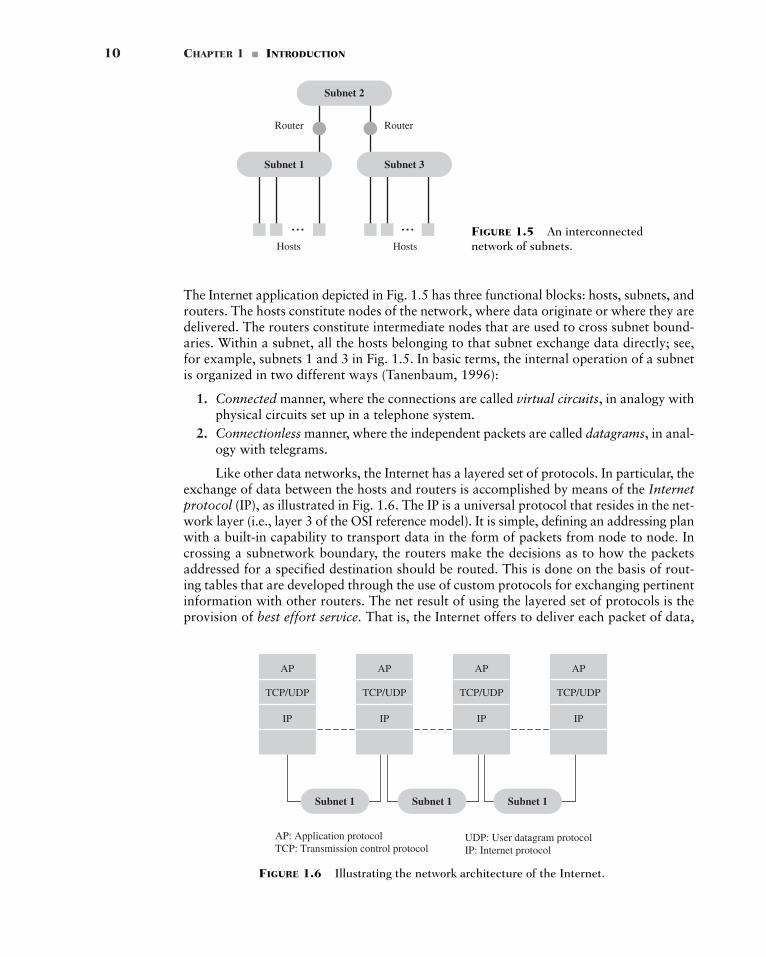
The Internet application depicted in Fig. 1.5 has three functional blocks: hosts, subnets, androuters. The hosts constitute nodes of the network, where data originate or where they aredelivered. The routers constitute intermediate nodes that are used to cross subnet bound-aries. Within a subnet, all the hosts belonging to that subnet exchange data directly; see,for example, subnets 1 and 3 in Fig. 1.5. In basic terms, the internal operation of a subnetis organized in two different ways (Tanenbaum, 1996):
1. Connected manner, where the connections are called virtual circuits, in analogy withphysical circuits set up in a telephone system.
2. Connectionless manner, where the independent packets are called datagrams, in anal-ogy with telegrams.
Like other data networks, the Internet has a layered set of protocols. In particular, theexchange of data between the hosts and routers is accomplished by means of the Internetprotocol (IP), as illustrated in Fig. 1.6. The IP is a universal protocol that resides in the net-work layer (i.e., layer 3 of the OSI reference model). It is simple, defining an addressing planwith a built-in capability to transport data in the form of packets from node to node. Incrossing a subnetwork boundary, the routers make the decisions as to how the packetsaddressed for a specified destination should be routed. This is done on the basis of rout-ing tables that are developed through the use of custom protocols for exchanging pertinentinformation with other routers. The net result of using the layered set of protocols is theprovision of best effort service. That is, the Internet offers to deliver each packet of data,
FIGURE 1.5 An interconnectednetwork of subnets.
1.2 Applications 11
but there are no guarantees on the transit time experienced in delivery or even whether thepackets will be delivered to the intended recipient.
The Internet has evolved into a worldwide system, placing computers at the heart ofa communication medium that is changing our daily lives in the home and workplace inprofound ways. We can send an e-mail message from a host in North America to anotherhost in Australia at the other end of the globe, with the message arriving at its destinationin a matter of seconds. This is all the more remarkable because the packets constituting themessage are quite likely to have taken entirely different paths as they are transported acrossthe network.
Another application that demonstrates the remarkable power of the Internet is ouruse of it to surf the Web. For example, we may use a search engine to identify the refer-ences pertaining to a particular subject of interest. A task that used to take hours and some-times days searching through books and journals in the library now occupies a matter ofseconds!
To fully utilize the computing power of the Internet from a host located at a remotesite, we need a wideband modem (i.e., modulator-demodulator) to provide a fast commu-nication link between that host and its subnet. When we say “fast,” we mean operatingspeeds on the order of megabits per second and higher. A device that satisfies this require-ment is the so-called digital subscriber line (DSL). What makes the DSL all the more remark-able is the fact that it can operate over a linear wideband channel with an arbitrary frequencyresponse. Such a channel is exemplified by an ordinary telephone channel built using twistedpairs for signal transmission. A twisted pair consists of two solid copper conductors, eachof which is encased in a polyvinyl chloride (PVC) sheath. Twisted pairs are usually madeup into cables, with each cable consisting of many twisted pairs in close proximity to eachother. From a signal-transmission viewpoint, the DSL satisfies the challenging requirementdescribed herein by following the well-known engineering principle of divide and conquer.Specifically, the given wideband channel is approximated by a set of narrowband channels,each of which can then be accommodated in a relatively straightforward manner.
One last comment is in order. Typically, access to the Internet is established via hostsin the form of computer terminals (i.e., servers). The access is expanded by using hand-helddevices that act as hosts, which communicate with subnets of the Internet via wireless links.Thus, by adding mobility through the use of wireless communications to the computingpower of the Internet to communicate, we have a new communication medium with enor-mous practical possibilities.
� INTEGRATION OF TELEPHONE AND INTERNET
One of the important challenges facing the telecommunications industry is the transmissionof Voice over Internet Protocol (VoIP), which would make it possible to integrate tele-phony services with the rapidly growing Internet-based applications. The challenge is allthe more profound because the IP is designed to accommodate the exchange of data betweenthe hosts and the routers, which makes it difficult to support quality of service for VoIP.Quality of service (QoS) is measured in terms of two parameters:
� Packet loss ratio, defined as the number of packets lost in transport across the net-work to the total number of packets pumped into the network.
� Connection delay, defined as the time taken for a packet of a particular host-to-hostconnection to transmit across the network.
Subjective tests performed on VoIP show that in order to provide voice-grade telephoneservice, the packet loss ratio must be held below 1 percent, and one-way connection delay
12 CHAPTER 1 � INTRODUCTION
5 The limits on QoS measures mentioned herein are taken from the overview article by James, Chen, and Garri-son (2004), which appears in a Special Issue of the IEEE Communications Magazine devoted to voice VoIP andquality of service.6 PBXs are discussed in McDonald (1990).
can accumulate up to 160 ms without significant degradation of quality. Well-designedand managed VoIP networks, satisfying these provisions, are being deployed. However,the issue of initial-echo control remains a challenge.5 Initial echo refers to the echo expe-rienced at the beginning of a call on the first word or couple of words out of a user’s mouth.The echo arises due to an impedance mismatch somewhere in the network, whereupon theincident signal is reflected back to the source.
Looking into the future, we may make the following remarks on internet telephony:
1. VoIP will replace private branch exchanges (PBXs) and other office switches; PBXsare remote switching units that have their own independent controls.6
2. VoIP is also currently having success with longer distance calls, but this is mainly dueto the excess capacity that is now available on long-haul networks. If the loading onthese long-haul networks increases, the delays will increase and a real-time service suchas VoIP will be degraded. Accordingly, if long-service providers keep adding capac-ity so that loading is always low and response time is fast, thereby ensuring qualityof service, then VoIP telephony may become mainstream and widespread.
� DATA STORAGE
When considering important applications of digital communication principles, it is nat-ural to think in terms of broadcasting and point-to-point communication systems. Never-theless, the very same principles are also applied to the digital storage of audio and videosignals, exemplified by compact disc (CD) and digital versatile disc (DVD) players. DVDsare refinements of CDs in that their storage capacity (in the order of tens of gigabytes) areorders of magnitude higher than that of CDs, and they can also deliver data at a muchhigher rate.
The digital domain is preferred over the analog domain for the storage of audio andvideo signals for the following compelling reasons:
(i) The quality of a digitized audio/video signal, measured in terms of frequency response,linearity, and noise, is determined by the digital-to-analog conversion (DAC) process,the parameterization of which is under the designer’s control.
(ii) Once the audio/video signal is digitized, we can make use of well-developed and pow-erful encoding techniques for data compression to reduce bandwidth, and error-con-trol coding to provide protection against the possibility of making errors in the courseof storage.
(iii) For most practical applications, the digital storage of audio and video signals does notdegrade with time.
(iv) Continued improvements in the fabrication of integrated circuits used to build CDsand DVDs ensure the ever-increasing cost-effectiveness of these digital storage devices.
With the help of the powerful encoding techniques built into their design, DVDs can holdhours of high-quality audio-visual contents, which, in turn, makes them ideally suited forinteractive multimedia applications.
1.3 Primary Resources and Operational Requirements 13
7 For a discussion of the decibel, see Appendix 1.
1.3 Primary Resources and Operational Requirements
The communication systems described in Section 1.2 cover many diverse fields. Neverthe-less, in their own individual ways, the systems are designed to provide for the efficient uti-lization of two primary communication resources:
� Transmitted power, which is defined as the average power of the transmitted signal.� Channel bandwidth, which is defined by the width of the passband of the channel.
Depending on which of these two resources is considered to be the limiting factor, we mayclassify communication channels as follows:
(i) Power-limited channels, where transmitted power is at a premium. Examples of suchchannels include the following:� Wireless channels, where it is desirable to keep the transmitted power low so as to
prolong battery life.� Satellite channels, where the available power on board the satellite transponder is
limited, which, in turn, necessitates keeping the transmitted power on the down-link at a low level.
� Deep-space links, where the available power on board a probe exploring outerspace is extremely limited, which again requires that the average power of infor-mation-bearing signals sent by the probe to an Earth station be maintained as lowas possible.
(ii) Band-limited channels, where channel bandwidth is at a premium. Examples of thissecond category of communication channels include the following:� Telephone channels, where, in a multi-user environment, the requirement is to
minimize the frequency band allocated to the transmission of each voice signalwhile making sure that the quality of service for each user is maintained.
� Television channels, where the available channel bandwidth is limited by regula-tory agencies and the quality of reception is assured by using a high enough trans-mitted power.
Another important point to keep in mind is the unavoidable presence of noise at thereceiver input of a communication system. In a generic sense, noise refers to unwanted sig-nals that tend to disturb the quality of the received signal in a communication system. Thesources of noise may be internal or external to the system. An example of internal noise isthe ubiquitous channel noise produced by thermal agitation of electrons in the front-endamplifier of the receiver. Examples of external noise include atmospheric noise and inter-ference due to transmitted signals pertaining to other users.
A quantitative way to account for the beneficial effect of the transmitted power in rela-tion to the degrading effect of noise (i.e., assess the quality of the received signal) is tothink in terms of the signal-to-noise ratio (SNR), which is a dimensionless parameter. In par-ticular, the SNR at the receiver input is formally defined as the ratio of the average powerof the received signal (i.e., channel output) to the average power of noise measured at thereceiver input. The customary practice is to express the SNR in decibels (dBs), which isdefined as 10 times the logarithm (to base 10) of the power ratio.7 For example, signal-to-noise ratios of 10, 100, and 1000 are 10, 20, and 30 dBs, respectively.
14 CHAPTER 1 � INTRODUCTION
8 One other theory—namely, Information Theory—is basic to the study of communication systems. We have notincluded this theory here because of its highly mathematical and therefore advanced nature, which makes it inap-propriate for an introductory book.
In light of this discussion, it is now apparent that as far as performance evaluation isconcerned, there are only two system-design parameters: signal-to-noise ratio and channelbandwidth. Stated in more concrete terms:
The design of a communication system boils down to a tradeoff between signal-to-noise ratio and channel bandwidth.
Thus, we may improve system performance by following one of two alternative designstrategies, depending on system constraints:
1. Signal-to-noise ratio is increased to accommodate a limitation imposed on channelbandwidth.
2. Channel bandwidth is increased to accommodate a limitation imposed on signal-to-noise ratio.
Of these two possible design approaches, we ordinarily find that strategy 1 is simpler toimplement than strategy 2, because increasing signal-to-noise ratio can be accomplished sim-ply by raising the transmitted power. On the other hand, in order to exploit increased chan-nel bandwidth, we need to increase the bandwidth of the transmitted signal, which, in turn,requires increasing the complexity of both the transmitter and receiver.
1.4 Underpinning Theories of Communication Systems
The study of communication systems is challenging not only in technical terms but also intheoretical terms. In this section, we highlight four theories, each of which is essential forunderstanding a specific aspect of communication systems.8
� MODULATION THEORY
Modulation is a signal-processing operation that is basic to the transmission of an infor-mation-bearing signal over a communication channel, whether in the context of digital oranalog communications. This operation is accomplished by changing some parameter ofa carrier wave in accordance with the information-bearing (message) signal. The carrier wavemay take one of two basic forms, depending on the application of interest:
� Sinusoidal carrier wave, whose amplitude, phase, or frequency is the parameter cho-sen for modification by the information-bearing signal.
� Periodic sequence of pulses, whose amplitude, width, or position is the parameterchosen for modification by the information-bearing signal.
Regardless of which particular approach is used to perform the modulation process,the issues in modulation theory that need to be addressed are:
� Time-domain description of the modulated signal.� Frequency-domain description of the modulated signal.� Detection of the original information-bearing signal and evaluation of the effect of
noise on the receiver.
1.4 Underpinning Theories of Communication Systems 15
� FOURIER ANALYSIS
The Fourier transform is a linear mathematical operation that transforms the time-domaindescription of a signal into a frequency-domain description without loss of information,which means that the original signal can be recovered exactly from the frequency-domaindescription. However, for the signal to be Fourier transformable, certain conditions haveto be satisfied. Fortunately, these conditions are satisfied by the kind of signals encounteredin the study of communication systems.
Fourier analysis provides the mathematical basis for evaluating the following issues:
� Frequency-domain description of a modulated signal, including its transmission band-width.
� Transmission of a signal through a linear system exemplified by a communicationchannel or (frequency-selective) filter.
� Correlation (i.e., similarity) between a pair of signals.
These evaluations take on even greater importance by virtue of an algorithm known as thefast Fourier transform, which provides an efficient method for computing the Fouriertransform.
� DETECTION THEORY
Given a received signal, which is perturbed by additive channel noise, one of the tasks thatthe receiver has to tackle is how to detect the original information-bearing signal in a reli-able manner. The signal-detection problem is complicated by two issues:
� The presence of noise.
� Factors such as the unknown phase-shift introduced into the carrier wave due totransmission of the sinusoidally modulated signal over the channel.
Dealing with these issues in analog communications is radically different from dealing withthem in digital communications. In analog communications, the usual approach focuses onoutput signal-to-noise ratio and related calculations. In digital communications, on theother hand, the signal-detection problem is viewed as one of hypothesis testing. For exam-ple, in the specific case of binary data transmission, given that binary symbol 1 is trans-mitted, what is the probability that the symbol is correctly detected, and how is thatprobability affected by a change in the received signal-to-noise ratio at the receiver input?
Thus, in dealing with detection theory, we address the following issues in analog com-munications:
� The figure of merit for assessing the noise performance of a specific modulationstrategy.
� The threshold phenomenon that arises when the transmitted signal-to-noise ratiodrops below a critical value.
� Performance comparison of one modulation strategy against another.
In digital communications, on the other hand, we look at:
� The average probability of symbol error at the receiver output.
� The issue of dealing with uncontrollable factors.
� Comparison of one digital modulation scheme against another.
16 CHAPTER 1 � INTRODUCTION
� PROBABILITY THEORY AND RANDOM PROCESSES
From the brief discussion just presented on the role of detection theory in the study of com-munication systems, it is apparent that we need to develop a good understanding of thefollowing:
� Probability theory for describing the behavior of randomly occurring events in math-ematical terms.
� Statistical characterization of random signals and noise.
Unlike a deterministic signal, a random signal is a signal about which there is uncertaintybefore it occurs. Because of the uncertainty, a random signal may be viewed as belongingto an ensemble, or a group, of signals, with each signal in the ensemble having a differentwaveform from that of the others in the ensemble. Moreover, each signal within the ensem-ble has a certain probability of occurrence. The ensemble of signals is referred to as a ran-dom process or stochastic process. Examples of a random process include:
� Electrical noise generated in the front-end amplifier of a radio or television receiver.� Speech signal produced by a male or female speaker.� Video signal transmitted by the antenna of a TV broadcasting station.
In dealing with probability theory, random signals, and noise, we address the followingissues:
� Basic concepts of probability theory and probabilistic models.� Statistical description of a random process in terms of ensemble as well as temporal
averages.� Mathematical analysis and processing of random signals.
1.5 Concluding Remarks
In this chapter, we have given a historical account and applications of communicationsand a brief survey of underlying theories of communication systems. In addition, we pre-sented the following points to support our view that the study of this discipline is bothhighly challenging and truly exciting:
(i) Communication systems encompass many and highly diverse applications: radio,television, wireless communications, satellite communications, deep-space commu-nications, telephony, data networks, Internet, and quite a few others.
(ii) Digital communication has established itself as the dominant form of communication.Much of the progress that we have witnessed in the advancement of digital commu-nication systems can be traced to certain enabling theories and technologies, as sum-marized here:� Abstract mathematical ideas that are highly relevant to a deep understanding of the
processing of information-bearing signals and their transmission over physicalmedia.
� Digital signal-processing algorithms for the efficient computation of spectra, cor-relation, and filtering of signals.
� Software development and novel architectures for designing microprocessors.� Spectacular advances in the physics of solid-state devices and the fabrication of very-
large-scale integrated (VLSI) chips.
1.5 Concluding Remarks 17
(iii) The study of communication systems is a dynamic discipline, continually evolvingby exploiting new technological innovations in other disciplines and responding to newsocietal needs.
(iv) Last but by no means least, communication systems touch our daily lives both athome and in the workplace, and our lives would be much poorer without the wideavailability of communication devices that we take for granted.
The remainder of the book, encompassing ten chapters, provides an introductorytreatment of both analog and digital kinds of communication systems. The book should pre-pare the reader for going on to deepen his or her knowledge of a discipline that is bestdescribed as almost limitless in scope. This is especially the case given the trend toward theunification of wireline and wireless networks to accommodate the integrated transmissionof voice, video, and data.
18
CHAPTER 2
FOURIER REPRESENTATION
OF SIGNALS AND SYSTEMS
In mathematical terms, a signal is ordinarily described as a function of time, which is howwe usually see the signal when its waveform is displayed on an oscilloscope. However, aspointed out in Chapter 1, from the perspective of a communication system it is importantthat we know the frequency content of the signal in question. The mathematical tool thatrelates the frequency-domain description of the signal to its time-domain description is theFourier transform. There are in fact several versions of the Fourier transform available. Inthis chapter, we confine the discussion primarily to two specific versions:
� The continuous Fourier transform, or the Fourier transform (FT) for short, whichworks with continuous functions in both the time and frequency domains.
� The discrete Fourier transform, or DFT for short, which works with discrete data inboth the time and frequency domains.
Much of the material presented in this chapter focuses on the Fourier transform, sincethe primary motivation of the chapter is to determine the frequency content of a continu-ous-time signal or to evaluate what happens to this frequency content when the signal ispassed through a linear time-invariant (LTI) system. In contrast, the discrete Fourier trans-form, discussed toward the end of the chapter, comes into its own when the requirement isto evaluate the frequency content of the signal on a digital computer or to evaluate whathappens to the signal when it is processed by a digital device as in digital communications.
The extensive material presented in this chapter teaches the following lessons:
� Lesson 1: The Fourier transform of a signal specifies the complex amplitudes of the com-ponents that constitute the frequency-domain description or spectral content of the signal.The inverse Fourier transform uniquely recovers the signal, given its frequency-domaindescription.
� Lesson 2: The Fourier transform is endowed with several important properties, which,individually and collectively, provide invaluable insight into the relationship between a sig-nal defined in the time domain and its frequency domain description.
� Lesson 3: A signal can only be strictly limited in the time domain or the frequency domain,but not both.
� Lesson 4: Bandwidth is an important parameter in describing the spectral content of a sig-nal and the frequency response of a linear time-invariant filter.
2.1 The Fourier Transform 19
1Joseph Fourier studied the flow of heat in the early 19th century. Understanding heat flow was a problem of bothpractical and scientific significance at that time and required solving a partial-differential equation called the heatequation. Fourier developed a technique for solving partial-differential equations that was based on the assump-tion that the solution was a weighted sum of harmonically related sinusoids with unknown coefficients, whichwe now term the Fourier series. Fourier’s initial work on heat conduction was submitted as a paper to the Acad-emy of Sciences of Paris in 1807 and rejected after review by Lagrange, Laplace, and Legendre. Fourier persistedin developing his ideas in spite of being criticized for a lack of rigor by his contemporaries. Eventually, in 1822,he published a book containing much of his work, Theorie analytique de la chaleur, which is now regarded asone of the classics of mathematics.
� Lesson 5: A widely used algorithm called the fast Fourier transform algorithm provides apowerful tool for computing the discrete Fourier transform; it is the mathematical tool fordigital computations involving Fourier transformation.
2.1 The Fourier Transform1
� DEFINITIONS
Let denote a nonperiodic deterministic signal, expressed as some function of time t.By definition, the Fourier transform of the signal is given by the integral
(2.1)
where and the variable denotes frequency; the exponential functionis referred to as the kernel of the formula defining the Fourier transform.
Given the Fourier transform the original signal is recovered exactly using the for-mula for the inverse Fourier transform:
(2.2)
where the exponential is the kernel of the formula defining the inverse Fouriertransform. The two kernels of Eqs. (2.1) and (2.2) are therefore the complex conjugate ofeach other.
Note also that in Eqs. (2.1) and (2.2) we have used a lowercase letter to denote thetime function and an uppercase letter to denote the corresponding frequency function. Thefunctions and are said to constitute a Fourier-transform pair. In Appendix 2, wederive the definitions of the Fourier transform and its inverse, starting from the Fourier seriesof a periodic waveform.
We refer to Eq. (2.1) as the analysis equation. Given the time-domain behavior of asystem, we are enabled to analyze the frequency-domain behavior of a system. The basicadvantage of transforming the time-domain behavior into the frequency domain is thatresolution into eternal sinusoids presents the behavior as the superposition of steady-stateeffects. For systems whose time-domain behavior is described by linear differential equa-tions, the separate steady-state solutions are usually simple to understand in theoretical aswell as experimental terms.
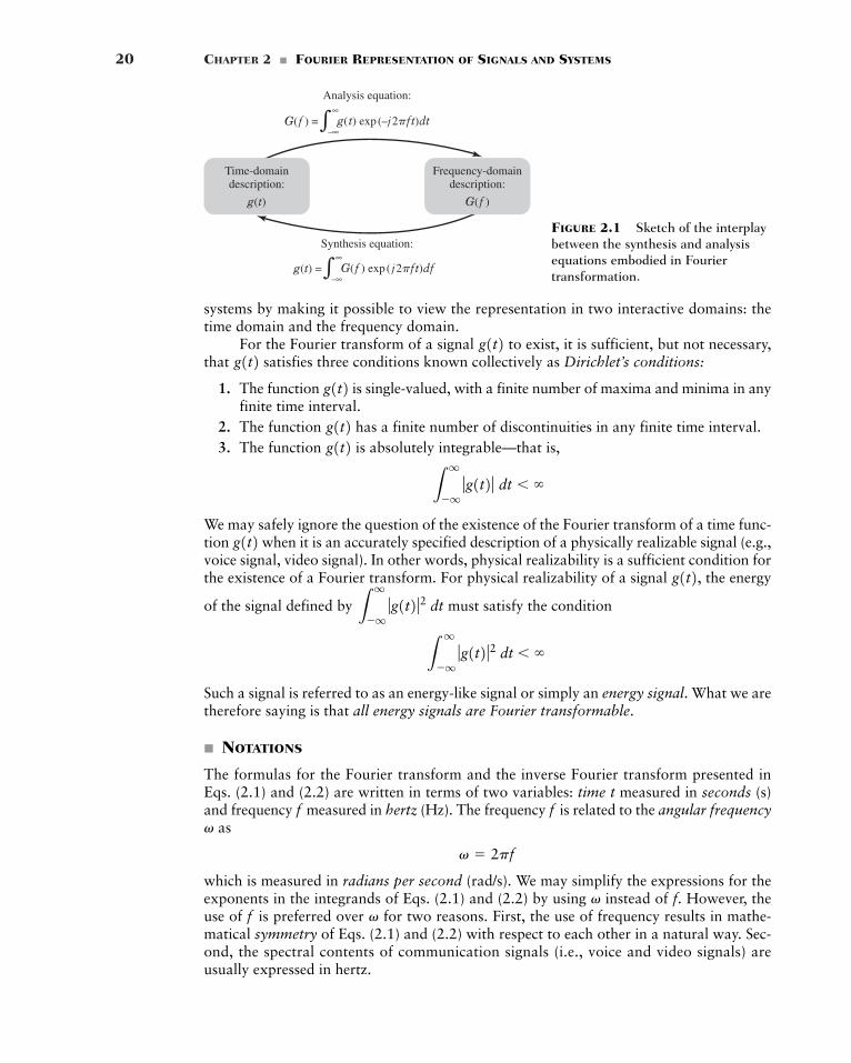
Conversely, we refer to Eq. (2.2) as the synthesis equation. Given the superpositionof steady-state effects in the frequency-domain, we can reconstruct the original time-domainbehavior of the system without any loss of information. The analysis and synthesis equa-tions, working side by side as depicted in Fig. 2.1, enrich the representation of signals and
G1f2g1t2
exp1j2pft2g1t2 � L
q
�qG1f2 exp1j2pft2 df
g1t2G1f2,exp1�j2pft2 fj � 2�1,
G1f 2 � Lq
�qg1t2 exp1�j2pft2 dt
g1t2g1t2
20 CHAPTER 2 � FOURIER REPRESENTATION OF SIGNALS AND SYSTEMS
Analysis equation:
Synthesis equation:
g(t) =
Time-domaindescription:
g(t)
Frequency-domaindescription:
G(f )
G(f ) exp ( j2�ft)df∞
–∞�
G(f ) = g(t) exp (–j2�ft)dt∞
–∞�
systems by making it possible to view the representation in two interactive domains: thetime domain and the frequency domain.
For the Fourier transform of a signal to exist, it is sufficient, but not necessary,that satisfies three conditions known collectively as Dirichlet’s conditions:
1. The function is single-valued, with a finite number of maxima and minima in anyfinite time interval.
2. The function has a finite number of discontinuities in any finite time interval.3. The function is absolutely integrable—that is,
We may safely ignore the question of the existence of the Fourier transform of a time func-tion when it is an accurately specified description of a physically realizable signal (e.g.,voice signal, video signal). In other words, physical realizability is a sufficient condition forthe existence of a Fourier transform. For physical realizability of a signal , the energy
of the signal defined by must satisfy the condition
Such a signal is referred to as an energy-like signal or simply an energy signal. What we aretherefore saying is that all energy signals are Fourier transformable.
� NOTATIONS
The formulas for the Fourier transform and the inverse Fourier transform presented inEqs. (2.1) and (2.2) are written in terms of two variables: time t measured in seconds (s)and frequency measured in hertz (Hz). The frequency is related to the angular frequency
as
which is measured in radians per second (rad/s). We may simplify the expressions for theexponents in the integrands of Eqs. (2.1) and (2.2) by using instead of However, theuse of is preferred over for two reasons. First, the use of frequency results in mathe-matical symmetry of Eqs. (2.1) and (2.2) with respect to each other in a natural way. Sec-ond, the spectral contents of communication signals (i.e., voice and video signals) areusually expressed in hertz.
vff.v
v � 2pf
v
ff
Lq
�qƒg1t2 ƒ2 dt � �
Lq
�qƒg1t2 ƒ2 dt
g1t2g1t2
Lq
�qƒg1t2 ƒ dt � �
g1t2g1t2g1t2
g1t2 g1t2
FIGURE 2.1 Sketch of the interplaybetween the synthesis and analysisequations embodied in Fouriertransformation.
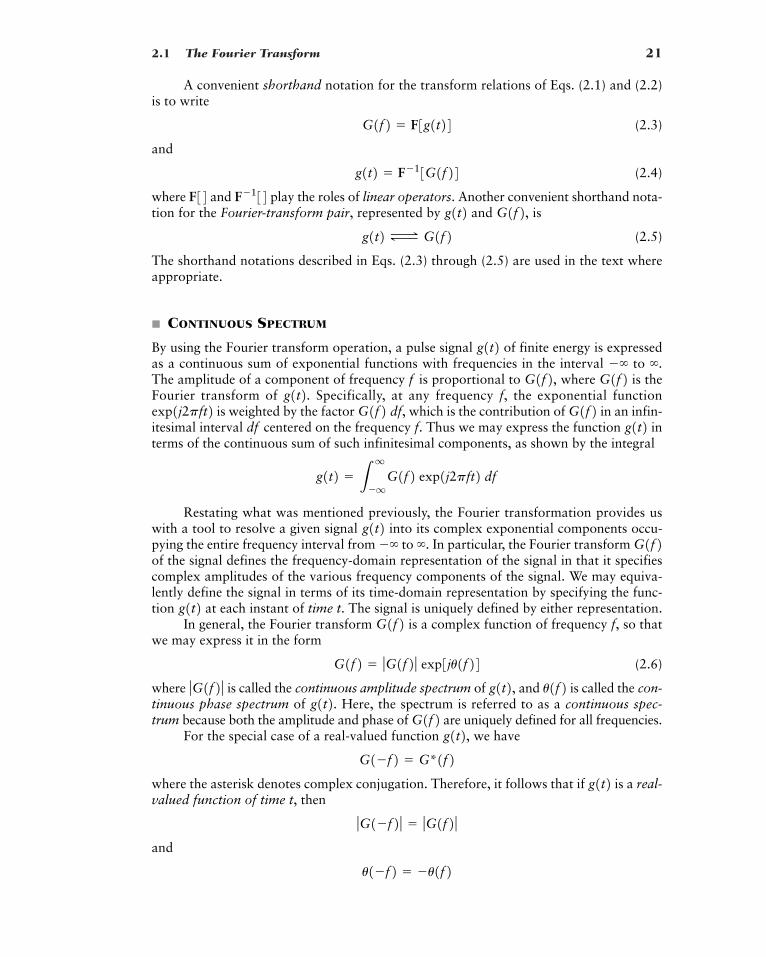
2.1 The Fourier Transform 21
A convenient shorthand notation for the transform relations of Eqs. (2.1) and (2.2)is to write
(2.3)
and
(2.4)
where and play the roles of linear operators. Another convenient shorthand nota-tion for the Fourier-transform pair, represented by and is
(2.5)
The shorthand notations described in Eqs. (2.3) through (2.5) are used in the text whereappropriate.
� CONTINUOUS SPECTRUM
By using the Fourier transform operation, a pulse signal of finite energy is expressedas a continuous sum of exponential functions with frequencies in the interval to The amplitude of a component of frequency is proportional to where is theFourier transform of Specifically, at any frequency the exponential function
is weighted by the factor which is the contribution of in an infin-itesimal interval centered on the frequency Thus we may express the function interms of the continuous sum of such infinitesimal components, as shown by the integral
Restating what was mentioned previously, the Fourier transformation provides uswith a tool to resolve a given signal into its complex exponential components occu-pying the entire frequency interval from to In particular, the Fourier transform of the signal defines the frequency-domain representation of the signal in that it specifiescomplex amplitudes of the various frequency components of the signal. We may equiva-lently define the signal in terms of its time-domain representation by specifying the func-tion at each instant of time t. The signal is uniquely defined by either representation.
In general, the Fourier transform is a complex function of frequency so thatwe may express it in the form
(2.6)
where is called the continuous amplitude spectrum of and is called the con-tinuous phase spectrum of Here, the spectrum is referred to as a continuous spec-trum because both the amplitude and phase of are uniquely defined for all frequencies.
For the special case of a real-valued function we have
where the asterisk denotes complex conjugation. Therefore, it follows that if is a real-valued function of time t, then
and
u1�f2 � �u1f2ƒG1�f2 ƒ � ƒG1f2 ƒ
g1t2G1�f2 � G*1f2
g1t2,G1f2g1t2. u1f2g1t2,ƒG1f2 ƒG1f2 � ƒG1f2 ƒ exp3ju1f24
f,G1f2g1t2
G1f2�.��g1t2
g1t2 � Lq
�qG1f2 exp1j2pft2 df
g1t2f.dfG1f2G1f2 df,exp1j2pft2 f,g1t2. G1f2G1f2,f
�.��g1t2
g1t2 Δ G1f2G1f2,g1t2F�134F34
g1t2 � F�13G1f24G1f2 � F3g1t24
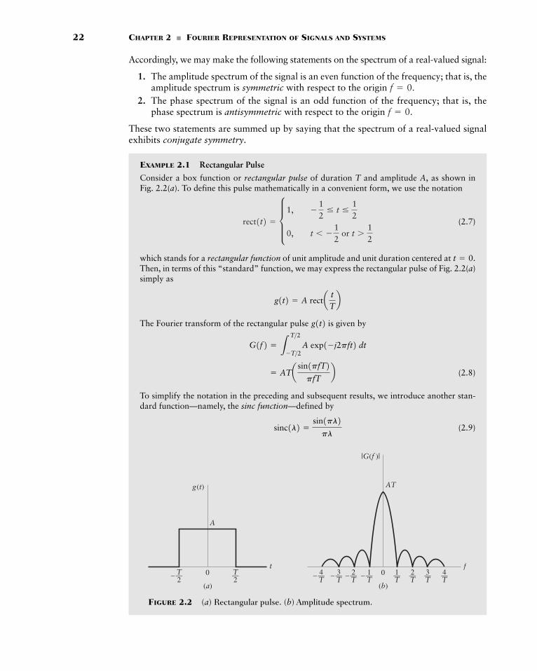
22 CHAPTER 2 � FOURIER REPRESENTATION OF SIGNALS AND SYSTEMS
Accordingly, we may make the following statements on the spectrum of a real-valued signal:
1. The amplitude spectrum of the signal is an even function of the frequency; that is, theamplitude spectrum is symmetric with respect to the origin
2. The phase spectrum of the signal is an odd function of the frequency; that is, thephase spectrum is antisymmetric with respect to the origin
These two statements are summed up by saying that the spectrum of a real-valued signalexhibits conjugate symmetry.
EXAMPLE 2.1 Rectangular Pulse
Consider a box function or rectangular pulse of duration T and amplitude A, as shown inFig. 2.2(a). To define this pulse mathematically in a convenient form, we use the notation
(2.7)
which stands for a rectangular function of unit amplitude and unit duration centered at Then, in terms of this “standard” function, we may express the rectangular pulse of Fig. 2.2(a)simply as
The Fourier transform of the rectangular pulse is given by
(2.8)
To simplify the notation in the preceding and subsequent results, we introduce another stan-dard function—namely, the sinc function—defined by
(2.9)sinc1l2 �sin1pl2pl
� ATa sin1pfT2pfT
bG1f2 � L
T>2�T>2 A exp1�j2pft2 dt
g1t2g1t2 � A recta t
Tb
t � 0.
rect1t2 � d 1, �12
� t �12
0, t � �12
or t �12
f � 0.
f � 0.
0 T
g(t)
(a)
A
2
t—T
2—– 0
|G(f )|
(b)
AT
f4T— 4
T—– 3
T— 3
T—– 2
T— 2
T—– 1
T— 1
T—–
FIGURE 2.2 (a) Rectangular pulse. (b) Amplitude spectrum.
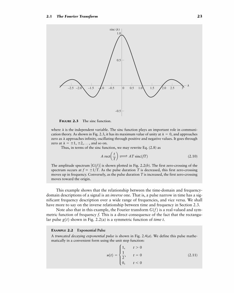
2.1 The Fourier Transform 23
0
sinc (�)
�–0.5 0.5 1.0 1.5 2.0 2.5 3–1.0–1.5–2.0–2.5
0.5
–0.5
1.0
FIGURE 2.3 The sinc function.
where is the independent variable. The sinc function plays an important role in communi-cation theory. As shown in Fig. 2.3, it has its maximum value of unity at and approacheszero as approaches infinity, oscillating through positive and negative values. It goes throughzero at and so on.
Thus, in terms of the sinc function, we may rewrite Eq. (2.8) as
(2.10)
The amplitude spectrum is shown plotted in Fig. 2.2(b). The first zero-crossing of thespectrum occurs at As the pulse duration T is decreased, this first zero-crossingmoves up in frequency. Conversely, as the pulse duration T is increased, the first zero-crossingmoves toward the origin.
This example shows that the relationship between the time-domain and frequency-domain descriptions of a signal is an inverse one. That is, a pulse narrow in time has a sig-nificant frequency description over a wide range of frequencies, and vice versa. We shallhave more to say on the inverse relationship between time and frequency in Section 2.3.
Note also that in this example, the Fourier transform is a real-valued and sym-metric function of frequency This is a direct consequence of the fact that the rectangu-lar pulse shown in Fig. 2.2(a) is a symmetric function of time t.
EXAMPLE 2.2 Exponential Pulse
A truncated decaying exponential pulse is shown in Fig. 2.4(a). We define this pulse mathe-matically in a convenient form using the unit step function:
(2.11)u1t2 � d 1, t � 012
, t � 0
0, t � 0
g1t2 f.G1f2
f � �1>T.ƒG1f2 ƒ
A recta tTb Δ AT sinc1fT2
l � �1, �2, Á ,l
l � 0,l
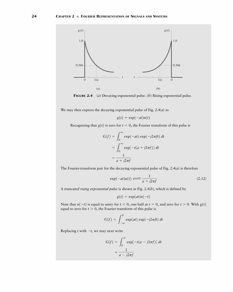
24 CHAPTER 2 � FOURIER REPRESENTATION OF SIGNALS AND SYSTEMS
(a)
0 1/a
0.366
1.0
0.366
1.0
g (t)
t t
(b)
01/a
g (t)
FIGURE 2.4 (a) Decaying exponential pulse. (b) Rising exponential pulse.
We may then express the decaying exponential pulse of Fig. 2.4(a) as
Recognizing that is zero for the Fourier transform of this pulse is
The Fourier-transform pair for the decaying exponential pulse of Fig. 2.4(a) is therefore
(2.12)
A truncated rising exponential pulse is shown in Fig. 2.4(b), which is defined by
Note that is equal to unity for one-half at and zero for With equal to zero for the Fourier transform of this pulse is
Replacing t with we may next write
�1
a � j2pf
G1f2 � Lq
0 exp3�t1a � j2pf24 dt
�t,
G1f2 � L0
�q exp1at2 exp1�j2pft2 dt
t � 0,g1t2t � 0.t � 0,t � 0,u1�t2
g1t2 � exp1at2u1�t2
exp1�at2u1t2 Δ1
a j2pf
�1
a j2pf
� Lq
0 exp3�t1a j2pf24 dt
G1f2 � Lq
0 exp1�at2 exp1�j2pft2 dt
t � 0,g1t2g1t2 � exp1�at2u1t2
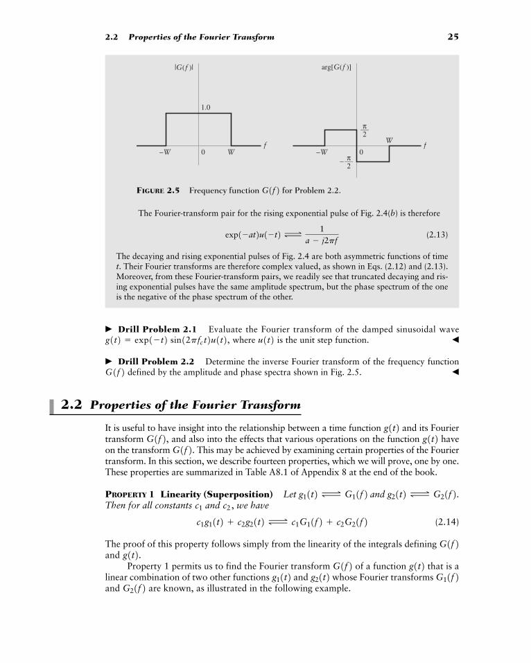
2.2 Properties of the Fourier Transform 25
0
1.0
|G(f )|
W–Wf
0
––2π
––2π
arg[G(f )]
W
–W–
f
The Fourier-transform pair for the rising exponential pulse of Fig. 2.4(b) is therefore
(2.13)
The decaying and rising exponential pulses of Fig. 2.4 are both asymmetric functions of timet. Their Fourier transforms are therefore complex valued, as shown in Eqs. (2.12) and (2.13).Moreover, from these Fourier-transform pairs, we readily see that truncated decaying and ris-ing exponential pulses have the same amplitude spectrum, but the phase spectrum of the oneis the negative of the phase spectrum of the other.
� Drill Problem 2.1 Evaluate the Fourier transform of the damped sinusoidal wavewhere is the unit step function. �
� Drill Problem 2.2 Determine the inverse Fourier transform of the frequency functiondefined by the amplitude and phase spectra shown in Fig. 2.5. �
2.2 Properties of the Fourier Transform
It is useful to have insight into the relationship between a time function and its Fouriertransform and also into the effects that various operations on the function haveon the transform This may be achieved by examining certain properties of the Fouriertransform. In this section, we describe fourteen properties, which we will prove, one by one.These properties are summarized in Table A8.1 of Appendix 8 at the end of the book.
PROPERTY 1 Linearity (Superposition) Let and Then for all constants and we have
(2.14)
The proof of this property follows simply from the linearity of the integrals defining and
Property 1 permits us to find the Fourier transform of a function that is alinear combination of two other functions and whose Fourier transforms and are known, as illustrated in the following example.G21f2 G11f2g21t2g11t2 g1t2G1f2g1t2. G1f2
c1g11t2 c2g21t2 Δ c1G11f2 c2G21f2c2,c1
g21t2 Δ G21f2.g11t2 Δ G11f2
G1f2. g1t2G1f2, g1t2
G1f2u1t2g1t2 � exp1�t2 sin12pfc t2u1t2,
exp1�at2u1�t2 Δ1
a � j2pf
FIGURE 2.5 Frequency function for Problem 2.2.G1f2
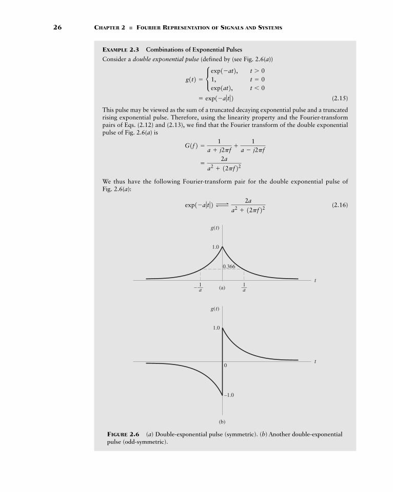
26 CHAPTER 2 � FOURIER REPRESENTATION OF SIGNALS AND SYSTEMS
0.366
t
g(t)
(a)
1.0
–1.0
0t
g(t)
(b)
1.0
– —1a —1a
FIGURE 2.6 (a) Double-exponential pulse (symmetric). (b) Another double-exponentialpulse (odd-symmetric).
EXAMPLE 2.3 Combinations of Exponential Pulses
Consider a double exponential pulse (defined by (see Fig. 2.6(a))
(2.15)
This pulse may be viewed as the sum of a truncated decaying exponential pulse and a truncatedrising exponential pulse. Therefore, using the linearity property and the Fourier-transformpairs of Eqs. (2.12) and (2.13), we find that the Fourier transform of the double exponentialpulse of Fig. 2.6(a) is
We thus have the following Fourier-transform pair for the double exponential pulse ofFig. 2.6(a):
(2.16)exp1�a ƒt ƒ2 Δ2a
a2 12pf22
�2a
a2 12pf22G1f2 �
1a j2pf
1
a � j2pf
� exp1�a ƒt ƒ2g1t2 � c exp1�at2, t � 0
1, t � 0exp1at2, t � 0
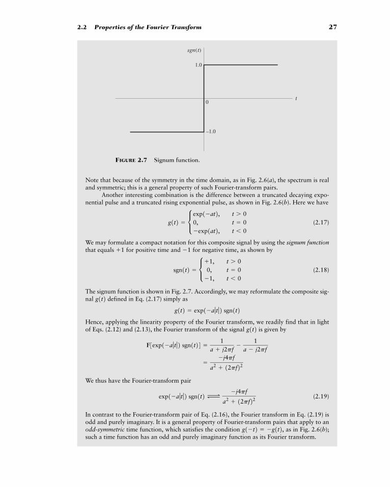
2.2 Properties of the Fourier Transform 27
1.0
–1.0
0t
sgn(t)
FIGURE 2.7 Signum function.
Note that because of the symmetry in the time domain, as in Fig. 2.6(a), the spectrum is realand symmetric; this is a general property of such Fourier-transform pairs.
Another interesting combination is the difference between a truncated decaying expo-nential pulse and a truncated rising exponential pulse, as shown in Fig. 2.6(b). Here we have
(2.17)
We may formulate a compact notation for this composite signal by using the signum functionthat equals for positive time and for negative time, as shown by
(2.18)
The signum function is shown in Fig. 2.7. Accordingly, we may reformulate the composite sig-nal defined in Eq. (2.17) simply as
Hence, applying the linearity property of the Fourier transform, we readily find that in lightof Eqs. (2.12) and (2.13), the Fourier transform of the signal is given by
We thus have the Fourier-transform pair
(2.19)
In contrast to the Fourier-transform pair of Eq. (2.16), the Fourier transform in Eq. (2.19) isodd and purely imaginary. It is a general property of Fourier-transform pairs that apply to anodd-symmetric time function, which satisfies the condition as in Fig. 2.6(b);such a time function has an odd and purely imaginary function as its Fourier transform.
g1�t2 � �g1t2,
exp1�a ƒt ƒ2 sgn1t2 Δ�j4pf
a2 12pf22
��j4pf
a2 12pf22F3exp1�a ƒt ƒ2 sgn1t24 �
1a j2pf
�1
a � j2pf
g1t2g1t2 � exp1�a ƒt ƒ2 sgn1t2
g1t2
sgn1t2 � c1, t � 00, t � 0
�1, t � 0
�11
g1t2 � c exp1�at2, t � 00, t � 0�exp1at2, t � 0
28 CHAPTER 2 � FOURIER REPRESENTATION OF SIGNALS AND SYSTEMS
PROPERTY 2 Dilation Let Then, the dilation property or similarityproperty states that
(2.20)
where the dilation factor—namely, a—is a real number.
To prove this property, we note that
Set There are two cases that can arise, depending on whether the dilation factor ais positive or negative. If we get
On the other hand, if the limits of integration are interchanged so that we have themultiplying factor or, equivalently, This completes the proof of Eq. (2.20).
Note that the dilation factors a and used in the time and frequency functions inEq. (2.20) are reciprocals. In particular, the function represents compressed intime by the factor a, whereas the function represents expanded in frequencyby the same factor a, assuming that Thus, the dilation rule states that the com-pression of a function in the time domain is equivalent to the expansion of its Fouriertransform in the frequency domain by the same factor, or vice versa.
For the special case when the dilation rule of Eq. (2.20) reduces to the reflec-tion property, which states that if then
(2.21)
Referring to Fig. 2.4, we see that the rising exponential pulse shown in part (b) of the fig-ure is the reflection of the decaying exponential pulse shown in part (a) with respect to thevertical axis. Hence, applying the reflection rule to Eq. (2.12) that pertains to the decay-ing exponential pulse, we readily see that the Fourier transform of the rising exponentialpulse is which is exactly what we have in Eq. (2.13).
PROPERTY 3 Conjugation Rule Let Then for a complex-valued timefunction we have
(2.22)
where the asterisk denotes the complex-conjugate operation.
To prove this property, we know from the inverse Fourier transform that
g1t2 � Lq
�qG1f2 exp1j2pft2 df
g*1t2 Δ G*1�f2g1t2, g1t2 Δ G1f2.
1>1a � j2pf2,
g1�t2 Δ G1�f2g1t2 Δ G1f2,a � �1,
G1f2 g1t2 0 � a � 1.G1f2G1f>a2 g1t2g1at21>a1> ƒa ƒ .�11>a2a � 0,
�1a
Ga fab
F3g1at24 �1a L
q
�qg1t2 exp c�j2pa f
abt d dt
a � 0,t � at.
F3g1at24 � Lq
�qg1at2 exp1�j2pft2 dt
g1at2 Δ1
ƒa ƒGa f
ab
g1t2 Δ G1f2.
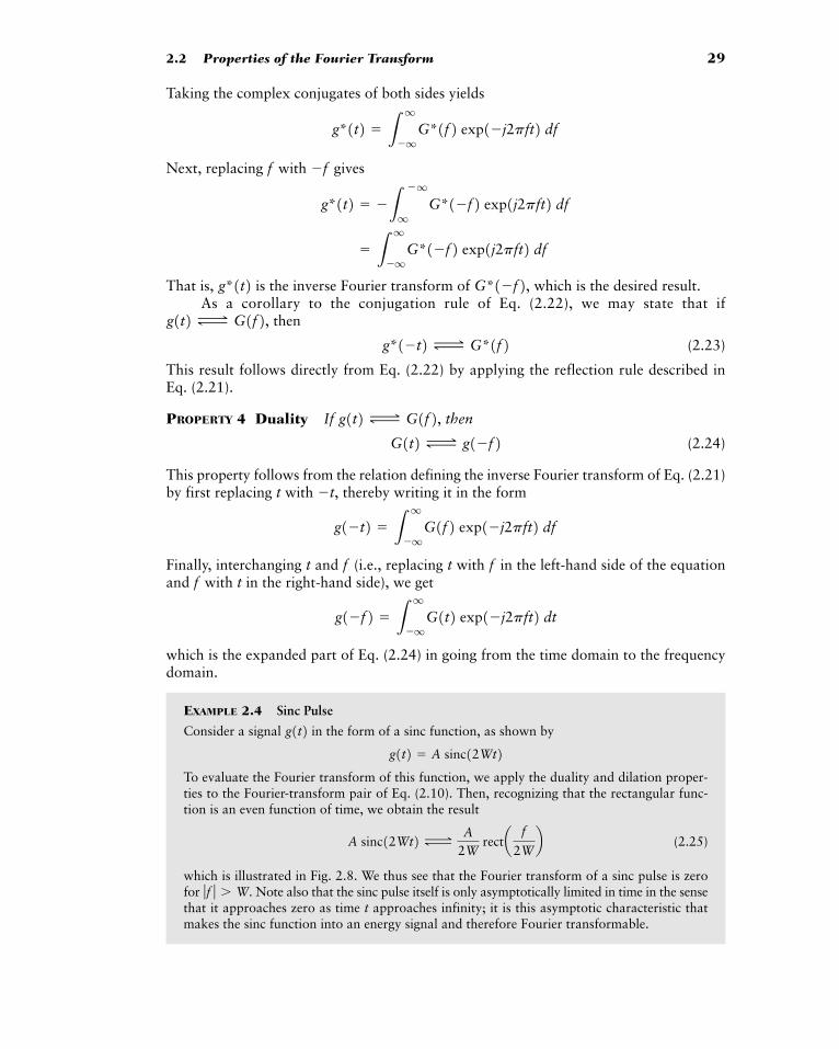
2.2 Properties of the Fourier Transform 29
Taking the complex conjugates of both sides yields
Next, replacing with gives
That is, is the inverse Fourier transform of which is the desired result.As a corollary to the conjugation rule of Eq. (2.22), we may state that if
then
(2.23)
This result follows directly from Eq. (2.22) by applying the reflection rule described inEq. (2.21).
PROPERTY 4 Duality If then
(2.24)
This property follows from the relation defining the inverse Fourier transform of Eq. (2.21)by first replacing t with thereby writing it in the form
Finally, interchanging t and (i.e., replacing t with in the left-hand side of the equationand with t in the right-hand side), we get
which is the expanded part of Eq. (2.24) in going from the time domain to the frequencydomain.
EXAMPLE 2.4 Sinc Pulse
Consider a signal in the form of a sinc function, as shown by
To evaluate the Fourier transform of this function, we apply the duality and dilation proper-ties to the Fourier-transform pair of Eq. (2.10). Then, recognizing that the rectangular func-tion is an even function of time, we obtain the result
(2.25)
which is illustrated in Fig. 2.8. We thus see that the Fourier transform of a sinc pulse is zerofor Note also that the sinc pulse itself is only asymptotically limited in time in the sensethat it approaches zero as time t approaches infinity; it is this asymptotic characteristic thatmakes the sinc function into an energy signal and therefore Fourier transformable.
ƒf ƒ � W.
A sinc12Wt2 ΔA
2W recta f
2Wb
g1t2 � A sinc12Wt2g1t2
g1�f2 � Lq
�qG1t2 exp1�j2pft2 dt
fff
g1�t2 � Lq
�qG1f2 exp1�j2pft2 df
�t,
G1t2 Δ g1�f2g1t2 Δ G1f2,
g*1�t2 Δ G*1f2g1t2 Δ G1f2,
G*1�f2,g*1t2� L
q
�qG*1�f2 exp1j2pft2 df
g*1t2 � �L�q
qG*1�f2 exp1j2pft2 df
�ff
g*1t2 � Lq
�qG*1f2 exp1�j2pft2 df
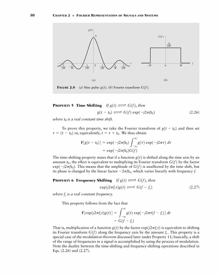
30 CHAPTER 2 � FOURIER REPRESENTATION OF SIGNALS AND SYSTEMS
PROPERTY 5 Time Shifting If then
(2.26)
where is a real constant time shift.
To prove this property, we take the Fourier transform of and then setor, equivalently, We thus obtain
The time-shifting property states that if a function is shifted along the time axis by anamount the effect is equivalent to multiplying its Fourier transform by the factor
This means that the amplitude of is unaffected by the time shift, butits phase is changed by the linear factor which varies linearly with frequency
PROPERTY 6 Frequency Shifting If then
(2.27)
where is a real constant frequency.
This property follows from the fact that
That is, multiplication of a function by the factor is equivalent to shiftingits Fourier transform along the frequency axis by the amount This property is aspecial case of the modulation theorem discussed later under Property 11; basically, a shiftof the range of frequencies in a signal is accomplished by using the process of modulation.Note the duality between the time-shifting and frequency-shifting operations described inEqs. (2.26) and (2.27).
fc .G1f2 exp1j2pfct2g1t2� G1f � fc2
F3exp1j2pfct2g1t24 � Lq
�qg1t2 exp3�j2pt1f � fc24 dt
fc
exp1j2pfct2g1t2 Δ G1f � fc2g1t2 Δ G1f2,
f.�2pft0,G1f2exp1�j2pft02. G1f2t0,
g1t2� exp1�j2pft02G1f2
F3g1t � t024 � exp1�j2pft02Lq
�qg1t2 exp1�j2pt2 dt
t � t t0.t � 1t � t02 g1t � t02t0
g1t � t02 Δ G1f2 exp1�j2pft02g1t2 Δ G1f2,
— 0
g(t)
G(f )
(a) (b)
A
t f3
2W—32W
—A2W
– 12W— 1
2W—–1
W— 1
W–W W0—–
FIGURE 2.8 (a) Sinc pulse (b) Fourier transform G1f2.g1t2.
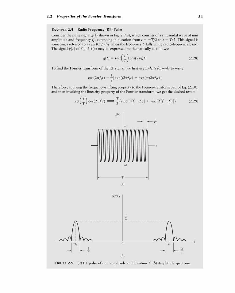
2.2 Properties of the Fourier Transform 31
|G(f )|
(b)
0f
–fc fc
g(t)
(a)
T
t
—T2
—2T
—1
+1
–1
fc
—2T
FIGURE 2.9 (a) RF pulse of unit amplitude and duration T. (b) Amplitude spectrum.
EXAMPLE 2.5 Radio Frequency (RF) Pulse
Consider the pulse signal shown in Fig. 2.9(a), which consists of a sinusoidal wave of unitamplitude and frequency extending in duration from to This signal issometimes referred to as an RF pulse when the frequency falls in the radio-frequency band.The signal of Fig. 2.9(a) may be expressed mathematically as follows:
(2.28)
To find the Fourier transform of the RF signal, we first use Euler’s formula to write
Therefore, applying the frequency-shifting property to the Fourier-transform pair of Eq. (2.10),and then invoking the linearity property of the Fourier transform, we get the desired result
(2.29)recta tTb cos12pfct2 Δ
T25sinc3T1f � fc24 sinc3T1f fc246
cos12pfct2 �123exp1j2pfct2 exp1�j2pfct24
g1t2 � recta tTb cos12pfct2
g1t2 fct � T>2.t � �T>2fc ,
g1t2
32 CHAPTER 2 � FOURIER REPRESENTATION OF SIGNALS AND SYSTEMS
In the special case of —that is, the frequency is large compared to the reciprocal ofthe pulse duration T—we may use the approximate result
(2.30)
Under the condition the amplitude spectrum of the RF pulse is shown in Fig. 2.9(b).This diagram, in relation to Fig. 2.2(b), clearly illustrates the frequency-shifting property of theFourier transform.
PROPERTY 7 Area Under If then
(2.31)
That is, the area under a function is equal to the value of its Fourier transform at
This result is obtained simply by putting in Eq. (2.1) defining the Fourier trans-form of the function
� Drill Problem 2.3 Suppose is real valued with a complex-valued Fourier transformExplain how the rule of Eq. (2.31) can be satisfied by such a signal. �
PROPERTY 8 Area Under If then
(2.32)
That is, the value of a function at is equal to the area under its Fourier trans-form
The result is obtained simply by putting in Eq. (2.2) defining the inverse Fouriertransform of
� Drill Problem 2.4 Continuing with Problem 2.3, explain how the rule of Eq. (2.32) canbe satisfied by the signal described therein. �
PROPERTY 9 Differentiation in the Time Domain Let and assumethat the first derivative of with respect to time t is Fourier transformable. Then
(2.33)
That is, differentiation of a time function has the effect of multiplying its Fourier trans-form by the purely imaginary factor
This result is obtained simply in two steps. In step 1, we take the first derivative ofboth sides of the integral in Eq. (2.2) defining the inverse Fourier transform of In step2, we interchange the operations of integration and differentiation.
G1f2.j2pf.G1f2 g1t2
ddt
g1t2 Δ j2pfG1f2g1t2 g1t2 Δ G1f2
g1t2G1f2. t � 0
G1f2. t � 0g1t2g102 � L
q
�qG1f2 df
g1t2 Δ G1f2,G1f2
G1f2. g1t2g1t2. f � 0
f � 0.G1f2g1t2
Lq
�qg1t2 dt � G102
g1t2 Δ G1f2,g1t2
fcT W 1,
G1f2 � e T2
sinc3T1f � fc24, f � 0
0, f � 0T2
sinc3T1f fc24, f � 0
fcfcT W 1
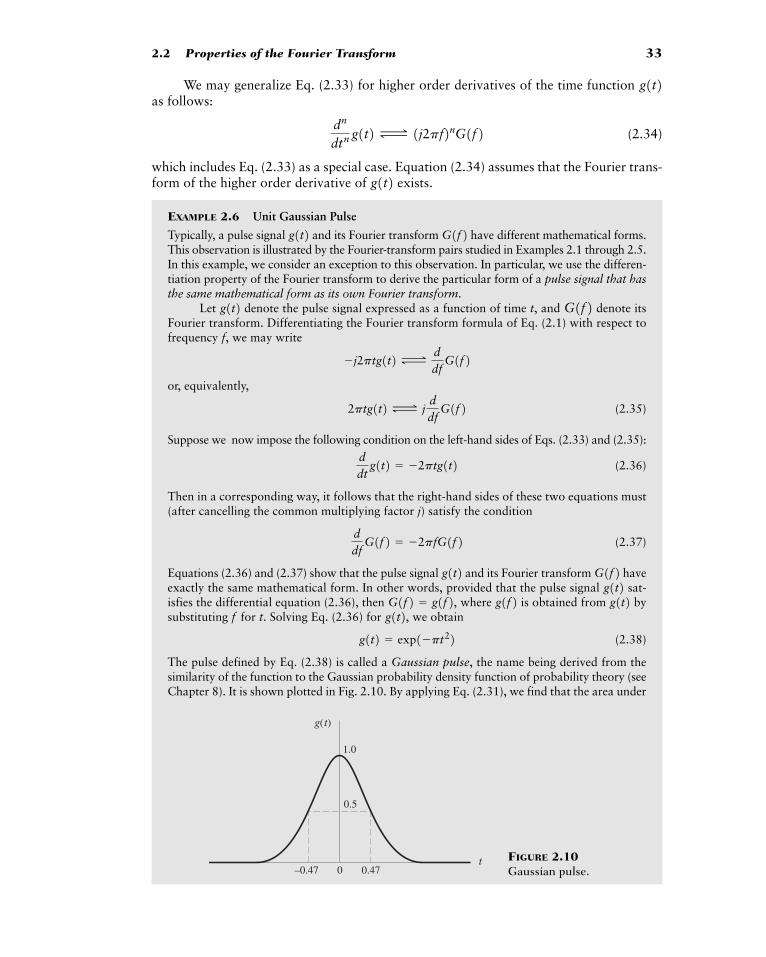
2.2 Properties of the Fourier Transform 33
We may generalize Eq. (2.33) for higher order derivatives of the time function as follows:
(2.34)
which includes Eq. (2.33) as a special case. Equation (2.34) assumes that the Fourier trans-form of the higher order derivative of exists.
EXAMPLE 2.6 Unit Gaussian Pulse
Typically, a pulse signal and its Fourier transform have different mathematical forms.This observation is illustrated by the Fourier-transform pairs studied in Examples 2.1 through 2.5.In this example, we consider an exception to this observation. In particular, we use the differen-tiation property of the Fourier transform to derive the particular form of a pulse signal that hasthe same mathematical form as its own Fourier transform.
Let denote the pulse signal expressed as a function of time t, and denote itsFourier transform. Differentiating the Fourier transform formula of Eq. (2.1) with respect tofrequency we may write
or, equivalently,
(2.35)
Suppose we now impose the following condition on the left-hand sides of Eqs. (2.33) and (2.35):
(2.36)
Then in a corresponding way, it follows that the right-hand sides of these two equations must(after cancelling the common multiplying factor j) satisfy the condition
(2.37)
Equations (2.36) and (2.37) show that the pulse signal and its Fourier transform haveexactly the same mathematical form. In other words, provided that the pulse signal sat-isfies the differential equation (2.36), then where is obtained from bysubstituting for t. Solving Eq. (2.36) for we obtain
(2.38)
The pulse defined by Eq. (2.38) is called a Gaussian pulse, the name being derived from thesimilarity of the function to the Gaussian probability density function of probability theory (seeChapter 8). It is shown plotted in Fig. 2.10. By applying Eq. (2.31), we find that the area under
g1t2 � exp1�pt22g1t2,f
g1t2g1f2G1f2 � g1f2, g1t2G1f2g1t2ddf
G1f2 � �2pfG1f2
ddt
g1t2 � �2ptg1t2
2ptg1t2 Δ jddf
G1f2
�j2ptg1t2 Δddf
G1f2f,
G1f2g1t2
G1f2g1t2
g1t2
dn
dtn g1t2 Δ 1j2pf2nG1f2g1t2
1.0
0–0.47 0.47
0.5
t
g(t)
FIGURE 2.10Gaussian pulse.
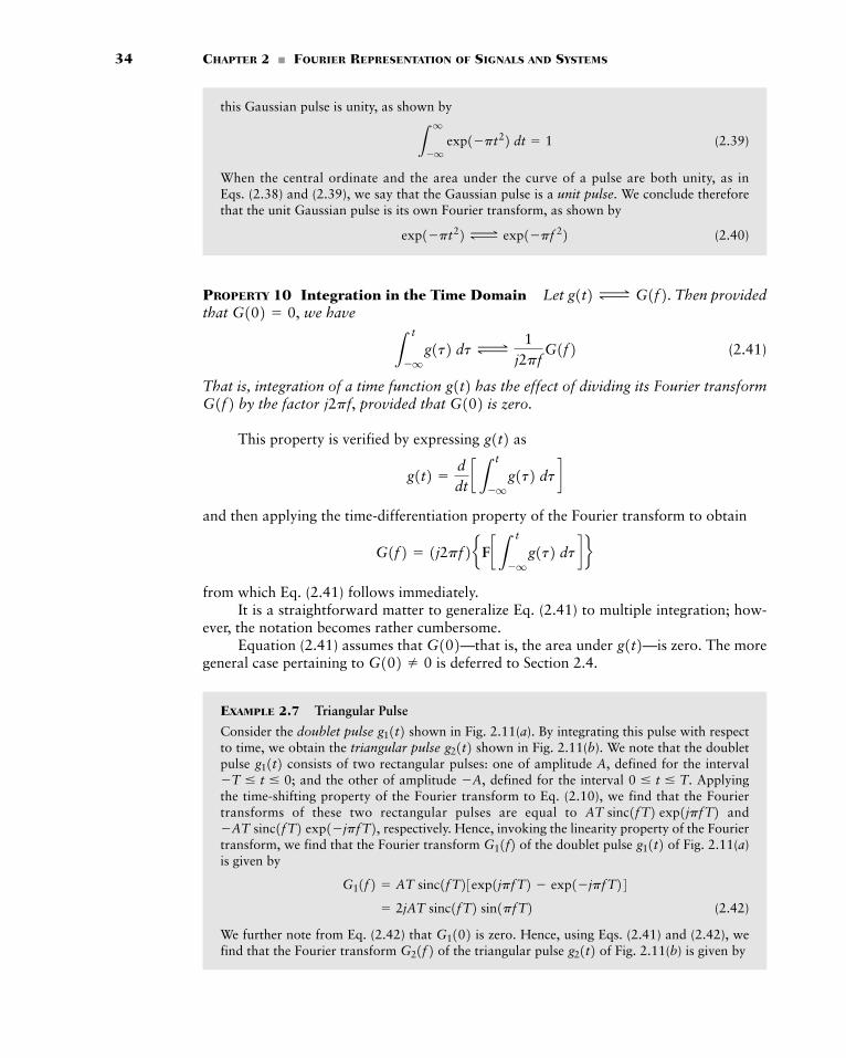
34 CHAPTER 2 � FOURIER REPRESENTATION OF SIGNALS AND SYSTEMS
this Gaussian pulse is unity, as shown by
(2.39)
When the central ordinate and the area under the curve of a pulse are both unity, as inEqs. (2.38) and (2.39), we say that the Gaussian pulse is a unit pulse. We conclude thereforethat the unit Gaussian pulse is its own Fourier transform, as shown by
(2.40)
PROPERTY 10 Integration in the Time Domain Let Then providedthat we have
(2.41)
That is, integration of a time function has the effect of dividing its Fourier transformby the factor provided that is zero.
This property is verified by expressing as
and then applying the time-differentiation property of the Fourier transform to obtain
from which Eq. (2.41) follows immediately.It is a straightforward matter to generalize Eq. (2.41) to multiple integration; how-
ever, the notation becomes rather cumbersome.Equation (2.41) assumes that —that is, the area under —is zero. The more
general case pertaining to is deferred to Section 2.4.
EXAMPLE 2.7 Triangular Pulse
Consider the doublet pulse shown in Fig. 2.11(a). By integrating this pulse with respectto time, we obtain the triangular pulse shown in Fig. 2.11(b). We note that the doubletpulse consists of two rectangular pulses: one of amplitude A, defined for the interval
and the other of amplitude defined for the interval Applyingthe time-shifting property of the Fourier transform to Eq. (2.10), we find that the Fouriertransforms of these two rectangular pulses are equal to and
respectively. Hence, invoking the linearity property of the Fouriertransform, we find that the Fourier transform of the doublet pulse of Fig. 2.11(a)is given by
(2.42)
We further note from Eq. (2.42) that is zero. Hence, using Eqs. (2.41) and (2.42), wefind that the Fourier transform of the triangular pulse of Fig. 2.11(b) is given byg21t2G21f2G1102
� 2jAT sinc1fT2 sin1pfT2G11f2 � AT sinc1fT23exp1jpfT2 � exp1�jpfT24
g11t2G11f2�AT sinc1fT2 exp1�jpfT2, AT sinc1fT2 exp1jpfT20 � t � T.�A,�T � t � 0;
g11t2 g21t2g11t2
G102 0g1t2G102
G1f2 � 1j2pf2eF cLt
�qg1t2 dt d f
g1t2 �ddtcL
t
�qg1t2 dt d
g1t2G102j2pf,G1f2 g1t2
Lt
�qg1t2 dt Δ
1j2pf
G1f2G102 � 0,
g1t2 Δ G1f2.
exp1�pt22 Δ exp1�pf 22
Lq
�q exp1�pt22 dt � 1
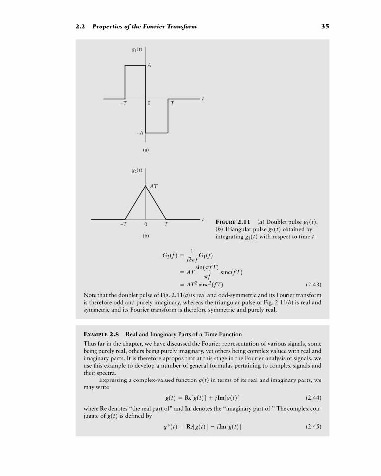
2.2 Properties of the Fourier Transform 35
0–T
–A
A
Tt
g1(t)
(a)
0–T
AT
Tt
g2(t)
(b)
FIGURE 2.11 (a) Doublet pulse (b) Triangular pulse obtained byintegrating with respect to time t.g11t2 g21t2 g11t2.
(2.43)
Note that the doublet pulse of Fig. 2.11(a) is real and odd-symmetric and its Fourier transformis therefore odd and purely imaginary, whereas the triangular pulse of Fig. 2.11(b) is real andsymmetric and its Fourier transform is therefore symmetric and purely real.
EXAMPLE 2.8 Real and Imaginary Parts of a Time Function
Thus far in the chapter, we have discussed the Fourier representation of various signals, somebeing purely real, others being purely imaginary, yet others being complex valued with real andimaginary parts. It is therefore apropos that at this stage in the Fourier analysis of signals, weuse this example to develop a number of general formulas pertaining to complex signals andtheir spectra.
Expressing a complex-valued function in terms of its real and imaginary parts, wemay write
(2.44)
where Re denotes “the real part of” and Im denotes the “imaginary part of.” The complex con-jugate of is defined by
(2.45)g*1t2 � Re3g1t24 � j Im3g1t24g1t2
g1t2 � Re3g1t24 j Im3g1t24g1t2
� AT2 sinc21fT2� AT
sin1pfT2pf
sinc1fT2G21f2 �
1j2pf
G11f2
36 CHAPTER 2 � FOURIER REPRESENTATION OF SIGNALS AND SYSTEMS
Adding Eqs. (2.44) and (2.45) gives
(2.46)
and subtracting them yields
(2.47)
Therefore, applying the conjugation rule of Eq. (2.22), we obtain the following two Fourier-transform pairs:
(2.48)
From the second line of Eq. (2.48), it is apparent that in the case of a real-valued time func-tion we have that is, the Fourier transform exhibits conjugatesymmetry, confirming a result that we stated previously in Section 2.2.
PROPERTY 11 Modulation Theorem Let and Then
(2.49)
To prove this property, we first denote the Fourier transform of the product byso that we may write
where
For we next substitute the inverse Fourier transform
in the integral defining to obtain
Define Then, eliminating the variable and interchanging the order of inte-gration, we obtain (after rearranging terms)
assuming that is fixed. The inner integral (inside the square brackets) is recognized sim-ply as we may therefore writeG11l2; f
G121f2 � Lq
�qG21f � l2c L
q
�qg11t2 exp1�j2plt2 dt d dl
f�l � f � f�.
G121f2 � Lq
�qLq
�qg11t2G21f�2 exp3�j2p1f � f�2t4 df�dt
G121f2g21t2 � L
q
�qG21f�2 exp1j2pf�t2 df�
g21t2,G121f2 � L
q
�qg11t2g21t2 exp1�j2pft2 dt
g11t2g21t2 Δ G121f2G121f2, g11t2g21t2
g11t2g21t2 Δ Lq
�qG11l2G21f � l2 dl
g21t2 Δ G21f2.g11t2 Δ G11f2
G1f2G1f2 � G*1�f2;g1t2,
Re3g1t24 Δ123G1f2 G*1�f24
Im3g1t2 Δ123G1f2 � G*1�f24 t
Im3g1t24 �123g1t2 � g*1t24
Re3g1t24 �123g1t2 g*1t24
2.2 Properties of the Fourier Transform 37
which is the desired result. This integral is known as the convolution integral expressed inthe frequency domain, and the function is referred to as the convolution ofand We conclude that the multiplication of two signals in the time domain is trans-formed into the convolution of their individual Fourier transforms in the frequency domain.This property is also known as the modulation theorem. We have more to say on the prac-tical implications of this property in subsequent chapters.
In a discussion of convolution, the following shorthand notation is frequently used:
Accordingly, we may reformulate Eq. (2.49) in the following symbolic form:
(2.50)
where the symbol denotes convolution. Note that convolution is commutative; that is,
which follows directly from Eq. (2.50).
PROPERTY 12 Convolution Theorem Let and Then
(2.51)
Equation (2.51) follows directly by combining Property 4 (duality) and Property 11(modulation). We may thus state that the convolution of two signals in the time domain istransformed into the multiplication of their individual Fourier transforms in the frequencydomain. This property is known as the convolution theorem. Its use permits us to exchangea convolution operation in the time domain for a multiplication of two Fourier transforms,an operation that is ordinarily easier to manipulate. We have more to say on convolutionlater in the chapter when the issue of filtering is discussed.
Using the shorthand notation for convolution, we may rewrite Eq. (2.51) in the sim-ple form
(2.52)
Note that Properties 11 and 12, described by Eqs. (2.49) and (2.51), respectively, are thedual of each other.
� Drill Problem 2.5 Develop the detailed steps that show that the modulation and con-volution theorems are indeed the dual of each other. �
PROPERTY 13 Correlation Theorem Let and Then, assuming that and are complex valued,
(2.53)
where is the complex conjugate of and is the time variable involved indefining the inverse Fourier transform of the product G11f2G2
…1f2.tG21f2,G2…1f2
Lq
�qg11t2g2
…1t � t2 dt Δ G11f2G2…1f2
g21t2g11t2 g21t2 Δ G21f2.g11t2 Δ G11f2
g11t2 � g21t2 Δ G11f2G21f2
Lq
�qg11t2g21t � t2 dt Δ G11f2G21f2
g21t2 Δ G21f2.g11t2 Δ G11f2
G11f2 � G21f2 � G21f2 � G11f2�
g11t2g21t2 Δ G11f2 � G21f2G121f2 � G11f2 � G21f2
G21f2. G11f2G121f2
G121f2 � Lq
�qG11l2G21f � l2 dl
38 CHAPTER 2 � FOURIER REPRESENTATION OF SIGNALS AND SYSTEMS
To prove Eq. (2.53), we begin by reformulating the convolution integral with the roles ofthe time variables t and interchanged, in which case we may simply rewrite Eq. (2.51) as
(2.54)
As already pointed out in the statement of Property 13, the inverse Fourier transform ofthe product term has as its time variable; that is, is its kernel. Withthe formula of Eq. (2.54) at hand, Eq. (2.53) follows directly by combining reflection rule(special case of the dilation property) and conjugation rule.
The integral on the left-hand side of Eq. (2.53) defines a measure of the similarity thatmay exist between a pair of complex-valued signals. This measure is called correlation, onwhich we have more to say later in the chapter.
� Drill Problem 2.6 Develop the detailed steps involved in deriving Eq. (2.53), startingfrom Eq. (2.51). �
� Drill Problem 2.7 Prove the following properties of the convolution process:
(a) The commutative property:
(b) The associative property:
(c) The distributive property:�
PROPERTY 14 Rayleigh’s Energy Theorem Let Then
(2.55)
To prove Eq. (2.55), we set in Eq. (2.53), in which case the correla-tion theorem reduces to
In expanded form, we may write
(2.56)
Finally, putting in Eq. (2.56) and recognizing that we get thedesired result.
Equation (2.55), known as Rayleigh’s energy theorem, states that the total energy ofa Fourier-transformable signal equals the total area under the curve of squared amplitudespectrum of this signal. Determination of the energy is often simplified by invoking theRayleigh energy theorem, as illustrated in the following example.
EXAMPLE 2.9 Sinc Pulse (continued)
Consider again the sinc pulse The energy of this pulse equals
E � A2
Lq
�qsinc212Wt2 dt
A sinc 12Wt2.
g1t2g*1t2 � ƒg1t2 ƒ2,t � 0
Lq
�qg1t2g*1t � t2 dt � L
q
�qƒG1f2 ƒ2 exp1j2pft2 df
Lq
�qg1t2g*1t � t2 dt Δ G1f2G*1f2 � ƒG1f2 ƒ2
g11t2 � g21t2 � g1t2L
q
�qƒg1t2 ƒ2 dt � L
q
�qƒG1f2 ƒ2 df
g1t2 Δ G1f2.
g11t2 � 3g21t2 g31t24 � g11t2 � g21t2 g11t2 � g31t2g11t2 � 3g21t2 � g31t24 � 3g11t2 � g21t24 � g31t2g11t2 � g21t2 � g21t2 � g11t2
exp1j2pft2tG11f2G21f2L
q
�qg11t2g21t � t2 dt Δ G11f2G21f2
t
2.3 The Inverse Relationship Between Time and Frequency 39
The integral in the right-hand side of this equation is rather difficult to evaluate. However, wenote from Example 2.4 that the Fourier transform of the sinc pulse is equal to
hence, applying Rayleigh’s energy theorem to the problem at hand, wereadily obtain the desired result:
(2.57)
This example clearly illustrates the usefulness of Rayleigh’s energy theorem.
� Drill Problem 2.8 Considering the pulse function show that
�
2.3 The Inverse Relationship Between Time and Frequency
The properties of the Fourier transform discussed in Section 2.2 show that the time-domainand frequency-domain descriptions of a signal are inversely related to each other. In par-ticular, we may make two important statements:
1. If the time-domain description of a signal is changed, the frequency-domain descrip-tion of the signal is changed in an inverse manner, and vice versa. This inverse rela-tionship prevents arbitrary specifications of a signal in both domains. In other words,we may specify an arbitrary function of time or an arbitrary spectrum, but we can-not specify both of them together.
2. If a signal is strictly limited in frequency, the time-domain description of the sig-nal will trail on indefinitely, even though its amplitude may assume a progres-sively smaller value. We say a signal is strictly limited in frequency or strictly bandlimited if its Fourier transform is exactly zero outside a finite band of frequen-cies. The sinc pulse is an example of a strictly band-limited signal, as illustratedin Fig. 2.8. This figure also shows that the sinc pulse is only asymptotically lim-ited in time. In an inverse manner, if a signal is strictly limited in time (i.e., the sig-nal is exactly zero outside a finite time interval), then the spectrum of the signalis infinite in extent, even though the amplitude spectrum may assume a progres-sively smaller value. This behavior is exemplified by both the rectangular pulse(described in Fig. 2.2) and the triangular pulse (described in Fig. 2.11(b)). Accord-ingly, we may state that a signal cannot be strictly limited in both time andfrequency.
� BANDWIDTH
The bandwidth of a signal provides a measure of the extent of the significant spectral con-tent of the signal for positive frequencies. When the signal is strictly band limited, the band-width is well defined. For example, the sinc pulse described in Fig. 2.8(a) has a bandwidth
Lq
�qsinc21t2 dt � 1.
sinc1t2,
�A2
2W
� a A2Wb2
LW
�Wdf
E � a A2Wb2
Lq
�qrect2a f
2Wb df
rect1f>2W2;1A>2W2 A sinc12Wt2
40 CHAPTER 2 � FOURIER REPRESENTATION OF SIGNALS AND SYSTEMS
equal to W. However, when the signal is not strictly band limited, which is generally thecase, we encounter difficulty in defining the bandwidth of the signal. The difficulty arisesbecause the meaning of the word “significant” attached to the spectral content of the sig-nal is mathematically imprecise. Consequently, there is no universally accepted definitionof bandwidth.
Nevertheless, there are some commonly used definitions for bandwidth. In this sec-tion, we consider three such definitions; the formulation of each definition depends onwhether the signal is low-pass or band-pass. A signal is said to be low-pass if its significantspectral content is centered around the origin A signal is said be band-pass if its sig-nificant spectral content is centered around where is a constant frequency.
When the spectrum of a signal is symmetric with a main lobe bounded by well-definednulls (i.e., frequencies at which the spectrum is zero), we may use the main lobe as thebasis for defining the bandwidth of the signal. The rationale for doing so is that the mainspectral lobe contains the significant portion of the signal energy. If the signal is low-pass,the bandwidth is defined as one half the total width of the main spectral lobe, since onlyone half of this lobe lies inside the positive frequency region. For example, a rectangularpulse of duration T seconds has a main spectral lobe of total width hertz centeredat the origin, as depicted in Fig. 2.2(b). Accordingly, we may define the bandwidth of thisrectangular pulse as hertz. If, on the other hand, the signal is band-pass with mainspectral lobes centered around where is large, the bandwidth is defined as the widthof the main lobe for positive frequencies. This definition of bandwidth is called the null-to-null bandwidth. For example, an RF pulse of duration T seconds and frequency hasmain spectral lobes of width hertz centered around as depicted in Fig. 2.9(b).Hence, we may define the null-to-null bandwidth of this RF pulse as hertz. On thebasis of the definitions presented here, we may state that shifting the spectral content of alow-pass signal by a sufficiently large frequency has the effect of doubling the bandwidthof the signal. Such a frequency translation is attained by using the process of modulation,which is discussed in detail in Chapter 3.
Another popular definition of bandwidth is the 3-dB bandwidth. Specifically, if thesignal is low-pass, the 3-dB bandwidth is defined as the separation between zero frequency,where the amplitude spectrum attains its peak value, and the positive frequency at whichthe amplitude spectrum drops to of its peak value. For example, the decaying expo-nential and rising exponential pulses defined in Fig. 2.4 have a 3-dB bandwidth of hertz. If, on the other hand, the signal is band-pass, centered at the 3-dB bandwidthis defined as the separation (along the positive frequency axis) between the two frequen-cies at which the amplitude spectrum of the signal drops to of the peak value at The 3-dB bandwidth has an advantage in that it can be read directly from a plot of the ampli-tude spectrum. However, it has a disadvantage in that it may be misleading if the ampli-tude spectrum has slowly decreasing tails.
Yet another measure for the bandwidth of a signal is the root mean-square (rms)bandwidth, defined as the square root of the second moment of a properly normalizedform of the squared amplitude spectrum of the signal about a suitably chosen point. Weassume that the signal is low-pass, so that the second moment may be taken about the ori-gin. As for the normalized form of the squared amplitude spectrum, we use the nonnega-
tive function in which the denominator applies the correct nor-
malization in the sense that the integrated value of this ratio over the entire frequency axisis unity. We may thus formally define the rms bandwidth of a low-pass signal withFourier transform as follows:G1f2 g1t2
ƒG1f2 ƒ2nLq
�qƒG1f2 ƒ2 df,
fc .1>12
�fc ,1a>2p21>12
12>T2�fc ,12>T2 fc
fc�fc ,11>T2
12>T2
fc�fc ,f � 0.
2.3 The Inverse Relationship Between Time and Frequency 41
(2.58)
An attractive feature of the rms bandwidth is that it lends itself more readily to math-ematical evaluation than the other two definitions of bandwidth, although it is not as eas-ily measured in the laboratory.
� TIME-BANDWIDTH PRODUCT
For any family of pulse signals that differ by a time-scaling factor, the product of the sig-nal’s duration and its bandwidth is always a constant, as shown by
The product is called the time-bandwidth product or bandwidth-duration product. Theconstancy of the time-bandwidth product is another manifestation of the inverse relation-ship that exists between the time-domain and frequency-domain descriptions of a signal.In particular, if the duration of a pulse signal is decreased by compressing the time scale bya factor a, say, the frequency scale of the signal’s spectrum, and therefore the bandwidthof the signal, is expanded by the same factor a, by virtue of Property 2 (dilation), and thetime-bandwidth product of the signal is thereby maintained constant. For example, a rec-tangular pulse of duration T seconds has a bandwidth (defined on the basis of the positive-frequency part of the main lobe) equal to hertz, making the time-bandwidth productof the pulse equal unity. The important point to note here is that whatever definition weuse for the bandwidth of a signal, the time-bandwidth product remains constant over cer-tain classes of pulse signals. The choice of a particular definition for bandwidth merelychanges the value of the constant.
To be more specific, consider the rms bandwidth defined in Eq. (2.58). The corre-sponding definition for the rms duration of the signal is
(2.59)
where it is assumed that the signal is centered around the origin. It may be shown thatusing the rms definitions of Eqs. (2.58) and (2.59), the time-bandwidth product has the fol-lowing form:
(2.60)
where the constant is It may also be shown that the Gaussian pulse satisfies thiscondition with the equality sign. For the details of these calculations, the reader is referredto Problem 2.51.
11>4p2.TrmsWrms �
14p
g1t2
Trms � § Lq
�qt2 ƒg1t2 ƒ2 dt
Lq
�qƒg1t2 ƒ2 dt
¥1>2g1t2
11>T2
1duration2 1bandwidth2 � constant
Wrms
Wrms � §Lq
�qf 2 ƒG1f2 ƒ2 df
Lq
�qƒG1f2 ƒ2 df
¥1>2
42 CHAPTER 2 � FOURIER REPRESENTATION OF SIGNALS AND SYSTEMS
2.4 Dirac Delta Function
Strictly speaking, the theory of the Fourier transform, as described in Sections 2.2 and 2.3,is applicable only to time functions that satisfy the Dirichlet conditions. Such functionsinclude energy signals—that is, signals for which the condition
holds. However, it would be highly desirable to extend the theory in two ways:
1. To combine the theory of Fourier series and Fourier transform into a unified frame-work, so that the Fourier series may be treated as a special case of the Fourier trans-form. (A review of the Fourier series is presented in Appendix 2.)
2. To expand applicability of the Fourier transform to include power signals—that is,signals for which the condition
holds.
It turns out that both of these objectives are met through the “proper use” of the Dirac deltafunction or unit impulse.
The Dirac delta function, denoted by is defined as having zero amplitude every-where except at where it is infinitely large in such a way that it contains unit areaunder its curve. Specifically, satisfies the pair of relations
(2.61)and
(2.62)
An implication of this pair of relations is that the delta function must be an even func-tion of time t.
For the delta function to have meaning, however, it has to appear as a factor in theintegrand of an integral with respect to time and then, strictly speaking, only when theother factor in the integrand is a continuous function of time. Let be such a function,and consider the product of and the time-shifted delta function In light ofthe two defining equations (2.61) and (2.62), we may express the integral of the product
with respect to time t as follows:
(2.63)
The operation indicated on the left-hand side of this equation sifts out the value ofthe function at time where Accordingly, Eq. (2.63) is referred toas the sifting property of the delta function. This property is sometimes used as the defin-ing equation of a delta function; in effect, it incorporates Eqs. (2.61) and (2.62) into a sin-gle relation.
Noting that the delta function is an even function of t, we may rewrite Eq. (2.63)in a way that emphasizes its resemblance to the convolution integral, as shown by
(2.64)Lq
�qg1t2d1t � t2 dt � g1t2d1t2
�� � t � �.t � t0,g1t2 g1t02L
q
�qg1t2d1t � t02 dt � g1t02
g1t2d1t � t02d1t � t02.g1t2 g1t2
d1t2L
q
�qd1t2 dt � 1
d1t2 � 0, t 0
d1t2t � 0,d1t2,
limTS�
12T L
T
�Tƒg1t2 ƒ2 dt � �
Lq
�qƒg1t2 ƒ2 dt � �
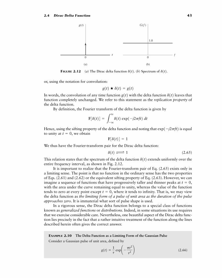
2.4 Dirac Delta Function 43
0
(a)
t
g(t)
0
1.0
(b)
f
G(f )
FIGURE 2.12 (a) The Dirac delta function (b) Spectrum of d1t2.d1t2.or, using the notation for convolution:
In words, the convolution of any time function with the delta function leaves thatfunction completely unchanged. We refer to this statement as the replication property ofthe delta function.
By definition, the Fourier transform of the delta function is given by
Hence, using the sifting property of the delta function and noting that is equalto unity at we obtain
We thus have the Fourier-transform pair for the Dirac delta function:
(2.65)
This relation states that the spectrum of the delta function extends uniformly over theentire frequency interval, as shown in Fig. 2.12.
It is important to realize that the Fourier-transform pair of Eq. (2.65) exists only ina limiting sense. The point is that no function in the ordinary sense has the two propertiesof Eqs. (2.61) and (2.62) or the equivalent sifting property of Eq. (2.63). However, we canimagine a sequence of functions that have progressively taller and thinner peaks at with the area under the curve remaining equal to unity, whereas the value of the functiontends to zero at every point except where it tends to infinity. That is, we may viewthe delta function as the limiting form of a pulse of unit area as the duration of the pulseapproaches zero. It is immaterial what sort of pulse shape is used.
In a rigorous sense, the Dirac delta function belongs to a special class of functionsknown as generalized functions or distributions. Indeed, in some situations its use requiresthat we exercise considerable care. Nevertheless, one beautiful aspect of the Dirac delta func-tion lies precisely in the fact that a rather intuitive treatment of the function along the linesdescribed herein often gives the correct answer.
EXAMPLE 2.10 The Delta Function as a Limiting Form of the Gaussian Pulse
Consider a Gaussian pulse of unit area, defined by
(2.66)g1t2 �1t
exp¢�pt2
t2≤
t � 0,
t � 0,
d1t2d1t2 Δ 1
F3d1t24 � 1t � 0,
exp1�j2pft2F3d1t24 � L
q
�qd1t2 exp1�j2pft2 dt
d1t2g1t2g1t2 � d1t2 � g1t2
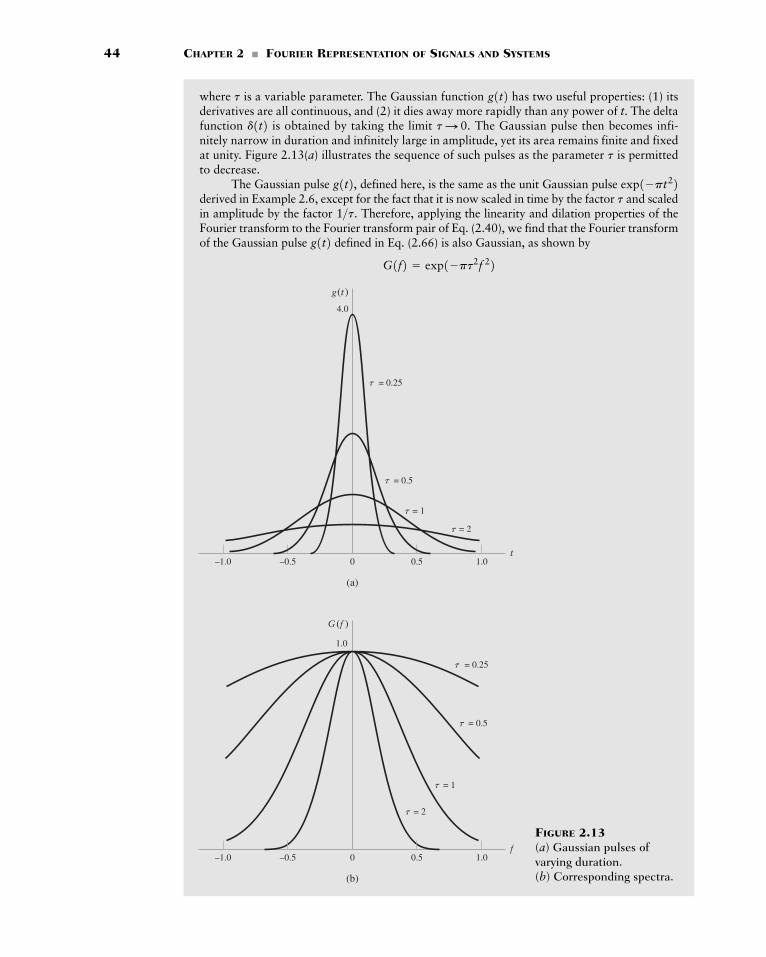
44 CHAPTER 2 � FOURIER REPRESENTATION OF SIGNALS AND SYSTEMS
0 0.5 1.0–0.5–1.0t
= 2�
= 1�
= 0.5�
= 0.25�
4.0
(a)
0 0.5 1.0–0.5–1.0f
(b)
1.0
g(t)
G(f )
= 2�
= 1�
= 0.5�
= 0.25�
FIGURE 2.13(a) Gaussian pulses ofvarying duration.(b) Corresponding spectra.
where is a variable parameter. The Gaussian function has two useful properties: (1) itsderivatives are all continuous, and (2) it dies away more rapidly than any power of t. The deltafunction is obtained by taking the limit The Gaussian pulse then becomes infi-nitely narrow in duration and infinitely large in amplitude, yet its area remains finite and fixedat unity. Figure 2.13(a) illustrates the sequence of such pulses as the parameter is permittedto decrease.
The Gaussian pulse defined here, is the same as the unit Gaussian pulse derived in Example 2.6, except for the fact that it is now scaled in time by the factor and scaledin amplitude by the factor Therefore, applying the linearity and dilation properties of theFourier transform to the Fourier transform pair of Eq. (2.40), we find that the Fourier transformof the Gaussian pulse defined in Eq. (2.66) is also Gaussian, as shown by
G1f2 � exp1�pt2f 22g1t2
1>t. t
exp1�pt22g1t2,t
tS 0.d1t2g1t2t
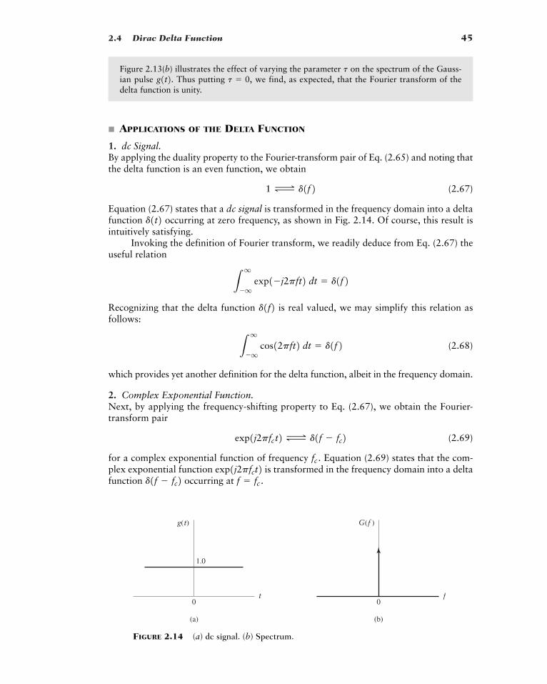
2.4 Dirac Delta Function 45
0
(b)
f
G(f )
0
1.0
(a)
t
g(t)
FIGURE 2.14 (a) dc signal. (b) Spectrum.
Figure 2.13(b) illustrates the effect of varying the parameter on the spectrum of the Gauss-ian pulse Thus putting we find, as expected, that the Fourier transform of thedelta function is unity.
� APPLICATIONS OF THE DELTA FUNCTION
1. dc Signal.By applying the duality property to the Fourier-transform pair of Eq. (2.65) and noting thatthe delta function is an even function, we obtain
(2.67)
Equation (2.67) states that a dc signal is transformed in the frequency domain into a deltafunction occurring at zero frequency, as shown in Fig. 2.14. Of course, this result isintuitively satisfying.
Invoking the definition of Fourier transform, we readily deduce from Eq. (2.67) theuseful relation
Recognizing that the delta function is real valued, we may simplify this relation asfollows:
(2.68)
which provides yet another definition for the delta function, albeit in the frequency domain.
2. Complex Exponential Function.Next, by applying the frequency-shifting property to Eq. (2.67), we obtain the Fourier-transform pair
(2.69)
for a complex exponential function of frequency Equation (2.69) states that the com-plex exponential function is transformed in the frequency domain into a deltafunction occurring at f � fc .d1f � fc2 exp1j2pfct2 fc .
exp1j2pfct2 Δ d1f � fc2
Lq
�q cos12pft2 dt � d1f2
d1f2L
q
�q exp1�j2pft2 dt � d1f2
d1t21 Δ d1f2
t � 0,g1t2. t
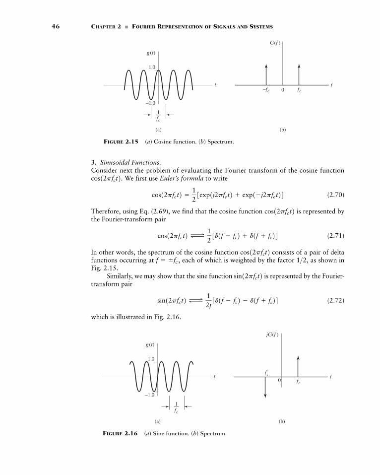
46 CHAPTER 2 � FOURIER REPRESENTATION OF SIGNALS AND SYSTEMS
—1fc
fc–fc
(a) (b)
g (t)
t
G(f )
f
–1.0
0
1.0
FIGURE 2.15 (a) Cosine function. (b) Spectrum.
—1fc
fc
–fc
(a) (b)
g (t)
t
jG(f )
f
–1.0
0
1.0
FIGURE 2.16 (a) Sine function. (b) Spectrum.
3. Sinusoidal Functions.Consider next the problem of evaluating the Fourier transform of the cosine function
We first use Euler’s formula to write
(2.70)
Therefore, using Eq. (2.69), we find that the cosine function is represented bythe Fourier-transform pair
(2.71)
In other words, the spectrum of the cosine function consists of a pair of deltafunctions occurring at each of which is weighted by the factor as shown inFig. 2.15.
Similarly, we may show that the sine function is represented by the Fourier-transform pair
(2.72)
which is illustrated in Fig. 2.16.
sin12pfct2 Δ12j3d1f � fc2 � d1f fc24
sin12pfct21>2,f � �fc ,
cos12pfct2cos12pfct2 Δ
123d1f � fc2 d1f fc24
cos12pfct2cos12pfct2 �
123exp1j2pfct2 exp1�j2pfct24
cos12pfct2.
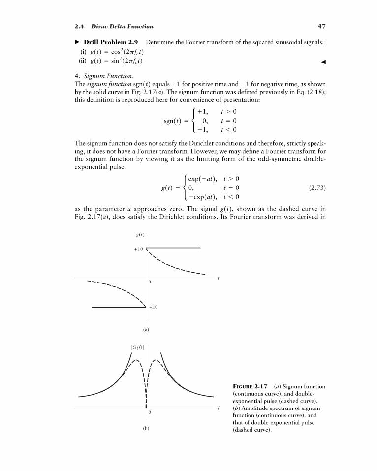
2.4 Dirac Delta Function 47
0
–1.0
t
+1.0
g(t)
0f
|G(f) |
(a)
(b)
FIGURE 2.17 (a) Signum function(continuous curve), and double-exponential pulse (dashed curve).(b) Amplitude spectrum of signumfunction (continuous curve), andthat of double-exponential pulse(dashed curve).
� Drill Problem 2.9 Determine the Fourier transform of the squared sinusoidal signals:
(i)(ii) �
4. Signum Function.The signum function equals for positive time and for negative time, as shownby the solid curve in Fig. 2.17(a). The signum function was defined previously in Eq. (2.18);this definition is reproduced here for convenience of presentation:
The signum function does not satisfy the Dirichlet conditions and therefore, strictly speak-ing, it does not have a Fourier transform. However, we may define a Fourier transform forthe signum function by viewing it as the limiting form of the odd-symmetric double-exponential pulse
(2.73)
as the parameter a approaches zero. The signal shown as the dashed curve inFig. 2.17(a), does satisfy the Dirichlet conditions. Its Fourier transform was derived in
g1t2,g1t2 � c exp1�at2, t � 0
0, t � 0�exp1at2, t � 0
sgn1t2 � c1, t � 00, t � 0
�1, t � 0
�11sgn1t2g1t2 � sin212pfc t2g1t2 � cos212pfc t2

48 CHAPTER 2 � FOURIER REPRESENTATION OF SIGNALS AND SYSTEMS
0
(b)
f
|G(f )|
0
1.0
12
—
(a)
t
g(t)
FIGURE 2.18 (a) Unit step function. (b) Amplitude spectrum.
Example 2.3; the result is given by [see Eq. (2.19)]:
The amplitude spectrum is shown as the dashed curve in Fig. 2.17(b). In the limitas a approaches zero, we have
That is,
(2.74)
The amplitude spectrum of the signum function is shown as the continuous curve inFig. 2.17(b). Here we see that for small a, the approximation is very good except near theorigin on the frequency axis. At the origin, the spectrum of the approximating function is zero for whereas the spectrum of the signum function goes to infinity.
5. Unit Step Function.The unit step function u(t) equals for positive time and zero for negative time. Previ-ously defined in Eq. (2.11), it is reproduced here for convenience:
The waveform of the unit step function is shown in Fig. 2.18(a). From this defining equa-tion and that of the signum function, or from the waveforms of Figs. 2.17(a) and 2.18(a),we see that the unit step function and signum function are related by
(2.75)
Hence, using the linearity property of the Fourier transform and the Fourier-transformpairs of Eqs. (2.67) and (2.75), we find that the unit step function is represented by theFourier-transform pair
u1t2 �123sgn11t2 124
u1t2 � d 1, t � 012
, t � 0
0, t � 0
1
a � 0,g1t2
sgn1t2 Δ1
jpf
�1
jpf
F3sgn1t24 � limaS0
�4jpf
a2 12pf22
ƒG1f2 ƒG1f2 �
�j4pf
a2 12pf22
2.4 Dirac Delta Function 49
(2.76)
This means that the spectrum of the unit step function contains a delta function weightedby a factor of and occurring at zero frequency, as shown in Fig. 2.18(b).
6. Integration in the Time Domain (Revisited).The relation of Eq. (2.41) describes the effect of integration on the Fourier transform of asignal assuming that is zero. We now consider the more general case, with nosuch assumption made.
Let
(2.77)
The integrated signal can be viewed as the convolution of the original signal andthe unit step function as shown by
where the time-shifted unit step function is itself defined by
Recognizing that convolution in the time domain is transformed into multiplication in thefrequency domain in accordance with Property 12, and using the Fourier-transform pairof Eq. (2.76) for the unit step function we find that the Fourier transform of is
(2.78)
where is the Fourier transform of According to the sifting property of a deltafunction formulated in the frequency domain, we have
Hence, we may rewrite Eq. (2.78) in the equivalent form:
In general, the effect of integrating the signal is therefore described by the Fourier-transform pair
(2.79)
This is the desired result, which includes Eq. (2.41) as a special case (i.e., ).
� Drill Problem 2.10 Consider the function
g1t2 � da t 12b � da t �
12b
G102 � 0
Lt
�qg1t2 dt Δ
1j2pf
G1f2 12
G102d1f2g1t2
Y1f2 �1
j2pfG1f2
12
G102d1f2
G1f2d1f2 � G102d1f2g1t2.G1f2
Y1f2 � G1f2c 1j2pf
12d1f2 d
y1t2u1t2,
u1t � t2 � d 1, t � t12
, t � t
0, t � t
u1t � t2y1t2 � L
q
�qg1t2u1t � t2 dt
u1t2, g1t2y1t2y1t2 � L
t
�qg1t2 dt
G102g1t2,
1>2u1t2 Δ
1j2pf
12d1f2
50 CHAPTER 2 � FOURIER REPRESENTATION OF SIGNALS AND SYSTEMS
which consists of the difference between two delta functions at The integration of
with respect to time t yields the unit rectangular function Using Eq. (2.79), show that
which is a special form of Eq. (2.10). �
2.5 Fourier Transforms of Periodic Signals
It is well known that by using the Fourier series, a periodic signal can be represented as asum of complex exponentials. (Appendix 2 presents a review of the Fourier series.) Also,in a limiting sense, Fourier transforms can be defined for complex exponentials, as demon-strated in Eqs. (2.69), (2.71), and (2.72). Therefore, it seems reasonable to represent a peri-odic signal in terms of a Fourier transform, provided that this transform is permitted toinclude delta functions.
Consider then a periodic signal where the subscript denotes the period ofthe signal. We know that can be represented in terms of the complex exponentialFourier series as (see Appendix 2)
(2.80)
where is the complex Fourier coefficient, defined by
(2.81)
and is the fundamental frequency defined as the reciprocal of the period that is,
(2.82)
Let be a pulselike function, which equals over one period and is zero elsewhere;that is,
(2.83)
The periodic signal may now be expressed in terms of the function as the infi-nite summation
(2.84)
Based on this representation, we may view as a generating function, in that it gener-ates the periodic signal Being pulselike with some finite energy, the function isFourier transformable. Accordingly, in light of Eqs. (2.82) and (2.83), we may rewrite theformula for the complex Fourier coefficient as follows:
(2.85)� f0G1nf02cn � f0L
q
�qg1t2 exp1�j2pnf0t2 dt
cn
g1t2gT01t2. g1t2
gT01t2 � a
q
m��qg1t � mT02
g1t2gT01t2
g1t2 � c gT01t2, �
T0
2� t �
T0
20, elsewhere
gT01t2g1t2
f0 �1T0
T0;f0
cn �1T0 L
T0>2�T0>2 gT0
1t2 exp1�j2pnf0t2 dt
cn
gT01t2 � a
q
n��qcn exp1j2pnf0t2
gT01t2 T0gT0
1t2,
rect1t2 Δ sinc1f2rect1t2.g1t2
t � �12
.
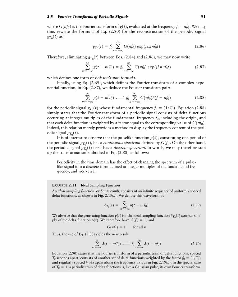
2.5 Fourier Transforms of Periodic Signals 51
where is the Fourier transform of evaluated at the frequency We maythus rewrite the formula of Eq. (2.80) for the reconstruction of the periodic signal
as
(2.86)
Therefore, eliminating between Eqs. (2.84) and (2.86), we may now write
(2.87)
which defines one form of Poisson’s sum formula.Finally, using Eq. (2.69), which defines the Fourier transform of a complex expo-
nential function, in Eq. (2.87), we deduce the Fourier-transform pair:
(2.88)
for the periodic signal whose fundamental frequency Equation (2.88)simply states that the Fourier transform of a periodic signal consists of delta functionsoccurring at integer multiples of the fundamental frequency including the origin, andthat each delta function is weighted by a factor equal to the corresponding value of Indeed, this relation merely provides a method to display the frequency content of the peri-odic signal
It is of interest to observe that the pulselike function constituting one period ofthe periodic signal has a continuous spectrum defined by On the other hand,the periodic signal itself has a discrete spectrum. In words, we may therefore sumup the transformation embodied in Eq. (2.88) as follows:
Periodicity in the time domain has the effect of changing the spectrum of a pulse-like signal into a discrete form defined at integer multiples of the fundamental fre-quency, and vice versa.
EXAMPLE 2.11 Ideal Sampling Function
An ideal sampling function, or Dirac comb, consists of an infinite sequence of uniformly spaceddelta functions, as shown in Fig. 2.19(a). We denote this waveform by
(2.89)
We observe that the generating function for the ideal sampling function consists sim-ply of the delta function We therefore have and
Thus, the use of Eq. (2.88) yields the new result
(2.90)
Equation (2.90) states that the Fourier transform of a periodic train of delta functions, spacedseconds apart, consists of another set of delta functions weighted by the factor
and regularly spaced Hz apart along the frequency axis as in Fig. 2.19(b). In the special caseof a periodic train of delta functions is, like a Gaussian pulse, its own Fourier transform.T0 � 1,
f0f0 � 11>T02T0
aq
m��qd1t � mT02 Δ f0 a
q
n��qd1f � nf02
G1nf02 � 1 for all n
G1f2 � 1,d1t2. dT01t2g1t2
dT01t2 � a
q
m��qd1t � mT02
gT01t2 G1f2.gT01t2, g1t2,gT0
1t2.G1nf02.f0,
f0 � 11>T02.gT01t2
aq
m��qg1t � mT02 Δ f0 a
q
n��qG1nf02d1f � nf02
aq
m��qg1t � mT02 � f0 a
q
n��qG1nf02 exp1j2pnf0t2
gT01t2gT01t2 � f0 a
q
n��qG1nf02 exp1j2pnf0t2
gT01t2
f � nf0.g1t2,G1nf02
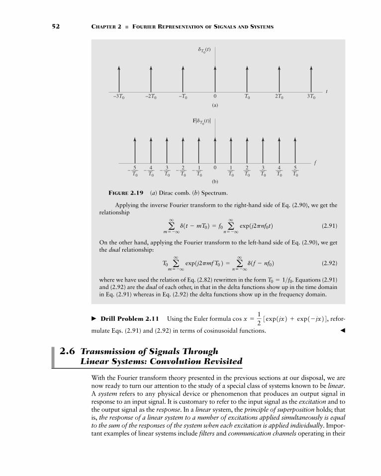
52 CHAPTER 2 � FOURIER REPRESENTATION OF SIGNALS AND SYSTEMS
Applying the inverse Fourier transform to the right-hand side of Eq. (2.90), we get therelationship
(2.91)
On the other hand, applying the Fourier transform to the left-hand side of Eq. (2.90), we getthe dual relationship:
(2.92)
where we have used the relation of Eq. (2.82) rewritten in the form Equations (2.91)and (2.92) are the dual of each other, in that in the delta functions show up in the time domainin Eq. (2.91) whereas in Eq. (2.92) the delta functions show up in the frequency domain.
� Drill Problem 2.11 Using the Euler formula refor-
mulate Eqs. (2.91) and (2.92) in terms of cosinusoidal functions. �
2.6 Transmission of Signals Through Linear Systems: Convolution Revisited
With the Fourier transform theory presented in the previous sections at our disposal, we arenow ready to turn our attention to the study of a special class of systems known to be linear.A system refers to any physical device or phenomenon that produces an output signal inresponse to an input signal. It is customary to refer to the input signal as the excitation and tothe output signal as the response. In a linear system, the principle of superposition holds; thatis, the response of a linear system to a number of excitations applied simultaneously is equalto the sum of the responses of the system when each excitation is applied individually. Impor-tant examples of linear systems include filters and communication channels operating in their
cos x �123exp1jx2 exp1�jx24,
T0 � 1>f0.
T0 aq
m��q exp1j2pmf T02 � a
q
n��qd1f � nf02
aq
m��qd1t � mT02 � f0 a
q
n��q exp1j2pnf0t2
0
(a)
�T0(t)
–T0–2T0–3T0 3T0T0 2T0
t
0
(b)
F|�T0(t)|
f—–– 1T0
—–1T0
—–2T0
—–3T0
—–4T0
—–5T0
—–– 2T0
—–– 3T0
—–– 4T0
—–– 5T0
FIGURE 2.19 (a) Dirac comb. (b) Spectrum.
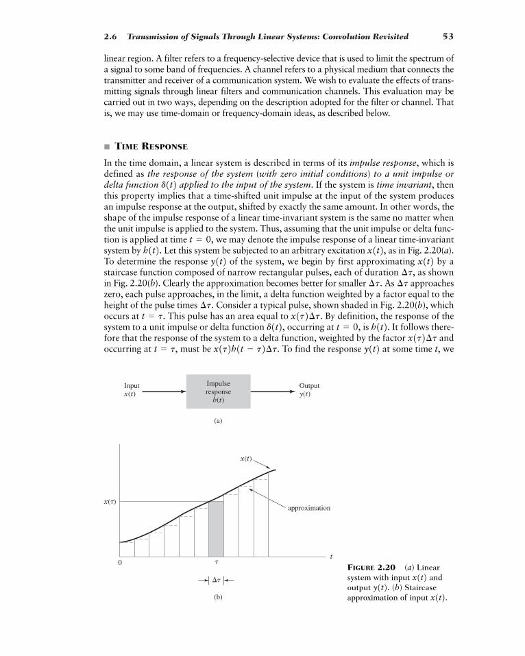
2.6 Transmission of Signals Through Linear Systems: Convolution Revisited 53
linear region. A filter refers to a frequency-selective device that is used to limit the spectrum ofa signal to some band of frequencies. A channel refers to a physical medium that connects thetransmitter and receiver of a communication system. We wish to evaluate the effects of trans-mitting signals through linear filters and communication channels. This evaluation may becarried out in two ways, depending on the description adopted for the filter or channel. Thatis, we may use time-domain or frequency-domain ideas, as described below.
� TIME RESPONSE
In the time domain, a linear system is described in terms of its impulse response, which isdefined as the response of the system (with zero initial conditions) to a unit impulse ordelta function applied to the input of the system. If the system is time invariant, thenthis property implies that a time-shifted unit impulse at the input of the system producesan impulse response at the output, shifted by exactly the same amount. In other words, theshape of the impulse response of a linear time-invariant system is the same no matter whenthe unit impulse is applied to the system. Thus, assuming that the unit impulse or delta func-tion is applied at time we may denote the impulse response of a linear time-invariantsystem by Let this system be subjected to an arbitrary excitation as in Fig. 2.20(a).To determine the response of the system, we begin by first approximating by astaircase function composed of narrow rectangular pulses, each of duration as shownin Fig. 2.20(b). Clearly the approximation becomes better for smaller As approacheszero, each pulse approaches, in the limit, a delta function weighted by a factor equal to theheight of the pulse times Consider a typical pulse, shown shaded in Fig. 2.20(b), whichoccurs at This pulse has an area equal to By definition, the response of thesystem to a unit impulse or delta function occurring at is It follows there-fore that the response of the system to a delta function, weighted by the factor andoccurring at must be To find the response at some time t, wey1t2x1t2h1t � t2¢t.t � t,
x1t2¢th1t2.t � 0,d1t2, x1t2¢t.t � t.¢t.
¢t¢t.¢t,
x1t2y1t2 x1t2,h1t2. t � 0,
d1t2
(b)
(a)
Outputy(t)
��
�
Inputx(t)
Impulseresponse
h(t)
x(t)
x(�)approximation
0t
FIGURE 2.20 (a) Linearsystem with input andoutput (b) Staircaseapproximation of input x1t2.y1t2. x1t2
54 CHAPTER 2 � FOURIER REPRESENTATION OF SIGNALS AND SYSTEMS
apply the principle of superposition. Thus, summing the various infinitesimal responsesdue to the various input pulses, we obtain in the limit, as approaches zero,
(2.93)
This relation is called the convolution integral.In Eq. (2.93), three different time scales are involved: excitation time response time
t, and system-memory time This relation is the basis of time-domain analysis oflinear time-invariant systems. It states that the present value of the response of a lineartime-invariant system is a weighted integral over the past history of the input signal,weighted according to the impulse response of the system. Thus, the impulse response actsas a memory function for the system.
In Eq. (2.93), the excitation is convolved with the impulse response to pro-duce the response Since convolution is commutative, it follows that we may also write
(2.94)
where is convolved with
EXAMPLE 2.12 Tapped-Delay-Line Filter
Consider a linear time-invariant filter with impulse response We make two assumptions:
1. Causality, which means that the impulse response is zero for 2. Finite support, which means that the impulse response of the filter is of some finite dura-
tion so that we may write for
Under these two assumptions, we may express the filter output produced in response tothe input as
(2.95)
Let the input impulse response and output be uniformly sampled at the ratesamples per second, so that we may put
and
where k and n are integers, and is the sampling period. Assuming that is small enoughfor the product to remain essentially constant for forall values of k and we may approximate Eq. (2.95) by a convolution sum as shown by
where Define the weight
(2.96)
We may then rewrite the formula for as
(2.97)y1n ¢t2 � aN�1
k�0wkx1n ¢t � k ¢t2
y1n ¢t2wk � h1k ¢t2 ¢t, k � 0, 1, Á , N � 1
N ¢t � Tf .
y1n ¢t2 � aN�1
k�0h1k ¢t2x1n ¢t � k ¢t2 ¢t
t,k ¢t � t � 1k 12 ¢th1t2x1t � t2 ¢t¢t
t � k ¢t
t � n ¢t11>¢t2 y1t2h1t2,x1t2,
y1t2 � LTf
0h1t2x1t � t2 dt
x1t2 y1t2t � Tf .h1t2 � 0Tf ,
t � 0.h1t2h1t2.
x1t2.h1t2y1t2 � L
q
�qh1t2x1t � t2 dt
y1t2. h1t2x1t2
1t � t2. t,
y1t2 � Lq
�qx1t2h1t � t2 dt
¢t
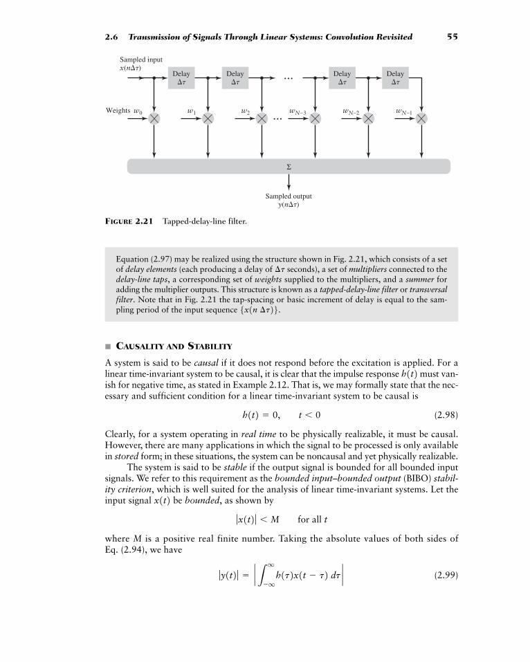
2.6 Transmission of Signals Through Linear Systems: Convolution Revisited 55
wN–2 wN–1
Delay��
Sampled inputx(n��)
Sampled outputy(n��)
Weights
Σ
w0 w1 w2
Delay��
Delay��
wN–3
Delay��
...
...
FIGURE 2.21 Tapped-delay-line filter.
Equation (2.97) may be realized using the structure shown in Fig. 2.21, which consists of a setof delay elements (each producing a delay of seconds), a set of multipliers connected to thedelay-line taps, a corresponding set of weights supplied to the multipliers, and a summer foradding the multiplier outputs. This structure is known as a tapped-delay-line filter or transversalfilter. Note that in Fig. 2.21 the tap-spacing or basic increment of delay is equal to the sam-pling period of the input sequence
� CAUSALITY AND STABILITY
A system is said to be causal if it does not respond before the excitation is applied. For alinear time-invariant system to be causal, it is clear that the impulse response must van-ish for negative time, as stated in Example 2.12. That is, we may formally state that the nec-essary and sufficient condition for a linear time-invariant system to be causal is
(2.98)
Clearly, for a system operating in real time to be physically realizable, it must be causal.However, there are many applications in which the signal to be processed is only availablein stored form; in these situations, the system can be noncausal and yet physically realizable.
The system is said to be stable if the output signal is bounded for all bounded inputsignals. We refer to this requirement as the bounded input–bounded output (BIBO) stabil-ity criterion, which is well suited for the analysis of linear time-invariant systems. Let theinput signal be bounded, as shown by
where M is a positive real finite number. Taking the absolute values of both sides ofEq. (2.94), we have
(2.99)ƒy1t2 ƒ � ` Lq
�qh1t2x1t � t2 dt `
ƒx1t2 ƒ � M for all t
x1t2
h1t2 � 0, t � 0
h1t2
5x1n ¢t26.
¢t
56 CHAPTER 2 � FOURIER REPRESENTATION OF SIGNALS AND SYSTEMS
Next, we recognize that the absolute value of an integral is bounded by the integral of theabsolute value of the integrand, as shown by
Hence, substituting this inequality into Eq. (2.99) yields the important result
It follows therefore that for a linear time-invariant system to be stable, the impulse responsemust be absolutely integrable. That is, the necessary and sufficient condition for BIBO
stability of a linear time-invariant system is described by
(2.100)
where is the impulse response of the system.
� FREQUENCY RESPONSE
Consider next a linear time-invariant system of impulse response which is driven bya complex exponential input of unit amplitude and frequency that is,
(2.101)
Using Eqs. (2.101) in (2.94), the response of the system is obtained as
(2.102)
Define the transfer function or frequency response of the system as the Fourier transformof its impulse response, as shown by
(2.103)
The terms transfer function and frequency response are used interchangably. The integralin the last line of Eq. (2.102) is the same as that of Eq. (2.103), except for the fact that is used in place of t. Hence, we may rewrite Eq. (2.102) in the form
(2.104)
Equation (2.104) states that the response of a linear time-invariant system to a complexexponential function of frequency is the same complex exponential function multipliedby a constant coefficient H1f2. f
y1t2 � H1f2 exp1j2pft2t
H1f2 � Lq
�qh1t2 exp1�j2pft2 dt
� exp1j2pft2Lq
�qh1t2 exp1�j2pft2 dt
y1t2 � Lq
�qh1t2 exp3j2pf1t � t24 dt
x1t2 � exp1j2pft2f;
h1t2,
h1t2L
q
�qƒh1t2 ƒ dt � �
h1t2
ƒy1t2 ƒ � MLq
�qƒh1t2 ƒ dt
� MLq
�qƒh1t2 ƒ dt
` Lq
�qh1t2x1t � t2 dt ` �L
q
�qƒh1t2x1t � t2 ƒ dt
2.6 Transmission of Signals Through Linear Systems: Convolution Revisited 57
Equation (2.103) is one definition of the transfer function An alternative defi-nition of the transfer function may be deduced by dividing Eq. (2.104) by (2.101) to obtain
(2.105)
Consider next an arbitrary signal applied to the system. The signal may beexpressed in terms of its inverse Fourier transform as
(2.106)
Equivalently, we may express in the limiting form
(2.107)
That is, the input signal may be viewed as a superposition of complex exponentialsof incremental amplitude. Because the system is linear, the response to this superpositionof complex exponential inputs is given by
(2.108)
The Fourier transform of the output signal is therefore readily obtained as
(2.109)
According to Eq. (2.109), a linear time-invariant system may thus be described quite sim-ply in the frequency domain by noting that the Fourier transform of the output is equal tothe product of the frequency response of the system and the Fourier transform of the input.
Of course, we could have deduced the result of Eq. (2.109) directly by recognizing twofacts:
1. The response of a linear time-invariant system of impulse response to an arbi-trary input is obtained by convolving with in accordance withEq. (2.93).
2. The convolution of a pair of time functions is transformed into the multiplication oftheir Fourier transforms.
The alternative derivation of Eq. (2.109) above is presented primarily to develop an under-standing of why the Fourier representation of a time function as a superposition of com-plex exponentials is so useful in analyzing the behavior of linear time-invariant systems.
The frequency response is a characteristic property of a linear time-invariant sys-tem. It is, in general, a complex quantity, so that we may express it in the form
(2.110)
where is called the amplitude response or magnitude response, and the phaseor phase response. In the special case of a linear system with real-valued impulse response
the frequency response exhibits conjugate symmetry, which means that
ƒH1f2 ƒ � ƒH1�f2 ƒH1f2h1t2,
b1f2ƒH1f2 ƒH1f2 � ƒH1f2 ƒ exp3jb1f24
H1f2
h1t2,x1t2x1t2 h1t2y1t2
Y1f2 � H1f2X1f2y1t2
�Lq
�qH1f2X1f2 exp1j2pft2 df
y1t2 � lim¢fS0
f � k ¢f
aq
k��qH1f2X1f2 exp1j2pft2 ¢f
x1t2x1t2 � lim
¢fS0f � k ¢f
aq
k��qX1f2 exp1j2pft2 ¢f
x1t2x1t2 �L
q
�qX1f2 exp1j2pft2 df
x1t2x1t2H1f2 �
y1t2x1t2 ` x1t2�exp1j2pft2
H1f2.
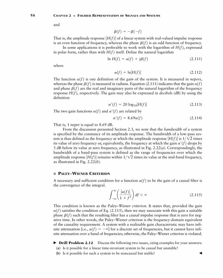
58 CHAPTER 2 � FOURIER REPRESENTATION OF SIGNALS AND SYSTEMS
and
That is, the amplitude response of a linear system with real-valued impulse responseis an even function of frequency, whereas the phase is an odd function of frequency.
In some applications it is preferable to work with the logarithm of expressedin polar form, rather than with itself. Define the natural logarithm
(2.111)
where
(2.112)
The function is one definition of the gain of the system. It is measured in nepers,whereas the phase is measured in radians. Equation (2.111) indicates that the gain and phase are the real and imaginary parts of the natural logarithm of the frequencyresponse respectively. The gain may also be expressed in decibels (dB) by using thedefinition
(2.113)
The two gain functions and are related by
(2.114)
That is, 1 neper is equal to 8.69 dB.From the discussion presented Section 2.3, we note that the bandwidth of a system
is specified by the constancy of its amplitude response. The bandwidth of a low-pass sys-tem is thus defined as the frequency at which the amplitude response is timesits value of zero frequency or, equivalently, the frequency at which the gain drops by3 dB below its value at zero frequency, as illustrated in Fig. 2.22(a). Correspondingly, thebandwidth of a band-pass system is defined as the range of frequencies over which theamplitude response remains within times its value at the mid-band frequency,as illustrated in Fig. 2.22(b).
� PALEY–WIENER CRITERION
A necessary and sufficient condition for a function to be the gain of a causal filter isthe convergence of the integral.
(2.115)
This condition is known as the Paley–Wiener criterion. It states that, provided the gainsatisfies the condition of Eq. (2.115), then we may associate with this gain a suitable
phase such that the resulting filter has a causal impulse response that is zero for neg-ative time. In other words, the Paley–Wiener criterion is the frequency-domain equivalentof the causality requirement. A system with a realizable gain characteristic may have infi-nite attenuation [i.e., ] for a discrete set of frequencies, but it cannot have infi-nite attenuation over a band of frequencies; otherwise, the Paley–Wiener criterion is violated.
� Drill Problem 2.12 Discuss the following two issues, citing examples for your answers:(a) Is it possible for a linear time-invariant system to be causal but unstable?(b) Is it possible for such a system to be noncausal but stable? �
a1f2 � ��
b1f2a1f2L
q
�q¢ ƒa1f2 ƒ
1 f 2 ≤ df � �
a1f2
1>12ƒH1f2 ƒa�1f21>12ƒH1f2 ƒ
a�1f2 � 8.69a1f2a�1f2a1f2a�1f2 � 20 log10 ƒH1f2 ƒ
H1f2,b1f2 a1f2b1f2a1f2a1f2 � ln ƒH1f2 ƒ
ln H1f2 � a1f2 jb1f2H1f2 H1f2,b1f2ƒH1f2 ƒb1f2 � �b1�f2
2.6 Transmission of Signals Through Linear Systems: Convolution Revisited 59
(a)
–B Bf
|H(f )|
|H(0)|
|H(0)|———
0
/2
(b)
–fc – B –fc + B
–fc
f
|H(f )|
|H(fc)|
|H(fc)|———
0
/2
fc – B fc + B
fc
FIGURE 2.22 Illustration of the definition of system bandwidth.(a) Low-pass system. (b) Band-pass system.
� Drill Problem 2.13 The impulse response of a linear system is defined by the Gaussianfunction
where is an adjustable parameter that defines pulse duration. Determine the frequency responseof the system. �
� Drill Problem 2.14 A tapped-delay-line filter consists of N weights, where N is odd. Itis symmetric with respect to the center tap; that is, the weights satisfy the condition
(a) Find the amplitude response of the filter.
(b) Show that this filter has a linear phase response. What is the implication of this property?(c) What is the time delay produced by the filter? �
wn � wN�1�n , 0 � n � N � 1
t
h1t2 � exp¢�t2
2t2 ≤
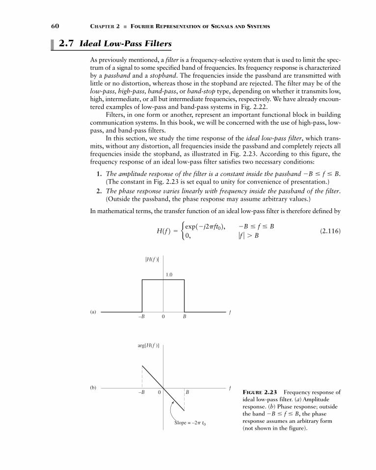
60 CHAPTER 2 � FOURIER REPRESENTATION OF SIGNALS AND SYSTEMS
2.7 Ideal Low-Pass Filters
As previously mentioned, a filter is a frequency-selective system that is used to limit the spec-trum of a signal to some specified band of frequencies. Its frequency response is characterizedby a passband and a stopband. The frequencies inside the passband are transmitted withlittle or no distortion, whereas those in the stopband are rejected. The filter may be of thelow-pass, high-pass, band-pass, or band-stop type, depending on whether it transmits low,high, intermediate, or all but intermediate frequencies, respectively. We have already encoun-tered examples of low-pass and band-pass systems in Fig. 2.22.
Filters, in one form or another, represent an important functional block in buildingcommunication systems. In this book, we will be concerned with the use of high-pass, low-pass, and band-pass filters.
In this section, we study the time response of the ideal low-pass filter, which trans-mits, without any distortion, all frequencies inside the passband and completely rejects allfrequencies inside the stopband, as illustrated in Fig. 2.23. According to this figure, thefrequency response of an ideal low-pass filter satisfies two necessary conditions:
1. The amplitude response of the filter is a constant inside the passband(The constant in Fig. 2.23 is set equal to unity for convenience of presentation.)
2. The phase response varies linearly with frequency inside the passband of the filter.(Outside the passband, the phase response may assume arbitrary values.)
In mathematical terms, the transfer function of an ideal low-pass filter is therefore defined by
(2.116)H1f2 � b exp1�j2pft02, �B � f � B0, ƒf ƒ � B
�B � f � B.
0(a)
1.0
f
|H(f )|
–B B
0(b)
Slope = –2� t0
f
arg[H(f )]
–B B FIGURE 2.23 Frequency response ofideal low-pass filter. (a) Amplituderesponse. (b) Phase response; outsidethe band the phaseresponse assumes an arbitrary form(not shown in the figure).
�B � f � B,
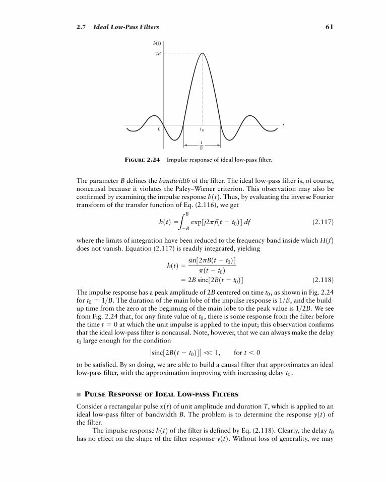
2.7 Ideal Low-Pass Filters 61
0
h(t)
2B
1B
tt 0
FIGURE 2.24 Impulse response of ideal low-pass filter.
The parameter B defines the bandwidth of the filter. The ideal low-pass filter is, of course,noncausal because it violates the Paley–Wiener criterion. This observation may also beconfirmed by examining the impulse response Thus, by evaluating the inverse Fouriertransform of the transfer function of Eq. (2.116), we get
(2.117)
where the limits of integration have been reduced to the frequency band inside which does not vanish. Equation (2.117) is readily integrated, yielding
(2.118)
The impulse response has a peak amplitude of centered on time as shown in Fig. 2.24for The duration of the main lobe of the impulse response is and the build-up time from the zero at the beginning of the main lobe to the peak value is We seefrom Fig. 2.24 that, for any finite value of there is some response from the filter beforethe time at which the unit impulse is applied to the input; this observation confirmsthat the ideal low-pass filter is noncausal. Note, however, that we can always make the delay
large enough for the condition
to be satisfied. By so doing, we are able to build a causal filter that approximates an ideallow-pass filter, with the approximation improving with increasing delay
� PULSE RESPONSE OF IDEAL LOW-PASS FILTERS
Consider a rectangular pulse of unit amplitude and duration T, which is applied to anideal low-pass filter of bandwidth B. The problem is to determine the response ofthe filter.
The impulse response of the filter is defined by Eq. (2.118). Clearly, the delay has no effect on the shape of the filter response . Without loss of generality, we mayy1t2 t0h1t2
y1t2x1t2
t0.
ƒsinc32B1t � t024 ƒ V 1, for t � 0
t0
t � 0t0,
1>2B.1>B,t0 � 1>B.
t0,2B
� 2B sinc32B1t � t024h1t2 �
sin32pB1t � t024p1t � t02
H1f2h1t2 �L
B
�B exp3j2pf1t � t024 df
h1t2.

62 CHAPTER 2 � FOURIER REPRESENTATION OF SIGNALS AND SYSTEMS
therefore simplify the exposition by setting in which case the impulse response ofEq. (2.118) reduces to
(2.119)
With the input for the resulting response of the filter isgiven by the convolution integral
(2.120)
Define a new dimensionless variable
Then, changing the integration variable from to we may rewrite Eq. (2.120) as
(2.121)
In Eq. (2.121), we have introduced a new expression called the sine integral, which isdefined by
(2.122)
Unfortunately, the sine integral Si(u) cannot be evaluated in closed form in terms of ele-mentary functions. However, it can be integrated in a power series, which, in turn, leadsto the graph plotted in Fig. 2.25. From this figure we make three observations:
1. The sine integral is an oscillatory function of u, having odd symmetry about theorigin
2. It has its maxima and minima at multiples of 3. It approaches the limiting value for large positive values of u.
In Fig. 2.25, we see that the sine integral oscillates at a frequency of Corre-spondingly, the filter response will also oscillate at a frequency equal to the cutoff fre-quency (i.e., bandwidth) B of the low-pass filter, as indicated in Fig. 2.26. The maximumvalue of occurs at and is equal to
We may show that the filter response has maxima and minima at
tmax � �T2
�1
2B
y1t21.8519 � 11.1792 ap
2b
umax � pSi1u2y1t2 1>2p.Si1u2
1p>22 p.u � 0.
Si1u2
Si1u2 �Lu
0
sin xx
dx
�1p5Si32pB1t T>224 � Si32pB1t � T>2246
�1pcL
2pB1tT>220
a sin llb dl � L
2pB1t�T>220
a sin llb dl d
y1t2 �1p L
2pB1tT>222pB1t�T>22 a
sin llb dl
l,t
l � 2pB1t � t2
� 2BLT>2
�T>2 asin32pB1t � t24
2pB1t � t2 b dt
� 2BLT>2
�T>2 sinc32B1t � t24 dt
y1t2 �Lq
�qx1t2h1t � t2 dt
�1T>22 � t � 1T>22,x1t2 � 1
h1t2 � 2B sinc12Bt2t0 � 0,
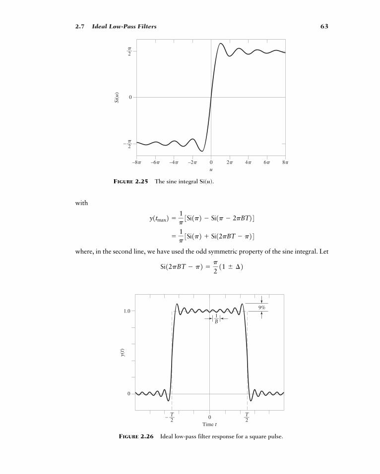
2.7 Ideal Low-Pass Filters 63
–8� –6� –4� –2� 0u
2� 4� 6� 8�
0
Si(u
)
– —�2
—�2
FIGURE 2.25 The sine integral Si(u).
9%
—1B
– —T2
—T20
Time t
0
1.0
y(t)
with
where, in the second line, we have used the odd symmetric property of the sine integral. Let
Si12pBT � p2 �p
211 � ¢2
�1p3Si1p2 Si12pBT � p24
y1tmax2 �1p3Si1p2 � Si1p � 2pBT24
FIGURE 2.26 Ideal low-pass filter response for a square pulse.
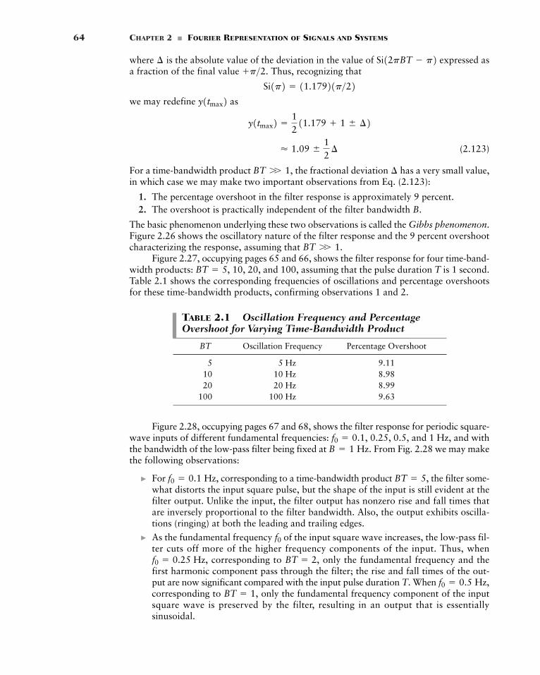
64 CHAPTER 2 � FOURIER REPRESENTATION OF SIGNALS AND SYSTEMS
where is the absolute value of the deviation in the value of expressed asa fraction of the final value Thus, recognizing that
we may redefine as
(2.123)
For a time-bandwidth product the fractional deviation has a very small value,in which case we may make two important observations from Eq. (2.123):
1. The percentage overshoot in the filter response is approximately 9 percent.2. The overshoot is practically independent of the filter bandwidth B.
The basic phenomenon underlying these two observations is called the Gibbs phenomenon.Figure 2.26 shows the oscillatory nature of the filter response and the 9 percent overshootcharacterizing the response, assuming that
Figure 2.27, occupying pages 65 and 66, shows the filter response for four time-band-width products: 10, 20, and 100, assuming that the pulse duration T is 1 second.Table 2.1 shows the corresponding frequencies of oscillations and percentage overshootsfor these time-bandwidth products, confirming observations 1 and 2.
BT � 5,
BT W 1.
¢BT W 1,
� 1.09 �12¢
y1tmax2 �1211.179 1 � ¢2
y1tmax2Si1p2 � 11.17921p>22
p>2.Si12pBT � p2¢
TABLE 2.1 Oscillation Frequency and PercentageOvershoot for Varying Time-Bandwidth Product
BT Oscillation Frequency Percentage Overshoot
5 5 Hz 9.1110 10 Hz 8.9820 20 Hz 8.99
100 100 Hz 9.63
Figure 2.28, occupying pages 67 and 68, shows the filter response for periodic square-wave inputs of different fundamental frequencies: 0.25, 0.5, and 1 Hz, and withthe bandwidth of the low-pass filter being fixed at From Fig. 2.28 we may makethe following observations:
� For corresponding to a time-bandwidth product the filter some-what distorts the input square pulse, but the shape of the input is still evident at thefilter output. Unlike the input, the filter output has nonzero rise and fall times thatare inversely proportional to the filter bandwidth. Also, the output exhibits oscilla-tions (ringing) at both the leading and trailing edges.
� As the fundamental frequency of the input square wave increases, the low-pass fil-ter cuts off more of the higher frequency components of the input. Thus, when
corresponding to only the fundamental frequency and thefirst harmonic component pass through the filter; the rise and fall times of the out-put are now significant compared with the input pulse duration T. When corresponding to only the fundamental frequency component of the inputsquare wave is preserved by the filter, resulting in an output that is essentiallysinusoidal.
BT � 1,f0 � 0.5 Hz,
BT � 2,f0 � 0.25 Hz,
f0
BT � 5,f0 � 0.1 Hz,
B � 1 Hz.f0 � 0.1,
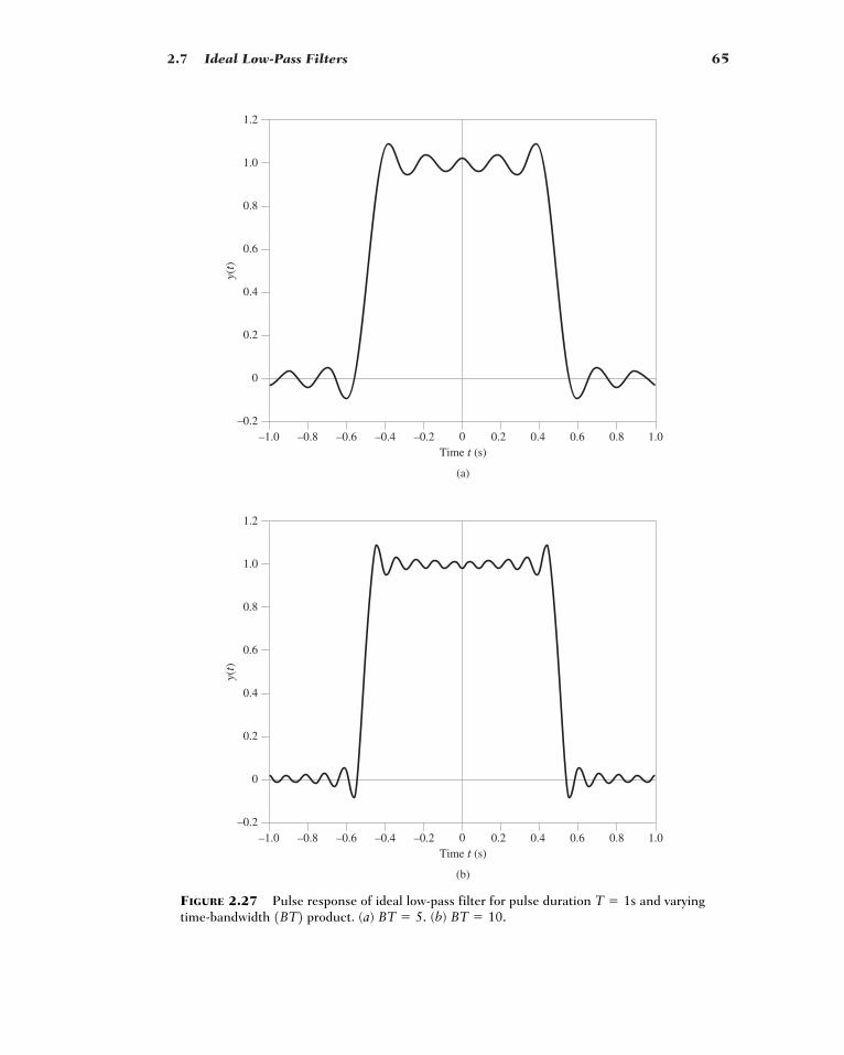
2.7 Ideal Low-Pass Filters 65
0Time t (s)
(a)
0.2
–1.0 –0.8 –0.6 –0.4 –0.2 0.2 0.4 0.6 0.8 1.0–0.2
0
0.4
0.6
0.8
1.0
1.2
y(t)
0Time t (s)
(b)
0.2
–1.0 –0.8 –0.6 –0.4 –0.2 0.2 0.4 0.6 0.8 1.0–0.2
0
0.4
0.6
0.8
1.0
1.2
y(t)
FIGURE 2.27 Pulse response of ideal low-pass filter for pulse duration and varyingtime-bandwidth product. (a) (b) BT � 10.BT � 5.1BT2 T � 1s
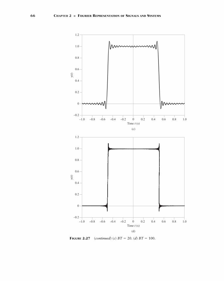
66 CHAPTER 2 � FOURIER REPRESENTATION OF SIGNALS AND SYSTEMS
0Time t (s)
(c)
0.2
–1.0 –0.8 –0.6 –0.4 –0.2 0.2 0.4 0.6 0.8 1.0–0.2
0
0.4
0.6
0.8
1.0
1.2
y(t)
0Time t (s)
(d)
0.2
–1.0 –0.8 –0.6 –0.4 –0.2 0.2 0.4 0.6 0.8 1.0–0.2
0
0.4
0.6
0.8
1.0
1.2
y(t)
FIGURE 2.27 (continued) (c) . (d) BT � 100.BT � 20
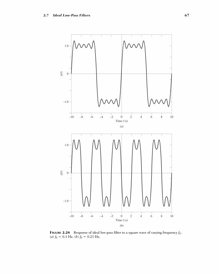
2.7 Ideal Low-Pass Filters 67
0Time t (s)
(a)
–10 –8 –6 –4 –2 2 4 6 8 10
–1.0
0
1.0
y(t)
0Time t (s)
(b)
–10 –8 –6 –4 –2 2 4 6 8 10
–1.0
0
1.0
y(t)
FIGURE 2.28 Response of ideal low-pass filter to a square wave of varying frequency (a) (b) f0 � 0.25 Hz.f0 � 0.1 Hz.
f0.
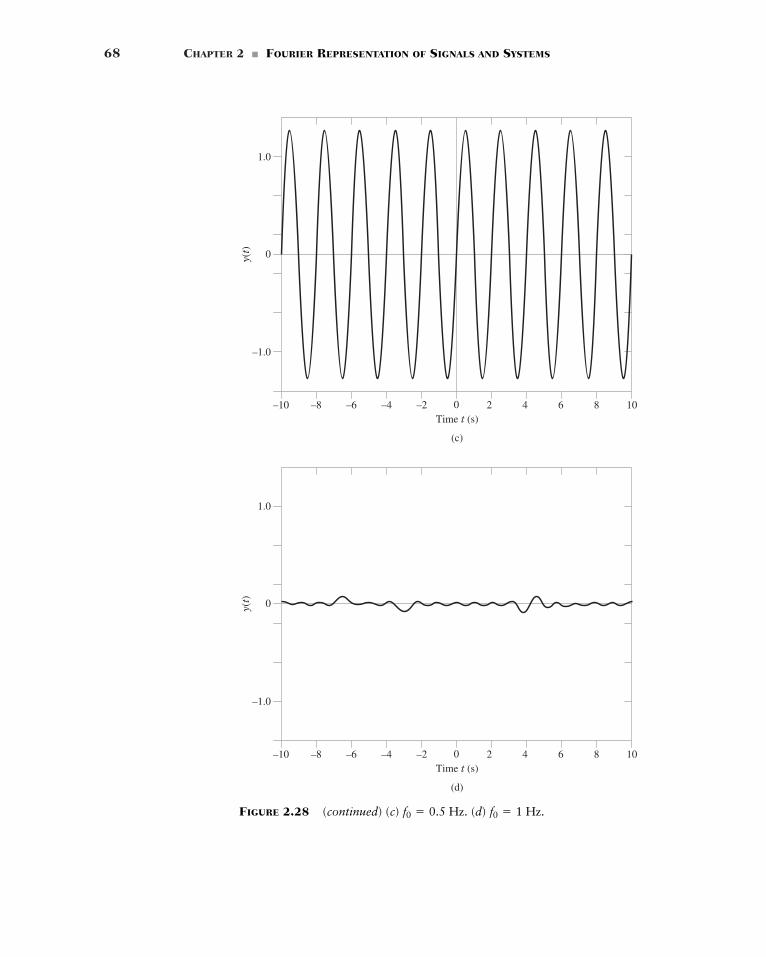
68 CHAPTER 2 � FOURIER REPRESENTATION OF SIGNALS AND SYSTEMS
0Time t (s)
(c)
–10 –8 –6 –4 –2 2 4 6 8 10
–1.0
0
1.0
y(t)
0Time t (s)
(d)
–10 –8 –6 –4 –2 2 4 6 8 10
–1.0
0
1.0
y(t)
FIGURE 2.28 (continued) (c) (d) f0 � 1 Hz.f0 � 0.5 Hz.
2.7 Ideal Low-Pass Filters 69
� When the fundamental frequency of the input square wave is increased further to thehigh value which corresponds to a time-bandwidth product , thedc component becomes the dominant output, and the shape of the input square waveis completely destroyed by the filter.
From these results, we draw an important conclusion: When using an ideal low-pass filter,we must use a time-bandwidth product to ensure that the waveform of the filterinput is recognizable from the resulting output. A value of BT greater than unity tends toreduce the rise time as well as decay time of the filter pulse response.
� APPROXIMATION OF IDEAL LOW-PASS FILTERS
A filter may be characterized by specifying its impulse response or, equivalently, itstransfer function . However, the application of a filter usually involves the separationof signals on the basis of their spectra (i.e., frequency contents). This, in turn, means thatthe design of filters is usually carried out in the frequency domain. There are two basicsteps involved in the design of a filter:
1. The approximation of a prescribed frequency response (i.e., amplitude response,phase response, or both) by a realizable transfer function.
2. The realization of the approximating transfer function by a physical device.
For an approximating transfer function to be physically realizable, it must representa stable system. Stability is defined here on the basis of the bounded input-bounded out-put criterion described in Eq. (2.100) that involves the impulse response . To specifythe corresponding condition for stability in terms of the transfer function, the traditionalapproach is to replace with s and recast the transfer function in terms of s. The newvariable s is permitted to have a real part as well as an imaginary part. Accordingly, we referto s as the complex frequency. Let denote the transfer function of the system, definedin the manner described herein. Ordinarily, the approximating transfer function isa rational function, which may therefore be expressed in the factored form
where K is a scaling factor; are called the zeros of the transfer function, andare called its poles. For a low-pass transfer function, the number of zeros,
m, is less than the number of poles, n. If the system is causal, then the boundedinput–bounded output condition for stability of the system is satisfied by restricting all thepoles of the transfer function to be inside the left half of the s-plane; that is to say,
Note that the condition for stability involves only the poles of the transfer function the zeros may indeed lie anywhere in the s-plane. Two types of systems may be distin-guished, depending on locations of the m zeros in the s-plane:
� Minimum-phase systems, characterized by a transfer function whose poles and zerosare all restricted to lie inside the left hand of the s-plane.
� Nonminimum-phase systems, whose transfer functions are permitted to have zeros onthe imaginary axis as well as the right half of the s-plane.
H�1s2;Re13pi42 � 0, for all i
H�1s2p1, p2, Á , pn
z1, z2, Á , zm
� K1s � z121s � z22Á 1s � zm21s � p121s � p22Á 1s � pn2
H�1s2 � H1f2 ƒ j2pf�s
H�1s2H�1s2j2pf
h1t2H1f2
H1f2 h1t2
BT � 1
BT � 0.5f0 � 1Hz,
70 CHAPTER 2 � FOURIER REPRESENTATION OF SIGNALS AND SYSTEMS
Minimum-phase systems distinguish themselves by the property that the phase response ofthis class of linear time-invariant systems is uniquely related to the gain response.
In the case of low-pass filters where the principal requirement is to approximate theideal amplitude response shown in Fig. 2.23, we may mention two popular families of fil-ters: Butterworth filters and Chebyshev filters, both of which have all their zeros at In a Butterworth filter, the poles of the transfer function lie on a circle with originas the center and as the radius, where B is the 3-dB bandwidth of the filter. In a Cheby-shev filter, on the other hand, the poles lie on an ellipse. In both cases, of course, the polesare confined to the left half of the s-plane.
Turning next to the issue of physical realization of the filter, we see that there aretwo basic options to do this realization, one analog and the other digital:
� Analog filters, built using (a) inductors and capacitors, or (b) capacitors, resistors, andoperational amplifiers. The advantage of analog filters is the simplicity ofimplementation.
� Digital filters, for which the signals are sampled in time and their amplitude is alsoquantized. These filters are built using digital hardware; hence the name. An impor-tant feature of a digital filter is that it is programmable, thereby offering a high degreeof flexibility in design. In effect, complexity is traded off for flexibility.
2.8 Correlation and Spectral Density:Energy Signals
In this section, we continue the characterization of signals and systems by considering theclass of energy signals and therefore focusing on the notion of energy. (The characteriza-tion of signals and systems is completed in Section 2.9, where we consider the other classof signals, power signals.) In particular, we introduce a new parameter called spectral den-sity, which is defined as the squared amplitude spectrum of the signal of interest. It turnsout that the spectral density is the Fourier transform of the correlation function, whichwas first introduced under Property 13 in Section 2.2.
� AUTOCORRELATION FUNCTION
Consider an energy signal that, for the purpose of generality, is assumed to be com-plex valued. Following the material presented under the correlation theorem (Property 13)in Section 2.2, we formally define the autocorrelation function of the energy signal fora lag as
(2.124)
According to this formula, the autocorrelation function provides a measure of thesimilarity between the signal and its delayed version As such, it can be mea-sured using the arrangement shown in Fig. 2.29. The time lag plays the role of a scan-ning or searching variable. Note that is complex valued if is complex valued.
From Eq. (2.124) we readily see that the value of the autocorrelation function for is equal to the energy of the signal ; that is,
Rx102 � Lq
�qƒx1t2 ƒ2 dt
x1t2t � 0Rx1t2x1t2Rx1t2 t
x1t � t2.x1t2 Rx1t2Rx1t2 � L
q
�qx1t2x*1t � t2 dt
t
x1t2x1t2
2pBH�1s2 s � �.
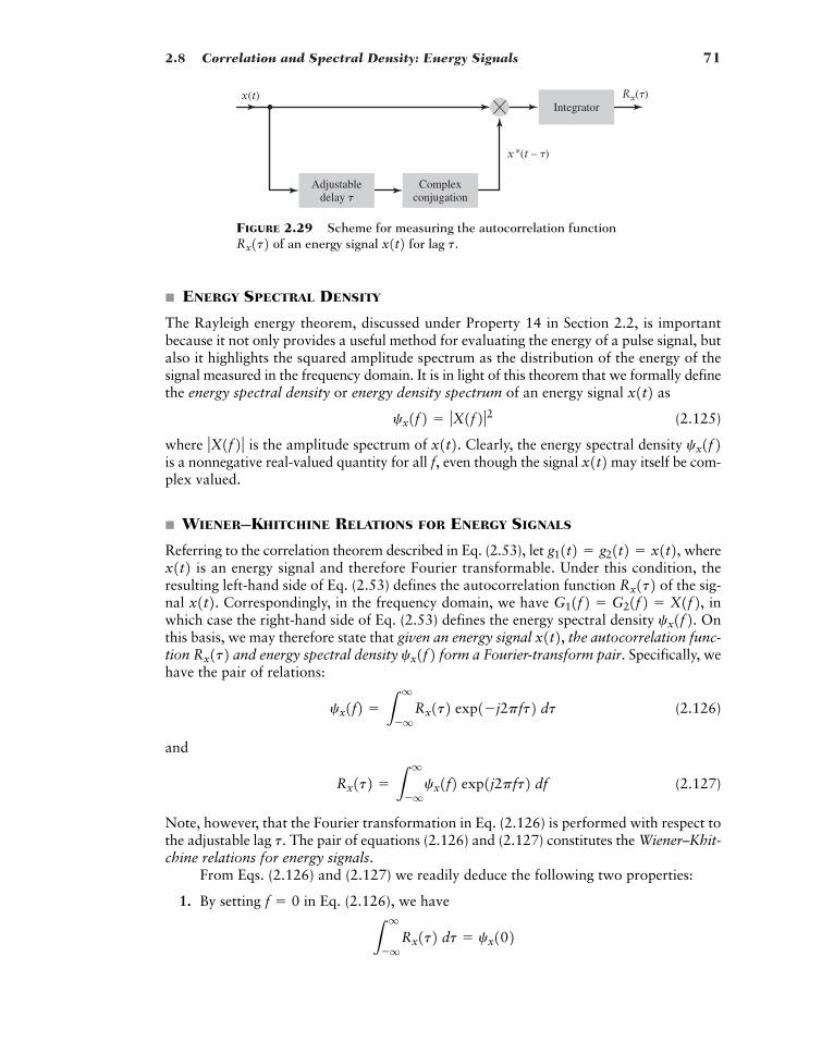
2.8 Correlation and Spectral Density: Energy Signals 71
x(t)Integrator
Adjustabledelay �
Complexconjugation
Rx(�)
x*(t – �)
FIGURE 2.29 Scheme for measuring the autocorrelation functionof an energy signal for lag .tx1t2Rx1t2
� ENERGY SPECTRAL DENSITY
The Rayleigh energy theorem, discussed under Property 14 in Section 2.2, is importantbecause it not only provides a useful method for evaluating the energy of a pulse signal, butalso it highlights the squared amplitude spectrum as the distribution of the energy of thesignal measured in the frequency domain. It is in light of this theorem that we formally definethe energy spectral density or energy density spectrum of an energy signal as
(2.125)
where is the amplitude spectrum of . Clearly, the energy spectral density is a nonnegative real-valued quantity for all even though the signal may itself be com-plex valued.
� WIENER–KHITCHINE RELATIONS FOR ENERGY SIGNALS
Referring to the correlation theorem described in Eq. (2.53), let whereis an energy signal and therefore Fourier transformable. Under this condition, the
resulting left-hand side of Eq. (2.53) defines the autocorrelation function of the sig-nal . Correspondingly, in the frequency domain, we have inwhich case the right-hand side of Eq. (2.53) defines the energy spectral density Onthis basis, we may therefore state that given an energy signal , the autocorrelation func-tion and energy spectral density form a Fourier-transform pair. Specifically, wehave the pair of relations:
(2.126)
and
(2.127)
Note, however, that the Fourier transformation in Eq. (2.126) is performed with respect tothe adjustable lag The pair of equations (2.126) and (2.127) constitutes the Wiener–Khit-chine relations for energy signals.
From Eqs. (2.126) and (2.127) we readily deduce the following two properties:
1. By setting in Eq. (2.126), we have
Lq
�qRx1t2 dt � cx102
f � 0
t.
Rx1t2 � Lq
�qcx1f2 exp1j2pft2 df
cx1f2 � Lq
�qRx1t2 exp1�j2pft2 dt
cx1f2Rx1t2 x1t2 cx1f2.G11f2 � G21f2 � X1f2,x1t2 Rx1t2x1t2 g11t2 � g21t2 � x1t2,
x1t2f,cx1f2x1t2ƒX1f2 ƒ
cx1f2 � ƒX1f2 ƒ2x1t2
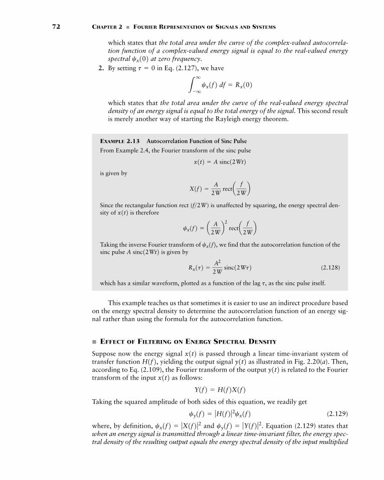
72 CHAPTER 2 � FOURIER REPRESENTATION OF SIGNALS AND SYSTEMS
which states that the total area under the curve of the complex-valued autocorrela-tion function of a complex-valued energy signal is equal to the real-valued energyspectral at zero frequency.
2. By setting in Eq. (2.127), we have
which states that the total area under the curve of the real-valued energy spectraldensity of an energy signal is equal to the total energy of the signal. This second resultis merely another way of starting the Rayleigh energy theorem.
EXAMPLE 2.13 Autocorrelation Function of Sinc Pulse
From Example 2.4, the Fourier transform of the sinc pulse
is given by
Since the rectangular function rect ( ) is unaffected by squaring, the energy spectral den-sity of is therefore
Taking the inverse Fourier transform of we find that the autocorrelation function of thesinc pulse is given by
(2.128)
which has a similar waveform, plotted as a function of the lag as the sinc pulse itself.
This example teaches us that sometimes it is easier to use an indirect procedure basedon the energy spectral density to determine the autocorrelation function of an energy sig-nal rather than using the formula for the autocorrelation function.
� EFFECT OF FILTERING ON ENERGY SPECTRAL DENSITY
Suppose now the energy signal is passed through a linear time-invariant system oftransfer function yielding the output signal as illustrated in Fig. 2.20(a). Then,according to Eq. (2.109), the Fourier transform of the output is related to the Fouriertransform of the input as follows:
Taking the squared amplitude of both sides of this equation, we readily get
(2.129)
where, by definition, and Equation (2.129) states thatwhen an energy signal is transmitted through a linear time-invariant filter, the energy spec-tral density of the resulting output equals the energy spectral density of the input multiplied
cy1f2 � ƒY1f2 ƒ2.cx1f2 � ƒX1f2 ƒ2cy1f2 � ƒH1f2 ƒ2cx1f2
Y1f2 � H1f2X1f2x1t2 y1t2y1t2H1f2, x1t2
t,
Rx1t2 �A2
2W sinc12Wt2
A sinc12Wt2 cx1f2,cx1f2 � a A
2Wb2
recta f
2Wb
x1t2 f>2W
X1f2 �A
2W recta f
2Wb
x1t2 � A sinc12Wt2
Lq
�qcx1f2 df � Rx102
t � 0cx102
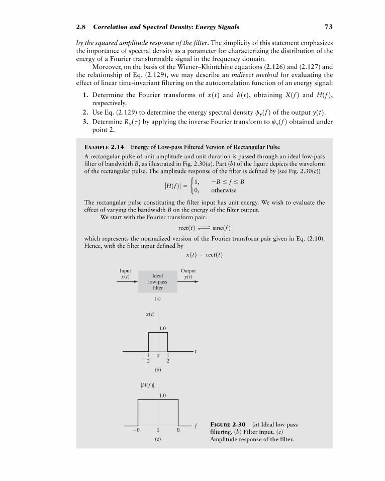
2.8 Correlation and Spectral Density: Energy Signals 73
Inputx(t)
Outputy(t)Ideal
low-passfilter
(a)
(b)
0
1.0
t
x(t)
– —12
—12
(c)
0
1.0
f
|H(f )|
–B BFIGURE 2.30 (a) Ideal low-passfiltering. (b) Filter input. (c)Amplitude response of the filter.
by the squared amplitude response of the filter. The simplicity of this statement emphasizesthe importance of spectral density as a parameter for characterizing the distribution of theenergy of a Fourier transformable signal in the frequency domain.
Moreover, on the basis of the Wiener–Khintchine equations (2.126) and (2.127) andthe relationship of Eq. (2.129), we may describe an indirect method for evaluating theeffect of linear time-invariant filtering on the autocorrelation function of an energy signal:
1. Determine the Fourier transforms of and , obtaining and respectively.
2. Use Eq. (2.129) to determine the energy spectral density of the output .3. Determine by applying the inverse Fourier transform to obtained under
point 2.
EXAMPLE 2.14 Energy of Low-pass Filtered Version of Rectangular Pulse
A rectangular pulse of unit amplitude and unit duration is passed through an ideal low-passfilter of bandwidth B, as illustrated in Fig. 2.30(a). Part (b) of the figure depicts the waveformof the rectangular pulse. The amplitude response of the filter is defined by (see Fig. 2.30(c))
The rectangular pulse constituting the filter input has unit energy. We wish to evaluate theeffect of varying the bandwidth B on the energy of the filter output.
We start with the Fourier transform pair:
which represents the normalized version of the Fourier-transform pair given in Eq. (2.10).Hence, with the filter input defined by
x1t2 � rect1t2
rect1t2 Δ sinc1f2
ƒH1f2 ƒ � b1, �B � f � B0, otherwise
cy1f2Ry1t2y1t2cy1f2
H1f2,X1f2h1t2x1t2
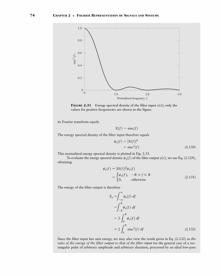
74 CHAPTER 2 � FOURIER REPRESENTATION OF SIGNALS AND SYSTEMS
Normalized frequency, f1.00
02.0 3.0
0.2
0.4
0.6
0.8
1.0
sinc
2 (f )
FIGURE 2.31 Energy spectral density of the filter input only thevalues for positive frequencies are shown in the figure.
x1t2;
its Fourier transform equals
The energy spectral density of the filter input therefore equals
(2.130)
This normalized energy spectral density is plotted in Fig. 2.31.To evaluate the energy spectral density of the filter output , we use Eq. (2.129),
obtaining
(2.131)
The energy of the filter output is therefore
(2.132)
Since the filter input has unit energy, we may also view the result given in Eq. (2.132) as theratio of the energy of the filter output to that of the filter input for the general case of a rec-tangular pulse of arbitrary amplitude and arbitrary duration, processed by an ideal low-pass
� 2LB
0 sinc21f2 df
� 2LB
0cx1f2 df
�LB
�Bcx1f2 df
Ey �Lq
�qcy1f2 df
� bcx1f2, �B � f � B0, otherwise
cy1f2 � ƒH1f2 ƒ2cx1f2y1t2cy1f2
� sinc21f2cx1f2 � ƒX1f2 ƒ2X1f2 � sinc1f2
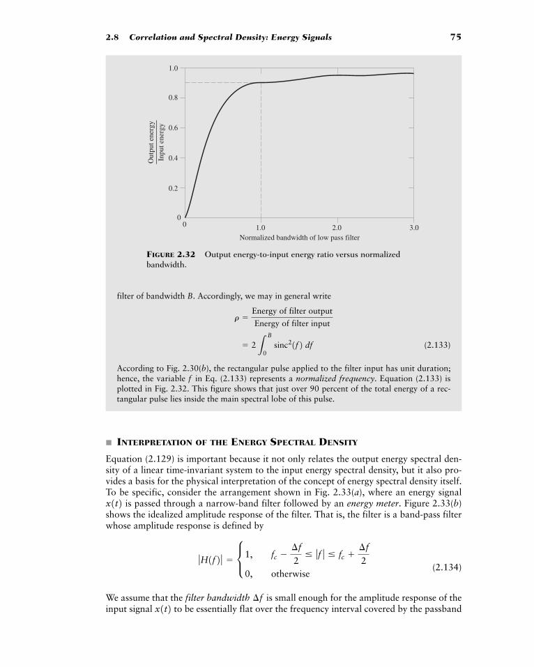
2.8 Correlation and Spectral Density: Energy Signals 75
Normalized bandwidth of low pass filter1.00
02.0 3.0
0.2
0.4
0.6
0.8
1.0
Out
put e
nerg
yIn
put e
nerg
y
filter of bandwidth B. Accordingly, we may in general write
(2.133)
According to Fig. 2.30(b), the rectangular pulse applied to the filter input has unit duration;hence, the variable in Eq. (2.133) represents a normalized frequency. Equation (2.133) isplotted in Fig. 2.32. This figure shows that just over 90 percent of the total energy of a rec-tangular pulse lies inside the main spectral lobe of this pulse.
� INTERPRETATION OF THE ENERGY SPECTRAL DENSITY
Equation (2.129) is important because it not only relates the output energy spectral den-sity of a linear time-invariant system to the input energy spectral density, but it also pro-vides a basis for the physical interpretation of the concept of energy spectral density itself.To be specific, consider the arrangement shown in Fig. 2.33(a), where an energy signal
is passed through a narrow-band filter followed by an energy meter. Figure 2.33(b)shows the idealized amplitude response of the filter. That is, the filter is a band-pass filterwhose amplitude response is defined by
(2.134)
We assume that the filter bandwidth is small enough for the amplitude response of theinput signal to be essentially flat over the frequency interval covered by the passbandx1t2 ¢f
ƒH1f2 ƒ � c 1, fc �¢f
2� ƒf ƒ � fc
¢f
20, otherwise
x1t2
f
� 2LB
0 sinc21f2 df
r �Energy of filter output
Energy of filter input
FIGURE 2.32 Output energy-to-input energy ratio versus normalizedbandwidth.
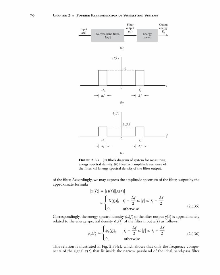
76 CHAPTER 2 � FOURIER REPRESENTATION OF SIGNALS AND SYSTEMS
Inputx(t)
Outputenergy
Ey
Filteroutputy(t)
Narrow-band filter,H(f )
Energymeter
(a)
(b)
0
1.0
f
|H(f )|
–fc fc
�f�f
(c)
0f
�y(f )
�x(fc)
–fc fc
�f�f
FIGURE 2.33 (a) Block diagram of system for measuringenergy spectral density. (b) Idealized amplitude response ofthe filter. (c) Energy spectral density of the filter output.
of the filter. Accordingly, we may express the amplitude spectrum of the filter output by theapproximate formula
(2.135)
Correspondingly, the energy spectral density of the filter output is approximatelyrelated to the energy spectral density of the filter input as follows:
(2.136)
This relation is illustrated in Fig. 2.33(c), which shows that only the frequency compo-nents of the signal that lie inside the narrow passband of the ideal band-pass filterx1t2
cy1f2 � c cx1fc2, fc �¢f
2� ƒf ƒ � fc
¢f
20, otherwise
x1t2cx1f2 y1t2cy1f2� c ƒX1fc2 ƒ , fc �
¢f
2� ƒf ƒ � fc
¢f
20, otherwise
ƒY1f2 ƒ � ƒH1f2 ƒ ƒX1f2 ƒ
2.8 Correlation and Spectral Density: Energy Signals 77
reach the output. From Rayleigh’s energy theorem, the energy of the filter output isgiven by
In light of Eq. (2.136), we may approximate as
(2.137)
The multiplying factor 2 accounts for the contributions of negative as well as positive fre-quency components. We may rewrite Eq. (2.137) in the form
(2.138)
Equation (2.138) states that the energy spectral density of the filter input at some frequencyequals the energy of the filter output divided by where is the filter bandwidth
centered on We may therefore interpret the energy spectral density of an energy signalfor any frequency f as the energy per unit bandwidth, which is contributed by frequencycomponents of the signal around the frequency f.
The arrangement shown in the block diagram of Fig. 2.33(a) thus provides the basisfor measuring the energy spectral density of an energy signal. Specifically, by using a vari-able band-pass filter to scan the frequency band of interest and determining the energy ofthe filter output for each midband frequency setting of the filter, a plot of the energy spec-tral density versus frequency is obtained. Note, however, for the formula of Eq. (2.138) tohold and therefore for the arrangement of Fig. 2.33(a) to work, the bandwidth mustremain fixed for varying
� CROSS-CORRELATION OF ENERGY SIGNALS
The autocorrelation function provides a measure of the similarity between a signal and itsown time-delayed version. In a similar way, we may use the cross-correlation function asa measure of the similarity between one signal and the time-delayed version of a second sig-nal. Let and denote a pair of complex-valued energy signals. The cross-correlationfunction of this pair of signals is defined by
(2.139)
We see that if the two signals and are somewhat similar, then the cross-correla-tion function will be finite over some range of thereby providing a quantitativemeasure of the similarity, or coherence, between them. The energy signals and aresaid to be orthogonal over the entire time interval if is zero — that is, if
(2.140)
Equation (2.139) defines one possible value for the cross-correlation function for a speci-fied value of the delay variable We may define a second cross-correlation function fort.
Lq
�qx1t2y*1t2 dt � 0
Rxy102 y1t2x1t2t,Rxy1t2 y1t2x1t2Rxy1t2 �L
q
�qx1t2y*1t � t2 dt
y1t2x1t2
fc .¢f
fc .¢f2¢f,fc
cx1fc2 �Ey
2¢f
Ey � 2cx1fc2 ¢f
Ey
� 2Lq
0cy1f2 df
Ey �Lq
�qcy1f2 df
y1t2
78 CHAPTER 2 � FOURIER REPRESENTATION OF SIGNALS AND SYSTEMS
the energy signals and as
(2.141)
From the definitions of the cross-correlation functions and just given, weobtain the fundamental relationship
(2.142)
Equation (2.142) indicates that unlike convolution, correlation is not in general commu-tative; that is,
To characterize the cross-correlation behavior of energy signals in the frequencydomain, we introduce the notion of cross-spectral density. Specifically, given a pair of com-plex-valued energy signals and , we define their cross-spectral densities, denotedby and as the respective Fourier transforms of the cross-correlation functions
and as shown by
(2.143)
and
(2.144)
In accordance with the correlation theorem (i.e., Property 13 of Section 2.2), we thus have
(2.145)
and
(2.146)
From this pair of relations, we readily see two properties of the cross-spectral density.
1. Unlike the energy spectral density, cross-spectral density is complex valued in general.2. from which it follows that, in general,
� Drill Problem 2.15 Derive the relationship of Eq. (2.142) between the two cross-correlation functions and �
� Drill Problem 2.16 Consider the decaying exponential pulse
Determine the energy spectral density of the pulse �
� Drill Problem 2.17 Repeat Problem 2.16 for the double exponential pulse
�g1t2 � c exp1�at2, t � 01, t � 0exp1at2, t � 0
g1t2.g1t2 � c exp1�at2, t � 0
1, t � 00, t � 0
Ryx1t2.Rxy1t2
cxy1f2 cyx1f2.cxy1f2 � cyx… 1f2
cyx1f2 � Y1f2X*1f2cxy1f2 � X1f2Y*1f2
cyx1f2 � Lq
�qRyx1t2 exp1�j2pft2 dt
cxy1f2 �Lq
�qRxy1t2 exp1�j2pft2 dt
Ryx1t2,Rxy1t2 cyx1f2,cxy1f2 y1t2x1t2Rxy1t2 Ryx1t2.
Rxy1t2 � Ryx… 1�t2
Ryx1t2Rxy1t2Ryx1t2 �L
q
�qy1t2x*1t � t2 dt
y1t2x1t2
2.9 Power Spectral Density 79
2.9 Power Spectral Density
In this section, we expand the important notion of spectral density to include the class ofpower signals. The average power of a signal is defined by
(2.147)
The signal is said to be a power signal if the condition
holds. Examples of power signals include periodic signals and noise. We consider periodicsignals in this section. (Noise is considered in Chapter 8.)
To develop a frequency-domain distribution of power, we need to know the Fouriertransform of the signal However, this may pose a problem, because power signalshave infinite energy and may therefore not be Fourier transformable. To overcome theproblem, we consider a truncated version of the signal In particular, we define
(2.148)
As long as the duration T is finite, the truncated signal has finite energy; hence is Fourier transformable. Let denote the Fourier transform of that is,
Using the truncated signal we may rewrite Eq. (2.147) for the average power P interms of as
(2.149)
Since has finite energy, we may use the Rayleigh energy theorem to express the energyof in terms of its Fourier transform as
where is the amplitude spectrum of Accordingly, we may rewrite Eq. (2.149)in the equivalent form
(2.150)
As the duration T increases, the energy of increases. Correspondingly, the energyspectral density increases with T. Indeed as T approaches infinity, so will
However, for the average power P to be finite, must approach infinity at the same rate as T. This requirement ensures the convergence of the integral on the right-hand side of Eq. (2.150) in the limit as T approaches infinity. The convergence, in turn, per-mits us to interchange the order in which the limiting operation and integration inEq. (2.150) are performed. We may then rewrite this equation as
(2.151)P � Lq
�qa lim
TS�
12T
ƒXT1f2 ƒ2b df
ƒXT1f2 ƒ2ƒXT1f2 ƒ2.ƒXT1f2 ƒ2 xT1t2
P � limTS�
12T L
q
�qƒXT1f2 ƒ2 df
xT1t2.ƒXT1f2 ƒL
q
�qƒxT1t2 ƒ2 dt � L
q
�qƒXT1f2 ƒ2 df
XT1f2xT1t2xT1t2P � lim
TS�
12T L
q
�qƒxT1t2 ƒ2 dt
xT1t2 xT1t2,xT1t2 Δ XT1f2
xT1t2;XT1f2 xT1t2xT1t2� bx1t2, �T � t � T
0, otherwise
xT1t2 � x1t2 recta t2Tb
x1t2.x1t2.
P � �
x1t2P � lim
TS�
12T L
T
�Tƒx1t2 ƒ2 dt
x1t2
80 CHAPTER 2 � FOURIER REPRESENTATION OF SIGNALS AND SYSTEMS
Let the integrand in Eq. (2.151) be denoted by
(2.152)
The frequency-dependent function is called the power spectral density or power spec-trum of the power signal , and the quantity is called the periodogram ofthe signal.
From Eq. (2.152), we readily see that the power spectral density is a nonnegativereal-valued quantity for all frequencies. Moreover, from Eq. (2.152) we readily see that
(2.153)
Equation (2.153) states: the total area under the curve of the power spectral density of apower signal is equal to the average power of that signal. The power spectral density of apower signal therefore plays a role similar to the energy spectral density of an energy signal.
� Drill Problem 2.18 In an implicit sense, Eq. (2.153) embodies Parseval’s power theo-rem, which states that for a periodic signal x(t) we have
where T is the period of the signal, is the fundamental frequency, and is the Fouriertransform of evaluated at the frequency Prove this theorem. �
EXAMPLE 2.15 Modulated Wave
Consider the modulated wave
(2.154)
where is a power signal that is band-limited to B hertz. We refer to as a “modulatedwave” in the sense that the amplitude of the sinusoidal “carrier” of frequency is varied lin-early with the signal (The subject of modulation is covered in detail in Chapter 3.) Wewish to find the power spectral density of in terms of that of given that the frequency
is larger than the bandwidth B.Let denote the truncated version of defined in a manner similar to that
described in Eq. (2.148). Correspondingly, we may express the truncated version of as
(2.155)
Since
(2.156)
it follows from the frequency-shifting property (i. e., Property 6) of the Fourier transform that
(2.157)
where is the Fourier transform of gT1t2.GT1f2XT1f2 �
123GT1f � fc2 GT1f fc24
cos12pfct2 �123exp1j2pfct2 exp1�j2pfct24,
xT1t2 � gT1t2 cos12pfct2x1t2g1t2,gT1t2fc
g1t2,x1t2g1t2. fcx1t2g1t2
x1t2 � g1t2 cos12pfct2
nf0 .x1t2 X1nf02f0
1T L
T>2�T>2 ƒx1t2 ƒ2 dt � a
q
n� ��ƒX1nf02 ƒ2
P � Lq
�qSx1f2 df
1 ƒXT1f2 ƒ2>2T2x1t2 Sx1f2Sx1f2 � lim
TS�
12T
ƒXT1f2 ƒ2
2.10 Numerical Computation of the Fourier Transform 81
Given that we find that and represent nonoverlappingspectra; their product is therefore zero. Accordingly, using Eq. (2.157) to evaluate the squaredamplitude of we get
(2.158)
Finally, applying the definition of Eq. (2.152) for the power spectral density of the power sig-nal to Eq (2.158), we get the desired result:
(2.159)
Except for the scaling factor the power spectral density of the modulated wave is equalto the sum of the power spectral density shifted to the right by and the shifted tothe left by the same amount
2.10 Numerical Computation of the Fourier Transform
The material presented in this chapter clearly testifies to the importance of the Fouriertransform as a theoretical tool for the representation of deterministic signals and lineartime-invariant systems. The importance of the Fourier transform is further enhanced by thefact that there exists a class of algorithms called fast Fourier transform algorithms for thenumerical computation of the Fourier transform in a highly efficient manner.
The fast Fourier transform algorithm is itself derived from the discrete Fourier trans-form in which, as the name implies, both time and frequency are represented in discreteform. The discrete Fourier transform provides an approximation to the Fourier transform.In order to properly represent the information content of the original signal, we have to takespecial care in performing the sampling operations involved in defining the discrete Fouriertransform. A detailed treatment of the sampling process will be presented in Chapter 5. Forthe present, it suffices to say that given a band-limited signal, the sampling rate should begreater than twice the highest frequency component of the input signal. Moreover, if thesamples are uniformly spaced by seconds, the spectrum of the signal becomes periodic,repeating every Hz. Let N denote the number of frequency samples containedin an interval Hence, the frequency resolution involved in the numerical computationof the Fourier transform is defined by
(2.160)
where is the total duration of the signal.Consider then a finite data sequence For brevity, we refer to this
sequence as in which the subscript is the time index Such asequence may represent the result of sampling an analog signal at times
where is the sampling interval. The ordering of the datasequence defines the sample time in that denote samples of taken attimes 0, respectively. Thus we have
(2.161)gn � g1nTs2Ts , Á , 1N � 12Ts ,
g1t2g0, g1, Á , gN�1
Tst � 0, Ts , Á , 1N � 12Ts ,g1t2n � 0, 1, Á , N � 1.gn ,
5g0, g1, Á , gN�16.T � NTs
¢f �fsN
�1
NTs�
1T
fs .fs � 11>Ts2 Ts
fc .Sg1f2fcSg1f2 x1t21>4,
Sx1f2 �143Sg1f � fc2 Sg1f fc24
g1t2ƒXT1f2 ƒ2 �
143 ƒGT1f � fc2 ƒ2 ƒGT1f fc2 ƒ24
XT1f2,GT1f fc2GT1f � fc2fc � B,
82 CHAPTER 2 � FOURIER REPRESENTATION OF SIGNALS AND SYSTEMS
We formally define the discrete Fourier transform (DFT) of the sequence as
(2.162)
The sequence is called the transform sequence. For brevity, we referto this new sequence as in which the subscript is the frequency index
Correspondingly, we define the inverse discrete Fourier transform(IDFT) of as
(2.163)
The DFT and the IDFT form a transform pair. Specifically, given the data sequence wemay use the DFT to compute the transform sequence and given the transform sequence
we may use the IDFT to recover the original data sequence A distinctive feature ofthe DFT is that for the finite summations defined in Eqs. (2.162) and (2.163), there is noquestion of convergence.
When discussing the DFT (and algorithms for its computation), the words “sample”and “point” are used interchangeably to refer to a sequence value. Also, it is common prac-tice to refer to a sequence of length N as an N-point sequence, and refer to the DFT of adata sequence of length N as an N-point DFT.
� INTERPRETATIONS OF THE DFT AND THE IDFT
We may visualize the DFT process, described in Eq. (2.162), as a collection of N complexheterodyning and averaging operations, as shown in Fig. 2.34(a); in the picture depictedherein, heterodyning refers to the multiplication of data sequence by a complex expo-nential. We say that the heterodyning is complex in that samples of the data sequence aremultiplied by complex exponential sequences. There are a total of N complex exponentialsequences to be considered, corresponding to the frequency index Their periods have been selected in such a way that each complex exponential sequence hasprecisely an integer number of cycles in the total interval 0 to The zero-frequencyresponse, corresponding to is the only exception.
For the interpretation of the IDFT process, described in Eq. (2.163), we may use thescheme shown in Fig. 2.34(b). Here we have a collection of N complex signal generators,each of which produces the complex exponential sequence
(2.164)
Thus, in reality, each complex signal generator consists of a pair of generators that outputa cosinusoidal and a sinusoidal sequence of k cycles per observation interval. The outputof each complex signal generator is weighted by the complex Fourier coefficient At eachtime index n, an output is formed by summing the weighted complex generator outputs.
It is noteworthy that although the DFT and the IDFT are similar in their mathemat-ical formulations, as described in Eqs. (2.162) and (2.163), their interpretations, as depictedin Figs. 2.34(a) and 2.34(b), are so completely different.
Also, the addition of harmonically related periodic signals, as in Figs. 2.34(a) and2.34(b), suggests that the sequences and must be both periodic. Moreover, the proces-gnGk
Gk .
� ecosa2pN
knb, sina2pN
knb f, k � 0, 1, Á , N � 1
expa j2p
Nknb � cosa2p
Nknb j sina2p
Nknb
k � 0,N � 1.
k � 0, 1, Á , N � 1.
gn
gn .Gk ,Gk ;
gn ,
gn �1N a
N�1
k�0Gk expa j2p
Nknb , n � 0, 1, Á , N � 1
Gk
k � 0, 1, Á , N � 1.Gk ,
5G0, G1, Á , GN�16Gk � a
N�1
n�0gn expa�
j2p
Nknb , k � 0, 1, Á , N � 1
gn
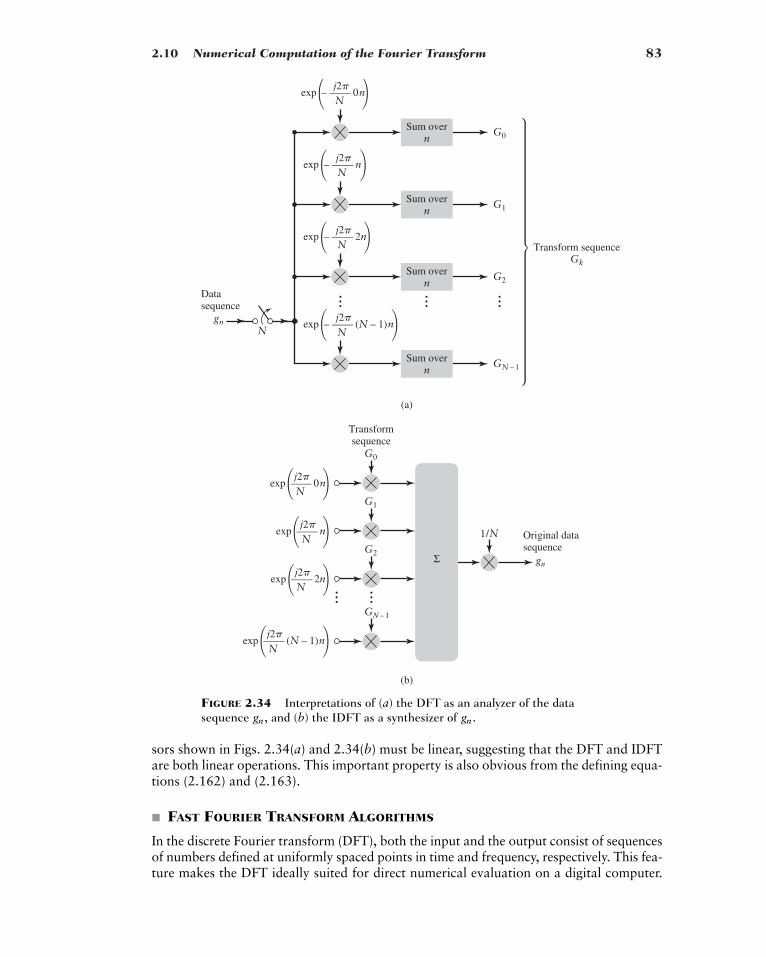
2.10 Numerical Computation of the Fourier Transform 83
(a)
(b)
Sum overn
G0
Sum overn
G1
Sum overn
G2
Sum overn
Datasequence
Transform sequenceGk
GN – 1
gnN
exp (N – 1)nj2�
– ——q rN
exp 2nj2�
– ——q rN
exp nj2�
– ——q rN
... ... ...
1/N Original datasequence
gn
Transformsequence
exp (N – 1)nj2�
——q rN
exp 0n
G0
j2�——q rN
exp n
G1
j2�——q rN
exp 2n
G2
j2�——q rN
GN – 1
... ...
Σ
exp 0nj2�
– ——q rN
FIGURE 2.34 Interpretations of (a) the DFT as an analyzer of the datasequence and (b) the IDFT as a synthesizer of gn .gn ,
sors shown in Figs. 2.34(a) and 2.34(b) must be linear, suggesting that the DFT and IDFTare both linear operations. This important property is also obvious from the defining equa-tions (2.162) and (2.163).
� FAST FOURIER TRANSFORM ALGORITHMS
In the discrete Fourier transform (DFT), both the input and the output consist of sequencesof numbers defined at uniformly spaced points in time and frequency, respectively. This fea-ture makes the DFT ideally suited for direct numerical evaluation on a digital computer.
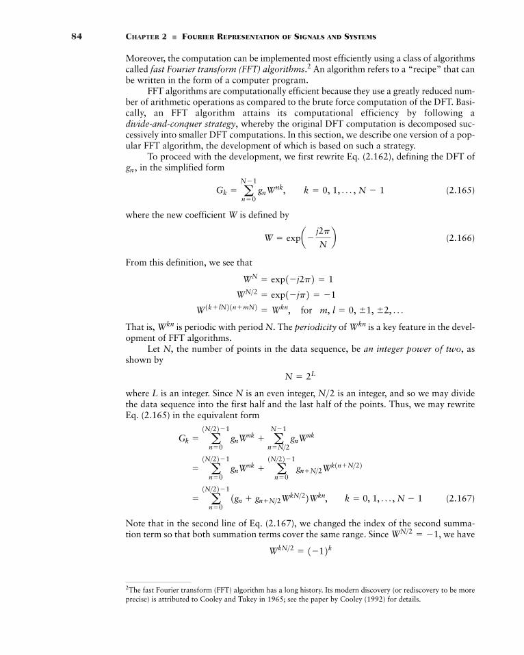
84 CHAPTER 2 � FOURIER REPRESENTATION OF SIGNALS AND SYSTEMS
Moreover, the computation can be implemented most efficiently using a class of algorithmscalled fast Fourier transform (FFT) algorithms.2 An algorithm refers to a “recipe” that canbe written in the form of a computer program.
FFT algorithms are computationally efficient because they use a greatly reduced num-ber of arithmetic operations as compared to the brute force computation of the DFT. Basi-cally, an FFT algorithm attains its computational efficiency by following adivide-and-conquer strategy, whereby the original DFT computation is decomposed suc-cessively into smaller DFT computations. In this section, we describe one version of a pop-ular FFT algorithm, the development of which is based on such a strategy.
To proceed with the development, we first rewrite Eq. (2.162), defining the DFT ofin the simplified form
(2.165)
where the new coefficient W is defined by
(2.166)
From this definition, we see that
That is, is periodic with period N. The periodicity of is a key feature in the devel-opment of FFT algorithms.
Let N, the number of points in the data sequence, be an integer power of two, asshown by
where L is an integer. Since N is an even integer, is an integer, and so we may dividethe data sequence into the first half and the last half of the points. Thus, we may rewriteEq. (2.165) in the equivalent form
(2.167)
Note that in the second line of Eq. (2.167), we changed the index of the second summa-tion term so that both summation terms cover the same range. Since we have
WkN>2 � 1�12kWN>2 � �1,
� a1N>22�1
n�01gn gnN>2WkN>22Wkn, k � 0, 1, Á , N � 1
� a1N>22�1
n�0gnWnk a
1N>22�1
n�0gnN>2Wk1nN>22
Gk � a1N>22�1
n�0gnWnk a
N�1
n�N>2gnWnk
N>2N � 2L
WknWkn
W1k lN21nmN2 � Wkn, for m, l � 0, �1, �2, Á
WN>2 � exp1�jp2 � �1
WN � exp1�j2p2 � 1
W � expa�j2p
Nb
Gk � aN�1
n�0gnWnk, k � 0, 1, Á , N � 1
gn ,
2The fast Fourier transform (FFT) algorithm has a long history. Its modern discovery (or rediscovery to be moreprecise) is attributed to Cooley and Tukey in 1965; see the paper by Cooley (1992) for details.
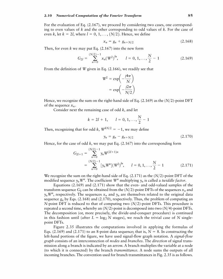
2.10 Numerical Computation of the Fourier Transform 85
For the evaluation of Eq. (2.167), we proceed by considering two cases, one correspond-ing to even values of k and the other corresponding to odd values of k. For the case ofeven k, let where Hence, we define
(2.168)
Then, for even k we may put Eq. (2.167) into the new form
(2.169)
From the definition of W given in Eq. (2.166), we readily see that
Hence, we recognize the sum on the right-hand side of Eq. (2.169) as the ( )-point DFTof the sequence
Consider next the remaining case of odd k, and let
Then, recognizing that for odd we may define
(2.170)
Hence, for the case of odd k, we may put Eq. (2.167) into the corresponding form
(2.171)
We recognize the sum on the right-hand side of Eq. (2.171) as the ( )-point DFT of themodified sequence The coefficient multiplying is called a twiddle factor.
Equations (2.169) and (2.171) show that the even- and odd-valued samples of thetransform sequence can be obtained from the ( )-point DFTs of the sequences and
respectively. The sequences and are themselves related to the original datasequence by Eqs. (2.168) and (2.170), respectively. Thus, the problem of computing anN-point DFT is reduced to that of computing two ( )-point DFTs. This procedure isrepeated a second time, whereby an ( )-point is decomposed into two ( )-point DFTs.The decomposition (or, more precisely, the divide-and-conquer procedure) is continuedin this fashion until (after stages), we reach the trivial case of N single-point DFTs.
Figure 2.35 illustrates the computations involved in applying the formulas ofEqs. (2.169) and (2.171) to an 8-point data sequence; that is, In constructing theleft-hand portions of the figure, we have used signal-flow graph notation. A signal-flowgraph consists of an interconnection of nodes and branches. The direction of signal trans-mission along a branch is indicated by an arrow. A branch multiplies the variable at a node(to which it is connected) by the branch transmittance. A node sums the outputs of allincoming branches. The convention used for branch transmittances in Fig. 2.35 is as follows.
N � 8.
L � log2 N
N>4N>2 N>2gn
ynxnynWn,xnN>2Gk
ynWnynWn.N>2
� a1N>22�1
n�03ynWn41W22ln, l � 0, 1, Á ,
N2
� 1
G2l1 � a1N>22�1
n�0ynW12l12n
yn � gn � gnN>2k, WkN>2 � �1,
k � 2l 1, l � 0, 1, Á ,N2
� 1
xn .N>2
� expa�j2p
N>2bW2 � expa�
j4p
Nb
G2l � a1N>22�1
n�0xn1W22ln, l � 0, 1, Á ,
N2
� 1
xn � gn gnN>2l � 0, 1, Á , 1N>22.k � 2l,
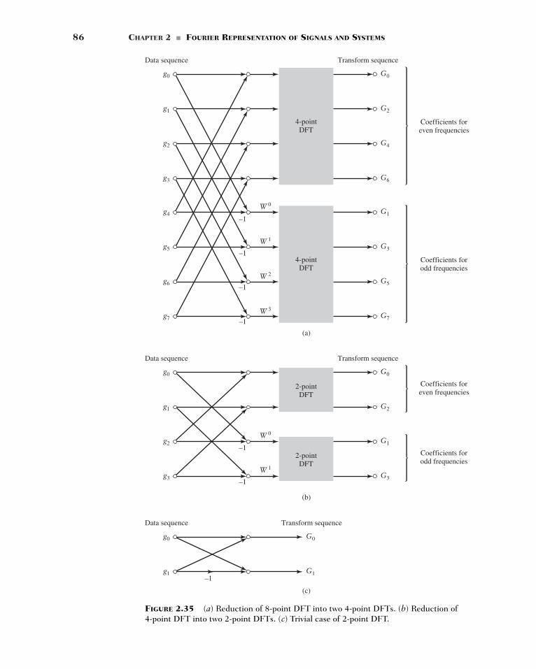
86 CHAPTER 2 � FOURIER REPRESENTATION OF SIGNALS AND SYSTEMS
g0 G0
Transform sequence
Coefficients foreven frequencies
Data sequence
4-pointDFT
g1 G2
g2 G4
g3 G6
g0 G0
Transform sequence
Coefficients foreven frequencies
Data sequence
2-pointDFT
g1 G2
g0 G0
Transform sequenceData sequence
g1 G1
g2 G1
Coefficients forodd frequencies
2-pointDFT
g3 G3
g4 G1W 0
–1
–1
–1
–1
–1
–1
–1
W 1
W 2
W 0
W 1
W 3
Coefficients forodd frequencies
4-pointDFT
(a)
(b)
(c)
g5 G3
g6 G5
g7 G7
FIGURE 2.35 (a) Reduction of 8-point DFT into two 4-point DFTs. (b) Reduction of4-point DFT into two 2-point DFTs. (c) Trivial case of 2-point DFT.
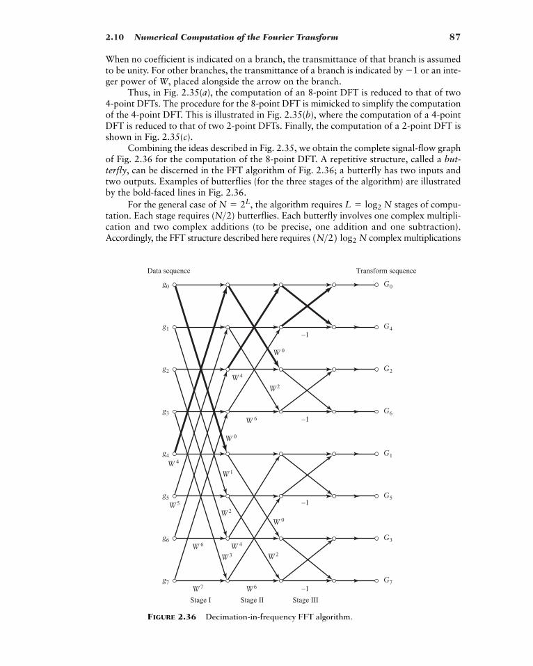
2.10 Numerical Computation of the Fourier Transform 87
When no coefficient is indicated on a branch, the transmittance of that branch is assumedto be unity. For other branches, the transmittance of a branch is indicated by or an inte-ger power of W, placed alongside the arrow on the branch.
Thus, in Fig. 2.35(a), the computation of an 8-point DFT is reduced to that of two4-point DFTs. The procedure for the 8-point DFT is mimicked to simplify the computationof the 4-point DFT. This is illustrated in Fig. 2.35(b), where the computation of a 4-pointDFT is reduced to that of two 2-point DFTs. Finally, the computation of a 2-point DFT isshown in Fig. 2.35(c).
Combining the ideas described in Fig. 2.35, we obtain the complete signal-flow graphof Fig. 2.36 for the computation of the 8-point DFT. A repetitive structure, called a but-terfly, can be discerned in the FFT algorithm of Fig. 2.36; a butterfly has two inputs andtwo outputs. Examples of butterflies (for the three stages of the algorithm) are illustratedby the bold-faced lines in Fig. 2.36.
For the general case of the algorithm requires stages of compu-tation. Each stage requires ( ) butterflies. Each butterfly involves one complex multipli-cation and two complex additions (to be precise, one addition and one subtraction).Accordingly, the FFT structure described here requires complex multiplications1N>22 log2 N
N>2 L � log2 NN � 2L,
�1
g0 G0
g1 G4
g2 G2
g3 G6
g4 G1
g5 G5
g6 G3
g7
Stage I Stage II Stage III
G7
Transform sequenceData sequence
W 0
W 0
W 0
W 1
W 5
W 2
W2
W 4
W 4
W 4W 6
W 3 W 2
W 7 W 6
W 6
–1
–1
–1
–1
FIGURE 2.36 Decimation-in-frequency FFT algorithm.
88 CHAPTER 2 � FOURIER REPRESENTATION OF SIGNALS AND SYSTEMS
and complex additions. (Actually, the number of multiplications quoted is pessimistic , because we may omit all twiddle factors and
) This computational complexity is significantly smaller than that of the com-plex multiplications and complex additions required for the direct computationof the DFT. The computational savings made possible by the FFT algorithm become moresubstantial as we increase the data length N.
We may establish two other important features of the FFT algorithm by carefullyexamining the signal-flow graph shown in Fig. 2.36:
1. At each stage of the computation, the new set of N complex numbers resulting fromthe computation can be stored in the same memory locations used to store the pre-vious set. This kind of computation is referred to as in-place computation.
2. The samples of the transform sequence are stored in a bit-reversed order. To illus-trate the meaning of this latter terminology, consider Table 2.2 constructed for the caseof At the left of the table, we show the eight possible values of the frequencyindex k (in their natural order) and their 3-bit binary representations. At the right ofthe table, we show the corresponding bit-reversed binary representations and indices.We observe that the bit-reversed indices in the right-most column of Table 2.2 appearin the same order as the indices at the output of the FFT algorithm in Fig. 2.36.
N � 8.
Gk
N1N � 12 N2W3N>4 � j.WN>4 � �j,WN>2 � �1,W0 � 1
N log2 N
TABLE 2.2 Illustrating Bit Reversal
Frequency Binary Bit-Reversed Bit-Reversed Index, k Representation Binary Representation Index
0 000 000 01 001 100 42 010 010 23 011 110 64 100 001 15 101 101 56 110 011 37 111 111 7
The FFT algorithm depicted in Fig. 2.36 is referred to as a decimation-in-frequency algorithm,because the transform (frequency) sequence is divided successively into smaller subse-quences. In another popular FFT algorithm, called a decimation-in-time algorithm, the data(time) sequence is divided successively into smaller subsequences. Both algorithms havethe same computational complexity. They differ from each other in two respects. First, fordecimation-in-frequency, the input is in natural order, whereas the output is in bit-reversedorder. The reverse is true for decimation-in-time. Second, the butterfly for decimation-in-timeis slightly different from that for decimation-in-frequency. The reader is invited to derivethe details of the decimation-in-time algorithm using the divide-and-conquer strategy thatled to the development of the algorithm described in Fig. 2.36; See Problem 2.50.
� COMPUTATION OF THE IDFT
The IDFT of the transform sequence is defined by Eq. (2.163). We may rewrite thisequation in terms of the complex parameter W as
(2.172)gn �1N a
N�1
k�0GkW�kn, n � 0, 1, Á , N � 1
Gk
gn
Gk
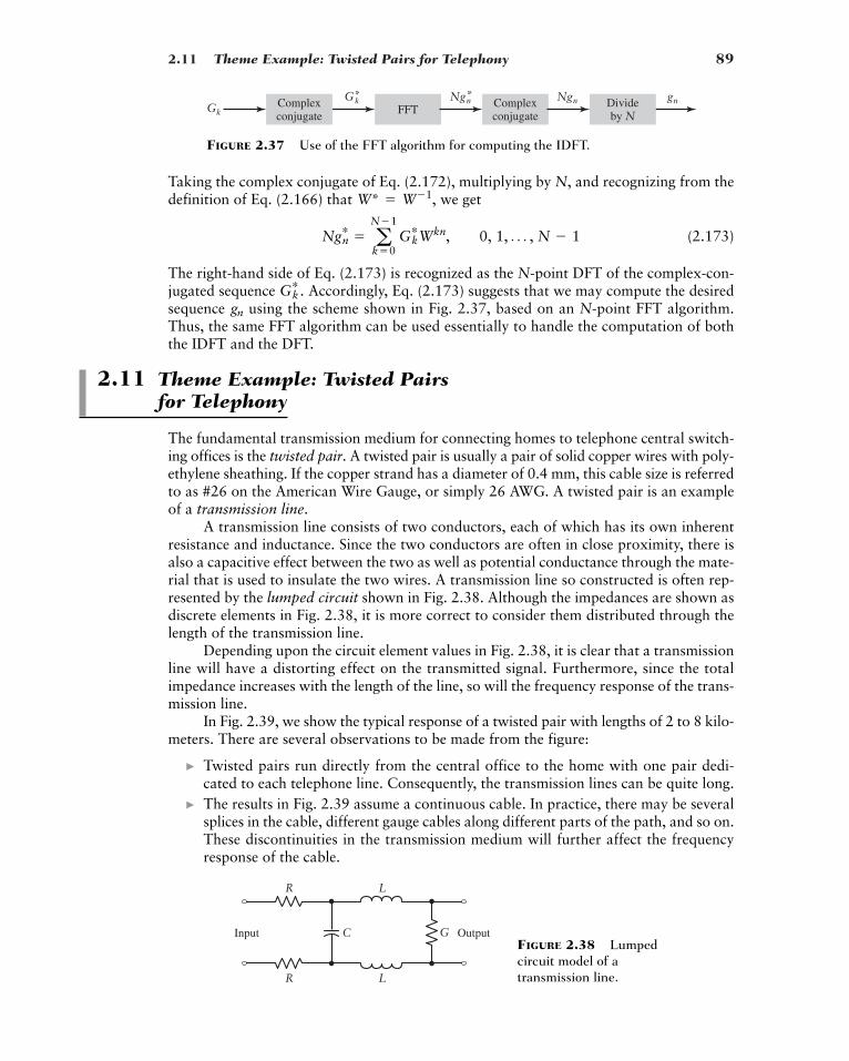
2.11 Theme Example: Twisted Pairs for Telephony 89
Complexconjugate
FFTComplexconjugate
Divideby N
Gk
G*k Ng*n Ngn gn
FIGURE 2.37 Use of the FFT algorithm for computing the IDFT.
GC OutputInput
LR
LR
FIGURE 2.38 Lumpedcircuit model of atransmission line.
Taking the complex conjugate of Eq. (2.172), multiplying by N, and recognizing from thedefinition of Eq. (2.166) that we get
(2.173)
The right-hand side of Eq. (2.173) is recognized as the N-point DFT of the complex-con-jugated sequence Accordingly, Eq. (2.173) suggests that we may compute the desiredsequence using the scheme shown in Fig. 2.37, based on an N-point FFT algorithm.Thus, the same FFT algorithm can be used essentially to handle the computation of boththe IDFT and the DFT.
2.11 Theme Example: Twisted Pairs for Telephony
The fundamental transmission medium for connecting homes to telephone central switch-ing offices is the twisted pair. A twisted pair is usually a pair of solid copper wires with poly-ethylene sheathing. If the copper strand has a diameter of 0.4 mm, this cable size is referredto as #26 on the American Wire Gauge, or simply 26 AWG. A twisted pair is an exampleof a transmission line.
A transmission line consists of two conductors, each of which has its own inherentresistance and inductance. Since the two conductors are often in close proximity, there isalso a capacitive effect between the two as well as potential conductance through the mate-rial that is used to insulate the two wires. A transmission line so constructed is often rep-resented by the lumped circuit shown in Fig. 2.38. Although the impedances are shown asdiscrete elements in Fig. 2.38, it is more correct to consider them distributed through thelength of the transmission line.
Depending upon the circuit element values in Fig. 2.38, it is clear that a transmissionline will have a distorting effect on the transmitted signal. Furthermore, since the totalimpedance increases with the length of the line, so will the frequency response of the trans-mission line.
In Fig. 2.39, we show the typical response of a twisted pair with lengths of 2 to 8 kilo-meters. There are several observations to be made from the figure:
� Twisted pairs run directly from the central office to the home with one pair dedi-cated to each telephone line. Consequently, the transmission lines can be quite long.
� The results in Fig. 2.39 assume a continuous cable. In practice, there may be severalsplices in the cable, different gauge cables along different parts of the path, and so on.These discontinuities in the transmission medium will further affect the frequencyresponse of the cable.
gn
Gk… .
Ngn… � a
N�1
k�0Gk…Wkn, 0, 1, Á , N � 1
W* � W�1,
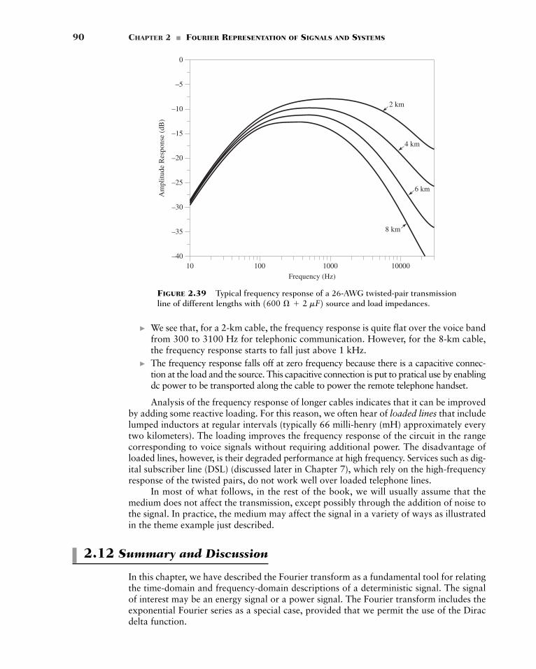
90 CHAPTER 2 � FOURIER REPRESENTATION OF SIGNALS AND SYSTEMS
10 100 1000 10000–40
–35
–30
–25
–20
–15
–10
–5
0
Am
plitu
de R
espo
nse
(dB
)
Frequency (Hz)
2 km
4 km
6 km
8 km
FIGURE 2.39 Typical frequency response of a 26-AWG twisted-pair transmissionline of different lengths with source and load impedances.1600 Æ 2 mF2
� We see that, for a 2-km cable, the frequency response is quite flat over the voice bandfrom 300 to 3100 Hz for telephonic communication. However, for the 8-km cable,the frequency response starts to fall just above 1 kHz.
� The frequency response falls off at zero frequency because there is a capacitive connec-tion at the load and the source. This capacitive connection is put to pratical use by enablingdc power to be transported along the cable to power the remote telephone handset.
Analysis of the frequency response of longer cables indicates that it can be improvedby adding some reactive loading. For this reason, we often hear of loaded lines that includelumped inductors at regular intervals (typically 66 milli-henry (mH) approximately everytwo kilometers). The loading improves the frequency response of the circuit in the rangecorresponding to voice signals without requiring additional power. The disadvantage ofloaded lines, however, is their degraded performance at high frequency. Services such as dig-ital subscriber line (DSL) (discussed later in Chapter 7), which rely on the high-frequencyresponse of the twisted pairs, do not work well over loaded telephone lines.
In most of what follows, in the rest of the book, we will usually assume that themedium does not affect the transmission, except possibly through the addition of noise tothe signal. In practice, the medium may affect the signal in a variety of ways as illustratedin the theme example just described.
2.12 Summary and Discussion
In this chapter, we have described the Fourier transform as a fundamental tool for relatingthe time-domain and frequency-domain descriptions of a deterministic signal. The signalof interest may be an energy signal or a power signal. The Fourier transform includes theexponential Fourier series as a special case, provided that we permit the use of the Diracdelta function.
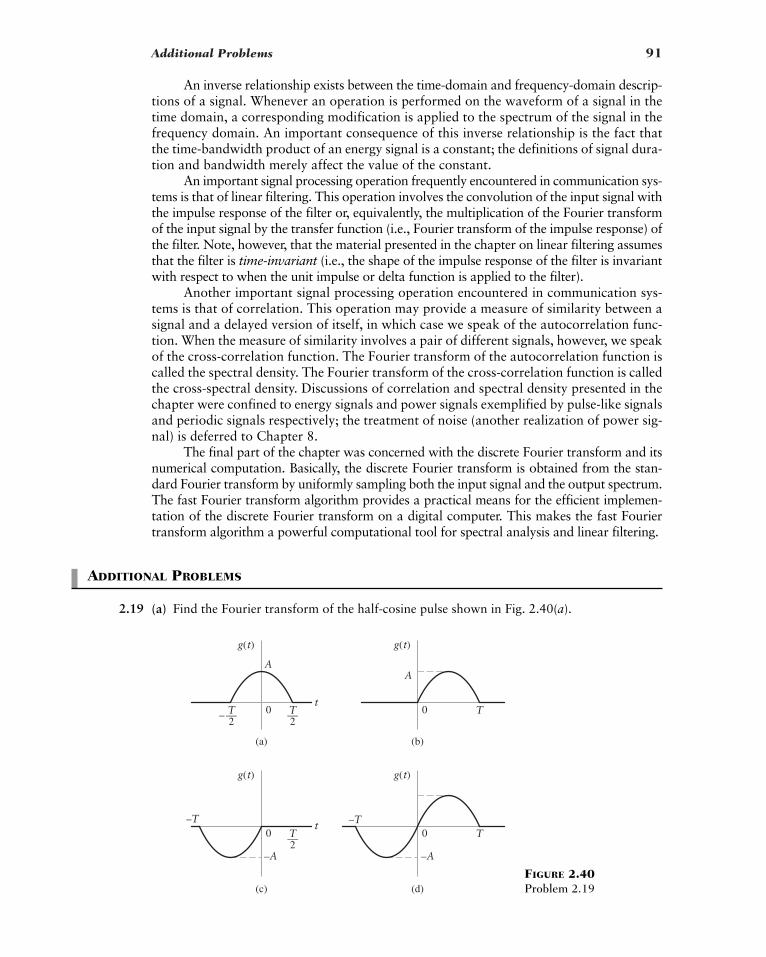
Additional Problems 91
(a) (b)
(c) (d)
0t
g(t)
–T
–A –A
–T
—T2
0
g(t)
T
0
A
t
g(t)
– —T2
—T2
0
A
g(t)
T
FIGURE 2.40Problem 2.19
An inverse relationship exists between the time-domain and frequency-domain descrip-tions of a signal. Whenever an operation is performed on the waveform of a signal in thetime domain, a corresponding modification is applied to the spectrum of the signal in thefrequency domain. An important consequence of this inverse relationship is the fact thatthe time-bandwidth product of an energy signal is a constant; the definitions of signal dura-tion and bandwidth merely affect the value of the constant.
An important signal processing operation frequently encountered in communication sys-tems is that of linear filtering. This operation involves the convolution of the input signal withthe impulse response of the filter or, equivalently, the multiplication of the Fourier transformof the input signal by the transfer function (i.e., Fourier transform of the impulse response) ofthe filter. Note, however, that the material presented in the chapter on linear filtering assumesthat the filter is time-invariant (i.e., the shape of the impulse response of the filter is invariantwith respect to when the unit impulse or delta function is applied to the filter).
Another important signal processing operation encountered in communication sys-tems is that of correlation. This operation may provide a measure of similarity between asignal and a delayed version of itself, in which case we speak of the autocorrelation func-tion. When the measure of similarity involves a pair of different signals, however, we speakof the cross-correlation function. The Fourier transform of the autocorrelation function iscalled the spectral density. The Fourier transform of the cross-correlation function is calledthe cross-spectral density. Discussions of correlation and spectral density presented in thechapter were confined to energy signals and power signals exemplified by pulse-like signalsand periodic signals respectively; the treatment of noise (another realization of power sig-nal) is deferred to Chapter 8.
The final part of the chapter was concerned with the discrete Fourier transform and itsnumerical computation. Basically, the discrete Fourier transform is obtained from the stan-dard Fourier transform by uniformly sampling both the input signal and the output spectrum.The fast Fourier transform algorithm provides a practical means for the efficient implemen-tation of the discrete Fourier transform on a digital computer. This makes the fast Fouriertransform algorithm a powerful computational tool for spectral analysis and linear filtering.
ADDITIONAL PROBLEMS
2.19 (a) Find the Fourier transform of the half-cosine pulse shown in Fig. 2.40(a).
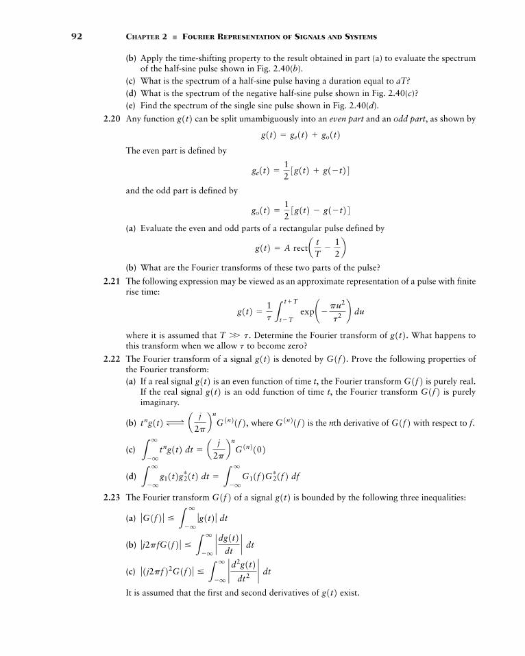
92 CHAPTER 2 � FOURIER REPRESENTATION OF SIGNALS AND SYSTEMS
(b) Apply the time-shifting property to the result obtained in part (a) to evaluate the spectrumof the half-sine pulse shown in Fig. 2.40(b).
(c) What is the spectrum of a half-sine pulse having a duration equal to aT?(d) What is the spectrum of the negative half-sine pulse shown in Fig. 2.40(c)?(e) Find the spectrum of the single sine pulse shown in Fig. 2.40(d).
2.20 Any function can be split umambiguously into an even part and an odd part, as shown by
The even part is defined by
and the odd part is defined by
(a) Evaluate the even and odd parts of a rectangular pulse defined by
(b) What are the Fourier transforms of these two parts of the pulse?
2.21 The following expression may be viewed as an approximate representation of a pulse with finiterise time:
where it is assumed that Determine the Fourier transform of What happens tothis transform when we allow to become zero?
2.22 The Fourier transform of a signal is denoted by Prove the following properties ofthe Fourier transform:(a) If a real signal is an even function of time t, the Fourier transform is purely real.
If the real signal is an odd function of time t, the Fourier transform is purelyimaginary.
(b) where is the nth derivative of with respect to
(c)
(d)
2.23 The Fourier transform of a signal is bounded by the following three inequalities:
(a)
(b)
(c)
It is assumed that the first and second derivatives of exist.g1t2ƒ1j2pf22G1f2 ƒ � L
q
�q` d2g1t2
dt2 ` dt
ƒ j2pfG1f2 ƒ � Lq
�q` dg1t2
dt` dt
ƒG1f2 ƒ � Lq
�qƒg1t2 ƒ dt
g1t2G1f2L
q
�qg11t2g2
…1t2 dt � Lq
�qG11f2G2
…1f2 df
Lq
�qtng1t2 dt � a j
2pb n
G1n2102f.G1f2G1n21f2tng1t2 Δ a j
2pb n
G1n21f2,G1f2g1t2 G1f2g1t2
G1f2.g1t2t
g1t2.T W t.
g1t2 �1t L
tT
t�T exp¢�
pu2
t2 ≤ du
g1t2 � A recta tT
�12b
go1t2 �123g1t2 � g1�t24
ge1t2 �123g1t2 g1�t24
g1t2 � ge1t2 go1t2g1t2
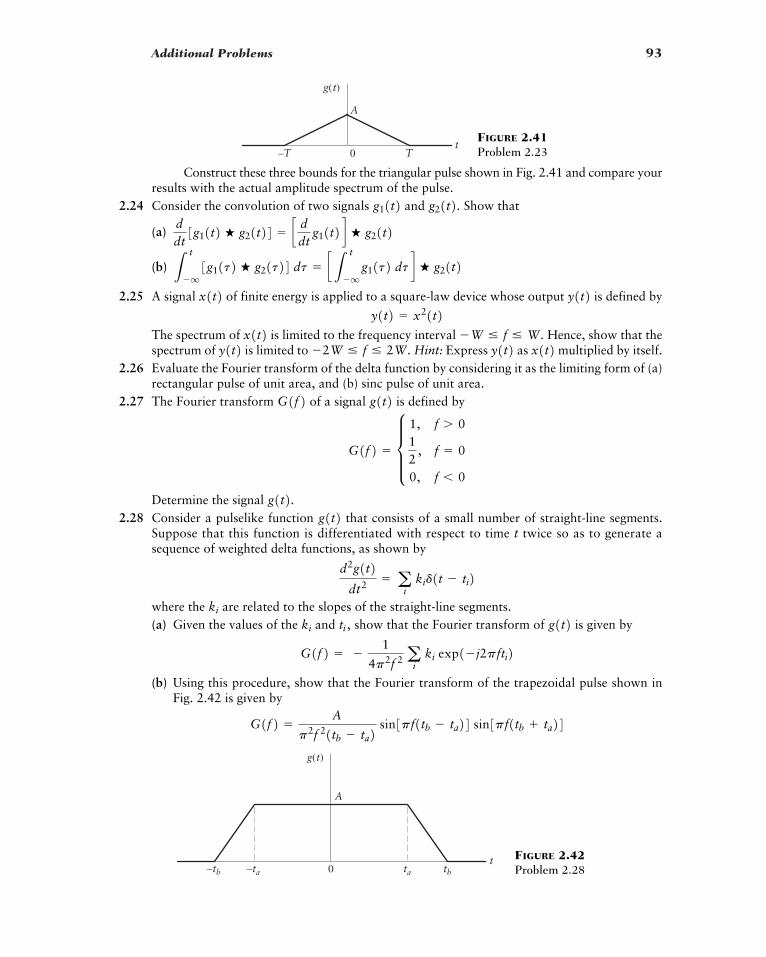
Additional Problems 93
A
–T 0t
g(t)
TFIGURE 2.41Problem 2.23
Construct these three bounds for the triangular pulse shown in Fig. 2.41 and compare yourresults with the actual amplitude spectrum of the pulse.
2.24 Consider the convolution of two signals and Show that
(a)
(b)
2.25 A signal of finite energy is applied to a square-law device whose output is defined by
The spectrum of is limited to the frequency interval Hence, show that thespectrum of is limited to Hint: Express as multiplied by itself.
2.26 Evaluate the Fourier transform of the delta function by considering it as the limiting form of (a)rectangular pulse of unit area, and (b) sinc pulse of unit area.
2.27 The Fourier transform of a signal is defined by
Determine the signal 2.28 Consider a pulselike function that consists of a small number of straight-line segments.
Suppose that this function is differentiated with respect to time t twice so as to generate asequence of weighted delta functions, as shown by
where the are related to the slopes of the straight-line segments.(a) Given the values of the and show that the Fourier transform of is given by
(b) Using this procedure, show that the Fourier transform of the trapezoidal pulse shown inFig. 2.42 is given by
G1f2 �A
p2f 21tb � ta2 sin3pf1tb � ta24 sin3pf1tb ta24
G1f2 � �1
4p2f 2 ai
ki exp1�j2pfti2g1t2ti ,ki
ki
d2g1t2dt2 � a
ikid1t � ti2
g1t2g1t2.
G1f2 � d 1, f � 012
, f � 0
0, f � 0
g1t2G1f2
x1t2y1t2�2W � f � 2W.y1t2 �W � f � W.x1t2y1t2 � x21t2
y1t2x1t2Lt
�q3g11t2 � g21t24 dt � cL
t
�qg11t2 dt d � g21t2
ddt3g11t2 � g21t24 � c d
dtg11t2 d � g21t2
g21t2.g11t2
A
t–tb –ta ta tb0
g(t)
FIGURE 2.42Problem 2.28
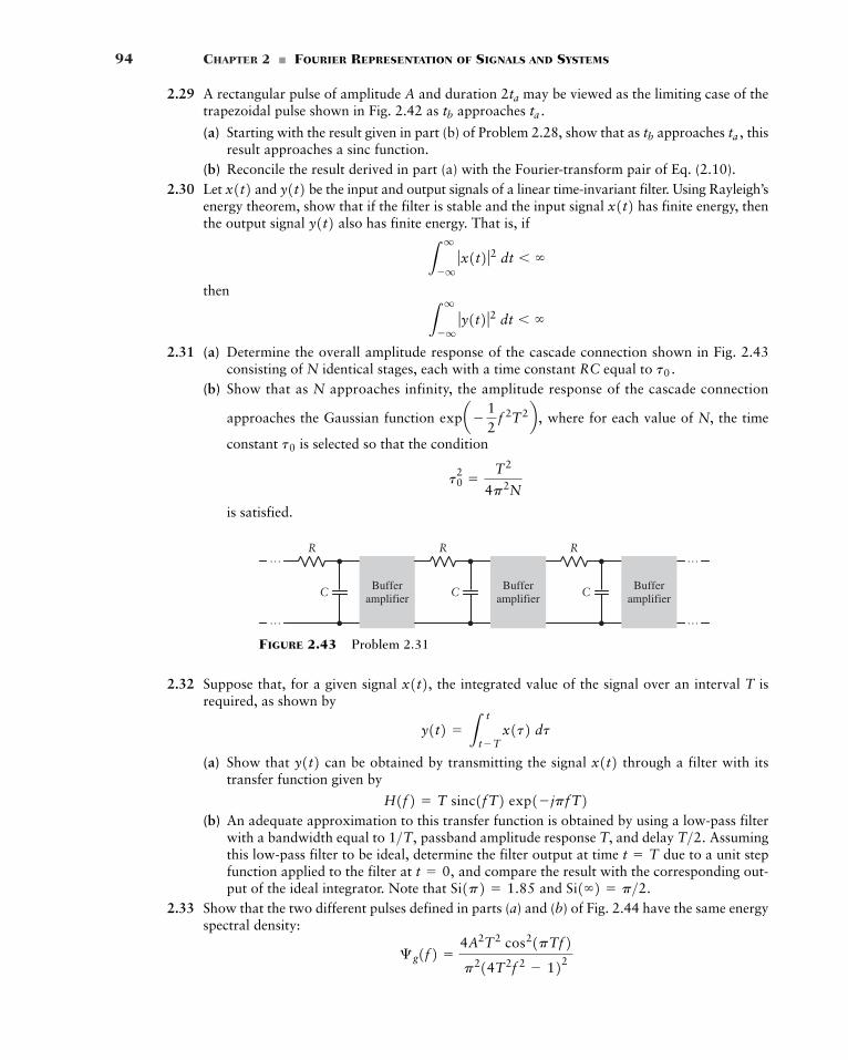
94 CHAPTER 2 � FOURIER REPRESENTATION OF SIGNALS AND SYSTEMS
R
C
…
…
…
…
Bufferamplifier
R
CBuffer
amplifier
R
CBuffer
amplifier
FIGURE 2.43 Problem 2.31
2.29 A rectangular pulse of amplitude A and duration may be viewed as the limiting case of thetrapezoidal pulse shown in Fig. 2.42 as approaches
(a) Starting with the result given in part (b) of Problem 2.28, show that as approaches thisresult approaches a sinc function.
(b) Reconcile the result derived in part (a) with the Fourier-transform pair of Eq. (2.10).2.30 Let and be the input and output signals of a linear time-invariant filter. Using Rayleigh’s
energy theorem, show that if the filter is stable and the input signal has finite energy, thenthe output signal also has finite energy. That is, if
then
2.31 (a) Determine the overall amplitude response of the cascade connection shown in Fig. 2.43consisting of N identical stages, each with a time constant RC equal to
(b) Show that as N approaches infinity, the amplitude response of the cascade connection
approaches the Gaussian function where for each value of N, the time
constant is selected so that the condition
is satisfied.
t02
�T2
4p2N
t0
expa�12
f 2T2b ,
t0 .
Lq
�qƒy1t2 ƒ2 dt � �
Lq
�qƒx1t2 ƒ2 dt � �
y1t2 x1t2y1t2x1t2
ta ,tb
ta .tb2ta
2.32 Suppose that, for a given signal , the integrated value of the signal over an interval T isrequired, as shown by
(a) Show that can be obtained by transmitting the signal through a filter with itstransfer function given by
(b) An adequate approximation to this transfer function is obtained by using a low-pass filterwith a bandwidth equal to passband amplitude response T, and delay Assumingthis low-pass filter to be ideal, determine the filter output at time due to a unit stepfunction applied to the filter at and compare the result with the corresponding out-put of the ideal integrator. Note that and
2.33 Show that the two different pulses defined in parts (a) and (b) of Fig. 2.44 have the same energyspectral density:
°g1f2 �4A2T2 cos21pTf2p214T2f 2 � 122
Si1�2 � p>2.Si1p2 � 1.85t � 0,
t � TT>2.1>T,
H1f2 � T sinc1fT2 exp1�jpfT2x1t2y1t2
y1t2 � Lt
t�Tx1t2 dt
x1t2
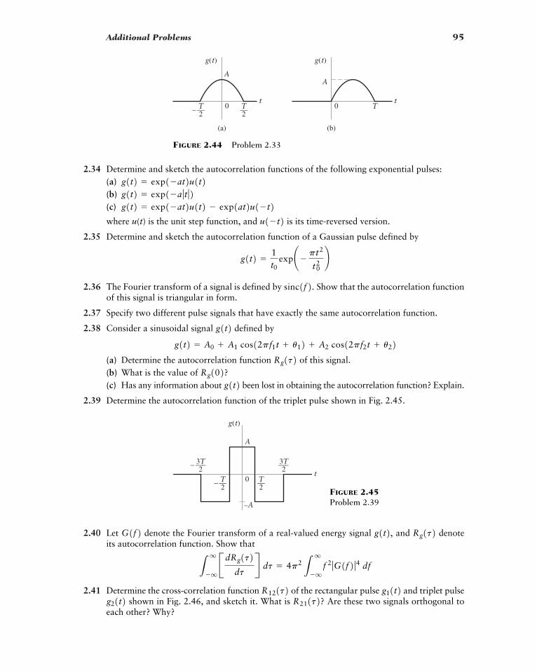
Additional Problems 95
(a) (b)
0
A
t
g(t)
– —T2
—T2
0
A
t
g(t)
T
FIGURE 2.44 Problem 2.33
0
A
t
g(t)
– —T2
– —–3T2
—–3T2
—T2
–A
FIGURE 2.45Problem 2.39
2.34 Determine and sketch the autocorrelation functions of the following exponential pulses:(a)(b)(c)
where u(t) is the unit step function, and is its time-reversed version.
2.35 Determine and sketch the autocorrelation function of a Gaussian pulse defined by
2.36 The Fourier transform of a signal is defined by Show that the autocorrelation functionof this signal is triangular in form.
2.37 Specify two different pulse signals that have exactly the same autocorrelation function.
2.38 Consider a sinusoidal signal defined by
(a) Determine the autocorrelation function of this signal.(b) What is the value of (c) Has any information about been lost in obtaining the autocorrelation function? Explain.
2.39 Determine the autocorrelation function of the triplet pulse shown in Fig. 2.45.
g1t2Rg102?Rg1t2
g1t2 � A0 A1 cos12pf1t u12 A2 cos12pf2t u22g1t2
sinc1f2.g1t2 �
1t0
exp¢�pt2
t02 ≤
u1�t2g1t2 � exp1�at2u1t2 � exp1at2u1�t2g1t2 � exp1�a ƒ t ƒ2g1t2 � exp1�at2u1t2
2.40 Let denote the Fourier transform of a real-valued energy signal and denoteits autocorrelation function. Show that
2.41 Determine the cross-correlation function of the rectangular pulse and triplet pulseshown in Fig. 2.46, and sketch it. What is Are these two signals orthogonal to
each other? Why?R211t2?g21t2 g11t2R121t2
Lq
�qB dRg1t2
dtR dt � 4p2
Lq
�qf 2 ƒG1f2 ƒ4 df
Rg1t2g1t2,G1f2
96 CHAPTER 2 � FOURIER REPRESENTATION OF SIGNALS AND SYSTEMS
0f
Sg(f )
–1 1
1
2
2
–2
FIGURE 2.47Problem 2.44
t (seconds)
g(t)
–1.0
1.0
1–1–3–5–7 3 5 70
... ...
FIGURE 2.48 Problem 2.45
0t
g2(t)
–1.0
1.0
31–1–3
0t
g1(t)
1.0
3–3
FIGURE 2.46 Problem 2.41
2.42 Consider two energy signals and These two signals are delayed by amounts equalto and seconds, respectively. Show that the time delays are additive in convolving the pairof delayed signals, whereas they are subtractive in cross-correlating them.
2.43 (a) An energy signal its Fourier transform autocorrelation function andenergy spectral density are all related, directly or indirectly. Construct a flow-graphthat portrays all the possible direct relationships between them.
(b) If you are given the frequency-domain description the autocorrelation function can be calculated from Outline two ways in which this calculation can be performed.
2.44 Find the autocorrelation function of a power signal whose power spectral density is depictedin Fig. 2.47. What is the value of this autocorrelation function at the origin?
g1t2X1f2. Rx1t2X1f2,°x1f2 Rx1t2,X1f2,x1t2,
t2t1g21t2.g11t2
2.45 Consider the square wave shown in Fig. 2.48. Find the power spectral density, averagepower, and autocorrelation function of this square wave. Does the wave have dc power? Explainyour answer.
g1t2
2.46 Consider two periodic signals and that have the following complex Fourier seriesrepresentations:
gp11t2 � aq
n� ��c1,n exp¢ j2pnt
T0≤
gp21t2gp11t2
Additional Problems 97
and
The two signals have a common period equal to Using the following definition of cross-correlation for a pair of periodic signals,
show that the prescribed pair of periodic signals satisfies the Fourier-transform pair
2.47 A periodic signal of period is represented by the complex Fourier series
where the are the complex Fourier coefficients. The autocorrelation function of isdefined by
(a) Consider the sinusoidal wave
Determine the autocorrelation function and plot its waveform.
(b) Show that
2.48 Repeat parts (a) and (b) of Problem 2.47 for the square wave:
2.49 Determine the power spectral density of (a) the sinusoidal wave of Problem 2.47, and (b) thesquare wave of Problem 2.48.
2.50 Following a procedure similar to that described in Section 2.10 that led to the flow graph ofFig. 2.36 for the 8-point FFT algorithm based on decimation-in-frequency, do the following:
(a) Develop the corresponding flow graph for the 8-point FFT algorithm based on decimation-in-time.
(b) Compare the flow graph obtained in part (a) with that described in Fig. 2.36, stressing thesimilarities and differences between these two basic methods for deriving the FFT algorithm.
gp1t2 � c A, �T0
4� t �
T0
40, for the remainder of period T0
Rgp102 � A2>2.
Rgp1t2
gp1t2 � A cos12pfct u2
Rgp1t2 �
1T0 L
T0>2�T0>2 gp1t2gp
…1t � t2 dt
gp1t2cn
gp1t2 � aq
n� ��cn exp1j2pnt>T02
T0gp1t2R121t2 Δ a
q
n� ��c1, nc2, n
… d¢ f �nT0≤
R121t2 �1T0 L
T0>2�T0>2 gp11t2gp2
… 1t � t2 dt
T0 .
gp21t2 � aq
n� ��c2,n exp¢ j2pnt
T0≤
98 CHAPTER 2 � FOURIER REPRESENTATION OF SIGNALS AND SYSTEMS
ADVANCED PROBLEMS
2.51 (a) The root mean-square (rms) bandwidth of a low-pass signal of finite energy is defined by
where is the energy spectral density of the signal. Correspondingly, the root mean-square (rms) duration of the signal is defined by
Using these definitions, show that
Assume that faster than as
(b) Consider a Gaussian pulse defined by
Show that, for this signal, the equality
can be reached. Hint: Use Schwarz’s inequality (see Appendix 5).
in which we set
and
2.52 The Hilbert transform of a Fourier transformable signal is defined by
Correspondingly, the inverse Hilbert transform is defined by
g1t2 � �1p L
q
�q
gN1t2t � t
dt
gN1t2 �1p L
q
�q
g1t2t � t
dt
g1t2g21t2 �
dg1t2dt
g11t2 � tg1t2
e Lq
�q3g1…1t2g21t2 g11t2g2
…1t24 dt f 2
� 4 Lq
�qƒg11t2 ƒ2 L
q
�qƒg21t2 ƒ2 dt
TrmsWrms �1
4p
g1t2 � exp1�pt22ƒ t ƒ S �.1>2 ƒ t ƒƒg1t2 ƒ S 0
TrmsWrms �1
4p
Trms � D L q
�qt2 ƒg1t2 ƒ2 dt
Lq
�qƒg1t2 ƒ2 dt
T 1>2ƒG1f2 ƒ2
Wrms � D L q
�qf 2 ƒG1f2 ƒ2 df
Lq
�qƒG1f2 ƒ2 df
T 1>2g1t2
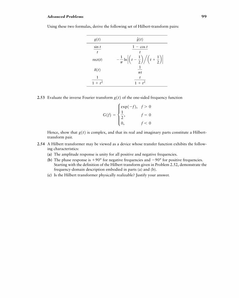
Advanced Problems 99
Using these two formulas, derive the following set of Hilbert-transform pairs:
2.53 Evaluate the inverse Fourier transform of the one-sided frequency function
Hence, show that is complex, and that its real and imaginary parts constitute a Hilbert-transform pair.
2.54 A Hilbert transformer may be viewed as a device whose transfer function exhibits the follow-ing characteristics:(a) The amplitude response is unity for all positive and negative frequencies.(b) The phase response is for negative frequencies and for positive frequencies.
Starting with the definition of the Hilbert transform given in Problem 2.52, demonstrate thefrequency-domain description embodied in parts (a) and (b).
(c) Is the Hilbert transformer physically realizable? Justify your answer.
�90°90°
g1t2
G1f2 � d exp1�f2, f � 012
, f � 0
0, f � 0
g1t2
rect(t)
t
1 t2
1
1 t2
1pt
d1t2�
1p
ln ` a t �12bn at
12b `
1 � cos tt
sin tt
gN1t2g1t2
100
CHAPTER 3
AMPLITUDE MODULATION
Modulation is defined as the process by which some characteristic of a carrier wave is var-ied in accordance with an information-bearing signal. The carrier is needed to facilitate thetransportation of the modulated signal across a band-pass channel from the transmitter tothe receiver. A commonly used carrier is a sinusoidal wave, the source of which is physi-cally independent of the source of the information-bearing signal. When the information-bearing signal is of an analog kind, we speak of continuous-wave modulation, a term thatstresses continuity of the modulated wave as a function of time.
In the context of communications, a primary motivation for modulation is to facili-tate transmission of the information-bearing signal over a communication channel (e.g.,radio channel) with a prescribed passband. In continuous-wave modulation, this is madepossible by varying the amplitude or angle of the sinusoidal carrier wave. On this basis, wemay classify continuous-wave modulation into two broadly defined families: amplitudemodulation and angle modulation. These two families of modulation distinguish them-selves by offering entirely different spectral characteristics and therefore different practicalbenefits. The classification is made on the basis of whether, on the one hand, the amplitudeof the sinusoidal carrier wave, or, on the other hand, the phase or frequency (and there-fore) the angle of the sinusoidal carrier wave, is varied in accordance with the information-bearing signal. The family of amplitude modulation is studied in this chapter, followed bythe study of angle modulation in the next chapter.
In Chapter 1, we identified system complexity and the two primary communicationresources—namely, transmitted power and channel bandwidth—as the central issuesinvolved in the design of a communication system. With these issues in mind, in this chap-ter, we will study four linear modulation strategies that constitute the amplitude modula-tion family:
� amplitude modulation (AM)
� double sideband-suppressed carrier (DSB-SC)
� single sideband (SSB)
� vestigial sideband (VSB)
These four types of modulation differ from each other by virtue of their spectral character-istics. Their study will teach us the following lessons:
� Lesson 1: Fourier analysis provides a powerful mathematical tool for developing mathe-matical as well as physical insight into the spectral characterization of linear modulationstrategies.
3.1 Amplitude Modulation 101
1 Throughout the book, the term “amplitude modulation” or AM, for short, is used to refer to that particular formof modulation in which the carrier wave and both sidebands are present.
� Lesson 2: The implementation of analog communications is significantly simplified byusing AM, at the expense of transmitted power and channel bandwidth.
� Lesson 3: The utilization of transmitted power and channel bandwidth is improvedthrough well-defined modifications of an amplitude-modulated wave’s spectral content atthe expense of increased system complexity.
In short, we may make the statement:
There is no free lunch in designing a communication system: for every gain that is made,there is a price to be paid.
3.1 Amplitude Modulation
� THEORY
Consider a sinusoidal carrier wave defined by
(3.1)
where is the carrier amplitude and is the carrier frequency. The information-bearingsignal or message signal is denoted by m(t); the terms “information-bearing signal” and“message signal” are used interchangeably throughout the book. To simplify the exposi-tion without affecting the results obtained and conclusions reached, we have assumed thatthe phase of the carrier wave is zero in Eq. (3.1). Amplitude modulation1 (AM) is formallydefined as a process in which the amplitude of the carrier wave is varied about a meanvalue, linearly with the message signal An amplitude-modulated (AM) wave maythus be described as a function of time as follows:
(3.2)
where is a constant called the amplitude sensitivity of the modulator responsible for the gen-eration of the modulated signal Typically, the carrier amplitude and the message signal
are measured in volts, in which case the amplitude sensitivity is measured inNotice that if the message signal is switched off, the sinusoidal carrier is left intact.
Figure 3.1(a) shows a message signal and Figs. 3.1(b) and 3.1(c) show the cor-responding AM wave for two values of amplitude sensitivity and a carrier ampli-tude
In amplitude modulation, information pertaining to the message signal residessolely in the envelope, which is defined as the amplitude of the modulated wave —thatis, From this expression, we observe that the envelope of has essen-tially the same shape as the message signal provided that two conditions are satisfied:
1. The amplitude of is always less than unity; that is,
(3.3)
This condition is illustrated in Fig. 3.1(b); it ensures that the function isalways positive, in which case we may express the envelope of the AM wave ofEq. (3.2) simply as When the amplitude sensitivity of thekaAc31 kam1t24. s1t21 kam1t2
ƒkam1t2 ƒ � 1, for all t
kam1t2m1t2 s1t2Ac ƒ1 kam1t2 ƒ . s1t2m1t2Ac � 1 volt.
kas1t2 m1t2,m1t2 volt�1.kam1t2 Acs1t2.ka
s1t2 � Ac31 kam1t24 cos12pfct2m1t2. c1t2
fcAc
c1t2 � Ac cos12pfct2c1t2
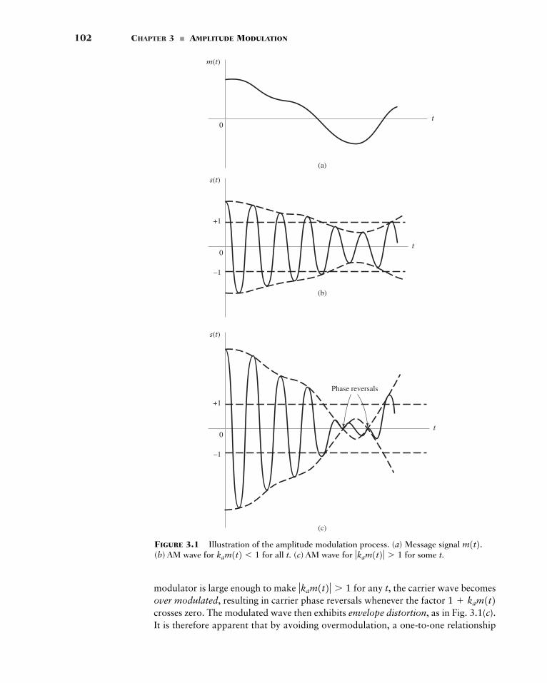
102 CHAPTER 3 � AMPLITUDE MODULATION
(a)
m(t)
0t
(b)
s(t)
0
–1
+1
t
(c)
s(t)
0
–1
+1
t
Phase reversals
FIGURE 3.1 Illustration of the amplitude modulation process. (a) Message signal (b) AM wave for for all t. (c) AM wave for for some t.ƒkam1t2 ƒ � 1kam1t2 � 1
m1t2.
modulator is large enough to make for any t, the carrier wave becomesover modulated, resulting in carrier phase reversals whenever the factor crosses zero. The modulated wave then exhibits envelope distortion, as in Fig. 3.1(c).It is therefore apparent that by avoiding overmodulation, a one-to-one relationship
1 kam1t2ƒkam1t2 ƒ � 1
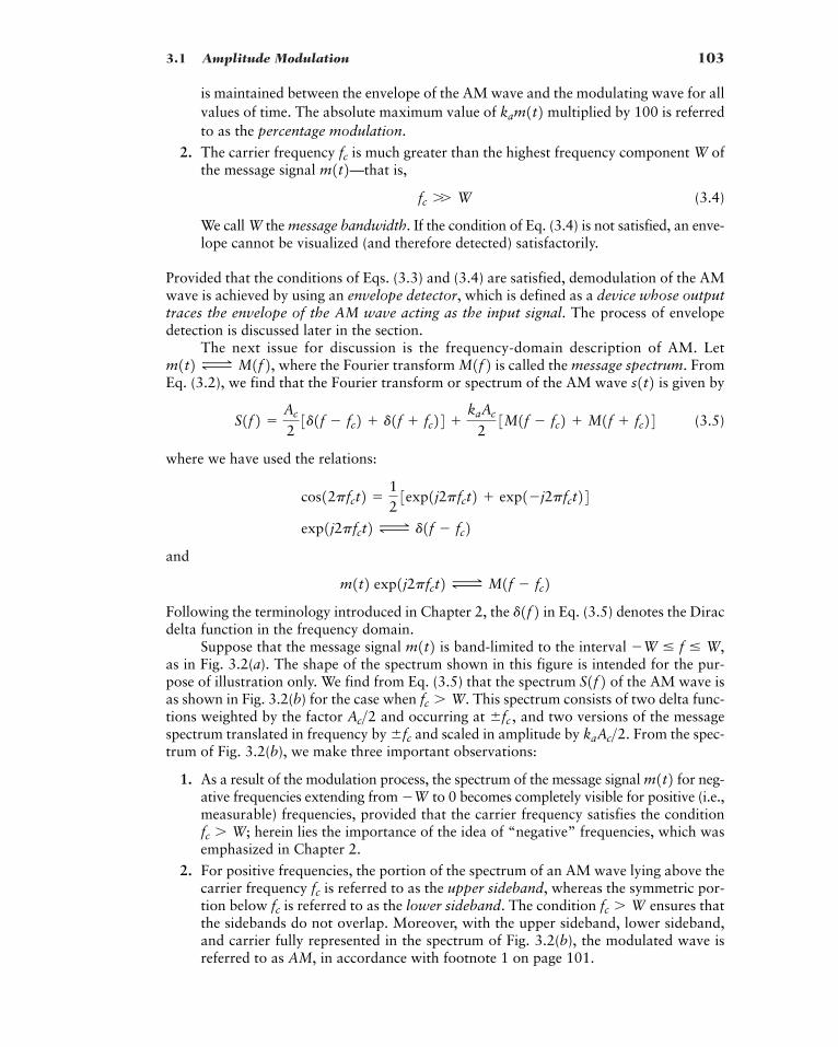
3.1 Amplitude Modulation 103
is maintained between the envelope of the AM wave and the modulating wave for allvalues of time. The absolute maximum value of multiplied by 100 is referredto as the percentage modulation.
2. The carrier frequency is much greater than the highest frequency component W ofthe message signal —that is,
(3.4)
We call W the message bandwidth. If the condition of Eq. (3.4) is not satisfied, an enve-lope cannot be visualized (and therefore detected) satisfactorily.
Provided that the conditions of Eqs. (3.3) and (3.4) are satisfied, demodulation of the AMwave is achieved by using an envelope detector, which is defined as a device whose outputtraces the envelope of the AM wave acting as the input signal. The process of envelopedetection is discussed later in the section.
The next issue for discussion is the frequency-domain description of AM. Letwhere the Fourier transform is called the message spectrum. From
Eq. (3.2), we find that the Fourier transform or spectrum of the AM wave is given by
(3.5)
where we have used the relations:
and
Following the terminology introduced in Chapter 2, the in Eq. (3.5) denotes the Diracdelta function in the frequency domain.
Suppose that the message signal is band-limited to the interval as in Fig. 3.2(a). The shape of the spectrum shown in this figure is intended for the pur-pose of illustration only. We find from Eq. (3.5) that the spectrum of the AM wave isas shown in Fig. 3.2(b) for the case when This spectrum consists of two delta func-tions weighted by the factor and occurring at and two versions of the messagespectrum translated in frequency by and scaled in amplitude by From the spec-trum of Fig. 3.2(b), we make three important observations:
1. As a result of the modulation process, the spectrum of the message signal for neg-ative frequencies extending from to 0 becomes completely visible for positive (i.e.,measurable) frequencies, provided that the carrier frequency satisfies the condition
herein lies the importance of the idea of “negative” frequencies, which wasemphasized in Chapter 2.
2. For positive frequencies, the portion of the spectrum of an AM wave lying above thecarrier frequency is referred to as the upper sideband, whereas the symmetric por-tion below is referred to as the lower sideband. The condition ensures thatthe sidebands do not overlap. Moreover, with the upper sideband, lower sideband,and carrier fully represented in the spectrum of Fig. 3.2(b), the modulated wave isreferred to as AM, in accordance with footnote 1 on page 101.
fc � Wfcfc
fc � W;
�Wm1t2
kaAc>2.�fc�fc ,Ac>2 fc � W.
S1f2�W � f � W,m1t2
d1f2m1t2 exp1j2pfct2 Δ M1f � fc2
exp1j2pfct2 Δ d1f � fc2cos12pfct2 �
123exp1j2pfct2 exp1�j2pfct24
S1f2 �Ac
23d1f � fc2 d1f fc24
kaAc
23M1f � fc2 M1f fc24
s1t2M1f2m1t2 Δ M1f2,
fc W W
m1t2fckam1t2
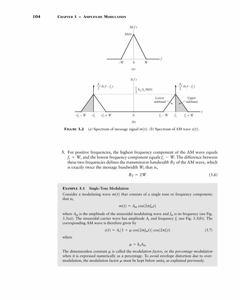
104 CHAPTER 3 � AMPLITUDE MODULATION
M(0)
f
(a)
–W W
M( f )
S( f )
0
0f
(b)
–fc–fc – W –fc + W fc – W fc + Wfc
2
Lowersideband
Uppersideband
1 kaAcM(0) 2Ac �( f – fc)
2Ac �( f – fc)
FIGURE 3.2 (a) Spectrum of message signal (b) Spectrum of AM wave s1t2.m1t2.
3. For positive frequencies, the highest frequency component of the AM wave equalsand the lowest frequency component equals The difference between
these two frequencies defines the transmission bandwidth of the AM wave, whichis exactly twice the message bandwidth W; that is,
(3.6)
EXAMPLE 3.1 Single-Tone Modulation
Consider a modulating wave that consists of a single tone or frequency component; that is,
where is the amplitude of the sinusoidal modulating wave and is its frequency (see Fig.3.3(a)). The sinusoidal carrier wave has amplitude and frequency (see Fig. 3.3(b)). Thecorresponding AM wave is therefore given by
(3.7)
where
The dimensionless constant is called the modulation factor, or the percentage modulationwhen it is expressed numerically as a percentage. To avoid envelope distortion due to over-modulation, the modulation factor must be kept below unity, as explained previously.m
m
m � kaAm
s1t2 � Ac31 m cos12pfmt24 cos12pfct2fcAc
fmAm
m1t2 � Am cos12pfmt2m1t2
BT � 2W
BT
fc � W.fc W,
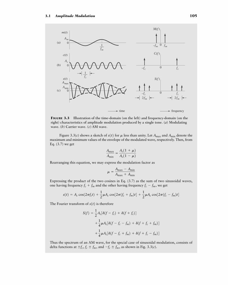
3.1 Amplitude Modulation 105
(a)
m(t)M(f )
Am
0—–1fm
(b)
c(t)
Ac
0
—–1fc
2 fm 2 fm
(c)
s(t)
Amin
Amax
0
time frequency
–fm fm0
C(f )
–fc fc0
S(f )
–fc fc0
FIGURE 3.3 Illustration of the time-domain (on the left) and frequency-domain (on theright) characteristics of amplitude modulation produced by a single tone. (a) Modulatingwave. (b) Carrier wave. (c) AM wave.
Figure 3.3(c) shows a sketch of for less than unity. Let and denote themaximum and minimum values of the envelope of the modulated wave, respectively. Then, fromEq. (3.7) we get
Rearranging this equation, we may express the modulation factor as
Expressing the product of the two cosines in Eq. (3.7) as the sum of two sinusoidal waves,one having frequency and the other having frequency we get
The Fourier transform of is therefore
Thus the spectrum of an AM wave, for the special case of sinusoidal modulation, consists ofdelta functions at and as shown in Fig. 3.3(c).�fc � fm ,�fc , fc � fm ,
14mAc3d1f � fc fm2 d1f fc � fm24
14mAc3d1f � fc � fm2 d1f fc fm24
S1f2 �12
Ac3d1f � fc2 d1f fc24s1t2
s1t2 � Ac cos12pfct2 12mAc cos32p1fc fm2t4
12mAc cos32p1fc � fm2t4fc � fm ,fc fm
m �Amax � Amin
Amax Amin
Amax
Amin�
Ac11 m2Ac11 � m2
AminAmaxms1t2
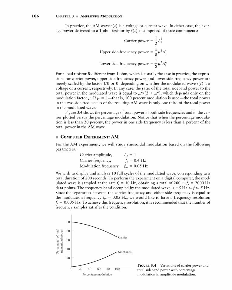
106 CHAPTER 3 � AMPLITUDE MODULATION
In practice, the AM wave is a voltage or current wave. In either case, the aver-age power delivered to a 1-ohm resistor by is comprised of three components:
For a load resistor R different from 1 ohm, which is usually the case in practice, the expres-sions for carrier power, upper side-frequency power, and lower side-frequency power aremerely scaled by the factor 1/R or R, depending on whether the modulated wave is avoltage or a current, respectively. In any case, the ratio of the total sideband power to thetotal power in the modulated wave is equal to which depends only on themodulation factor If —that is, 100 percent modulation is used—the total powerin the two side frequencies of the resulting AM wave is only one-third of the total powerin the modulated wave.
Figure 3.4 shows the percentage of total power in both side frequencies and in the car-rier plotted versus the percentage modulation. Notice that when the percentage modula-tion is less than 20 percent, the power in one side frequency is less than 1 percent of thetotal power in the AM wave.
� COMPUTER EXPERIMENT: AM
For the AM experiment, we will study sinusoidal modulation based on the followingparameters:
Carrier amplitude,Carrier frequency,Modulation frequency,
We wish to display and analyze 10 full cycles of the modulated wave, corresponding to atotal duration of 200 seconds. To perform the experiment on a digital computer, the mod-ulated wave is sampled at the rate obtaining a total of data points. The frequency band occupied by the modulated wave is Since the separation between the carrier frequency and either side frequency is equal tothe modulation frequency we would like to have a frequency resolution
To achieve this frequency resolution, it is recommended that the number offrequency samples satisfies the condition:fr � 0.005 Hz.
fm � 0.05 Hz,
�5 Hz � f � 5 Hz.200 fs � 2000 Hzfs � 10 Hz,
fm � 0.05 Hzfc � 0.4 Hz
Ac � 1
m � 1m.m2>12 m22,
s1t2
Lower side-frequency power �18m2Ac
2
Upper side-frequency power �18m2Ac
2
Carrier power �12
Ac2
s1t2s1t2
0 20 40 60 80 100
Sidebands
Carrier
Percentage modulation
Perc
enta
ge o
f to
tal
tran
smitt
ed p
ower
20
40
60
80
100
FIGURE 3.4 Variations of carrier power andtotal sideband power with percentagemodulation in amplitude modulation.
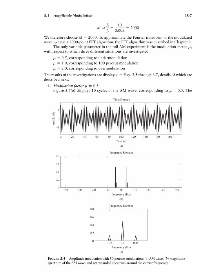
3.1 Amplitude Modulation 107
We therefore choose To approximate the Fourier transform of the modulatedwave, we use a 2000-point FFT algorithm; the FFT algorithm was described in Chapter 2.
The only variable parameter in the full AM experiment is the modulation factor with respect to which three different situations are investigated:
corresponding to undermodulationcorresponding to 100 percent modulationcorresponding to overmodulation
The results of the investigations are displayed in Figs. 3.5 through 3.7, details of which aredescribed next.
1. Modulation factorFigure 3.5(a) displays 10 cycles of the AM wave, corresponding to Them � 0.5.
m � 0.5
m � 2.0,m � 1.0,m � 0.5,
m,
M � 2000.
M �fsfr
�10
0.005� 2000
Am
pltiu
de
Time (s)
0 20 40 60 80 100 120 140 160 180
–1
0
1
–4.0 –2.0–3.0 –1.0 0 1.0 3.02.0 4.00
0.2
0.4
0.6
0.8
Frequency (Hz)
Frequency (Hz)
0.450.40.350
0.2
0.4
0.6
0.8Frequency Domain
Frequency Domain
Time Domain
(a)
(b)
(c)
FIGURE 3.5 Amplitude modulation with 50 percent modulation: (a) AM wave, (b) magnitudespectrum of the AM wave, and (c) expanded spectrum around the carrier frequency.
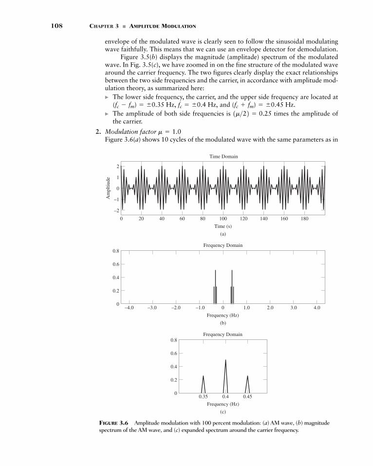
108 CHAPTER 3 � AMPLITUDE MODULATION
envelope of the modulated wave is clearly seen to follow the sinusoidal modulatingwave faithfully. This means that we can use an envelope detector for demodulation.
Figure 3.5(b) displays the magnitude (amplitade) spectrum of the modulatedwave. In Fig. 3.5(c), we have zoomed in on the fine structure of the modulated wavearound the carrier frequency. The two figures clearly display the exact relationshipsbetween the two side frequencies and the carrier, in accordance with amplitude mod-ulation theory, as summarized here:� The lower side frequency, the carrier, and the upper side frequency are located at
and� The amplitude of both side frequencies is times the amplitude of
the carrier.
2. Modulation factorFigure 3.6(a) shows 10 cycles of the modulated wave with the same parameters as in
m � 1.0
1m>22 � 0.25(fc fm) � �0.45 Hz.(fc � fm) � �0.35 Hz, fc � �0.4 Hz,
Am
pltiu
de
Time (s)
0 20 40 60 80 100 120 140 160 180
–2
–1
0
1
2
0
0.2
0.4
0.6
0.8
0
0.2
0.4
0.6
0.8Frequency Domain
Frequency Domain
Time Domain
(a)
(b)
(c)
–4.0 –2.0–3.0 –1.0 0 1.0 3.02.0 4.0
Frequency (Hz)
Frequency (Hz)
0.450.40.35
FIGURE 3.6 Amplitude modulation with 100 percent modulation: (a) AM wave, (b) magnitudespectrum of the AM wave, and (c) expanded spectrum around the carrier frequency.
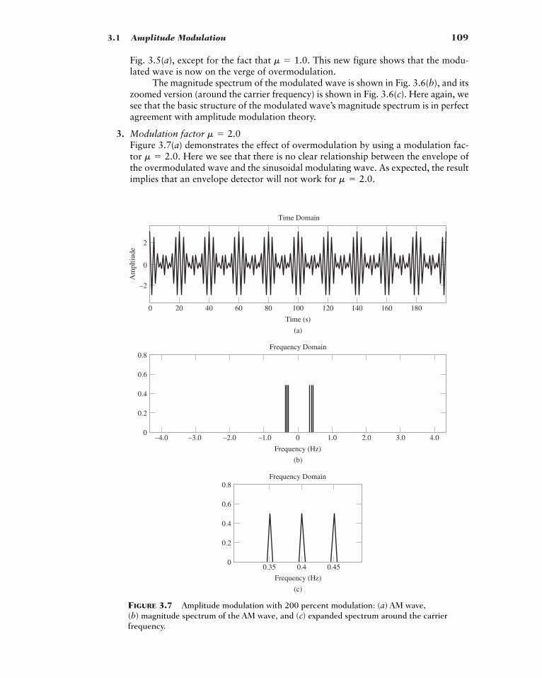
3.1 Amplitude Modulation 109
Fig. 3.5(a), except for the fact that This new figure shows that the modu-lated wave is now on the verge of overmodulation.
The magnitude spectrum of the modulated wave is shown in Fig. 3.6(b), and itszoomed version (around the carrier frequency) is shown in Fig. 3.6(c). Here again, wesee that the basic structure of the modulated wave’s magnitude spectrum is in perfectagreement with amplitude modulation theory.
3. Modulation factorFigure 3.7(a) demonstrates the effect of overmodulation by using a modulation fac-tor Here we see that there is no clear relationship between the envelope ofthe overmodulated wave and the sinusoidal modulating wave. As expected, the resultimplies that an envelope detector will not work for m � 2.0.
m � 2.0.
m � 2.0
m � 1.0.
Am
pltiu
de
Time (s)
0 20 40 60 80 100 120 140 160 180
–2
0
2
Time Domain
(a)
0
0.2
0.4
0.6
0.8
0
0.2
0.4
0.6
0.8Frequency Domain
Frequency Domain
(b)
(c)
–4.0 –2.0–3.0 –1.0 0 1.0 3.02.0 4.0
Frequency (Hz)
Frequency (Hz)
0.450.40.35
FIGURE 3.7 Amplitude modulation with 200 percent modulation: (a) AM wave,(b) magnitude spectrum of the AM wave, and (c) expanded spectrum around the carrierfrequency.
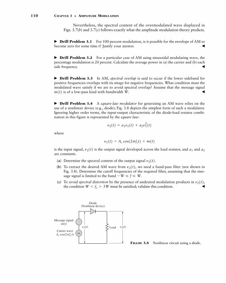
110 CHAPTER 3 � AMPLITUDE MODULATION
Load
Diode(Nonlinear device)
Message signalm(t)
Carrier waveAc cos(2�fc t)
v1(t)
~v2(t)
FIGURE 3.8 Nonlinear circuit using a diode.
Nevertheless, the spectral content of the overmodulated wave displayed inFigs. 3.7(b) and 3.7(c) follows exactly what the amplitude modulation theory predicts.
� Drill Problem 3.1 For 100 percent modulation, is it possible for the envelope of AM tobecome zero for some time t? Justify your answer. �
� Drill Problem 3.2 For a particular case of AM using sinusoidal modulating wave, thepercentage modulation is 20 percent. Calculate the average power in (a) the carrier and (b) eachside frequency. �
� Drill Problem 3.3 In AM, spectral overlap is said to occur if the lower sideband forpositive frequencies overlaps with its image for negative frequencies. What condition must themodulated wave satisfy if we are to avoid spectral overlap? Assume that the message signal
is of a low-pass kind with bandwidth W. �
� Drill Problem 3.4 A square-law modulator for generating an AM wave relies on theuse of a nonlinear device (e.g., diode); Fig. 3.8 depicts the simplest form of such a modulator.Ignoring higher order terms, the input-output characteristic of the diode-load resistor combi-nation in this figure is represented by the square law:
where
is the input signal, is the output signal developed across the load resistor, and and are constants.
(a) Determine the spectral content of the output signal
(b) To extract the desired AM wave from we need a band-pass filter (not shown inFig. 3.8). Determine the cutoff frequencies of the required filter, assuming that the mes-sage signal is limited to the band
(c) To avoid spectral distortion by the presence of undesired modulation products in the condition must be satisfied; validate this condition. �W � fc � 3W
n21t2,�W � f � W.
n21t2,n21t2.
a2a1n21t2n11t2 � Ac cos12pfct2 m1t2
n21t2 � a1n11t2 a2n121t2
m1t2
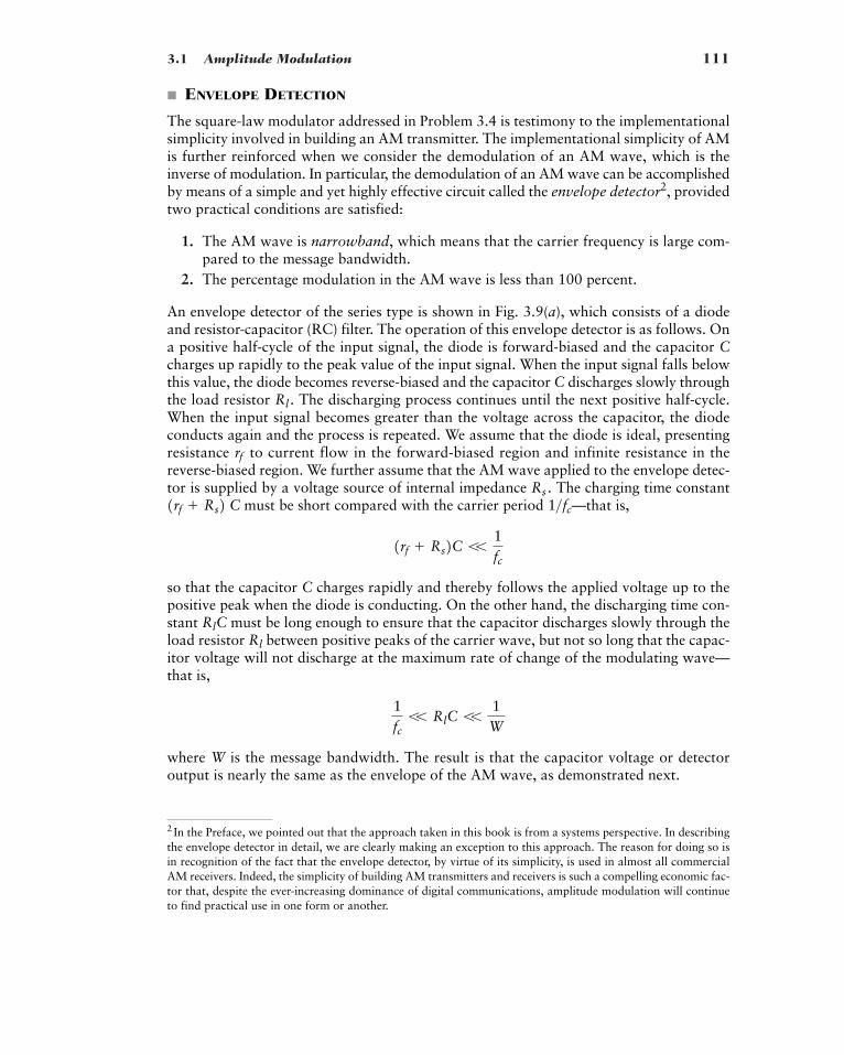
3.1 Amplitude Modulation 111
2 In the Preface, we pointed out that the approach taken in this book is from a systems perspective. In describingthe envelope detector in detail, we are clearly making an exception to this approach. The reason for doing so isin recognition of the fact that the envelope detector, by virtue of its simplicity, is used in almost all commercialAM receivers. Indeed, the simplicity of building AM transmitters and receivers is such a compelling economic fac-tor that, despite the ever-increasing dominance of digital communications, amplitude modulation will continueto find practical use in one form or another.
� ENVELOPE DETECTION
The square-law modulator addressed in Problem 3.4 is testimony to the implementationalsimplicity involved in building an AM transmitter. The implementational simplicity of AMis further reinforced when we consider the demodulation of an AM wave, which is theinverse of modulation. In particular, the demodulation of an AM wave can be accomplishedby means of a simple and yet highly effective circuit called the envelope detector2, providedtwo practical conditions are satisfied:
1. The AM wave is narrowband, which means that the carrier frequency is large com-pared to the message bandwidth.
2. The percentage modulation in the AM wave is less than 100 percent.
An envelope detector of the series type is shown in Fig. 3.9(a), which consists of a diodeand resistor-capacitor (RC) filter. The operation of this envelope detector is as follows. Ona positive half-cycle of the input signal, the diode is forward-biased and the capacitor Ccharges up rapidly to the peak value of the input signal. When the input signal falls belowthis value, the diode becomes reverse-biased and the capacitor C discharges slowly throughthe load resistor The discharging process continues until the next positive half-cycle.When the input signal becomes greater than the voltage across the capacitor, the diodeconducts again and the process is repeated. We assume that the diode is ideal, presentingresistance to current flow in the forward-biased region and infinite resistance in thereverse-biased region. We further assume that the AM wave applied to the envelope detec-tor is supplied by a voltage source of internal impedance The charging time constant
C must be short compared with the carrier period —that is,
so that the capacitor C charges rapidly and thereby follows the applied voltage up to thepositive peak when the diode is conducting. On the other hand, the discharging time con-stant must be long enough to ensure that the capacitor discharges slowly through theload resistor between positive peaks of the carrier wave, but not so long that the capac-itor voltage will not discharge at the maximum rate of change of the modulating wave—that is,
where W is the message bandwidth. The result is that the capacitor voltage or detectoroutput is nearly the same as the envelope of the AM wave, as demonstrated next.
1fc
V RlC V1W
Rl
RlC
1rf Rs2C V1fc
1>fc1rf Rs2 Rs .
rf
Rl .
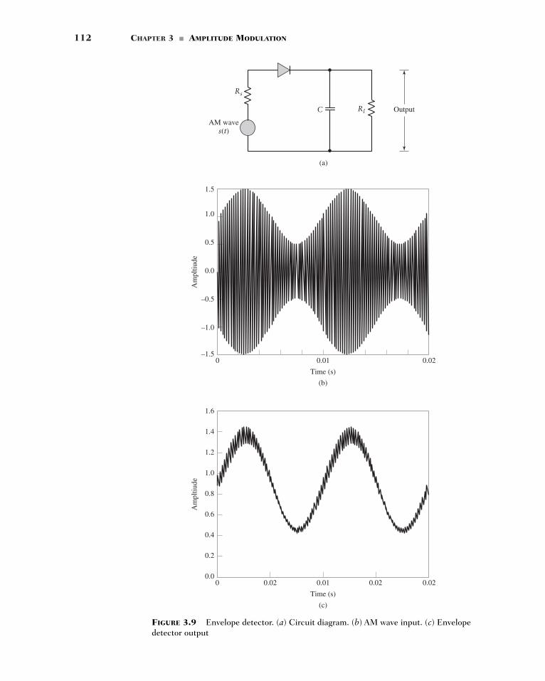
112 CHAPTER 3 � AMPLITUDE MODULATION
Rs
Rl
(a)
AM waves(t)
OutputC
Am
pltiu
de
Time (s)
0 0.01 0.02
–1.0
–0.5
0.0
0.5
1.0
1.5
–1.5
(b)
(c)
Am
pltiu
de
Time (s)
0 0.01 0.020.020.02
0.2
0.4
0.6
0.8
1.0
1.2
1.4
1.6
0.0
FIGURE 3.9 Envelope detector. (a) Circuit diagram. (b) AM wave input. (c) Envelopedetector output
3.2 Virtues, Limitation and Modifications of Amplitude Modulation 113
� COMPUTER EXPERIMENT: ENVELOPE DETECTION FOR SINUSOIDAL AM
Consider the sinusoidal AM wave shown in Fig. 3.9(b), assuming 50 percent modulation.The envelope detector output is shown in Fig. 3.9(c). This latter waveform is computedassuming that the diode is ideal, having a constant resistance when forward-biased andinfinite resistance when reverse-biased. The numerical values used in the computation ofFig. 3.9(c) are as follows:
Source resistanceForward resistanceLoad resistanceCapacitanceMessage bandwidthCarrier frequency
Notice that the envelope detector output includes a high-frequency ripple; this ripple canbe removed by using a low-pass filter (not shown in Fig. 3.9 (a))
3.2 Virtues, Limitations, and Modificationsof Amplitude Modulation
Amplitude modulation is the oldest method of performing modulation. As already remarkedin Section 3.1, its biggest virtue is the ease with which it is generated and reversed. The netresult is that an amplitude modulation system is relatively inexpensive to build.
However, from Chapter 1 we recall that transmitted power and channel bandwidthare our two primary communication resources and they should be used efficiently. In thiscontext, we find that the amplitude modulation defined in Eq. (3.2) suffers from two majorpractical limitations:
1. Amplitude modulation is wasteful of transmitted power. The carrier wave c(t) is com-pletely independent of the information-bearing signal The transmission of thecarrier wave therefore represents a waste of power, which means that in amplitudemodulation only a fraction of the total transmitted power is actually affected by
2. Amplitude modulation is wasteful of channel bandwidth. The upper and lower side-bands of an AM wave are uniquely related to each other by virtue of their symmetry aboutthe carrier frequency; hence, given the amplitude and phase spectra of either sideband,we can uniquely determine the other. This means that insofar as the transmission ofinformation is concerned, only one sideband is necessary, and the communication chan-nel therefore needs to provide only the same bandwidth as the message signal. In lightof this observation, amplitude modulation is wasteful of channel bandwidth as it requiresa transmission bandwidth equal to twice the message bandwidth.
To overcome these two limitations of AM, we must make certain changes that result inincreased system complexity of the amplitude modulation process. In effect, we trade offsystem complexity for improved utilization of communication resources. Starting withamplitude modulation, we can distinguish three modifications of amplitude modulation:
1. Double sideband-suppressed carrier (DSB-SC) modulation, in which the transmittedwave consists of only the upper and lower sidebands. Transmitted power is savedhere through the suppression of the carrier wave, but the channel bandwidth require-ment is the same as before (i.e., twice the message bandwidth).
2. Single sideband (SSB) modulation, in which the modulated wave consists only of theupper sideband or the lower sideband. The essential function of SSB modulation istherefore to translate the spectrum of the modulating signal (with or without inversion)
m1t2.m1t2.
fc � 20 kHzW � 1 kHzC � 0.01 mFRl � 10 kÆrf � 25 Æ
Rs � 75 Æ
rf
114 CHAPTER 3 � AMPLITUDE MODULATION
to a new location in the frequency domain. Single sideband modulation is particularlysuited for the transmission of voice signals by virtue of the energy gap that exists inthe spectrum of voice signals between zero and a few hundred hertz. SSB is the opti-mum form of continuous-wave modulation in that it requires the minimum trans-mitted power and minimum channel bandwidth; its principal disadvantages areincreased complexity and limited applicability.
3. Vestigial sideband (VSB) modulation, in which one sideband is passed almost com-pletely and just a trace, or vestige, of the other sideband is retained. The requiredchannel bandwidth is therefore slightly in excess of the message bandwidth by anamount equal to the width of the vestigial sideband. This form of modulation is wellsuited for the transmission of wideband signals such as television signals that containsignificant components at extremely low frequencies. In commercial television broad-casting, a sizable carrier is transmitted together with the modulated wave, whichmakes it possible to demodulate the incoming modulated signal by an envelope detec-tor in the receiver and thereby simplify the receiver design.
In Section 3.3 we discuss DSB-SC modulation, followed by discussions of SSB and VSBforms of modulation in subsequent sections and in that order.
3.3 Double Sideband-Suppressed Carrier Modulation
� THEORY
Basically, double sideband-suppressed carrier (DSB-SC) modulation consists of the prod-uct of the message signal and the carrier wave as shown in the equation
(3.8)
Accordingly, the device used to generate the DSB-SC modulated wave is referred to as aproduct modulator. From Eq. (3.8) we also note that unlike amplitude modulation, DSB-SCmodulation is reduced to zero whenever the message signal is switched off.
Most noticeably, however, is the fact that the modulated signal undergoes a phasereversal whenever the message signal crosses zero, as indicated in Fig. 3.10(b) for themessage signal depicted in part (a) of the figure. The envelope of a DSB-SC modulatedsignal is therefore different from the message signal, which means that simple demodula-tion using an envelope detection is not a viable option for DSB-SC modulation.
From Eq. (3.8), the Fourier transform of is obtained as
(3.9)
where For the case when the message signal is limited to the inter-val as in Fig. 3.11(a), we find that the spectrum of the DSB-SC wave
is as illustrated in Fig. 3.11(b). Except for a change in scale factor, the modulationprocess simply translates the spectrum of the message signal by to the right and by to the left. Of course, the transmission bandwidth required by DSB-SC modulation is thesame as that for amplitude modulation—namely, 2W.
In short, insofar as bandwidth occupancy is concerned, DSB-SC offers no advantageover AM. Its only advantage lies in saving transmitted power, which is important enoughwhen the available transmitted power is at a premium.
�fcfcs1t2 S1f2�W � f � W,
m1t2m1t2 Δ M1f2.S1f2 �
12
Ac3M1f � fc2 M1f fc24s1t2
m1t2 m1t2 s1t2m1t2
� Ac cos12pfct2m1t2s1t2 � c1t2m1t2
c1t2,m1t2
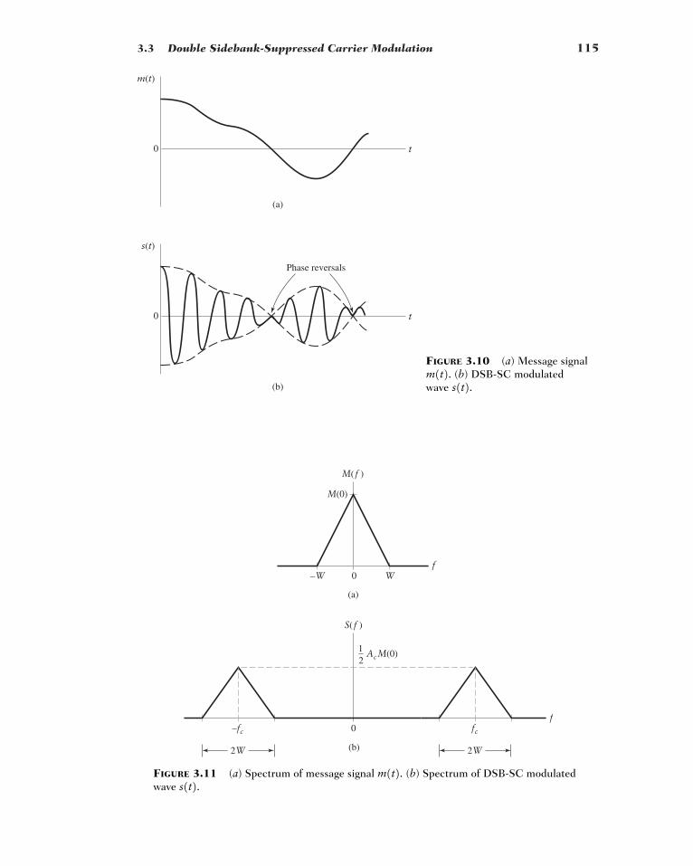
3.3 Double Sidebank-Suppressed Carrier Modulation 115
(a)
m(t)
t0
(b)
s(t)
t0
Phase reversals
FIGURE 3.10 (a) Message signal(b) DSB-SC modulated
wave s1t2.m1t2.
M(0)
f
(a)
–W
2W
W
M( f )
S( f )
0
0f
(b)
–fc fc
21 AcM(0)
2W
FIGURE 3.11 (a) Spectrum of message signal (b) Spectrum of DSB-SC modulatedwave s1t2. m1t2.
116 CHAPTER 3 � AMPLITUDE MODULATION
EXAMPLE 3.2 Sinusoidal DSB-SC spectrum
Consider DSB-SC modulation using a sinusoidal modulating wave of amplitude and fre-quency and operating on a carrier of amplitude and frequency The message spectrum is
Invoking Eq. (3.9), the shifted spectrum defines the two side-frequencies for pos-itive frequencies:
The other shifted spectrum of Eq. (3.9)—namely, —defines the remaining twoside-frequencies for negative frequencies:
which are the images of the first two side-frequencies with respect to the origin, in reverseorder.
� Drill Problem 3.5 For the sinusoidal DSB-SC modulation considered in Example 3.2,what is the average power in the lower or upper side-frequency, expressed as a percentage ofthe average power in the DSB-SC modulated wave? �
� COHERENT DETECTION
Since the envelope of the DSB-SC modulated wave is different from the message signalwe have to find some other means for recovering from To this end, we rec-
ognize that contains a constant term, as shown by the trigonometric identity
In light of this relation rewritten for we see from Eq. (3.8) that the recovery ofthe message signal can be accomplished by first multiplying with a locally gen-erated sinusoidal wave and then low-pass filtering the product. It is assumed that the localoscillator signal is exactly coherent or synchronized, in both frequency and phase, withthe carrier wave used in the product modulator to generate This method ofdemodulation is known as coherent detection or synchronous demodulation.
It is instructive to derive coherent detection as a special case of the more generaldemodulation process using a local oscillator signal of the same frequency but arbitraryphase difference measured with respect to the carrier wave Thus, denoting the localoscillator signal by and using Eq. (3.8) for the DSB-SC wave wefind that the product modulator output in Fig. 3.12 is
(3.10)�12
AcAœc cos14pfct f2m1t2
12
AcA�c cos1f2m1t2� AcA
œc cos12pfct2 cos12pfct f2m1t2
n1t2 � Aœc cos12pfct f2s1t2
s1t2,Aœc cos12pfct f2 c1t2.f,
s1t2.c1t2s1t2m1t2 u � 2pfct,
cos21u2 �12
12
cos12u2cos212pfct2 s1t2.m1t2m1t2, s1t2
14
AcAmd1f 1fc � fm22; 14
AcAmd1f 1fc fm22
12 AcM1f fc2,
14
AcAmd1f � 1fc fm22; 14
AcAmd1f � 1fc � fm22
12 AcM1f � fc2
M1f2 �12
Amd1f � fm2 12
Amd1f fm2fc .Acfm
Am
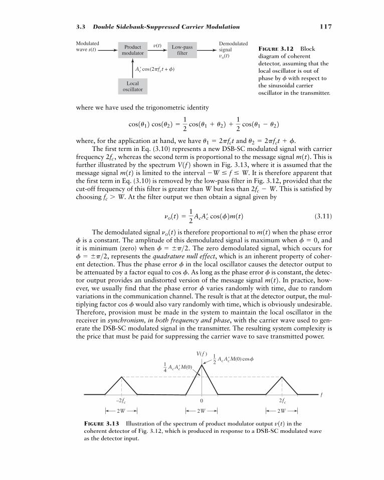
3.3 Double Sidebank-Suppressed Carrier Modulation 117
Ac� cos(2�fct + �)
Modulatedwave s(t) Product
modulator
Localoscillator
Low-passfilter
Demodulatedsignalvo(t)
v(t) FIGURE 3.12 Blockdiagram of coherentdetector, assuming that thelocal oscillator is out ofphase by with respect tothe sinusoidal carrieroscillator in the transmitter.
f
where we have used the trigonometric identity
where, for the application at hand, we have and The first term in Eq. (3.10) represents a new DSB-SC modulated signal with carrier
frequency whereas the second term is proportional to the message signal This isfurther illustrated by the spectrum shown in Fig. 3.13, where it is assumed that themessage signal is limited to the interval It is therefore apparent thatthe first term in Eq. (3.10) is removed by the low-pass filter in Fig. 3.12, provided that thecut-off frequency of this filter is greater than W but less than This is satisfied bychoosing At the filter output we then obtain a signal given by
(3.11)
The demodulated signal is therefore proportional to when the phase erroris a constant. The amplitude of this demodulated signal is maximum when and
it is minimum (zero) when The zero demodulated signal, which occurs forrepresents the quadrature null effect, which is an inherent property of coher-
ent detection. Thus the phase error in the local oscillator causes the detector output tobe attenuated by a factor equal to As long as the phase error is constant, the detec-tor output provides an undistorted version of the message signal In practice, how-ever, we usually find that the phase error varies randomly with time, due to randomvariations in the communication channel. The result is that at the detector output, the mul-tiplying factor would also vary randomly with time, which is obviously undesirable.Therefore, provision must be made in the system to maintain the local oscillator in thereceiver in synchronism, in both frequency and phase, with the carrier wave used to gen-erate the DSB-SC modulated signal in the transmitter. The resulting system complexity isthe price that must be paid for suppressing the carrier wave to save transmitted power.
cos f
f
m1t2.fcos f.f
f � �p>2,f � �p>2.
f � 0,f
m1t2no1t2no1t2 �
12
AcA�c cos1f2m1t2fc � W.
2fc � W.
�W � f � W.m1t2 V1f2 m1t2.2fc ,
u2 � 2pfct f.u1 � 2pfct
cos1u12 cos1u22 �12
cos1u1 u22 12
cos1u1 � u22
V(f )
f0 2fc–2fc
21 AcAc�M(0) cos �
41 AcAc�M(0)
2W 2W 2W
FIGURE 3.13 Illustration of the spectrum of product modulator output in thecoherent detector of Fig. 3.12, which is produced in response to a DSB-SC modulated waveas the detector input.
v1t2
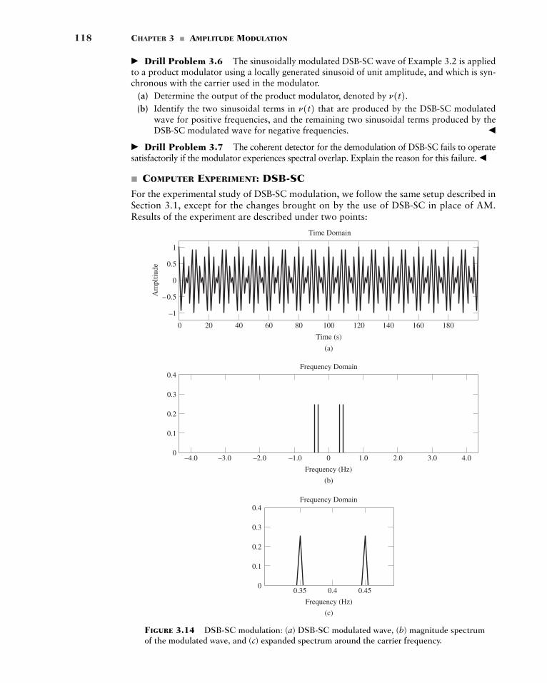
118 CHAPTER 3 � AMPLITUDE MODULATION
Am
pltiu
de
Time (s)
0 20 40 60 80 100 120 140 160 180
–1
–0.5
0
0.5
1
Time Domain
(a)
–4.0 –2.0–3.0 –1.0 0 1.0 3.02.0 4.00
0.1
0.2
0.3
0.4
Frequency (Hz)
Frequency (Hz)
0.450.40.350
0.1
0.2
0.3
0.4Frequency Domain
Frequency Domain
(b)
(c)
FIGURE 3.14 DSB-SC modulation: (a) DSB-SC modulated wave, (b) magnitude spectrumof the modulated wave, and (c) expanded spectrum around the carrier frequency.
� Drill Problem 3.6 The sinusoidally modulated DSB-SC wave of Example 3.2 is appliedto a product modulator using a locally generated sinusoid of unit amplitude, and which is syn-chronous with the carrier used in the modulator.
(a) Determine the output of the product modulator, denoted by (b) Identify the two sinusoidal terms in that are produced by the DSB-SC modulated
wave for positive frequencies, and the remaining two sinusoidal terms produced by theDSB-SC modulated wave for negative frequencies. �
� Drill Problem 3.7 The coherent detector for the demodulation of DSB-SC fails to operatesatisfactorily if the modulator experiences spectral overlap. Explain the reason for this failure. �
� COMPUTER EXPERIMENT: DSB-SCFor the experimental study of DSB-SC modulation, we follow the same setup described inSection 3.1, except for the changes brought on by the use of DSB-SC in place of AM.Results of the experiment are described under two points:
n1t2 n1t2.
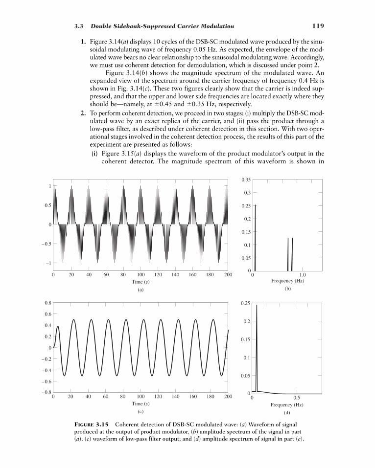
3.3 Double Sidebank-Suppressed Carrier Modulation 119
1. Figure 3.14(a) displays 10 cycles of the DSB-SC modulated wave produced by the sinu-soidal modulating wave of frequency 0.05 Hz. As expected, the envelope of the mod-ulated wave bears no clear relationship to the sinusoidal modulating wave. Accordingly,we must use coherent detection for demodulation, which is discussed under point 2.
Figure 3.14(b) shows the magnitude spectrum of the modulated wave. Anexpanded view of the spectrum around the carrier frequency of frequency 0.4 Hz isshown in Fig. 3.14(c). These two figures clearly show that the carrier is indeed sup-pressed, and that the upper and lower side frequencies are located exactly where theyshould be—namely, at and respectively.
2. To perform coherent detection, we proceed in two stages: (i) multiply the DSB-SC mod-ulated wave by an exact replica of the carrier, and (ii) pass the product through alow-pass filter, as described under coherent detection in this section. With two oper-ational stages involved in the coherent detection process, the results of this part of theexperiment are presented as follows:(i) Figure 3.15(a) displays the waveform of the product modulator’s output in the
coherent detector. The magnitude spectrum of this waveform is shown in
�0.35 Hz,�0.45
0 0.50
0.05
0.1
0.15
0.2
0.25
Frequency (Hz)0 1.0
0
0.05
0.1
0.15
0.2
0.25
0.3
0.35
Time (s)0 20 40 60 80 100 120 140 160 180 200
–0.8
–0.6
–0.4
–0.2
0
0.2
0.4
0.6
0.8
Time (s)0 20 40 60 80 100 120 140 160 180 200
–1
–0.5
0
0.5
1
(b)
Frequency (Hz)
(d)(c)
(a)
FIGURE 3.15 Coherent detection of DSB-SC modulated wave: (a) Waveform of signalproduced at the output of product modulator, (b) amplitude spectrum of the signal in part(a); (c) waveform of low-pass filter output; and (d) amplitude spectrum of signal in part (c).
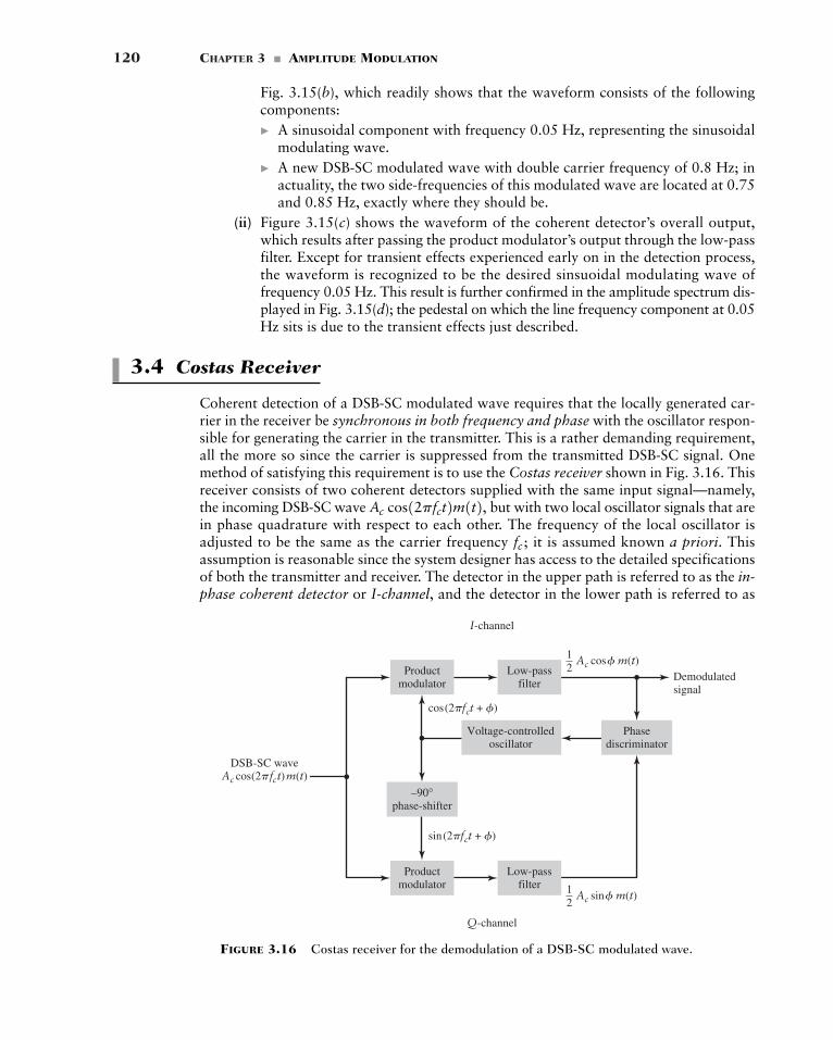
120 CHAPTER 3 � AMPLITUDE MODULATION
Fig. 3.15(b), which readily shows that the waveform consists of the followingcomponents:� A sinusoidal component with frequency 0.05 Hz, representing the sinusoidal
modulating wave.� A new DSB-SC modulated wave with double carrier frequency of 0.8 Hz; in
actuality, the two side-frequencies of this modulated wave are located at 0.75and 0.85 Hz, exactly where they should be.
(ii) Figure 3.15(c) shows the waveform of the coherent detector’s overall output,which results after passing the product modulator’s output through the low-passfilter. Except for transient effects experienced early on in the detection process,the waveform is recognized to be the desired sinsuoidal modulating wave offrequency 0.05 Hz. This result is further confirmed in the amplitude spectrum dis-played in Fig. 3.15(d); the pedestal on which the line frequency component at 0.05Hz sits is due to the transient effects just described.
3.4 Costas Receiver
Coherent detection of a DSB-SC modulated wave requires that the locally generated car-rier in the receiver be synchronous in both frequency and phase with the oscillator respon-sible for generating the carrier in the transmitter. This is a rather demanding requirement,all the more so since the carrier is suppressed from the transmitted DSB-SC signal. Onemethod of satisfying this requirement is to use the Costas receiver shown in Fig. 3.16. Thisreceiver consists of two coherent detectors supplied with the same input signal—namely,the incoming DSB-SC wave but with two local oscillator signals that arein phase quadrature with respect to each other. The frequency of the local oscillator isadjusted to be the same as the carrier frequency it is assumed known a priori. Thisassumption is reasonable since the system designer has access to the detailed specificationsof both the transmitter and receiver. The detector in the upper path is referred to as the in-phase coherent detector or I-channel, and the detector in the lower path is referred to as
fc ;
Ac cos12pfct2m1t2,
cos(2�fct + �)
sin(2�fct + �)
Productmodulator
–90°phase-shifter
DSB-SC waveAc cos(2�fct)m(t)
Q-channel
I-channel
Productmodulator
Low-passfilter
Low-passfilter
Voltage-controlledoscillator
Phasediscriminator
Demodulatedsignal
21 Ac cos� m(t)
21 Ac sin� m(t)
FIGURE 3.16 Costas receiver for the demodulation of a DSB-SC modulated wave.
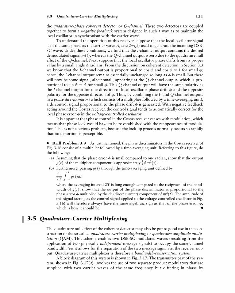
3.5 Quadrature-Carrier Multiplexing 121
the quadrature-phase coherent detector or Q-channel. These two detectors are coupledtogether to form a negative feedback system designed in such a way as to maintain thelocal oscillator in synchronism with the carrier wave.
To understand the operation of this receiver, suppose that the local oscillator signalis of the same phase as the carrier wave used to generate the incoming DSB-SC wave. Under these conditions, we find that the I-channel output contains the desireddemodulated signal whereas the Q-channel output is zero due to the quadrature nulleffect of the Q-channel. Next suppose that the local oscillator phase drifts from its propervalue by a small angle radians. From the discussion on coherent detection in Section 3.3we know that the I-channel output is proportional to and for small hence, the I-channel output remains essentially unchanged so long as is small. But therewill now be some signal, albeit small, appearing at the Q-channel output, which is pro-portional to for small This Q-channel output will have the same polarity asthe I-channel output for one direction of local oscillator phase drift and the oppositepolarity for the opposite direction of Thus, by combining the I- and Q-channel outputsin a phase discriminator (which consists of a multiplier followed by a time-averaging unit),a dc control signal proportional to the phase drift is generated. With negative feedbackacting around the Costas receiver, the control signal tends to automatically correct for thelocal phase error in the voltage-controlled oscillator.
It is apparent that phase control in the Costas receiver ceases with modulation, whichmeans that phase-lock would have to be re-established with the reappearance of modula-tion. This is not a serious problem, because the lock-up process normally occurs so rapidlythat no distortion is perceptible.
� Drill Problem 3.8 As just mentioned, the phase discriminators in the Costas receiver ofFig. 3.16 consist of a multiplier followed by a time-averaging unit. Referring to this figure, dothe following:
(a) Assuming that the phase error is small compared to one radian, show that the outputof the multiplier component is approximately
(b) Furthermore, passing through the time-averaging unit defined by
where the averaging interval is long enough compared to the reciprocal of the band-width of show that the output of the phase discriminator is proportional to thephase-error multiplied by the dc (direct current) component of The amplitude ofthis signal (acting as the control signal applied to the voltage-controlled oscillator in Fig.3.16) will therefore always have the same algebraic sign as that of the phase error which is how it should be. �
3.5 Quadrature-Carrier Multiplexing
The quadrature null effect of the coherent detector may also be put to good use in the con-struction of the so-called quadrature-carrier multiplexing or quadrature-amplitude modu-lation (QAM). This scheme enables two DSB-SC modulated waves (resulting from theapplication of two physically independent message signals) to occupy the same channelbandwidth. Yet it allows for the separation of the two message signals at the receiver out-put. Quadrature-carrier multiplexer is therefore a bandwidth-conservation system.
A block diagram of this system is shown in Fig. 3.17. The transmitter part of the sys-tem, shown in Fig. 3.17(a), involves the use of two separate product modulators that aresupplied with two carrier waves of the same frequency but differing in phase by
f,
m21t2.f
g1t2, 2T
12T L
T
�Tg1t2dt
g1t214fm21t2.g1t2 f
f
f
f.f
f.sin f � f
f
f;cos f � 1cos ff
m1t2,Ac cos12pfct2
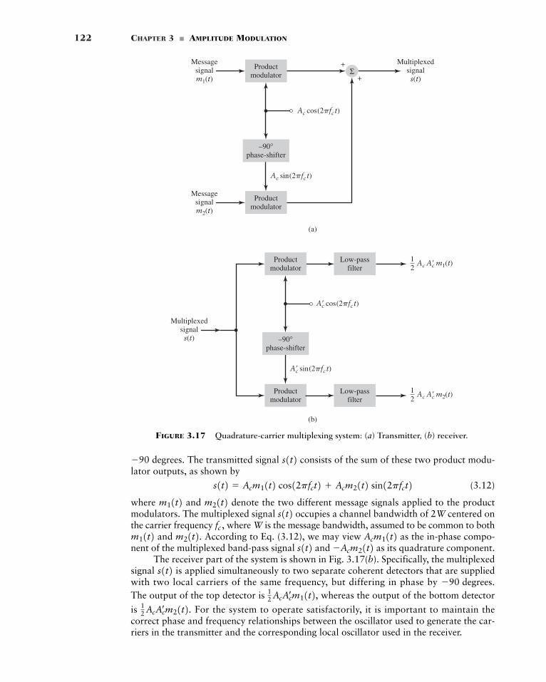
122 CHAPTER 3 � AMPLITUDE MODULATION
(a)
–90°phase-shifter
Multiplexedsignals(t)+
+
Productmodulator
Messagesignalm1(t)
Messagesignalm2(t)
Ac sin(2�fc t)
ΣProductmodulator
Ac cos(2�fc t)
(b)
–90°phase-shifter
Productmodulator
Multiplexedsignals(t)
Ac� sin(2�fc t)
Ac� cos(2�fc t)
Productmodulator
Low-passfilter
Low-passfilter
21 Ac Ac� m1(t)
21 Ac Ac� m2(t)
FIGURE 3.17 Quadrature-carrier multiplexing system: (a) Transmitter, (b) receiver.
The transmitted signal consists of the sum of these two product modu-lator outputs, as shown by
(3.12)
where and denote the two different message signals applied to the productmodulators. The multiplexed signal occupies a channel bandwidth of 2W centered onthe carrier frequency where W is the message bandwidth, assumed to be common to both
and According to Eq. (3.12), we may view as the in-phase compo-nent of the multiplexed band-pass signal and as its quadrature component.
The receiver part of the system is shown in Fig. 3.17(b). Specifically, the multiplexedsignal is applied simultaneously to two separate coherent detectors that are suppliedwith two local carriers of the same frequency, but differing in phase by The output of the top detector is whereas the output of the bottom detector
is For the system to operate satisfactorily, it is important to maintain the correct phase and frequency relationships between the oscillator used to generate the car-riers in the transmitter and the corresponding local oscillator used in the receiver.
12 AcA
œcm21t2.
12 AcA
œcm11t2,
�90 degrees.s1t2
�Acm21t2s1t2 Acm11t2m21t2.m11t2 fc ,s1t2m21t2m11t2
s1t2 � Acm11t2 cos12pfct2 Acm21t2 sin12pfct2s1t2�90 degrees.
3.6 Single-Sidebank Modulation 123
To maintain this synchronization, we may use a Costas receiver described in Section3.4. Another commonly used method is to send a pilot signal outside the passband of themodulated signal. In the latter method, the pilot signal typically consists of a low-powersinusoidal tone whose frequency and phase are related to the carrier wave At the receiver, the pilot signal is extracted by means of a suitably tuned circuit and thentranslated to the correct frequency for use in the coherent detector.
� Drill Problem 3.9 Verify that the outputs of the receiver in Fig. 3.17(b) are as indicatedin the figure, assuming perfect synchronism between the receiver and transmitter. �
3.6 Single-Sideband Modulation
In suppressing the carrier, DSB-SC modulation takes care of a major limitation of AM thatpertains to the wastage of transmitted power. To take care of the other major limitation ofAM that pertains to channel bandwidth, we need to suppress one of the two sidebands inthe DSB-SC modulated wave. This modification of DSB-SC modulation is precisely whatis done in single sideband (SSB) modulation. In effect, SSB modulation relies solely on thelower sideband or upper sideband to transmit the message signal across a communicationchannel. Depending on which particular sideband is actually transmitted, we speak oflower SSB or upper SSB modulation.
� THEORY
A rigorous derivation of SSB modulation theory that applies to an arbitrary message sig-nal is rather demanding and therefore beyond the scope of this book. To simplify matters,we will take an approach different from that used in Section 3.1 on AM and Section 3.3on DSB-SC. Specifically, we start the study of SSB modulation by first considering the sim-ple case of a sinusoidal modulating wave, and then we generalize the results to an arbitrarymodulating signal in a step-by-step manner.
To proceed then, consider a DSB-SC modulator using the sinusoidal modulating wave
With the carrier the resulting DSB-SC modulated wave is defined by
(3.13)
which is characterized by two side-frequencies, one at and the other at Suppose that we would like to generate a sinusoidal SSB modulated wave that retains theupper side-frequency at Then, suppressing the second term in Eq. (3.13), we mayexpress the upper SSB modulated wave as
(3.14)
The cosine term in Eq. (3.14) includes the sum of two angles—namely, and Therefore, expanding the cosine term in Eq. (3.14) using a well-known trigonometricidentity, we have
(3.15)SUSSB1t2 �12
AcAm cos12pfct2 cos12pfmt2 �12
AcAm sin12pfct2 sin12pfmt2
2pfmt.2pfct
SUSSB1t2 �12
AcAm cos32p1fc fm2t4fc fm .
fc � fm .fc fm
�12
AcAm cos32p1fc fm2t4 12
AcAm cos32p1fc � fm2t4� AcAm cos12pfct2 cos12pfmt2
SDSB1t2 � c1t2m1t2c1t2 � Ac cos12pfct2,
m1t2 � Am cos12pfmt2
c1t2 � Ac12pfct2.
124 CHAPTER 3 � AMPLITUDE MODULATION
If, on the other hand, we were to retain the lower side-frequency at in the DSB-SCmodulated wave of Eq. (3.13), then we would have a lower SSB modulated wave defined by
(3.16)
Examining Eqs. (3.15) and (3.16), we see that they differ from each other in only onerespect: the minus sign in Eq. (3.15) is replaced with the plus sign in Eq. (3.16). Accord-ingly, we may combine these two equations and thereby define a sinusoidal SSB modu-lated wave as follows:
(3.17)
where the plus sign applies to lower SSB and the minus sign applies to upper SSB.With the generalization of Eq. (3.17) as the goal, we next proceed in two stages. In
stage 1, we let the message signal be periodic; and in stage 2, we let it be nonperiodic. Con-sider then a periodic message signal defined by the Fourier series
(3.18)
which consists of a mixture of sinusoidal waves with harmonically related frequencies.Recognizing that the carrier is common to all the sinusoidal components of wemay therefore immediately infer from Eq. (3.17) the expression
(3.19)
as the corresponding formula for the SSB modulated wave. Next, let us consider another periodic signal defined by the Fourier series
(3.20)
which is of a form similar to that of Eq. (3.18) except for the fact that the cosine termis replaced by the sine term Then, in light of the definitions in Eqs.
(3.19) and (3.20), we may reformulate the SSB modulated wave of Eq. (3.17) as
(3.21)
Comparing Eq. (3.20) with Eq. (3.18), we observe that the periodic signal can bederived from the periodic modulating signal simply by shifting the phase of eachcosine term in Eq. (3.18) by
In both technical and practical terms, the observation we have just made is veryimportant for two reasons:
1. We know from Fourier analysis that under appropriate conditions, the Fourier seriesrepresentation of a periodic signal converges to the Fourier transform of a nonperi-odic signal; see Appendix 2 for details.
2. The signal is the Hilbert transform of the signal Basically, a Hilbert trans-former is a system whose transfer function is defined by
(3.22)
where sgn(f) is the signum function; for the definition of the signum function seeSection 2.4. In words, the Hilbert transformer is a wide-band phase-shifter whosefrequency response is characterized in two parts as follows (see Problem 2.52):
� The magnitude response is unity for all frequencies, both positive and negative.
H1f2 � �j sgn1f2m1t2.mn 1t2
�90°.m1t2 mn 1t2
SSSB1t2 �Ac
2m1t2 cos12pfct2 <
Ac
2mn 1t2 sin12pfct2
sin12pfct2.cos12pfct2mn 1t2 � a
nan sin12pfnt2
SSSB1t2 �12
Ac cos12pfct2an
an cos12pfnt2 <12
Ac sin12pfct2an
an sin12pfnt2m1t2,c1t2
m1t2 � an
an cos12pfnt2
SSSB1t2 �12
AcAm cos12pfct2 cos12pfmt2 <12
AcAm sin12pfct2 sin12pfmt2
SLSSB1t2 �12
AcAm cos12pfct2 cos12pfmt2 12
AcAm sin12pfct2 sin12pfmt2fc � fm
3.6 Single-Sidebank Modulation 125
� The phase response is for negative frequencies and for positivefrequencies.
Equipped analytically in the manner described under points 1 and 2, we may finally gen-eralize Eq. (3.21) as the formula for a single-sideband modulated wave produced by a mes-sage signal, regardless of whether it is periodic or nonperiodic. Specifically, given a Fouriertransformable message signal with its Hilbert transform denoted by the SSBmodulated wave produced by is defined by
(3.23)
where is the carrier, is its phase-shifted version; the plusand minus signs apply to the lower SSB and upper SSB, respectively. In Eq. (3.23), we haveomitted the use of SSB as a subscript for with it being understood that this equationrefers to SSB modulation in its most generic form.
� Drill Problem 3.10 Using Eqs. (3.22) and (3.23), show that for positive frequencies thespectra of the two kinds of SSB modulated waves are defined as follows:
(a) For the upper SSB,
(3.24)
(b) For the lower SSB,
(3.25)
� Drill Problem 3.11 Show that if the message signal is low-pass, then the Hilberttransform is also low-pass with exactly the same bandwidth as �
The two spectral formulas defined in parts (a) and (b) of Problem 3.10 are intuitivelysatisfying. In particular, they are both in perfect accord with the two pictures displayed inparts (b) and (c) of Fig. 3.18, respectively. Figure 3.18(b) describes an SSB modulated wavethat has retained the upper sideband, whereas Fig. 3.18(c) describes the other kind of SSBmodulation that has retained the lower sideband. From a practical perspective, the only issuethat distinguishes one kind of SSB modulation from the other is that of bandwidthoccupancy.
� MODULATORS FOR SSB
In light of the theory presented in this section, we may develop two methods for generat-ing SSB-modulated waves, as described next.
Frequency Discrimination Method
One straightforward method for SSB generation, called the frequency discriminationmethod, is depicted in Fig. 3.19; this discriminator follows directly from Eqs. (3.24) and(3.25) presented in Problem 3.10. The SSB modulator of Fig. 3.19 consists of two compo-nents: product modulator followed by band-pass filter. The product modulator producesa DSB-SC modulated wave with an upper sideband and a lower sideband. The band-pass
m1t2.mn 1t2 m1t2S1f2 � c 0, for f � fc
Ac
2M1f � fc2, for 0 � f � fc
S1f2 � c Ac
2M1f � fc2, for f � fc
0, for 0 � f � fc
s1t2,�90°Ac sin12pfct2Ac cos12pfct2
s1t2 �Ac
2m1t2 cos12pfct2 <
Ac
2mn 1t2 sin12pfct2
m1t2 mn 1t2,m1t2
�90°90°
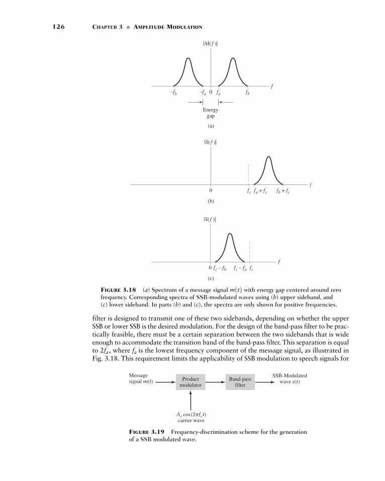
126 CHAPTER 3 � AMPLITUDE MODULATION
f
(a)
–fb –fa
|M( f )|
0
Energygap
fa fb
0f
(b)
|S( f )|
fa + fcfc fb + fc
0f
(c)
|S( f )|
fcfc – fb fc – fa
FIGURE 3.18 (a) Spectrum of a message signal with energy gap centered around zerofrequency. Corresponding spectra of SSB-modulated waves using (b) upper sideband, and(c) lower sideband. In parts (b) and (c), the spectra are only shown for positive frequencies.
m1t2
Ac cos(2�fct)carrier wave
Messagesignal m(t) Product
modulatorBand-pass
filter
SSB-Modulatedwave s(t)
FIGURE 3.19 Frequency-discrimination scheme for the generationof a SSB modulated wave.
filter is designed to transmit one of these two sidebands, depending on whether the upperSSB or lower SSB is the desired modulation. For the design of the band-pass filter to be prac-tically feasible, there must be a certain separation between the two sidebands that is wideenough to accommodate the transition band of the band-pass filter. This separation is equalto where is the lowest frequency component of the message signal, as illustrated inFig. 3.18. This requirement limits the applicability of SSB modulation to speech signals for
fa2fa ,
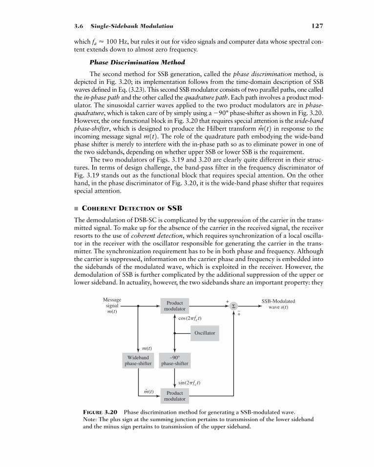
3.6 Single-Sidebank Modulation 127
which but rules it out for video signals and computer data whose spectral con-tent extends down to almost zero frequency.
Phase Discrimination Method
The second method for SSB generation, called the phase discrimination method, isdepicted in Fig. 3.20; its implementation follows from the time-domain description of SSBwaves defined in Eq. (3.23). This second SSB modulator consists of two parallel paths, one calledthe in-phase path and the other called the quadrature path. Each path involves a product mod-ulator. The sinusoidal carrier waves applied to the two product modulators are in phase-quadrature, which is taken care of by simply using a phase-shifter as shown in Fig. 3.20.However, the one functional block in Fig. 3.20 that requires special attention is the wide-bandphase-shifter, which is designed to produce the Hilbert transform in response to theincoming message signal The role of the quadrature path embodying the wide-bandphase shifter is merely to interfere with the in-phase path so as to eliminate power in one ofthe two sidebands, depending on whether upper SSB or lower SSB is the requirement.
The two modulators of Figs. 3.19 and 3.20 are clearly quite different in their struc-tures. In terms of design challenge, the band-pass filter in the frequency discriminator ofFig. 3.19 stands out as the functional block that requires special attention. On the otherhand, in the phase discriminator of Fig. 3.20, it is the wide-band phase shifter that requiresspecial attention.
� COHERENT DETECTION OF SSB
The demodulation of DSB-SC is complicated by the suppression of the carrier in the trans-mitted signal. To make up for the absence of the carrier in the received signal, the receiverresorts to the use of coherent detection, which requires synchronization of a local oscilla-tor in the receiver with the oscillator responsible for generating the carrier in the trans-mitter. The synchronization requirement has to be in both phase and frequency. Althoughthe carrier is suppressed, information on the carrier phase and frequency is embedded intothe sidebands of the modulated wave, which is exploited in the receiver. However, thedemodulation of SSB is further complicated by the additional suppression of the upper orlower sideband. In actuality, however, the two sidebands share an important property: they
m1t2. mn 1t2�90°
fa � 100 Hz,
–90°phase-shifter
Widebandphase-shifter
SSB-Modulatedwave s(t)
–+
+
Productmodulator
Messagesignalm(t)
m(t)ˆ
m(t)
cos(2�fc t)
sin(2�fc t)
ΣProductmodulator
Oscillator
FIGURE 3.20 Phase discrimination method for generating a SSB-modulated wave.Note: The plus sign at the summing junction pertains to transmission of the lower sidebandand the minus sign pertains to transmission of the upper sideband.
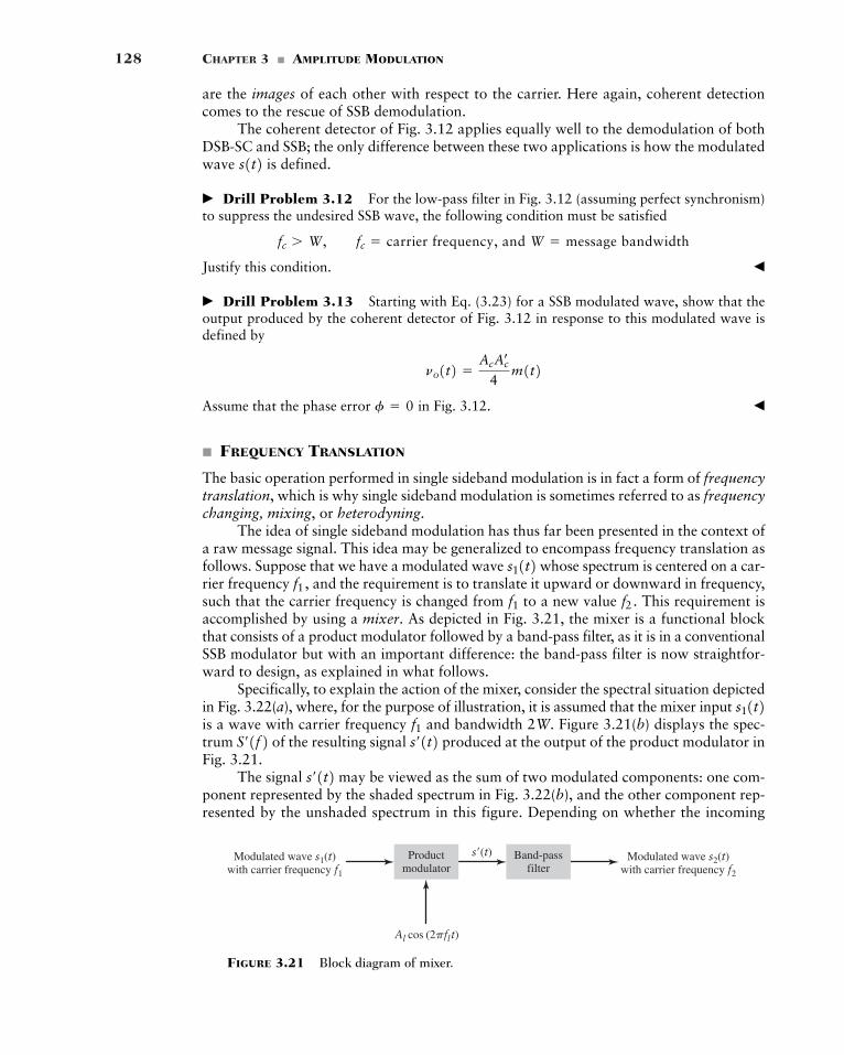
128 CHAPTER 3 � AMPLITUDE MODULATION
are the images of each other with respect to the carrier. Here again, coherent detectioncomes to the rescue of SSB demodulation.
The coherent detector of Fig. 3.12 applies equally well to the demodulation of bothDSB-SC and SSB; the only difference between these two applications is how the modulatedwave is defined.
� Drill Problem 3.12 For the low-pass filter in Fig. 3.12 (assuming perfect synchronism)to suppress the undesired SSB wave, the following condition must be satisfied
Justify this condition. �
� Drill Problem 3.13 Starting with Eq. (3.23) for a SSB modulated wave, show that theoutput produced by the coherent detector of Fig. 3.12 in response to this modulated wave isdefined by
Assume that the phase error in Fig. 3.12. �
� FREQUENCY TRANSLATION
The basic operation performed in single sideband modulation is in fact a form of frequencytranslation, which is why single sideband modulation is sometimes referred to as frequencychanging, mixing, or heterodyning.
The idea of single sideband modulation has thus far been presented in the context ofa raw message signal. This idea may be generalized to encompass frequency translation asfollows. Suppose that we have a modulated wave whose spectrum is centered on a car-rier frequency and the requirement is to translate it upward or downward in frequency,such that the carrier frequency is changed from to a new value This requirement isaccomplished by using a mixer. As depicted in Fig. 3.21, the mixer is a functional blockthat consists of a product modulator followed by a band-pass filter, as it is in a conventionalSSB modulator but with an important difference: the band-pass filter is now straightfor-ward to design, as explained in what follows.
Specifically, to explain the action of the mixer, consider the spectral situation depictedin Fig. 3.22(a), where, for the purpose of illustration, it is assumed that the mixer input is a wave with carrier frequency and bandwidth 2W. Figure 3.21(b) displays the spec-trum of the resulting signal produced at the output of the product modulator inFig. 3.21.
The signal may be viewed as the sum of two modulated components: one com-ponent represented by the shaded spectrum in Fig. 3.22(b), and the other component rep-resented by the unshaded spectrum in this figure. Depending on whether the incoming
s�1t2s�1t2S�1f2 f1
s11t2
f2.f1f1,
s11t2
f � 0
no1t2 �AcA
œc
4m1t2
fc � W, fc � carrier frequency, and W � message bandwidth
s1t2
Modulated wave s1(t)with carrier frequency f1
s�(t) Modulated wave s2(t)with carrier frequency f2
Al cos (2�flt)
Productmodulator
Band-passfilter
FIGURE 3.21 Block diagram of mixer.
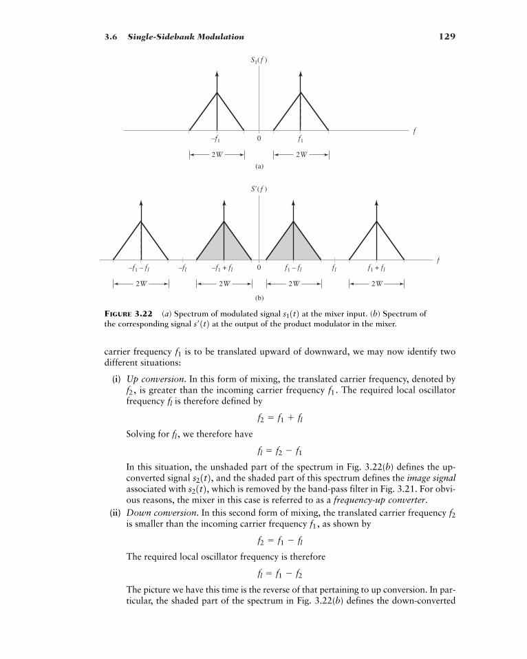
3.6 Single-Sidebank Modulation 129
S�( f )
f0
(b)
–f1 – fl
2W
–f1 + fl fl –fl f1 – fl f1 + fl
2W 2W 2W
S1( f )
f0
(a)
–f1 f1
2W 2W
FIGURE 3.22 (a) Spectrum of modulated signal at the mixer input. (b) Spectrum ofthe corresponding signal at the output of the product modulator in the mixer.s�1t2 s11t2
carrier frequency is to be translated upward of downward, we may now identify twodifferent situations:
(i) Up conversion. In this form of mixing, the translated carrier frequency, denoted byis greater than the incoming carrier frequency The required local oscillator
frequency is therefore defined by
Solving for we therefore have
In this situation, the unshaded part of the spectrum in Fig. 3.22(b) defines the up-converted signal and the shaded part of this spectrum defines the image signalassociated with which is removed by the band-pass filter in Fig. 3.21. For obvi-ous reasons, the mixer in this case is referred to as a frequency-up converter.
(ii) Down conversion. In this second form of mixing, the translated carrier frequency is smaller than the incoming carrier frequency as shown by
The required local oscillator frequency is therefore
The picture we have this time is the reverse of that pertaining to up conversion. In par-ticular, the shaded part of the spectrum in Fig. 3.22(b) defines the down-converted
fl � f1 � f2
f2 � f1 � fl
f1,f2
s21t2,s21t2,fl � f2 � f1
fl ,
f2 � f1 fl
flf1.f2,
f1

130 CHAPTER 3 � AMPLITUDE MODULATION
signal and the unshaded part of this spectrum defines the associated image sig-nal. Accordingly, this second mixer is referred to as a frequency-down converter. Notethat in this case, the translated carrier frequency has to be larger than W (i.e., one halfof the bandwidth of the incoming modulated signal ) to avoid sideband overlap.
The purpose of the band-pass filter in the mixer of Fig. 3.21 is now clear: pass the sig-nal and eliminate the associated image signal. This objective is achieved by aligningthe midband frequency of the filter with the translated carrier frequency and assigningit a bandwidth equal to that of the incoming modulated signal Regardless of whetherthe frequency conversion is up or down, the transition band of the filter is permitted tooccupy the gap from to that is, the permissible width of the tran-sition band is which, in effect, requires that the local oscillator frequency begreater than W. Moreover, to avoid spectoral overlap in down conversion, we also requirethat be greater than zero; that is,
It is important to note that mixing is a linear operation. Accordingly, the relation ofthe sidebands of the incoming modulated wave to the original carrier existing at the mixerinput is completely preserved at the mixer output.
3.7 Vestigial Sideband Modulation
� MOTIVATION
Single-sideband modulation works satisfactorily for an information-bearing signal (e.g.,speech signal) with an energy gap centered around zero frequency. However, for the spec-trally efficient transmission of wideband signals, we have to look to a new method of mod-ulation for two reasons:
1. Typically, the spectra of wideband signals (exemplified by television video signals andcomputer data) contain significant low frequencies, which make it impractical to useSSB modulation.
2. The spectral characteristics of wideband data befit the use of DSB-SC. However, DSB-SC requires a transmission bandwidth equal to twice the message bandwidth, whichviolates the bandwidth conservation requirement.
To overcome these two practical limitations, we need a compromise method of modulationthat lies somewhere between SSB and DSB-SC in its spectral characteristics. Vestigial side-band, the remaining modulation scheme to be considered in this section, is that compro-mise scheme.
Vestigial sideband (VSB) modulation distinguishes itself from SSB modulation in twopractical respects:
1. Instead of completely removing a sideband, a trace or vestige of that sideband istransmitted; hence, the name “vestigial sideband.”
2. Instead of transmitting the other sideband in full, almost the whole of this second bandis also transmitted.
Accordingly, the transmission bandwidth of a VSB modulated signal is defined by
where is the vestige bandwidth and W is the message bandwidth. Typically, is 25percent of W, which means that the VSB bandwidth lies between the SSB bandwidth,W, and DSB-SC bandwidth, 2W.
BT
fnfn
BT � fn W
fl � f1 � W.f1 � fl � W
fl21fl � W2, f1 fl � W;f1 � fl W
s11t2. f2s21t2
s21t2f2
s21t2,
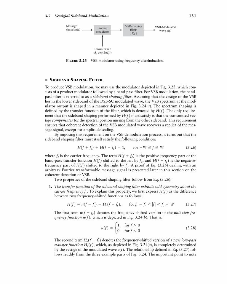
3.7 Vestigial Sideband Modulation 131
� SIDEBAND SHAPING FILTER
To produce VSB modulation, we may use the modulator depicted in Fig. 3.23, which con-sists of a product modulator followed by a band-pass filter. For VSB modulation, the band-pass filter is referred to as a sideband shaping filter. Assuming that the vestige of the VSBlies in the lower sideband of the DSB-SC modulated wave, the VSB spectrum at the mod-ulator output is shaped in a manner depicted in Fig. 3.24(a). The spectrum shaping isdefined by the transfer function of the filter, which is denoted by The only require-ment that the sideband shaping performed by must satisfy is that the transmitted ves-tige compensates for the spectral portion missing from the other sideband. This requirementensures that coherent detection of the VSB modulated wave recovers a replica of the mes-sage signal, except for amplitude scaling.
By imposing this requirement on the VSB demodulation process, it turns out that thesideband shaping filter must itself satisfy the following condition:
(3.26)
where is the carrier frequency. The term is the positive-frequency part of theband-pass transfer function shifted to the left by and is the negative-frequency part of shifted to the right by A proof of Eq. (3.26) dealing with anarbitrary Fourier transformable message signal is presented later in this section on thecoherent detection of VSB.
Two properties of the sideband shaping filter follow from Eq. (3.26):
1. The transfer function of the sideband shaping filter exhibits odd symmetry about thecarrier frequency To explain this property, we first express as the differencebetween two frequency-shifted functions as follows:
(3.27)
The first term denotes the frequency-shifted version of the unit-step fre-quency function which is depicted in Fig. 3.24(b). That is,
(3.28)
The second term denotes the frequency-shifted version of a new low-passtransfer function which, as depicted in Fig. 3.24(c), is completely determinedby the vestige of the modulated wave The relationship defined in Eq. (3.27) fol-lows readily from the three example parts of Fig. 3.24. The important point to note
s1t2.Hn1f2,Hn1f � fc2u1f2 � b1, for f � 0
0, for f � 0
u1f2,u1f � fc2H1f2 � u1f � fc2 � Hn1f � fc2, for fc � fn � ƒf ƒ � fc W
H1f2fc .
fc .H1f2 H1f � fc2fc ,H1f2 H1f fc2fc
H1f fc2 H1f � fc2 � 1, for �W � f � W
H1f2 H1f2.
Carrier waveAc cos(2�fct)
Messagesignal m(t) Product
modulator
VSB-shapingfilter:H(f )
VSB-Modulatedwave s(t)
FIGURE 3.23 VSB modulator using frequency discrimination.
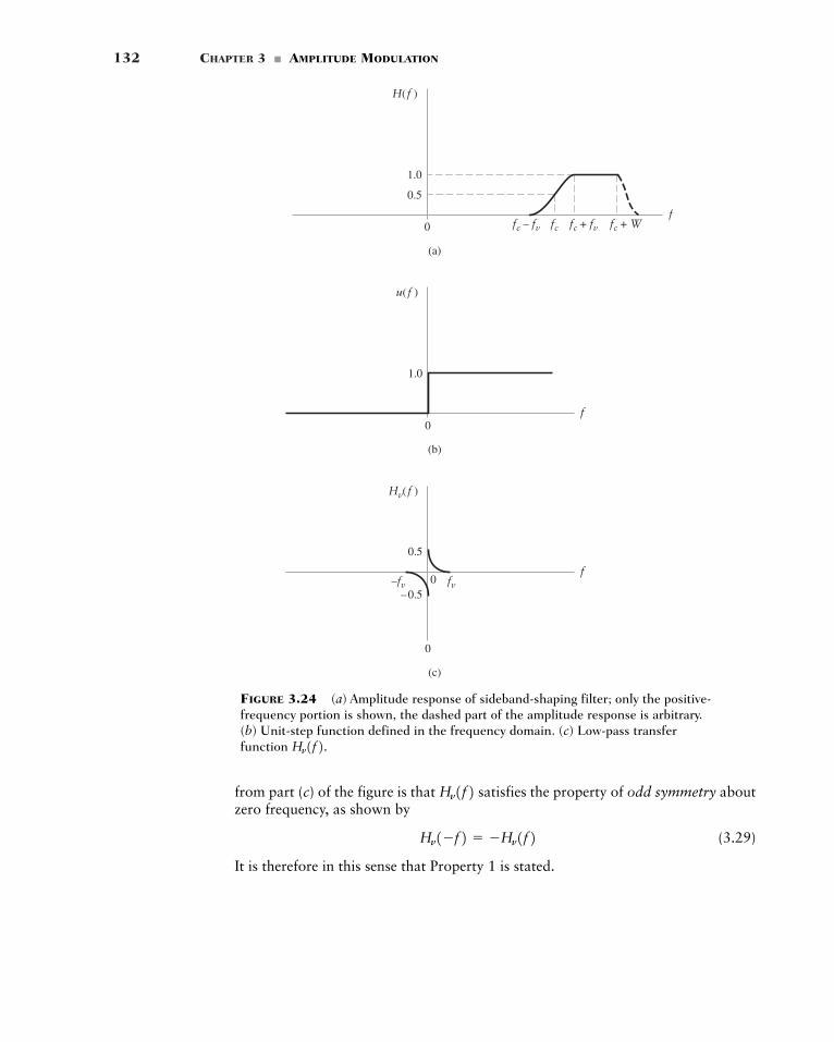
132 CHAPTER 3 � AMPLITUDE MODULATION
(b)
u( f )
f0
1.0
(a)
H( f )
f0
1.0
0.5
fc – fv fc + fv fc + Wfc
(c)
fv–fv
Hv( f )
f
0
0.5
–0.50
FIGURE 3.24 (a) Amplitude response of sideband-shaping filter; only the positive-frequency portion is shown, the dashed part of the amplitude response is arbitrary.(b) Unit-step function defined in the frequency domain. (c) Low-pass transferfunction Hn1f2.
from part (c) of the figure is that satisfies the property of odd symmetry aboutzero frequency, as shown by
(3.29)
It is therefore in this sense that Property 1 is stated.
Hn1�f2 � �Hn1f2Hn1f2
3.7 Vestigial Sideband Modulation 133
2. The transfer function is required to satisfy the condition of Eq. (3.26) only forthe frequency interval where W is the message bandwidth. The prac-tical implication of this second property is that, for the case of VSB depicted in Fig. 3.24(a), the transfer function of the sideband shaping filter can have an arbi-trary specification for it is for this reason that the part of the spectrumlying above is shown dashed in Fig. 3.24(a).
EXAMPLE 3.3 Sinusoidal VSB
Consider the simple example of sinusoidal VSB modulation produced by the sinusoidal mod-ulating wave
and carrier wave
Let the upper side-frequency at as well as its image at be attenuated by thefactor k. To satisfy the condition of Eq. (3.26), the lower side-frequency at and itsimage must be attenuated by the factor The VSB spectrum is therefore
Correspondingly, the sinusoidal VSB modulated wave is defined by
(3.30)
Using well-known trigonometric identities to expand the cosine terms andwe may reformulate Eq. (3.30) as the linear combination of two sinusoidal
DSB-SC modulated waves.
(3.31)
where the first term on the right-hand side is the in-phase component of and the secondterm is the quadrature component.
s1t2
12
AcAm11 � 2k2 sin112pfct2 sin12pfmt22s1t2 �
12
AcAm cos12pfct2 cos12pfmt2
cos12p1fc � fm2t2, cos12p1fc fm2t2�
12
kAcAm cos12p1fc fm2t2 1211 � k2AcAm cos12p1fc � fm2t2
1411 � k2AcAm3exp1j2p1fc � fm2t2 exp1�j2p1fc � fm2t24
s1t2 �14
kAcAm3exp1j2p1fc fm2t2 exp1�j2p1fc fm2t24
1411 � k2AcAm3d1f � 1fc � fm22 d1f 1fc � fm224
S1f2 �14
kAcAm3d1f � 1fc fm22 d1f 1fc fm22411 � k2.�1fc � fm2 fc � fm
�1fc fm2fc fm
c1t2 � Ac cos12pfct2
m1t2 � Am cos12pfmt2
fc Wƒf ƒ � fc W;
�W � f � W,Hn1f2
134 CHAPTER 3 � AMPLITUDE MODULATION
To summarize, depending on how the attenuation factor k in Eq. (3.31) is defined inthe interval (0, 1), we may identify all the different sinusoidal forms of linear modulatedwaves studied in Sections 3.3, 3.6, and 3.7 as follows:
1. for which reduces to DSB-SC
2. for which reduces to lower SSBfor which reduces to upper SSB
3. for which the attenuated version of the upper side-frequency defines the
vestige of
for which the attenuated version of the lower side frequency defines the
vestige of
� COHERENT DETECTION OF VSB
For an exact recovery of the message signal from the VSB modulated wave exceptfor some amplitude scaling, we may use the coherent detector shown in Fig. 3.12. As withthe DSB-SC and SSB demodulations studied previously, the demodulation of VSB consistsof multiplying with a locally generated sinusoid and then low-pass filtering the result-ing product signal It is assumed that the local sinusoid in the coherent detector ofFig. 3.12 is in perfect synchronism with the carrier in the modulator responsible for gen-erating the VSB-modulated wave. Then setting the phase in the local sinusoid in Fig. 3.12equal to zero, we express the Fourier transform of the product signal
as follows
(3.32)
where
Next, we express the Fourier transform of the VSB modulated wave as
(3.33)
which follows from Fig. 3.23 depicting the VSB modulator; M(f) is the message spectrumand is the transfer function of the sideband shaping filter. Shifting the VSB spectrum
to the right by yields
(3.34)
and shifting it to the left by yields
(3.35)S1f fc2 �12
Ac3M1f2 M1f 2fc24H1f fc2fc
S1f � fc2 �12
Ac3M1f � 2fc2 M1f24H1f � fc2fcS1f2H1f2
S1f2 �12
Ac3M1f � fc2 M1f fc24H1f2s1t2
s1t2 Δ S1f2
V1f2 �12
Acœ3S1f � fc2 S1f fc24
n1t2 � Acœs1t2 cos12pfct2
f
n1t2.s1t2s1t2,m1t2
s1t212
� k � 1,
s1t20 � k �
12
,
s1t2k � 1,s1t2k � 0,
s1t2k �12
,
3.7 Vestigial Sideband Modulation 135
Hence, substituting Eqs. (3.34) and (3.35) into Eq. (3.32) and then combining terms, weobtain
which, in light of the condition imposed on in Eq. (3.26), reduces to
(3.36)
The first term on the right-hand side of Eq. (3.36) is a scaled version of the message spec-trum The second term of Eq. (3.36) is the Fourier transform of high-frequency com-ponents, representing a new VSB wave modulated onto a carrier of frequency Providedthat the low-pass filter in the coherent detector of Fig. 3.12 has a cutoff frequency justslightly greater than the message bandwidth, the high-frequency components of areremoved by the low-pass filter. The resulting demodulated signal is a scaled version of thedesired message signal
� Drill Problem 3.14 Validate the statement that the high-frequency components in Eq. (3.36) represent a VSB wave modulated onto a carrier of frequency �
EXAMPLE 3.4 Coherent detection of sinusoidal VSB
Recall from Eq. (3.31) of Example 3.3, that the sinusoidal VSB modulated signal is defined by
Multiplying by in accordance with perfect coherent detection yields theproduct signal
Next, using the trigonometric identities
cos212pfct2 �1231 cos14pfct24
12
AcAcœAm11 � 2k2 sin12pfmt2 sin12pfct2 cos12pfct2
�12
AcAcœAm cos12pfmt2 cos212pfct2
n1t2 � Acœs1t2 cos12pfct2
Acœ cos12pfct2s1t2
12
AcAm11 � 2k2 sin12pfct2 sin12pfmt2s1t2 �
12
AcAm cos12pfmt2 cos12pfct2
2fc .
m1t2.n1t2
2fc .M1f2.
14
AcAcœ3M1f � 2fc2H1f � fc2 M1f 2fc2H1f fc24
V1f2 �14
AcAcœM1f2
H1f2
14
AcAcœ3M1f � 2fc2H1f � fc2 M1f 2fc2H1f fc24
V1f2 �14
AcAcœM1f23H1f � fc2 H1f fc24
136 CHAPTER 3 � AMPLITUDE MODULATION
3 Another procedure used for the detection of a VSB modulated wave is to add a pilot to the modulated wave atthe transmitter. The pilot would be a frequency-translated version of the carrier used in the generation of themodulated wave, but it lies outside the band of frequencies occupied by the modulated wave. At the receiver, thepilot is extracted by means of a band-pass filter and then translated (upward or downward) to produce a replicaof the original carrier. With this replica of the carrier available to the receiver, coherent detection may be used torecover the original message signal.
A similar procedure can be used for the coherent detection of SSB modulated waves.
and
we may redefine as
(3.37)
The first term on the right-hand side of Eq. (3.37) is a scaled version of the message signalThe second term of the equation is a new sinusoidal VSB wave modulated
onto a carrier of frequency which represents the high-frequency components of Thissecond term is removed by the low-pass filter in the detector of Fig. 3.12, provided that the cut-off frequency of the filter is just slightly greater than the message frequency
EXAMPLE 3.5 Envelope detection of VSB plus carrier
The coherent detection of VSB requires synchronism of the receiver to the transmitter, whichincreases system complexity. To simplify the demodulation process, we may purposely add thecarrier to the VSB signal (scaled by the factor ) prior to transmission and then use envelopedetection in the receiver.3 Assuming sinusoidal modulation, the “VSB-plus-carrier” signal isdefined [see Eq. (3.31) of Example 3.3) as
The envelope of is therefore
(3.38)� AcB1 ka
2Am cos12pfmt2R d 1 D ka
2Am11 � 2k2 sin12pfmt21
ka
2Am cos12pfmt2 T2 t1>2
a1t2 � bAc2B1
ka
2Am cos12pfmt2R2
Ac2Bka
2Am11 � 2k2 sin12pfmt2R2 r1>2
sVSBC1t2
ka
2AcAm11 � 2k2 sin12pfmt2 sin12pfct2
� AcB1 ka
2Am cos12pfmt2R cos12pfct2
ka
2AcAm11 � 2k2 sin12pfmt2 sin12pfct2
� Ac cos12pfct2 ka
2AcAm cos12pfmt2 cos12pfct2
sVSBC1t2 � Ac cos12pfct2 kas1t2, ka � amplitude sensitivity factor
ka
fm .
n1t2.2fc ,Am cos12pfmt2.
14
AcAcœAm3cos12pfmt2 cos14pfct2 11 � 2k2 sin12pfmt2 sin14pfct24
n1t2 �14
AcAcœAm cos12pfmt2
n1t2sin12pfct2 cos12pfct2 �
12
sin14pfct2
3.8 Baseband Representation of Modulated Waves and Band-Pass Filters 137
Equation (3.38) shows that distortion in the envelope detection performed on the envelopeis contributed by the quadrature component of the sinusoidal VSB signal. This distortion
can be reduced by using a combination of two methods:
� The amplitude sensitivity factor is reduced, which has the effect of reducing the per-centage modulation.
� The width of the vestigial sideband is reduced, which has the effect of reducing the fac-tor
Both of these methods are intuitively satisfying in light of what we see inside the square brack-ets in Eq. (3.38).
3.8 Baseband Representation of ModulatedWaves and Band-Pass Filters
From the discussion of different modulation strategies presented in this chapter, we seethat a modulated wave using a sinusoidal wave as the carrier is actually a band-pass sig-nal centered on the carrier frequency. By virtue of this very fact, the carrier wave imprintsitself into the structure of the modulated wave. In an explicit sense, it does so when the car-rier wave is contained as a separate component in the transmitted signal. When the carrierwave is suppressed, it makes its presence known to the receiver in an implicit sense by posi-tioning the sidebands of the transmitted spectrum around the carrier frequency in one formor another, depending on the type of modulation used.
Typically, the carrier frequency is large compared to the message bandwidth, whichmakes the processing of a modulated wave on a digital computer a difficult proposition.However, from the modulation theory presented in this chapter, we do know that all theinformation content of a message signal resides completely in the sidebands of the modu-lated wave. Accordingly, when the objective is to process a modulated wave on a com-puter, the efficient procedure is to do the processing on the baseband version of themodulated wave rather than directly on the modulated wave itself. The term “baseband”is used to designate the band of frequencies representing the original signal as delivered bya source of information.
� BASEBAND REPRESENTATION OF MODULATED WAVES
Consider then a generic, linear modulated wave, which is defined by
(3.39)
Let
be the carrier wave with frequency and
be the quadrature-phase version of the carrier. To simplify matters, without loss of gener-ality we have set the carrier amplitude equal to unity. We now express the modulated wavein the compact form
(3.40)s1t2 � sI1t2c1t2 � sQ1t2cn1t2
cn1t2 � sin12pfct2fc ,
c1t2 � cos12pfct2s1t2 � sI1t2 cos12pfct2 � sQ1t2 sin12pfct2
11 � 2k2.
ka
a1t2
138 CHAPTER 3 � AMPLITUDE MODULATION
The term is called the in-phase component of the modulated wave so calledbecause it is multiplied by the carrier By the same token, the term is called thequadrature-phase component or simply the quadrature component of so called becauseit is multiplied by the quadrature carrier The carriers and are orthogonal toeach other.
Equation (3.39) or (3.40) is itself referred to as the canonical representation of lin-ear modulated waves. Most important, this representation includes all the members of theamplitude modulation family discussed in this chapter, as shown in Table 3.1.
From this table, it is clearly apparent that the information content of the messagesignal and the way in which the modulation strategy is implemented are fully describedby the in-phase component in both AM and DSB-SC, or in the combination of the in-phase component and the quadrature component in both SSB and VSB. More-over, the orthogonality of and with respect to each other prompts us to introducea new signal called the complex envelope of the modulated wave which is formallydefined by
(3.41)
This definition is motivated by the way in which we deal with complex numbers. In anyevent, the important point to take from Eq. (3.41) is the fact that the complex envelope accounts fully for the information contents of both and Note, however, that thecomplex envelope is a fictitious signal, the use of which is intended merely to simplifysignal processing operations on band-pass signals, which are exemplified by modulatedwaves based on a sinusoidal carrier.
In a manner corresponding to Eq. (3.41), we may define the complex carrier wave
(3.42)
Accordingly, the modulated wave is itself defined by
(3.43)
where extracts the real part of the complex quantity enclosed inside the squarebrackets.
Now we can see the practical advantage of the complex envelope over the real-valued modulated wave
1. The highest frequency component of may be as large as where is thecarrier frequency and W is the message bandwidth.
2. On the other hand, the highest frequency component of is considerably smaller,being limited by the message bandwidth W.
Yet, in using Eq. (3.43) as the representation of the modulated wave there is nothinglost whatsoever.
Given an arbitrary modulated wave we may derive the in-phase compound and quadrature component using the scheme shown in Fig. 3.25(a). Conversely, givensQ1t2 sI1t2s1t2,
s1t2,s'1t2
fcfc W,s1t2s1t2: s
'1t2Re3 # 4
� Re3s'1t2 exp1j2pfct24s1t2 � Re3s'1t2c'1t24
s1t2� exp1j2pfct2� cos12pfct2 j sin12pfct2
c'1t2 � c1t2 jcn1t2
s'1t2 sQ1t2.sI1t2 s
'1t2s'1t2 � sI1t2 jsQ1t2
s1t2,sQ1t2sI1t2 sQ1t2sI1t2 sI1t2m1t2
cn1t2c1t2cn1t2. s1t2,sQ1t2c1t2. s1t2,sI1t2
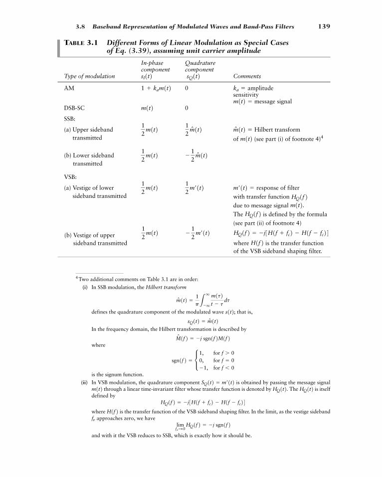
3.8 Baseband Representation of Modulated Waves and Band-Pass Filters 139
4 Two additional comments on Table 3.1 are in order:
(i) In SSB modulation, the Hilbert transform
defines the quadrature component of the modulated wave that is,
In the frequency domain, the Hilbert transformation is described by
where
is the signum function.
(ii) In VSB modulation, the quadrature component is obtained by passing the message signalthrough a linear time-invariant filter whose transfer function is denoted by The is itself
defined by
where is the transfer function of the VSB sideband shaping filter. In the limit, as the vestige sidebandapproaches zero, we have
and with it the VSB reduces to SSB, which is exactly how it should be.
limfnS0
HQ1f2 � �j sgn1f2fn
H1f2HQ1f2 � �j3H1f fc2 � H1f � fc24
HQ1t2HQ1t2.m1t2 SQ1t2 � m�1t2
sgn1f2 � c 1, for f � 00, for f � 0�1, for f � 0
Mn 1f2 � �j sgn1f2M1f2sQ1t2 � mn 1t2
s1t2;mn 1t2 �
1pL
q
�q
m1t2t � t
dt
(b) Vestige of upper sideband transmitted where is the transfer function
of the VSB sideband shaping filter.H1f2
HQ1f2 � �j3H1f fc2 � H1f � fc24�12
m�1t212
m1t2
TABLE 3.1 Different Forms of Linear Modulation as Special Cases of Eq. (3.39), assuming unit carrier amplitude
In-phase Quadraturecomponent component
Type of modulation Comments
AM 0sensitivity
signalDSB-SC 0
SSB:
(a) Upper sideband transform transmitted of (see part (i) of footnote 4)4
(b) Lower sideband transmitted
VSB:
(a) Vestige of lower of filter sideband transmitted with transfer function
due to message signal
The is defined by the formula
(see part (ii) of footnote 4)
HQ1f2m1t2.HQ1f2
m�1t2 � response12
m�1t212
m1t2
�12
mn 1t212
m1t2m1t2
mn 1t2 � Hilbert12
mn 1t212
m1t2m1t2 m1t2 � message
ka � amplitude1 kam1t2sQ1t2sI1t2
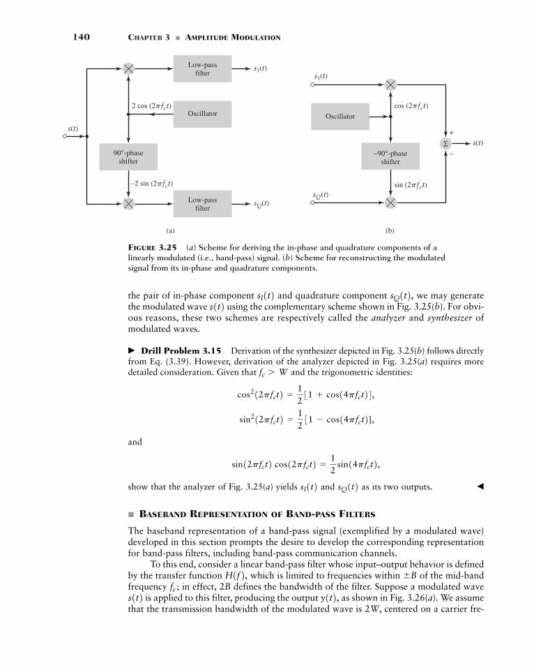
140 CHAPTER 3 � AMPLITUDE MODULATION
Σ
s1(t)Low-passfilter
(a) (b)
Oscillator
–90°-phaseshifter
2 cos (2�fct)
s(t)
s1(t)
s(t)
sQ(t)
–2 sin (2�fct) sin (2�fct)
cos (2�fct)
+
–
sQ(t)Low-passfilter
90°-phaseshifter
Oscillator
FIGURE 3.25 (a) Scheme for deriving the in-phase and quadrature components of alinearly modulated (i.e., band-pass) signal. (b) Scheme for reconstructing the modulatedsignal from its in-phase and quadrature components.
the pair of in-phase component and quadrature component we may generatethe modulated wave using the complementary scheme shown in Fig. 3.25(b). For obvi-ous reasons, these two schemes are respectively called the analyzer and synthesizer ofmodulated waves.
� Drill Problem 3.15 Derivation of the synthesizer depicted in Fig. 3.25(b) follows directlyfrom Eq. (3.39). However, derivation of the analyzer depicted in Fig. 3.25(a) requires moredetailed consideration. Given that and the trigonometric identities:
and
show that the analyzer of Fig. 3.25(a) yields and as its two outputs. �
� BASEBAND REPRESENTATION OF BAND-PASS FILTERS
The baseband representation of a band-pass signal (exemplified by a modulated wave)developed in this section prompts the desire to develop the corresponding representationfor band-pass filters, including band-pass communication channels.
To this end, consider a linear band-pass filter whose input–output behavior is definedby the transfer function which is limited to frequencies within of the mid-bandfrequency in effect, 2B defines the bandwidth of the filter. Suppose a modulated wave
is applied to this filter, producing the output as shown in Fig. 3.26(a). We assumethat the transmission bandwidth of the modulated wave is 2W, centered on a carrier fre-
y1t2,s1t2 fc ;�BH1f2,
sQ1t2sI1t2sin12pfct2 cos12pfct2 �
12
sin14pfct2,
sin212pfct2 �1231 � cos14pfct2],
cos212pfct2 �1231 cos14pfct24,
fc � W
s1t2 sQ1t2,sI1t2
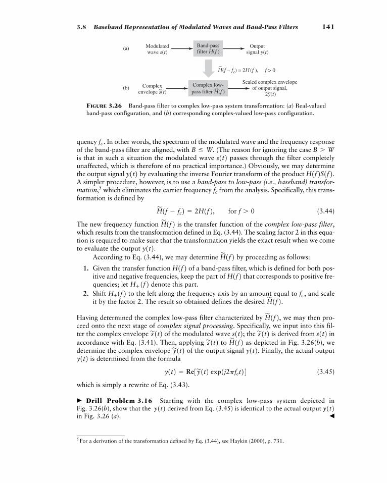
3.8 Baseband Representation of Modulated Waves and Band-Pass Filters 141
(a)
(b)
Modulatedwave s(t)
Outputsignal y(t)
Band-passfilter H(f )
Complexenvelope s(t)
Scaled complex envelopeof output signal,
2y(t)
H(f – fc) = 2H (f ), f > 0~
~~Complex low-pass filter H(f )
~
FIGURE 3.26 Band-pass filter to complex low-pass system transformation: (a) Real-valuedband-pass configuration, and (b) corresponding complex-valued low-pass configuration.
5 For a derivation of the transformation defined by Eq. (3.44), see Haykin (2000), p. 731.
quency In other words, the spectrum of the modulated wave and the frequency responseof the band-pass filter are aligned, with (The reason for ignoring the case is that in such a situation the modulated wave passes through the filter completelyunaffected, which is therefore of no practical importance.) Obviously, we may determinethe output signal by evaluating the inverse Fourier transform of the product A simpler procedure, however, is to use a band-pass to low-pass (i.e., baseband) transfor-mation,5 which eliminates the carrier frequency from the analysis. Specifically, this trans-formation is defined by
(3.44)
The new frequency function is the transfer function of the complex low-pass filter,which results from the transformation defined in Eq. (3.44). The scaling factor 2 in this equa-tion is required to make sure that the transformation yields the exact result when we cometo evaluate the output
According to Eq. (3.44), we may determine by proceeding as follows:
1. Given the transfer function of a band-pass filter, which is defined for both pos-itive and negative frequencies, keep the part of that corresponds to positive fre-quencies; let denote this part.
2. Shift to the left along the frequency axis by an amount equal to and scaleit by the factor 2. The result so obtained defines the desired
Having determined the complex low-pass filter characterized by we may then pro-ceed onto the next stage of complex signal processing. Specifically, we input into this fil-ter the complex envelope of the modulated wave the is derived from in accordance with Eq. (3.41). Then, applying to as depicted in Fig. 3.26(b), wedetermine the complex envelope of the output signal Finally, the actual output
is determined from the formula
(3.45)
which is simply a rewrite of Eq. (3.43).
� Drill Problem 3.16 Starting with the complex low-pass system depicted inFig. 3.26(b), show that the derived from Eq. (3.45) is identical to the actual output in Fig. 3.26 (a). �
y1t2y1t2
y1t2 � Re3y'1t2 exp1j2pfct24y1t2 y1t2.y
'1t2 H'1f2s
'1t2 s1t2s'1t2s1t2;s
'1t2H'1f2,H'1f2. fc ,H1f2
H1f2 H1f2H1f2H'1f2y1t2.
H'1f2
H'1f � fc2 � 2H1f2, for f � 0
fc
H1f2S1f2.y1t2s1t2 B � WB � W.
fc .
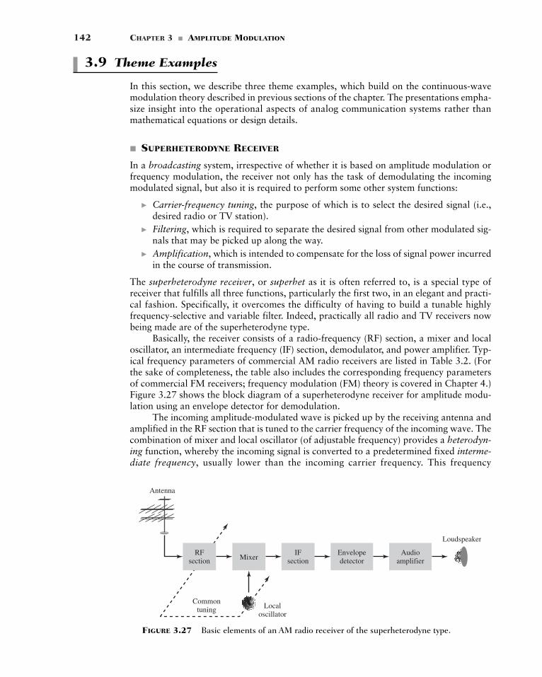
142 CHAPTER 3 � AMPLITUDE MODULATION
3.9 Theme Examples
In this section, we describe three theme examples, which build on the continuous-wavemodulation theory described in previous sections of the chapter. The presentations empha-size insight into the operational aspects of analog communication systems rather thanmathematical equations or design details.
� SUPERHETERODYNE RECEIVER
In a broadcasting system, irrespective of whether it is based on amplitude modulation orfrequency modulation, the receiver not only has the task of demodulating the incomingmodulated signal, but also it is required to perform some other system functions:
� Carrier-frequency tuning, the purpose of which is to select the desired signal (i.e.,desired radio or TV station).
� Filtering, which is required to separate the desired signal from other modulated sig-nals that may be picked up along the way.
� Amplification, which is intended to compensate for the loss of signal power incurredin the course of transmission.
The superheterodyne receiver, or superhet as it is often referred to, is a special type ofreceiver that fulfills all three functions, particularly the first two, in an elegant and practi-cal fashion. Specifically, it overcomes the difficulty of having to build a tunable highlyfrequency-selective and variable filter. Indeed, practically all radio and TV receivers nowbeing made are of the superheterodyne type.
Basically, the receiver consists of a radio-frequency (RF) section, a mixer and localoscillator, an intermediate frequency (IF) section, demodulator, and power amplifier. Typ-ical frequency parameters of commercial AM radio receivers are listed in Table 3.2. (Forthe sake of completeness, the table also includes the corresponding frequency parametersof commercial FM receivers; frequency modulation (FM) theory is covered in Chapter 4.)Figure 3.27 shows the block diagram of a superheterodyne receiver for amplitude modu-lation using an envelope detector for demodulation.
The incoming amplitude-modulated wave is picked up by the receiving antenna andamplified in the RF section that is tuned to the carrier frequency of the incoming wave. Thecombination of mixer and local oscillator (of adjustable frequency) provides a heterodyn-ing function, whereby the incoming signal is converted to a predetermined fixed interme-diate frequency, usually lower than the incoming carrier frequency. This frequency
RFsection Mixer
IFsection
Envelopedetector
Localoscillator
Loudspeaker
Antenna
Commontuning
Audioamplifier
FIGURE 3.27 Basic elements of an AM radio receiver of the superheterodyne type.
translation is achieved without disturbing the relation of the sidebands to the carrier. Theresult of the heterodyning is to produce an intermediate-frequency carrier defined by
(3.46)
where is the frequency of the local oscillator and is the carrier frequency of theincoming RF signal. We refer to as the intermediate frequency (IF), because the signalis neither at the original input frequency nor at the final baseband frequency. The mixer-local oscillator combination is sometimes referred to as the first detector, in which casethe demodulator (envelope detector in Fig. 3.27) is called the second detector.
The IF section consists of one or more stages of tuned amplification, with a bandwidthas required for the particular type of signal that the receiver is intended to handle. This sec-tion provides most of the amplification and selectivity in the receiver. The output of the IFsection is applied to a demodulator, the purpose of which is to recover the baseband sig-nal. If coherent detection is used, then a coherent signal source must be provided in thereceiver. The final operation in the receiver is the power amplification of the recoveredmessage signal.
In a superheterodyne receiver, the mixer will develop an intermediate frequency out-put when the input signal frequency is greater or less than the local oscillator frequency byan amount equal to the intermediate frequency. That is, there are two input frequencies—namely, that will result in at the mixer output. This introduces the possibil-ity of simultaneous reception of two signals differing in frequency by twice the intermediatefrequency. For example, a receiver tuned to 1 MHz and having an IF of 0.455 MHz is sub-ject to an image interference at 1.910 MHz. Indeed, any receiver with this value of IF, whentuned to any station, is subject to image interference at a frequency of 0.910 MHz higherthan the desired station. Since the function of the mixer is to produce the difference betweentwo applied frequencies, it is incapable of distinguishing between the desired signal and itsimage in that it produces an IF output from either one of them. The only practical cure forthe suppression of image interference is to employ highly selective stages in the RF section(i.e., between the antenna and the mixer) in order to favor the desired signal and discrim-inate against the undesired or image signal. The effectiveness of suppressing unwantedimage signals increases as the number of selective stages in the radio-frequency sectionincreases and as the ratio of intermediate to signal frequency increases.
� TELEVISION SIGNALS
Vestigial sideband modulation, discussed in Section 3.7, plays a key role in commercialtelevision. The exact details of the modulation format used to transmit the video signalcharacterizing a TV system are influenced by two factors:
1. The video signal exhibits a large bandwidth and significant low-frequency content,which suggest the use of vestigial sideband modulation.
2. The circuitry used for demodulation in the receiver should be simple and thereforeinexpensive. This suggests the use of envelope detection, which requires the additionof a carrier to the VSB modulated wave.
fIFƒfLO � fIF ƒ ,
fIFfRFfLO
fIF � fRF � fLO
3.9 Theme Examples 143
TABLE 3.2 Typical Frequency Parameters of AM and FM Radio Receivers
AM Radio FM Radio
RF carrier range 0.535–1.605 MHz 88–108 MHzMid-band frequency of IF section 0.455 MHz 10.7 MHzIF bandwidth 10 kHz 200 kHz
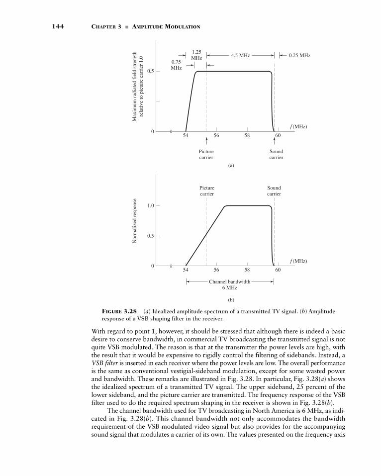
144 CHAPTER 3 � AMPLITUDE MODULATION
f (MHz)
(a)
Soundcarrier
Picturecarrier
Soundcarrier
Picturecarrier
0.75MHz
1.25MHz 4.5 MHz 0.25 MHz
54 56 58 600
0.5
Max
imum
rad
iate
d fi
eld
stre
ngth
rela
tive
to p
ictu
re c
arri
er 1
.0
≈
f (MHz)
(b)
54 56 58 600
1.0
0.5
Nor
mal
ized
res
pons
e
Channel bandwidth6 MHz
≈
FIGURE 3.28 (a) Idealized amplitude spectrum of a transmitted TV signal. (b) Amplituderesponse of a VSB shaping filter in the receiver.
With regard to point 1, however, it should be stressed that although there is indeed a basicdesire to conserve bandwidth, in commercial TV broadcasting the transmitted signal is notquite VSB modulated. The reason is that at the transmitter the power levels are high, withthe result that it would be expensive to rigidly control the filtering of sidebands. Instead, aVSB filter is inserted in each receiver where the power levels are low. The overall performanceis the same as conventional vestigial-sideband modulation, except for some wasted powerand bandwidth. These remarks are illustrated in Fig. 3.28. In particular, Fig. 3.28(a) showsthe idealized spectrum of a transmitted TV signal. The upper sideband, 25 percent of thelower sideband, and the picture carrier are transmitted. The frequency response of the VSBfilter used to do the required spectrum shaping in the receiver is shown in Fig. 3.28(b).
The channel bandwidth used for TV broadcasting in North America is 6 MHz, as indi-cated in Fig. 3.28(b). This channel bandwidth not only accommodates the bandwidthrequirement of the VSB modulated video signal but also provides for the accompanyingsound signal that modulates a carrier of its own. The values presented on the frequency axis
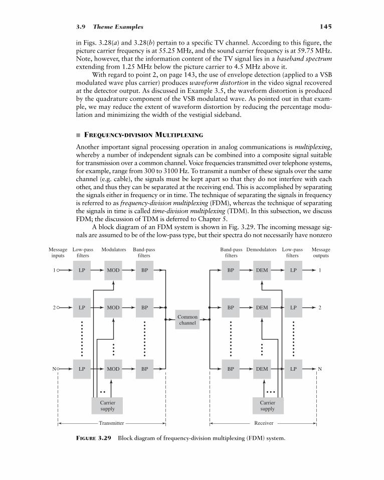
3.9 Theme Examples 145
in Figs. 3.28(a) and 3.28(b) pertain to a specific TV channel. According to this figure, thepicture carrier frequency is at 55.25 MHz, and the sound carrier frequency is at 59.75 MHz.Note, however, that the information content of the TV signal lies in a baseband spectrumextending from 1.25 MHz below the picture carrier to 4.5 MHz above it.
With regard to point 2, on page 143, the use of envelope detection (applied to a VSBmodulated wave plus carrier) produces waveform distortion in the video signal recoveredat the detector output. As discussed in Example 3.5, the waveform distortion is producedby the quadrature component of the VSB modulated wave. As pointed out in that exam-ple, we may reduce the extent of waveform distortion by reducing the percentage modu-lation and minimizing the width of the vestigial sideband.
� FREQUENCY-DIVISION MULTIPLEXING
Another important signal processing operation in analog communications is multiplexing,whereby a number of independent signals can be combined into a composite signal suitablefor transmission over a common channel. Voice frequencies transmitted over telephone systems,for example, range from 300 to 3100 Hz. To transmit a number of these signals over the samechannel (e.g. cable), the signals must be kept apart so that they do not interfere with eachother, and thus they can be separated at the receiving end. This is accomplished by separatingthe signals either in frequency or in time. The technique of separating the signals in frequencyis referred to as frequency-division multiplexing (FDM), whereas the technique of separatingthe signals in time is called time-division multiplexing (TDM). In this subsection, we discussFDM; the discussion of TDM is deferred to Chapter 5.
A block diagram of an FDM system is shown in Fig. 3.29. The incoming message sig-nals are assumed to be of the low-pass type, but their spectra do not necessarily have nonzero
LP
Messageinputs
Low-passfilters
Band-passfilters
Modulators
1 MOD BP
LP2 MOD BP
Commonchannel
LPN MOD
Carriersupply
Transmitter
LP
Low-passfilters
Messageoutputs
Band-passfilters
Demodulators
DEMBP
DEM
1
2
NDEM
Carriersupply
Receiver
BP BP LP
LPBP
FIGURE 3.29 Block diagram of frequency-division multiplexing (FDM) system.
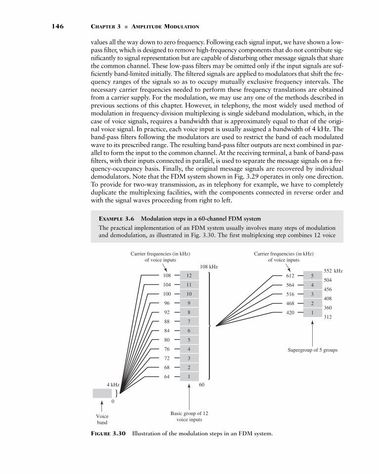
146 CHAPTER 3 � AMPLITUDE MODULATION
values all the way down to zero frequency. Following each signal input, we have shown a low-pass filter, which is designed to remove high-frequency components that do not contribute sig-nificantly to signal representation but are capable of disturbing other message signals that sharethe common channel. These low-pass filters may be omitted only if the input signals are suf-ficiently band-limited initially. The filtered signals are applied to modulators that shift the fre-quency ranges of the signals so as to occupy mutually exclusive frequency intervals. Thenecessary carrier frequencies needed to perform these frequency translations are obtainedfrom a carrier supply. For the modulation, we may use any one of the methods described inprevious sections of this chapter. However, in telephony, the most widely used method ofmodulation in frequency-division multiplexing is single sideband modulation, which, in thecase of voice signals, requires a bandwidth that is approximately equal to that of the origi-nal voice signal. In practice, each voice input is usually assigned a bandwidth of 4 kHz. Theband-pass filters following the modulators are used to restrict the band of each modulatedwave to its prescribed range. The resulting band-pass filter outputs are next combined in par-allel to form the input to the common channel. At the receiving terminal, a bank of band-passfilters, with their inputs connected in parallel, is used to separate the message signals on a fre-quency-occupancy basis. Finally, the original message signals are recovered by individualdemodulators. Note that the FDM system shown in Fig. 3.29 operates in only one direction.To provide for two-way transmission, as in telephony for example, we have to completelyduplicate the multiplexing facilities, with the components connected in reverse order andwith the signal waves proceeding from right to left.
EXAMPLE 3.6 Modulation steps in a 60-channel FDM system
The practical implementation of an FDM system usually involves many steps of modulationand demodulation, as illustrated in Fig. 3.30. The first multiplexing step combines 12 voice
12108
108 kHz
604 kHz
}
Voiceband
Basic group of 12voice inputs
0
5612
4564504
552 kHz
456
408
360
312
3516
2468
1420
11104
10100
996
892
788
684
580
476
372
268
164
Carrier frequencies (in kHz)of voice inputs
Supergroup of 5 groups
Carrier frequencies (in kHz)of voice inputs
FIGURE 3.30 Illustration of the modulation steps in an FDM system.
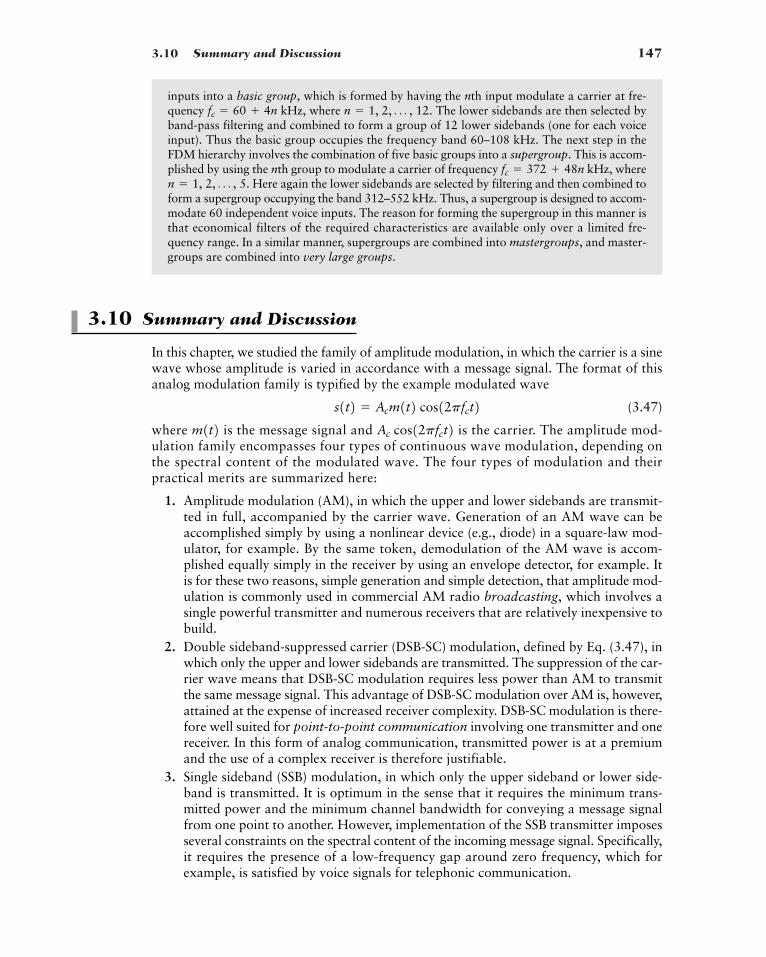
3.10 Summary and Discussion 147
inputs into a basic group, which is formed by having the nth input modulate a carrier at fre-quency kHz, where The lower sidebands are then selected byband-pass filtering and combined to form a group of 12 lower sidebands (one for each voiceinput). Thus the basic group occupies the frequency band 60–108 kHz. The next step in theFDM hierarchy involves the combination of five basic groups into a supergroup. This is accom-plished by using the nth group to modulate a carrier of frequency kHz, where
Here again the lower sidebands are selected by filtering and then combined toform a supergroup occupying the band 312–552 kHz. Thus, a supergroup is designed to accom-modate 60 independent voice inputs. The reason for forming the supergroup in this manner isthat economical filters of the required characteristics are available only over a limited fre-quency range. In a similar manner, supergroups are combined into mastergroups, and master-groups are combined into very large groups.
3.10 Summary and Discussion
In this chapter, we studied the family of amplitude modulation, in which the carrier is a sinewave whose amplitude is varied in accordance with a message signal. The format of thisanalog modulation family is typified by the example modulated wave
(3.47)
where is the message signal and is the carrier. The amplitude mod-ulation family encompasses four types of continuous wave modulation, depending onthe spectral content of the modulated wave. The four types of modulation and theirpractical merits are summarized here:
1. Amplitude modulation (AM), in which the upper and lower sidebands are transmit-ted in full, accompanied by the carrier wave. Generation of an AM wave can beaccomplished simply by using a nonlinear device (e.g., diode) in a square-law mod-ulator, for example. By the same token, demodulation of the AM wave is accom-plished equally simply in the receiver by using an envelope detector, for example. Itis for these two reasons, simple generation and simple detection, that amplitude mod-ulation is commonly used in commercial AM radio broadcasting, which involves asingle powerful transmitter and numerous receivers that are relatively inexpensive tobuild.
2. Double sideband-suppressed carrier (DSB-SC) modulation, defined by Eq. (3.47), inwhich only the upper and lower sidebands are transmitted. The suppression of the car-rier wave means that DSB-SC modulation requires less power than AM to transmitthe same message signal. This advantage of DSB-SC modulation over AM is, however,attained at the expense of increased receiver complexity. DSB-SC modulation is there-fore well suited for point-to-point communication involving one transmitter and onereceiver. In this form of analog communication, transmitted power is at a premiumand the use of a complex receiver is therefore justifiable.
3. Single sideband (SSB) modulation, in which only the upper sideband or lower side-band is transmitted. It is optimum in the sense that it requires the minimum trans-mitted power and the minimum channel bandwidth for conveying a message signalfrom one point to another. However, implementation of the SSB transmitter imposesseveral constraints on the spectral content of the incoming message signal. Specifically,it requires the presence of a low-frequency gap around zero frequency, which forexample, is satisfied by voice signals for telephonic communication.
Ac cos12pfct2m1t2s1t2 � Acm1t2 cos12pfct2
n � 1, 2, Á , 5.fc � 372 48n
n � 1, 2, Á , 12.fc � 60 4n
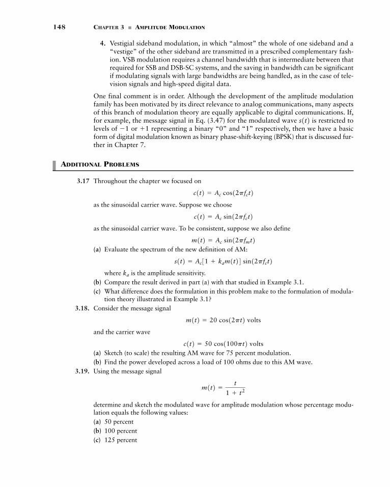
148 CHAPTER 3 � AMPLITUDE MODULATION
4. Vestigial sideband modulation, in which “almost” the whole of one sideband and a“vestige” of the other sideband are transmitted in a prescribed complementary fash-ion. VSB modulation requires a channel bandwidth that is intermediate between thatrequired for SSB and DSB-SC systems, and the saving in bandwidth can be significantif modulating signals with large bandwidths are being handled, as in the case of tele-vision signals and high-speed digital data.
One final comment is in order. Although the development of the amplitude modulationfamily has been motivated by its direct relevance to analog communications, many aspectsof this branch of modulation theory are equally applicable to digital communications. If,for example, the message signal in Eq. (3.47) for the modulated wave is restricted tolevels of or representing a binary “0” and “1” respectively, then we have a basicform of digital modulation known as binary phase-shift-keying (BPSK) that is discussed fur-ther in Chapter 7.
ADDITIONAL PROBLEMS
3.17 Throughout the chapter we focused on
as the sinusoidal carrier wave. Suppose we choose
as the sinusoidal carrier wave. To be consistent, suppose we also define
(a) Evaluate the spectrum of the new definition of AM:
where is the amplitude sensitivity.(b) Compare the result derived in part (a) with that studied in Example 3.1.(c) What difference does the formulation in this problem make to the formulation of modula-
tion theory illustrated in Example 3.1?3.18. Consider the message signal
and the carrier wave
(a) Sketch (to scale) the resulting AM wave for 75 percent modulation.(b) Find the power developed across a load of 100 ohms due to this AM wave.
3.19. Using the message signal
determine and sketch the modulated wave for amplitude modulation whose percentage modu-lation equals the following values:(a) 50 percent(b) 100 percent(c) 125 percent
m1t2 �t
1 t2
c1t2 � 50 cos1100pt2 volts
m1t2 � 20 cos12pt2 volts
ka
s1t2 � Ac31 kam1t24 sin12pfct2m1t2 � Ac sin12pfmt2c1t2 � Ac sin12pfct2c1t2 � Ac cos12pfct2
1�1s1t2
Additional Problems 149
3.20 Suppose a nonlinear device is available for which the output current and input voltage arerelated by
where and are constants. Explain how such a device could be used to provide amplitudemodulation. Could such a device also be used for demodulation? Justify your answer.
3.21 Consider the DSB-SC modulated wave obtained by using the sinusoidal modulating wave
and the carrier wave
The phase angle denoting the phase difference between and at time is vari-able. Sketch this modulated wave for the following values of (a)(b)(c)(d)Comment on your results.
3.22 Given the nonlinear device described in Problem 3.20, explain how it could be used to providea product modulator.
3.23 Consider a message signal with the spectrum shown in Fig. 3.31. The message bandwidthThis signal is applied to a product modulator, together with a carrier wave
producing the DSB-SC modulated wave This modulated wave is nextapplied to a coherent detector. Assuming perfect synchronism between the carrier waves in themodulator and detector, determine the spectrum of the detector output when: (a) the carrier fre-quency and (b) the carrier frequency What is the lowest carrierfrequency for which each component of the modulated wave is uniquely determinedby m1t2? s1t2fc � 0.75 kHz.fc � 1.25 kHz
s1t2.Ac cos12pfct2,W � 1 kHz.m1t2
f � 135°f � 90°f � 45°f � 0
f:t � 0,m1t2c1t2f,
c1t2 � Ac cos12pfct f2m1t2 � Am cos12pfmt2
a3a1
io � a1ni a3ni3
niio
f–W W
M( f )
0 FIGURE 3.31 Problem 3.23
3.24 Consider a composite wave obtained by adding a noncoherent carrier to aDSB-SC wave This composite wave is applied to an ideal envelope detector.Find the resulting detector output for(a)(b) and
3.25 A DSB-SC wave is demodulated by applying it to a coherent detector.(a) Evaluate the effect of a frequency error in the local carrier frequency of the detector, mea-
sured with respect to the carrier frequency of the incoming DSB-SC wave.(b) For the case of a sinusoidal modulating wave, show that because of this frequency error, the
demodulated wave exhibits beats at the error frequency. Illustrate your answer with a sketchof this demodulated wave. (A beat refers to a signal whose frequency is the differencebetween the frequencies of two input signals.)
¢f
ƒm1t2 ƒ V Ac>2f 0f � 0
cos12pfct2m1t2. Ac cos12pfct f2
150 CHAPTER 3 � AMPLITUDE MODULATION
3.26 Consider a pulse of amplitude A and duration T. This pulse is applied to a SSB modulator, pro-ducing the modulated wave Determine the envelope of and show that this envelopeexhibits peaks at the beginning and end of the pulse.
3.27 (a) Consider a message signal containing frequency components at 100, 200, and 400Hz. This signal is applied to a SSB modulator together with a carrier at 100 kHz, with onlythe upper sideband retained. In the coherent detector used to recover the local oscil-lator supplies a sinusoidal wave of frequency 100.02 kHz. Determine the frequency com-ponents of the detector output.
(b) Repeat your analysis, assuming that only the lower sideband is transmitted.3.28 Throughout this chapter, we have expressed the sinusoidal carrier wave in the form
where is the carrier amplitude and is the carrier frequency. In Chapter 7 dealing with dig-ital band-pass modulation techniques, we find it more convenient to express the carrier in theform
where is the duration allotted to the transmission of symbol 1 or symbol 0. Determine thevalue of carrier amplitude for the energy in per symbol to equal unity.
ADVANCED PROBLEMS
3.29 For a p-n junction diode, the current i through the diode and the voltage across it are related by
where is the reverse saturation current and is the thermal voltage defined by
where k is Boltzmann’s constant in joules per degree Kelvin, T is the absolute temperature indegrees Kelvin, and e is the charge of an electron. At room temperature, (a) Expand i as a power series in retaining terms up to (b) Let
where and Determine the spectrum of the resulting diode cur-rent i.
(c) Specify the bandpass filter required to extract from the diode current an AM wave withcarrier frequency
(d) What is the percentage modulation of this AM wave?3.30 Consider the quadrature-carrier multiplex system of Fig. 3.17. The multiplexed signal pro-
duced at the transmitter output in part (a) of this figure is applied to a communication channelof transfer function The output of this channel is, in turn, applied to the receiver inputin part (b) of Fig. 3.17. Prove that the condition
H1fc f2 � H*1fc � f2, for 0 � f � W
H1f2.s1t2
fc .
fc � 100 kHz.fm � 1 kHz
v � 0.01 cos12pfmt2 0.01 cos12pfct2 volts
n3.n,VT � 0.026 volt.
VT �kTe
VTI0
i � I0Bexp¢�n
VT≤ � 1R n
c1t2Ac
Tb
c1t2 � A 2Tb
cos12pfct2
fcAc
c1t2 � Ac cos12pfct2
m1t2,m1t2
s1t2,s1t2.
Advanced Problems 151
is necessary for recovery of the message signals and at the receiver outputs; isthe carrier frequency, W is the message bandwidth. The asterisk in denotes com-plex conjugation. Hint: Evaluate the spectra of the two receiver outputs.
3.31 (a) Let denote the SSB wave obtained by transmitting only the upper sideband, and its Hilbert transform. Show that
and
where is the message signal, is its Hilbert transform, the carrier frequency,and is the carrier amplitude.
(b) Show that the corresponding equations in terms of the SSB wave obtained by trans-mitting only the lower sideband are
and
(c) Using the results of (a) and (b), set up the block diagrams of a receiver for demodulating anSSB wave.
Note: The Hilbert transform is defined in Problem 2.52; see also footnote 4 of this chapter.3.32 In this problem, we continue the discussion on VSB modulation for the case when a vestige of
the lower sideband is transmitted; Fig. 3.24 depicts the frequency response of the sidebandshaping filter used to generate such a modulated wave. In particular, we wish to examine thecomplex representation of this filter, denoted by
Let and denote the in-phase and quadrature components of respec-tively. Show that over the interval we have(a) represents an all-pass filter; that is, the frequency response of the filter is constant as
shown by
where W is the message bandwidth.(b) represents a low-pass filter with an odd-symmetric frequency response, described by
the following three relations
1.
2.
3.
where is the width of the vestigial sideband.fv
HQ1f2 � 1 for fv � f � W
HQ102 � 0
HQ1�f2 � �HQ1f2, �W � f � W
HQ1f2H1f2 � 1, for �W � f � W
HI1f2�W � f � W,
H'1f2,HQ1f2HI1f2 H
'1f2.H1f2
mn 1t2 �2Ac3sl1t2 cos12pfct2 � snl1t2 sin12pfct24
m1t2 �2Ac3sl1t2 cos12pfct2 snl1t2 sin12pfct24
sl1t2Ac
fcmn 1t2m1t2mn 1t2 �
2Ac3snu1t2 cos12pfct2 � su1t2 sin12pfct24
m1t2 �2Ac3su1t2 cos12pfct2 snu1t2 sin12pfct24
snu1t2su1t2
H*1fc � f2 fcm21t2m11t2
152
CHAPTER 4
ANGLE MODULATION
In the previous chapter, we investigated the effect of slowly varying the amplitude of asinusoidal carrier wave in accordance with an information-bearing signal, keeping the car-rier frequency fixed. There is another way of modulating a sinusoidal carrier wave—namely, angle modulation, in which the angle of the carrier wave is varied according to theinformation-bearing signal. In this second family of modulation techniques, the amplitudeof the carrier wave is maintained constant.
An important feature of angle modulation is that it can provide better discriminationagainst noise and interference than amplitude modulation. As will be shown in Chapter 9,however, this improvement in performance is achieved at the expense of increased trans-mission bandwidth; that is, angle modulation provides us with a practical means ofexchanging channel bandwidth for improved noise performance. Such a tradeoff is notpossible with amplitude modulation. Moreover, the improvement in noise performance inangle modulation is achieved at the cost of increased system complexity in both the trans-mitter and receiver.
The material presented in this chapter on angle modulation will teach us threelessons:
� Lesson 1: Angle modulation is a nonlinear process, which testifies to its sophisticatednature. In the context of analog communications, this distinctive property of angle modu-lation has two implications:
� In analytic terms, the spectral analysis of angle modulation is complicated.
� In practical terms, the implementation of angle modulation is demanding.
Both of these statements are made with amplitude modulation as the frame of reference.
� Lesson 2: Whereas the transmission bandwidth of an amplitude-modulated wave (or anyof its variants) is of limited extent, the transmission bandwidth of an angle-modulatedwave may assume an infinite extent, at least in theory.
� Lesson 3: Given that the amplitude of the carrier wave is maintained constant, we wouldintuitively expect that additive noise would affect the performance of angle modulation toa lesser extent than amplitude modulation.
4.1 Basic Definitions 153
4.1 Basic Definitions
Let denote the angle of a modulated sinusoidal carrier at time t; it is assumed to be afunction of the information-bearing signal or message signal. We express the resultingangle-modulated wave as
(4.1)
where is the carrier amplitude. A complete oscillation occurs whenever the angle changes by radians. If increases monotonically with time, then the average fre-quency in hertz, over a small interval from t to is given by
Allowing the time interval to approach zero leads to the following definition for theinstantaneous frequency of the angle-modulated signal
(4.2)
where, in the last line, we have invoked the definition for the derivative of the angle with respect to time t.
Thus according to Eq. (4.1), we may interpret the angle-modulated signal as arotating phasor of length and angle The angular velocity of such a phasor is
measured in radians per second. In the simple case of an unmodulated carrier, theangle is
and the corresponding phasor rotates with a constant angular velocity equal to radi-ans per second. The constant defines the angle of the unmodulated carrier at time
There are an infinite number of ways in which the angle may be varied in somemanner with the message signal. However, we shall consider only two commonly usedmethods, phase modulation and frequency modulation, as defined below:
1. Phase modulation (PM) is that form of angle modulation in which the instantaneousangle is varied linearly with the message signal as shown by
(4.3)
The term represents the angle of the unmodulated carrier with the constant set equal to zero for convenience of presentation; the constant represents the phasesensitivity factor of the modulator, expressed in radians per volt on the assumptionthat is a voltage waveform. The phase-modulated wave is correspondinglydescribed in the time domain by
(4.4)s1t2 � Ac cos32pfc t kpm1t24s1t2m1t2kp
fc2pfct
ui1t2 � 2pfc t kpm1t2m1t2,ui1t2
ui1t2 t � 0.fc
2pfc
ui1t2 � 2pfct fc , for m1t2 � 0
ui1t2dui1t2>dt,ui1t2.Ac
s1t2ui1t2
�1
2p
dui1t2dt
� lim¢tS0
B ut1t ¢t2 � ui1t22p¢t
Rfi1t2 � lim¢tS0
f¢t1t2s1t2:¢t
f¢t1t2 �ut1t ¢t2 � ui1t2
2p¢t
t ¢t,ui1t22p
ui1t2Ac
s1t2 � Ac cos3ui1t24
ui1t2
154 CHAPTER 4 � ANGLE MODULATION
2. Frequency modulation (FM) is that form of angle modulation in which the instanta-neous frequency is varied linearly with the message signal as shown by
(4.5)
The constant term represents the frequency of the unmodulated carrier; the constantrepresents the frequency-sensitivity factor of the modulator, expressed in hertz per
volt on the assumption that is a voltage waveform. Integrating Eq. (4.5) withrespect to time and multiplying the result by we get
(4.6)
where the second term accounts for the increase or decrease in the instantaneousphase due to the message signal The frequency-modulated wave is therefore
(4.7)
Table 4.1 summarizes the basic definitions embodied in the generation of angle-modulated waves.These definitions apply to all kinds of message signals, be they of the analog or digital kind.
s1t2 � Ac cos c2pfct 2pkfLt
0m1t2 dt d
m1t2.ui1t2
� 2pfct 2pkfLt
0m1t2 dt
ui1t2 � 2pLt
0fi1t2 dt
2p,m1t2kf
fc
fi1t2 � fc kf m1t2m1t2,fi1t2
TABLE 4.1 Summary of Basic Definitions in Angle Modulation
Phase modulation Frequency modulation Comments
Instantaneousphase
Instantaneous
frequency
Modulatedwave s1t2 Ac cos c2pfct 2pkfL
t
0m1t2 dt dAc cos32pfct kpm1t24
fi1t2fc kf m1t2fc
kp
2pddt
m1t2
ui1t22pfct 2pkfL
t
0m1t2 dt2pfct kpm1t2 carrier amplitude
carrier frequencymessage signal
phase-sensitivityfactorfrequency-sensitivityfactor
kf:
kp:m1t2:fc:Ac:
4.2 Properties of Angle-Modulated Waves
Angle-modulated waves are characterized by some important properties, which follow fromthe basic definitions summarized in Table 4.1. Indeed, it is these properties that put angle-mod-ulated waves in a family of their own, and distinguish them from the family of amplitude-modulated waves, as illustrated by the waveforms shown in Fig. 4.1 for the example ofsinusoidal modulation. Figures 4.1(a) and 4.1(b) are the sinusoidal carrier and modulatingwaves, respectively. Figures 4.1(c), 4.1(d), and 4.1(e) display the corresponding amplitude-mod-ulated (AM), phase-modulated (PM), and frequency-modulated (FM) waves, respectively.
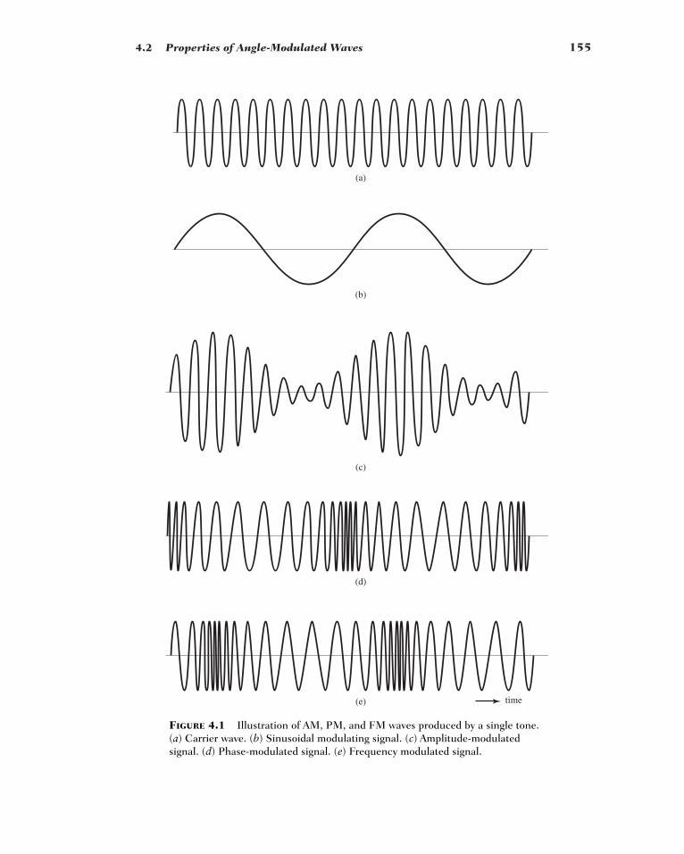
4.2 Properties of Angle-Modulated Waves 155
(a)
(b)
(c)
(d)
(e) time
FIGURE 4.1 Illustration of AM, PM, and FM waves produced by a single tone.(a) Carrier wave. (b) Sinusoidal modulating signal. (c) Amplitude-modulatedsignal. (d) Phase-modulated signal. (e) Frequency modulated signal.
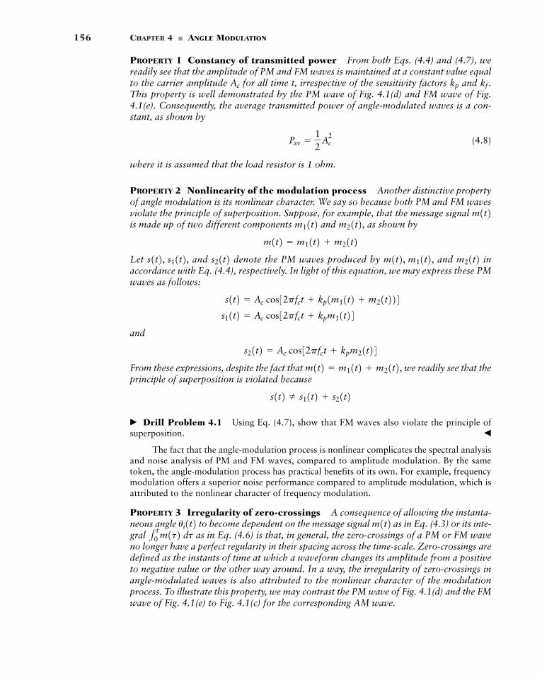
156 CHAPTER 4 � ANGLE MODULATION
PROPERTY 1 Constancy of transmitted power From both Eqs. (4.4) and (4.7), wereadily see that the amplitude of PM and FM waves is maintained at a constant value equalto the carrier amplitude for all time t, irrespective of the sensitivity factors and This property is well demonstrated by the PM wave of Fig. 4.1(d) and FM wave of Fig.4.1(e). Consequently, the average transmitted power of angle-modulated waves is a con-stant, as shown by
(4.8)
where it is assumed that the load resistor is 1 ohm.
PROPERTY 2 Nonlinearity of the modulation process Another distinctive propertyof angle modulation is its nonlinear character. We say so because both PM and FM wavesviolate the principle of superposition. Suppose, for example, that the message signal is made up of two different components and as shown by
Let and denote the PM waves produced by and inaccordance with Eq. (4.4), respectively. In light of this equation, we may express these PMwaves as follows:
and
From these expressions, despite the fact that we readily see that theprinciple of superposition is violated because
� Drill Problem 4.1 Using Eq. (4.7), show that FM waves also violate the principle ofsuperposition. �
The fact that the angle-modulation process is nonlinear complicates the spectral analysisand noise analysis of PM and FM waves, compared to amplitude modulation. By the sametoken, the angle-modulation process has practical benefits of its own. For example, frequencymodulation offers a superior noise performance compared to amplitude modulation, which isattributed to the nonlinear character of frequency modulation.
PROPERTY 3 Irregularity of zero-crossings A consequence of allowing the instanta-neous angle to become dependent on the message signal as in Eq. (4.3) or its inte-gral as in Eq. (4.6) is that, in general, the zero-crossings of a PM or FM waveno longer have a perfect regularity in their spacing across the time-scale. Zero-crossings aredefined as the instants of time at which a waveform changes its amplitude from a positiveto negative value or the other way around. In a way, the irregularity of zero-crossings inangle-modulated waves is also attributed to the nonlinear character of the modulationprocess. To illustrate this property, we may contrast the PM wave of Fig. 4.1(d) and the FMwave of Fig. 4.1(e) to Fig. 4.1(c) for the corresponding AM wave.
1 t0 m1t2 dt
m1t2ui1t2
s1t2 s11t2 s21t2m1t2 � m11t2 m21t2,
s21t2 � Ac cos32pfct kpm21t24s11t2 � Ac cos32pfct kpm11t24s1t2 � Ac cos32pfct kp1m11t2 m21t224
m21t2m1t2, m11t2,s21t2s1t2, s11t2,m1t2 � m11t2 m21t2
m21t2,m11t2 m1t2
Pav �12
Ac2
kf .kpAc
4.2 Properties of Angle-Modulated Waves 157
However, we may cite two special cases where regularity is maintained in anglemodulation:
1. The message signal increases or decreases linearly with time t, in which case theinstantaneous frequency of the PM wave changes from the unmodulated carrierfrequency to a new constant value dependent on the slope of
2. The message signal is maintained at some constant value, positive or negative,in which case the instantaneous frequency of the FM wave changes from theunmodulated carrier frequency to a new constant value dependent on the constantvalue of
In any event, it is important to note that in angle modulation, the information content ofthe message signal resides in the zero-crossings of the modulated wave. This statementholds provided the carrier frequency is large compared to the highest frequency compo-nent of the message signal
PROPERTY 4 Visualization difficulty of message waveform In AM, we see the mes-sage waveform as the envelope of the modulated wave, provided, of course, the percent-age modulation is less than 100 percent, as illustrated in Fig. 4.1(c) for sinusoidalmodulation. This is not so in angle modulation, as illustrated by the corresponding wave-forms of Figs. 4.1(d) and 4.1(e) for PM and FM, respectively. In general, the difficulty invisualizing the message waveform in angle-modulated waves is also attributed to the non-linear character of angle-modulated waves.
PROPERTY 5 Tradeoff of increased transmission bandwidth for improved noiseperformance An important advantage of angle modulation over amplitude modulationis the realization of improved noise performance. This advantage is attributed to the factthat the transmission of a message signal by modulating the angle of a sinusoidal carrierwave is less sensitive to the presence of additive noise than transmission by modulatingthe amplitude of the carrier. The improvement in noise performance is, however, attainedat the expense of a corresponding increase in the transmission bandwidth requirement ofangle modulation. In other words, the use of angle modulation offers the possibility ofexchanging an increase in transmission bandwidth for an improvement in noise perfor-mance. Such a tradeoff is not possible with amplitude modulation since the transmissionbandwidth of an amplitude-modulated wave is fixed somewhere between the messagebandwidth W and 2W, depending on the type of modulation employed. The effect of noiseon angle modulation is discussed in Chapter 9.
EXAMPLE 4.1 Zero-crossings
Consider a modulating wave that increases linearly with time t, starting at asshown by
where a is the slope parameter; see Fig. 4.2(a). In what follows, we study the zero-crossings ofthe PM and FM waves produced by for the following set of parameters:
a � 1 volt>sfc �
14
Hz
m1t2
m1t2 � bat, t � 00, t � 0
t � 0,m1t2
m1t2. fcm1t2
m1t2. fcfi1t2m1t2 m1t2.fc
fi1t2m1t2
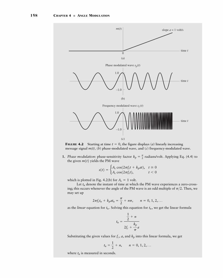
158 CHAPTER 4 � ANGLE MODULATION
Phase modulated wave sp(t)
time t
1.0
–1.0
Frequency modulated wave sf (t)
time t
1.0
–1.0
(a)
(b)
(c)
slope a = 1 volt/s
time t0
m(t)
1. Phase modulation: phase-sensitivity factor radians/volt. Applying Eq. (4.4) tothe given yields the PM wave
which is plotted in Fig. 4.2(b) for Let denote the instant of time at which the PM wave experiences a zero-cross-
ing; this occurs whenever the angle of the PM wave is an odd multiple of Then, wemay set up
as the linear equation for Solving this equation for we get the linear formula
Substituting the given values for a, and into this linear formula, we get
where is measured in seconds.tn
tn �12
n, n � 0, 1, 2, Á
kpfc ,
tn �
12
n
2fc kp
pa
tn ,tn .
2pfctn kpatn �p
2 np, n � 0, 1, 2, Á
p>2.tn
Ac � 1 volt.
s1t2 � bAc cos12pfct kpat2, t � 0Ac cos12pfct2, t � 0
m1t2 kp � p
2
FIGURE 4.2 Starting at time the figure displays (a) linearly increasingmessage signal m(t), (b) phase-modulated wave, and (c) frequency-modulated wave.
t � 0,
4.3 Relationship Between PM and FM Waves 159
2. Frequency modulation: frequency-sensitivity factor, Applying Eq. (4.7)yields the FM wave
which is plotted in Fig. 4.2(c).Invoking the definition of a zero-crossing, we may set up
as the quadratic equation for The positive root of this equation—namely,
defines the formula for Substituting the given values of a, and into this quadraticformula, we get
where is again measured in seconds.
Comparing the zero-crossing results derived for PM and FM waves, we may make thefollowing observations once the linear modulating wave begins to act on the sinusoidal carrierwave:
1. For PM, regularity of the zero-crossings is maintained; the instantaneous frequencychanges from the unmodulated value of to the new constant value of
2. For FM, the zero-crossings assume an irregular form; as expected, the instantaneous fre-quency increases linearly with time t.
The angle-modulated waveforms of Fig. 4.2 should be contrasted with the correspondingones of Fig. 4.1. Whereas in the case of sinusoidal modulation depicted in Fig. 4.1 it is dif-ficult to discern the difference between PM and FM, this is not so in the case of Fig. 4.2.In other words, depending on the modulating wave, it is possible for PM and FM to exhibitentirely different waveforms.
4.3 Relationship Between PM and FM Waves
Examining the definitions of Eqs. (4.4) and (4.7), we see that an FM wave may be viewedas a PM wave produced by the modulating wave in place of This meansthat an FM wave can be generated by first integrating the message signal with respectto time t and then using the resulting signal as the input to a phase modulator, as shownin Fig. 4.3(a).
Conversely, a PM wave can be viewed as an FM wave produced by the modulatingwave Hence, a PM wave can be generated by first differentiating withrespect to time t and then using the resulting signal as the input to a frequency modulator,as shown in Fig. 4.3(b).
m1t2dm1t2>dt.
m1t2m1t2.1 t0 m1t2 dt
fc kp1a>2p2 �12
Hz.
fc � 1>4 Hz
tn
tn �14A�1 29 16n B , n � 0, 1, 2, Á
kffc ,tn .
tn �1
akf¢�fc Bf c
2 akf a1
2 nb ≤ , n � 0, 1, 2, Á
tn .
2pfctn pkf atn2
�p
2 np, n � 0, 1, 2, Á
s1t2 � bAc cos12pfct pkfat22, t � 0Ac cos12pfct2, t � 0
kf � 1 Hz>volt.
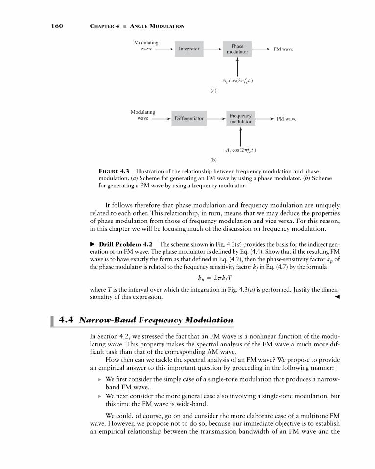
160 CHAPTER 4 � ANGLE MODULATION
(a)
Ac cos(2�fct )
Modulatingwave Integrator Phase
modulator FM wave
(b)
Ac cos(2�fct )
Modulatingwave Differentiator Frequency
modulator PM wave
FIGURE 4.3 Illustration of the relationship between frequency modulation and phasemodulation. (a) Scheme for generating an FM wave by using a phase modulator. (b) Schemefor generating a PM wave by using a frequency modulator.
It follows therefore that phase modulation and frequency modulation are uniquelyrelated to each other. This relationship, in turn, means that we may deduce the propertiesof phase modulation from those of frequency modulation and vice versa. For this reason,in this chapter we will be focusing much of the discussion on frequency modulation.
� Drill Problem 4.2 The scheme shown in Fig. 4.3(a) provides the basis for the indirect gen-eration of an FM wave. The phase modulator is defined by Eq. (4.4). Show that if the resulting FMwave is to have exactly the form as that defined in Eq. (4.7), then the phase-sensitivity factor ofthe phase modulator is related to the frequency sensitivity factor in Eq. (4.7) by the formula
where T is the interval over which the integration in Fig. 4.3(a) is performed. Justify the dimen-sionality of this expression. �
4.4 Narrow-Band Frequency Modulation
In Section 4.2, we stressed the fact that an FM wave is a nonlinear function of the modu-lating wave. This property makes the spectral analysis of the FM wave a much more dif-ficult task than that of the corresponding AM wave.
How then can we tackle the spectral analysis of an FM wave? We propose to providean empirical answer to this important question by proceeding in the following manner:
� We first consider the simple case of a single-tone modulation that produces a narrow-band FM wave.
� We next consider the more general case also involving a single-tone modulation, butthis time the FM wave is wide-band.
We could, of course, go on and consider the more elaborate case of a multitone FMwave. However, we propose not to do so, because our immediate objective is to establishan empirical relationship between the transmission bandwidth of an FM wave and the
kp � 2pkfT
kf
kp
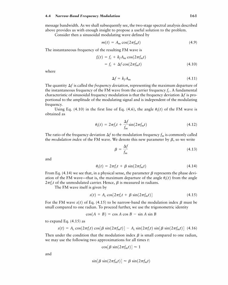
4.4 Narrow-Band Frequency Modulation 161
message bandwidth. As we shall subsequently see, the two-stage spectral analysis describedabove provides us with enough insight to propose a useful solution to the problem.
Consider then a sinusoidal modulating wave defined by
(4.9)
The instantaneous frequency of the resulting FM wave is
(4.10)
where
(4.11)
The quantity is called the frequency deviation, representing the maximum departure ofthe instantaneous frequency of the FM wave from the carrier frequency A fundamentalcharacteristic of sinusoidal frequency modulation is that the frequency deviation is pro-portional to the amplitude of the modulating signal and is independent of the modulatingfrequency.
Using Eq. (4.10) in the first line of Eq. (4.6), the angle of the FM wave isobtained as
(4.12)
The ratio of the frequency deviation to the modulation frequency is commonly calledthe modulation index of the FM wave. We denote this new parameter by so we write
(4.13)
and
(4.14)
From Eq. (4.14) we see that, in a physical sense, the parameter represents the phase devi-ation of the FM wave—that is, the maximum departure of the angle from the angle
of the unmodulated carrier. Hence, is measured in radians.The FM wave itself is given by
(4.15)
For the FM wave of Eq. (4.15) to be narrow-band the modulation index must besmall compared to one radian. To proceed further, we use the trigonometric identity
to expand Eq. (4.15) as
(4.16)
Then under the condition that the modulation index is small compared to one radian,we may use the following two approximations for all times t:
and
sin3b sin12pfmt24 � b sin12pfmt2cos3b sin12pfmt24 � 1
b
s1t2 � Ac cos12pfct2 cos3b sin12pfmt24 � Ac sin12pfct2 sin3b sin12pfmt24cos1A B2 � cos A cos B � sin A sin B
bs1t2s1t2 � Ac cos32pfct b sin12pfmt24
b2pfctui1t2b
ui1t2 � 2pfct b sin12pfmt2
b �¢f
fm
b,fm¢f
ui1t2 � 2pfct ¢f
fmsin12pfmt2
ui1t2¢f
fc .¢f
¢f � kf Am
� fc ¢f cos12pfmt2fi1t2 � fc kf Am cos12pfmt2
m1t2 � Am cos12pfmt2
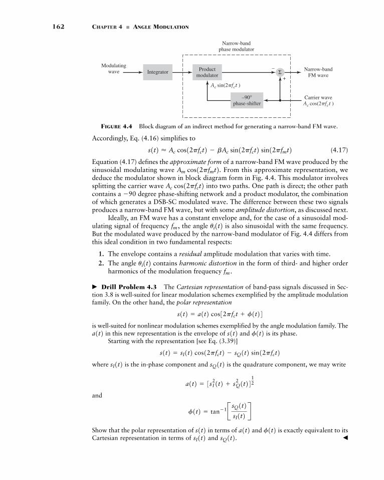
162 CHAPTER 4 � ANGLE MODULATION
Ac sin(2�fct )
Modulatingwave Integrator Product
modulatorNarrow-band
FM wave
Carrier waveAc cos(2�fct )
–90°phase-shifter
–
+Σ
Narrow-bandphase modulator
FIGURE 4.4 Block diagram of an indirect method for generating a narrow-band FM wave.
Accordingly, Eq. (4.16) simplifies to
(4.17)
Equation (4.17) defines the approximate form of a narrow-band FM wave produced by thesinusoidal modulating wave From this approximate representation, wededuce the modulator shown in block diagram form in Fig. 4.4. This modulator involvessplitting the carrier wave into two paths. One path is direct; the other pathcontains a degree phase-shifting network and a product modulator, the combinationof which generates a DSB-SC modulated wave. The difference between these two signalsproduces a narrow-band FM wave, but with some amplitude distortion, as discussed next.
Ideally, an FM wave has a constant envelope and, for the case of a sinusoidal mod-ulating signal of frequency the angle is also sinusoidal with the same frequency.But the modulated wave produced by the narrow-band modulator of Fig. 4.4 differs fromthis ideal condition in two fundamental respects:
1. The envelope contains a residual amplitude modulation that varies with time.2. The angle contains harmonic distortion in the form of third- and higher order
harmonics of the modulation frequency
� Drill Problem 4.3 The Cartesian representation of band-pass signals discussed in Sec-tion 3.8 is well-suited for linear modulation schemes exemplified by the amplitude modulationfamily. On the other hand, the polar representation
is well-suited for nonlinear modulation schemes exemplified by the angle modulation family. Thein this new representation is the envelope of and is its phase.Starting with the representation [see Eq. (3.39)]
where is the in-phase component and is the quadrature component, we may write
and
Show that the polar representation of in terms of and is exactly equivalent to itsCartesian representation in terms of and �sQ1t2.sI1t2 f1t2a1t2s1t2
f1t2 � tan�1B sQ1t2sI1t2 R
a1t2 � 3sI21t2 sQ
2 1t2412sQ1t2sI1t2
s1t2 � sI1t2 cos12pfct2 � sQ1t2 sin12pfct2f1t2s1t2a1t2
s1t2 � a1t2 cos32pfct f1t24
fm .ui1t2
ui1t2fm ,
�90Ac cos12pfct2
Am cos12pfmt2.s1t2 � Ac cos12pfct2 � bAc sin12pfct2 sin12pfmt2
4.4 Narrow-Band Frequency Modulation 163
� Drill Problem 4.4 Consider the narrow-band FM wave approximately defined by Eq.(4.17). Building on Problem 4.3, do the following:
(a) Determine the envelope of this modulated wave. What is the ratio of the maximum to theminimum value of this envelope?
(b) Determine the average power of the narrow-band FM wave, expressed as a percentage ofthe average power of the unmodulated carrier wave.
(c) By expanding the angular argument of the narrow-band FM wavein the form of a power series, and restricting the modulation index to a maximum
value of 0.3 radian, show that
What is the value of the harmonic distortion for radian?
Hint: For small x, the following power series approximation
holds. In this approximation, terms involving and higher order ones are ignored, which isjustified when x is small compared to unity. �
The important point to note from Problem 4.4 is that by restricting the modulationindex to radian, the effects of residual amplitude modulation and harmonic dis-tortion are limited to negligible levels. We are therefore emboldened to proceed furtherwith the use of Eq. (4.17), provided radian. In particular, we may expand themodulated wave further into three frequency components:
(4.18)
This expression is somewhat similar to the corresponding one defining an AM wave, whichis reproduced from Example 3.1 of Chapter 3 as follows:
(4.19)
where is the modulation factor of the AM signal. Comparing Eqs. (4.18) and (4.19) andputting aside the respective constants and we see that in the case of sinusoidal mod-ulation, the basic difference between an AM wave and a narrow-band FM wave is that thealgebraic sign of the lower side-frequency in the narrow-band FM is reversed. Neverthe-less, a narrow-band FM wave requires essentially the same transmission bandwidth (i.e.,
for sinusoidal modulation) as the AM wave.
� PHASOR INTERPRETATION
We may represent the narrow-band FM wave with a phasor diagram as shown in Fig. 4.5(a),where we have used the carrier phasor as reference. We see that the resultant of the two side-frequency phasors is always at right angles to the carrier phasor. The effect of this geometry isto produce a resultant phasor representing the narrow-band FM wave that is approximatelyof the same amplitude as the carrier phasor, but out of phase with respect to it.
2fm
m,b
m
sAM1t2 � Ac cos12pfct2 12mAc5cos32p1fc fm2t4 cos32p1fc � fm2t46
s1t2 � Ac cos12pfct2 12bAc5cos32p1fc fm2t4 � cos32p1fc � fm2t46
b � 0.3
b � 0.3
x5
tan�11x2 � x �13
x3
b � 0.3
u1t2 � 2pfct b sin12pfmt2 �b3
3 sin312pfmt2
bs1t2 u1t2 � 2pfct f1t2
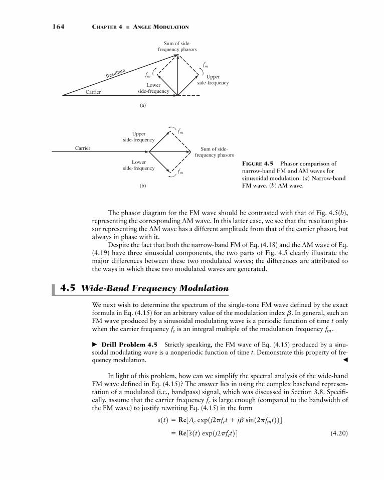
164 CHAPTER 4 � ANGLE MODULATION
(a)
(b)
Carrier
Lowerside-frequency
Upperside-frequency
Sum of side-frequency phasors
fm
fm
Resultant
CarrierLower
side-frequency
Upperside-frequency
fm
fm
Sum of side-frequency phasors
FIGURE 4.5 Phasor comparison ofnarrow-band FM and AM waves forsinusoidal modulation. (a) Narrow-bandFM wave. (b) AM wave.
The phasor diagram for the FM wave should be contrasted with that of Fig. 4.5(b),representing the corresponding AM wave. In this latter case, we see that the resultant pha-sor representing the AM wave has a different amplitude from that of the carrier phasor, butalways in phase with it.
Despite the fact that both the narrow-band FM of Eq. (4.18) and the AM wave of Eq.(4.19) have three sinusoidal components, the two parts of Fig. 4.5 clearly illustrate themajor differences between these two modulated waves; the differences are attributed tothe ways in which these two modulated waves are generated.
4.5 Wide-Band Frequency Modulation
We next wish to determine the spectrum of the single-tone FM wave defined by the exactformula in Eq. (4.15) for an arbitrary value of the modulation index In general, such anFM wave produced by a sinusoidal modulating wave is a periodic function of time t onlywhen the carrier frequency is an integral multiple of the modulation frequency
� Drill Problem 4.5 Strictly speaking, the FM wave of Eq. (4.15) produced by a sinu-soidal modulating wave is a nonperiodic function of time t. Demonstrate this property of fre-quency modulation. �
In light of this problem, how can we simplify the spectral analysis of the wide-bandFM wave defined in Eq. (4.15)? The answer lies in using the complex baseband represen-tation of a modulated (i.e., bandpass) signal, which was discussed in Section 3.8. Specifi-cally, assume that the carrier frequency is large enough (compared to the bandwidth ofthe FM wave) to justify rewriting Eq. (4.15) in the form
(4.20)� Re3s'1t2 exp1j2pfct24s1t2 � Re3Ac exp1j2pfct jb sin12pfmt224
fc
fm .fc
b.
4.5 Wide-Band Frequency Modulation 165
where the operator Re[ ] extracts the real part of the complex quantity contained inside thesquare brackets. The new term
(4.21)
introduced in Eq. (4.21) is the complex envelope of the FM wave The important point tonote from Eq. (4.21) is that unlike the original FM wave the complex envelope is aperiodic function of time with a fundamental frequency equal to the modulation frequency Specifically, replacing time t in Eq. (4.21) with for some integer k, we have
which confirms as the fundamental frequency of We may therefore expand in the form of a complex Fourier series as follows:
(4.22)
where the complex Fourier coefficient
(4.23)
Define the new variable:
(4.24)
Hence, we may redefine the complex Fourier coefficient in Eq. (4.23) in the new form
(4.25)
The integral on the right-hand side of Eq. (4.25), except for the carrier amplitude isreferred to as the nth order Bessel function of the first kind and argument This functionis commonly denoted by the symbol so we may write
(4.26)
Accordingly, we may rewrite Eq. (4.25) in the compact form
(4.27)
Substituting Eq. (4.27) into (4.22), we get, in terms of the Bessel function the fol-lowing expansion for the complex envelope of the FM wave:
(4.28)
Next, substituting Eq. (4.28) into (4.20), we get
(4.29)s1t2 � Re cAc aq
n��qJn1b2 exp3j2p1fc nfm2t4 d
s'1t2 � Ac a
q
n��qJn1b2 exp1j2pnfmt2
Jn1b2,cn � Ac Jn1b2
Jn1b2 �1
2p Lp
�p exp3j1b sin x � nx24 dx
Jn1b2, b.Ac ,
cn �Ac
2p Lp
�p exp3j1b sin x � nx24 dx
cn
x � 2pfmt
� fmAcL1>(2fm)
�1>(2fm) exp3jb sin12pfmt2 � j2pnfmt4 dt
cn � fmL1>(2fm)
�1>(2fm)s'1t2 exp1�j2pnfmt2 dt
s'1t2 � a
q
n��qcn exp1j2pnfmt2
s'1t2s
'1t2.fm
� Ac exp3jb sin12pfmt24� Ac exp3jb sin12pfmt 2kp24s'1t2 � Ac exp3jb sin12pfm1t k>fm224
t k>fm fm .s'1t2s1t2, s1t2.
s'1t2 � Ac exp3jb sin12pfmt24
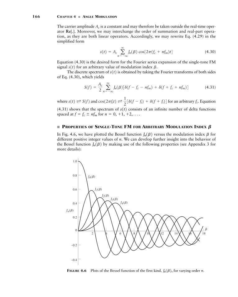
166 CHAPTER 4 � ANGLE MODULATION
The carrier amplitude is a constant and may therefore be taken outside the real-time oper-ator Re[.]. Moreover, we may interchange the order of summation and real-part opera-tion, as they are both linear operators. Accordingly, we may rewrite Eq. (4.29) in thesimplified form
(4.30)
Equation (4.30) is the desired form for the Fourier series expansion of the single-tone FMsignal for an arbitrary value of modulation index
The discrete spectrum of is obtained by taking the Fourier transforms of both sidesof Eq. (4.30), which yields
(4.31)
where and for an arbitrary Equation
(4.31) shows that the spectrum of consists of an infinite number of delta functionsspaced at for
� PROPERTIES OF SINGLE-TONE FM FOR ARBITRARY MODULATION INDEX
In Fig. 4.6, we have plotted the Bessel function versus the modulation index fordifferent positive integer values of n. We can develop further insight into the behavior ofthe Bessel function by making use of the following properties (see Appendix 3 formore details):
Jn1b2bJn1b2B
n � 0, 1, 2, Á .f � fc � nfms1t2
fi .cos12pfit2 L 123d1f � fi2 d1f fi24s1t2 L S1f2
S1f2 �Ac
2 aq
n��qJn1b23d1f � fc � nfm2 d1f fc nfm24
s1t2 b.s1t2s1t2 � Ac a
q
n��qJn1b2 cos32p1fc nfm2t4
Ac
2 4 6 8 10 12 14 16 18
0.2
0.4
0.6
0.8 J0(�)
J1(�)
�
J2(�)J3(�)
J4(�)
Jn(�)
1.0
–0.2
–0.4
0
FIGURE 4.6 Plots of the Bessel function of the first kind, for varying order n.Jn1b2,
4.5 Wide-Band Frequency Modulation 167
1. For different integer (positive and negative) values of n, we have
(4.32)
and
(4.33)
2. For small values of the modulation index we have
(4.34)
3. The equality
(4.35)
holds exactly for arbitrary
Thus using Eqs. (4.31) through (4.35) and the curves of Fig. 4.6, we may make the followingobservations:
1. The spectrum of an FM wave contains a carrier component and an infinite set of sidefrequencies located symmetrically on either side of the carrier at frequency separationsof In this respect, the result is unlike the picture that prevails inAM, since in the latter case a sinusoidal modulating wave gives rise to only one pairof side frequencies.
2. For the special case of small compared with unity, only the Bessel coefficients and have significant values, so that the FM wave is effectively composed of acarrier and a single pair of side-frequencies at This situation corresponds tothe special case of narrow-band FM that was considered in Section 4.4.
3. The amplitude of the carrier component varies with according to That is,unlike an AM wave, the amplitude of the carrier component of an FM wave is depen-dent on the modulation index The physical explanation for this property is thatthe envelope of an FM wave is constant, so that the average power of such a signaldeveloped across a 1-ohm resistor is also constant, as in Eq. (4.8), which is reproducedhere for convenience of presentation:
When the carrier is modulated to generate the FM wave, the power in the side-frequencies may appear only at the expense of the power originally in the carrier,thereby making the amplitude of the carrier component dependent on Note that theaverage power of an FM wave may also be determined from Eq. (4.30), as shown by
(4.36)
Substituting Eq. (4.35) into (4.36), the expression for the average power reducesto Eq. (4.8), and so it should.
Pav
P �12
Ac2 a
q
n��qJn
21b2
b.
Pav �12
Ac2
b.
J01b2.b
fc � fm .J11b2 J01b2b
fm , 2fm , 3fm , Á .
b.
aq
n��qJn
21b2 � 1
J01b2 � 1,
J11b2 �b
2,
Jn1b2 � 0, n � 2
tb,
Jn1b2 � �J�n1b2, for n odd
Jn1b2 � J�n1b2, for n even
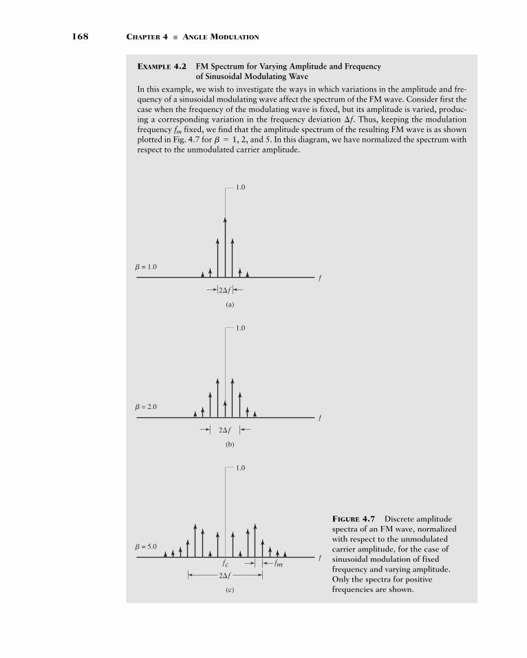
168 CHAPTER 4 � ANGLE MODULATION
EXAMPLE 4.2 FM Spectrum for Varying Amplitude and Frequency of Sinusoidal Modulating Wave
In this example, we wish to investigate the ways in which variations in the amplitude and fre-quency of a sinusoidal modulating wave affect the spectrum of the FM wave. Consider first thecase when the frequency of the modulating wave is fixed, but its amplitude is varied, produc-ing a corresponding variation in the frequency deviation Thus, keeping the modulationfrequency fixed, we find that the amplitude spectrum of the resulting FM wave is as shownplotted in Fig. 4.7 for and 5. In this diagram, we have normalized the spectrum withrespect to the unmodulated carrier amplitude.
b � 1, 2,fm
¢f.
(a)
f
2�f
� = 1.0
1.0
(b)
1.0
f
2�f
� = 2.0
(c)
1.0
ffc fm
2�f
� = 5.0
FIGURE 4.7 Discrete amplitudespectra of an FM wave, normalizedwith respect to the unmodulatedcarrier amplitude, for the case ofsinusoidal modulation of fixedfrequency and varying amplitude.Only the spectra for positivefrequencies are shown.
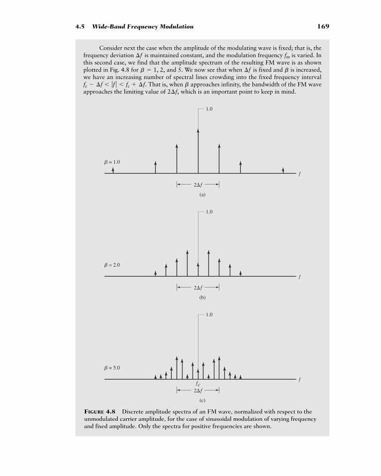
4.5 Wide-Band Frequency Modulation 169
(a)
1.0
f
2�f
� = 1.0
(b)
1.0
f
2�f
� = 2.0
(c)
fc
1.0
f
2�f
� = 5.0
FIGURE 4.8 Discrete amplitude spectra of an FM wave, normalized with respect to theunmodulated carrier amplitude, for the case of sinusoidal modulation of varying frequencyand fixed amplitude. Only the spectra for positive frequencies are shown.
Consider next the case when the amplitude of the modulating wave is fixed; that is, thefrequency deviation is maintained constant, and the modulation frequency is varied. Inthis second case, we find that the amplitude spectrum of the resulting FM wave is as shownplotted in Fig. 4.8 for and 5. We now see that when is fixed and is increased,we have an increasing number of spectral lines crowding into the fixed frequency interval
That is, when approaches infinity, the bandwidth of the FM waveapproaches the limiting value of which is an important point to keep in mind.2¢f,
bfc � ¢f � ƒf ƒ � fc ¢f.
b¢fb � 1, 2,
fm¢f
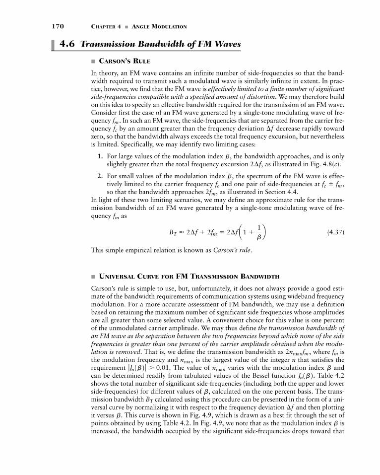
170 CHAPTER 4 � ANGLE MODULATION
4.6 Transmission Bandwidth of FM Waves
� CARSON’S RULE
In theory, an FM wave contains an infinite number of side-frequencies so that the band-width required to transmit such a modulated wave is similarly infinite in extent. In prac-tice, however, we find that the FM wave is effectively limited to a finite number of significantside-frequencies compatible with a specified amount of distortion. We may therefore buildon this idea to specify an effective bandwidth required for the transmission of an FM wave.Consider first the case of an FM wave generated by a single-tone modulating wave of fre-quency In such an FM wave, the side-frequencies that are separated from the carrier fre-quency by an amount greater than the frequency deviation decrease rapidly towardzero, so that the bandwidth always exceeds the total frequency excursion, but neverthelessis limited. Specifically, we may identify two limiting cases:
1. For large values of the modulation index the bandwidth approaches, and is onlyslightly greater than the total frequency excursion as illustrated in Fig. 4.8(c).
2. For small values of the modulation index the spectrum of the FM wave is effec-tively limited to the carrier frequency and one pair of side-frequencies at so that the bandwidth approaches as illustrated in Section 4.4.
In light of these two limiting scenarios, we may define an approximate rule for the trans-mission bandwidth of an FM wave generated by a single-tone modulating wave of fre-quency as
(4.37)
This simple empirical relation is known as Carson’s rule.
� UNIVERSAL CURVE FOR FM TRANSMISSION BANDWIDTH
Carson’s rule is simple to use, but, unfortunately, it does not always provide a good esti-mate of the bandwidth requirements of communication systems using wideband frequencymodulation. For a more accurate assessment of FM bandwidth, we may use a definitionbased on retaining the maximum number of significant side frequencies whose amplitudesare all greater than some selected value. A convenient choice for this value is one percentof the unmodulated carrier amplitude. We may thus define the transmission bandwidth ofan FM wave as the separation between the two frequencies beyond which none of the sidefrequencies is greater than one percent of the carrier amplitude obtained when the modu-lation is removed. That is, we define the transmission bandwidth as where isthe modulation frequency and is the largest value of the integer n that satisfies therequirement The value of varies with the modulation index andcan be determined readily from tabulated values of the Bessel function Table 4.2shows the total number of significant side-frequencies (including both the upper and lowerside-frequencies) for different values of calculated on the one percent basis. The trans-mission bandwidth calculated using this procedure can be presented in the form of a uni-versal curve by normalizing it with respect to the frequency deviation and then plottingit versus This curve is shown in Fig. 4.9, which is drawn as a best fit through the set ofpoints obtained by using Table 4.2. In Fig. 4.9, we note that as the modulation index isincreased, the bandwidth occupied by the significant side-frequencies drops toward that
b
b.¢f
BT
b,
Jn1b2. bnmaxƒJn1b2 ƒ � 0.01.nmax
fm2nmaxfm ,
BT � 2¢f 2fm � 2¢f a1 1bb
fm
2fm,fc � fm ,fc
b,
2¢f,b,
¢ffcfm .
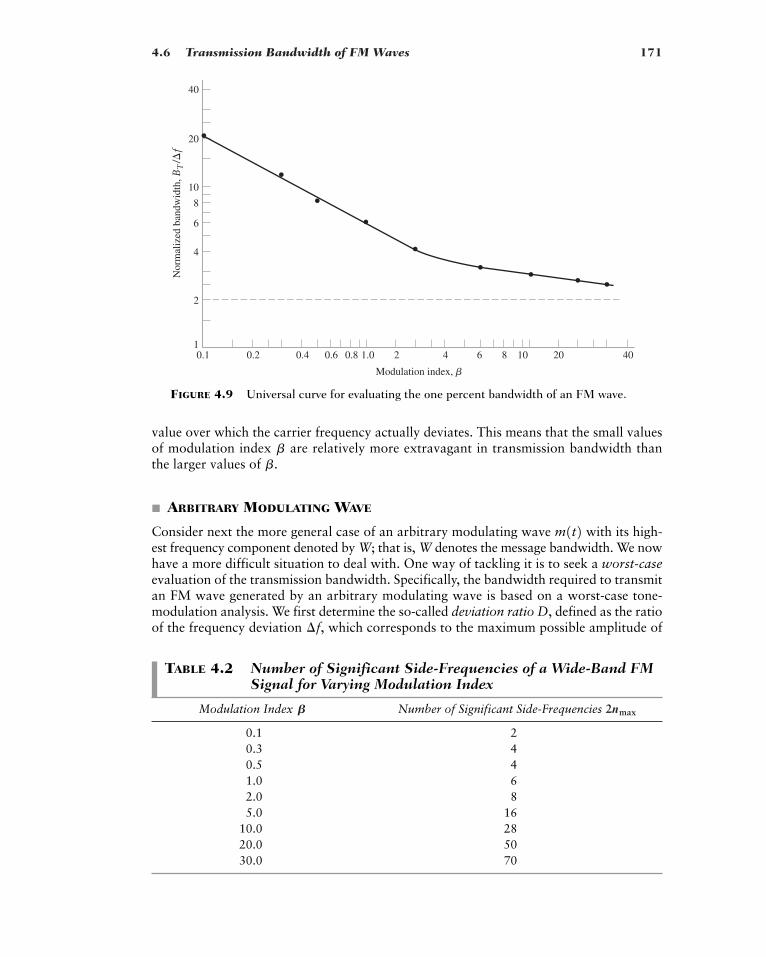
4.6 Transmission Bandwidth of FM Waves 171
0.2 0.4 0.6 0.8 1.0 2
Modulation index, �
Nor
mal
ized
ban
dwid
th, B
T/�
f
4 6 8 10 20 400.1
2
4
6
8
10
20
40
1
FIGURE 4.9 Universal curve for evaluating the one percent bandwidth of an FM wave.
value over which the carrier frequency actually deviates. This means that the small valuesof modulation index are relatively more extravagant in transmission bandwidth thanthe larger values of
� ARBITRARY MODULATING WAVE
Consider next the more general case of an arbitrary modulating wave with its high-est frequency component denoted by W; that is, W denotes the message bandwidth. We nowhave a more difficult situation to deal with. One way of tackling it is to seek a worst-caseevaluation of the transmission bandwidth. Specifically, the bandwidth required to transmitan FM wave generated by an arbitrary modulating wave is based on a worst-case tone-modulation analysis. We first determine the so-called deviation ratio D, defined as the ratioof the frequency deviation which corresponds to the maximum possible amplitude of¢f,
m1t2
b.b
TABLE 4.2 Number of Significant Side-Frequencies of a Wide-Band FMSignal for Varying Modulation Index
Modulation Index Number of Significant Side-Frequencies
0.1 20.3 40.5 41.0 62.0 85.0 16
10.0 2820.0 5030.0 70
2nmaxB
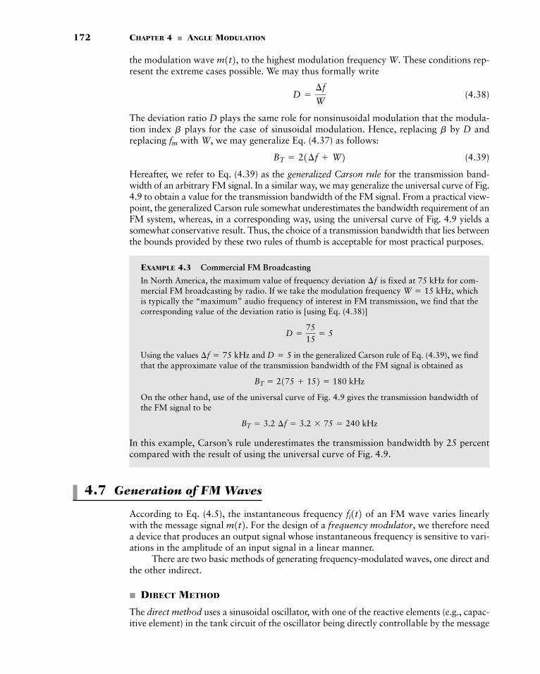
172 CHAPTER 4 � ANGLE MODULATION
the modulation wave to the highest modulation frequency W. These conditions rep-resent the extreme cases possible. We may thus formally write
(4.38)
The deviation ratio D plays the same role for nonsinusoidal modulation that the modula-tion index plays for the case of sinusoidal modulation. Hence, replacing by D andreplacing with W, we may generalize Eq. (4.37) as follows:
(4.39)
Hereafter, we refer to Eq. (4.39) as the generalized Carson rule for the transmission band-width of an arbitrary FM signal. In a similar way, we may generalize the universal curve of Fig.4.9 to obtain a value for the transmission bandwidth of the FM signal. From a practical view-point, the generalized Carson rule somewhat underestimates the bandwidth requirement of anFM system, whereas, in a corresponding way, using the universal curve of Fig. 4.9 yields asomewhat conservative result. Thus, the choice of a transmission bandwidth that lies betweenthe bounds provided by these two rules of thumb is acceptable for most practical purposes.
EXAMPLE 4.3 Commercial FM Broadcasting
In North America, the maximum value of frequency deviation is fixed at 75 kHz for com-mercial FM broadcasting by radio. If we take the modulation frequency whichis typically the “maximum” audio frequency of interest in FM transmission, we find that thecorresponding value of the deviation ratio is [using Eq. (4.38)]
Using the values and in the generalized Carson rule of Eq. (4.39), we findthat the approximate value of the transmission bandwidth of the FM signal is obtained as
On the other hand, use of the universal curve of Fig. 4.9 gives the transmission bandwidth ofthe FM signal to be
In this example, Carson’s rule underestimates the transmission bandwidth by 25 percentcompared with the result of using the universal curve of Fig. 4.9.
4.7 Generation of FM Waves
According to Eq. (4.5), the instantaneous frequency of an FM wave varies linearlywith the message signal For the design of a frequency modulator, we therefore needa device that produces an output signal whose instantaneous frequency is sensitive to vari-ations in the amplitude of an input signal in a linear manner.
There are two basic methods of generating frequency-modulated waves, one direct andthe other indirect.
� DIRECT METHOD
The direct method uses a sinusoidal oscillator, with one of the reactive elements (e.g., capac-itive element) in the tank circuit of the oscillator being directly controllable by the message
m1t2. fi1t2
BT � 3.2 ¢f � 3.2 75 � 240 kHz
BT � 2175 152 � 180 kHz
D � 5¢f � 75 kHz
D �7515
� 5
W � 15 kHz,¢f
BT � 21¢f W2fm
bb
D �¢f
W
m1t2,
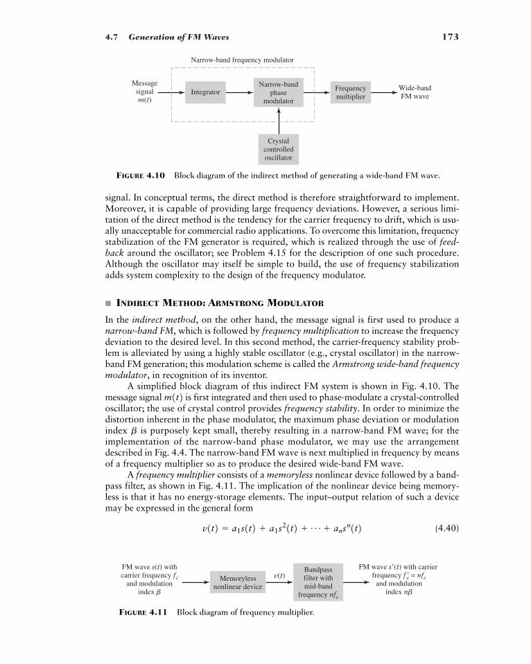
4.7 Generation of FM Waves 173
signal. In conceptual terms, the direct method is therefore straightforward to implement.Moreover, it is capable of providing large frequency deviations. However, a serious limi-tation of the direct method is the tendency for the carrier frequency to drift, which is usu-ally unacceptable for commercial radio applications. To overcome this limitation, frequencystabilization of the FM generator is required, which is realized through the use of feed-back around the oscillator; see Problem 4.15 for the description of one such procedure.Although the oscillator may itself be simple to build, the use of frequency stabilizationadds system complexity to the design of the frequency modulator.
� INDIRECT METHOD: ARMSTRONG MODULATOR
In the indirect method, on the other hand, the message signal is first used to produce anarrow-band FM, which is followed by frequency multiplication to increase the frequencydeviation to the desired level. In this second method, the carrier-frequency stability prob-lem is alleviated by using a highly stable oscillator (e.g., crystal oscillator) in the narrow-band FM generation; this modulation scheme is called the Armstrong wide-band frequencymodulator, in recognition of its inventor.
A simplified block diagram of this indirect FM system is shown in Fig. 4.10. Themessage signal is first integrated and then used to phase-modulate a crystal-controlledoscillator; the use of crystal control provides frequency stability. In order to minimize thedistortion inherent in the phase modulator, the maximum phase deviation or modulationindex is purposely kept small, thereby resulting in a narrow-band FM wave; for theimplementation of the narrow-band phase modulator, we may use the arrangementdescribed in Fig. 4.4. The narrow-band FM wave is next multiplied in frequency by meansof a frequency multiplier so as to produce the desired wide-band FM wave.
A frequency multiplier consists of a memoryless nonlinear device followed by a band-pass filter, as shown in Fig. 4.11. The implication of the nonlinear device being memory-less is that it has no energy-storage elements. The input–output relation of such a devicemay be expressed in the general form
(4.40)v1t2 � a1s1t2 a1s21t2 Á ansn1t2
b
m1t2
Wide-bandFM wave
Frequencymultiplier
Messagesignalm(t)
IntegratorNarrow-band
phasemodulator
Narrow-band frequency modulator
Crystalcontrolledoscillator
FIGURE 4.10 Block diagram of the indirect method of generating a wide-band FM wave.
FM wave s�(t) with carrier frequency f �c = nfc
and modulationindex n�
FM wave s(t) withcarrier frequency fc
and modulationindex �
v(t)Memorylessnonlinear device
Bandpassfilter withmid-band
frequency nfc
FIGURE 4.11 Block diagram of frequency multiplier.
174 CHAPTER 4 � ANGLE MODULATION
where are coefficients determined by the operating point of the device, andn is the highest order of nonlinearity. In other words, the memoryless nonlinear device isan nth power-law device.
The input is an FM wave defined by
(4.41)
where the instantaneous frequency is
(4.42)
Suppose that (1) the mid-band frequency of the bandpass filter in Fig. 4.11 is set equal towhere is the carrier frequency of the incoming FM wave and (2) the bandpass
filter is designed to have a bandwidth equal to n times the transmission bandwidth of In Problem 4.24 dealing with nonlinear effects in FM systems, we address the spectral con-tributions of such nonlinear terms as the second- and third-order terms in the input–out-put relation of Eq. (4.40). For now it suffices to say that after bandpass filtering of thenonlinear device’s output we have a new FM wave defined by
(4.43)
whose instantaneous frequency is
(4.44)
Thus, comparing Eq. (4.44) with (4.42), we see that the nonlinear subsystem of Fig. 4.11acts as a frequency multiplier with and The frequency multiplicationratio n is determined by the highest power n in the input–output relation of Eq. (4.40), char-acterizing the memoryless nonlinear device.
4.8 Demodulation of FM Signals
Frequency demodulation is the process by means of which the original message signal isrecovered from an incoming FM wave. In other words, frequency demodulation is theinverse of frequency modulation. With the frequency modulator being a device that pro-duces an output signal whose instantaneous frequency varies linearly with the amplitudeof the input message signal, it follows that for frequency demodulation we need a devicewhose output amplitude is sensitive to variations in the instantaneous frequency of theinput FM wave in a linear manner too.
In what follows, we describe two devices for frequency demodulation. One device,called a frequency discriminator, relies on slope detection followed by envelope detection.The other device, called a phase-locked loop, performs frequency demodulation in a some-what indirect manner.
� FREQUENCY DISCRIMINATOR
Recall that the FM signal is given by
s1t2 � Ac cosa2pfct 2pkfLt
0m1t2 dtb
kfœ � nkf.fc
œ � nfc
f iœ1t2 � nfc nkf m1t2
s�1t2 � Ac cos c2pfc�t 2pk�fLt
0m1t2 dt d
v1t2,
s1t2.s1t2,fcnfc,
fi1t2 � fc kf m1t2
s1t2 � Ac cos c2pfct 2pkfLt
0m1t2 dt d
s1t2a1, a2, Á , an
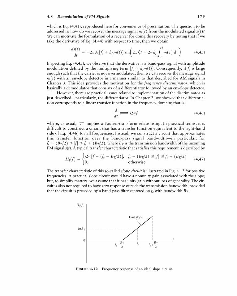
4.8 Demodulation of FM Signals 175
which is Eq. (4.41), reproduced here for convenience of presentation. The question to beaddressed is: how do we recover the message signal from the modulated signal We can motivate the formulation of a receiver for doing this recovery by noting that if wetake the derivative of Eq. (4.44) with respect to time, then we obtain
(4.45)
Inspecting Eq. (4.45), we observe that the derivative is a band-pass signal with amplitudemodulation defined by the multiplying term Consequently, if is largeenough such that the carrier is not overmodulated, then we can recover the message signal
with an envelope detector in a manner similar to that described for AM signals inChapter 3. This idea provides the motivation for the frequency discriminator, which isbasically a demodulator that consists of a differentiator followed by an envelope detector.
However, there are practical issues related to implementation of the discriminator asjust described—particularly, the differentiator. In Chapter 2, we showed that differentia-tion corresponds to a linear transfer function in the frequency domain; that is,
(4.46)
where, as usual, implies a Fourier-transform relationship. In practical terms, it isdifficult to construct a circuit that has a transfer function equivalent to the right-handside of Eq. (4.46) for all frequencies. Instead, we construct a circuit that approximatesthis transfer function over the band-pass signal bandwidth—in particular, for
where is the transmission bandwidth of the incomingFM signal s(t). A typical transfer characteristic that satisfies this requirement is described by
(4.47)
The transfer characteristic of this so-called slope circuit is illustrated in Fig. 4.12 for positivefrequencies. A practical slope circuit would have a nonunity gain associated with the slope;but, to simplify matters, we assume that it has unity gain without loss of generality. The cir-cuit is also not required to have zero response outside the transmission bandwidth, providedthat the circuit is preceded by a band-pass filter centered on with bandwidth BT .fc
H11f2 � b j2p3f � 1fc � BT>224, fc � 1BT>22 � ƒf ƒ � fc 1BT>220, otherwise
BTfc � 1BT>22 � ƒf ƒ � fc 1BT>22,
L
ddt
Δ j2pf
m1t2fc3fc kfm1t24.
ds1t2dt
� �2pAc3fc kf m1t24 sina2pfct 2pkfLt
0m1t2 dtb
s1t2?m1t2
H1(f )
ffcfc
0
Unit slope
j�BT
—––2
BT fc —–+2
BT
FIGURE 4.12 Frequency response of an ideal slope circuit.
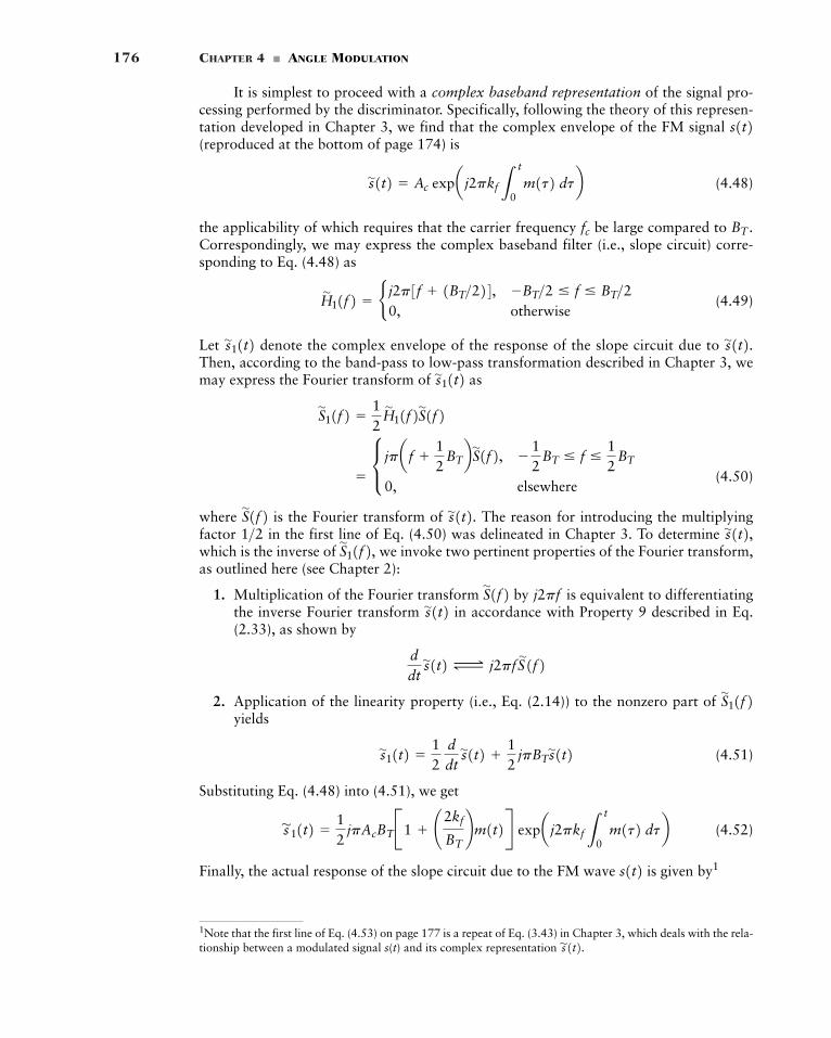
176 CHAPTER 4 � ANGLE MODULATION
1Note that the first line of Eq. (4.53) on page 177 is a repeat of Eq. (3.43) in Chapter 3, which deals with the rela-tionship between a modulated signal s(t) and its complex representation s
'1t2.
It is simplest to proceed with a complex baseband representation of the signal pro-cessing performed by the discriminator. Specifically, following the theory of this represen-tation developed in Chapter 3, we find that the complex envelope of the FM signal (reproduced at the bottom of page 174) is
(4.48)
the applicability of which requires that the carrier frequency be large compared to Correspondingly, we may express the complex baseband filter (i.e., slope circuit) corre-sponding to Eq. (4.48) as
(4.49)
Let denote the complex envelope of the response of the slope circuit due to Then, according to the band-pass to low-pass transformation described in Chapter 3, wemay express the Fourier transform of as
(4.50)
where is the Fourier transform of The reason for introducing the multiplyingfactor in the first line of Eq. (4.50) was delineated in Chapter 3. To determine which is the inverse of we invoke two pertinent properties of the Fourier transform,as outlined here (see Chapter 2):
1. Multiplication of the Fourier transform by is equivalent to differentiatingthe inverse Fourier transform in accordance with Property 9 described in Eq.(2.33), as shown by
2. Application of the linearity property (i.e., Eq. (2.14)) to the nonzero part of yields
(4.51)
Substituting Eq. (4.48) into (4.51), we get
(4.52)
Finally, the actual response of the slope circuit due to the FM wave is given by1s1t2s'
11t2 �12
jpAcBTB1 ¢2kf
BT≤m1t2R expa j2pkfL
t
0m1t2 dtb
s'
11t2 �12
ddt
s'1t2
12
jpBTs'1t2
S'
11f2ddt
s'1t2 Δ j2pfS
'1f2s'1t2 j2pfS
'1f2S'
11f2, s'1t2,1>2 s
'1t2.S'1f2
�c jpaf
12
BTbS'1f2, �12
BT � f �12
BT
0, elsewhere
S'
11f2 �12
H'
11f2S'1f2s'
11t2s'1t2.s
'11t2
H'
11f2 � b j2p3f 1BT>224, �BT>2 � f � BT>20, otherwise
BT .fc
s'1t2 � Ac expa j2pkfL
t
0m1t2 dtb
s1t2
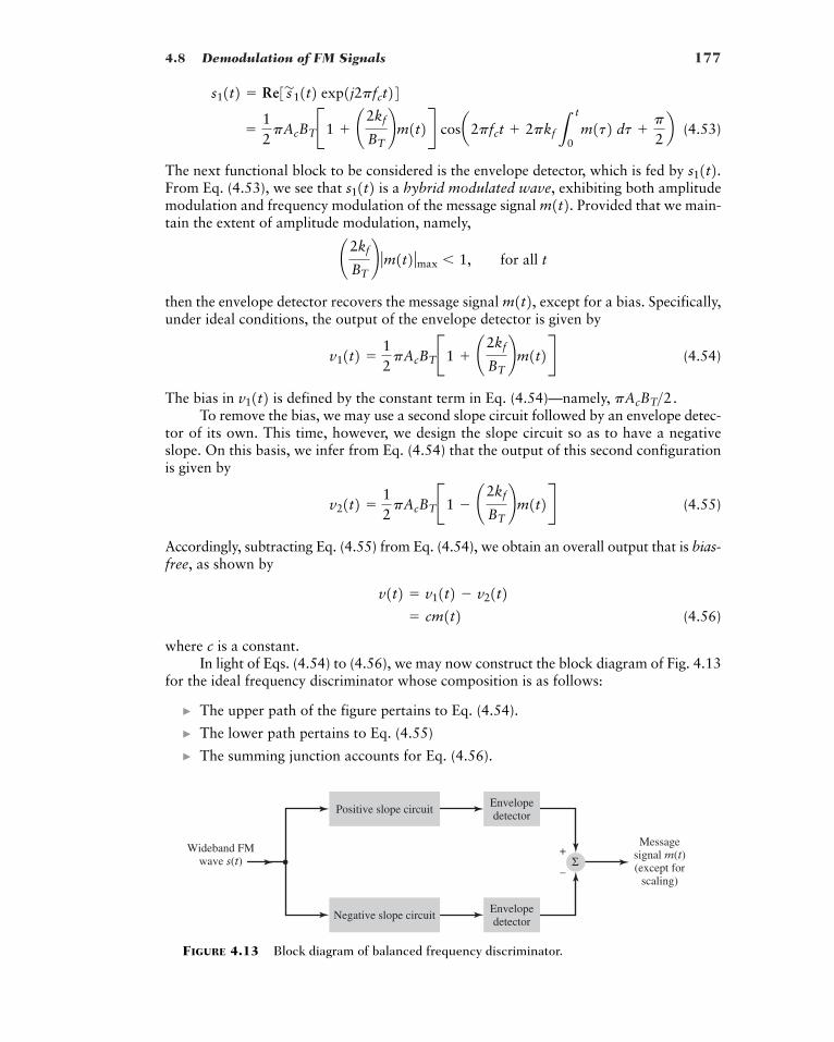
4.8 Demodulation of FM Signals 177
(4.53)
The next functional block to be considered is the envelope detector, which is fed by From Eq. (4.53), we see that is a hybrid modulated wave, exhibiting both amplitudemodulation and frequency modulation of the message signal Provided that we main-tain the extent of amplitude modulation, namely,
then the envelope detector recovers the message signal except for a bias. Specifically,under ideal conditions, the output of the envelope detector is given by
(4.54)
The bias in is defined by the constant term in Eq. (4.54)—namely, To remove the bias, we may use a second slope circuit followed by an envelope detec-
tor of its own. This time, however, we design the slope circuit so as to have a negativeslope. On this basis, we infer from Eq. (4.54) that the output of this second configurationis given by
(4.55)
Accordingly, subtracting Eq. (4.55) from Eq. (4.54), we obtain an overall output that is bias-free, as shown by
(4.56)
where c is a constant.In light of Eqs. (4.54) to (4.56), we may now construct the block diagram of Fig. 4.13
for the ideal frequency discriminator whose composition is as follows:
� The upper path of the figure pertains to Eq. (4.54).
� The lower path pertains to Eq. (4.55)
� The summing junction accounts for Eq. (4.56).
� cm1t2v1t2 � v11t2 � v21t2
v21t2 �12pAcBTB1 � ¢2kf
BT≤m1t2R
pAcBT>2.v11t2v11t2 �
12pAcBTB1 ¢2kf
BT≤m1t2R
m1t2,¢2kf
BT≤ ƒm1t2 ƒmax � 1, for all t
m1t2.s11t2 s11t2.�
12pAcBTB1 ¢2kf
BT≤m1t2R cosa2pfct 2pkfL
t
0m1t2 dt
p
2b
s11t2 � Re3s'11t2 exp1j2pfct24
Wideband FMwave s(t)
Messagesignal m(t)(except for
scaling)
Positive slope circuit
Negative slope circuit
Envelopedetector
Envelopedetector
+
–Σ
FIGURE 4.13 Block diagram of balanced frequency discriminator.
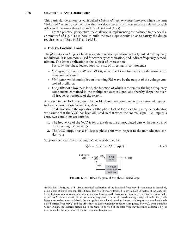
178 CHAPTER 4 � ANGLE MODULATION
2In Haykin (1994), pp. 178–180, a practical realization of the balanced frequency discriminator is described,using a pair of highly resonant RLC filters. The two filters are designed to have a high Q-factor. The quality fac-tor or Q-factor of a resonant filter is a measure of how sharp the frequency response of the filter is; it is formallydefined as times the ratio of the maximum energy stored in the filter to the energy dissipated in the filter, bothbeing measured on a per cycle basis. For the application at hand, one filter is tuned to a frequency above the unmod-ulated carrier frequency and the other filter is correspondingly tuned to a frequency below By making theQ-factor high, the linearity pertaining to the required portion of the total frequency response, centered on isdetermined by the separation of the two resonant frequencies.
fc ,fc .fc
2p
This particular detection system is called a balanced frequency discriminator, where the term“balanced” refers to the fact that the two slope circuits of the system are related to eachother in the manner described in Eqs. (4.54) and (4.55).
From a practical perspective, the challenge in implementing the balanced frequency dis-criminator2 of Fig. 4.13 is how to build the two slope circuits so as to satisfy the designrequirements of Eqs. (4.54) and (4.55).
� PHASE-LOCKED LOOP
The phase-locked loop is a feedback system whose operation is closely linked to frequencymodulation. It is commonly used for carrier synchronization, and indirect frequency demod-ulation. The latter application is the subject of interest here.
Basically, the phase-locked loop consists of three major components:
� Voltage-controlled oscillator (VCO), which performs frequency modulation on itsown control signal.
� Multiplier, which multiplies an incoming FM wave by the output of the voltage-con-trolled oscillator.
� Loop filter of a low-pass kind, the function of which is to remove the high-frequencycomponents contained in the multiplier’s output signal and thereby shape the over-all frequency response of the system.
As shown in the block diagram of Fig. 4.14, these three components are connected togetherto form a closed-loop feedback system.
To demonstrate the operation of the phase-locked loop as a frequency demodulator,we assume that the VCO has been adjusted so that when the control signal (i.e., input) iszero, two conditions are satisfied:
1. The frequency of the VCO is set precisely at the unmodulated carrier frequency ofthe incoming FM wave
2. The VCO output has a 90-degree phase-shift with respect to the unmodulated car-rier wave.
Suppose then that the incoming FM wave is defined by
(4.57)s1t2 � Ac sin32pfct f11t24
s1t2. fc
v(t)e(t)
r(t)
Loopfilter
Voltagecontrolledoscillator
FM waves(t)
FIGURE 4.14 Block diagram of the phase-locked loop.
4.8 Demodulation of FM Signals 179
where is the carrier amplitude. By definition, the angle is related to the messagesignal by the integral
(4.58)
where is the frequency-sensitivity factor of the frequency modulator responsible for thegeneration of Correspondingly, in accordance with points (1) and (2) on page 178, wedefine the FM wave produced by the VCO as
(4.59)
where is the amplitude. The angle is related to the control signal of the VCOby the integral
(4.60)
where is the frequency-sensitivity factor of the VCO.The function of the feedback loop acting around the VCO is to adjust the angle
so that it equals thereby setting the stage for frequency demodulation. To delve moredeeply into this function and how it can arise, we need to develop a model for the phase-locked loop, as described next.
To this end, we first note that multiplication of the incoming FM wave by the locallygenerated FM wave produces two components (except for the scaling factor ):
1. A high-frequency component, which is defined by the double-frequency term—namely,
where is the multiplier gain.2. A low-frequency component, which is defined by the difference-frequency term—
namely,
� Drill Problem 4.6 Using a well-known trigonometric identity involving the product ofthe sine of an angle and the cosine of another angle, demonstrate the two results just describedunder points 1 and 2. �
With the loop-filter designed to suppress the high-frequency components in the mul-tiplier’s output, we may henceforth discard the double-frequency term. Doing this, we mayreduce the signal applied to the loop filter to
(4.61)
where is the phase error defined by
(4.62)
When the phase error is zero, the phase-locked loop is said to be in phase-lock.It is said to be near-phase-lock when the phase error is small compared with oneradian, under which condition we may use the approximation
sin3fe1t24 � fe1t2fe1t2fe1t2
� f11t2 � 2pkvLt
0v1t2 dt
fe1t2 � f11t2 � f21t2fe1t2
e1t2 � kmAcAv sin3fe1t24
kmAcAv sin3f11t2 � f21t24
km
kmAcAv sin34pfct f11t2 f21t241>2r1t2 s1t2
f11t2, f21t2kv
f21t2 � 2pkvLt
0v1t2 dt
v1t2f21t2Av
r1t2 � Av cos32pfct f21t24s1t2.kf
f11t2 � 2pkfLt
0m1t2 dt
m1t2 f11t2Ac
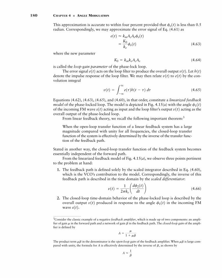
180 CHAPTER 4 � ANGLE MODULATION
3Consider the classic example of a negative feedback amplifier, which is made up of two components: an ampli-fier of gain in the forward path and a network of gain in the feedback path. The closed-loop gain of the ampli-fier is defined by
The product term in the denominator is the open-loop gain of the feedback amplifier. When is large com-pared with unity, the formula for A is effectively determined by the inverse of as shown by
A �1b
b,mbmb
A �m
1 mb
bm
This approximation is accurate to within four percent provided that is less than 0.5radian. Correspondingly, we may approximate the error signal of Eq. (4.61) as
(4.63)
where the new parameter
(4.64)
is called the loop-gain parameter of the phase-lock loop.The error signal acts on the loop filter to produce the overall output Let
denote the impulse response of the loop filter. We may then relate to by the con-volution integral
(4.65)
Equations (4.62), (4.63), (4.65), and (4.60), in that order, constitute a linearized feedbackmodel of the phase-locked loop. The model is depicted in Fig. 4.15(a) with the angle of the incoming FM wave acting as input and the loop filter’s output acting as theoverall output of the phase-locked loop.
From linear feedback theory, we recall the following important theorem:3
When the open-loop transfer function of a linear feedback system has a largemagnitude compared with unity for all frequencies, the closed-loop transferfunction of the system is effectively determined by the inverse of the transfer func-tion of the feedback path.
Stated in another way, the closed-loop transfer function of the feedback system becomesessentially independent of the forward path.
From the linearized feedback model of Fig. 4.15(a), we observe three points pertinentto the problem at hand:
1. The feedback path is defined solely by the scaled integrator described in Eq. (4.60),which is the VCO’s contribution to the model. Correspondingly, the inverse of thisfeedback path is described in the time domain by the scaled differentiator:
(4.66)
2. The closed-loop time-domain behavior of the phase-locked loop is described by theoverall output produced in response to the angle in the incoming FM wave s1t2. f11t2v1t2
v1t2 �1
2pkv¢df21t2
dt≤
v1t2s1t2 f11t2
v1t2 � Lq
�qe1t2h1t � t2 dt
e1t2v1t2 h1t2v1t2.e1t2K0 � kmkvAcAv
�K0
kvfe1t2
e1t2 � kmAcAvfe1t2fe1t2
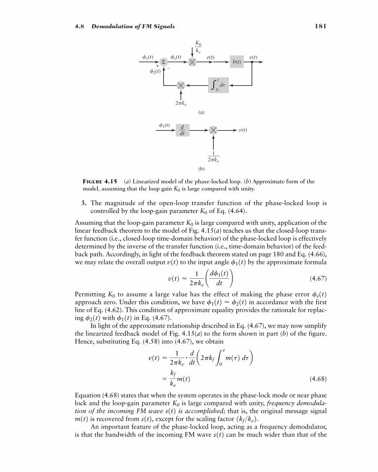
4.8 Demodulation of FM Signals 181
(a)
(b)
v(t)�1(t)
12�kv—–––
ddt—
h(t)e(t) v(t)
2�kv
�2(t)
�1(t) �e(t)
+ –Σ
d�
K0
kv—–
t
0�
FIGURE 4.15 (a) Linearized model of the phase-locked loop. (b) Approximate form of themodel, assuming that the loop gain is large compared with unity.K0
3. The magnitude of the open-loop transfer function of the phase-locked loop iscontrolled by the loop-gain parameter of Eq. (4.64).
Assuming that the loop-gain parameter is large compared with unity, application of thelinear feedback theorem to the model of Fig. 4.15(a) teaches us that the closed-loop trans-fer function (i.e., closed-loop time-domain behavior) of the phase-locked loop is effectivelydetermined by the inverse of the transfer function (i.e., time-domain behavior) of the feed-back path. Accordingly, in light of the feedback theorem stated on page 180 and Eq. (4.66),we may relate the overall output to the input angle by the approximate formula
(4.67)
Permitting to assume a large value has the effect of making the phase error approach zero. Under this condition, we have in accordance with the firstline of Eq. (4.62). This condition of approximate equality provides the rationale for replac-ing with in Eq. (4.67).
In light of the approximate relationship described in Eq. (4.67), we may now simplifythe linearized feedback model of Fig. 4.15(a) to the form shown in part (b) of the figure.Hence, substituting Eq. (4.58) into (4.67), we obtain
(4.68)
Equation (4.68) states that when the system operates in the phase-lock mode or near phaselock and the loop-gain parameter is large compared with unity, frequency demodula-tion of the incoming FM wave is accomplished; that is, the original message signal
is recovered from except for the scaling factor An important feature of the phase-locked loop, acting as a frequency demodulator,
is that the bandwidth of the incoming FM wave can be much wider than that of thes1t21kf>kv2.s1t2,m1t2 s1t2K0
�kf
kvm1t2
v1t2 �1
2pkv
# ddta2pkfL
t
0m1t2 dtb
f11t2f21t2f11t2 � f21t2 fe1t2K0
v1t2 �1
2pkv¢df11t2
dt≤f11t2v1t2
K0
K0
182 CHAPTER 4 � ANGLE MODULATION
loop filter characterized by the transfer function —that is, the Fourier transform of theloop filter’s impulse response The transfer function of the loop filter can andtherefore should be restricted to the baseband (i.e., the original frequency band occupiedby the message signal). Then the control signal of the VCO—namely, —has the band-width of the baseband (message) signal whereas the VCO output is a wide-bandfrequency-modulated wave whose instantaneous frequency tracks the variations in theinstantaneous frequency of the incoming FM wave due to Here we are merelyrestating the fact that the bandwidth of a wide-band FM wave is much larger than thebandwidth of the message signal responsible for its generation.
The complexity of the phase-locked loop is determined by the transfer function of the loop filter. The simplest form of a phase-locked loop is obtained by setting that is, there is no loop filter, in which case the phase-locked loop is referred to as a first-order phase-locked loop. For higher order loops, the transfer function assumes amore complex frequency-dependent form.
A major limitation of a first-order phase-locked loop is that the loop-gain parametercontrols both the loop bandwidth as well as the hold-in frequency range of the loop.
The hold-in frequency range refers to the range of frequencies for which the loop remainsin a phase-locked condition with respect to the incoming FM wave. It is for this reason thatdespite its simplicity, a first-order phase-locked loop is seldom used in practice. Rather, therecommended procedure is to use a second-order phase-locked loop, the realization ofwhich is satisfied by using a first-order loop filter; See Problem 4.25.
� Drill Problem 4.7 Using the linearized model of Fig. 4.15(a), show that the model isapproximately governed by the integro-differential equation
Hence, derive the following two approximate results in the frequency domain:
(a)
(b)
where
is the open-loop transfer function. Finally, show that when is large compared with unityfor all frequencies inside the message band, the time-domain version of the formula in part (b)reduces to the approximate form in Eq. (4.68). �
4.9 Theme Example: FM StereoMultiplexing
Stereo multiplexing is a form of frequency-division multiplexing (FDM) designed to trans-mit two separate signals via the same carrier. It is widely used in FM radio broadcasting tosend two different elements of a program (e.g., two different sections of an orchestra, avocalist and an accompanist) so as to give a spatial dimension to its perception by a listenerat the receiving end.
L1f2L1f2 � K0
H1f2jf
V1f2 �jf
kv
L1f21 L1f2 £11f2
£e1f2 �1
1 L1f2 £11f2
dfe1t2dt
2pK0Lq
�qfe1t2h1t � t2 dt �
df11t2dt
K0
H1f2H1f2 � 1;
H1f2m1t2.s1t2
r1t2m1t2, v1t2H1f2h1t2. H1f2
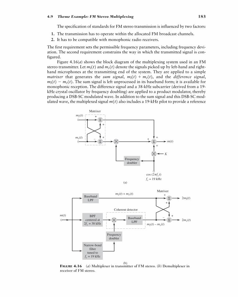
4.9 Theme Example: FM Stereo Multiplexing 183
(a)
(b)
Frequencydoubler
Matrixer
Matrixer
m(t)
cos (2�fct)fc = 19 kHz
K
ml(t)
mr(t)
Σ
Σ
+
+
+ +
+Σ
– +
m(t)
ml(t) + mr(t)
ml(t) – mr(t)2mr(t)
2ml(t)
Coherent detector
Σ+
+
+Σ
–
BasebandLPF
BPFcentered at
2fc = 38 kHz
Narrow-bondfilter
tuned tofc = 19 kHz
BasebandLPF
Frequencydoubler
FIGURE 4.16 (a) Multiplexer in transmitter of FM stereo. (b) Demultiplexer inreceiver of FM stereo.
The specification of standards for FM stereo transmission is influenced by two factors:
1. The transmission has to operate within the allocated FM broadcast channels.2. It has to be compatible with monophonic radio receivers.
The first requirement sets the permissible frequency parameters, including frequency devi-ation. The second requirement constrains the way in which the transmitted signal is con-figured.
Figure 4.16(a) shows the block diagram of the multiplexing system used in an FMstereo transmitter. Let and denote the signals picked up by left-hand and right-hand microphones at the transmitting end of the system. They are applied to a simplematrixer that generates the sum signal, and the difference signal,
The sum signal is left unprocessed in its baseband form; it is available formonophonic reception. The difference signal and a 38-kHz subcarrier (derived from a 19-kHz crystal oscillator by frequency doubling) are applied to a product modulator, therebyproducing a DSB-SC modulated wave. In addition to the sum signal and this DSB-SC mod-ulated wave, the multiplexed signal also includes a 19-kHz pilot to provide a referencem1t2
ml1t2 � mr1t2. ml1t2 mr1t2,mr1t2ml1t2
184 CHAPTER 4 � ANGLE MODULATION
for the coherent detection of the difference signal at the stereo receiver. Thus in accordancewith Fig. 4.16(a), the multiplexed signal is described by
(4.69)
where and K is the amplitude of the pilot tone. The multiplexed signal then frequency-modulates the main carrier to produce the transmitted signal, this frequencymodulation is not shown in Fig. 4.16(a). The pilot is allotted between 8 and 10 percent of thepeak frequency deviation; the amplitude K in Eq. (4.69) is chosen to satisfy this requirement.
At a stereo receiver, first of all the multiplexed signal is recovered by frequencydemodulating the incoming FM wave. Then is applied to the demultiplexing systemshown in Fig. 4.16(b). The individual components of the multiplexed signal are sep-arated by the use of three appropriate filters. The recovered pilot (using a narrow-band fil-ter tuned to 19 kHz) is frequency-doubled to produce the desired 38-kHz subcarrier. Theavailability of this subcarrier enables the coherent detection of the DSB-SC modulatedwave, see the part of Fig. 4.16(b) inside the dashed rectangle. The difference signal
is thereby recovered. The baseband low-pass filter in the top path ofFig. 4.16(b) is designed to pass the sum signal, Finally, the simple matrixerreconstructs the original left-hand signal and right-hand signal except for thescaling factor 2, and applies them to their respective speakers. FM stereophonic receptionis thereby accomplished.
4.10 Summary and Discussion
In Chapter 3, we studied the underlying principles of the first family of continuous-wave (CW)modulation, based on amplitude modulation and its variants. In this chapter, we completed thestudy of the underlying principles of CW modulation, based on angle modulation.
Fundamentally, there are two kinds of angle modulation:
� Phase modulation (PM), where the instantaneous phase of the sinusoidal carrier waveis varied linearly with the message signal.
� Frequency modulation (FM), where the instantaneous frequency of the sinusoidalcarrier wave is varied linearly with the message signal.
These two methods of modulation are closely related in that if we are given one of them,we can derive the other one. For this reason we focused much of the discussion on fre-quency modulation.
Frequency modulation (FM) is typified by the equation
(4.70)
where is the message signal, is the sinusoidal carrier wave, and is thefrequency sensitivity of the modulator. Equation (4.70) is a repeat of Eq. (4.7), reproducedat this point merely for convenience of presentation.
Unlike amplitude modulation, from Eq. (4.70) we see that FM is a nonlinear modu-lation process. Accordingly, the spectral analysis of FM is more difficult than for AM. Nev-ertheless, by studying single-tone FM, we were able to develop a great deal of insight intothe spectral properties of FM. In particular, we derived an empirical rule known as thegeneralized Carson rule for an approximate evaluation of the transmission bandwidth of FM. According to this rule, is controlled by a single parameter: the modulation index
for sinusoidal FM or the deviation ratio D for nonsinusoidal FM.In FM, the carrier amplitude and therefore the transmitted average power is maintained
constant. Herein lies the important advantage of FM over AM in combating the effects of noise
b
BT
BT
kfAc cos12pfct2m1t2s1t2 � Ac cosa2pfct 2pkfL
t
0m1t2 dtb
mr1t2,ml1t2ml1t2 mr1t2.ml1t2 � mr1t2
m1t2m1t2 m1t2
m1t2fc � 19 kHz,
m1t2 � 3ml1t2 mr1t24 3ml � mr1t24 cos14pfct2 K cos12pfct2
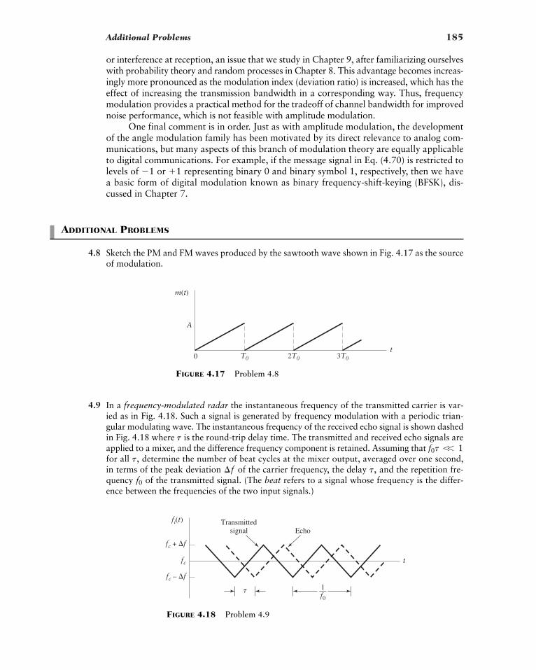
Additional Problems 185
or interference at reception, an issue that we study in Chapter 9, after familiarizing ourselveswith probability theory and random processes in Chapter 8. This advantage becomes increas-ingly more pronounced as the modulation index (deviation ratio) is increased, which has theeffect of increasing the transmission bandwidth in a corresponding way. Thus, frequencymodulation provides a practical method for the tradeoff of channel bandwidth for improvednoise performance, which is not feasible with amplitude modulation.
One final comment is in order. Just as with amplitude modulation, the developmentof the angle modulation family has been motivated by its direct relevance to analog com-munications, but many aspects of this branch of modulation theory are equally applicableto digital communications. For example, if the message signal in Eq. (4.70) is restricted tolevels of or representing binary 0 and binary symbol 1, respectively, then we havea basic form of digital modulation known as binary frequency-shift-keying (BFSK), dis-cussed in Chapter 7.
ADDITIONAL PROBLEMS
4.8 Sketch the PM and FM waves produced by the sawtooth wave shown in Fig. 4.17 as the sourceof modulation.
1�1
4.9 In a frequency-modulated radar the instantaneous frequency of the transmitted carrier is var-ied as in Fig. 4.18. Such a signal is generated by frequency modulation with a periodic trian-gular modulating wave. The instantaneous frequency of the received echo signal is shown dashedin Fig. 4.18 where is the round-trip delay time. The transmitted and received echo signals areapplied to a mixer, and the difference frequency component is retained. Assuming that for all determine the number of beat cycles at the mixer output, averaged over one second,in terms of the peak deviation of the carrier frequency, the delay and the repetition fre-quency of the transmitted signal. (The beat refers to a signal whose frequency is the differ-ence between the frequencies of the two input signals.)
f0t,¢f
t,f0t V 1
t
m(t)
t0
A
T0 2T0 3T0
FIGURE 4.17 Problem 4.8
fi(t)
tfc
fc + �f
fc – �f
EchoTransmitted
signal
� 1f0––
FIGURE 4.18 Problem 4.9
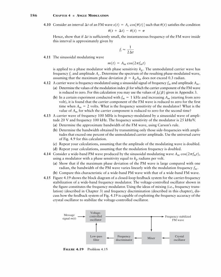
186 CHAPTER 4 � ANGLE MODULATION
Messagesignal m(t)
Voltage-controlledoscillator
Low-passfilter
Frequencydiscriminator
Frequency-stabilizedFM wave
MixerCrystal
oscillator
FIGURE 4.19 Problem 4.15
4.10 Consider an interval of an FM wave such that satisfies the condition
Hence, show that if is sufficiently small, the instantaneous frequency of the FM wave insidethis interval is approximately given by
4.11 The sinusoidal modulating wave
is applied to a phase modulator with phase sensitivity The unmodulated carrier wave hasfrequency and amplitude Determine the spectrum of the resulting phase-modulated wave,assuming that the maximum phase deviation does not exceed 0.3 radian.
4.12 A carrier wave is frequency-modulated using a sinusoidal signal of frequency and amplitude (a) Determine the values of the modulation index for which the carrier component of the FM wave
is reduced to zero. For this calculation you may use the values of given in Appendix 3.(b) In a certain experiment conducted with and increasing (starting from zero
volt), it is found that the carrier component of the FM wave is reduced to zero for the firsttime when What is the frequency sensitivity of the modulator? What is thevalue of for which the carrier component is reduced to zero for the second time?
4.13 A carrier wave of frequency 100 MHz is frequency-modulated by a sinusoidal wave of ampli-tude 20 V and frequency 100 kHz. The frequency sensitivity of the modulator is 25 kHz/V.(a) Determine the approximate bandwidth of the FM wave, using Carson’s rule.(b) Determine the bandwidth obtained by transmitting only those side-frequencies with ampli-
tudes that exceed one percent of the unmodulated carrier amplitude. Use the universal curveof Fig. 4.9 for this calculation.
(c) Repeat your calculations, assuming that the amplitude of the modulating wave is doubled.(d) Repeat your calculations, assuming that the modulation frequency is doubled.
4.14 Consider a wide-band PM wave produced by the sinusoidal modulating wave using a modulator with a phase sensitivity equal to radians per volt.(a) Show that if the maximum phase deviation of the PM wave is large compared with one
radian, the bandwidth of the PM wave varies linearly with the modulation frequency (b) Compare this characteristic of a wide-band PM wave with that of a wide-band FM wave.
4.15 Figure 4.19 shows the block diagram of a closed-loop feedback system for the carrier-frequencystabilization of a wide-band frequency modulator. The voltage-controlled oscillator shown inthe figure constitutes the frequency modulator. Using the ideas of mixing (i.e., frequency trans-lation) (described in Chapter 3) and frequency discrimination (described in this chapter), dis-cuss how the feedback system of Fig. 4.19 is capable of exploiting the frequency accuracy of thecrystal oscillator to stabilize the voltage-controlled oscillator.
fm .
kp
Am cos12pfmt2,
Am
Am � 2 volts.
Amfm � 1 kHzJ01b2b
Am .fm
b � kpAm
Ac .fckp .
m1t2 � Am cos12pfmt2fi �
12¢t
¢t
u1t ¢t2 � u1t2 � p
u1t2s1t2 � Ac cos3u1t24¢t
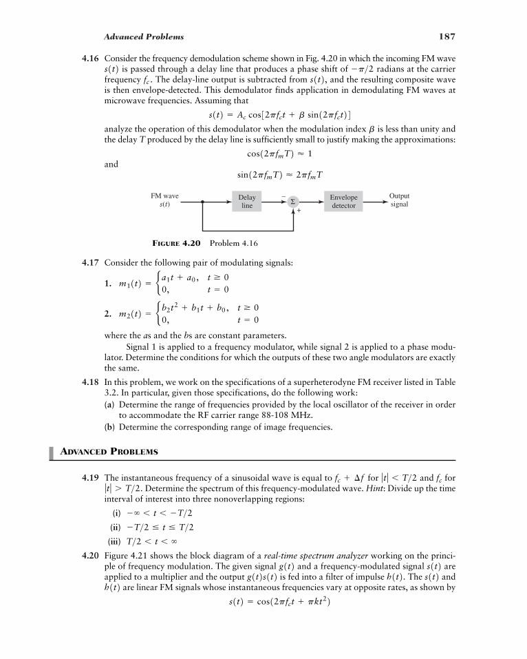
Advanced Problems 187
4.16 Consider the frequency demodulation scheme shown in Fig. 4.20 in which the incoming FM waveis passed through a delay line that produces a phase shift of radians at the carrier
frequency The delay-line output is subtracted from and the resulting composite waveis then envelope-detected. This demodulator finds application in demodulating FM waves atmicrowave frequencies. Assuming that
analyze the operation of this demodulator when the modulation index is less than unity andthe delay T produced by the delay line is sufficiently small to justify making the approximations:
andsin12pfmT2 � 2pfmT
cos12pfmT2 � 1
b
s1t2 � Ac cos32pfct b sin12pfct24
s1t2,fc .�p>2s1t2
4.17 Consider the following pair of modulating signals:
1.
2.
where the as and the bs are constant parameters.Signal 1 is applied to a frequency modulator, while signal 2 is applied to a phase modu-
lator. Determine the conditions for which the outputs of these two angle modulators are exactlythe same.
4.18 In this problem, we work on the specifications of a superheterodyne FM receiver listed in Table3.2. In particular, given those specifications, do the following work:(a) Determine the range of frequencies provided by the local oscillator of the receiver in order
to accommodate the RF carrier range 88-108 MHz.(b) Determine the corresponding range of image frequencies.
ADVANCED PROBLEMS
4.19 The instantaneous frequency of a sinusoidal wave is equal to for and forDetermine the spectrum of this frequency-modulated wave. Hint: Divide up the time
interval of interest into three nonoverlapping regions:
(i)
(ii)
(iii)
4.20 Figure 4.21 shows the block diagram of a real-time spectrum analyzer working on the princi-ple of frequency modulation. The given signal and a frequency-modulated signal areapplied to a multiplier and the output is fed into a filter of impulse The and
are linear FM signals whose instantaneous frequencies vary at opposite rates, as shown by
s1t2 � cos12pfct pkt22h1t2 s1t2h1t2.g1t2s1t2 s1t2g1t2
T>2 � t � �
�T>2 � t � T>2�� � t � �T>2
ƒ t ƒ � T>2.fcƒ t ƒ � T>2fc ¢f
m21t2 � b b2t2 b1t b0 , t � 00, t � 0
m11t2 � b a1t a0 , t � 00, t � 0
Delayline
Envelopedetector
FM waves(t)
Outputsignal
–
+Σ
FIGURE 4.20 Problem 4.16
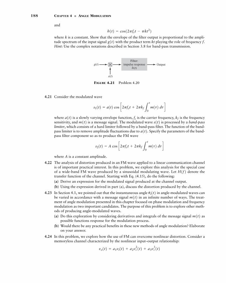
188 CHAPTER 4 � ANGLE MODULATION
and
where k is a constant. Show that the envelope of the filter output is proportional to the ampli-tude spectrum of the input signal with the product term kt playing the role of frequency Hint: Use the complex notations described in Section 3.8 for band-pass transmission.
f.g1t2h1t2 � cos12pfct � pkt22
Filter:impulse response
h(t)Outputg(t)
s(t)
FIGURE 4.21 Problem 4.20
4.21 Consider the modulated wave
where is a slowly varying envelope function, is the carrier frequency, is the frequencysensitivity, and is a message signal. The modulated wave is processed by a band-passlimiter, which consists of a hard limiter followed by a band-pass filter. The function of the band-pass limiter is to remove amplitude fluctuations due to Specify the parameters of the band-pass filter component so as to produce the FM wave
where A is a constant amplitude.
4.22 The analysis of distortion produced in an FM wave applied to a linear communication channelis of important practical interest. In this problem, we explore this analysis for the special caseof a wide-band FM wave produced by a sinusoidal modulating wave. Let denote thetransfer function of the channel. Starting with Eq. (4.15), do the following:(a) Derive an expression for the modulated signal produced at the channel output.(b) Using the expression derived in part (a), discuss the distortion produced by the channel.
4.23 In Section 4.1, we pointed out that the instantaneous angle in angle-modulated waves canbe varied in accordance with a message signal in an infinite number of ways. The treat-ment of angle modulation presented in this chapter focused on phase modulation and frequencymodulation as two important candidates. The purpose of this problem is to explore other meth-ods of producing angle-modulated waves.(a) Do this exploration by considering derivatives and integrals of the message signal as
possible functions response for the modulation process.(b) Would there be any practical benefits in these new methods of angle modulation? Elaborate
on your answer.
4.24 In this problem, we explore how the use of FM can overcome nonlinear distortion. Consider amemoryless channel characterized by the nonlinear input–output relationship:
vo1t2 � a1vi1t2 a2vi21t2 a3vi
31t2
m1t2
m1t2 ui1t2
H1f2
s21t2 � A cos c2pfct 2pkfLt
0m1t2 dt d
a1t2.s1t2m1t2 kffca1t2
s11t2 � a1t2 cos c2pfct 2pkfLt
0m1t2 dt d
where is the input and is the output; and are fixed coefficients. The inputis defined by the frequency-modulated signal
The message bandwidth is denoted by W, and the frequency deviation of the FM signal is (a) Evaluate the output (b) Using the generalized Carson rule, show that if the carrier frequency satisfies the condition
then the effect of nonlinear distortion can be removed by band-pass filtering.(c) Specify the mid-band frequency and bandwidth of the filter in part (b).
4.25 Consider a second-order phase-locked loop using a loop filter with the transfer function
where a is a filter parameter.(a) Using this loop filter in the following formula (see part a of Drill Problem 4.7)
show that the resulting Fourier transform of phase error is expressed as
where is the natural frequency of the loop, and
is its damping factor.(b) Hence, justify the statement that by appropriately choosing the parameters and , it is pos-
sible for this phase-locked loop to overcome the limitations of the first-order version of theloop.
zfn
z � 2K0>4a
fn
£e(f ) � a (j f>fn)2
1 2z(j f>fn) (j f>fn)2b£1(f )
£e(t)
£e(f ) �1
1 L(f )£1(f )
H(f ) � 1 ajf
fc � 3 ¢f 2W
vo1t2.¢f.
vi1t2 � Ac cos a2pfct 2pkfLt
0m1t2 dtba3a1 , a2 ,vo1t2vi1t2
Additional Problems 189
190
CHAPTER 5
PULSE MODULATION:TRANSITION FROM ANALOG
TO DIGITAL
COMMUNICATIONS
In continuous-wave (CW) modulation, which we studied in Chapters 3 and 4, some para-meter of a sinusoidal carrier wave is varied continuously in accordance with the messagesignal. This is in direct contrast to pulse modulation, which we study in the present chap-ter. In pulse modulation, some parameter of a pulse train is varied in accordance with themessage signal. In this context, we may distinguish two families of pulse modulation, ana-log pulse modulation and digital pulse modulation, depending on how the modulation isperformed. In analog pulse modulation, a periodic pulse train is used as the carrier wave,and some characteristic feature of each pulse (e.g., amplitude, duration, or position) is var-ied in a continuous manner in accordance with the corresponding sample value of the mes-sage signal. Thus, in analog pulse modulation, information is transmitted basically inanalog form, but the transmission takes place at discrete times. In digital pulse modula-tion, on the other hand, the message signal is represented in a form that is discrete in bothtime and amplitude, thereby permitting its transmission in digital form as a sequence ofcoded pulses. Simply put, digital pulse modulation has no CW counterpart.
The use of coded pulses for the transmission of analog information-bearing signalsrepresents a basic ingredient in the application of digital communications. This chaptermay therefore be viewed as the transition from analog to digital communications in ourstudy of the principles of communication systems.
We begin the chapter by describing the sampling process, which is basic to all pulsemodulation systems. This is followed by a discussion of pulse-amplitude modulation,which is the simplest form of analog pulse modulation. We then move on to describe thequantization process, the use of which distinguishes digital pulse modulation from analogpulse modulation. In particular, we describe three widely used forms of digital pulsemodulation—namely, pulse-code modulation, delta modulation and differential pulse-code modulation.
The material presented in this chapter on pulse modulation teaches us the followingtwo lessons:
� Lesson 1: Given a strictly band-limited message signal, the sampling theorem embodies theconditions for a uniformly sampled version of the signal to preserve its information content.
5.1 Sampling Process 191
� Lesson 2: Analog pulse-modulation systems rely on the sampling process to maintain con-tinuous amplitude representation of the message signal. In contrast, digital pulse-modula-tion systems use not only the sampling process but also the quantization process, which isnon-reversible. Quantization provides a representation of the message signal that is dis-crete in both time and amplitude. In so doing, digital pulse modulation makes it possibleto exploit the full power of digital signal-processing techniques.
5.1 Sampling Process
Much of the material on the representation of signals and systems covered up to this stage inthe book has been devoted to signals and systems that are continuous in both time and fre-quency. At various points in Chapter 2, however, we did consider the representation of peri-odic signals. In particular, recall that the Fourier transform of a periodic signal with period consists of an infinite sequence of delta functions occurring at integer multiples of the funda-mental frequency We may therefore state that making a signal periodic in the timedomain has the effect of sampling the spectrum of the signal in the frequency domain. We maygo one step further by invoking the duality property of the Fourier transform, and state thatsampling a signal in the time domain has the effect of making the spectrum of the signal peri-odic in the frequency domain. This latter issue is the subject of this section.
The sampling process is usually, but not exclusively, described in the time domain. Assuch, it is an operation that is basic to digital signal processing and digital communications.Through use of the sampling process, an analog signal is converted into a correspondingsequence of samples that are usually spaced uniformly in time. Clearly, for such a proce-dure to have practical utility, it is necessary that we choose the sampling rate properly, sothat the sequence of samples uniquely defines the original analog signal. This is the essenceof the sampling theorem, which is derived in what follows.
� INSTANTANEOUS SAMPLING AND FREQUENCY-DOMAIN CONSEQUENCES
Consider an arbitrary signal of finite energy, which is specified for all time t. A seg-ment of the signal is shown in Fig. 5.1(a). Suppose that we sample the signal instantaneously and at a uniform rate, once every seconds. Consequently, we obtain aninfinite sequence of samples spaced seconds apart and denoted by where n takeson all possible integer values, both positive and negative. We refer to as the samplingperiod or sampling interval and to its reciprocal as the sampling rate. This idealform of sampling is called instantaneous sampling.
Let denote the signal obtained by individually weighting the elements of a peri-odic sequence of Dirac delta functions spaced seconds apart by the sequence of numbers
as shown by (see Fig. 5.1(b))
(5.1)
We refer to as the instantaneously (ideal) sampled signal. The term rep-resents a delta function positioned at time From the definition of the delta func-tion presented in Section 2.4, recall that such an idealized function has unit area. We maytherefore view the multiplying factor in Eq. (5.1) as a “mass” assigned to the deltafunction A delta function weighted in this manner is closely approximated bya rectangular pulse of duration and amplitude the smaller we make thebetter the approximation will be.
¢t,g1nTs2>¢t;¢td1t � nTs2. g1nTs2
t � nTs .d1t � nTs2gd1t2
gd1t2 � aq
n��qg1nTs2d1t � nTs2
5g1nTs26, Ts
gd1t2fs � 1>Ts
Ts
5g1nTs26,Ts
Ts
g1t2g1t2 g1t2
f0 � 1>T0.
T0
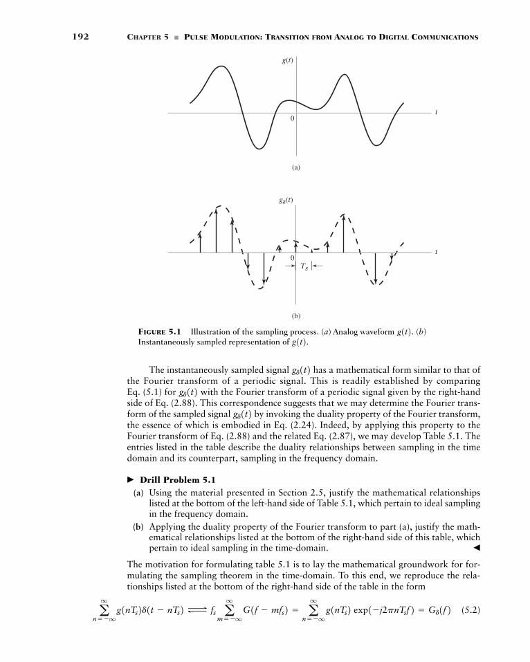
192 CHAPTER 5 � PULSE MODULATION: TRANSITION FROM ANALOG TO DIGITAL COMMUNICATIONS
0
g(t)
t
(b)
(a)
0Ts
g�(t)
t
FIGURE 5.1 Illustration of the sampling process. (a) Analog waveform (b)Instantaneously sampled representation of g1t2. g1t2.
The instantaneously sampled signal has a mathematical form similar to that ofthe Fourier transform of a periodic signal. This is readily established by comparing Eq. (5.1) for with the Fourier transform of a periodic signal given by the right-handside of Eq. (2.88). This correspondence suggests that we may determine the Fourier trans-form of the sampled signal by invoking the duality property of the Fourier transform,the essence of which is embodied in Eq. (2.24). Indeed, by applying this property to theFourier transform of Eq. (2.88) and the related Eq. (2.87), we may develop Table 5.1. Theentries listed in the table describe the duality relationships between sampling in the timedomain and its counterpart, sampling in the frequency domain.
� Drill Problem 5.1(a) Using the material presented in Section 2.5, justify the mathematical relationships
listed at the bottom of the left-hand side of Table 5.1, which pertain to ideal samplingin the frequency domain.
(b) Applying the duality property of the Fourier transform to part (a), justify the math-ematical relationships listed at the bottom of the right-hand side of this table, whichpertain to ideal sampling in the time-domain. �
The motivation for formulating table 5.1 is to lay the mathematical groundwork for for-mulating the sampling theorem in the time-domain. To this end, we reproduce the rela-tionships listed at the bottom of the right-hand side of the table in the form
(5.2)aq
n��qg1nTs2d1t � nTs2 Δ fs a
q
m��qG1f � mfs2 � a
q
n��qg1nTs2 exp1�j2pnTsf2 � Gd1f2
gd1t2gd1t2
gd1t2
5.1 Sampling Process 193
where is the Fourier transform of the original signal and is the sam-pling rate. In words, Eq. (5.2) states that the process of uniformly sampling a continuous-time signal of finite energy results in a periodic spectrum with a repetition frequency equalto the sampling rate.
� SAMPLING THEOREM
The relations of Eq. (5.2) apply to any continuous-time signal of finite energy. Sup-pose, however, that the signal is strictly band-limited, with no frequency componentshigher than W hertz. That is, the Fourier transform of the signal has the prop-erty that is zero for as illustrated in Fig. 5.2(a); the shape of the spectrumshown in this figure is intended for the purpose of illustration only. Suppose also that wechoose the sampling period , which, as we shall see, is the maximum permissi-ble value. Then the corresponding spectrum of the sampled signal is as shownin Fig. 5.2(b). Putting in Eq. (5.2) and using to denote the Fourier trans-form of we may write
(5.3)
Equation (5.3) defines the Fourier transform of the sequence whichis obtained by uniform sampling of a continuous-time signal at the special rate
The formula obtained by using the sampling period shownin Eq. (5.3), is called the discrete-time Fourier transform1 of the sequence 5g1nTs26n���
� .Ts � 1>2W,11>Ts2 � fs � 2W.
g1t25g1n>2W26n���� ,Gd1f2
Gd1f2 � aq
n��qga n
2Wb expa�
jpnf
Wb
gd1t2, Gd1f2Ts � 1>2Wgd1t2Gd1f2Ts � 1>2W
ƒf ƒ � W,G1f2 g1t2G1f2g1t2 g1t2
fs � 1>Tsg1t2,G1f2
1In the Fourier formula of Eq. (5.3), time t is implicitly discretized. If we go one step further and discretize thefrequency too by setting we get the discrete Fourier transform, which is periodic in both time andfrequency; specifically,
where
and
The parameter N is the number of samples in each period, whether in the time or frequency domain. The discreteFourier transform was discussed in Chapter 2.
Gk � Gd12kW2 � Gda kTsb
gn � ga n2Wb � g1nTs2
Gk � aN�1
n�0gn exp1�j2pnk2, k � 0, 1, Á , N � 1
f � k 2W,f
TABLE 5.1 Time-Frequency Sampling-Duality Relationships
Ideal sampling in the frequency domain Ideal sampling in the time domain(Discrete spectrum); see Chapter 2 (Discrete-time function); see this chapter
Fundamental period Sampling rate Delta function Delta function where where Periodicity in the time-domain Periodicity in the frequency domainTime-limited function Band-limited spectrum
aq
n��qg1nTs2e�j2pnTsf � fs a
q
m��qG1f � mfs2a
q
n��qG1nf02d1f � nf02
uuaq
n��qg1nTs2d1t � nTs2T0 a
q
m��qg1t � mT02 � a
q
n��qG1nf02ej2pnf0t
n � 0, �1, �2, Ám � 0, �1, �2, Ád1t � nTs2d1f � mf02,
fs � 1>TsT0 � 1>f0
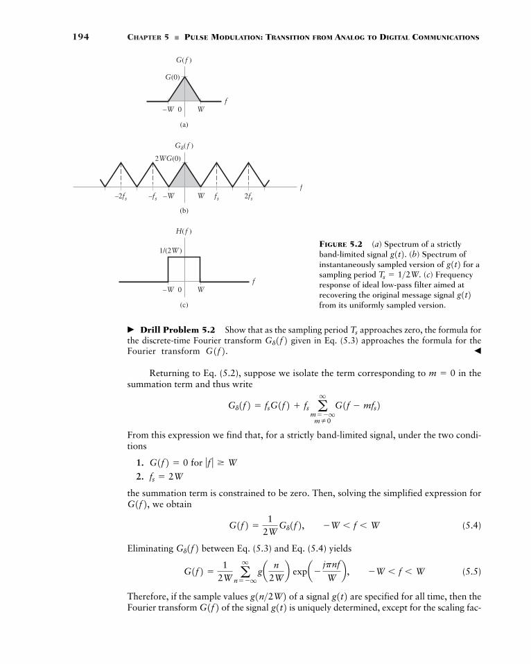
194 CHAPTER 5 � PULSE MODULATION: TRANSITION FROM ANALOG TO DIGITAL COMMUNICATIONS
(a)
(b)
f0–W W
G( f )
G(0)
(c)
f0–W W
H( f )
f–2fs
1/(2W )
2fs–fs fs–W W
G�( f )
2WG(0)
FIGURE 5.2 (a) Spectrum of a strictlyband-limited signal (b) Spectrum ofinstantaneously sampled version of for asampling period (c) Frequencyresponse of ideal low-pass filter aimed atrecovering the original message signal from its uniformly sampled version.
g1t2Ts � 1>2W.
g1t2g1t2.
� Drill Problem 5.2 Show that as the sampling period approaches zero, the formula forthe discrete-time Fourier transform given in Eq. (5.3) approaches the formula for theFourier transform �
Returning to Eq. (5.2), suppose we isolate the term corresponding to in thesummation term and thus write
From this expression we find that, for a strictly band-limited signal, under the two condi-tions
1. for
2.
the summation term is constrained to be zero. Then, solving the simplified expression forwe obtain
(5.4)
Eliminating between Eq. (5.3) and Eq. (5.4) yields
(5.5)
Therefore, if the sample values of a signal are specified for all time, then theFourier transform of the signal is uniquely determined, except for the scaling fac-g1t2G1f2 g1t2g1n>2W2
G1f2 �1
2W aq
n��qga n
2Wb expa�
jpnf
Wb , �W � f � W
Gd1f2G1f2 �
12W
Gd1f2, �W � f � W
G1f2,fs � 2W
ƒf ƒ � WG1f2 � 0
Gd1f2 � fsG1f2 fs aq
m��qm0
G1f � mfs2m � 0
G1f2. Gd1f2 Ts
5.1 Sampling Process 195
tor by the discrete-time Fourier transform of Eq. (5.3) for the spectrum lim-ited to the interval Because is related to by the inverse Fouriertransform, it follows that the signal is itself uniquely determined by the sample values
for In other words, the sequence has all the informa-tion contained in
Consider next the problem of reconstructing the signal from the sequence ofsample values Substituting Eq. (5.5) into the formula for the inverse Fouriertransform defining in terms of we get
We are permitted to interchange the order of summation and integration, as they are bothlinear operations. Accordingly, we may go on to redefine the desired signal as
(5.6)
� Drill Problem 5.3 Show that
�
In light of Problem 5.3, the formula of Eq. (5.6) reduces to
(5.7)
Equation (5.7) is the interpolation formula for reconstructing the original signal fromthe sequence of sample values with the sinc function playing therole of an interpolation function. Each sample is multiplied by a delayed version of theinterpolation function, and all the resulting waveforms are added to obtain
� Drill Problem 5.4 This problem is intended to identify a linear filter for satisfying theinterpolation formula of Eq. (5.7), albeit in a non-physically realizable manner. Equation (5.7)is based on the premise that the signal is strictly limited to the band Withthis specification in mind, consider an ideal low-pass filter whose frequency response isas depicted in Fig. 5.2(c). The impulse response of this filter is defined by (see Eq. (2.25))
Suppose that the correspondingly instantaneously sampled signal defined in Eq. (5.1)is applied to this ideal low-pass filter. With this background, use the convolution integral toshow that the resulting output of the filter is defined exactly by the interpolation formula ofEq. (5.7). �
In light of Problem 5.4, we may now formally say that the synthesis filter or recon-struction filter aimed at recovering the original strictly band-limited signal from itsinstantaneously sampled version in accordance with Eq. (5.7) consists of an ideallow-pass whose frequency response is limited exactly to the same band as the signal g1t2gd1t2 g1t2
gd1t2h1t2 � sinc12Wt2, �� � t � �
H1f2�W � f � W.g1t2
g1t2.sinc12Wt25g1n>2W26, g1t2
g1t2 � aq
n��qga n
2Wb sinc12Wt � n2, �� � t � �
� sinc12Wt � n21
2W LW
�W exp c j2pfa t �
n2Wb d df �
sin12pWt � np212pWt � np2
g1t2 � aq
n��qga n
2Wb 1
2WLW
�W expc j2pf at �
n2Wb d df
g1t2
� LW
�W
12W a
q
n��qga n
2Wb expa�
jpnf
Wb exp1j2pft2 df
g1t2 � Lq
�qG1f2 exp1j2pft2 df
G1f2,g1t25g1n>2W26. g1t2g1t2. 5g1n>2W26�� � n � �.g1n>2W2 g1t2 G1f2g1t2�W � f � W.Gd1f21>2W,
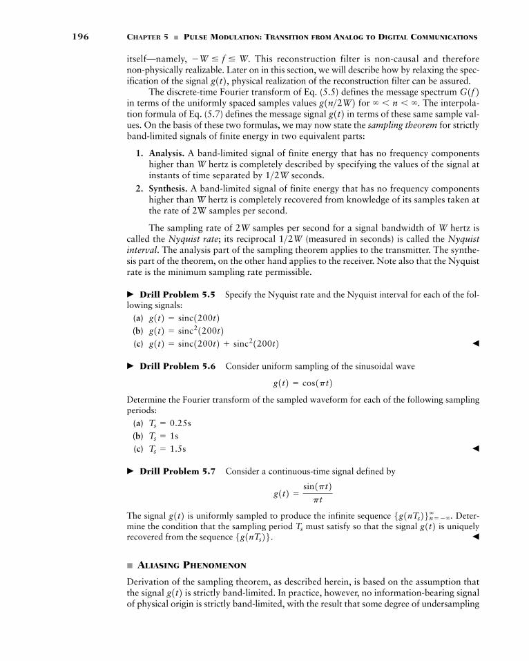
196 CHAPTER 5 � PULSE MODULATION: TRANSITION FROM ANALOG TO DIGITAL COMMUNICATIONS
itself—namely, This reconstruction filter is non-causal and therefore non-physically realizable. Later on in this section, we will describe how by relaxing the spec-ification of the signal physical realization of the reconstruction filter can be assured.
The discrete-time Fourier transform of Eq. (5.5) defines the message spectrum in terms of the uniformly spaced samples values for The interpola-tion formula of Eq. (5.7) defines the message signal in terms of these same sample val-ues. On the basis of these two formulas, we may now state the sampling theorem for strictlyband-limited signals of finite energy in two equivalent parts:
1. Analysis. A band-limited signal of finite energy that has no frequency componentshigher than W hertz is completely described by specifying the values of the signal atinstants of time separated by seconds.
2. Synthesis. A band-limited signal of finite energy that has no frequency componentshigher than W hertz is completely recovered from knowledge of its samples taken atthe rate of 2W samples per second.
The sampling rate of 2W samples per second for a signal bandwidth of W hertz iscalled the Nyquist rate; its reciprocal (measured in seconds) is called the Nyquistinterval. The analysis part of the sampling theorem applies to the transmitter. The synthe-sis part of the theorem, on the other hand applies to the receiver. Note also that the Nyquistrate is the minimum sampling rate permissible.
� Drill Problem 5.5 Specify the Nyquist rate and the Nyquist interval for each of the fol-lowing signals:
(a)(b)(c) �
� Drill Problem 5.6 Consider uniform sampling of the sinusoidal wave
Determine the Fourier transform of the sampled waveform for each of the following samplingperiods:
(a)(b)(c) �
� Drill Problem 5.7 Consider a continuous-time signal defined by
The signal is uniformly sampled to produce the infinite sequence Deter-mine the condition that the sampling period must satisfy so that the signal is uniquelyrecovered from the sequence �
� ALIASING PHENOMENON
Derivation of the sampling theorem, as described herein, is based on the assumption thatthe signal is strictly band-limited. In practice, however, no information-bearing signalof physical origin is strictly band-limited, with the result that some degree of undersampling
g1t2
5g1nTs26. g1t2Ts
5g1nTs26n� ��� .g1t2
g1t2 �sin1pt2pt
Ts � 1.5s
Ts � 1s
Ts � 0.25s
g1t2 � cos1pt2
g1t2 � sinc1200t2 sinc21200t2g1t2 � sinc21200t2g1t2 � sinc1200t2
1>2W
1>2W
g1t2 � � n � �.g1n>2W2 G1f2g1t2,�W � f � W.
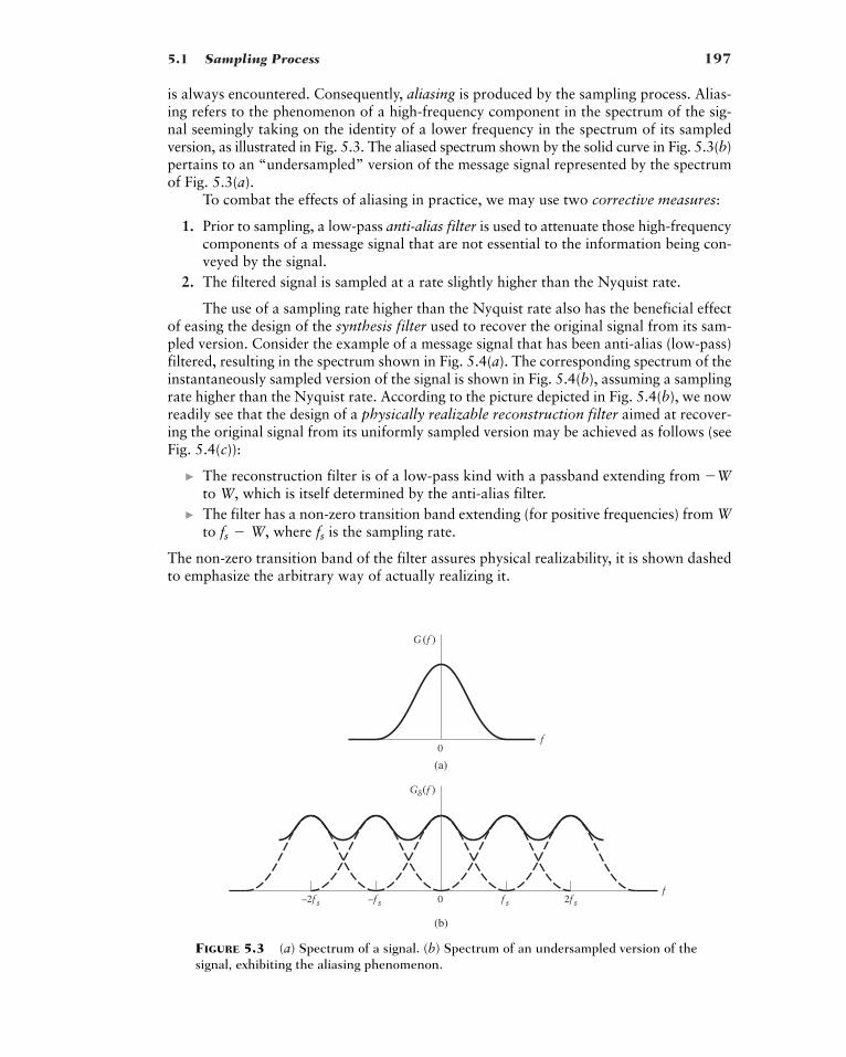
5.1 Sampling Process 197
G(f )
f
0
0
f
G�(f )
2f sf s–f s–2f s
(a)
(b)
FIGURE 5.3 (a) Spectrum of a signal. (b) Spectrum of an undersampled version of thesignal, exhibiting the aliasing phenomenon.
is always encountered. Consequently, aliasing is produced by the sampling process. Alias-ing refers to the phenomenon of a high-frequency component in the spectrum of the sig-nal seemingly taking on the identity of a lower frequency in the spectrum of its sampledversion, as illustrated in Fig. 5.3. The aliased spectrum shown by the solid curve in Fig. 5.3(b)pertains to an “undersampled” version of the message signal represented by the spectrumof Fig. 5.3(a).
To combat the effects of aliasing in practice, we may use two corrective measures:
1. Prior to sampling, a low-pass anti-alias filter is used to attenuate those high-frequencycomponents of a message signal that are not essential to the information being con-veyed by the signal.
2. The filtered signal is sampled at a rate slightly higher than the Nyquist rate.
The use of a sampling rate higher than the Nyquist rate also has the beneficial effectof easing the design of the synthesis filter used to recover the original signal from its sam-pled version. Consider the example of a message signal that has been anti-alias (low-pass)filtered, resulting in the spectrum shown in Fig. 5.4(a). The corresponding spectrum of theinstantaneously sampled version of the signal is shown in Fig. 5.4(b), assuming a samplingrate higher than the Nyquist rate. According to the picture depicted in Fig. 5.4(b), we nowreadily see that the design of a physically realizable reconstruction filter aimed at recover-ing the original signal from its uniformly sampled version may be achieved as follows (seeFig. 5.4(c)):
� The reconstruction filter is of a low-pass kind with a passband extending from to W, which is itself determined by the anti-alias filter.
� The filter has a non-zero transition band extending (for positive frequencies) from Wto where is the sampling rate.
The non-zero transition band of the filter assures physical realizability, it is shown dashedto emphasize the arbitrary way of actually realizing it.
fsfs � W,
�W
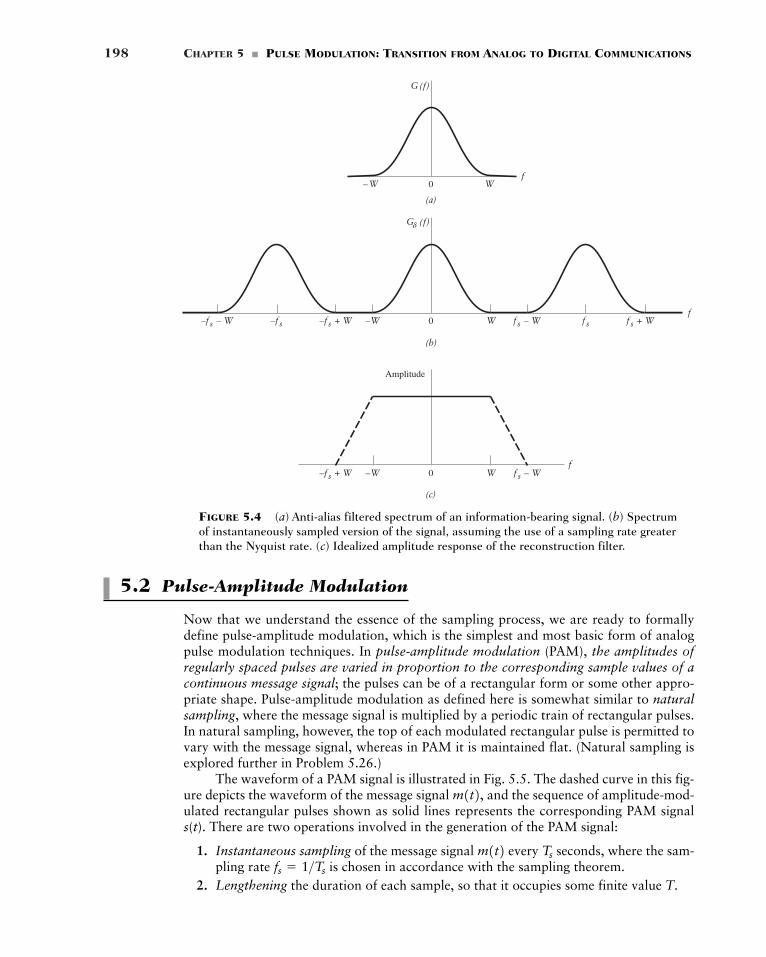
198 CHAPTER 5 � PULSE MODULATION: TRANSITION FROM ANALOG TO DIGITAL COMMUNICATIONS
G(f)
f
0
0
f
G (f)�
–f s
(a)
(b)
f
(c)
–W W
–fs – W –fs + W –W W fs + Wfs – W fs
0–f s + W –W W fs – W
Amplitude
FIGURE 5.4 (a) Anti-alias filtered spectrum of an information-bearing signal. (b) Spectrumof instantaneously sampled version of the signal, assuming the use of a sampling rate greaterthan the Nyquist rate. (c) Idealized amplitude response of the reconstruction filter.
5.2 Pulse-Amplitude Modulation
Now that we understand the essence of the sampling process, we are ready to formallydefine pulse-amplitude modulation, which is the simplest and most basic form of analogpulse modulation techniques. In pulse-amplitude modulation (PAM), the amplitudes ofregularly spaced pulses are varied in proportion to the corresponding sample values of acontinuous message signal; the pulses can be of a rectangular form or some other appro-priate shape. Pulse-amplitude modulation as defined here is somewhat similar to naturalsampling, where the message signal is multiplied by a periodic train of rectangular pulses.In natural sampling, however, the top of each modulated rectangular pulse is permitted tovary with the message signal, whereas in PAM it is maintained flat. (Natural sampling isexplored further in Problem 5.26.)
The waveform of a PAM signal is illustrated in Fig. 5.5. The dashed curve in this fig-ure depicts the waveform of the message signal and the sequence of amplitude-mod-ulated rectangular pulses shown as solid lines represents the corresponding PAM signals(t). There are two operations involved in the generation of the PAM signal:
1. Instantaneous sampling of the message signal every seconds, where the sam-pling rate is chosen in accordance with the sampling theorem.
2. Lengthening the duration of each sample, so that it occupies some finite value T.fs � 1>Ts
Tsm1t2
m1t2,
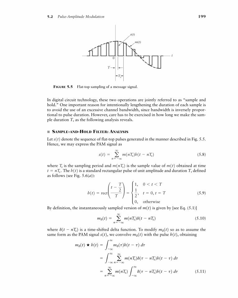
5.2 Pulse-Amplitude Modulation 199
Ts
s(t)
t
m(t)
T
0
FIGURE 5.5 Flat-top sampling of a message signal.
In digital circuit technology, these two operations are jointly referred to as “sample andhold.” One important reason for intentionally lengthening the duration of each sample isto avoid the use of an excessive channel bandwidth, since bandwidth is inversely propor-tional to pulse duration. However, care has to be exercised in how long we make the sam-ple duration T, as the following analysis reveals.
� SAMPLE-AND-HOLD FILTER: ANALYSIS
Let denote the sequence of flat-top pulses generated in the manner described in Fig. 5.5.Hence, we may express the PAM signal as
(5.8)
where is the sampling period and is the sample value of obtained at timeThe is a standard rectangular pulse of unit amplitude and duration T, defined
as follows (see Fig. 5.6(a)):
(5.9)
By definition, the instantaneously sampled version of is given by [see Eq. (5.1)]
(5.10)
where is a time-shifted delta function. To modify so as to assume thesame form as the PAM signal we convolve with the pulse obtaining
(5.11)� aq
n��qm1nTs2L
q
�qd1t � nTs2h1t � t2 dt
� Lq
�qaq
n��qm1nTs2d1t � nTs2h1t � t2 dt
md1t2 � h1t2 � Lq
�qmd1t2h1t � t2 dt
h1t2,md1t2s1t2, md1t2d1t � nTs2md1t2 � a
q
n��qm1nTs2d1t � nTs2
m1t2h1t2 � rect
£ t �T2
T≥
� d 1, 0 � t � T12
, t � 0, t � T
0, otherwise
h1t2t � nTs .m1t2m1nTs2Ts
s1t2 � aq
n��qm1nTs2h1t � nTs2
s1t2
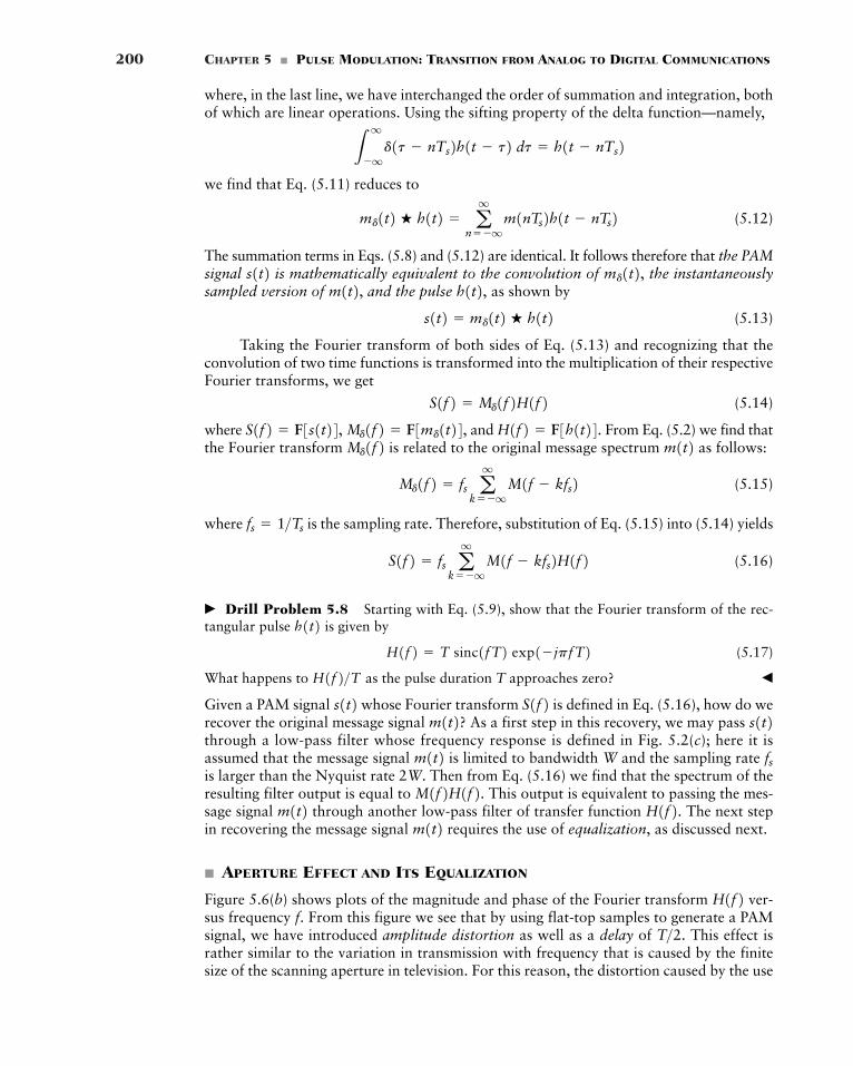
200 CHAPTER 5 � PULSE MODULATION: TRANSITION FROM ANALOG TO DIGITAL COMMUNICATIONS
where, in the last line, we have interchanged the order of summation and integration, bothof which are linear operations. Using the sifting property of the delta function—namely,
we find that Eq. (5.11) reduces to
(5.12)
The summation terms in Eqs. (5.8) and (5.12) are identical. It follows therefore that the PAMsignal is mathematically equivalent to the convolution of the instantaneouslysampled version of and the pulse as shown by
(5.13)
Taking the Fourier transform of both sides of Eq. (5.13) and recognizing that theconvolution of two time functions is transformed into the multiplication of their respectiveFourier transforms, we get
(5.14)
where and From Eq. (5.2) we find thatthe Fourier transform is related to the original message spectrum as follows:
(5.15)
where is the sampling rate. Therefore, substitution of Eq. (5.15) into (5.14) yields
(5.16)
� Drill Problem 5.8 Starting with Eq. (5.9), show that the Fourier transform of the rec-tangular pulse is given by
(5.17)
What happens to as the pulse duration T approaches zero? �
Given a PAM signal whose Fourier transform is defined in Eq. (5.16), how do werecover the original message signal As a first step in this recovery, we may pass through a low-pass filter whose frequency response is defined in Fig. 5.2(c); here it isassumed that the message signal is limited to bandwidth W and the sampling rate is larger than the Nyquist rate 2W. Then from Eq. (5.16) we find that the spectrum of theresulting filter output is equal to This output is equivalent to passing the mes-sage signal through another low-pass filter of transfer function The next stepin recovering the message signal requires the use of equalization, as discussed next.
� APERTURE EFFECT AND ITS EQUALIZATION
Figure 5.6(b) shows plots of the magnitude and phase of the Fourier transform ver-sus frequency From this figure we see that by using flat-top samples to generate a PAMsignal, we have introduced amplitude distortion as well as a delay of This effect israther similar to the variation in transmission with frequency that is caused by the finitesize of the scanning aperture in television. For this reason, the distortion caused by the use
T>2.f.
H1f2
m1t2 H1f2.m1t2 M1f2H1f2.fsm1t2
s1t2m1t2? S1f2s1t2H1f2>T
H1f2 � T sinc1fT2 exp1�jpfT2h1t2
S1f2 � fs aq
k��qM1f � kfs2H1f2
fs � 1>Ts
Md1f2 � fs aq
k��qM1f � kfs2
m1t2Md1f2 H1f2 � F3h1t24.S1f2 � F3s1t24, Md1f2 � F3md1t24,S1f2 � Md1f2H1f2
s1t2 � md1t2 � h1t2h1t2,m1t2, md1t2,s1t2
md1t2 � h1t2 � aq
n��qm1nTs2h1t � nTs2
Lq
�qd1t � nTs2h1t � t2 dt � h1t � nTs2
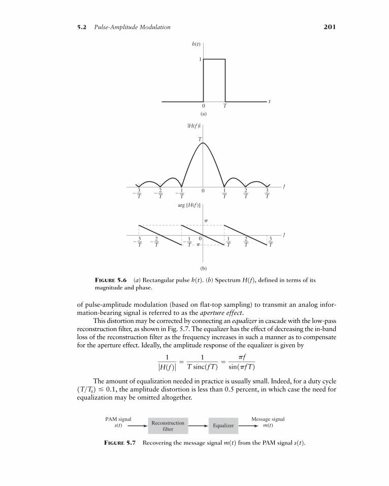
5.2 Pulse-Amplitude Modulation 201
of pulse-amplitude modulation (based on flat-top sampling) to transmit an analog infor-mation-bearing signal is referred to as the aperture effect.
This distortion may be corrected by connecting an equalizer in cascade with the low-passreconstruction filter, as shown in Fig. 5.7. The equalizer has the effect of decreasing the in-bandloss of the reconstruction filter as the frequency increases in such a manner as to compensatefor the aperture effect. Ideally, the amplitude response of the equalizer is given by
The amount of equalization needed in practice is usually small. Indeed, for a duty cyclethe amplitude distortion is less than 0.5 percent, in which case the need for
equalization may be omitted altogether.1T>Ts2 � 0.1,
1
ƒH1f2 ƒ �1
T sinc1fT2 �pf
sin1pfT2
h(t)
tT0
(a)
(b)
1
|H(f )|
f0
T
—–– 3T
—–– 2T
—–– 1T
—–1T
—–2T
—–3T
arg [H(f )]
f0
�
�
—–– 3T
—–– 2T
—–– 1T
—–1T
—–2T
—–3T
FIGURE 5.6 (a) Rectangular pulse (b) Spectrum defined in terms of itsmagnitude and phase.
H1f2,h1t2.
PAM signals(t)
Message signalm(t)Reconstruction
filterEqualizer
FIGURE 5.7 Recovering the message signal from the PAM signal s1t2.m1t2
202 CHAPTER 5 � PULSE MODULATION: TRANSITION FROM ANALOG TO DIGITAL COMMUNICATIONS
The transmission of a PAM signal imposes rather stringent requirements on the ampli-tude and phase responses of the channel, because of the relatively short duration of the trans-mitted pulses. Furthermore, it may be shown that the noise performance of a PAM systemcan never be better than direct transmission of the message signal. Accordingly, we find thatfor transmission over long distances, PAM would be used only as a means of message pro-cessing for time-division multiplexing. The concept of time-division multiplexing is dis-cussed later in this chapter.
5.3 Pulse-Position Modulation
In pulse-amplitude modulation, pulse amplitude is the variable parameter. Pulse durationis the next logical parameter available for modulation. In pulse-duration modulation (PDM),the samples of the message signal are used to vary the duration of the individual pulses. Thisform of modulation is also referred to as pulse-width modulation or pulse-length modula-tion. The modulating signal may vary the time of occurrence of the leading edge, the trail-ing edge, or both edges of the pulse. In Fig. 5.8(c) the trailing edge of each pulse is variedin accordance with the message signal, assumed to be sinusoidal as shown in Fig. 5.8(a).The periodic pulse carrier is shown in Fig. 5.8(b).
m(t)
(a)
(b)
(c)
(d) Time
FIGURE 5.8 Illustration of two different forms of pulse-time modulation for the case of asinusoidal modulating wave. (a) Modulating wave. (b) Pulse carrier. (c) PDM wave. (d) PPMwave.
5.4 Completing the Transition from Analog to Digital 203
PDM is wasteful of power, in that long pulses expend considerable power during thepulse while bearing no additional information. If this unused power is subtracted fromPDM, so that only time transitions are essentially preserved, we obtain a more efficienttype of pulse modulation known as pulse-position modulation (PPM). In PPM, the posi-tion of a pulse relative to its unmodulated time of occurrence is varied in accordance withthe message signal, as illustrated in Fig. 5.8(d) for the case of sinusoidal modulation.
Let denote the sample duration. Using the sample of a message signal to modulate the position of the nth pulse, we obtain the PPM signal
(5.18)
where is the sensitivity factor of the pulse-position modulator (in seconds per volt) anddenotes a standard pulse of interest. Clearly, the different pulses constituting the PPM
signal must be strictly nonoverlapping; a sufficient condition for this requirement to besatisfied is to have
(5.19)
which, in turn, requires that(5.20)
The closer is to one half the sampling duration the narrower must the stan-dard pulse be to ensure that the individual pulses of the PPM signal do not inter-fere with each other, and the wider will the bandwidth occupied by the PPM signal be.Assuming that Eq. (5.19) is satisfied and that there is no interference between adjacentpulses of the PPM signal then the signal samples can be recovered perfectly.2
Furthermore, if the message signal is strictly band-limited, it follows from the sam-pling theorem that the original message signal can be recovered from the PPM signal
without distortion.
5.4 Completing the Transition from Analog to Digital
At this point in the book, it is instructive that we look at the modulation techniques thatwe have studied thus far, for transmitting analog information-bearing signals (i.e., voice andvideo signals) over a communication channel, and look at those that are yet to be consid-ered. The techniques studied thus far are continuous-wave modulation and analog pulsemodulation. Although, these two families of modulation techniques are indeed different,they share similar attributes and limitations.
First, it is natural to think of pulse-amplitude modulation as the counterpart of ampli-tude modulation studied in Chapter 3. What do we have as a pulse-modulation counter-part to frequency modulation studied in Chapter 4? In frequency modulation, thezero-crossings of the modulated wave vary with time in accordance with the message sig-nal. In pulse-position modulation, the positions of transmitted pulses vary with time inaccordance with the message signal. In a loose sense, we may therefore think of pulse-posi-tion modulation as the counterpart of frequency modulation.
An intuitive conclusion to draw from this loose analogy between members of analogpulse modulation and those of continuous-wave modulation is that these two families ofmodulation techniques offer the same order of performance when they are applied to thetransmission of analog signals over communication channels. In the context of performance,we are thinking in terms of transmission bandwidth requirement and receiver noise behavior.
s1t2 m1t2m1t2 m1nTs2s1t2,s1t2g1t2 Ts ,kp ƒm1t2 ƒmax
kp ƒm1t2 ƒmax � 1Ts>22g1t2 � 0, ƒt ƒ � 1Ts>22 � kp ƒm1t2 ƒmax
s1t2g1t2 kp
s1t2 � aq
n��qg1t � nTs � kpm1nTs22
m1t2m1nTs2Ts
2Generation and detection of PPM waves are discussed in Haykin (1994), pp. 365–369.
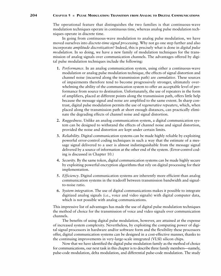
204 CHAPTER 5 � PULSE MODULATION: TRANSITION FROM ANALOG TO DIGITAL COMMUNICATIONS
The operational feature that distinguishes the two families is that continuous-wavemodulation techniques operate in continuous time, whereas analog pulse modulation tech-niques operate in discrete time.
In going from continuous-wave modulation to analog pulse modulation, we havemoved ourselves into discrete-time signal processing. Why not go one step further and alsoincorporate amplitude discretization? Indeed, this is precisely what is done in digital pulsemodulation. In so doing, we have a new family of modulation techniques for the trans-mission of analog signals over communication channels. The advantages offered by digi-tal pulse modulation techniques include the following:
1. Performance. In an analog communication system, using either a continuous-wavemodulation or analog pulse modulation technique, the effects of signal distortion andchannel noise (incurred along the transmission path) are cumulative. These sourcesof impairments therefore tend to become progressively stronger, ultimately over-whelming the ability of the communication system to offer an acceptable level of per-formance from source to destination. Unfortunately, the use of repeaters in the formof amplifiers, placed at different points along the transmission path, offers little helpbecause the message signal and noise are amplified to the same extent. In sharp con-trast, digital pulse modulation permits the use of regenerative repeaters, which, whenplaced along the transmission path at short enough distances, can practically elimi-nate the degrading effects of channel noise and signal distortion.
2. Ruggedness. Unlike an analog communication system, a digital communication sys-tem can be designed to withstand the effects of channel noise and signal distortion,provided the noise and distortion are kept under certain limits.
3. Reliability. Digital communication systems can be made highly reliable by exploitingpowerful error-control coding techniques in such a way that the estimate of a mes-sage signal delivered to a user is almost indistinguishable from the message signaldelivered by a source of information at the other end of the system. (Error-control cod-ing is discussed in Chapter 10.)
4. Security. By the same token, digital communication systems can be made highly secureby exploiting powerful encryption algorithms that rely on digital processing for theirimplementation.
5. Efficiency. Digital communication systems are inherently more efficient than analogcommunication systems in the tradeoff between transmission bandwidth and signal-to-noise ratio.
6. System integration. The use of digital communications makes it possible to integratedigitized analog signals (i.e., voice and video signals) with digital computer data,which is not possible with analog communications.
This impressive list of advantages has made the use of digital pulse modulation techniquesthe method of choice for the transmission of voice and video signals over communicationchannels.
The benefits of using digital pulse modulation, however, are attained at the expenseof increased system complexity. Nevertheless, by exploiting the computing power of digi-tal signal processors in hardware and/or software form and the flexibility these processorsoffer, digital communication systems can be designed in a cost-effective manner, thanks tothe continuing improvements in very-large-scale integrated (VLSI) silicon chips.
Now that we have identified the digital pulse modulation family as the method of choicefor communications, our next task in this chapter is to describe three family members—namely,pulse-code modulation, delta modulation, and differential pulse-code modulation. The study
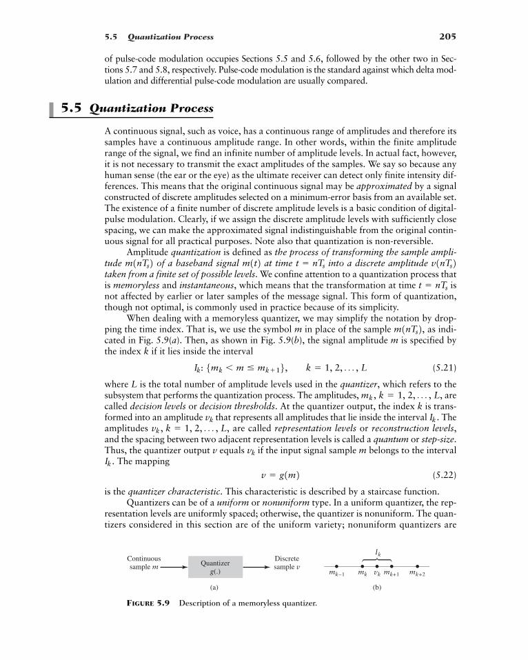
5.5 Quantization Process 205
of pulse-code modulation occupies Sections 5.5 and 5.6, followed by the other two in Sec-tions 5.7 and 5.8, respectively. Pulse-code modulation is the standard against which delta mod-ulation and differential pulse-code modulation are usually compared.
5.5 Quantization Process
A continuous signal, such as voice, has a continuous range of amplitudes and therefore itssamples have a continuous amplitude range. In other words, within the finite amplituderange of the signal, we find an infinite number of amplitude levels. In actual fact, however,it is not necessary to transmit the exact amplitudes of the samples. We say so because anyhuman sense (the ear or the eye) as the ultimate receiver can detect only finite intensity dif-ferences. This means that the original continuous signal may be approximated by a signalconstructed of discrete amplitudes selected on a minimum-error basis from an available set.The existence of a finite number of discrete amplitude levels is a basic condition of digital-pulse modulation. Clearly, if we assign the discrete amplitude levels with sufficiently closespacing, we can make the approximated signal indistinguishable from the original contin-uous signal for all practical purposes. Note also that quantization is non-reversible.
Amplitude quantization is defined as the process of transforming the sample ampli-tude of a baseband signal at time into a discrete amplitudetaken from a finite set of possible levels. We confine attention to a quantization process thatis memoryless and instantaneous, which means that the transformation at time isnot affected by earlier or later samples of the message signal. This form of quantization,though not optimal, is commonly used in practice because of its simplicity.
When dealing with a memoryless quantizer, we may simplify the notation by drop-ping the time index. That is, we use the symbol m in place of the sample as indi-cated in Fig. 5.9(a). Then, as shown in Fig. 5.9(b), the signal amplitude m is specified bythe index k if it lies inside the interval
(5.21)
where L is the total number of amplitude levels used in the quantizer, which refers to thesubsystem that performs the quantization process. The amplitudes, arecalled decision levels or decision thresholds. At the quantizer output, the index k is trans-formed into an amplitude that represents all amplitudes that lie inside the interval Theamplitudes are called representation levels or reconstruction levels,and the spacing between two adjacent representation levels is called a quantum or step-size.Thus, the quantizer output equals if the input signal sample m belongs to the interval
The mapping
(5.22)
is the quantizer characteristic. This characteristic is described by a staircase function.Quantizers can be of a uniform or nonuniform type. In a uniform quantizer, the rep-
resentation levels are uniformly spaced; otherwise, the quantizer is nonuniform. The quan-tizers considered in this section are of the uniform variety; nonuniform quantizers are
v � g1m2Ik .
vkv
vk , k � 1, 2, Á , L,Ik .vk
mk , k � 1, 2, Á , L,
Ik: 5mk � m � mk16, k � 1, 2, Á , L
m1nTs2,
t � nTs
v1nTs2t � nTsm1t2m1nTs2
(a) (b)
Continuoussample m
Discretesample vQuantizer
g(.) mk–1 mk
Ik
vk mk+2mk+1
FIGURE 5.9 Description of a memoryless quantizer.
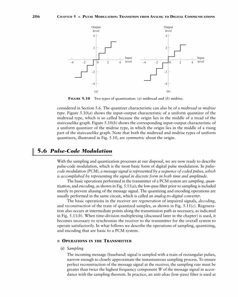
206 CHAPTER 5 � PULSE MODULATION: TRANSITION FROM ANALOG TO DIGITAL COMMUNICATIONS
considered in Section 5.6. The quantizer characteristic can also be of a midtread or midrisetype. Figure 5.10(a) shows the input–output characteristic of a uniform quantizer of themidtread type, which is so called because the origin lies in the middle of a tread of thestaircaselike graph. Figure 5.10(b) shows the corresponding input–output characteristic ofa uniform quantizer of the midrise type, in which the origin lies in the middle of a risingpart of the staircaselike graph. Note that both the midtread and midrise types of uniformquantizers, illustrated in Fig. 5.10, are symmetric about the origin.
5.6 Pulse-Code Modulation
With the sampling and quantization processes at our disposal, we are now ready to describepulse-code modulation, which is the most basic form of digital pulse modulation. In pulse-code modulation (PCM), a message signal is represented by a sequence of coded pulses, whichis accomplished by representing the signal in discrete form in both time and amplitude.
The basic operations performed in the transmitter of a PCM system are sampling, quan-tization, and encoding, as shown in Fig. 5.11(a); the low-pass filter prior to sampling is includedmerely to prevent aliasing of the message signal. The quantizing and encoding operations areusually performed in the same circuit, which is called an analog-to-digital converter.
The basic operations in the receiver are regeneration of impaired signals, decoding,and reconstruction of the train of quantized samples, as shown in Fig. 5.11(c). Regenera-tion also occurs at intermediate points along the transmission path as necessary, as indicatedin Fig. 5.11(b). When time-division multiplexing (discussed later in the chapter) is used, itbecomes necessary to synchronize the receiver to the transmitter for the overall system tooperate satisfactorily. In what follows we describe the operations of sampling, quantizing,and encoding that are basic to a PCM system.
� OPERATIONS IN THE TRANSMITTER
(i) Sampling
The incoming message (baseband) signal is sampled with a train of rectangular pulses,narrow enough to closely approximate the instantaneous sampling process. To ensureperfect reconstruction of the message signal at the receiver, the sampling rate must begreater than twice the highest frequency component W of the message signal in accor-dance with the sampling theorem. In practice, an anti-alias (low-pass) filter is used at
420–2–4
4
2
–2
–4
Outputlevel
(a)
Inputlevel 420–2–4
4
2
–2
–4
Outputlevel
(b)
Inputlevel
FIGURE 5.10 Two types of quantization: (a) midtread and (b) midrise.
5.6 Pulse-Code Modulation 207
(a)
Source ofcontinuous-
time messagesignal
Low-passfilter
Sampler Quantizer EncoderPCMdata
sequence
(b)
Transmissionline
Transmissionline
Regenerativerepeater
Transmissionline
Channeloutput
Regenerativerepeater
PCMdata
shapedfor
transmission
...
Regenerativecircuit
Reconstructionfilter
DestinationDecoderChanneloutput
(c)
FIGURE 5.11 The basic elements of a PCM system: (a) Transmitter, (b) transmission path,connecting the transmitter to the receiver, and (c) receiver.
the front end of the sampler in order to exclude frequencies greater than W before sam-pling, as shown in Fig. 5.11(a). Thus the application of sampling permits the reduc-tion of the continuously varying message signal (of some finite duration) to a limitednumber of discrete values per second.
(ii) Nonuniform QuantizationThe sampled version of the message signal is then quantized, thereby providing a newrepresentation of the signal that is discrete in both time and amplitude. The quanti-zation process may follow a uniform law as described in Section 5.5. In certain appli-cations, however, it is preferable to use a variable separation between therepresentation levels. For example, the range of voltages covered by voice signals,from the peaks of loud talk to the weak passages of weak talk, is on the order of1000 to 1. By using a nonuniform quantizer with the feature that the step size increasesas the separation from the origin of the input–output amplitude characteristic isincreased, the large end-step of the quantizer can take care of possible excursions ofthe voice signal into the large amplitude ranges that occur relatively infrequently. Inother words, the weak passages that need more protection are favored at the expenseof the loud passages. In this way, a nearly uniform percentage precision is achievedthroughout the greater part of the amplitude range of the input signal, with the resultthat fewer steps are needed than would be the case if a uniform quantizer were used.
The use of a nonuniform quantizer is equivalent to passing the message signalthrough a compressor and then applying the compressed signal to a uniform quan-tizer. A particular form of compression law that is used in practice is the so called
3 defined by
(5.23)ƒv ƒ �log11 m ƒm ƒ2
log11 m2m-law
3The used for signal compression is described in Smith (1957); this compression law is used in the United States,Canada, and Japan. In Europe, the A-law is used for signal compression; this second compression law is described inCattermole (1969, pp. 133–140). For discussion of the and A-law, see also the paper by Kaneko (1970).m-law
m-law
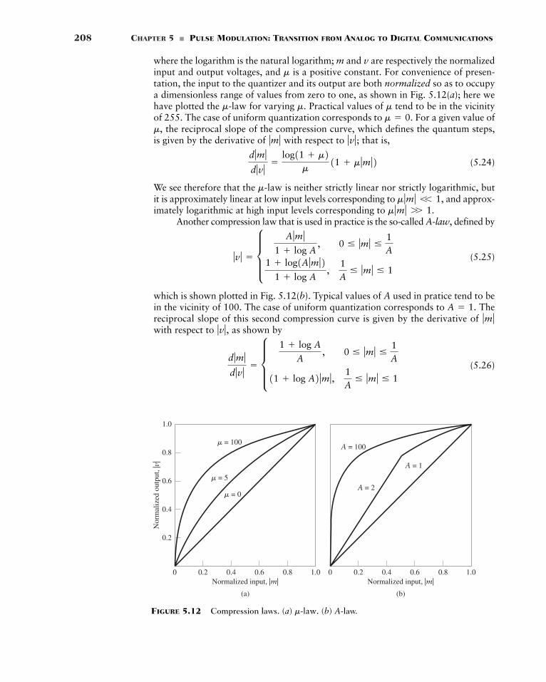
208 CHAPTER 5 � PULSE MODULATION: TRANSITION FROM ANALOG TO DIGITAL COMMUNICATIONS
where the logarithm is the natural logarithm; m and are respectively the normalizedinput and output voltages, and is a positive constant. For convenience of presen-tation, the input to the quantizer and its output are both normalized so as to occupya dimensionless range of values from zero to one, as shown in Fig. 5.12(a); here wehave plotted the for varying Practical values of tend to be in the vicinityof 255. The case of uniform quantization corresponds to For a given value of
the reciprocal slope of the compression curve, which defines the quantum steps,is given by the derivative of with respect to that is,
(5.24)
We see therefore that the is neither strictly linear nor strictly logarithmic, butit is approximately linear at low input levels corresponding to and approx-imately logarithmic at high input levels corresponding to
Another compression law that is used in practice is the so-called A-law, defined by
(5.25)
which is shown plotted in Fig. 5.12(b). Typical values of A used in pratice tend to bein the vicinity of 100. The case of uniform quantization corresponds to Thereciprocal slope of this second compression curve is given by the derivative of with respect to as shown by
(5.26)d ƒm ƒd ƒv ƒ
� d 1 log A
A, 0 � ƒm ƒ �
1A
11 log A2 ƒm ƒ ,1A
� ƒm ƒ � 1
ƒv ƒ ,ƒm ƒ
A � 1.
ƒv ƒ � d A ƒm ƒ1 log A
, 0 � ƒm ƒ �1A
1 log1A ƒm ƒ21 log A
,1A
� ƒm ƒ � 1
m ƒm ƒ W 1.m ƒm ƒ V 1,
m-law
d ƒm ƒd ƒv ƒ
�log11 m2
m11 m ƒm ƒ2
ƒv ƒ ;ƒm ƒm,
m � 0.mm.m-law
m
v
(a)
0 0.2 0.4 0.6 0.8Normalized input, |m|
1.0
� = 100
� = 5
� = 0
0.2
0.4
Nor
mal
ized
out
put,
|v|
0.6
0.8
1.0
(b)
0 0.2 0.4 0.6 0.8Normalized input, |m|
1.0
A = 100
A = 2
A = 1
FIGURE 5.12 Compression laws. (a) (b) A-law.m-law.
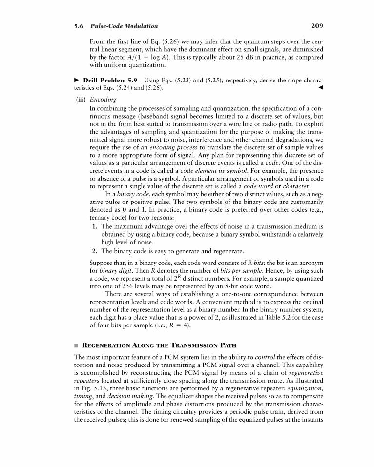
5.6 Pulse-Code Modulation 209
From the first line of Eq. (5.26) we may infer that the quantum steps over the cen-tral linear segment, which have the dominant effect on small signals, are diminishedby the factor This is typically about 25 dB in practice, as comparedwith uniform quantization.
� Drill Problem 5.9 Using Eqs. (5.23) and (5.25), respectively, derive the slope charac-teristics of Eqs. (5.24) and (5.26). �
(iii) EncodingIn combining the processes of sampling and quantization, the specification of a con-tinuous message (baseband) signal becomes limited to a discrete set of values, butnot in the form best suited to transmission over a wire line or radio path. To exploitthe advantages of sampling and quantization for the purpose of making the trans-mitted signal more robust to noise, interference and other channel degradations, werequire the use of an encoding process to translate the discrete set of sample valuesto a more appropriate form of signal. Any plan for representing this discrete set ofvalues as a particular arrangement of discrete events is called a code. One of the dis-crete events in a code is called a code element or symbol. For example, the presenceor absence of a pulse is a symbol. A particular arrangement of symbols used in a codeto represent a single value of the discrete set is called a code word or character.
In a binary code, each symbol may be either of two distinct values, such as a neg-ative pulse or positive pulse. The two symbols of the binary code are customarilydenoted as 0 and 1. In practice, a binary code is preferred over other codes (e.g.,ternary code) for two reasons:1. The maximum advantage over the effects of noise in a transmission medium is
obtained by using a binary code, because a binary symbol withstands a relativelyhigh level of noise.
2. The binary code is easy to generate and regenerate.
Suppose that, in a binary code, each code word consists of R bits: the bit is an acronymfor binary digit. Then R denotes the number of bits per sample. Hence, by using sucha code, we represent a total of distinct numbers. For example, a sample quantizedinto one of 256 levels may be represented by an 8-bit code word.
There are several ways of establishing a one-to-one correspondence betweenrepresentation levels and code words. A convenient method is to express the ordinalnumber of the representation level as a binary number. In the binary number system,each digit has a place-value that is a power of 2, as illustrated in Table 5.2 for the caseof four bits per sample (i.e., ).
� REGENERATION ALONG THE TRANSMISSION PATH
The most important feature of a PCM system lies in the ability to control the effects of dis-tortion and noise produced by transmitting a PCM signal over a channel. This capabilityis accomplished by reconstructing the PCM signal by means of a chain of regenerativerepeaters located at sufficiently close spacing along the transmission route. As illustratedin Fig. 5.13, three basic functions are performed by a regenerative repeater: equalization,timing, and decision making. The equalizer shapes the received pulses so as to compensatefor the effects of amplitude and phase distortions produced by the transmission charac-teristics of the channel. The timing circuitry provides a periodic pulse train, derived fromthe received pulses; this is done for renewed sampling of the equalized pulses at the instants
R � 4
2R
A>11 log A2.
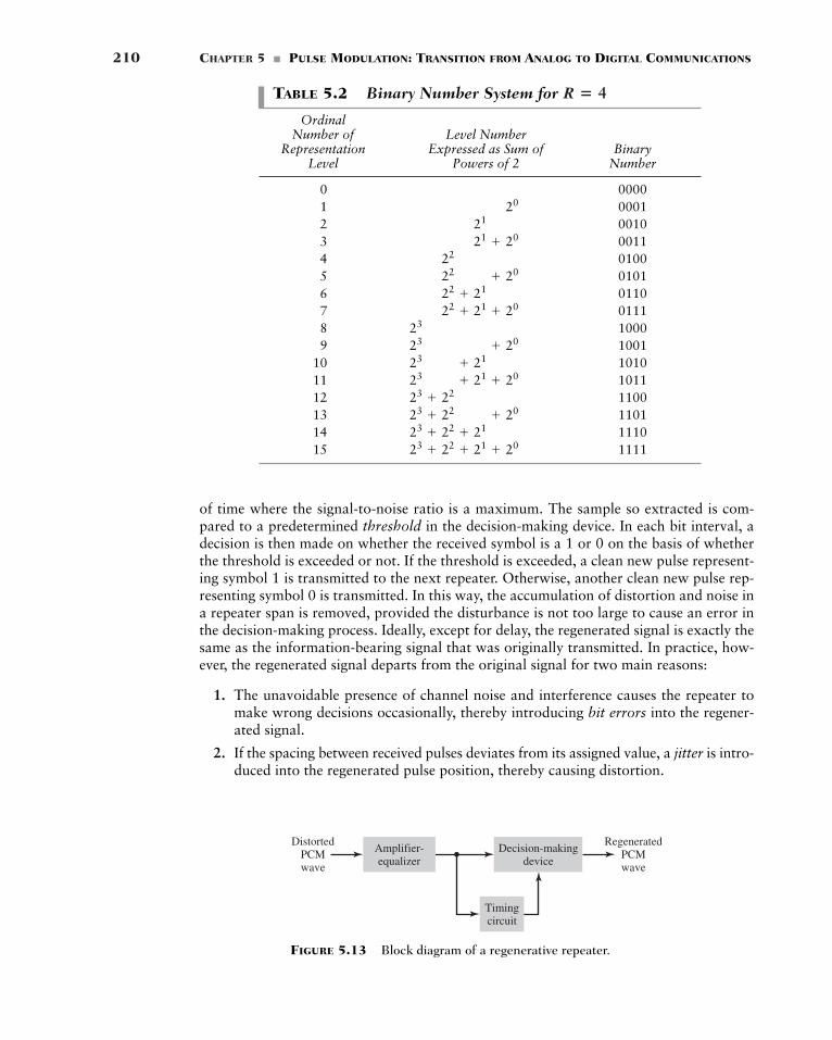
210 CHAPTER 5 � PULSE MODULATION: TRANSITION FROM ANALOG TO DIGITAL COMMUNICATIONS
TABLE 5.2 Binary Number System for
OrdinalNumber of Level Number
Representation Expressed as Sum of BinaryLevel Powers of 2 Number
0 00001 00012 00103 00114 01005 01016 01107 01118 10009 1001
10 101011 101112 110013 110114 111015 111123 22 21 20
23 22 2123 22 2023 2223 21 2023 2123 2023
22 21 2022 2122 2022
21 2021
20
R � 4
of time where the signal-to-noise ratio is a maximum. The sample so extracted is com-pared to a predetermined threshold in the decision-making device. In each bit interval, adecision is then made on whether the received symbol is a 1 or 0 on the basis of whetherthe threshold is exceeded or not. If the threshold is exceeded, a clean new pulse represent-ing symbol 1 is transmitted to the next repeater. Otherwise, another clean new pulse rep-resenting symbol 0 is transmitted. In this way, the accumulation of distortion and noise ina repeater span is removed, provided the disturbance is not too large to cause an error inthe decision-making process. Ideally, except for delay, the regenerated signal is exactly thesame as the information-bearing signal that was originally transmitted. In practice, how-ever, the regenerated signal departs from the original signal for two main reasons:
1. The unavoidable presence of channel noise and interference causes the repeater tomake wrong decisions occasionally, thereby introducing bit errors into the regener-ated signal.
2. If the spacing between received pulses deviates from its assigned value, a jitter is intro-duced into the regenerated pulse position, thereby causing distortion.
Amplifier-equalizer
Decision-makingdevice
Timingcircuit
DistortedPCMwave
RegeneratedPCMwave
FIGURE 5.13 Block diagram of a regenerative repeater.
5.7 Delta Modulation 211
� OPERATIONS IN THE RECEIVER
(i) Decoding and ExpandingThe first operation in the receiver is to regenerate (i.e., reshape and clean up) thereceived pulses one last time. These clean pulses are then regrouped into code wordsand decoded (i.e., mapped back) into a quantized PAM signal. The decoding processinvolves generating a pulse whose amplitude is the linear sum of all the pulses in thecode word; each pulse is weighted by its place value in thecode, where R is the number of bits per sample.
The sequence of decoded samples represents an estimate of the sequence ofcompressed samples produced by the quantizer in the transmitter. We use the term“estimate” here to emphasize the fact that there is no way for the receiver to com-pensate for the approximation introduced into the transmitted signal by the quantizer.Moreover, other sources of noise include bit errors and jitter produced along thetransmission path. In order to restore the sequence of decoded samples to their cor-rect relative level, we must, of course, use a subsystem in the receiver with a charac-teristic complementary to the compressor, used in the transmitter. Such a subsystemis called an expander. Ideally, the compression and expansion laws are exactly inverseso that, except for the effect of quantization, the expander output is equal to the com-pressor input if these two devices were connected directly. The combination of a com-pressor and an expander is referred to as a compander.
(ii) ReconstructionThe final operation in the receiver is to recover the message signal. This operation isachieved by passing the expander output through a low-pass reconstruction filterwhose cutoff frequency is equal to the message bandwidth. Recovery of the messagesignal is intended to signify estimation rather than exact reconstruction.
One last comment is in order. The term “modulation” in pulse-code modulation is a mis-nomer. In reality, pulse-code modulation is a source-encoding strategy, by means of which ananalog signal emitted by a source is converted into digital form. Transmission of the digitaldata so produced is another topic, the treatment of which is deferred to Chapter 6.
5.7 Delta Modulation
From the discussion presented in Section 5.6, it is apparent that the design of a pulse-codemodulation system involves many operations, which tend to make its practical implemen-tation rather costly. To simplify the system design, we may use another digital pulse mod-ulation technique known as delta modulation, which is considered in this section.
� BASIC CONSIDERATIONS
In delta modulation (DM), an incoming message signal is oversampled (i.e., at a rate muchhigher than the Nyquist rate) to purposely increase the correlation between adjacent sam-ples of the signal. The increased correlation is done so as to permit the use of a simplequantizing strategy for constructing the encoded signal.
In its basic form, DM provides a staircase approximation to the oversampled version ofthe message signal. Unlike PCM, the difference between the input signal and its approxima-tion is quantized into only two levels—namely, corresponding to positive and negative dif-ferences. Thus, if the approximation falls below the input signal at any sampling epoch, it isincreased by If, on the other hand, the approximation lies above the signal, it is diminished¢.
�¢,
120, 21, 22, 23, Á , 2R�12
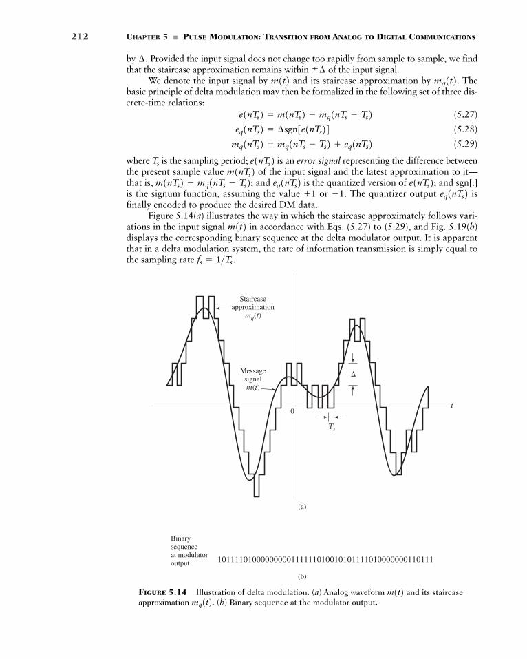
212 CHAPTER 5 � PULSE MODULATION: TRANSITION FROM ANALOG TO DIGITAL COMMUNICATIONS
by Provided the input signal does not change too rapidly from sample to sample, we findthat the staircase approximation remains within of the input signal.
We denote the input signal by and its staircase approximation by Thebasic principle of delta modulation may then be formalized in the following set of three dis-crete-time relations:
(5.27)
(5.28)
(5.29)
where is the sampling period; is an error signal representing the difference betweenthe present sample value of the input signal and the latest approximation to it—that is, and is the quantized version of and sgn[.]is the signum function, assuming the value or The quantizer output isfinally encoded to produce the desired DM data.
Figure 5.14(a) illustrates the way in which the staircase approximately follows vari-ations in the input signal in accordance with Eqs. (5.27) to (5.29), and Fig. 5.19(b)displays the corresponding binary sequence at the delta modulator output. It is apparentthat in a delta modulation system, the rate of information transmission is simply equal tothe sampling rate fs � 1>Ts .
m1t2eq1nTs2�1.1
e1nTs2;eq1nTs2m1nTs2 � mq1nTs � Ts2;m1nTs2e1nTs2Ts
mq1nTs2 � mq1nTs � Ts2 eq1nTs2eq1nTs2 � ¢sgn3e1nTs24e1nTs2 � m1nTs2 � mq1nTs � Ts2
mq1t2.m1t2 �¢¢.
(a)
(b)
Binarysequenceat modulatoroutput 10111101000000000111111010010101111010000000110111
0
Ts
�
Staircaseapproximation
mq(t)
Messagesignalm(t)
t
FIGURE 5.14 Illustration of delta modulation. (a) Analog waveform and its staircaseapproximation (b) Binary sequence at the modulator output.mq1t2. m1t2
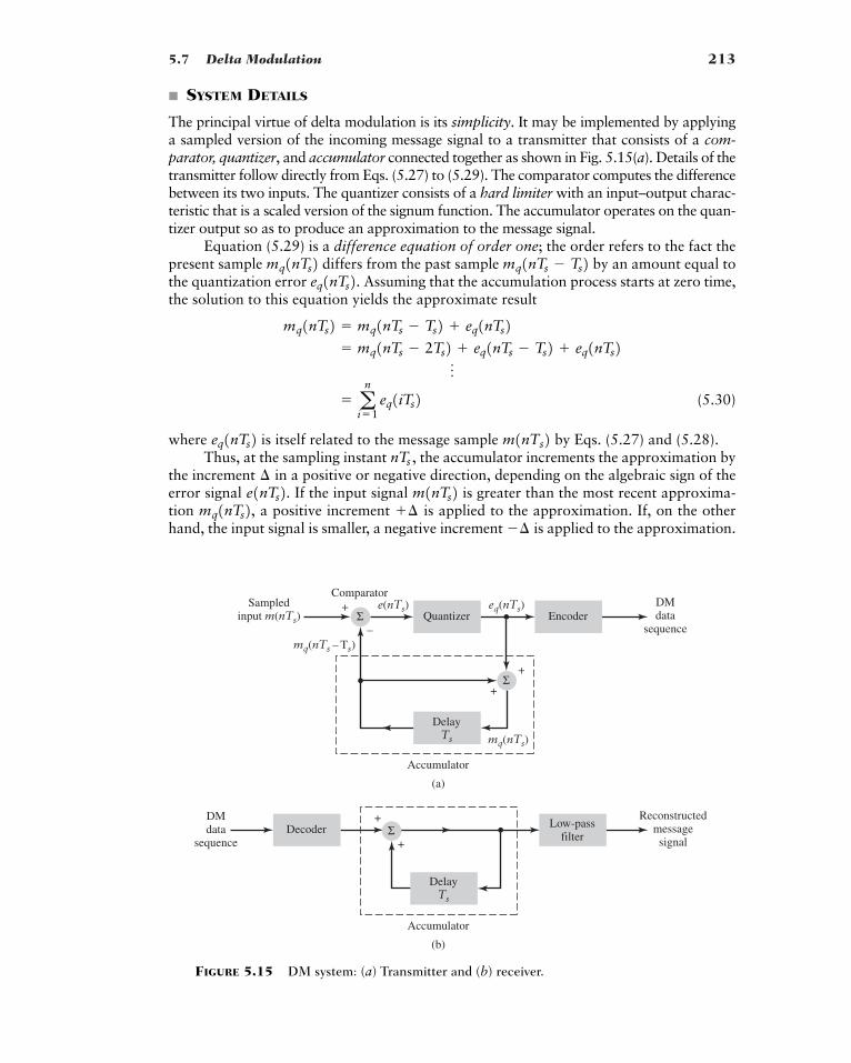
5.7 Delta Modulation 213
� SYSTEM DETAILS
The principal virtue of delta modulation is its simplicity. It may be implemented by applyinga sampled version of the incoming message signal to a transmitter that consists of a com-parator, quantizer, and accumulator connected together as shown in Fig. 5.15(a). Details of thetransmitter follow directly from Eqs. (5.27) to (5.29). The comparator computes the differencebetween its two inputs. The quantizer consists of a hard limiter with an input–output charac-teristic that is a scaled version of the signum function. The accumulator operates on the quan-tizer output so as to produce an approximation to the message signal.
Equation (5.29) is a difference equation of order one; the order refers to the fact thepresent sample differs from the past sample by an amount equal tothe quantization error Assuming that the accumulation process starts at zero time,the solution to this equation yields the approximate result
(5.30)
where is itself related to the message sample by Eqs. (5.27) and (5.28).Thus, at the sampling instant the accumulator increments the approximation by
the increment in a positive or negative direction, depending on the algebraic sign of theerror signal If the input signal is greater than the most recent approxima-tion a positive increment is applied to the approximation. If, on the otherhand, the input signal is smaller, a negative increment is applied to the approximation.�¢
¢mq1nTs2, m1nTs2e1nTs2.¢nTs ,
m1nTs2eq1nTs2� a
n
i�1eq1iTs2
o� mq1nTs � 2Ts2 eq1nTs � Ts2 eq1nTs2
mq1nTs2 � mq1nTs � Ts2 eq1nTs2eq1nTs2. mq1nTs � Ts2mq1nTs2
(a)
e(nTs) eq(nTs)Sampledinput m(nTs)
mq(nTs – Ts)
mq(nTs)
Quantizer
Accumulator
DelayTs
EncoderDMdata
sequence
Comparator+
+
+
–Σ
Σ
(b)
Decoder Low-passfilter
DelayTs
DMdata
sequence
Reconstructedmessagesignal
+
+Σ
Accumulator
FIGURE 5.15 DM system: (a) Transmitter and (b) receiver.
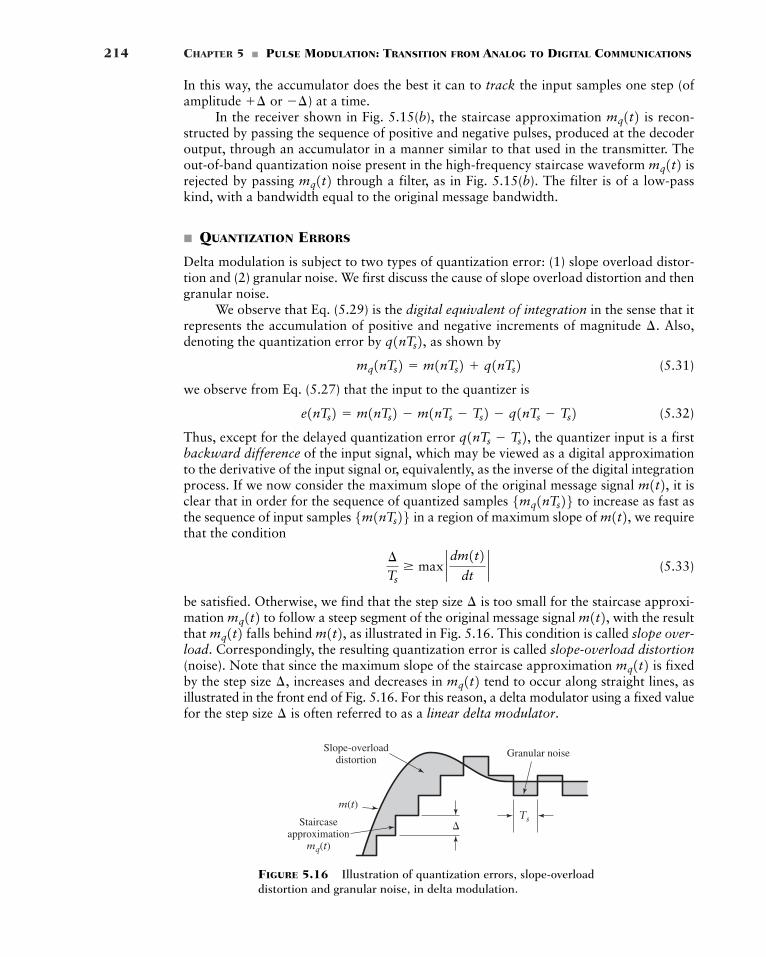
214 CHAPTER 5 � PULSE MODULATION: TRANSITION FROM ANALOG TO DIGITAL COMMUNICATIONS
In this way, the accumulator does the best it can to track the input samples one step (ofamplitude or ) at a time.
In the receiver shown in Fig. 5.15(b), the staircase approximation is recon-structed by passing the sequence of positive and negative pulses, produced at the decoderoutput, through an accumulator in a manner similar to that used in the transmitter. Theout-of-band quantization noise present in the high-frequency staircase waveform isrejected by passing through a filter, as in Fig. 5.15(b). The filter is of a low-passkind, with a bandwidth equal to the original message bandwidth.
� QUANTIZATION ERRORS
Delta modulation is subject to two types of quantization error: (1) slope overload distor-tion and (2) granular noise. We first discuss the cause of slope overload distortion and thengranular noise.
We observe that Eq. (5.29) is the digital equivalent of integration in the sense that itrepresents the accumulation of positive and negative increments of magnitude Also,denoting the quantization error by as shown by
(5.31)
we observe from Eq. (5.27) that the input to the quantizer is
(5.32)
Thus, except for the delayed quantization error the quantizer input is a firstbackward difference of the input signal, which may be viewed as a digital approximationto the derivative of the input signal or, equivalently, as the inverse of the digital integrationprocess. If we now consider the maximum slope of the original message signal it isclear that in order for the sequence of quantized samples to increase as fast asthe sequence of input samples in a region of maximum slope of we requirethat the condition
(5.33)
be satisfied. Otherwise, we find that the step size is too small for the staircase approxi-mation to follow a steep segment of the original message signal with the resultthat falls behind as illustrated in Fig. 5.16. This condition is called slope over-load. Correspondingly, the resulting quantization error is called slope-overload distortion(noise). Note that since the maximum slope of the staircase approximation is fixedby the step size increases and decreases in tend to occur along straight lines, asillustrated in the front end of Fig. 5.16. For this reason, a delta modulator using a fixed valuefor the step size is often referred to as a linear delta modulator.¢
mq1t2¢,mq1t2
m1t2,mq1t2 m1t2,mq1t2 ¢
¢Ts
� max ` dm1t2dt`
m1t2,5m1nTs26 5mq1nTs26 m1t2,q1nTs � Ts2,
e1nTs2 � m1nTs2 � m1nTs � Ts2 � q1nTs � Ts2mq1nTs2 � m1nTs2 q1nTs2
q1nTs2, ¢.
mq1t2 mq1t2mq1t2�¢¢
Slope-overloaddistortion
Granular noise
Staircaseapproximation
mq(t)
Ts�
m(t)
FIGURE 5.16 Illustration of quantization errors, slope-overloaddistortion and granular noise, in delta modulation.
5.7 Delta Modulation 215
4In statistical terms, the average power of a random process (exemplified by quantization error) is equal to themean-square value of that process; this issue is discussed in Chapter 8.
In contrast to slope-overload distortion, granular noise occurs when the step size istoo large relative to the local slope characteristic of the original message signal Thissecond situation causes the staircase approximation to hunt around a relatively flatsegment of which is illustrated in the back end of Fig. 5.16. Granular noise in deltamodulation may be viewed as the analog of quantization noise in pulse-code modulation.
� Drill Problem 5.10 The best that a linear DM system can do is to provide a compro-mise between slope-overload distortion and granular noise. Justify this statement. �
From this discussion we see that there is a need to have a large step size to accom-modate a wide dynamic range, whereas a small step size is required for the accurate rep-resentation of relatively low-level signals. It is therefore clear that if we are to choose anoptimum step size that minimizes the average power4 of the quantization error in a deltamodulator, we need to make the DM system adaptive. This requirement, in turn, means thatthe step size has to vary in accordance with the incoming message signal.
� DELTA-SIGMA MODULATION
As mentioned previously, the quantizer input in the conventional form of delta modulationmay be viewed as an approximation to the derivative of the incoming message signal. Thisbehavior leads to a drawback of delta modulation in that transmission disturbances suchas noise result in an accumulative error in the demodulated signal. This drawback can beovercome by integrating the message signal prior to delta modulation. The use of integra-tion also has other beneficial effects:
� The low-frequency content of the input signal is pre-emphasized.� Correlation between adjacent samples of the delta modulator input is increased, which
tends to improve overall system performance by reducing the average power of theerror signal at the quantizer input.
� Design of the receiver is simplified.
A delta modulation system that incorporates integration at its input is called delta-sigma modulation To be more precise, however, it should be called sigma-deltamodulation, because the integration is in fact performed before the delta modulation. Nev-ertheless, the former terminology is the one commonly used in the literature.
Figure 5.17(a) shows the block diagram of a delta-sigma modulation system. In thisdiagram, the message signal is defined in its continuous-time form, which means thatthe pulse modulator now consists of a hard-limiter followed by a multiplier; the latter com-ponent is also fed from an external pulse generator (clock) to produce a 1-bit encoded sig-nal. The use of integration at the transmitter input clearly requires an inverse signalemphasis—namely, differentiation—at the receiver. The need for this differentiation is,however, eliminated because of its cancellation by integration in the conventional DMreceiver. Thus, the receiver of a delta-sigma modulation system consists simply of a low-pass filter, as indicated in Fig. 5.17(a).
Moreover, we note that integration is basically a linear operation. Accordingly, we maysimplify the design of the transmitter by combining the two integrators 1 and 2 of Fig. 5.17(a) into a single integrator placed after the comparator, as shown in Fig. 5.17(b).
m1t2
1D-©M2.
m1t2, mq1t2 m1t2. ¢
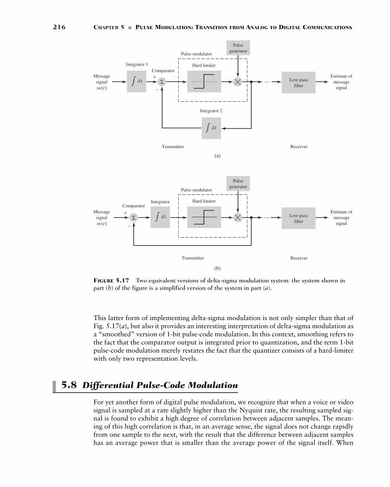
216 CHAPTER 5 � PULSE MODULATION: TRANSITION FROM ANALOG TO DIGITAL COMMUNICATIONS
This latter form of implementing delta-sigma modulation is not only simpler than that ofFig. 5.17(a), but also it provides an interesting interpretation of delta-sigma modulation asa “smoothed” version of 1-bit pulse-code modulation. In this context, smoothing refers tothe fact that the comparator output is integrated prior to quantization, and the term 1-bitpulse-code modulation merely restates the fact that the quantizer consists of a hard-limiterwith only two representation levels.
5.8 Differential Pulse-Code Modulation
For yet another form of digital pulse modulation, we recognize that when a voice or videosignal is sampled at a rate slightly higher than the Nyquist rate, the resulting sampled sig-nal is found to exhibit a high degree of correlation between adjacent samples. The mean-ing of this high correlation is that, in an average sense, the signal does not change rapidlyfrom one sample to the next, with the result that the difference between adjacent sampleshas an average power that is smaller than the average power of the signal itself. When
Hard limiter
Messagesignalm(t)
Estimate ofmessagesignal
Low-passfilter
Integrator 2
dt∫Comparator
...
Transmitter Receiver
+
Pulsegenerator
Hard limiter
Messagesignalm(t)
Estimate ofmessagesignal
Low-passfilter
Integrator
dt∫Comparator
...
Transmitter Receiver
+
Pulsegenerator
Pulse modulator
Pulse modulator
(a)
(b)
–
dt∫
Integrator 1
–
Σ
Σ
FIGURE 5.17 Two equivalent versions of delta-sigma modulation system: the system shown inpart (b) of the figure is a simplified version of the system in part (a).
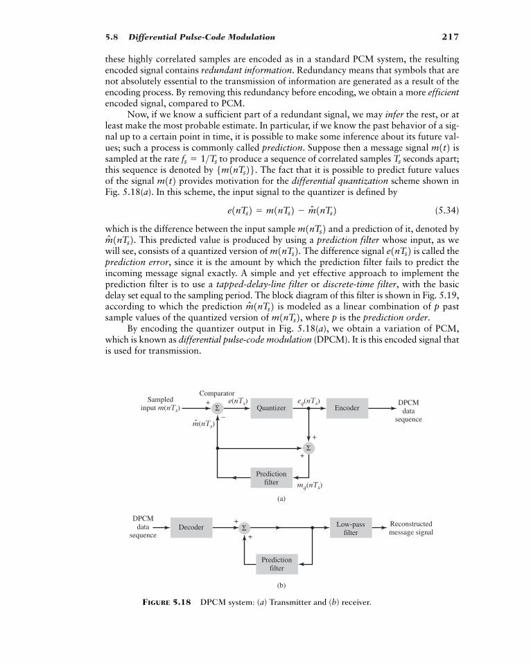
5.8 Differential Pulse-Code Modulation 217
these highly correlated samples are encoded as in a standard PCM system, the resultingencoded signal contains redundant information. Redundancy means that symbols that arenot absolutely essential to the transmission of information are generated as a result of theencoding process. By removing this redundancy before encoding, we obtain a more efficientencoded signal, compared to PCM.
Now, if we know a sufficient part of a redundant signal, we may infer the rest, or atleast make the most probable estimate. In particular, if we know the past behavior of a sig-nal up to a certain point in time, it is possible to make some inference about its future val-ues; such a process is commonly called prediction. Suppose then a message signal issampled at the rate to produce a sequence of correlated samples seconds apart;this sequence is denoted by The fact that it is possible to predict future valuesof the signal provides motivation for the differential quantization scheme shown inFig. 5.18(a). In this scheme, the input signal to the quantizer is defined by
(5.34)
which is the difference between the input sample and a prediction of it, denoted byThis predicted value is produced by using a prediction filter whose input, as we
will see, consists of a quantized version of The difference signal is called theprediction error, since it is the amount by which the prediction filter fails to predict theincoming message signal exactly. A simple and yet effective approach to implement theprediction filter is to use a tapped-delay-line filter or discrete-time filter, with the basicdelay set equal to the sampling period. The block diagram of this filter is shown in Fig. 5.19,according to which the prediction is modeled as a linear combination of p pastsample values of the quantized version of where p is the prediction order.
By encoding the quantizer output in Fig. 5.18(a), we obtain a variation of PCM,which is known as differential pulse-code modulation (DPCM). It is this encoded signal thatis used for transmission.
m1nTs2,mN 1nTs2
e1nTs2m1nTs2.mN 1nTs2. m1nTs2e1nTs2 � m1nTs2 � mN 1nTs2
m1t2 5m1nTs26. Tsfs � 1>Ts
m1t2
(a)
e(nTs) eq(nTs)Sampledinput m(nTs)
m(nTs)n
mq(nTs)
Quantizer
Predictionfilter
EncoderDPCM
datasequence
Comparator+
+
+
–Σ
Σ
(b)
Decoder Low-passfilter
Predictionfilter
DPCMdata
sequence
Reconstructedmessage signal
+
+Σ
FIGURE 5.18 DPCM system: (a) Transmitter and (b) receiver.
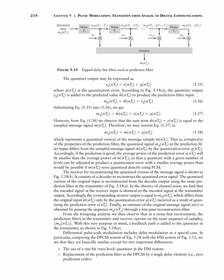
218 CHAPTER 5 � PULSE MODULATION: TRANSITION FROM ANALOG TO DIGITAL COMMUNICATIONS
m(nTs)
Quantizedinput
mq(nTs)
mq(nTs – Ts)
Summer
w1 w2
mq(nTs – 2Ts)
wp–1
mq(nTs – pTs + Ts) mq(nTs – pTs)
wp
DelayTs
DelayTs
DelayTs
...
FIGURE 5.19 Tapped-delay line filter used as prediction filter.
The quantizer output may be expressed as
(5.35)
where is the quantization error. According to Fig. 5.18(a), the quantizer outputis added to the predicted value to produce the prediction-filter input
(5.36)
Substituting Eq. (5.35) into (5.36), we get
(5.37)
However, from Eq. (5.34) we observe that the sum term is equal to thesampled message signal Therefore, we may rewrite Eq. (5.37) as
(5.38)
which represents a quantized version of the message sample That is, irrespectiveof the properties of the prediction filter, the quantized signal at the prediction fil-ter input differs from the sampled message signal by the quantization error Accordingly, if the prediction is good, the average power of the prediction error willbe smaller than the average power of so that a quantizer with a given number oflevels can be adjusted to produce a quantization error with a smaller average power thanwould be possible if were quantized directly using PCM.
The receiver for reconstructing the quantized version of the message signal is shown inFig. 5.18(b). It consists of a decoder to reconstruct the quantized error signal. The quantizedversion of the original input is reconstructed from the decoder output using the same pre-diction filter in the transmitter of Fig. 5.18(a). In the absence of channel noise, we find thatthe encoded signal at the receiver input is identical to the encoded signal at the transmitteroutput. Accordingly, the corresponding receiver output is equal to which differs fromthe original input only by the quantization error incurred as a result of quan-tizing the prediction error Finally, an estimate of the original message signal isobtained by passing the sequence through a low-pass reconstruction filter.
From the foregoing analysis we thus observe that in a noise-free environment, theprediction filters in the transmitter and receiver operate on the same sequence of samples,
With this very purpose in mind, a feedback path is added to the quantizer inthe transmitter, as shown in Fig. 5.18(a).
Differential pulse-code modulation includes delta modulation as a special case. Inparticular, comparing the DPCM system of Fig. 5.18 with the DM system of Fig. 5.15, wesee that they are basically similar, except for two important differences:
� The use of a one-bit (two-level) quantizer in the DM system.� Replacement of the prediction filter in the DPCM by a single delay element (i.e., zero
prediction order).
5mq1nTs26.mq1nTs2 m1t2e1nTs2. q1nTs2m1nTs2 mq1nTs2,
m1nTs2m1nTs2, e1nTs2q1nTs2.m1nTs2 mq1nTs2m1nTs2.
mq1nTs2 � m1nTs2 q1nTs2m1nTs2. mN 1nTs2 e1nTs2mq1nTs2 � mN 1nTs2 e1nTs2 q1nTs2
mq1nTs2 � mN 1nTs2 eq1nTs2mN 1nTs2eq1nTs2q1nTs2
eq1nTs2 � e1nTs2 q1nTs2
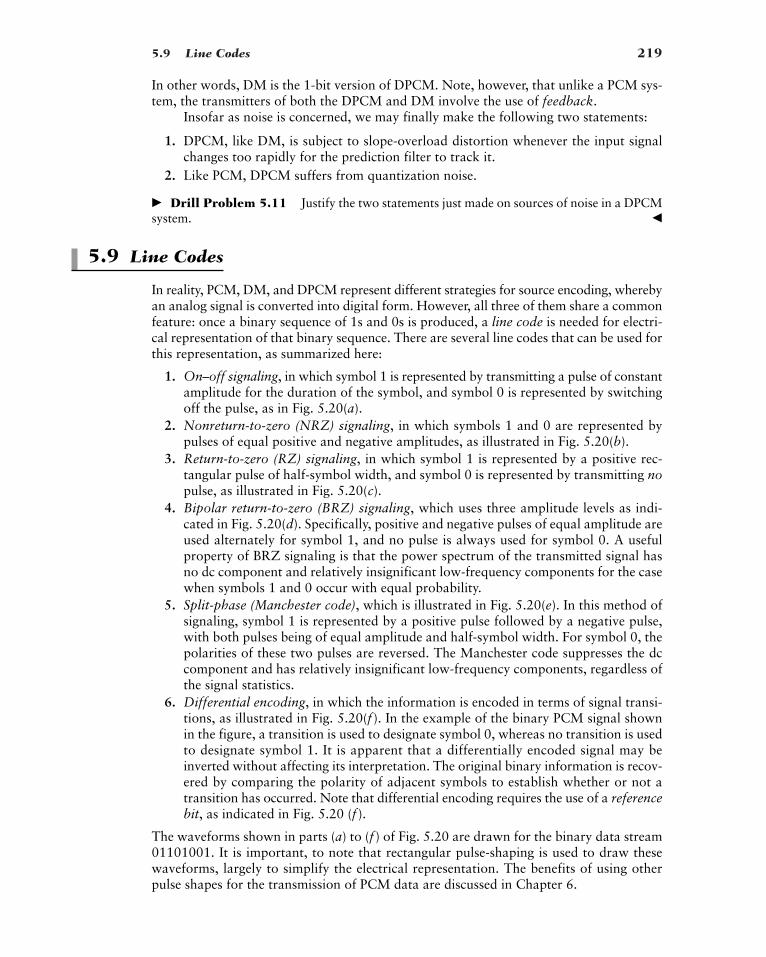
5.9 Line Codes 219
In other words, DM is the 1-bit version of DPCM. Note, however, that unlike a PCM sys-tem, the transmitters of both the DPCM and DM involve the use of feedback.
Insofar as noise is concerned, we may finally make the following two statements:
1. DPCM, like DM, is subject to slope-overload distortion whenever the input signalchanges too rapidly for the prediction filter to track it.
2. Like PCM, DPCM suffers from quantization noise.
� Drill Problem 5.11 Justify the two statements just made on sources of noise in a DPCMsystem. �
5.9 Line Codes
In reality, PCM, DM, and DPCM represent different strategies for source encoding, wherebyan analog signal is converted into digital form. However, all three of them share a commonfeature: once a binary sequence of 1s and 0s is produced, a line code is needed for electri-cal representation of that binary sequence. There are several line codes that can be used forthis representation, as summarized here:
1. On–off signaling, in which symbol 1 is represented by transmitting a pulse of constantamplitude for the duration of the symbol, and symbol 0 is represented by switchingoff the pulse, as in Fig. 5.20(a).
2. Nonreturn-to-zero (NRZ) signaling, in which symbols 1 and 0 are represented bypulses of equal positive and negative amplitudes, as illustrated in Fig. 5.20(b).
3. Return-to-zero (RZ) signaling, in which symbol 1 is represented by a positive rec-tangular pulse of half-symbol width, and symbol 0 is represented by transmitting nopulse, as illustrated in Fig. 5.20(c).
4. Bipolar return-to-zero (BRZ) signaling, which uses three amplitude levels as indi-cated in Fig. 5.20(d). Specifically, positive and negative pulses of equal amplitude areused alternately for symbol 1, and no pulse is always used for symbol 0. A usefulproperty of BRZ signaling is that the power spectrum of the transmitted signal hasno dc component and relatively insignificant low-frequency components for the casewhen symbols 1 and 0 occur with equal probability.
5. Split-phase (Manchester code), which is illustrated in Fig. 5.20(e). In this method ofsignaling, symbol 1 is represented by a positive pulse followed by a negative pulse,with both pulses being of equal amplitude and half-symbol width. For symbol 0, thepolarities of these two pulses are reversed. The Manchester code suppresses the dccomponent and has relatively insignificant low-frequency components, regardless ofthe signal statistics.
6. Differential encoding, in which the information is encoded in terms of signal transi-tions, as illustrated in Fig. 5.20(f ). In the example of the binary PCM signal shownin the figure, a transition is used to designate symbol 0, whereas no transition is usedto designate symbol 1. It is apparent that a differentially encoded signal may beinverted without affecting its interpretation. The original binary information is recov-ered by comparing the polarity of adjacent symbols to establish whether or not atransition has occurred. Note that differential encoding requires the use of a referencebit, as indicated in Fig. 5.20 (f ).
The waveforms shown in parts (a) to (f ) of Fig. 5.20 are drawn for the binary data stream01101001. It is important, to note that rectangular pulse-shaping is used to draw thesewaveforms, largely to simplify the electrical representation. The benefits of using otherpulse shapes for the transmission of PCM data are discussed in Chapter 6.
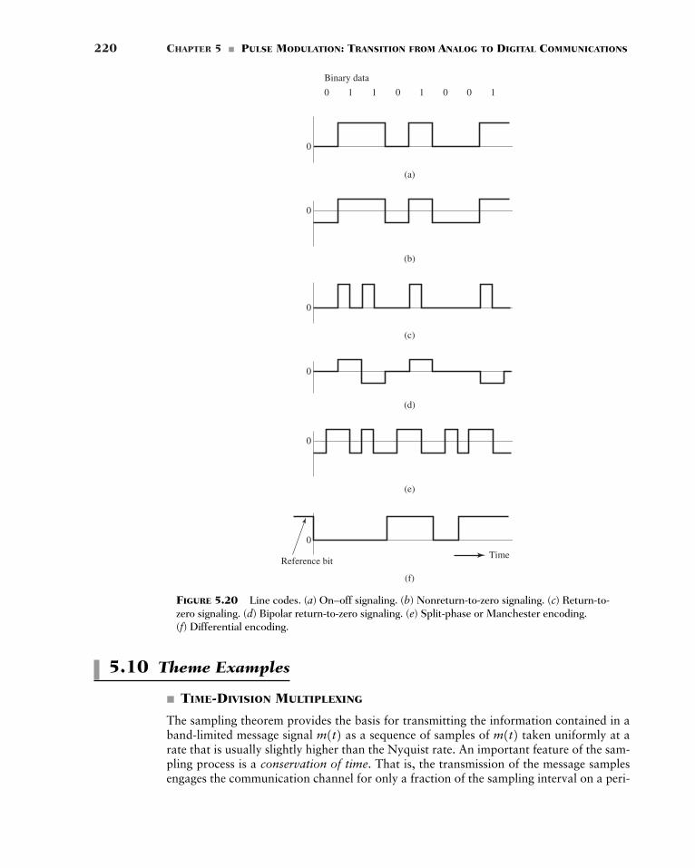
220 CHAPTER 5 � PULSE MODULATION: TRANSITION FROM ANALOG TO DIGITAL COMMUNICATIONS
5.10 Theme Examples
� TIME-DIVISION MULTIPLEXING
The sampling theorem provides the basis for transmitting the information contained in aband-limited message signal as a sequence of samples of taken uniformly at arate that is usually slightly higher than the Nyquist rate. An important feature of the sam-pling process is a conservation of time. That is, the transmission of the message samplesengages the communication channel for only a fraction of the sampling interval on a peri-
m1t2m1t2
Binary data
0 1 1 0 1 0 0 1
(a)
0
(b)
0
(e)
0
(c)
0
(d)
0
(f)
0
TimeReference bit
FIGURE 5.20 Line codes. (a) On–off signaling. (b) Nonreturn-to-zero signaling. (c) Return-to-zero signaling. (d) Bipolar return-to-zero signaling. (e) Split-phase or Manchester encoding. (f) Differential encoding.
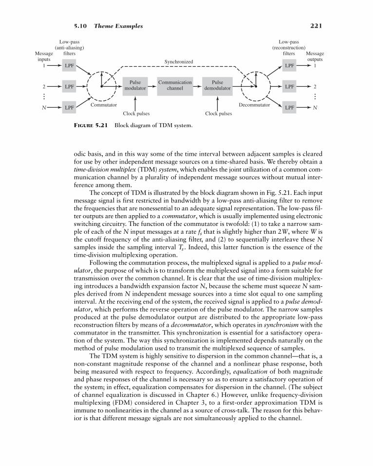
5.10 Theme Examples 221
odic basis, and in this way some of the time interval between adjacent samples is clearedfor use by other independent message sources on a time-shared basis. We thereby obtain atime-division multiplex (TDM) system, which enables the joint utilization of a common com-munication channel by a plurality of independent message sources without mutual inter-ference among them.
The concept of TDM is illustrated by the block diagram shown in Fig. 5.21. Each inputmessage signal is first restricted in bandwidth by a low-pass anti-aliasing filter to removethe frequencies that are nonessential to an adequate signal representation. The low-pass fil-ter outputs are then applied to a commutator, which is usually implemented using electronicswitching circuitry. The function of the commutator is twofold: (1) to take a narrow sam-ple of each of the N input messages at a rate that is slightly higher than 2W, where W isthe cutoff frequency of the anti-aliasing filter, and (2) to sequentially interleave these Nsamples inside the sampling interval Indeed, this latter function is the essence of thetime-division multiplexing operation.
Following the commutation process, the multiplexed signal is applied to a pulse mod-ulator, the purpose of which is to transform the multiplexed signal into a form suitable fortransmission over the common channel. It is clear that the use of time-division multiplex-ing introduces a bandwidth expansion factor N, because the scheme must squeeze N sam-ples derived from N independent message sources into a time slot equal to one samplinginterval. At the receiving end of the system, the received signal is applied to a pulse demod-ulator, which performs the reverse operation of the pulse modulator. The narrow samplesproduced at the pulse demodulator output are distributed to the appropriate low-passreconstruction filters by means of a decommutator, which operates in synchronism with thecommutator in the transmitter. This synchronization is essential for a satisfactory opera-tion of the system. The way this synchronization is implemented depends naturally on themethod of pulse modulation used to transmit the multiplexed sequence of samples.
The TDM system is highly sensitive to dispersion in the common channel—that is, anon-constant magnitude response of the channel and a nonlinear phase response, bothbeing measured with respect to frequency. Accordingly, equalization of both magnitudeand phase responses of the channel is necessary so as to ensure a satisfactory operation ofthe system; in effect, equalization compensates for dispersion in the channel. (The subjectof channel equalization is discussed in Chapter 6.) However, unlike frequency-divisionmultiplexing (FDM) considered in Chapter 3, to a first-order approximation TDM isimmune to nonlinearities in the channel as a source of cross-talk. The reason for this behav-ior is that different message signals are not simultaneously applied to the channel.
Ts .
fs
LPF
Low-pass(anti-aliasing)
filters
Low-pass(reconstruction)
filters
Pulsemodulator
Communicationchannel
Synchronized
Clock pulses Clock pulses
1
Pulsedemodulator
DecommutatorCommutator
LPF2
LPF
LPF
LPF
LPFN
Messageinputs
...
1
2
N
Messageoutputs
...
FIGURE 5.21 Block diagram of TDM system.

222 CHAPTER 5 � PULSE MODULATION: TRANSITION FROM ANALOG TO DIGITAL COMMUNICATIONS
Synchronization
In applications using PCM, for example, it is natural to multiplex different messagessources by time division, whereby each source keeps its distinction from all other sourcesthroughout the journey from the transmitter to the receiver. This individuality accountsfor the comparative ease with which message sources may be dropped or reinserted in a time-division multiplex system. As the number of independent message sources is increased, thetime interval that may be allotted to each source has to be reduced, since all of them mustbe accommodated into a time interval equal to the reciprocal of the sampling rate. This,in turn, means that the allowable duration of a codeword representing a single sample isreduced. However, pulses tend to become more difficult to generate and to transmit astheir duration is reduced. Furthermore, if the pulses become too short, impairments in thetransmission medium begin to interfere with the proper operation of the system. Accord-ingly, in practice, it is necessary to restrict the number of independent message sources thatcan be included within a time-division group.
In any event, for a PCM system with time-division multiplexing to operate satisfac-torily, it is necessary that the timing operations at the receiver, except for the time lost intransmission and regenerative repeating, follow closely the corresponding operations atthe transmitter. In a general way, this amounts to requiring a local clock at the receiver tokeep the same time as a distant standard clock at the transmitter, except that the local clockis delayed by an amount equal to the time required to transport the message signals fromthe transmitter to the receiver. This delay, in turn, gives rise to a phase difference betweenthe two clocks. One possible procedure to synchronize the transmitter and receiver clocksis to set aside a code element or pulse at the end of a frame (consisting of a code wordderived from each of the independent message sources in succession) and to transmit thispulse every other frame only. In such a case, the receiver includes a circuit that would searchfor the pattern of 1s and 0s alternating at half the frame rate, and thereby establish syn-chronization between the transmitter and receiver.
When the transmission path is interrupted, it is highly unlikely that the transmitterand receiver clocks will continue to indicate the same time for long. Accordingly, in carry-ing out a synchronization process, we must set up an orderly procedure for detecting thesynchronizing pulse. The procedure consists of observing the code elements one by oneuntil the synchronizing pulse is detected. That is, after observing a particular code elementlong enough to establish the absence of the synchronizing pulse, the receiver clock is set backby one code element and the next code element is observed. This searching process isrepeated until the synchronizing pulse is detected. Clearly, the time required for synchro-nization depends on the epoch at which proper transmission is re-established.
EXAMPLE 5.1 The T1 System
In this example, we describe the important characteristics of a PCM system known as the T1system, which carries 24 voice channels over pairs of wires with regenerative repeaters spacedat approximately 2-km intervals. The T1 carrier system is basic to the North American digi-tal switching hierarchy5 for telephonic communication.
A voice signal (male or female) is essentially limited to a band from 300 to 3100 Hzin that frequencies outside this band do not contribute much to voice recognition andcomprehension. Indeed, telephone circuits that respond to this range of frequencies give
5For a description of the digital switching hierarchy used in North America, see Haykin (2001), pp. 214–217.
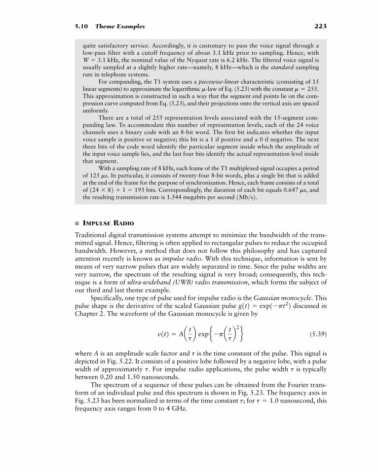
5.10 Theme Examples 223
quite satisfactory service. Accordingly, it is customary to pass the voice signal through alow-pass filter with a cutoff frequency of about 3.1 kHz prior to sampling. Hence, with
the nominal value of the Nyquist rate is 6.2 kHz. The filtered voice signal isusually sampled at a slightly higher rate—namely, 8 kHz—which is the standard samplingrate in telephone systems.
For companding, the T1 system uses a piecewise-linear characteristic (consisting of 15linear segments) to approximate the logarithmic of Eq. (5.23) with the constant This approximation is constructed in such a way that the segment end points lie on the com-pression curve computed from Eq. (5.23), and their projections onto the vertical axis are spaceduniformly.
There are a total of 255 representation levels associated with the 15-segment com-panding law. To accommodate this number of representation levels, each of the 24 voicechannels uses a binary code with an 8-bit word. The first bit indicates whether the inputvoice sample is positive or negative; this bit is a 1 if positive and a 0 if negative. The nextthree bits of the code word identify the particular segment inside which the amplitude ofthe input voice sample lies, and the last four bits identify the actual representation level insidethat segment.
With a sampling rate of 8 kHz, each frame of the T1 multiplexed signal occupies a periodof In particular, it consists of twenty-four 8-bit words, plus a single bit that is addedat the end of the frame for the purpose of synchronization. Hence, each frame consists of a totalof bits. Correspondingly, the duration of each bit equals andthe resulting transmission rate is 1.544 megabits per second
� IMPULSE RADIO
Traditional digital transmission systems attempt to minimize the bandwidth of the trans-mitted signal. Hence, filtering is often applied to rectangular pulses to reduce the occupiedbandwidth. However, a method that does not follow this philosophy and has capturedattention recently is known as impulse radio. With this technique, information is sent bymeans of very narrow pulses that are widely separated in time. Since the pulse widths arevery narrow, the spectrum of the resulting signal is very broad; consequently, this tech-nique is a form of ultra-wideband (UWB) radio transmission, which forms the subject ofour third and last theme example.
Specifically, one type of pulse used for impulse radio is the Gaussian monocycle. Thispulse shape is the derivative of the scaled Gaussian pulse discussed inChapter 2. The waveform of the Gaussian monocycle is given by
(5.39)
where A is an amplitude scale factor and is the time constant of the pulse. This signal isdepicted in Fig. 5.22. It consists of a positive lobe followed by a negative lobe, with a pulsewidth of approximately For impulse radio applications, the pulse width is typicallybetween 0.20 and 1.50 nanoseconds.
The spectrum of a sequence of these pulses can be obtained from the Fourier trans-form of an individual pulse and this spectrum is shown in Fig. 5.23. The frequency axis inFig. 5.23 has been normalized in terms of the time constant for nanosecond, thisfrequency axis ranges from 0 to 4 GHz.
t � 1.0t;
tt.
t
v1t2 � Aa ttb expe�pa t
tb2 f
g1t2 � exp1�pt22
1Mb>s2. 0.647 ms,124 82 1 � 193
125 ms.
m � 255.m-law
W � 3.1 kHz,
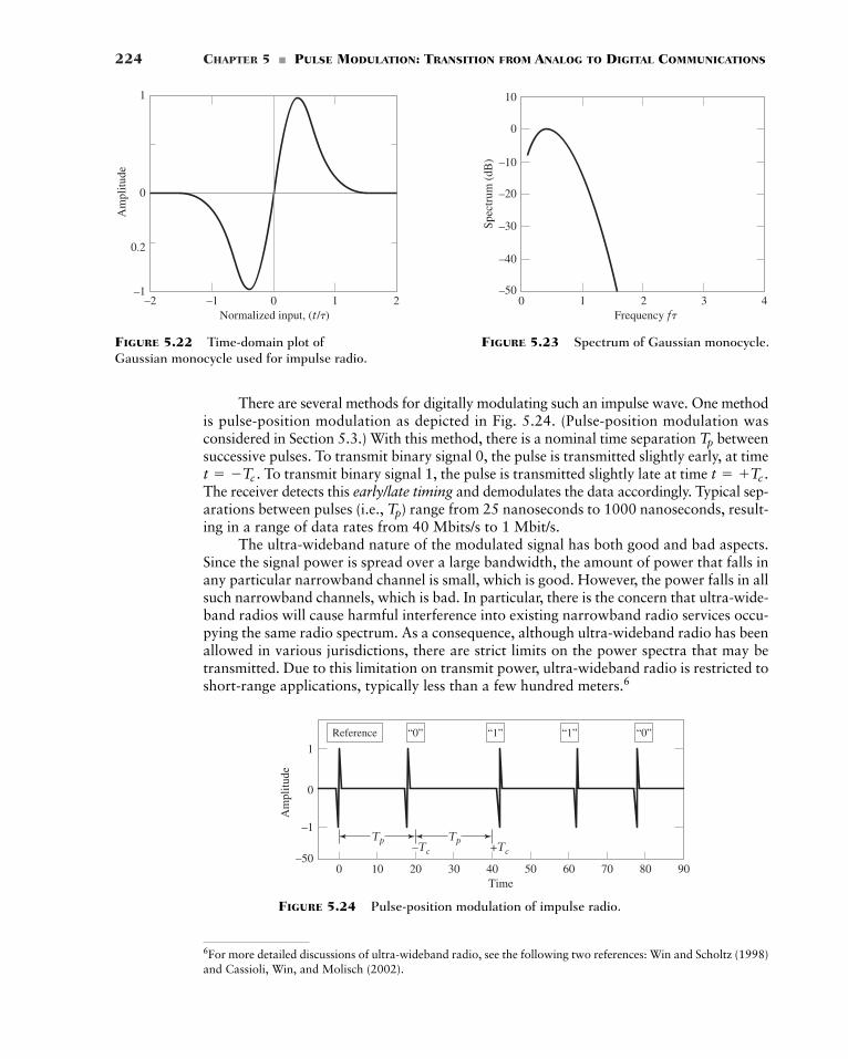
224 CHAPTER 5 � PULSE MODULATION: TRANSITION FROM ANALOG TO DIGITAL COMMUNICATIONS
–2 –1Normalized input, (t/�)
0 1 2–1
0.2
0
1
Am
plitu
de
FIGURE 5.22 Time-domain plot ofGaussian monocycle used for impulse radio.
0 1Frequency f�
2 3 4–50
–40
–30
–20
–10
0
10
Spec
trum
(dB
)
FIGURE 5.23 Spectrum of Gaussian monocycle.
0Time
Reference
10
Tp–Tc +Tc
20 30 40 50 60 70 80 90–50
–1
0
1
Am
plitu
de
“0” “0”“1” “1”
Tp
FIGURE 5.24 Pulse-position modulation of impulse radio.
6For more detailed discussions of ultra-wideband radio, see the following two references: Win and Scholtz (1998)and Cassioli, Win, and Molisch (2002).
There are several methods for digitally modulating such an impulse wave. One methodis pulse-position modulation as depicted in Fig. 5.24. (Pulse-position modulation wasconsidered in Section 5.3.) With this method, there is a nominal time separation betweensuccessive pulses. To transmit binary signal 0, the pulse is transmitted slightly early, at time
To transmit binary signal 1, the pulse is transmitted slightly late at time The receiver detects this early/late timing and demodulates the data accordingly. Typical sep-arations between pulses (i.e., ) range from 25 nanoseconds to 1000 nanoseconds, result-ing in a range of data rates from 40 Mbits/s to 1 Mbit/s.
The ultra-wideband nature of the modulated signal has both good and bad aspects.Since the signal power is spread over a large bandwidth, the amount of power that falls inany particular narrowband channel is small, which is good. However, the power falls in allsuch narrowband channels, which is bad. In particular, there is the concern that ultra-wide-band radios will cause harmful interference into existing narrowband radio services occu-pying the same radio spectrum. As a consequence, although ultra-wideband radio has beenallowed in various jurisdictions, there are strict limits on the power spectra that may betransmitted. Due to this limitation on transmit power, ultra-wideband radio is restricted toshort-range applications, typically less than a few hundred meters.6
Tp
t � Tc .t � �Tc .
Tp
5.11 Summary and Discussion 225
5.11 Summary and Discussion
In this chapter, we introduced two fundamental and complementary processes:
� Sampling, which operates in the time domain; the sampling process is the link betweenan analog waveform and its discrete-time representation.
� Quantization, which operates in the amplitude domain; the quantization process isthe link between an analog waveform and its discrete-amplitude representation.
The sampling process builds on the sampling theorem, which states that a strictly band-lim-ited signal with no frequency components higher than W Hz is represented uniquely by asequence of samples taken at a uniform rate equal to or greater than the Nyquist rate of2W samples per second. As for the quantization process it exploits the fact that any humansense, as ultimate receiver, can only detect finite intensity differences.
The sampling process is basic to the operation of all pulse modulation systems, whichmay be classified into analog pulse modulation and digital pulse modulation. The distin-guishing feature between them is that analog pulse modulation systems maintain a con-tinuous amplitude representation of the message signal, whereas digital pulse modulationsystems employ quantization to provide a representation of the message signal that isdiscrete in both time and amplitude.
Analog pulse modulation results from varying some parameter of the transmittedpulses, such as amplitude, duration, or position, in which case we speak of pulse-amplitudemodulation (PAM), pulse-duration modulation (PDM), or pulse-position modulation (PPM),respectively.
Digital pulse modulation systems, on the other hand, transmit analog message signalsas a sequence of coded pulses, which is made possible through the combined use of sam-pling and quantization. Pulse-code modulation is a form of digital pulse modulation thatis endowed with some unique system advantages, which, in turn, have made it the pre-ferred method of encoding for the transmission of such analog signals as voice and videosignals. The advantages of pulse-code modulation include robustness to noise and inter-ference, efficient regeneration of the encoded pulses along the transmission path, and auniform format for different kinds of message signals. (i.e. voice, video, and data).
Delta modulation and differential pulse-code modulation are two other useful formsof digital pulse modulation. The principal advantage of delta modulation is simplified cir-cuitry. However, this advantage is gained at the expense of increased data transmissionrate. In contrast, differential pulse-code modulation employs increased circuit complexityto improve system performance. The improvement is achieved at the expense of increasedsystem complexity, which facilitates the idea of prediction to remove redundant symbolsfrom the incoming data stream, and thereby permit the use of reduced channel bandwidthcompared to PCM.
Further improvements in the operations of delta modulation and differential pulse-code modulation can be made through the use of adaptivity to account for statistical vari-ations in the input data. Specifically, adaptivity is used in delta modulation to improvenoise performance. On the other hand, adaptivity is used in differential pulse-code modu-lation to reduce bandwidth requirement.
It is important to recognize that pulse modulation techniques are lossy in the sense thatsome information is lost as a result of the signal representation that they perform. For exam-ple, in pulse-amplitude modulation, the customary practice is to use anti-alias (low-pass) fil-tering prior to sampling; in so doing, information is lost by virtue of the fact that high-frequencycomponents considered to be unessential are removed by the filter. The lossy nature of pulsemodulation is most vividly seen in pulse-code modulation that is impaired by quantization
226 CHAPTER 5 � PULSE MODULATION: TRANSITION FROM ANALOG TO DIGITAL COMMUNICATIONS
noise (i.e., distortion), which arises because the transmitted sequence of encoded pulses doesnot have the infinite precision needed to represent continuous samples exactly. Nevertheless,the loss of information incurred by the use of a pulse modulation process is under the designer’scontrol, in that it can be made small enough for it to be nondiscernible by the end user.
A point that needs to be stressed one last time: In reality, PCM, DM, and DPCM aresource-encoding strategies, whose purpose is to convert analog signals into digital form. Foractual transmission of the encoded data over a communication channel, the discrete formof pulse-amplitude modulation (PAM) is typically used. (Details of this application of PAMare presented in the next chapter).
In the chapter, we also included three theme examples, addressing important appli-cations summarized here:
� Time-division multiplexing, which enables the joint utilization of a communicationchannel by a multitude of independent message sources by building on an importantfeature of the sampling process—namely, the conservation of time.
� The T1 system, which accommodates the PCM transmission of 24 voice channels overpairs of wires with regenerative repeaters spaced at approximately 2-km intervals.
� Impulse radio, by means of which information is sent across a wireless channel at base-band, using very narrow pulses.
ADDITIONAL PROBLEMS
5.12 (a) Plot the spectrum of a PAM wave produced by the modulating signal
assuming the modulation frequency sampling period and pulseduration
(b) Using an ideal reconstruction filter, plot the spectrum of the filter output. Compare thisresult with the output that would be obtained if there were no aperture effect.
5.13 In this problem, we evaluate the equalization needed for the aperture effect in a PAM system.The operating frequency which corresponds to the highest frequency component of themessage signal for a sampling rate equal to the Nyquist rate. Plot versus and hence find the equalization needed when
5.14 A PAM telemetry system involves the multiplexing of four input signals: Two of the signals and have bandwidths of 80 Hz each, whereas the remaining twosignals and have bandwidths of 1 kHz each. The signals and are each sam-pled at the rate of 2400 samples per second. This sampling rate is divided by (i.e., an inte-ger power of 2) in order to derive the sampling rate for and (a) Find the maximum value of R.(b) Using the value of R found in part (a), design a multiplexing system that first multiplexes
and into a new sequence, and then multiplexes and
5.15 (a) A sinusoidal signal with an amplitude of 3.25 volts is applied to a uniform quantizer of themidtread type whose output takes on the values Sketch the wave-form of the resulting quantizer output for one complete cycle of the input.
(b) Repeat this evaluation for the case when the quantizer is of the midrise type whose outputtakes on the values �0.5, �1.5, �2.5, �3.5 volts.
0, �1, �2, �3 volts.
s51t2.s31t2, s41t2,s51t2,s21t2s11t2
s21t2.s11t2 2Rs41t2s31t2s41t2s31t2 s21t2s11t2 si1t2, i � 1, 2, 3, 4.
T>Ts � 0.25.T>Ts ,1>sinc10.5T>Ts2f � fs>2,
T � 0.45s
Ts � 1s,fm � 0.2 Hz,
m1t2 � Am cos12pfmt2
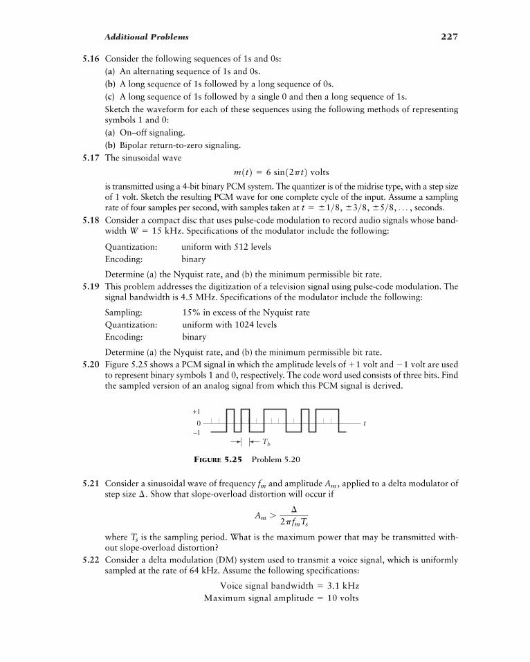
Additional Problems 227
5.16 Consider the following sequences of 1s and 0s:(a) An alternating sequence of 1s and 0s.(b) A long sequence of 1s followed by a long sequence of 0s.(c) A long sequence of 1s followed by a single 0 and then a long sequence of 1s.Sketch the waveform for each of these sequences using the following methods of representingsymbols 1 and 0:(a) On–off signaling.(b) Bipolar return-to-zero signaling.
5.17 The sinusoidal wave
is transmitted using a 4-bit binary PCM system. The quantizer is of the midrise type, with a step sizeof 1 volt. Sketch the resulting PCM wave for one complete cycle of the input. Assume a samplingrate of four samples per second, with samples taken at seconds.
5.18 Consider a compact disc that uses pulse-code modulation to record audio signals whose band-width Specifications of the modulator include the following:
Quantization: uniform with 512 levelsEncoding: binary
Determine (a) the Nyquist rate, and (b) the minimum permissible bit rate.5.19 This problem addresses the digitization of a television signal using pulse-code modulation. The
signal bandwidth is 4.5 MHz. Specifications of the modulator include the following:
Sampling: 15% in excess of the Nyquist rateQuantization: uniform with 1024 levelsEncoding: binary
Determine (a) the Nyquist rate, and (b) the minimum permissible bit rate.5.20 Figure 5.25 shows a PCM signal in which the amplitude levels of volt and volt are used
to represent binary symbols 1 and 0, respectively. The code word used consists of three bits. Findthe sampled version of an analog signal from which this PCM signal is derived.
�11
W � 15 kHz.
t � �1>8, �3>8, �5>8, Á ,
m1t2 � 6 sin12pt2 volts
t
Tb
0
+1
–1
FIGURE 5.25 Problem 5.20
5.21 Consider a sinusoidal wave of frequency and amplitude applied to a delta modulator ofstep size Show that slope-overload distortion will occur if
where is the sampling period. What is the maximum power that may be transmitted with-out slope-overload distortion?
5.22 Consider a delta modulation (DM) system used to transmit a voice signal, which is uniformlysampled at the rate of 64 kHz. Assume the following specifications:
Maximum signal amplitude � 10 voltsVoice signal bandwidth � 3.1 kHz
Ts
Am �¢
2pfmTs
¢ .Am ,fm
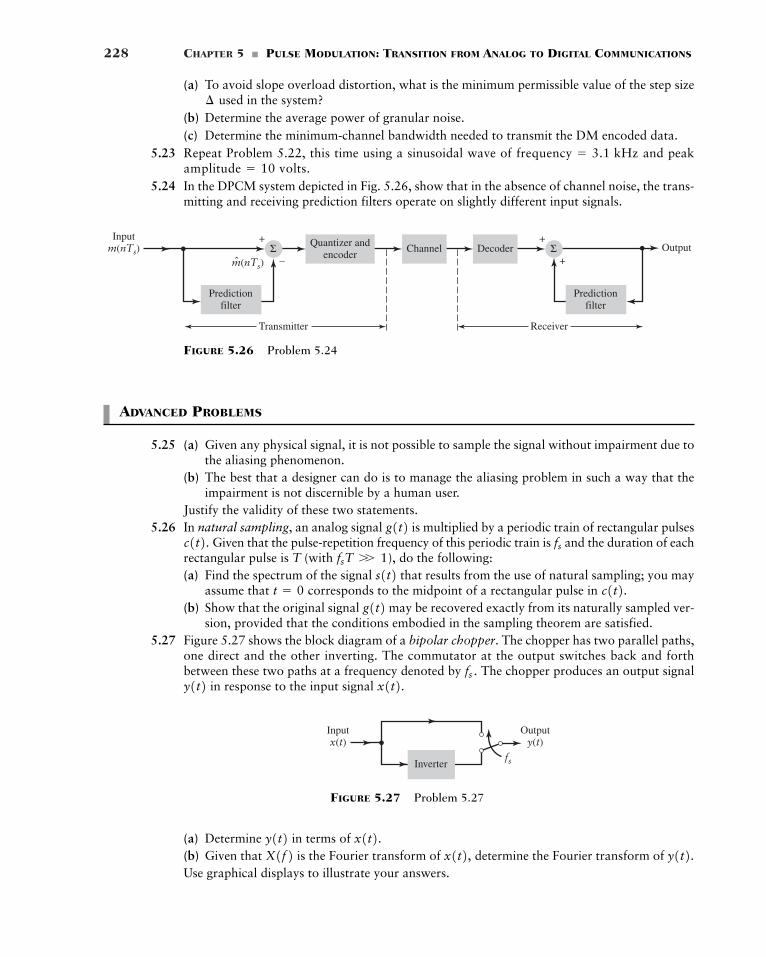
228 CHAPTER 5 � PULSE MODULATION: TRANSITION FROM ANALOG TO DIGITAL COMMUNICATIONS
(a) To avoid slope overload distortion, what is the minimum permissible value of the step sizeused in the system?
(b) Determine the average power of granular noise.(c) Determine the minimum-channel bandwidth needed to transmit the DM encoded data.
5.23 Repeat Problem 5.22, this time using a sinusoidal wave of and peak
5.24 In the DPCM system depicted in Fig. 5.26, show that in the absence of channel noise, the trans-mitting and receiving prediction filters operate on slightly different input signals.
amplitude � 10 volts.frequency � 3.1 kHz
¢
ADVANCED PROBLEMS
5.25 (a) Given any physical signal, it is not possible to sample the signal without impairment due tothe aliasing phenomenon.
(b) The best that a designer can do is to manage the aliasing problem in such a way that theimpairment is not discernible by a human user.
Justify the validity of these two statements.5.26 In natural sampling, an analog signal is multiplied by a periodic train of rectangular pulses
Given that the pulse-repetition frequency of this periodic train is and the duration of eachrectangular pulse is T (with ), do the following:(a) Find the spectrum of the signal that results from the use of natural sampling; you may
assume that corresponds to the midpoint of a rectangular pulse in (b) Show that the original signal may be recovered exactly from its naturally sampled ver-
sion, provided that the conditions embodied in the sampling theorem are satisfied.5.27 Figure 5.27 shows the block diagram of a bipolar chopper. The chopper has two parallel paths,
one direct and the other inverting. The commutator at the output switches back and forthbetween these two paths at a frequency denoted by The chopper produces an output signal
in response to the input signal x1t2.y1t2 fs .
g1t2 c1t2.t � 0s1t2fsT W 1
fsc1t2. g1t2
Receiver
Predictionfilter
Predictionfilter
Quantizer andencoder
Channel Decoder OutputInput
m(nTs)+
–Σ
+
+Σ
m(nTs)n
Transmitter
FIGURE 5.26 Problem 5.24
Inputx(t)
Outputy(t)
fsInverter
FIGURE 5.27 Problem 5.27
(a) Determine in terms of (b) Given that is the Fourier transform of determine the Fourier transform of Use graphical displays to illustrate your answers.
y1t2.x1t2,X1f2 x1t2.y1t2
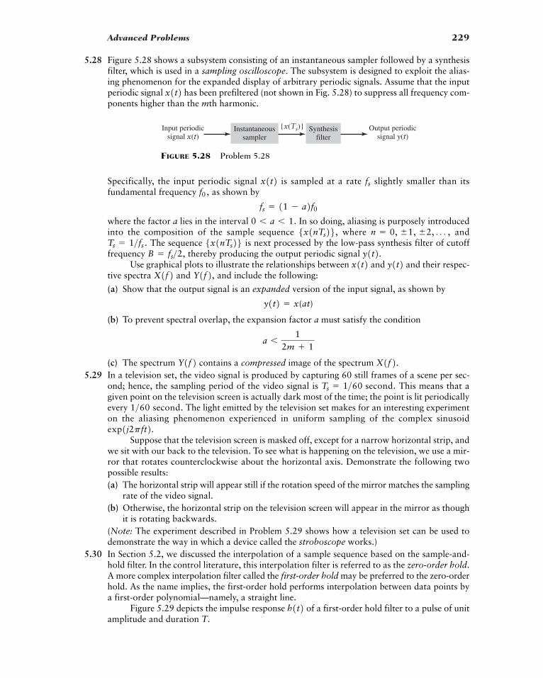
Advanced Problems 229
5.28 Figure 5.28 shows a subsystem consisting of an instantaneous sampler followed by a synthesisfilter, which is used in a sampling oscilloscope. The subsystem is designed to exploit the alias-ing phenomenon for the expanded display of arbitrary periodic signals. Assume that the inputperiodic signal has been prefiltered (not shown in Fig. 5.28) to suppress all frequency com-ponents higher than the mth harmonic.
x1t2
Specifically, the input periodic signal is sampled at a rate slightly smaller than itsfundamental frequency as shown by
where the factor a lies in the interval In so doing, aliasing is purposely introducedinto the composition of the sample sequence where and
The sequence is next processed by the low-pass synthesis filter of cutofffrequency thereby producing the output periodic signal
Use graphical plots to illustrate the relationships between and and their respec-tive spectra and and include the following:
(a) Show that the output signal is an expanded version of the input signal, as shown by
(b) To prevent spectral overlap, the expansion factor a must satisfy the condition
(c) The spectrum contains a compressed image of the spectrum 5.29 In a television set, the video signal is produced by capturing 60 still frames of a scene per sec-
ond; hence, the sampling period of the video signal is This means that agiven point on the television screen is actually dark most of the time; the point is lit periodicallyevery The light emitted by the television set makes for an interesting experimenton the aliasing phenomenon experienced in uniform sampling of the complex sinusoid
Suppose that the television screen is masked off, except for a narrow horizontal strip, andwe sit with our back to the television. To see what is happening on the television, we use a mir-ror that rotates counterclockwise about the horizontal axis. Demonstrate the following twopossible results:(a) The horizontal strip will appear still if the rotation speed of the mirror matches the sampling
rate of the video signal.(b) Otherwise, the horizontal strip on the television screen will appear in the mirror as though
it is rotating backwards.(Note: The experiment described in Problem 5.29 shows how a television set can be used todemonstrate the way in which a device called the stroboscope works.)
5.30 In Section 5.2, we discussed the interpolation of a sample sequence based on the sample-and-hold filter. In the control literature, this interpolation filter is referred to as the zero-order hold.A more complex interpolation filter called the first-order hold may be preferred to the zero-orderhold. As the name implies, the first-order hold performs interpolation between data points bya first-order polynomial—namely, a straight line.
Figure 5.29 depicts the impulse response of a first-order hold filter to a pulse of unitamplitude and duration T.
h1t2
exp1j2pft2.1>60 second.
Ts � 1>60 second.
X1f2.Y1f2a �
12m 1
y1t2 � x(at)
Y1f2,X1f2 y1t2x1t2y1t2.B � fs>2,5x1nTs26Ts � 1>fs .
n � 0, �1, �2, Á ,5x1nTs26,0 � a � 1.
fs � 11 � a2f0f0 ,
fsx1t2
Input periodicsignal x(t)
Output periodicsignal y(t)
{x(Ts)}Instantaneoussampler
Synthesisfilter
FIGURE 5.28 Problem 5.28
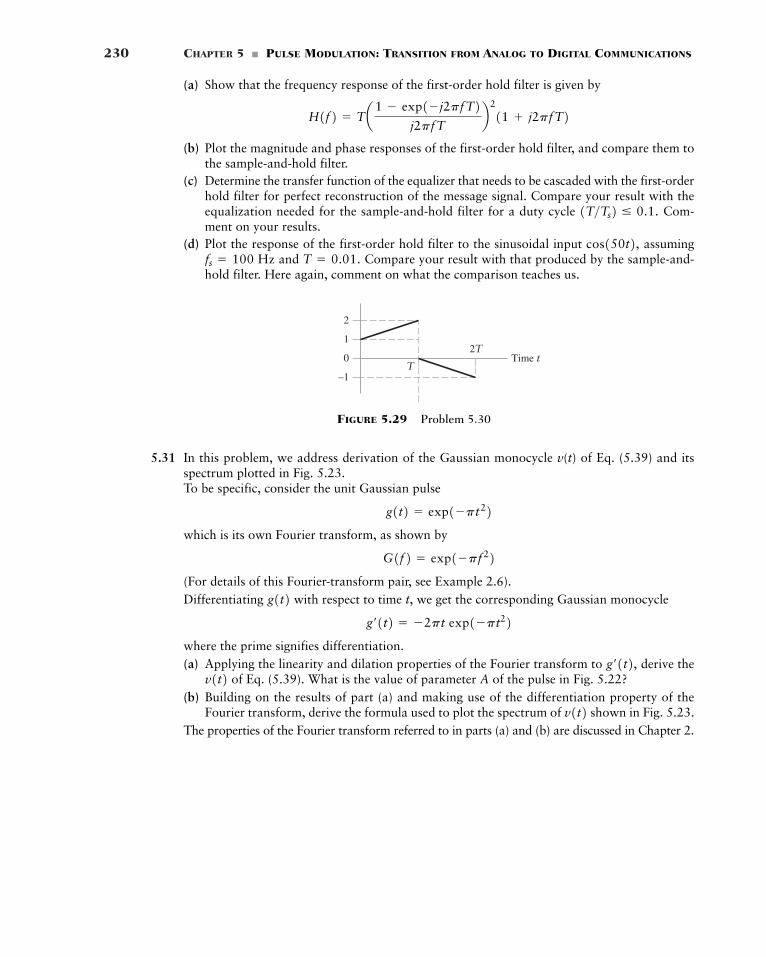
230 CHAPTER 5 � PULSE MODULATION: TRANSITION FROM ANALOG TO DIGITAL COMMUNICATIONS
(a) Show that the frequency response of the first-order hold filter is given by
(b) Plot the magnitude and phase responses of the first-order hold filter, and compare them tothe sample-and-hold filter.
(c) Determine the transfer function of the equalizer that needs to be cascaded with the first-orderhold filter for perfect reconstruction of the message signal. Compare your result with theequalization needed for the sample-and-hold filter for a duty cycle Com-ment on your results.
(d) Plot the response of the first-order hold filter to the sinusoidal input assumingand Compare your result with that produced by the sample-and-
hold filter. Here again, comment on what the comparison teaches us.T � 0.01.fs � 100 Hz
cos150t2,1T>Ts2 � 0.1.
H1f2 � Ta 1 � exp1�j2pfT2j2pfT
b 211 j2pfT2
2
1
0T
2TTime t
–1
FIGURE 5.29 Problem 5.30
5.31 In this problem, we address derivation of the Gaussian monocycle v(t) of Eq. (5.39) and itsspectrum plotted in Fig. 5.23.To be specific, consider the unit Gaussian pulse
which is its own Fourier transform, as shown by
(For details of this Fourier-transform pair, see Example 2.6).Differentiating with respect to time t, we get the corresponding Gaussian monocycle
where the prime signifies differentiation.(a) Applying the linearity and dilation properties of the Fourier transform to derive the
of Eq. (5.39). What is the value of parameter A of the pulse in Fig. 5.22?(b) Building on the results of part (a) and making use of the differentiation property of the
Fourier transform, derive the formula used to plot the spectrum of shown in Fig. 5.23.The properties of the Fourier transform referred to in parts (a) and (b) are discussed in Chapter 2.
v1t2v1t2 g�1t2,
g�1t2 � �2pt exp1�pt22g1t2
G1f2 � exp1�pf 22g1t2 � exp1�pt22
231
CHAPTER 6
BASEBAND DATA
TRANSMISSION
The transmission of digital data (regardless of their origin) over a physical communicationchannel is limited by two unavoidable factors:
1. Intersymbol interference, which arises due to imperfections in the frequency responseof the channel.
2. Channel noise, which refers to unwanted electric signals that arise at the channel out-put due to random and unpredictable physical phenomena.
In this chapter, we focus attention on the intersymbol interference problem. The discussionof noise in digital communication receivers is deferred to the latter part of the book.
As the name implies, intersymbol interference refers to interference caused by thetime response of the channel spilling over from one symbol into adjacent symbols. Inter-symbol interference is troublesome because it has the effect of introducing deviations (i.e.,errors) between the data sequence reconstructed at the receiver output and the originaldata sequence applied to the transmitter input. Hence, unless corrective measures aretaken, intersymbol interference could impose a limit on the attainable rate of data trans-mission across the channel, which is below the physical capability of the channel.
With intersymbol interference acting as an issue of practical concern, we will study animportant corrective measure to deal with it—namely, baseband pulse shaping. This mea-sure involves the use of band-limited pulses that are shaped in a special manner so as tomitigate the intersymbol interference problem; this corrective measure builds on priorknowledge about the channel.
The chapter will teach us three lessons:
� Lesson 1: Understanding of the intersymbol interference problem and how to cure it is offundamental importance to the design of digital communication systems.
� Lesson 2: The raised cosine spectrum provides a powerful mathematical tool for basebandpulse-shaping designed to mitigate the intersymbol interference problem.
� Lesson 3: The eye pattern is a visual indicator of performance, displaying the physical lim-itations of a digital data transmission system in an insightful manner.
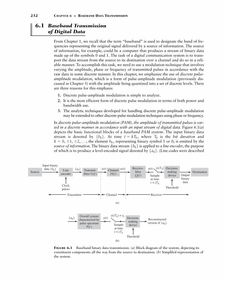
232 CHAPTER 6 � BASEBAND DATA TRANSMISSION
(a)
(b)
Overall systemcharacterized bypulse spectrum
P(f )
Decision-makingdeviceSample
at timet = iTb
{ak} y(t)y(iTb) = yi
Threshold
Reconstructedversion of {ak}
y(t)s(t) x(t) y(iTb)Source Line
encoderTransmit-filter G(f )
ChannelH(f )
DestinationReceive-
filterQ(f )
Decision-makingdevice Output
binarydata
Sampleat timet = iTb
Threshold
Input binarydata {bk} {ak}
Clockpulses
Transmitter Channel Receiver
FIGURE 6.1 Baseband binary data transmission. (a) Block diagram of the system, depicting itsconstituent components all the way from the source to destination. (b) Simplifed representation ofthe system.
6.1 Baseband Transmission of Digital Data
From Chapter 1, we recall that the term “baseband” is used to designate the band of fre-quencies representing the original signal delivered by a source of information. The sourceof information, for example, could be a computer that produces a stream of binary datamade up of the symbols 0 and 1. The task of a digital communication system is to trans-port the data stream from the source to its destination over a channel and do so in a reli-able manner. To accomplish this task, we need to use a modulation technique that involvesvarying the amplitude, phase or frequency of transmitted pulses in accordance with theraw data in some discrete manner. In this chapter, we emphasize the use of discrete pulse-amplitude modulation, which is a form of pulse-amplitude modulation (previously dis-cussed in Chapter 5) with the amplitude being quantized into a set of discrete levels. Thereare three reasons for this emphasis:
1. Discrete pulse-amplitude modulation is simple to analyze.2. It is the most efficient form of discrete pulse modulation in terms of both power and
bandwidth use.3. The analytic techniques developed for handling discrete pulse-amplitude modulation
may be extended to other discrete-pulse modulation techniques using phase or frequency.
In discrete pulse-amplitude modulation (PAM), the amplitude of transmitted pulses is var-ied in a discrete manner in accordance with an input stream of digital data. Figure 6.1(a)depicts the basic functional blocks of a baseband PAM system. The input binary datastream is denoted by At time where is the bit duration and
the element representing binary symbol 1 or 0, is emitted by thesource of information. The binary data stream is applied to a line encoder, the purposeof which is to produce a level-encoded signal denoted by (Line codes were described5ak6.5bk6bk ,k � 0, �1, �2, Á ;
Tbt � kTb ,5bk6.
6.2 The Intersymbol Interference Problem 233
in Chapter 5.) For example, we may define level-encoded signal in terms of positiveand negative pulses of fixed amplitude and short duration (short enough for the two pulsesto be viewed as unit impulses of opposite polarities). Specifically, we write
(6.1)
The level-encoded signal is applied to a transmit filter to produce a sequence of pulses,whose basic shape is denoted in the time and frequency domains by and respec-tively. In effect, the level-encoded signal plays the role of a modulating signal, withthe result that the discrete PAM signal is defined by
(6.2)
The PAM signal is transmitted across a linear communication channel, which isdescribed in the time and frequency domains by the impulse response and transferfunction respectively. Putting aside the effect of additive channel noise, we mayexpress the channel output as
(6.3)
where the symbol denotes convolution in the time domain.The channel output is processed by a receive-filter, which is described in the
time and frequency domains by the impulse response and transfer function respectively. The resulting output is therefore defined by the convolution of and —namely,
(6.4)
The filter output is next sampled synchronously with the generator of clock pulses inthe transmitter; synchronization is commonly established by extracting a clock or timingsignal from the receive-filter output. Finally, the sequence of samples thus obtained is usedto reconstruct the original binary data stream by means of a decision-making device. Specif-ically, the amplitude of each sample is compared to a threshold. If the threshold is exceeded,a decision is made in favor of symbol 1, say. If the threshold is not exceeded, a decision ismade in favor of symbol 0. If the sample amplitude equals the threshold exactly, the sym-bol may be chosen as 0 or 1 through the flip of a fair coin without affecting overall per-formance. For the case when symbols 0 and 1 are equiprobable, it is reasonable to set thethreshold at the zero amplitude level.
The model shown in Fig. 6.1(a) represents not only a data transmission system inher-ently baseband in nature (e.g., data transmission over a coaxial cable) but also the base-band equivalent of a linear modulation system used to transmit data over a band-passchannel (e.g., telephone channel). In the latter case, the baseband equivalent model of thedata transmission system is developed by using the ideas presented in Section 3.8.
6.2 The Intersymbol Interference Problem
As already mentioned, for the present discussion we ignore the effect of additive channelnoise. We do so in order to focus attention on the effects of imperfections in the frequencyresponse of the channel (i.e., dispersion of the pulse shape by the channel) on data trans-mission through the channel.
y1t2y1t2 � x1t2 � q1t2
q1t2x1t2 Q1f2,q1t2x1t2�
x1t2 � s1t2 � h1t2H1f2, h1t2s1t2
s1t2 � aq
k��qakg1t � kTb2
5ak6 G1f2,g1t25ak6ak � e1 if the input bk is symbol 1
�1 if the input bk is symbol 0
5ak6
234 CHAPTER 6 � BASEBAND DATA TRANSMISSION
1In practice, it may be preferable to sample the receive-filter output at times rather than The reason for doing so is the unavoidable presence of delay and distortion in the overall pulse response Tosimplify the presentation, we have ignored this effect.
p1t2.t � iTb .t � iTb t0y1t2
Using Eqs. (6.2) through (6.4), except for a scaling factor, we may express the receive-filter output as the modified PAM signal
(6.5)
Linearity of the data transmission depicted in Fig. 6.1 leads us to express the overall pulseshape in Eq. (6.5) by the multiple convolution product
(6.6)
Naturally, the received pulse has a shape different from that of the transmitted signalof Eq. (6.2). Let the spectrum denote the Fourier transform of the pulse
Then, in the frequency domain, we may equivalently write
(6.7)
As remarked previously, the receive-filter output of Eq. (6.5) is sampled synchronouslywith the transmitter. Let1
denote the sample of produced at time To simplify the presentation, we intro-duce the discrete-time shorthand notation:
and, correspondingly,
We thus rewrite the sample of at time compactly as the discrete convolution sum
(6.8)
Referring to Fig. 6.1(a), we see that is the input to the decision-making device.Define
(6.9)
where E is the transmitted signal energy per bit (symbol). The index i refers to the instantat which the receive-filter output is sampled in the receiver, whereas the index k refers toa symbol in the data stream produced by the source of information at the transmitted input.Thus, isolating the term representing in Eq. (6.8), we may equivalently write
(6.10)
In Eq. (6.10), the first term represents the transmitted binary symbol, except for the scal-ing factor The second term, involving the combined effect of all other transmitted2E .
ai
yi � 2Eai aq
k��qk i
akpi�k , i � 0, �1, �2, Á
k � i
p0 � p102 � 2E
yi � y1iTb2yi � a
q
k��qakpi�k , i � 0, �1, �2, Á
t � iTby1t2pi � p1iTb2yi � y1iTb2
t � iTb .y1t2y1iTb2 � a
q
k��qakp31i � k2Tb4, i � 0, �1, �2, Á
y1t2P1f2 � G1f2H1f2Q1f2
p1t2.P1f2s1t2 p1t2p1t2 � g1t2 � h1t2 � q1t2
p1t2
y1t2 � aq
k��qakp1t � kTb2
6.3 The Nyquist Channel 235
binary symbols before and after represents a residual phenomenon called the intersymbolinterference (ISI). In the absence of ISI (and the assumed absence of channel noise), Eq. (6.10)reduces to the ideal condition
which, of course, represents perfect decoding.The pulse-shaping problem involved in designing the PAM system of Fig. 6.1(a) may
now be stated as follows (ignoring the effect of channel noise):
Given the channel transfer function determine the transmit-pulse spectrumand receive-filter transfer function so as to satisfy two basic requirements:
(i) Intersymbol interference is reduced to zero.(ii) Transmission bandwidth is conserved.
To satisfy both of these requirements, we have to exercise control over the overall pulseshape in the time domain or, equivalently, the overall pulse spectrum in the fre-quency domain. The key question is how this control is actually exercised.
6.3 The Nyquist Channel
In light of Eqs. (6.5) and (6.7), we may replace the PAM system of Fig. 6.1(a) with thesimpler PAM configuration depicted in part (b) of the figure. The distinctive feature of Fig.6.1(b) is its focus on the overall pulse spectrum
For the optimum solution to the pulse-shaping problem, the condition for zero inter-symbol interference would have to be satisfied at the minimum transmission bandwidth pos-sible. With for all i defining the condition for zero intersymbol interference, weinfer from Eq. (6.10) that it is necessary for the overall pulse shape the inverse Fouriertransform of the pulse spectrum in Fig. 6.1(b), to satisfy the condition
(6.11)
Equation (6.11) implies sampling at a uniform rate equal to the bit rate Supposethat is band-limited to frequencies in the interval where is to bedefined. Then, invoking the interpolation formula of Eq. (5.7) that is embodied in the sam-pling theorem, we may express the pulse shape in terms of its sample values as
(6.12)
Suppose the bandwidth is related to the bit rate as
(6.13)
Then substituting Eq. (6.11) into Eq. (6.12), we obtain the sinc function
(6.14)
as the optimum pulse shape.
�2E sin12pB0t2
2pB0t
popt1t2 � 2E sinc12B0t2
B0 �1
2Tb
1>TbB0
p1t2 � aq
i��qp¢ i
2B0≤ sinc12B0t � i2p1t2
B0�B0 � f � B0,p1t2 1>Tb .p1t2pi � p1iTb2 � b2E , for i � 0
0, for all i 0
P1f2 p1t2,yi � ai
P1f2.
P1f2p1t2
Q1f2G1f2 H1f2,
yi � 2Eai , for all i
ai ,
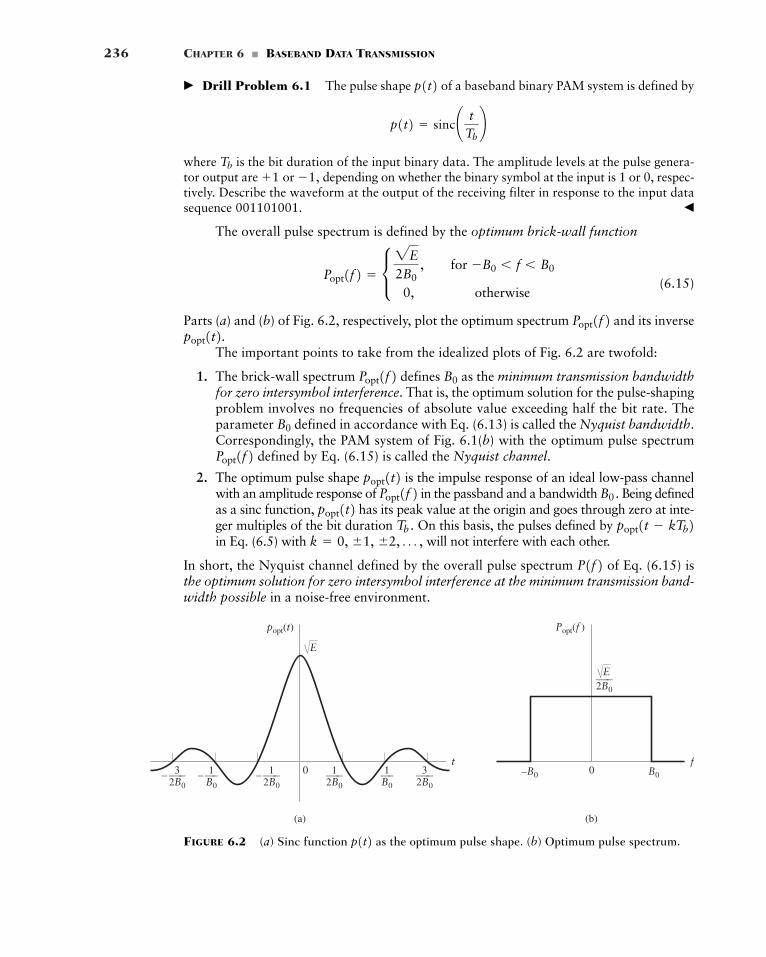
236 CHAPTER 6 � BASEBAND DATA TRANSMISSION
2B0
0
popt(t) Popt(f )
ft
(a)
0
(b)
—–– 32B0—–3
2B0—–
2B0—–– 1
2B0—–1
B0—–– 1
B0
B0–B0—–1
/E/E
FIGURE 6.2 (a) Sinc function as the optimum pulse shape. (b) Optimum pulse spectrum.p1t2
� Drill Problem 6.1 The pulse shape of a baseband binary PAM system is defined by
where is the bit duration of the input binary data. The amplitude levels at the pulse genera-tor output are or depending on whether the binary symbol at the input is 1 or 0, respec-tively. Describe the waveform at the output of the receiving filter in response to the input datasequence 001101001. �
The overall pulse spectrum is defined by the optimum brick-wall function
(6.15)
Parts (a) and (b) of Fig. 6.2, respectively, plot the optimum spectrum and its inverse
The important points to take from the idealized plots of Fig. 6.2 are twofold:
1. The brick-wall spectrum defines as the minimum transmission bandwidthfor zero intersymbol interference. That is, the optimum solution for the pulse-shapingproblem involves no frequencies of absolute value exceeding half the bit rate. Theparameter defined in accordance with Eq. (6.13) is called the Nyquist bandwidth.Correspondingly, the PAM system of Fig. 6.1(b) with the optimum pulse spectrum
defined by Eq. (6.15) is called the Nyquist channel.
2. The optimum pulse shape is the impulse response of an ideal low-pass channelwith an amplitude response of in the passband and a bandwidth Being definedas a sinc function, has its peak value at the origin and goes through zero at inte-ger multiples of the bit duration On this basis, the pulses defined by in Eq. (6.5) with will not interfere with each other.
In short, the Nyquist channel defined by the overall pulse spectrum of Eq. (6.15) isthe optimum solution for zero intersymbol interference at the minimum transmission band-width possible in a noise-free environment.
P1f2k � 0, �1, �2, Á ,
popt1t � kTb2Tb .popt1t2 B0.Popt1f 2popt1t2
Popt1f2B0
B0Popt1f2popt1t2. Popt1f2
Popt1f2 � c 2E2B0
, for �B0 � f � B0
0, otherwise
�1,1Tb
p1t2 � sinc¢ tTb≤p1t2
6.3 The Nyquist Channel 237
Although the Nyquist channel is indeed the optimum solution to the pulse-shapingproblem, there are two difficulties that make its use for a PAM system impractical:
1. The system requires that the spectrum be flat from to and zero else-where. This is physically unrealizable, and very difficult to approximate in practicebecause of the abrupt transitions at
2. The time function decreases as for large resulting in a slow rate of decay.This is caused by the discontinuity of at Accordingly, there is practicallyno margin of error in sampling times in the receiver.
To pursue the timing error problem under point 2, consider Eq. (6.5) and sample the at where is the timing error. To simplify the analysis, we shall put the correctsampling time equal to zero. We thus obtain (in the absence of channel noise)
Setting equal to the optimum value defined in the first line of Eq. (6.14) yields
With in accordance with Eq. (6.13), we may simplify the expression forinto
where, in the second line, we have done two things: isolate the term corresponding toand use the formula for the sinc function. Next, using the trigonometric identity
with and for all k, we may go one step further and write
(6.16)
The first term on the right-hand side of Eq. (6.16) defines the desired binary symbol,whereas the remaining series represents the intersymbol interference caused by the timingerror in sampling the signal The intersymbol interference so caused decays at therate Moreover, depending on the value of it is possible for this series to diverge,thereby causing erroneous decisions in the receiver.
To mitigate the problems due to physical realizability of the Nyquist channel andzero timing error, we therefore have to look to other pulse shapes. In the next section, wepresent one such solution that relaxes the minimum-bandwidth (ideal) solution embodiedin the Nyquist channel.
¢t,1>¢t.y1t2.¢t
y1¢t2 � 2Ea0 sinc12B0¢t2 2E¢ sin12pB0¢t2p
≤ aqk��q
k0
1�12kak
2B0¢t � k
sin1pk2 � 0cos1pk2 � 1�12ksin12pB0¢t � pk2 � sin12pB0¢t2 cos1pk2 � cos12pB0¢t2 sin1pk2
k � 0,
� 2Ea0 sinc12B0 ¢t2 2E aq
k��qk0
aksin12pB0¢t � pk2
2pB0¢t � pk
y1¢t2 � 2E aq
k��qak sinc12B0 ¢t � k2
y1¢t22B0Tb � 1
y1¢t2 � aq
k��qak sinc32B01¢t � kTb24
p1t2y1¢t2 � 2E a
q
k��qakp1¢t � kTb2, for iTb � 0
iTb
¢tt � ¢t,y1t2
�B0.P1f2 ƒt ƒ ,1> ƒt ƒp1t2 �B0.
B0,�B0P1f2
238 CHAPTER 6 � BASEBAND DATA TRANSMISSION
6.4 Raised-Cosine Pulse Spectrum
To ensure physical realizability of the overall pulse spectrum we need a solution thatdiffers from the Nyquist channel in one important respect: the modified decreasestoward zero gradually rather than abruptly. In more specific terms, is proposed to con-sist of two portions:
1. Flat portion, which occupies the frequency band for some parameter to be defined.
2. Roll-off portion, which occupies the frequency band
The parameter is adjustable under the designer’s control. The flat portion may thus retainpart of the ideal brick-wall solution. As for the roll-off portion, it provides for the gradualdecrease of toward zero. The key question is how to formulate this gradual roll-offcharacteristic. For the answer, we first look to one full cycle of the cosine function definedin the frequency domain, which is raised up by an amount equal to its amplitude. The nextthing we do is to split this function at the origin into two equal halves, separate them byan amount equal to the width of the flat portion under point 1, and finally use them toaccount for the roll-off portion under point 2. This new figure constitutes the desired shapefor the modified pulse spectrum For obvious reasons, the constructed in this man-ner is called the raised-cosine pulse spectrum.
To cast the raised-cosine pulse spectrum in mathematical terms, we write
(6.17)
The frequency and the Nyquist bandwidth are related by the new parameter
(6.18)
which is called the roll-off factor. For —that is, —we get the Nyquist chan-nel described in Section 6.3.
The spectrum normalized by multiplying it by is plotted in Fig. 6.3(a)versus the normalized frequency for three values of namely, 0, 0.5, and 1. We seethat for or 1, the function cuts off gradually as compared with the idealbrick-wall solution (corresponding to ).
The modified pulse shape —that is, the inverse Fourier transform of the raised-cosine pulse spectrum —is defined by
(6.19)
The time function of Eq. (6.19) consists of the product of two factors: the factorthat defines the Nyquist channel, and a second factor that decreases as
for large The first factor ensures zero crossings of at the desired samplinginstants of time with i an integer (positive and negative). The second factor reducesthe tails of the pulse considerably below the Nyquist channel, so that the transmission of
t � iTb
p1t2ƒt ƒ .1> ƒt ƒ22E sinc12B0t2
p1t2 � 2E sinc12B0t2¢ cos12paB0t21 � 16a2B0
2t2≤P1f2 p1t2 a � 0
P1f2a � 0.5a:f>B0
2B0>2E ,P1f2,f1 � B0a � 0
a � 1 �f1B0
B0f1
P1f2 � e 2E2B0
, 0 � ƒf ƒ � f1
2E4B0b1 cosBp1 ƒf ƒ � f12
21B0 � f12 R r , f1 � ƒf ƒ � 2B0 � f1
0, 2B0 � f1 � ƒf ƒ
P1f2P1f2.2f1
P1f2f1
f1 � ƒf ƒ � 2B0 � f1.
f10 � ƒf ƒ � f1
P1f2 P1f2P1f2,
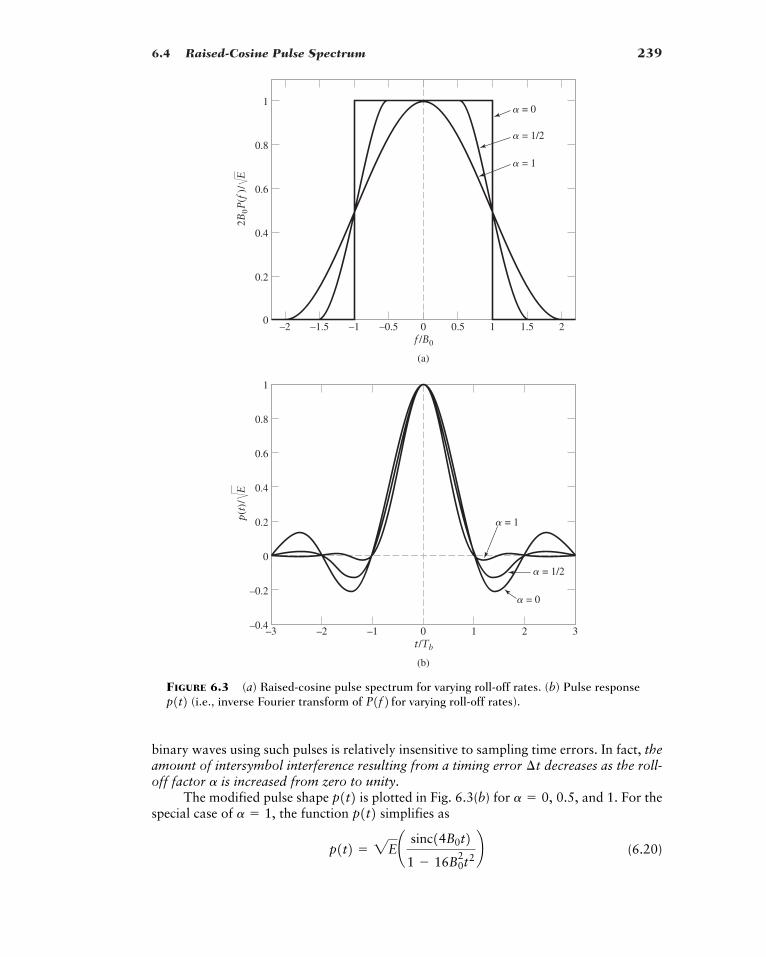
6.4 Raised-Cosine Pulse Spectrum 239
= 0
= 1/2
= 1
f /B0
–2 –1.5 –1 –0.5 0
(a)
0.5 1 1.5 2
0.2
0
2B0P
(f)//E
0.4
0.6
0.8
1
= 0
= 1/2
= 1
t/Tb
–2–3 –1 0 1 2 3
(b)
p(t)
//E
–0.2
0
0.2
0.4
0.6
0.8
1
–0.4
FIGURE 6.3 (a) Raised-cosine pulse spectrum for varying roll-off rates. (b) Pulse response(i.e., inverse Fourier transform of for varying roll-off rates).P1f2p1t2
binary waves using such pulses is relatively insensitive to sampling time errors. In fact, theamount of intersymbol interference resulting from a timing error decreases as the roll-off factor is increased from zero to unity.
The modified pulse shape is plotted in Fig. 6.3(b) for and 1. For thespecial case of the function simplifies as
(6.20)p1t2 � 2E¢ sinc14B0t21 � 16B0
2t2≤p1t2a � 1,
a � 0, 0.5,p1t2a
¢t
240 CHAPTER 6 � BASEBAND DATA TRANSMISSION
2For detailed discussion of this theorem, see Gitlin, Hayes and Weinstein (1992), p. 258.
The function of Eq. (6.20) exhibits two interesting properties:
1. At we have that is, the pulse width mea-sured at half amplitude is exactly equal to the bit duration
2. There are zero crossings at in addition to the usual zerocrossings at the sampling times
These two properties are particularly useful in the provision of a basis for extracting a tim-ing signal from the receive-filter output which is used to synchronize the receiver tothe transmitter.
� Drill Problem 6.2 Show that for positive frequencies, the area under the normalizedraised-cosine curve of versus is equal to unity for all values of the roll-off factor in the range A similar statement holds for negative frequencies. �
� Drill Problem 6.3 Given that is the Fourier transform of a pulse-like function we may state the following theorem:2
The pulse decreases asymptotically with time as provided that the followingtwo conditions hold:
1. The first derivatives of the Fourier transform with respect to frequency areall continuous.
2. The kth derivative of is discontinuous.
Demonstrate the validity of this theorem for the three different values of plotted in Fig. 6.3(a). �
� Drill Problem 6.4 Equation (6.17) defines the raised-cosine pulse spectrum as real-valued and therefore zero delay. In practice, every transmission system experiences some finitedelay. To accommodate this practicality, we may associate with a linear phase character-istic over the frequency band
(a) Show that this modification of introduces a finite delay into its inverse Fourier trans-form, namely, the pulse shape
(b) According to Eq. (6.19), represents a non-causal time response. The delay intro-duced into through the modification of has also a beneficial effect, tending tomake essentially causal. For this to happen, however, the delay must not be less thana certain value dependent on the roll-off factor Suggest suitable values for the delay for
and 1. �
� TRANSMISSION-BANDWIDTH REQUIREMENT
From Eq. (6.17) we see that the nonzero portion of the raised-cosine pulse spectrum is limited to the interval for positive frequencies. Accordingly, the transmis-sion bandwidth required by using the raised-cosine pulse spectrum is given by
Eliminating between Eq. (6.18) and this formula for we obtain
(6.21)
where is the Nyquist bandwidth and is the roll-off factor. Thus, the transmissionbandwidth requirement of the raised-cosine spectrum exceeds that of the optimum Nyquistchannel by the amount
(6.22)fn � aB0
aB0
BT � B011 a2BT ,f1
BT � 2B0 � f1
10, 2B0 � f12 P1f2
a � 0, 1>2,a.
p1t2 P1f2p1t2 p1t2p1t2.P1f20 � ƒ f ƒ � 2B0 � f1 .
P1f2P1f2a
P1f2fP1f2k � 1
1>tk1p1t2p1t2,P1f2
0 � a � 1.f>B0P1f2> A2E>2B0 B
y1t2,t � �Tb , �2Tb , Á .
t � �3Tb>2, �5Tb>2, Á ,Tb .
p1t2 � 0.52E;t � �Tb>2 � �1>(4B0) ,
p1t2
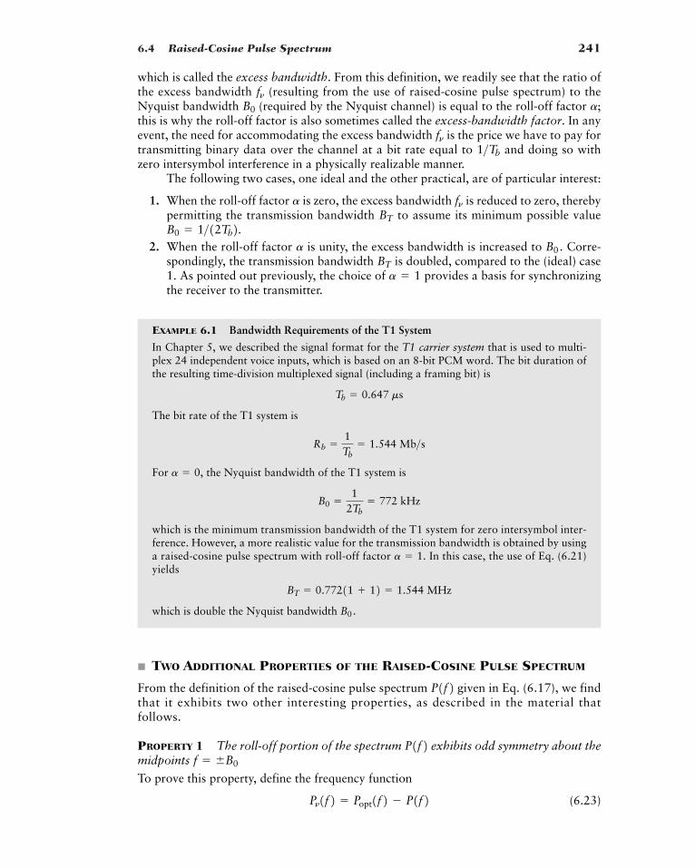
6.4 Raised-Cosine Pulse Spectrum 241
which is called the excess bandwidth. From this definition, we readily see that the ratio ofthe excess bandwidth (resulting from the use of raised-cosine pulse spectrum) to theNyquist bandwidth (required by the Nyquist channel) is equal to the roll-off factor this is why the roll-off factor is also sometimes called the excess-bandwidth factor. In anyevent, the need for accommodating the excess bandwidth is the price we have to pay fortransmitting binary data over the channel at a bit rate equal to and doing so withzero intersymbol interference in a physically realizable manner.
The following two cases, one ideal and the other practical, are of particular interest:
1. When the roll-off factor is zero, the excess bandwidth is reduced to zero, therebypermitting the transmission bandwidth to assume its minimum possible value
2. When the roll-off factor is unity, the excess bandwidth is increased to Corre-spondingly, the transmission bandwidth is doubled, compared to the (ideal) case1. As pointed out previously, the choice of provides a basis for synchronizingthe receiver to the transmitter.
EXAMPLE 6.1 Bandwidth Requirements of the T1 System
In Chapter 5, we described the signal format for the T1 carrier system that is used to multi-plex 24 independent voice inputs, which is based on an 8-bit PCM word. The bit duration ofthe resulting time-division multiplexed signal (including a framing bit) is
The bit rate of the T1 system is
For the Nyquist bandwidth of the T1 system is
which is the minimum transmission bandwidth of the T1 system for zero intersymbol inter-ference. However, a more realistic value for the transmission bandwidth is obtained by usinga raised-cosine pulse spectrum with roll-off factor In this case, the use of Eq. (6.21)yields
which is double the Nyquist bandwidth
� TWO ADDITIONAL PROPERTIES OF THE RAISED-COSINE PULSE SPECTRUM
From the definition of the raised-cosine pulse spectrum given in Eq. (6.17), we findthat it exhibits two other interesting properties, as described in the material thatfollows.
PROPERTY 1 The roll-off portion of the spectrum exhibits odd symmetry about themidpoints
To prove this property, define the frequency function
(6.23)Pn1f2 � Popt1f2 � P1f2f � �B0
P1f2
P1f2
B0.
BT � 0.77211 12 � 1.544 MHz
a � 1.
B0 �1
2Tb� 772 kHz
a � 0,
Rb �1Tb
� 1.544 Mb>s
Tb � 0.647 ms
a � 1BT
B0.a
B0 � 1>12Tb2. BT
fna
1>Tb
fn
a;B0
fn
242 CHAPTER 6 � BASEBAND DATA TRANSMISSION
(a)
0Frequency f
Raised cosine spectrum, P(f )
Pulsespectrum
Nyquist spectrum, Popt(f )
B0 B0 + fv
Excessbandwidth
fv
2B0—––/E
4B0—––/E
(b)
0 Frequency f
ResidualspectrumPv(f )
B0 B0 + fvB0 – fv
4B0—–––/E
4B0—––/E
which is a unique characterization of the roll-off portion of the raised-cosine spectrum.Using Eqs. (6.15) and (6.17) in this definition yields
(6.24)
Figure 6.4(a) plots and for roll-off factor only plots for positive fre-quencies are shown in the figure. The corresponding residual function is plotted inFig. 6.4(b). From this figure we immediately see that
(6.25)
where
(6.26)
Equation (6.25) confirms the odd-property of the roll-off portion about the midpointfor positive frequencies. Similarly, this property also holds at the other midpoint
for negative frequencies.f � �B0
f � B0
f� � f � B0
Pn1�f�2 � �Pn1f�2Pn1f2a � 1>2;P1f2Popt1f2
Pn1f2 � g 0, for 0 � ƒf ƒ � f12E
4B0b1 � cosBp1 ƒf ƒ � f12
21B0 � f12R r , for f1 � ƒf ƒ � B0
�2E4B0
b1 cosBp1 ƒf ƒ � f1221B0 � f12R r , for B0 � ƒf ƒ � 2B0 � f1
0, for 2B0 � f1 � ƒf ƒ � 2B0
FIGURE 6.4 (a) Nyquist and raised-cosine pulse spectra for positive frequencies. (b) Residual spectrum Pn1f2.
6.4 Raised-Cosine Pulse Spectrum 243
� Drill Problem 6.5 Starting with the formula of Eq. (6.24) and using the definition ofEq. (6.26), demonstrate the property of Eq. (6.25). �
The spectral characteristic portrayed in Fig. 6.4(a) reminds us of a similar situationpertaining to vestigial sideband modulation, which was studied in Chapter 3. Specifically,comparing Figs. 3.24(a) and 6.4(a), we readily see that although these two spectral char-acteristics refer to entirely different applications, they are basically of an identical mathe-matical form, except for two minor differences:
1. The baseband raised-cosine pulse spectrum of Fig. 6.4(a) is centered on the ori-gin at whereas the vestigial sideband spectrum of Fig. 3.24(a) is centered onthe sinusoidal carrier frequency
2. The parameter in Fig. 6.4(a) refers to the excess bandwidth measured with respectto the ideal brick-wall solution for zero intersymbol interference, whereas the para-meter in Fig. 3.24(a) refers to the excess bandwidth measured with respect to theoptimum bandwidth attainable with single sideband modulation.
Difference 1 is of a technical nature, and difference 2 merely pertains to terminology. Whatis really important to note is that in both applications, where the raised-cosine pulse spec-trum is intended for baseband digital data transmission and the vestigial sideband spectrumis usually (but not always) intended for analog modulation, the motivation is to ensurephysical realizability.3 (The Theme Example on digital television to be presented in Chap-ter 7 uses vestigial sideband modulation.)
PROPERTY 2 The infinite summation of replicas of the raised-cosine pulse spectrum,spaced by hertz, equals a constant, as shown by
(6.27)
To prove this property, recall from Chapter 2 that sampling of a Fourier transformablefunction in the time domain is transformed into periodicity in the frequency domain, asdescribed in Eq. (2.88). Adapting this equation to the situation at hand, we may write
(6.28)
The raised-cosine pulse spectrum and its inverse are respectively defined in Eqs.(6.17) and (6.19). In particular, sampling the modified pulse response at the rate
we may write
p¢ n2B0≤ � 2E sinc1n2¢ cos1pna2
1 � 4n2a2 ≤1>2B0,p1t2p1t2P1f2
aq
n��qp¢ n
2B0≤d¢t �
n2B0≤ Δ 2B0 a
q
m��qP1f � 2mB02
aq
m��qP1f � 2mB02 �
2E2B0
2B0
fv
fv
fc .f � 0,
P1f2
3It is even more interesting to note, that Harry Nyquist is the originator of both vestigial sideband modulationand raised-cosine pulse spectrum:
The spectral shaping for vestigial sideband modulation appeared in the paper, H. Nyquist and K. W. Pfleger,“Effect of the quadrature component in single-sideband transmission,” The Bell System Technical Journal, vol.19, pp. 63–73, January 1940.
The raised-cosine pulse spectrum was described in the earlier classic paper: H. Nyquist, “Certain topicsin telegraph transmission theory”, Transactions of the American Institute of Electrical Engineers, vol. 47,pp. 617–644, April 1928.
244 CHAPTER 6 � BASEBAND DATA TRANSMISSION
where Noting the two points:
1.
2.
it follows that
Accordingly, Eq. (6.28) reduces to
or, equivalently,
(6.29)
Finally, noting that the Fourier transform of the delta function is unity, Eq. (6.29) ismerely another way of describing the desired form shown in Eq. (6.27).
Having proved the validity of Property 2, we may turn it around. Specifically, thepulse-shaping criterion for zero intersymbol interference is embodied in the following gen-eral statement:
Given the modified pulse shape for transmitting data over an imperfect channel usingdiscrete pulse-amplitude modulation at the data rate the pulse shape elimi-nates intersymbol interference if, and only if, its spectrum satisfies the condition
(6.30)
This statement includes binary PAM as a special case, for which the data rate equalsin accordance with Eq. (6.13). Moreover, the raised-cosine pulse spectrum is one exam-
ple, albeit an important one, that satisfies Eq. (6.30).
� ROOT RAISED-COSINE PULSE SPECTRUM
A more sophisticated form of pulse shaping for baseband digital data transmission is to usethe root raised-cosine pulse spectrum rather than the regular pulse-shaping spectrum ofEq. (6.17). Specifically, we write
(6.31)
where, as before, is the transmit-filter’s frequency response and is the channel’sfrequency response. Correspondingly, the receive-filter’s frequency response is defined by
(6.32)
Multiplying Eq. (6.31) by (6.32) yields
G1f2H1f2Q1f2 � P1f2Q1f2 � P1>21f2
H1f2G1f2G1f2H1f2 � P1>21f2
2B0
1>Tb
aq
m� �qPa f �
mTb � constant, ƒ f ƒ �
12T
P1f2 p1t21>T,p1t2
d1t22E2B0d1t2 Δ a
q
m��qP1f � 2mB02
2Ed1t2 Δ 2B0 aq
m��qP1f � 2mB02
p¢ n2B0≤ � b2E , for n � 0
0, for n � �1, �2, Á
cos1pna2 � 1 for n � 0,
� b1, for n � 00, for n � �1, �2, Á
sinc1n2 �sin1np2
np
n � 0, �1, �2, Á .
6.5 Baseband Transmission of M-Ary Data 245
which is a repeat of Eq. (6.7). On this basis, the pulse shaping is partitioned equally betweentwo entities:
� The combination of transmit-filter and channel constitutes one entity. With known and defined by Eq. (6.17) for a prescribed roll-off factor we may useEq. (6.31) to determine the frequency response of the transmit filter.
� The receive filter constitutes the other entity. Hence, for the same roll-off factor wemay use Eqs. (6.17) and (6.32) to determine the frequency response of the receive-filter.
If the channel is affected by additive noise and the pulse-shaping is partitioned equallybetween the transmitter and receiver in the manner described herein, then the receiverwould maximize the output signal-to-noise ratio at the sampling instants. Further discus-sion of this issue is deferred to Chapter 10, which is devoted to noise in digital communi-cation receivers.
6.5 Baseband Transmission of M-ary Data
In the baseband binary PAM system of Fig. 6.1(a), the sequence emitted by the sourceof information consists of binary symbols that are represented by one of two possibleamplitude levels, for symbol 0 and for symbol 1. On the other hand, in a basebandM-ary version of the system, the output of the line encoder takes on one of M possible ampli-tude levels with In an M-ary system, the information source emits a sequence ofsymbols from an alphabet that consists of M symbols. Each amplitude level at the line-encoder output corresponds to a distinct symbol, so that there are M distinct amplitude lev-els to be transmitted.
Consider then an M-ary PAM system with a signal alphabet that contains M symbols,with the symbol duration denoted by T seconds. We refer to as the signaling rate orsymbol rate of the system, which is expressed in symbols per second or simply bauds. It isinformative to relate the signaling rate of this system to that of an equivalent binary PAMsystem for which the value of M is 2 and the bit duration is seconds. The binary PAMsystem transmits data at the rate of bits per second. We also observe that in the caseof a quaternary PAM system, for example, the four possible symbols may be identifiedwith the dibits 00, 10, 11, and 01; a dibit refers to a word consisting of two bits. We thussee that each symbol represents 2 bits of data and 1 baud is equal to 2 bits per second. Wemay generalize this result by stating that in an M-ary PAM system, 1 baud is equal to
bits per second, and the symbol duration T of the M-ary PAM system is related tothe bit duration of a binary PAM system with the equivalent bit rate as follows:
(6.33)
Therefore, in a given channel bandwidth, we find that by using an M-ary PAM system weare able to transmit data at a rate that is faster than the corresponding binary PAMsystem.
However, this improvement in bandwidth utilization is attained at a price. Specifically,the transmitted power must be increased by a factor equal to compared to abinary PAM system, if we are to realize the same performance in the presence of channelnoise; this issue is discussed in Chapter 10. Also, system complexity is increased.
M2>log2 M,
log2 M
T � Tb log2 M
Tb
log2 M
1>Tb
Tb
1>T
M � 2.
1�1
5bk6
a
a,P1f2 H1f2
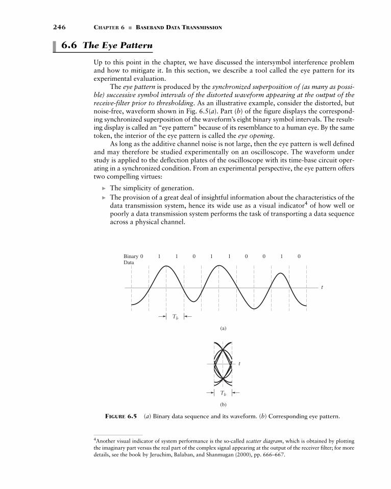
246 CHAPTER 6 � BASEBAND DATA TRANSMISSION
4Another visual indicator of system performance is the so-called scatter diagram, which is obtained by plottingthe imaginary part versus the real part of the complex signal appearing at the output of the receiver filter; for moredetails, see the book by Jeruchim, Balaban, and Shanmugan (2000), pp. 666–667.
6.6 The Eye Pattern
Up to this point in the chapter, we have discussed the intersymbol interference problemand how to mitigate it. In this section, we describe a tool called the eye pattern for itsexperimental evaluation.
The eye pattern is produced by the synchronized superposition of (as many as possi-ble) successive symbol intervals of the distorted waveform appearing at the output of thereceive-filter prior to thresholding. As an illustrative example, consider the distorted, butnoise-free, waveform shown in Fig. 6.5(a). Part (b) of the figure displays the correspond-ing synchronized superposition of the waveform’s eight binary symbol intervals. The result-ing display is called an “eye pattern” because of its resemblance to a human eye. By the sametoken, the interior of the eye pattern is called the eye opening.
As long as the additive channel noise is not large, then the eye pattern is well definedand may therefore be studied experimentally on an oscilloscope. The waveform understudy is applied to the deflection plates of the oscilloscope with its time-base circuit oper-ating in a synchronized condition. From an experimental perspective, the eye pattern offerstwo compelling virtues:
� The simplicity of generation.� The provision of a great deal of insightful information about the characteristics of the
data transmission system, hence its wide use as a visual indicator4 of how well orpoorly a data transmission system performs the task of transporting a data sequenceacross a physical channel.
(a)
(b)
BinaryData
0 1 1
Tb
0 0 0 01 1 1
t
Tb
t
FIGURE 6.5 (a) Binary data sequence and its waveform. (b) Corresponding eye pattern.
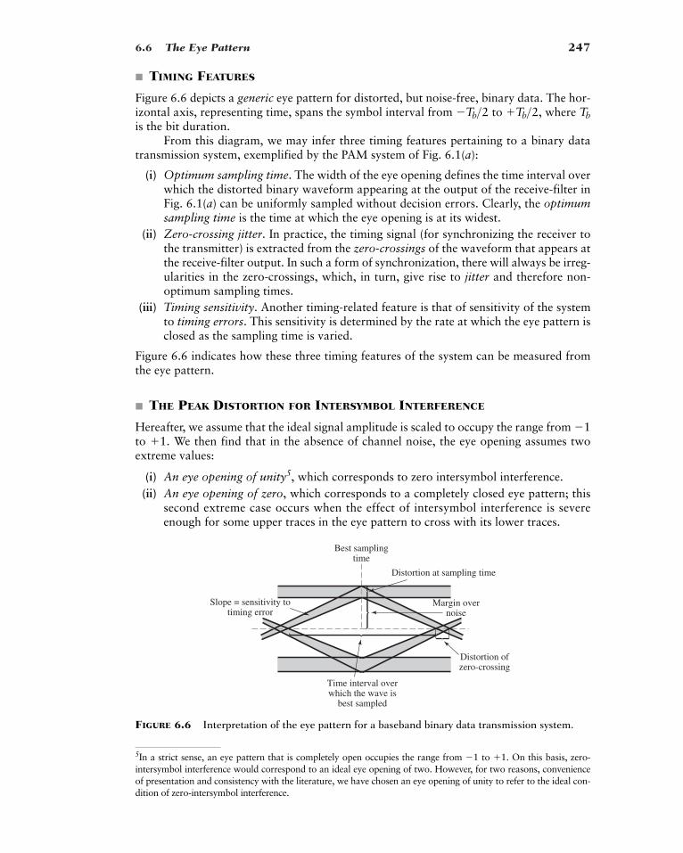
6.6 The Eye Pattern 247
Best samplingtime
Time interval overwhich the wave is
best sampled
Distortion at sampling time
Margin overnoise
Distortion ofzero-crossing
Slope = sensitivity totiming error
� TIMING FEATURES
Figure 6.6 depicts a generic eye pattern for distorted, but noise-free, binary data. The hor-izontal axis, representing time, spans the symbol interval from to where is the bit duration.
From this diagram, we may infer three timing features pertaining to a binary datatransmission system, exemplified by the PAM system of Fig. 6.1(a):
(i) Optimum sampling time. The width of the eye opening defines the time interval overwhich the distorted binary waveform appearing at the output of the receive-filter inFig. 6.1(a) can be uniformly sampled without decision errors. Clearly, the optimumsampling time is the time at which the eye opening is at its widest.
(ii) Zero-crossing jitter. In practice, the timing signal (for synchronizing the receiver tothe transmitter) is extracted from the zero-crossings of the waveform that appears atthe receive-filter output. In such a form of synchronization, there will always be irreg-ularities in the zero-crossings, which, in turn, give rise to jitter and therefore non-optimum sampling times.
(iii) Timing sensitivity. Another timing-related feature is that of sensitivity of the systemto timing errors. This sensitivity is determined by the rate at which the eye pattern isclosed as the sampling time is varied.
Figure 6.6 indicates how these three timing features of the system can be measured fromthe eye pattern.
� THE PEAK DISTORTION FOR INTERSYMBOL INTERFERENCE
Hereafter, we assume that the ideal signal amplitude is scaled to occupy the range from to We then find that in the absence of channel noise, the eye opening assumes twoextreme values:
(i) An eye opening of unity5, which corresponds to zero intersymbol interference.(ii) An eye opening of zero, which corresponds to a completely closed eye pattern; this
second extreme case occurs when the effect of intersymbol interference is severeenough for some upper traces in the eye pattern to cross with its lower traces.
1.�1
TbTb>2,�Tb>2
5In a strict sense, an eye pattern that is completely open occupies the range from to . On this basis, zero-intersymbol interference would correspond to an ideal eye opening of two. However, for two reasons, convenienceof presentation and consistency with the literature, we have chosen an eye opening of unity to refer to the ideal con-dition of zero-intersymbol interference.
1�1
FIGURE 6.6 Interpretation of the eye pattern for a baseband binary data transmission system.
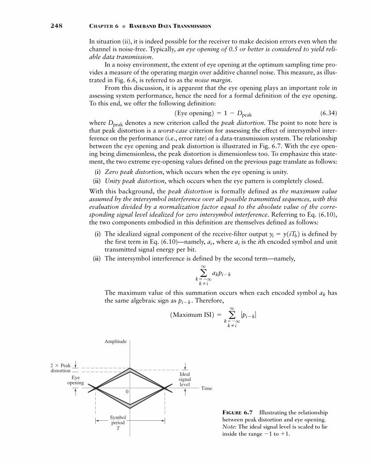
248 CHAPTER 6 � BASEBAND DATA TRANSMISSION
In situation (ii), it is indeed possible for the receiver to make decision errors even when thechannel is noise-free. Typically, an eye opening of 0.5 or better is considered to yield reli-able data transmission.
In a noisy environment, the extent of eye opening at the optimum sampling time pro-vides a measure of the operating margin over additive channel noise. This measure, as illus-trated in Fig. 6.6, is referred to as the noise margin.
From this discussion, it is apparent that the eye opening plays an important role inassessing system performance, hence the need for a formal definition of the eye opening.To this end, we offer the following definition:
(6.34)
where denotes a new criterion called the peak distortion. The point to note here isthat peak distortion is a worst-case criterion for assessing the effect of intersymbol inter-ference on the performance (i.e., error rate) of a data-transmission system. The relationshipbetween the eye opening and peak distortion is illustrated in Fig. 6.7. With the eye open-ing being dimensionless, the peak distortion is dimensionless too. To emphasize this state-ment, the two extreme eye-opening values defined on the previous page translate as follows:
(i) Zero peak distortion, which occurs when the eye opening is unity.(ii) Unity peak distortion, which occurs when the eye pattern is completely closed.
With this background, the peak distortion is formally defined as the maximum valueassumed by the intersymbol interference over all possible transmitted sequences, with thisevaluation divided by a normalization factor equal to the absolute value of the corre-sponding signal level idealized for zero intersymbol interference. Referring to Eq. (6.10),the two components embodied in this definition are themselves defined as follows:
(i) The idealized signal component of the receive-filter output is defined bythe first term in Eq. (6.10)—namely, where is the ith encoded symbol and unittransmitted signal energy per bit.
(ii) The intersymbol interference is defined by the second term—namely,
The maximum value of this summation occurs when each encoded symbol hasthe same algebraic sign as Therefore,
1Maximum ISI2 � aq
k��qk i
ƒpi�k ƒ
pi�k .ak
aq
k��qk i
akpi�k
aiai ,yi � y1iTb2
Dpeak
1Eye opening2 � 1 � Dpeak
Amplitude
Time
2*Peakdistortion
Eyeopening
Idealsignallevel
Symbolperiod
T
0
FIGURE 6.7 Illustrating the relationshipbetween peak distortion and eye opening.Note: The ideal signal level is scaled to lieinside the range to 1.�1
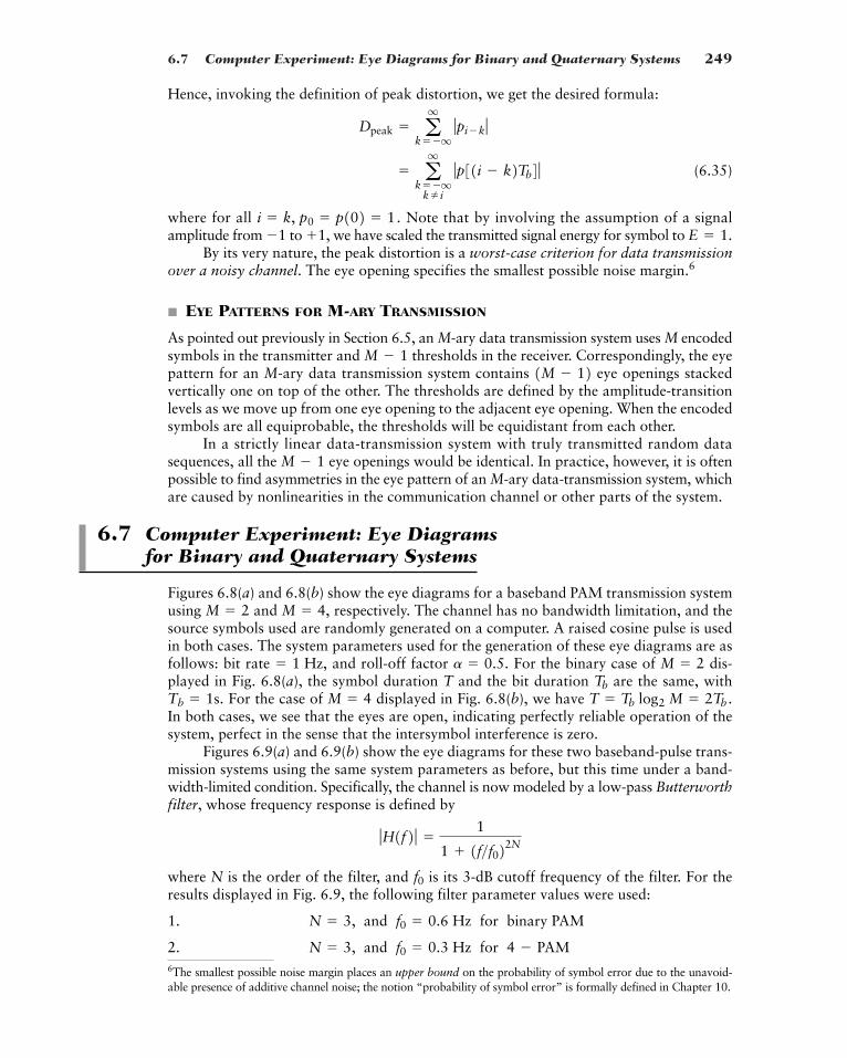
6.7 Computer Experiment: Eye Diagrams for Binary and Quaternary Systems 249
6The smallest possible noise margin places an upper bound on the probability of symbol error due to the unavoid-able presence of additive channel noise; the notion “probability of symbol error” is formally defined in Chapter 10.
Hence, invoking the definition of peak distortion, we get the desired formula:
(6.35)
where for all Note that by involving the assumption of a signalamplitude from to , we have scaled the transmitted signal energy for symbol to
By its very nature, the peak distortion is a worst-case criterion for data transmissionover a noisy channel. The eye opening specifies the smallest possible noise margin.6
� EYE PATTERNS FOR M-ARY TRANSMISSION
As pointed out previously in Section 6.5, an M-ary data transmission system uses M encodedsymbols in the transmitter and thresholds in the receiver. Correspondingly, the eyepattern for an M-ary data transmission system contains eye openings stackedvertically one on top of the other. The thresholds are defined by the amplitude-transitionlevels as we move up from one eye opening to the adjacent eye opening. When the encodedsymbols are all equiprobable, the thresholds will be equidistant from each other.
In a strictly linear data-transmission system with truly transmitted random datasequences, all the eye openings would be identical. In practice, however, it is oftenpossible to find asymmetries in the eye pattern of an M-ary data-transmission system, whichare caused by nonlinearities in the communication channel or other parts of the system.
6.7 Computer Experiment: Eye Diagramsfor Binary and Quaternary Systems
Figures 6.8(a) and 6.8(b) show the eye diagrams for a baseband PAM transmission systemusing and respectively. The channel has no bandwidth limitation, and thesource symbols used are randomly generated on a computer. A raised cosine pulse is usedin both cases. The system parameters used for the generation of these eye diagrams are asfollows: bit rate and roll-off factor For the binary case of dis-played in Fig. 6.8(a), the symbol duration T and the bit duration are the same, with
For the case of displayed in Fig. 6.8(b), we have In both cases, we see that the eyes are open, indicating perfectly reliable operation of thesystem, perfect in the sense that the intersymbol interference is zero.
Figures 6.9(a) and 6.9(b) show the eye diagrams for these two baseband-pulse trans-mission systems using the same system parameters as before, but this time under a band-width-limited condition. Specifically, the channel is now modeled by a low-pass Butterworthfilter, whose frequency response is defined by
where N is the order of the filter, and is its 3-dB cutoff frequency of the filter. For theresults displayed in Fig. 6.9, the following filter parameter values were used:
1. , and for binary PAM
2. , and for PAM4 �f0 � 0.3 HzN � 3
f0 � 0.6 HzN � 3
f0
ƒH1f2 ƒ �1
1 1f>f022N
T � Tb log2 M � 2Tb .M � 4Tb � 1s.Tb
M � 2a � 0.5.� 1 Hz,
M � 4,M � 2
M � 1
1M � 12M � 1
E � 1.1�1i � k, p0 � p102 � 1.
� aq
k��qk i
ƒp31i � k2Tb4 ƒDpeak � a
q
k��qƒpi�k ƒ
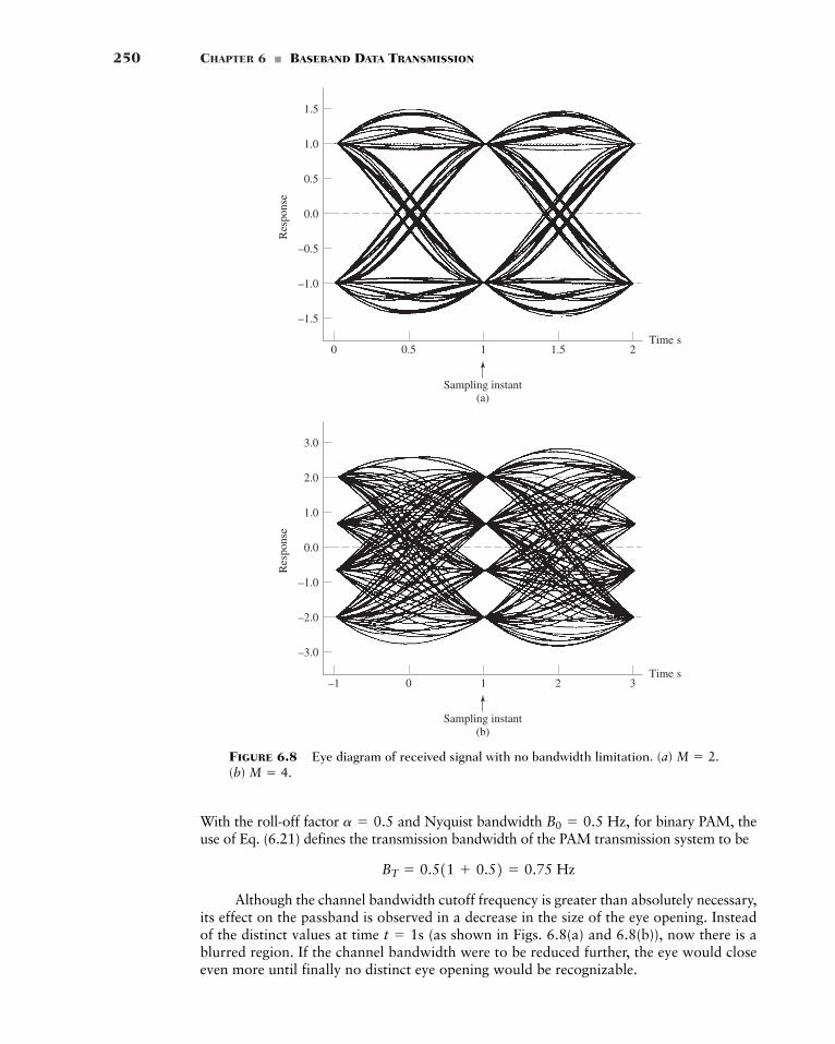
250 CHAPTER 6 � BASEBAND DATA TRANSMISSION
0 0.5 1 1.5 2
Res
pons
e
–1.5
–1.0
–0.5
0.0
0.5
1.0
1.5
Sampling instant(a)
Time s
Time s–1 0 1 2 3
Res
pons
e
–3.0
–2.0
–1.0
0.0
1.0
2.0
3.0
Sampling instant(b)
FIGURE 6.8 Eye diagram of received signal with no bandwidth limitation. (a)(b) M � 4.
M � 2.
With the roll-off factor and Nyquist bandwidth for binary PAM, theuse of Eq. (6.21) defines the transmission bandwidth of the PAM transmission system to be
Although the channel bandwidth cutoff frequency is greater than absolutely necessary,its effect on the passband is observed in a decrease in the size of the eye opening. Insteadof the distinct values at time (as shown in Figs. 6.8(a) and 6.8(b)), now there is ablurred region. If the channel bandwidth were to be reduced further, the eye would closeeven more until finally no distinct eye opening would be recognizable.
t � 1s
BT � 0.511 0.52 � 0.75 Hz
B0 � 0.5 Hz,a � 0.5
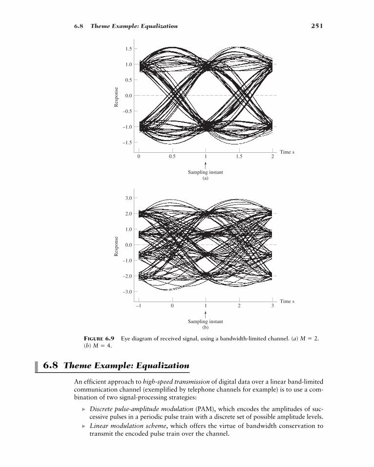
6.8 Theme Example: Equalization 251
0 0.5 1 1.5 2
Res
pons
e
–1.5
–1.0
–0.5
0.0
0.5
1.0
1.5
Sampling instant(a)
Res
pons
e
Sampling instant(b)
Time s
Time s–1 0 1 2 3
–3.0
–2.0
–1.0
0.0
1.0
2.0
3.0
FIGURE 6.9 Eye diagram of received signal, using a bandwidth-limited channel. (a)(b) M � 4.
M � 2.
6.8 Theme Example: Equalization
An efficient approach to high-speed transmission of digital data over a linear band-limitedcommunication channel (exemplified by telephone channels for example) is to use a com-bination of two signal-processing strategies:
� Discrete pulse-amplitude modulation (PAM), which encodes the amplitudes of suc-cessive pulses in a periodic pulse train with a discrete set of possible amplitude levels.
� Linear modulation scheme, which offers the virtue of bandwidth conservation totransmit the encoded pulse train over the channel.
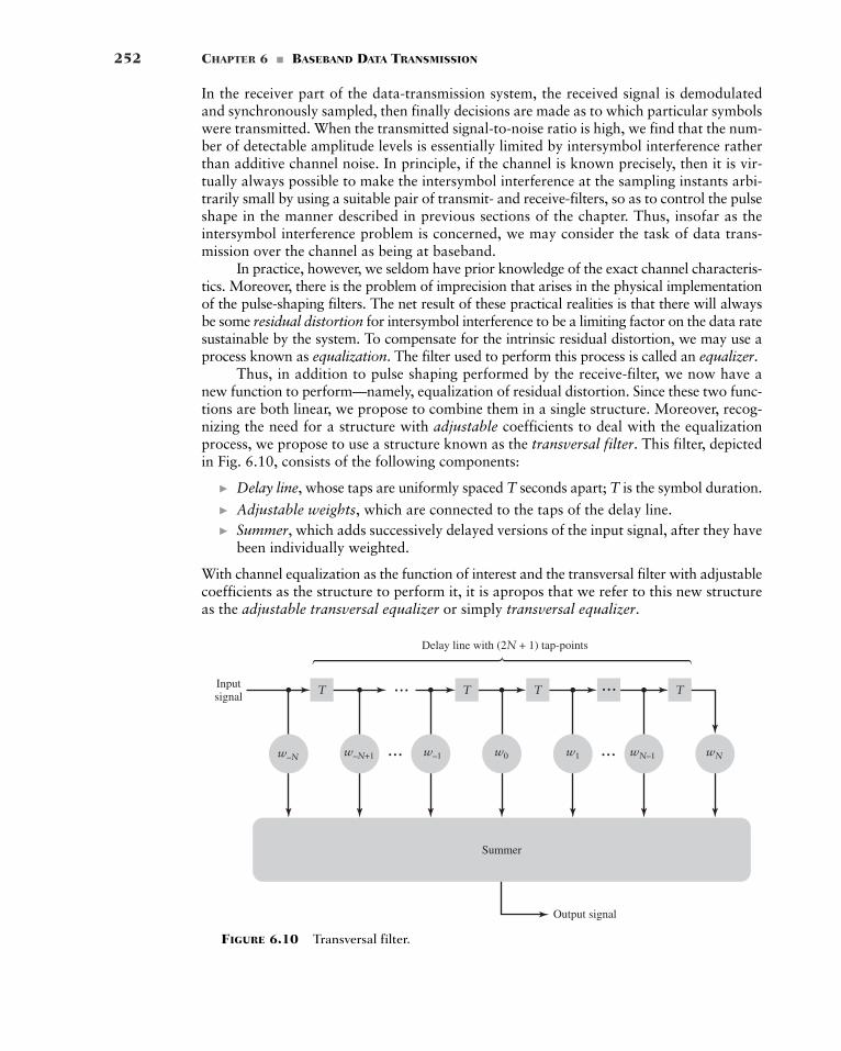
252 CHAPTER 6 � BASEBAND DATA TRANSMISSION
Output signal
Delay line with (2N + 1) tap-points
Summer
Inputsignal T
w–N w–N+1 wN–1 wNw–1 w1w0
...
... ...
T T ... T
FIGURE 6.10 Transversal filter.
In the receiver part of the data-transmission system, the received signal is demodulatedand synchronously sampled, then finally decisions are made as to which particular symbolswere transmitted. When the transmitted signal-to-noise ratio is high, we find that the num-ber of detectable amplitude levels is essentially limited by intersymbol interference ratherthan additive channel noise. In principle, if the channel is known precisely, then it is vir-tually always possible to make the intersymbol interference at the sampling instants arbi-trarily small by using a suitable pair of transmit- and receive-filters, so as to control the pulseshape in the manner described in previous sections of the chapter. Thus, insofar as theintersymbol interference problem is concerned, we may consider the task of data trans-mission over the channel as being at baseband.
In practice, however, we seldom have prior knowledge of the exact channel characteris-tics. Moreover, there is the problem of imprecision that arises in the physical implementationof the pulse-shaping filters. The net result of these practical realities is that there will alwaysbe some residual distortion for intersymbol interference to be a limiting factor on the data ratesustainable by the system. To compensate for the intrinsic residual distortion, we may use aprocess known as equalization. The filter used to perform this process is called an equalizer.
Thus, in addition to pulse shaping performed by the receive-filter, we now have anew function to perform—namely, equalization of residual distortion. Since these two func-tions are both linear, we propose to combine them in a single structure. Moreover, recog-nizing the need for a structure with adjustable coefficients to deal with the equalizationprocess, we propose to use a structure known as the transversal filter. This filter, depictedin Fig. 6.10, consists of the following components:
� Delay line, whose taps are uniformly spaced T seconds apart; T is the symbol duration.
� Adjustable weights, which are connected to the taps of the delay line.� Summer, which adds successively delayed versions of the input signal, after they have
been individually weighted.
With channel equalization as the function of interest and the transversal filter with adjustablecoefficients as the structure to perform it, it is apropos that we refer to this new structureas the adjustable transversal equalizer or simply transversal equalizer.
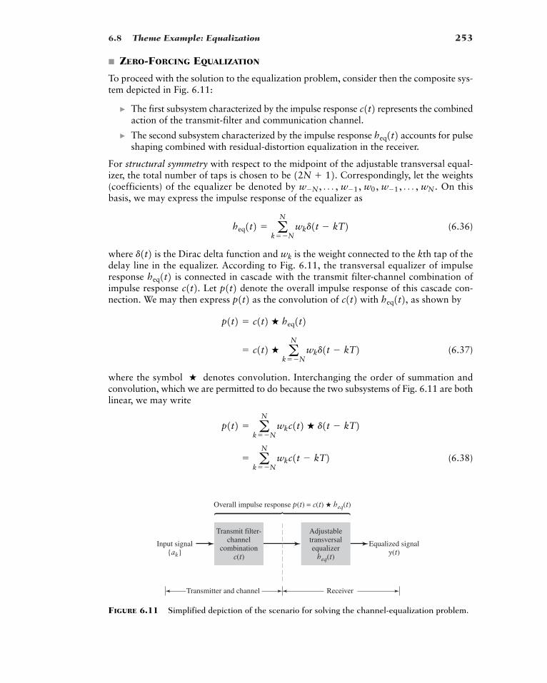
6.8 Theme Example: Equalization 253
� ZERO-FORCING EQUALIZATION
To proceed with the solution to the equalization problem, consider then the composite sys-tem depicted in Fig. 6.11:
� The first subsystem characterized by the impulse response represents the combinedaction of the transmit-filter and communication channel.
� The second subsystem characterized by the impulse response accounts for pulseshaping combined with residual-distortion equalization in the receiver.
For structural symmetry with respect to the midpoint of the adjustable transversal equal-izer, the total number of taps is chosen to be Correspondingly, let the weights(coefficients) of the equalizer be denoted by On thisbasis, we may express the impulse response of the equalizer as
(6.36)
where is the Dirac delta function and is the weight connected to the kth tap of thedelay line in the equalizer. According to Fig. 6.11, the transversal equalizer of impulseresponse is connected in cascade with the transmit filter-channel combination ofimpulse response Let denote the overall impulse response of this cascade con-nection. We may then express as the convolution of with as shown by
(6.37)
where the symbol denotes convolution. Interchanging the order of summation andconvolution, which we are permitted to do because the two subsystems of Fig. 6.11 are bothlinear, we may write
(6.38)� aN
k��Nwkc1t � kT2
p1t2 � aN
k��Nwkc1t2 � d1t � kT2
�
� c1t2 � aN
k��Nwkd1t � kT2
p1t2 � c1t2 � heq1t2heq1t2,c1t2p1t2p1t2c1t2.heq1t2
wkd1t2heq1t2 � a
N
k��Nwkd1t � kT2
w�N , Á , w�1, w0, w�1, Á , wN .12N 12.
heq1t2c1t2
Input signal{ak}
Equalized signaly(t)
Transmit filter-channel
combinationc(t)
Transmitter and channel
Adjustabletransversalequalizer
heq(t)
Overall impulse response p(t) = c(t) � heq(t)
Receiver
FIGURE 6.11 Simplified depiction of the scenario for solving the channel-equalization problem.
254 CHAPTER 6 � BASEBAND DATA TRANSMISSION
where, in the last line, we made use of the sifting property of the delta function. Evaluat-ing Eq. (6.38) at the sampling times we get the discrete convolution sum.
(6.39)
To simplify the presentation, let and We may then rewrite Eq.(6.39) in the compact form
(6.40)
Elimination of the intersymbol interference requires that we satisfy the Nyquist criterionfor distortionless transmission described in Eq. (6.11), on the basis of which we write
where E is the transmitted signal energy per symbol. From Eq. (6.40) we note that thereare only adjustable weights at our disposal. Hence, the Nyquist criterion fordistortionless transmission can only be approximately satisfied (depending on N) as follows:
(6.41)
Hence, imposing the condition of Eq. (6.39) on the discrete convolution sum of Eq. (6.40),we obtain a system of simultaneous equations:
(6.42)
Equivalently, in matrix form we may write
(6.43)
A transversal equalizer described by Eq. (6.42), or equivalently Eq. (6.43), is referred to asa zero-forcing equalizer, so called because the equalizer forces the intersymbol interferenceto be zero at sampling instants of the received signal. The zero-forcing equalizeris optimum in the sense that it minimizes the peak distortion in the absence of noise; peakdistortion is defined in Eq. (6.34). Another nice feature of the zero-forcing equalizer is thatit is relatively simple to implement. Moreover, in theory, the longer we make the equalizer(i.e., permit N to approach infinity), the more closely will the equalized system approachthe ideal condition specified by the Nyquist criterion for distortionless transmission across
12N 12
Gc0
Á c�N1 c�N c�N�1Á c�2N
o o o o o o ocN�1
Á c0 c�1 c�2Á c�N�1
cNÁ c1 c0 c�1
Á c�N
cN1Á c2 c1 c0
Á c�N1
o o o o o o oc2N
Á cN1 cN cN�1Á c0
W Gw�N
ow�1
w0
w1
owN
W � G0o02E0o0
W
aN
k��Nwkci�k � b2E , i � 0
0, i � �1, �2, Á , �N
12N 12
pi � b2E , i � 0 0, i � �1, �2, Á , �N
12N 12
pi � b2E , for i � 0 0, for all i 0
pi � aN
k��Nwkci�k
ci � c1iT2.pi � p1iT2p1iT2 � a
N
k��Nwkc11i � k2T2
t � iT,
6.8 Theme Example: Equalization 255
8The solution of Eq. (6.43), namely, the weights of the transversal equalizer, is defined by the inverseof the matrix of known coefficients on the left-hand side of the equation multiplied bythe highly sparse column vector on the right-hand side. For large N, computation of the inverse matrix becomestroublesome, in which case we have to seek another approach, for details, see Haykin (2001)
12N 12-by-12N 12 12N 12
the channel. Note, however, that since the zero-forcing equalizer ignores the effect of addi-tive channel noise, the equalized system does not always offer the best solution to the inter-symbol interference problem.7
� Drill Problem 6.6 Assume the following perfect conditions:
• The residual distortion in the data transmission system is zero.• The pulse shaping is partitioned equally between the transmit filter-channel combination
and the receiver.• The transversal equalizer is infinitely long.
(a) Find the corresponding value of the equalizer’s transfer function in terms of the overallpulse spectrum
(b) For the roll-off factor demonstrate that a transversal equalizer of infinite lengthwould essentially satisfy the perfect condition found in part (a) of the problem. �
� HOW COULD THE RECEIVER DETERMINE THE
Given the coefficients defining the sampled impulse responseof the transmit filter-channel combination, we may then use the simultaneous system ofequations (6.43) to solve for the corresponding weights of the transversal equal-izer.8 This computation, however, presumes that the receiver already has knowledge of theset of coefficients But, how can the receiver acquire this knowledge?
A commonly used method of addressing this fundamental question is to use a pilot-assisted training session that proceeds as follows:
1. For the binary data sequence applied to the transmitter input, use a determin-istic sequence of 1s and 0s that is noise-like in character, hence the reference to thissequence as a pseudo-noise (PN) sequence. The reason for using such a sequence asthe pilot is to provide a measure of uniqueness.
2. The PN sequence is known a priori to the receiver. Accordingly, with the receiversynchronized to the transmitter, the receiver is enabled to know when to initiate thetraining session.
3. Finally, knowing the transmitted PN sequence and measuring the corresponding chan-nel output, it is a straight-forward matter for the receiver to estimate the sequence representing the sampled impulse response of the transmit-filter and channel combined.
5ck6
5bk6
5ck6k��NN .
12N 12c�N , Á , c�1, c0, c1, Á , cN ,
5ck6?
a � 1,P1f2.
7For an equalizer more robust than the zero-forcing equalizer, we look to a different optimization criterion—namely,the mean-square error criterion—which accounts for the combined effects of residual distortion and channelnoise. The mean-square error (e.g., average error power) is defined as the expected value of the squared error (dif-ference) between the “desired” response and the “actual” response of the equalizer; expectation is a statistical oper-ator, the discussion of which is deferred to Chapter 8.
For detailed discussion of the minimum mean-square-error equalizer and its adaptive implementation, seeHaykin (2001). Unlike a fixed equalizer (i.e., a transversal equalizer whose tap weights are fixed once their indi-vidual adjustments have been computed), an adaptive equalizer is equipped with a mechanism that continuallyadjusts the tap weights of the equalizer so as to compensate for the time-varying nature of telephone and wire-less channels, which is another practical reality of digital communications.
256 CHAPTER 6 � BASEBAND DATA TRANSMISSION
6.9 Summary and Discussion
The subject of digital data transmission over a communication channel encompasses twodifferent families of applications, depending on the type of channel being considered:
(i) Baseband data transmission, for which the channel is of a low-pass type.
(ii) Band-pass data transmission, for which the channel is of a band-pass type. (Band-passdata transmission is also referred to as passband data transmission.)
In this chapter, we studied baseband data transmission. The study of band-pass data trans-mission is taken up in Chapter 7.
In particular, this chapter focused on the intersymbol interference problem, whicharises due to imperfections in the frequency response of the channel, assumed to be linear.With attention directed at a signal pulse of interest at the channel output, intersymbolinterference (ISI) refers to the effect on that pulse due to cross-talk or spillover from all othersignal pulses in the data stream applied to the channel input.
A corrective measure widely used in practice is to shape the overall pulse spectrumof the baseband system, starting from the source of the message signal all the way to thereceiver. The optimum solution for the pulse spectrum is provided by the Nyquist channel,which guarantees zero intersymbol interference at a bit rate equal to twice the channelbandwidth. However, this optimum solution to the intersymbol interference problem isunrealizable due to its brick-wall characterization. To circumvent the issue of unrealiz-ability, we may use the raised-cosine pulse spectrum, which provides design flexibilitythrough the roll-off factor that varies between zero and unity. Note, however, that the useof a nonzero roll-off factor is a necessary but not sufficient condition for physical realiz-ability of the solution to the zero-intersymbol interference problem. In addition, the raised-cosine pulse spectrum must be associated with a linear phase characteristic whose slopedepends on the roll-off factor, as discussed in Problem 6.4. It is also noteworthy that amore sophisticated solution to the intersymbol interference problem is provided by parti-tioning the overall task of pulse shaping equally between the transmitter and receiver, usingthe root raised-cosine pulse spectrum.
In this chapter, we also studied a practical issue closely related to intersymbol interference:how to evaluate it experimentally. The eye pattern is a tool that addresses this issue in a veryinsightful manner. Indeed, in a single picture, the eye pattern portrays the degrading effects oftiming jitter, intersymbol interference (due to system imperfections), and channel noise, all ofwhich are of a random nature. In this context, there is a basic difference between intersymbolinterference and noise. Intersymbol interference is a signal-dependent phenomenon; it thereforedisappears when the information-bearing signal is switched off. On the other hand, noise isalways there, regardless of whether there is data transmission or not.
One last comment is in order. In addition to pulse shaping, there is another correc-tive measure for dealing with the intersymbol interference problem—namely, channel equal-ization. This second corrective measure involves the use of a transversed filter withadjustable coefficients; the filter is placed in the receiver and adjusted in a principled man-ner so as to compensate for residual distortion resulting from imperfections in the chan-nel’s impulse response.
Additional Problems 257
ADDITIONAL PROBLEMS
6.7 Starting with Eq. (6.17) for the raised-cosine pulse spectrum use the inverse Fourier trans-form to derive the corresponding time response defined in Eq. (6.19).
6.8 The raised-cosine pulse spectrum for a roll-off factor of unity is given by
which is a special case of Eq. (6.17) for Show that the time response the inverseFourier transform of is
6.9 A computer puts out binary data at the rate of 56 kilobits per second. The computer output istransmitted using a baseband binary PAM system that is designed to have a raised-cosine pulsespectrum. Determine the transmission bandwidth required for each of the following roll-off factors:(a)(b)(c)(d)
6.10 A binary PAM wave is to be transmitted over a low-pass channel with bandwidth of 75 kHz.The bit duration is Find a raised-cosine pulse spectrum that satisfies these requirements.
6.11 Consider a channel with bandwidth 3.0 kHz, which is available for data transmission usingbinary PAM. Plot the permissible bit (signaling) rate versus the excess bandwidth assum-ing that the roll-off factor varies from zero to unity, and that the criterion for zero intersym-bol interference is satisfied.
6.12 You are given a channel of bandwidth 3.0 kHz. The requirement is to transmit data over thechannel at the rate of 4.5 kilobits/s using binary PAM.(a) What is the maximum roll-off factor in the raised-cosine pulse spectrum that can accom-
modate this data transmission?(b) What is the corresponding excess bandwidth?
6.13 This problem follows up on the pulse-shaping criterion for zero intersymbol interference, whichis embodied in Eq. (6.30). This criterion can be satisfied by an infinite number of overall pulsespectra denoted by The brick-wall spectrum of Fig. 6.2(a) and the raised-cosine pulsespectrum of Fig. 6.4(a) are two such examples. The pulse spectra shown in parts (a) and (b) ofFig. 6.12 are two other examples that can also satisfy the pulse-shaping criterion of Eq. (6.30).
(a) Derive the condition that the bandwidth in Fig. 6.12(a) must satisfy for the requirementof zero intersymbol interference to be satisfied for binary PAM.
(b) Repeat the problem for the pulse spectrum of Fig. 6.12(b).(c) Given the four pulse spectra, the two of Figs. 6.2(b) and 6.3(a) and those of Fig. 6.12, why
then is it that the raised-cosine pulse spectrum of Fig. 6.3(a) is the preferred choice in prac-tice? Justify your answer.
B0
P1f2.
a
fn,1>Tb
10 ms.
a � 1.0a � 0.75a � 0.5a � 0.25
p1t2 � 2Esinc14B0t2
1 � 16B02t2
P1f2, p1t2,a � 1.
P1f2 �c 2E
2B0cos2¢ pf
4B0≤ , 0 � ƒf ƒ � 2B0
0, 2B0 � ƒf ƒ
p1t2 P1f2,
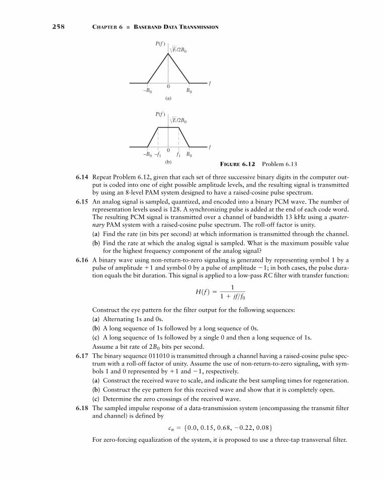
258 CHAPTER 6 � BASEBAND DATA TRANSMISSION
6.14 Repeat Problem 6.12, given that each set of three successive binary digits in the computer out-put is coded into one of eight possible amplitude levels, and the resulting signal is transmittedby using an 8-level PAM system designed to have a raised-cosine pulse spectrum.
6.15 An analog signal is sampled, quantized, and encoded into a binary PCM wave. The number ofrepresentation levels used is 128. A synchronizing pulse is added at the end of each code word.The resulting PCM signal is transmitted over a channel of bandwidth 13 kHz using a quater-nary PAM system with a raised-cosine pulse spectrum. The roll-off factor is unity.(a) Find the rate (in bits per second) at which information is transmitted through the channel.(b) Find the rate at which the analog signal is sampled. What is the maximum possible value
for the highest frequency component of the analog signal?6.16 A binary wave using non-return-to-zero signaling is generated by representing symbol 1 by a
pulse of amplitude and symbol 0 by a pulse of amplitude in both cases, the pulse dura-tion equals the bit duration. This signal is applied to a low-pass RC filter with transfer function:
Construct the eye pattern for the filter output for the following sequences:(a) Alternating 1s and 0s.(b) A long sequence of 1s followed by a long sequence of 0s.(c) A long sequence of 1s followed by a single 0 and then a long sequence of 1s.Assume a bit rate of bits per second.
6.17 The binary sequence 011010 is transmitted through a channel having a raised-cosine pulse spec-trum with a roll-off factor of unity. Assume the use of non-return-to-zero signaling, with sym-bols 1 and 0 represented by and respectively.(a) Construct the received wave to scale, and indicate the best sampling times for regeneration.(b) Construct the eye pattern for this received wave and show that it is completely open.(c) Determine the zero crossings of the received wave.
6.18 The sampled impulse response of a data-transmission system (encompassing the transmit filterand channel) is defined by
For zero-forcing equalization of the system, it is proposed to use a three-tap transversal filter.
cn � 50.0, 0.15, 0.68, �0.22, 0.086
�1,1
2B0
H1f2 �1
1 jf>f0
�1;1
P(f )
–B0 B00
(a)
f
/E/2B0
P(f )
–B0 –f1 f1 B00
(b)
f
/E/2B0
FIGURE 6.12 Problem 6.13
Advanced Problems 259
(a) Calculate the adjustable weights of the equalizer.(b) Using the equalizer determined in part (a), calculate the residual intersymbol interference at
the equalizer output.(c) Identify the magnitude of the sample making the largest contribution to the residual inter-
symbol interference.6.19 Repeat Problem 6.18, this time using a five-tap transversal filter for zero-forcing equalization
of the system. Compare the residual intersymbol interference at the output of the equalizer withthat in Problem 6.18, and comment on the benefit gained by using a longer transversal filter forthe equalization process.
ADVANCED PROBLEMS
The treatment of intersymbol interference presented in much of this chapter has viewed it as anundesirable phenomenon. Nevertheless, by adding intersymbol interference to the transmittedsignal in a controlled manner, it is possible to achieve a signaling rate of symbols per secondin a channel of bandwidth hertz. Such an approach is called correlative coding or partial-response signaling. The next four problems address issues related to correlative coding, assummarized here:
• Problems 6.20 and 6.21 pertain to duobinary signaling. In particular, Problem 6.20addresses the duobinary conversion filter, the use of which can lead to a propagation oferrors. To mitigate this problem, we use a precoder addressed in Problem 6.21.
• Problem 6.22 pertains to a modification of the schemes described in Problems 6.20 and6.21.
• Finally, Problem 6.23 probes the use of modified duobinary signaling for single sidebandmodulation applied to data transmission.
6.20 Figure 6.13 depicts the duobinary signaling scheme in its simplest form. The incoming binarysequence consists of uncorrelated binary symbols 1 and 0, each having duration Thissequence is first applied to a pulse-amplitude modulator to produce the two-level sequence consisting of pulses (short enough to be viewed as unit impulses). Specifically,
The two-level sequence is next applied to the duobinary conversion filter enclosed inside thedashed rectangle in Fig. 6.13, where the Nyquist channel is defined by (see Eq. (6.15))
Hopt1f2 � c 2E2B0
, for �B0 � f � B0
0, otherwise
Hopt1f25ak6ak � b1, if symbol bk is 1
�1, if symbol bk is 0
5ak6Tb .5bk6
B0
2B0
Sampleat t = kTb
DelayTb
Duobinary conversion filterH(f )
Input binarysequence
{bk}
Outputsequence
{ck}{ak}
Σ+
+
NyquistchannelHopt(f )
Pulse-amplitudemodulator
FIGURE 6.13 Problem 6.20
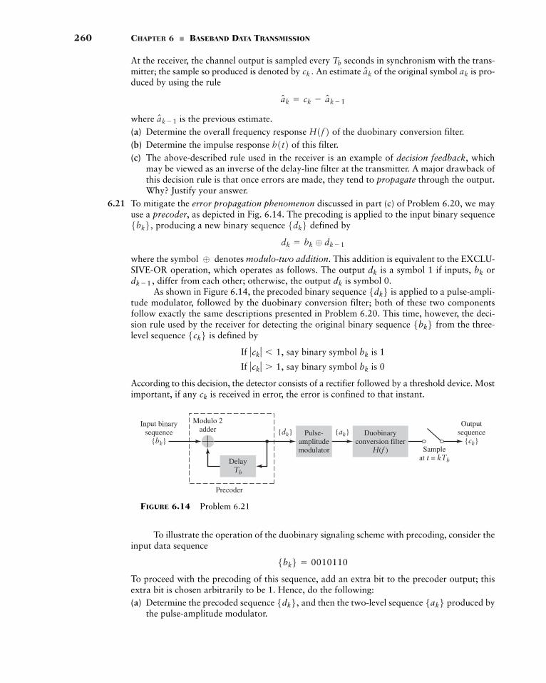
260 CHAPTER 6 � BASEBAND DATA TRANSMISSION
At the receiver, the channel output is sampled every seconds in synchronism with the trans-mitter; the sample so produced is denoted by An estimate of the original symbol is pro-duced by using the rule
where is the previous estimate.(a) Determine the overall frequency response of the duobinary conversion filter.(b) Determine the impulse response of this filter.(c) The above-described rule used in the receiver is an example of decision feedback, which
may be viewed as an inverse of the delay-line filter at the transmitter. A major drawback ofthis decision rule is that once errors are made, they tend to propagate through the output.Why? Justify your answer.
6.21 To mitigate the error propagation phenomenon discussed in part (c) of Problem 6.20, we mayuse a precoder, as depicted in Fig. 6.14. The precoding is applied to the input binary sequence
producing a new binary sequence defined by
where the symbol denotes modulo-two addition. This addition is equivalent to the EXCLU-SIVE-OR operation, which operates as follows. The output is a symbol 1 if inputs, or
differ from each other; otherwise, the output is symbol 0.As shown in Figure 6.14, the precoded binary sequence is applied to a pulse-ampli-
tude modulator, followed by the duobinary conversion filter; both of these two componentsfollow exactly the same descriptions presented in Problem 6.20. This time, however, the deci-sion rule used by the receiver for detecting the original binary sequence from the three-level sequence is defined by
If say binary symbol is 1
If say binary symbol is 0
According to this decision, the detector consists of a rectifier followed by a threshold device. Mostimportant, if any is received in error, the error is confined to that instant.ck
bkƒck ƒ � 1,
bkƒck ƒ � 1,
5ck6 5bk65dk6dkdk�1 ,
bkdk
⊕
dk � bk ⊕ dk�1
5dk65bk6,
h1t2 H1f2aN k�1
aN k � ck � aN k�1
akaNkck .Tb
Outputsequence
{ck}Sample
at t = kTb
{ak}Pulse-amplitudemodulator
Duobinaryconversion filter
H(f )
DelayTb
Precoder
Input binarysequence
{bk}{dk}
Modulo 2adder
FIGURE 6.14 Problem 6.21
To illustrate the operation of the duobinary signaling scheme with precoding, consider theinput data sequence
To proceed with the precoding of this sequence, add an extra bit to the precoder output; thisextra bit is chosen arbitrarily to be 1. Hence, do the following:(a) Determine the precoded sequence and then the two-level sequence produced by
the pulse-amplitude modulator.5ak65dk6,
5bk6 � 0010110
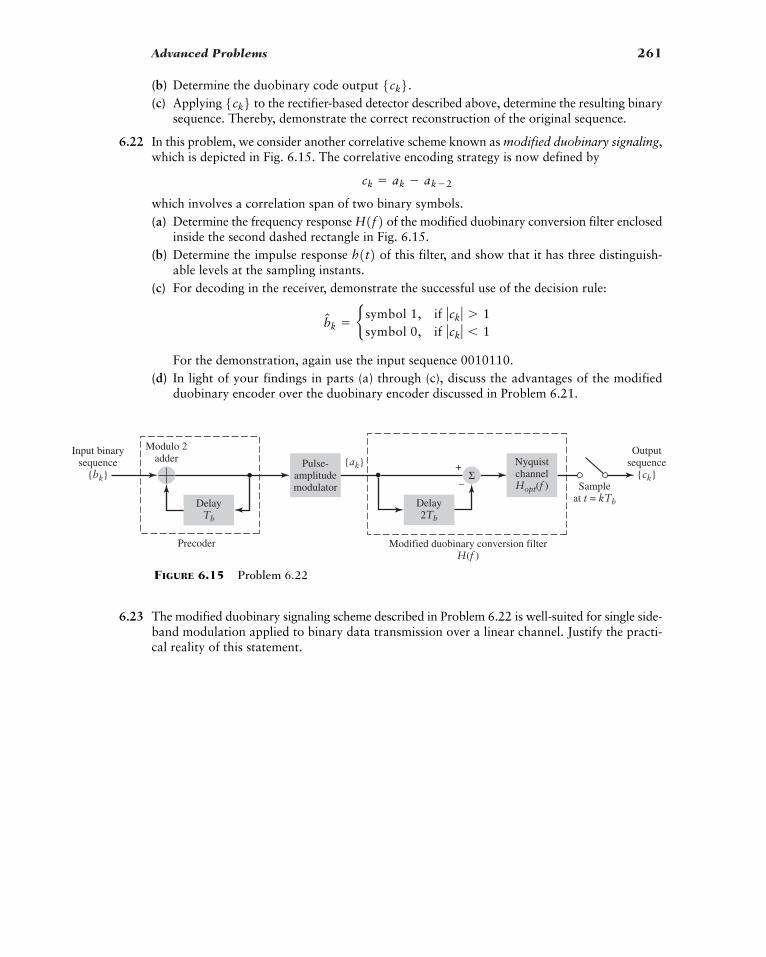
Advanced Problems 261
(b) Determine the duobinary code output (c) Applying to the rectifier-based detector described above, determine the resulting binary
sequence. Thereby, demonstrate the correct reconstruction of the original sequence.
6.22 In this problem, we consider another correlative scheme known as modified duobinary signaling,which is depicted in Fig. 6.15. The correlative encoding strategy is now defined by
which involves a correlation span of two binary symbols.(a) Determine the frequency response of the modified duobinary conversion filter enclosed
inside the second dashed rectangle in Fig. 6.15.(b) Determine the impulse response of this filter, and show that it has three distinguish-
able levels at the sampling instants.(c) For decoding in the receiver, demonstrate the successful use of the decision rule:
For the demonstration, again use the input sequence 0010110.(d) In light of your findings in parts (a) through (c), discuss the advantages of the modified
duobinary encoder over the duobinary encoder discussed in Problem 6.21.
bNk � b symbol 1, if ƒck ƒ � 1symbol 0, if ƒck ƒ � 1
h1t2H1f2ck � ak � ak�2
5ck65ck6.
6.23 The modified duobinary signaling scheme described in Problem 6.22 is well-suited for single side-band modulation applied to binary data transmission over a linear channel. Justify the practi-cal reality of this statement.
Outputsequence
{ck}Sample
at t = kTbDelay2Tb
Modified duobinary conversion filterH(f )
Σ+
–
NyquistchannelHopt(f )
{ak}Pulse-amplitudemodulator
DelayTb
Precoder
Input binarysequence
{bk}
Modulo 2adder
FIGURE 6.15 Problem 6.22
262
CHAPTER 7
DIGITAL BAND-PASS
MODULATION TECHNIQUES
In baseband data transmission, which we studied in Chapter 6, an incoming serial datastream is represented in the form of a discrete pulse-amplitude modulated wave that can betransmitted over a low-pass channel (e.g., a coaxial cable). What if the requirement is totransmit the data stream over a band-pass channel, exemplified by wireless and satellitechannels? In applications of this kind, we usually resort to the use of a modulation strat-egy configured around a sinusoidal carrier whose amplitude, phase, or frequency is variedin accordance with the information-bearing data stream. Digital modulation techniquesdealing with band-pass data transmission are studied in this chapter.
The primary aim of the chapter is to describe some important digital band-passmodulation techniques used in practice. In particular, we describe three basic modulationschemes: namely, amplitude-shift keying, phase-shift keying, and frequency-shift keying,followed by some of their variants. Another issue that will receive particular attention isthat of coherent versus noncoherent detection. A digital communication system is said tobe coherent if the receiver is synchronized to the transmitter with respect to carrier phase;otherwise, the system is said to be noncoherent. Naturally, a noncoherent system offersthe practical advantage of reduced complexity but at the cost of degraded performance.Considerations of the issue of noise performance evaluation are deferred to Chapter 10.
This chapter will teach us three lessons:
� Lesson 1: Each digital band-pass modulation scheme is defined by a transmitted signalwith a unique phasor representation.
� Lesson 2: At the receiving end, digital demodulation techniques encompass differentforms, depending on whether the receiver is coherent or noncoherent.
� Lesson 3: Two ways of classifying digital modulation schemes are (a) by the type of modu-lation used, and (b) whether the transmitted data stream is in binary or M-ary form.
7.1 Some Preliminaries
Given a binary source that emits symbols 0 and 1, the modulation process involves switch-ing or keying the amplitude, phase, or frequency of a sinusoidal carrier wave between a pairof possible values in accordance with symbols 0 and 1. To be more specific, consider thesinusoidal carrier
(7.1)c1t2 � Ac cos12pfct fc2
7.1 Some Preliminaries 263
where is the carrier amplitude, is the carrier frequency, and is the carrier phase. Giventhese three parameters of the carrier we may now identify three distinct forms ofbinary modulation:
1. Binary amplitude shift-keying (BASK), in which the carrier frequency and carrierphase are both maintained constant, while the carrier amplitude is keyed betweenthe two possible values used to represent symbols 0 and 1.
2. Binary phase-shift keying (BPSK), in which the carrier amplitude and carrier fre-quency are both maintained constant, while the carrier phase is keyed between the twopossible values (e.g., 0° and 180°) used to represent symbols 0 and 1.
3. Binary frequency-shift keying (BFSK), in which the carrier amplitude and carrierphase are both maintained constant, while the carrier frequency is keyed between thetwo possible values used to represent symbols 0 and 1.
In light of these definitions, we see that BASK, BPSK, and BFSK are special cases of ampli-tude modulation, phase modulation, and frequency modulation, respectively. Indeed, itwas with this close relationship between analog and digital modulation techniques in mindthat in the “Summary and Discussion” sections of Chapter 3 on amplitude modulationand Chapter 4 on angle modulation, we briefly highlighted the connections between ana-log and digital modulation schemes. An important conclusion that we can draw from theclose relationship between analog and digital modulation techniques is that despite theirbasic differences, BASK, BPSK, and BFSK share a common feature: all three of them areexamples of a band-pass process.
In the analog communications literature, the sinusoidal carrier is commonlydefined as in Eq. (7.1). On the other hand, in the digital communications literature, the usualpractice is to assume that the carrier has unit energy measured over one symbol (bit)duration. Specifically, from Problem 3.28, we recall that the carrier amplitude
(7.2)
where is the bit duration. Using the terminology of Eq. (7.2), we may thus express thecarrier in the equivalent form
(7.3)
From the material presented in Chapter 2 on the Fourier representation of signalsand systems, we learned that decreasing the duration of a rectangular pulse has the effectof widening the effective band of frequencies contained in the pulse. In a corresponding fash-ion, decreasing the bit duration has the effect of increasing the transmission bandwidthrequirement of a binary modulated wave.
One other lesson learned from material covered in previous chapters—namely, Chap-ters 3 and 4—is the fact that the transmission bandwidth requirement of an angle-modulatedwave is greater than that of the corresponding amplitude-modulated wave. In light of thatlesson, we may say that the transmission bandwidth requirement of BFSK is greater thanthat of BASK for a given binary source. However, the same does not hold for BPSK, as weshall see from the material presented in this chapter. This is one of many differences thatdistinguish digital modulation from analog modulation.
Tb
c1t2 � B 2Tb
cos12pfct fc2c1t2Tb
Ac � B 2Tb
c1t2c1t2
c1t2, fcfcAc
264 CHAPTER 7 � DIGITAL BAND-PASS MODULATION TECHNIQUES
� BAND-PASS ASSUMPTION
The spectrum of a digitally modulated wave, exemplified by BASK, BPSK and BFSK, iscentered on the carrier frequency implicitly or explicitly. Moreover, as with analog mod-ulation, it is normal practice to assume that the carrier frequency is large compared withthe “bandwidth” of the incoming binary data stream that acts as the modulating signal. Thisband-pass assumption has certain implications, as discussed next.
To be specific, consider a linear modulation scheme for which the modulated waveis defined by
(7.4)
where denotes an incoming binary wave. Then, setting the carrier phase forconvenience of presentation, we may use Eq. (7.3) to express the modulated wave as
(7.5)
Under the assumption where W is the bandwidth of the binary wave there will be no spectral overlap in the generation of (i.e., the spectral content ofthe modulated wave for positive frequencies is essentially separated from its spectralcontent for negative frequencies).
Another implication of the band-pass assumption is that we may express the trans-mitted signal energy per bit as
(7.6)
Using the trigonometric identity
we may rewrite Eq. (7.6) as
(7.7)
The band-pass assumption implies that is essentially constant over one completecycle of the sinusoidal wave cos which, in turn, means that
Accordingly, we may approximate Eq. (7.7) as
(7.8)
In words, for linear digital modulation schemes governed by Eq. (7.5), the transmitted sig-nal energy (on a per bit basis) is a scaled version of the energy in the incoming binary waveresponsible for modulating the sinusoidal carrier.
Eb �1Tb L
Tb
0ƒb1t2 ƒ2 dt
LT
b
0ƒb1t2 ƒ2 cos14pfct2 dt � 0
14pfct2, ƒb1t2 ƒ2
Eb �1Tb L
Tb
0ƒb1t2 ƒ2 dt
1Tb L
Tb
0ƒb1t2 ƒ2 cos14pfct2 dt
cos212pfct2 �1231 cos14pfct24
�2Tb L
Tb
0ƒb1t2 ƒ2 cos212pfct2 dt
Eb � LT
b
0ƒs1t2 ƒ2 dt
s1t2 b1t2,fc W W,
s1t2 � B 2Tb
b1t2 cos12pfct2s1t2fc � 0b1t2
s1t2 � b1t2c1t2
fcfc ,
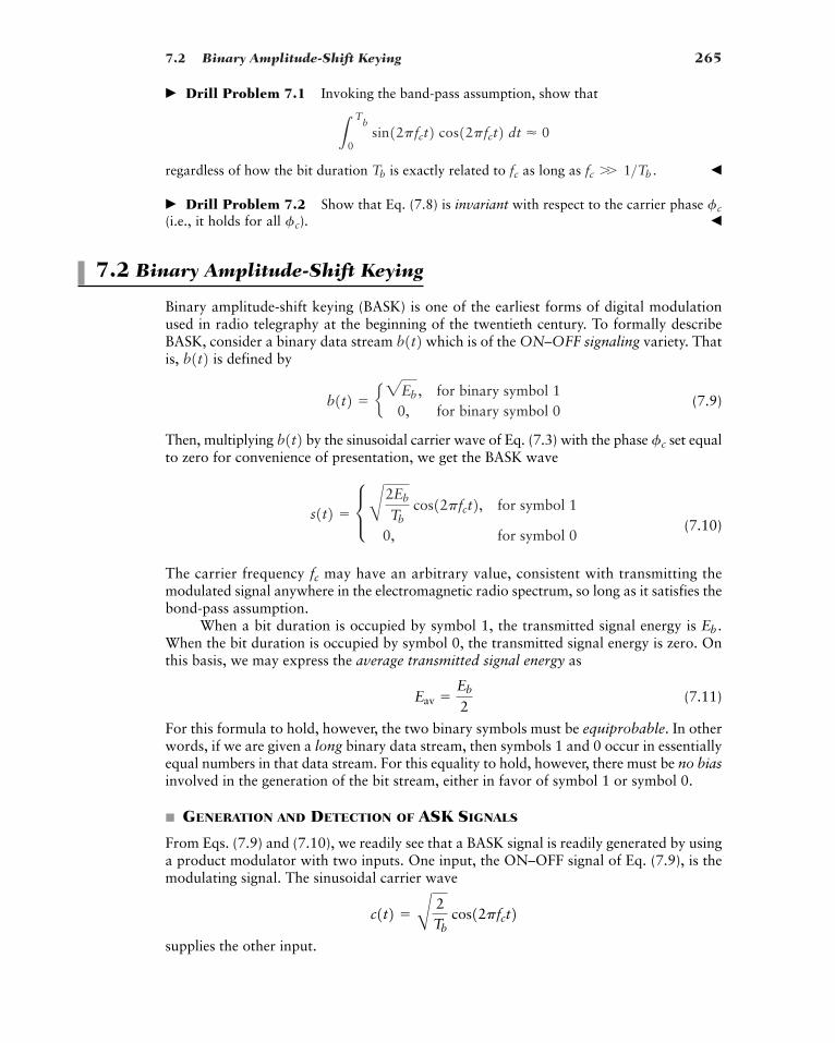
7.2 Binary Amplitude-Shift Keying 265
� Drill Problem 7.1 Invoking the band-pass assumption, show that
regardless of how the bit duration is exactly related to as long as �
� Drill Problem 7.2 Show that Eq. (7.8) is invariant with respect to the carrier phase (i.e., it holds for all ). �
7.2 Binary Amplitude-Shift Keying
Binary amplitude-shift keying (BASK) is one of the earliest forms of digital modulationused in radio telegraphy at the beginning of the twentieth century. To formally describeBASK, consider a binary data stream which is of the ON–OFF signaling variety. Thatis, is defined by
(7.9)
Then, multiplying by the sinusoidal carrier wave of Eq. (7.3) with the phase set equalto zero for convenience of presentation, we get the BASK wave
(7.10)
The carrier frequency may have an arbitrary value, consistent with transmitting themodulated signal anywhere in the electromagnetic radio spectrum, so long as it satisfies thebond-pass assumption.
When a bit duration is occupied by symbol 1, the transmitted signal energy is When the bit duration is occupied by symbol 0, the transmitted signal energy is zero. Onthis basis, we may express the average transmitted signal energy as
(7.11)
For this formula to hold, however, the two binary symbols must be equiprobable. In otherwords, if we are given a long binary data stream, then symbols 1 and 0 occur in essentiallyequal numbers in that data stream. For this equality to hold, however, there must be no biasinvolved in the generation of the bit stream, either in favor of symbol 1 or symbol 0.
� GENERATION AND DETECTION OF ASK SIGNALS
From Eqs. (7.9) and (7.10), we readily see that a BASK signal is readily generated by usinga product modulator with two inputs. One input, the ON–OFF signal of Eq. (7.9), is themodulating signal. The sinusoidal carrier wave
supplies the other input.
c1t2 � B 2Tb
cos12pfct2
Eav �Eb
2
Eb .
fc
s1t2 � c B2Eb
Tb cos12pfct2, for symbol 1
0, for symbol 0
fcb1t2b1t2 � e2Eb , for binary symbol 1
0, for binary symbol 0
b1t2 b1t2
fc
fc
fc W 1>Tb .fcTb
LT
b
0 sin12pfct2 cos12pfct2 dt � 0
266 CHAPTER 7 � DIGITAL BAND-PASS MODULATION TECHNIQUES
Input binarysequence
0 0 1 1 0 1 1 0 0 1
(b) t
(c)
(a)
t
(d) t
A property of BASK that is immediately apparent from Fig. 7.1(b), which depicts theBASK waveform corresponding to the incoming binary data stream of Fig. 7.1(a), is the non-constancy of the envelope of the modulated wave. Accordingly, insofar as detection of theBASK wave is concerned, the simplest way is to use an envelope detector, exploiting the non-constant-envelope property of the BASK signal.
� COMPUTER EXPERIMENT I: SPECTRAL ANALYSIS OF BASK
Consider a binary data stream that consists of a square wave, the amplitude of whichalternates between the constant levels and zero every seconds. The square waveis centered on the origin for convenience of the presentation. The objective of the exper-iment is twofold:
(i) To investigate the effect of varying the carrier frequency on the power spectrum ofthe BASK signal assuming that the square wave is fixed. Recall that the powerspectrum of a signal (expressed in decibels) is defined as 10 times the logarithm (tobase 10) of the squared magnitude (amplitude) spectrum of the signal.
(ii) To investigate the effect of varying the frequency of the square wave on the spectrumof the BASK signal, assuming that the sinusoidal carrier wave is fixed.
For the purpose of computer evaluation, we set the carrier frequency where n isan integer. This choice of the carrier frequency permits the simulation of a band-passsystem on a digital computer without requiring the only restriction on thechoice is to make sure that spectral overlap is avoided. (We follow this practice whenperforming computer experiments as we go forward in the study of other digital modula-tion schemes.)
fc W 1>Tb ;fc
fc � n>Tb
s1t2, fc
Tb2Eb
FIGURE 7.1 The three basic forms of signaling binary information. (a) Binary datastream. (b) Amplitude-shift keying. (c) Phase-shift keying. (d) Frequency-shift keyingwith continuous phase.
7.2 Binary Amplitude-Shift Keying 267
To plot the power spectra (in decibels) of the digitally modulated waves (in this exper-iment and others to follow), we use the fast Fourier transform (FFT) algorithm, which wasdiscussed in Section 2.10. The simulation parameters used in the computer experiments (thisone and the subsequent experiments) are as follows:
Number of data bits (1s and 0s)
Sampling frequency,
Number of data points (samples)
Block size of the FFT, N
Results of the computation are plotted in Figs. 7.2 and 7.3.The two parts of Fig. 7.2 correspond to objective (i) of the experiment. Specifically,
the two plots shown in Fig. 7.2 correspond to the following parameters:
Bit duration,
Carrier frequency,
The second set of results plotted in Fig. 7.3 corresponds to objective (ii) of the experiment,using the following parameters:
Carrier frequency,
Bit duration,
In each part of Figs. 7.2 and 7.3, we show two power spectral plots: one shaded,resulting from the computation, and the other, well-defined curve, obtained from theory.(We follow a similar practice in the computer experiments to follow.) Here we must rec-ognize that the binary data streams used in the experiments are of finite length, hence thejagged appearance depicted in the figures. In contrast, theory leads to a solid curve, whichclosely follows the “envelope” of the computational results.
In light of the results plotted in Figs. 7.2 and 7.3, we can make the followingobservations for positive frequencies:
1. The spectrum of the BASK signal contains a line component at
2. When the square wave is fixed and the carrier frequency is doubled, the mid-bandfrequency of the BASK signal is likewise doubled.
3. When the carrier is fixed and the bit duration is halved, the width of the main lobeof the sinc function defining the envelope of the BASK spectrum is doubled, which,in turn, means that the transmission bandwidth of the BASK signal is doubled.
4. The transmission bandwidth of BASK, measured in terms of the width of the mainlobe of its spectrum, is equal to where is the bit duration.
These observations support the statement: the BASK signal is an example of amplitudemodulation that includes the carrier wave as a component in its composition.
Tb2>Tb ,
f � fc .
Tb � c 1 s for Fig. 7.31a212
s for Fig 7.31b2
fc � 8 Hz
fc � b 4 Hz for Fig. 7.21a28 Hz for Fig. 7.21b2
Tb � 1 s
� 4096
� 100 fs � 10,000 data points
� 100 Hzfs
� 100
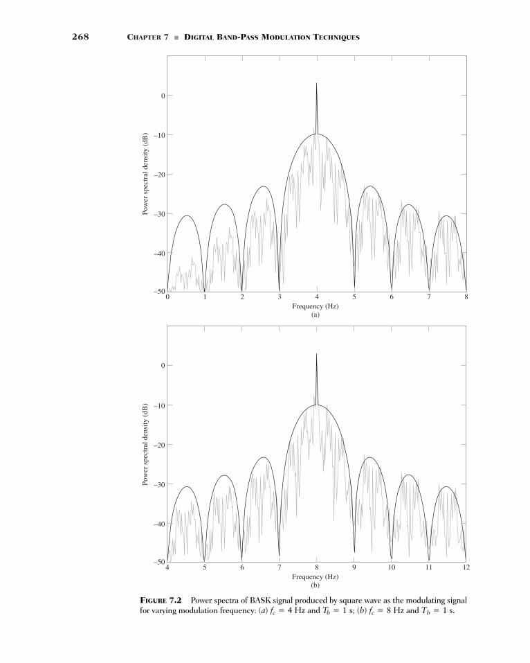
268 CHAPTER 7 � DIGITAL BAND-PASS MODULATION TECHNIQUES
0 81 2 3 4 5 6 7
Pow
er s
pect
ral d
ensi
ty (
dB)
–50
Frequency (Hz)(a)
–40
–30
–20
–10
0
FIGURE 7.2 Power spectra of BASK signal produced by square wave as the modulating signalfor varying modulation frequency: (a) and ; (b) and Tb � 1 s.fc � 8 HzTb � 1 sfc � 4 Hz
4 125 6 7 8 9 10 11
Pow
er s
pect
ral d
ensi
ty (
dB)
–50
Frequency (Hz)(b)
–40
–30
–20
–10
0
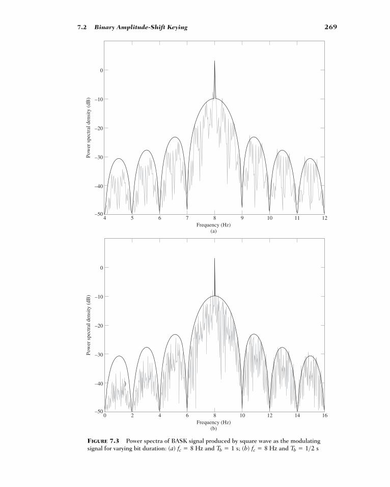
7.2 Binary Amplitude-Shift Keying 269
0 162 4 6 8 10 12 14
Pow
er s
pect
ral d
ensi
ty (
dB)
–50
Frequency (Hz)(b)
–40
–30
–20
–10
0
)
4 125 6 7 8 9 10 11
Pow
er s
pect
ral d
ensi
ty (
dB)
–50
Frequency (Hz)(a)
–40
–30
–20
–10
0
FIGURE 7.3 Power spectra of BASK signal produced by square wave as the modulatingsignal for varying bit duration: (a) and ; (b) and Tb � 1>2 sfc � 8 HzTb � 1 sfc � 8 Hz
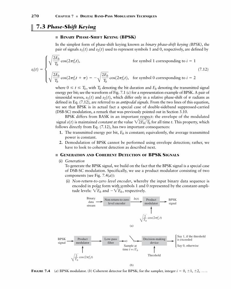
270 CHAPTER 7 � DIGITAL BAND-PASS MODULATION TECHNIQUES
7.3 Phase-Shift Keying
� BINARY PHASE-SHIFT KEYING (BPSK)
In the simplest form of phase-shift keying known as binary phase-shift keying (BPSK), thepair of signals and used to represent symbols 1 and 0, respectively, are defined by
(7.12)
where with denoting the bit duration and denoting the transmitted signalenergy per bit; see the waveform of Fig. 7.1 (c) for a representation example of BPSK. A pair ofsinusoidal waves, and which differ only in a relative phase-shift of radians asdefined in Eq. (7.12), are referred to as antipodal signals. From the two lines of this equation,we see that BPSK is in actual fact a special case of double-sideband suppressed-carried (DSB-SC) modulation, a remark that was previously pointed out in Section 3.10.
BPSK differs from BASK in an important respect: the envelope of the modulatedsignal is maintained constant at the value for all time t. This property, whichfollows directly from Eq. (7.12), has two important consequences:
1. The transmitted energy per bit, is constant; equivalently, the average transmittedpower is constant.
2. Demodulation of BPSK cannot be performed using envelope detection; rather, wehave to look to coherent detection as described next.
� GENERATION AND COHERENT DETECTION OF BPSK SIGNALS
(i) GenerationTo generate the BPSK signal, we build on the fact that the BPSK signal is a special caseof DSB-SC modulation. Specifically, we use a product modulator consisting of twocomponents (see Fig. 7.4(a)):(i) Non-return-to-zero level encoder, whereby the input binary data sequence is
encoded in polar form with symbols 1 and 0 represented by the constant-ampli-tude levels: and respectively.�2Eb ,2Eb
Eb
22Eb>Tbs1t2
ps21t2,s11t2EbTb0 � t � Tb ,
si1t2 � e B2Eb
Tb cos12pfct2, for symbol 1 corresponding to i � 1
B2Eb
Tb cos12pfct p2 � �B2Eb
Tb cos12pfct2, for symbol 0 corresponding to i � 2
s21t2s11t2
(a)
(b)
D2
Tb
Non-return-to-zerolevel encoder
Productmodulator
cos(2�fc t)
BPSKsignal
Sample attime t = iTb
b(t)Binarydata
stream
—
Productmodulator
Low-passfilter
Decision-makingdevice
Say 1, if the thresholdis exceeded
Say 0, otherwise
BPSKsignal
D2
Tbcos(2�fct)
Threshold—
FIGURE 7.4 (a) BPSK modulator. (b) Coherent detector for BPSK; for the sampler, integer i � 0, �1, �2, Á .
7.3 Phase-Shift Keying 271
(ii) Product modulator, which multiplies the level-encoded binary wave by the sinu-soidal carrier of amplitude to produce the BPSK signal.
The timing pulses used to generate the level-encoded binary wave and the sinusoidalcarrier wave are usually, but not necessarily, extracted from a common master clock.
(ii) DetectionTo detect the original binary sequence of 1s and 0s, the BPSK signal at the channeloutput is applied to a receiver that consists of four sections, as depicted in Fig. 7.4(b):(i) Product modulator, which is also supplied with a locally generated reference
signal that is a replica of the carrier wave (ii) Low-pass filter, designed to remove the double-frequency components of the
product modulator output (i.e., the components centered on ) and pass thezero-frequency components.
(iii) Sampler, which uniformly samples the output of the low-pass filter at where ; the local clock governing the operation of the sampleris synchronized with the clock responsible for bit-timing in the transmitter.
(iv) Decision-making device, which compares the sampled value of the low-pass filter’soutput to an externally supplied threshold, every seconds. If the threshold isexceeded, the device decides in favor of symbol 1; otherwise, it decides in favorof symbol 0.
The BPSK receiver described in Fig. 7.4 is said to be coherent in the sense that the sinu-soidal reference signal applied to the product modulator in the demodulator is synchronousin phase (and, of course, frequency) with the carrier wave used in the modulator. Thisrequirement can be achieved by using a phase-locked loop, which was described in Section4.8. In addition to synchrony with respect to carrier phase, the receiver also has an accu-rate knowledge of the interval occupied by each binary symbol.
The operation of the coherent BPSK receiver in Fig. 7.4(b) follows a procedure sim-ilar to that described for the demodulation of a double-sideband suppressed-carrier (DSB-SC) modulated wave (described in Section 3.3) with a couple of important additions:sampler and decision-making device. The rationale for this similarity builds on what we havealready stated: BPSK is simply another form of DSB-SC modulation.
However, an issue that needs particular attention is how to design the low-pass filterin Fig. 7.4(b). Specifically, what should the bandwidth of the filter be? From the conclu-sion drawn from the graphical results presented in Fig. 2.28 on the response of an ideal low-pass filter to an input rectangular pulse for varying time-bandwidth product, we recall thata time-bandwidth product equal to or greater than unity is a necessary requirement toensure that the waveform of the filter input is recognizable from the resulting output. Forthe problem at hand, we may therefore state that the bandwidth of the low-pass filter inthe coherent BPSK receiver of Fig. 7.4(b) has to be equal to or greater than the reciprocalof the bit duration for satisfactory operation of the receiver.
� COMPUTER EXPERIMENT II: SPECTRAL ANALYSIS OF BPSK
As with the experiment on BASK, consider a binary data stream that consists of a squarewave, the amplitude of which alternates between and every seconds. Thesquare wave is centered on the origin. The objectives of this second experiment are simi-lar to those of Computer Experiment I on BASK:
(i) To evaluate the effect of varying the carrier frequency on the power spectrum of theBPSK signal, for a fixed square modulating wave.
(ii) To evaluate the effect of varying modulation frequency on the power spectrum of theBPSK signal for a fixed carrier frequency.
fc
Tb�2Eb2Eb
Tb
Tb
i � 0, �1, �2, Át � i Tb,
2fc
c1t2.
x1t2
22>Tbc1t2
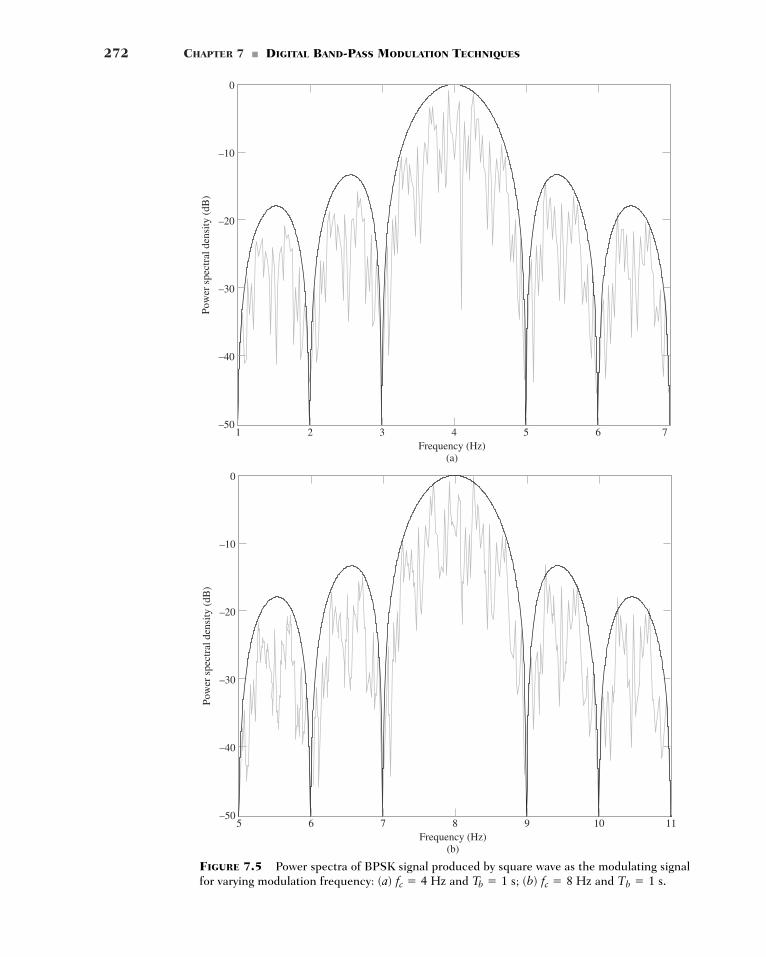
272 CHAPTER 7 � DIGITAL BAND-PASS MODULATION TECHNIQUES
1 72 3 4 5 6
Pow
er s
pect
ral d
ensi
ty (
dB)
–50
Frequency (Hz)(a)
–40
–30
–20
–10
0
FIGURE 7.5 Power spectra of BPSK signal produced by square wave as the modulating signalfor varying modulation frequency: (a) and ; (b) and Tb � 1 s.fc � 8 HzTb � 1 sfc � 4 Hz
5 116 7 8 9 10
Pow
er s
pect
ral d
ensi
ty (
dB)
–50
Frequency (Hz)(b)
–40
–30
–20
–10
0
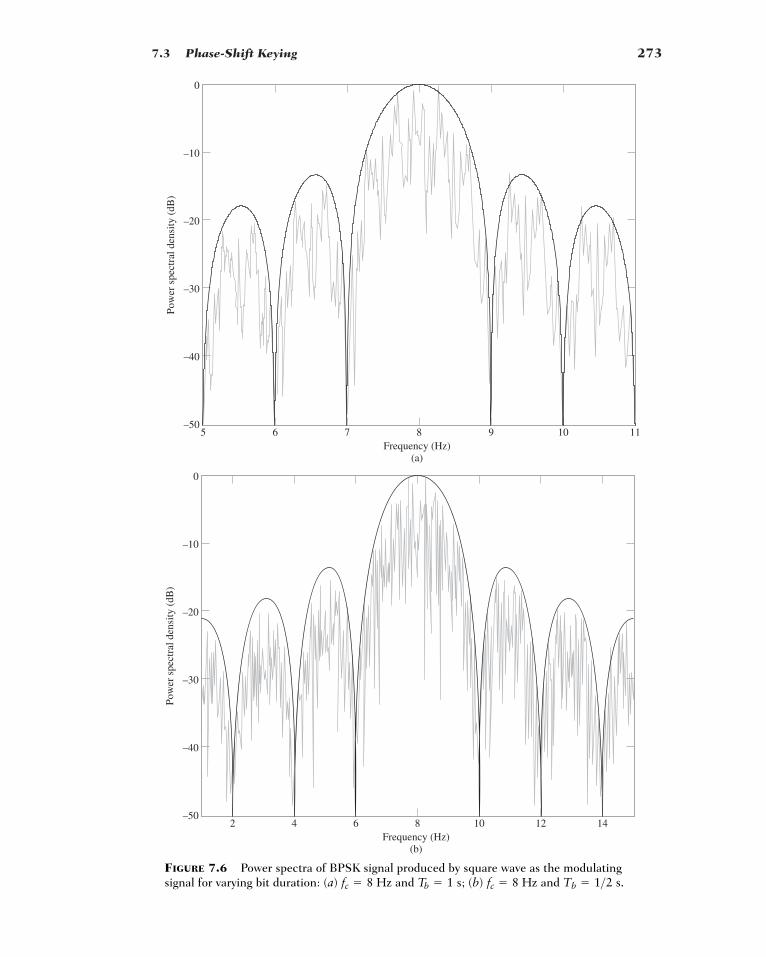
7.3 Phase-Shift Keying 273
5 116 7 8 9 10
Pow
er s
pect
ral d
ensi
ty (
dB)
–50
Frequency (Hz)(a)
–40
–30
–20
–10
0
FIGURE 7.6 Power spectra of BPSK signal produced by square wave as the modulatingsignal for varying bit duration: (a) and ; (b) and Tb � 1>2 s.fc � 8 HzTb � 1 sfc � 8 Hz
2 4 6 8 10 12 14
Pow
er s
pect
ral d
ensi
ty (
dB)
–50
Frequency (Hz)(b)
–40
–30
–20
–10
0
274 CHAPTER 7 � DIGITAL BAND-PASS MODULATION TECHNIQUES
To be consistent with Experiment I on BASK, objectives (i) and (ii) are investigated for thesame sets of frequencies used in that experiment. The results of the experiment on BPSKare plotted in Figs. 7.5 and 7.6, where, as before, we show computational results along-side the corresponding theoretical ones. Comparing these two figures with Figs. 7.2 and 7.3for BASK, respectively, we can make two important observations:
1. BASK and BPSK signals occupy the same transmission bandwidth—namely, —which defines the width of the main lobe of the sinc-shaped power spectra.
2. The BASK spectrum includes a carrier component, whereas this component is absentfrom the BPSK spectrum. With this observation we are merely restating the fact thatBASK is an example of amplitude modulation, whereas BPSK is an example of doublesideband-suppressed carrier modulation.
This second observation has practical implications of its own:
� The presence of carrier in the BASK spectrum means that the binary data stream canbe recovered by envelope detection of the BASK signal.
� On the other hand, suppression of the carrier in the BPSK spectrum mandates the useof coherent detection for recovery of the binary data stream from the BASK signal,as discussed on page 271.
� QUADRIPHASE-SHIFT KEYING
An important goal of digital communication is the efficient utilization of channel band-width. This goal is attained by a bandwidth-conserving modulation scheme known asquadriphase-shift keying, which builds on the same idea as that of quadrature-carriermultiplexing that was discussed in Section 3.5.
In quadriphase-shift keying (QPSK), as with BPSK, information carried by the trans-mitted signal is contained in the phase of a sinusoidal carrier. In particular, the phase of thesinusoidal carrier takes on one of four equally spaced values, such as and For this set of values, we define the transmitted signal as
(7.13)
where is the transmitted signal energy per symbol and T is the symbolduration. Each one of the four equally spaced phase values corresponds to a unique pairof bits called a dibit. For example, we may choose the foregoing set of phase values to rep-resent the Gray encoded set of dibits: 10, 00, 01, and 11. In this form of encoding, we seethat only a single bit is changed from one dibit to the next. Note that the symbol duration(i.e., the duration of each dibit) is twice the bit duration, as shown by
(7.14)
Using a well-known trigonometric identity, we may recast the transmitted signal in theinterval in the expanded form
(7.15)
where Based on the expanded form of Eq. (7.15), we can make some impor-tant observations:
1. In reality, the QPSK signal consists of the sum of two BPSK signals.
2. One BPSK signal, represented by the first term 22E>T cos312i � 12p>44 cos312pfct24,
i � 1, 2, 3, 4.
si1t2 � A2ET
cos c12i � 12p4d cos12pfct2 � A2E
T sin c12i � 12p
4d sin12pfct2
0 � t � T
T � 2Tb
i � 1, 2, 3, 4; E
si1t2 � cA2ET
cos c2pfct 12i � 12p4d , 0 � t � T
0, elsewhere
7p>4.p>4, 3p>4, 5p>4,
2>Tb
7.3 Phase-Shift Keying 275
defines the product of modulating a binary wave by the sinusoidal carrierwhich has unit energy over the symbol duration T. We also rec-
ognize that
(7.16)
We therefore see that this binary wave has an amplitude equal to
3. The other BPSK signal, represented by the second term
defines the product of modulating a different binary wave by the sinusoidal carrierwhich also has unit energy per symbol. This time, we recognize that
(7.17)
We therefore see that this second binary wave also has an amplitude equal to albeit in a different way with respect to the index i.
4. The two binary waves defined in Eqs. (7.16) and (7.17) share a common value for thesymbol duration—namely, T.
5. The two sinusoidal carrier waves identified under points 2 and 3 are in phase quad-rature with respect to each other. Moreover, they both have unit energy per symbolduration. We may therefore state that these two carrier waves constitute an ortho-normal pair of basis functions.
6. For each possible value of the index i, Eqs. (7.16) and (7.17) identity the corre-sponding dibit, as outlined in Table 7.1. This table also includes other related entriespertaining to the phase of the QPSK signal, and the amplitudes of the two binarywaves identified under points 2 and 3.
�2E>2,
�2E sin c12i � 12p4d � e�2E>2 for i � 1, 22E>2 for i � 3, 4
22>T sin12pfct2,�22E>T sin c12i � 12p
4d sin12pfct2,
�2E>2.
2E cos c12i � 12p4d � e 2E>2 for i � 1, 4
�2E>2 for i � 2, 3
22>T cos12pfct2,
TABLE 7.1 Relationship Between Index i And Identity of CorrespondingDibit, and Other Related Matters
Amplitudes of constituentbinary waves
Phase of QPSK signal Binary wave 1 Binary wave 2 Input dibit
Index i (radians)
1 10
2 00
3 01
4 112E>22E>27p>42E>2�2E>25p>4�2E>2�2E>23p>4�2E>22E>2p>4
0 � t � Ta21t2a11t2
� GENERATION AND COHERENT DETECTION OF QPSK SIGNALS
In light of the six points summarized above as well as the material presented previously inthis section on BPSK, we may construct the block diagrams depicted in Fig. 7.7 for thegeneration and coherent detection of QPSK signals, as described here:
(i) GenerationTo generate the QPSK signal, the incoming binary data stream is first converted intopolar form by a non-return-to-zero level encoder; the encoder output is denoted by b1t2.
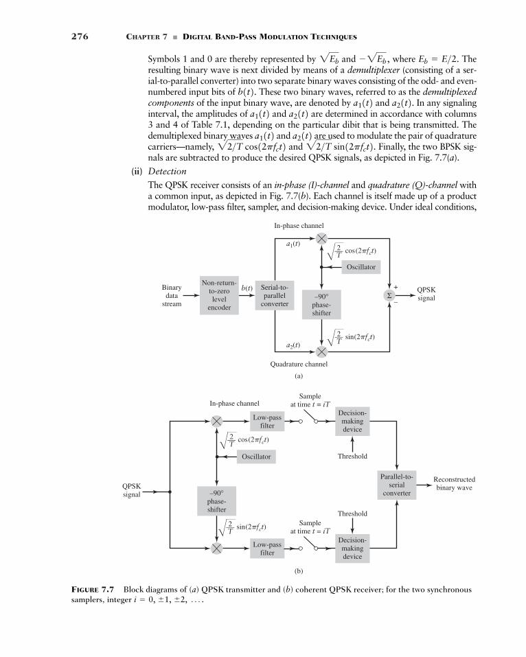
276 CHAPTER 7 � DIGITAL BAND-PASS MODULATION TECHNIQUES
(a)
D2T
cos(2�fct)a1(t)
a2(t)
—
D2T
sin(2�fct)—
Non-return-to-zerolevel
encoder
Serial-to-parallel
converter
Quadrature channel
In-phase channel
–90°phase-shifter
Binarydata
stream
b(t)Σ
+
–
Oscillator
QPSKsignal
(b)
In-phase channel
D2T
cos(2�fct)—
D2T
sin(2�fct)—
–90°phase-shifter
Low-passfilter
Decision-makingdevice
Threshold
Threshold
Parallel-to-serial
converter
Reconstructedbinary wave
Low-passfilter
QPSKsignal
Oscillator
Decision-makingdevice
Sampleat time t = iT
Sampleat time t = iT
FIGURE 7.7 Block diagrams of (a) QPSK transmitter and (b) coherent QPSK receiver; for the two synchronoussamplers, integer i � 0, �1, �2, Á .
Symbols 1 and 0 are thereby represented by and where Theresulting binary wave is next divided by means of a demultiplexer (consisting of a ser-ial-to-parallel converter) into two separate binary waves consisting of the odd- and even-numbered input bits of These two binary waves, referred to as the demultiplexedcomponents of the input binary wave, are denoted by and In any signalinginterval, the amplitudes of and are determined in accordance with columns3 and 4 of Table 7.1, depending on the particular dibit that is being transmitted. Thedemultiplexed binary waves and are used to modulate the pair of quadraturecarriers—namely, and Finally, the two BPSK sig-nals are subtracted to produce the desired QPSK signals, as depicted in Fig. 7.7(a).
(ii) Detection
The QPSK receiver consists of an in-phase (I)-channel and quadrature (Q)-channel witha common input, as depicted in Fig. 7.7(b). Each channel is itself made up of a productmodulator, low-pass filter, sampler, and decision-making device. Under ideal conditions,
22>T sin12pfct2.22>T cos12pfct2 a21t2a11t2a21t2a11t2 a21t2.a11t2b1t2.
Eb � E>2.�2Eb ,2Eb
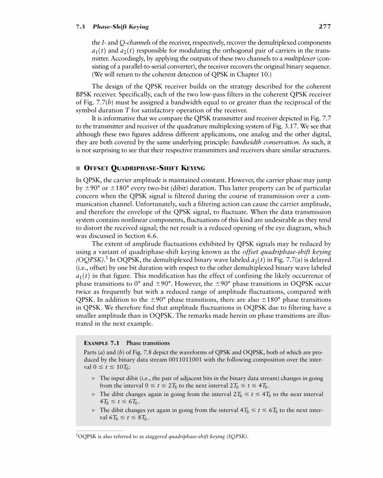
7.3 Phase-Shift Keying 277
1OQPSK is also referred to as staggered quadriphase-shift keying (SQPSK).
the I- and Q-channels of the receiver, respectively, recover the demultiplexed componentsand responsible for modulating the orthogonal pair of carriers in the trans-
mitter. Accordingly, by applying the outputs of these two channels to a multiplexer (con-sisting of a parallel-to-serial converter), the receiver recovers the original binary sequence.(We will return to the coherent detection of QPSK in Chapter 10.)
The design of the QPSK receiver builds on the strategy described for the coherentBPSK receiver. Specifically, each of the two low-pass filters in the coherent QPSK receiverof Fig. 7.7(b) must be assigned a bandwidth equal to or greater than the reciprocal of thesymbol duration T for satisfactory operation of the receiver.
It is informative that we compare the QPSK transmitter and receiver depicted in Fig. 7.7to the transmitter and receiver of the quadrature multiplexing system of Fig. 3.17. We see thatalthough these two figures address different applications, one analog and the other digital,they are both covered by the same underlying principle: bandwidth conservation. As such, itis not surprising to see that their respective transmitters and receivers share similar structures.
� OFFSET QUADRIPHASE-SHIFT KEYING
In QPSK, the carrier amplitude is maintained constant. However, the carrier phase may jumpby or every two-bit (dibit) duration. This latter property can be of particularconcern when the QPSK signal is filtered during the course of transmission over a com-munication channel. Unfortunately, such a filtering action can cause the carrier amplitude,and therefore the envelope of the QPSK signal, to fluctuate. When the data transmissionsystem contains nonlinear components, fluctuations of this kind are undesirable as they tendto distort the received signal; the net result is a reduced opening of the eye diagram, whichwas discussed in Section 6.6.
The extent of amplitude fluctuations exhibited by QPSK signals may be reduced byusing a variant of quadriphase-shift keying known as the offset quadriphase-shift keying(OQPSK).1 In OQPSK, the demultiplexed binary wave labeled in Fig. 7.7(a) is delayed(i.e., offset) by one bit duration with respect to the other demultiplexed binary wave labeled
in that figure. This modification has the effect of confining the likely occurrence ofphase transitions to 0° and However, the phase transitions in OQPSK occurtwice as frequently but with a reduced range of amplitude fluctuations, compared withQPSK. In addition to the phase transitions, there are also phase transitionsin QPSK. We therefore find that amplitude fluctuations in OQPSK due to filtering have asmaller amplitude than in OQPSK. The remarks made herein on phase transitions are illus-trated in the next example.
EXAMPLE 7.1 Phase transitions
Parts (a) and (b) of Fig. 7.8 depict the waveforms of QPSK and OQPSK, both of which are pro-duced by the binary data stream 0011011001 with the following composition over the inter-val
� The input dibit (i.e., the pair of adjacent bits in the binary data stream) changes in goingfrom the interval to the next interval
� The dibit changes again in going from the interval to the next interval
� The dibit changes yet again in going from the interval to the next inter-val 6Tb � t � 8Tb .
4Tb � t � 6Tb
4Tb � t � 6Tb .2Tb � t � 4Tb
2Tb � t � 4Tb .0 � t � 2Tb
0 � t � 10Tb:
�180°�90°
�90°�90°.a11t2
a21t2
�180°�90°
a21t2a11t2
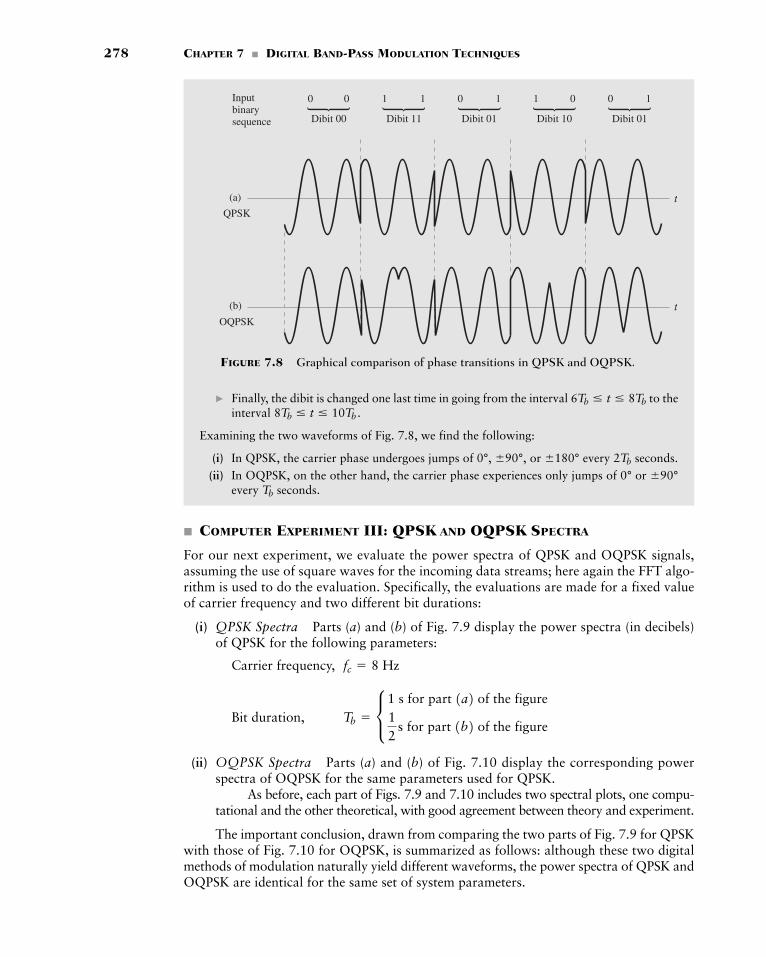
� Finally, the dibit is changed one last time in going from the interval to theinterval
Examining the two waveforms of Fig. 7.8, we find the following:
(i) In QPSK, the carrier phase undergoes jumps of 0°, or every seconds.(ii) In OQPSK, on the other hand, the carrier phase experiences only jumps of 0° or
every seconds.
� COMPUTER EXPERIMENT III: QPSK AND OQPSK SPECTRA
For our next experiment, we evaluate the power spectra of QPSK and OQPSK signals,assuming the use of square waves for the incoming data streams; here again the FFT algo-rithm is used to do the evaluation. Specifically, the evaluations are made for a fixed valueof carrier frequency and two different bit durations:
(i) QPSK Spectra Parts (a) and (b) of Fig. 7.9 display the power spectra (in decibels)of QPSK for the following parameters:
Carrier frequency,
Bit duration,
(ii) OQPSK Spectra Parts (a) and (b) of Fig. 7.10 display the corresponding powerspectra of OQPSK for the same parameters used for QPSK.
As before, each part of Figs. 7.9 and 7.10 includes two spectral plots, one compu-tational and the other theoretical, with good agreement between theory and experiment.
The important conclusion, drawn from comparing the two parts of Fig. 7.9 for QPSKwith those of Fig. 7.10 for OQPSK, is summarized as follows: although these two digitalmethods of modulation naturally yield different waveforms, the power spectra of QPSK andOQPSK are identical for the same set of system parameters.
Tb � c 1 s for part 1a2 of the figure12
s for part 1b2 of the figure
fc � 8 Hz
Tb
�90°2Tb�180°�90°,
8Tb � t � 10Tb .6Tb � t � 8Tb
278 CHAPTER 7 � DIGITAL BAND-PASS MODULATION TECHNIQUES
Inputbinarysequence Dibit 00 Dibit 11 Dibit 01 Dibit 10 Dibit 01
0 0 1 1 0 1 1 0 0 1
t(a)
QPSK
OQPSK
t(b)
FIGURE 7.8 Graphical comparison of phase transitions in QPSK and OQPSK.
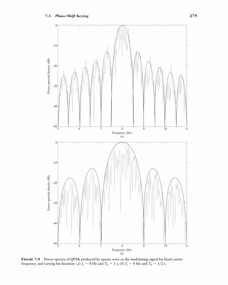
7.3 Phase-Shift Keying 279
5 6 7 8 9 10 11
Pow
er s
pect
ral d
ensi
ty (
dB)
–50
Frequency (Hz)(a)
–40
–30
–20
–10
0
5 6 7 8 9 10 11
Pow
er s
pect
ral d
ensi
ty (
dB)
–50
Frequency (Hz)(b)
–40
–30
–20
–10
0
FIGURE 7.9 Power spectra of QPSK produced by square wave as the modulating signal for fixed carrierfrequency and varying bit duration: (a) and (b) and Tb � 1>2 s.fc � 8 HzTb � 1 s;fc � 8 Hz
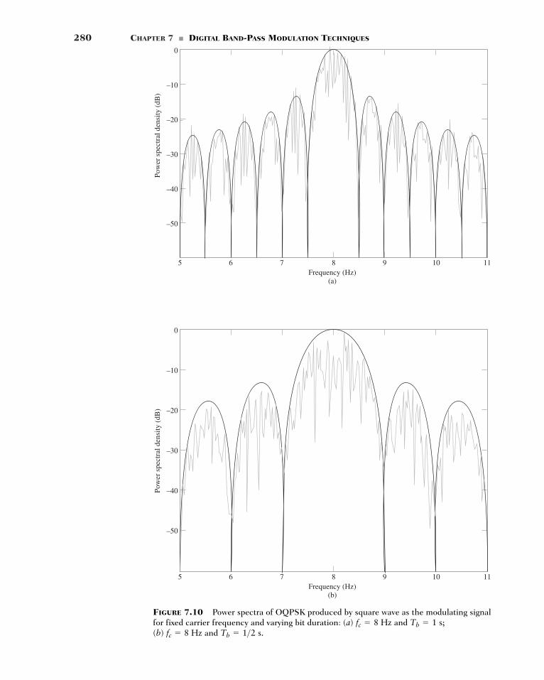
280 CHAPTER 7 � DIGITAL BAND-PASS MODULATION TECHNIQUES
5 6 7 8 9 10 11
Pow
er s
pect
ral d
ensi
ty (
dB)
Frequency (Hz)(a)
0
–10
–20
–30
–40
–50
FIGURE 7.10 Power spectra of OQPSK produced by square wave as the modulating signalfor fixed carrier frequency and varying bit duration: (a) and (b) and Tb � 1>2 s.fc � 8 Hz
Tb � 1 s;fc � 8 Hz
5 6 7 8 9 10 11
Pow
er s
pect
ral d
ensi
ty (
dB)
Frequency (Hz)(b)
–40
–50
–30
–20
–10
0
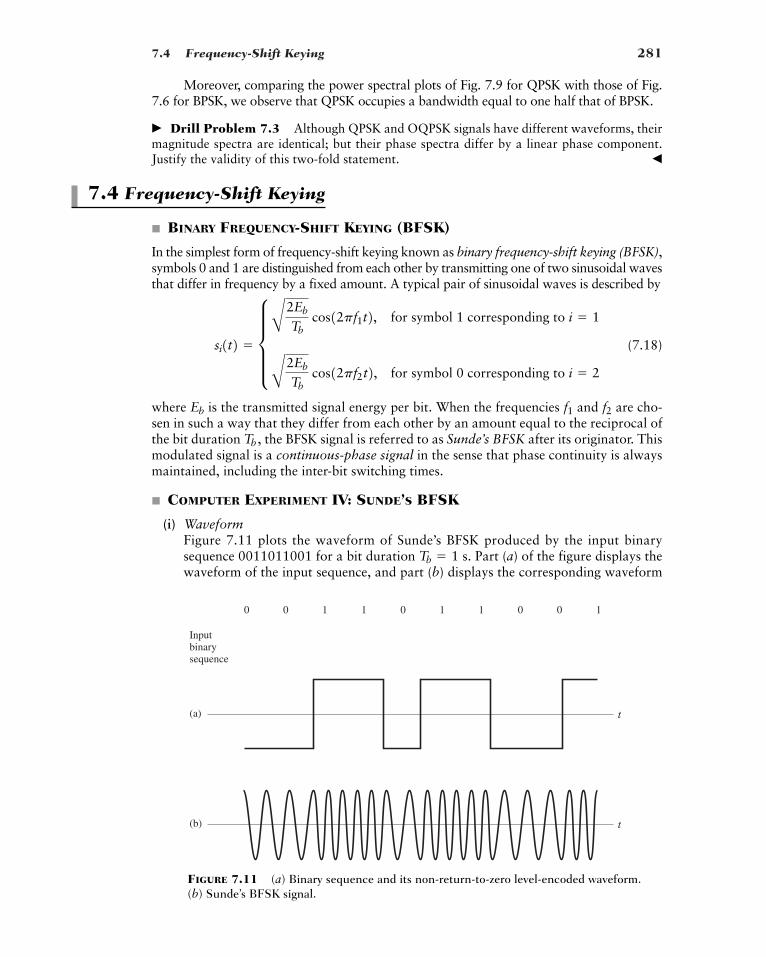
7.4 Frequency-Shift Keying 281
Moreover, comparing the power spectral plots of Fig. 7.9 for QPSK with those of Fig.7.6 for BPSK, we observe that QPSK occupies a bandwidth equal to one half that of BPSK.
� Drill Problem 7.3 Although QPSK and OQPSK signals have different waveforms, theirmagnitude spectra are identical; but their phase spectra differ by a linear phase component.Justify the validity of this two-fold statement. �
7.4 Frequency-Shift Keying
� BINARY FREQUENCY-SHIFT KEYING (BFSK)
In the simplest form of frequency-shift keying known as binary frequency-shift keying (BFSK),symbols 0 and 1 are distinguished from each other by transmitting one of two sinusoidal wavesthat differ in frequency by a fixed amount. A typical pair of sinusoidal waves is described by
(7.18)
where is the transmitted signal energy per bit. When the frequencies and are cho-sen in such a way that they differ from each other by an amount equal to the reciprocal ofthe bit duration the BFSK signal is referred to as Sunde’s BFSK after its originator. Thismodulated signal is a continuous-phase signal in the sense that phase continuity is alwaysmaintained, including the inter-bit switching times.
� COMPUTER EXPERIMENT IV: SUNDE’S BFSK
(i) WaveformFigure 7.11 plots the waveform of Sunde’s BFSK produced by the input binarysequence 0011011001 for a bit duration Part (a) of the figure displays thewaveform of the input sequence, and part (b) displays the corresponding waveform
Tb � 1 s.
Tb ,
f2f1Eb
si1t2 � e B2Eb
Tb cos12pf1t2, for symbol 1 corresponding to i � 1
B2Eb
Tb cos12pf2t2, for symbol 0 corresponding to i � 2
Inputbinarysequence
0 0 1 1 0 1 1 0 0 1
t(a)
t(b)
FIGURE 7.11 (a) Binary sequence and its non-return-to-zero level-encoded waveform. (b) Sunde’s BFSK signal.
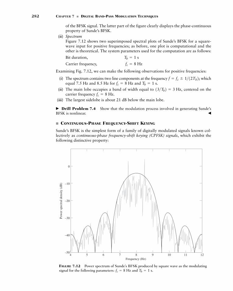
282 CHAPTER 7 � DIGITAL BAND-PASS MODULATION TECHNIQUES
4 5 6 7 8 9 10 11 12
Pow
er s
pect
ral d
ensi
ty (
dB)
–50
Frequency (Hz)
–30
–40
–20
–10
0
FIGURE 7.12 Power spectrum of Sunde’s BFSK produced by square wave as the modulatingsignal for the following parameters: and Tb � 1 s.fc � 8 Hz
of the BFSK signal. The latter part of the figure clearly displays the phase-continuousproperty of Sunde’s BFSK.
(ii) SpectrumFigure 7.12 shows two superimposed spectral plots of Sunde’s BFSK for a square-wave input for positive frequencies; as before, one plot is computational and theother is theoretical. The system parameters used for the computation are as follows:
Bit duration,
Carrier frequency,
Examining Fig. 7.12, we can make the following observations for positive frequencies:
(i) The spectrum contains two line components at the frequency whichequal 7.5 Hz and 8.5 Hz for and
(ii) The main lobe occupies a band of width equal to centered on thecarrier frequency
(iii) The largest sidelobe is about 21 dB below the main lobe.
� Drill Problem 7.4 Show that the modulation process involved in generating Sunde’sBFSK is nonlinear. �
� CONTINUOUS-PHASE FREQUENCY-SHIFT KEYING
Sunde’s BFSK is the simplest form of a family of digitally modulated signals known col-lectively as continuous-phase frequency-shift keying (CPFSK) signals, which exhibit thefollowing distinctive property:
fc � 8 Hz.13>Tb2 � 3 Hz,
Tb � 1 s.fc � 8 Hzf � fc � 1>12Tb2;
fc � 8 Hz
Tb � 1 s
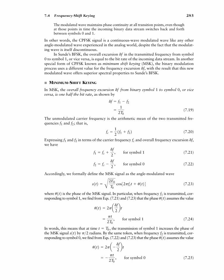
7.4 Frequency-Shift Keying 283
The modulated wave maintains phase continuity at all transition points, even thoughat those points in time the incoming binary data stream switches back and forthbetween symbols 0 and 1.
In other words, the CPFSK signal is a continuous-wave modulated wave like any otherangle-modulated wave experienced in the analog world, despite the fact that the modulat-ing wave is itself discontinuous.
In Sunde’s BFSK, the overall excursion in the transmitted frequency from symbol0 to symbol 1, or vice versa, is equal to the bit rate of the incoming data stream. In anotherspecial form of CPFSK known as minimum shift keying (MSK), the binary modulationprocess uses a different value for the frequency excursion with the result that this newmodulated wave offers superior spectral properties to Sunde’s BFSK.
� MINIMUM-SHIFT KEYING
In MSK, the overall frequency excursion from binary symbol 1 to symbol 0, or viceversa, is one half the bit rate, as shown by
(7.19)
The unmodulated carrier frequency is the arithmetic mean of the two transmitted fre-quencies and that is,
(7.20)
Expressing and in terms of the carrier frequency and overall frequency excursion we have
(7.21)
(7.22)
Accordingly, we formally define the MSK signal as the angle-modulated wave
(7.23)
where is the phase of the MSK signal. In particular, when frequency is transmitted, cor-responding to symbol 1, we find from Eqs. (7.21) and (7.23) that the phase assumes the value
(7.24)
In words, this means that at time the transmission of symbol 1 increases the phase ofthe MSK signal by radians. By the same token, when frequency is transmitted, cor-responding to symbol 0, we find from Eqs. (7.22) and (7.23) that the phase assumes the value
(7.25)� �pt2Tb
, for symbol 0
u1t2 � 2pa�df
2b t
u1t2f2p>2s1t2 t � Tb ,
�pt2Tb
, for symbol 1
u1t2 � 2padf2b t
u1t2f1u1t2s1t2 � B2Eb
Tb cos32pfct u1t24
f2 � fc �df
2, for symbol 0
f1 � fc df
2, for symbol 1
df,fcf2f1
fc �121f1 f22
f2;f1
�1
2Tb
df � f1 � f2
df
df,
df
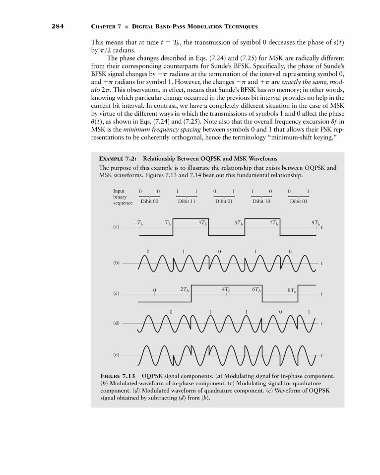
284 CHAPTER 7 � DIGITAL BAND-PASS MODULATION TECHNIQUES
This means that at time the transmission of symbol 0 decreases the phase of by radians.
The phase changes described in Eqs. (7.24) and (7.25) for MSK are radically differentfrom their corresponding counterparts for Sunde’s BFSK. Specifically, the phase of Sunde’sBFSK signal changes by radians at the termination of the interval representing symbol 0,and radians for symbol 1. However, the changes and are exactly the same, mod-ulo This observation, in effect, means that Sunde’s BFSK has no memory; in other words,knowing which particular change occurred in the previous bit interval provides no help in thecurrent bit interval. In contrast, we have a completely different situation in the case of MSKby virtue of the different ways in which the transmissions of symbols 1 and 0 affect the phase
as shown in Eqs. (7.24) and (7.25). Note also that the overall frequency excursion inMSK is the minimum frequency spacing between symbols 0 and 1 that allows their FSK rep-resentations to be coherently orthogonal, hence the terminology “minimum-shift keying.”
EXAMPLE 7.2: Relationship Between OQPSK and MSK Waveforms
The purpose of this example is to illustrate the relationship that exists between OQPSK andMSK waveforms. Figures 7.13 and 7.14 bear out this fundamental relationship:
dfu1t2,
2p.p�pp
�p
p>2 s1t2t � Tb ,
Inputbinarysequence Dibit 00 Dibit 11
–Tb Tb 3Tb
0 2Tb 4Tb 6Tb 8Tb
5Tb 7Tb 9Tb
Dibit 01 Dibit 10 Dibit 01
0 0 1 1 0 1 1 0 0 1
t(a)
0 0 01 1
0 01 1 1
t(b)
t(d)
t(c)
t(e)
FIGURE 7.13 OQPSK signal components: (a) Modulating signal for in-phase component.(b) Modulated waveform of in-phase component. (c) Modulating signal for quadraturecomponent. (d) Modulated waveform of quadrature component. (e) Waveform of OQPSKsignal obtained by subtracting (d) from (b).
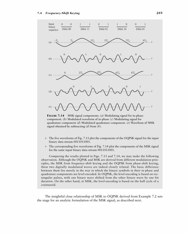
7.4 Frequency-Shift Keying 285
� The five waveforms of Fig. 7.13 plot the components of the OQPSK signal for the inputbinary data stream 0011011001.
� The corresponding five waveforms of Fig. 7.14 plot the components of the MSK signalfor the same input binary data stream 0011011001.
Comparing the results plotted in Figs. 7.13 and 7.14, we may make the followingobservation. Although the OQPSK and MSK are derived from different modulation prin-ciples, the MSK from frequency-shift keying and the OQPSK from phase-shift keying,these two digitally modulated waves are indeed closely related. The basic differencebetween them lies merely in the way in which the binary symbols in their in-phase andquadrature components are level-encoded. In OQPSK, the level-encoding is based on rec-tangular pulses, with one binary wave shifted from the other binary wave by one bitduration. On the other hand, in MSK, the level-encoding is based on the half cycle of acosinusoid.
The insightful close relationship of MSK to OQPSK derived from Example 7.2 setsthe stage for an analytic formulation of the MSK signal, as described next.
Inputbinarysequence Dibit 00 Dibit 11 Dibit 01 Dibit 10 Dibit 01
0 0 1 1 0 1 1 0 0 1
t(a)–Tb Tb 3Tb 5Tb 7Tb 9Tb
t(b)
t(c)2Tb0
0 1 0 1 0
0 011 1
4Tb 6Tb 8Tb
t(d)
t(e)
FIGURE 7.14 MSK signal components: (a) Modulating signal for in-phasecomponent. (b) Modulated waveform of in-phase (c) Modulating signal forquadrature component (d) Modulated quadrature component. (e) Waveform of MSKsignal obtained by subtracting (d) from (b).
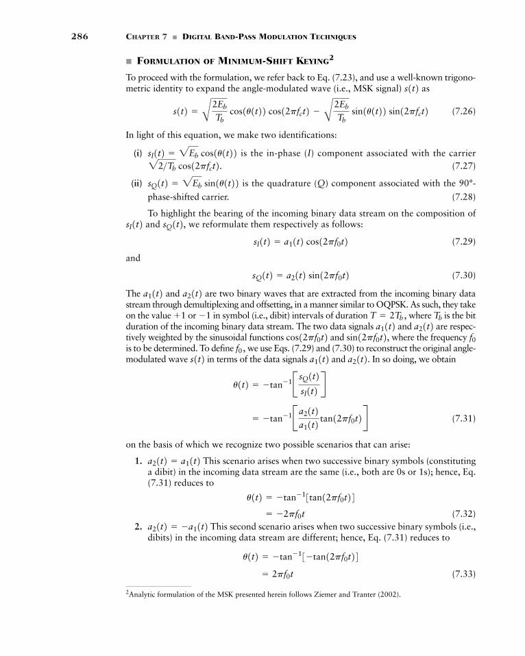
286 CHAPTER 7 � DIGITAL BAND-PASS MODULATION TECHNIQUES
� FORMULATION OF MINIMUM-SHIFT KEYING2
To proceed with the formulation, we refer back to Eq. (7.23), and use a well-known trigono-metric identity to expand the angle-modulated wave (i.e., MSK signal) as
(7.26)
In light of this equation, we make two identifications:
(i) is the in-phase (I) component associated with the carrier(7.27)
(ii) is the quadrature (Q) component associated with the 90°-
phase-shifted carrier. (7.28)
To highlight the bearing of the incoming binary data stream on the composition ofand we reformulate them respectively as follows:
(7.29)
and
(7.30)
The and are two binary waves that are extracted from the incoming binary datastream through demultiplexing and offsetting, in a manner similar to OQPSK. As such, they takeon the value or in symbol (i.e., dibit) intervals of duration where is the bitduration of the incoming binary data stream. The two data signals and are respec-tively weighted by the sinusoidal functions and where the frequency is to be determined. To define we use Eqs. (7.29) and (7.30) to reconstruct the original angle-modulated wave in terms of the data signals and In so doing, we obtain
(7.31)
on the basis of which we recognize two possible scenarios that can arise:
1. This scenario arises when two successive binary symbols (constitutinga dibit) in the incoming data stream are the same (i.e., both are 0s or 1s); hence, Eq.(7.31) reduces to
(7.32)2. This second scenario arises when two successive binary symbols (i.e.,
dibits) in the incoming data stream are different; hence, Eq. (7.31) reduces to
(7.33)� 2pf0t
u1t2 � �tan�13�tan12pf0t24a21t2 � �a11t2
� �2pf0t
u1t2 � �tan�13tan12pf0t24
a21t2 � a11t2
� �tan�1Ba21t2a11t2 tan12pf0t2R
u1t2 � �tan�1B sQ1t2sI1t2 R
a21t2.a11t2s1t2 f0,f0sin12pf0t2,cos12pf0t2 a21t2a11t2 TbT � 2Tb ,�11
a21t2a11t2sQ1t2 � a21t2 sin12pf0t2sI1t2 � a11t2 cos12pf0t2
sQ1t2,sI1t2
sQ1t2 � 2Eb sin1u1t2222>Tb cos12pfct2.sI1t2 � 2Eb cos1u1t22
s1t2 � B2Eb
Tb cos1u1t22 cos12pfct2 � B2Eb
Tb sin1u1t22 sin12pfct2
s1t2
2Analytic formulation of the MSK presented herein follows Ziemer and Tranter (2002).
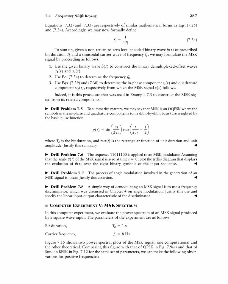
7.4 Frequency-Shift Keying 287
Equations (7.32) and (7.33) are respectively of similar mathematical forms as Eqs. (7.25)and (7.24). Accordingly, we may now formally define
(7.34)
To sum up, given a non-return-to-zero level encoded binary wave of prescribedbit duration and a sinusoidal carrier wave of frequency we may formulate the MSKsignal by proceeding as follows:
1. Use the given binary wave to construct the binary demultiplexed-offset wavesand
2. Use Eq. (7.34) to determine the frequency
3. Use Eqs. (7.29) and (7.30) to determine the in-phase component and quadraturecomponent respectively from which the MSK signal follows.
Indeed, it is this procedure that was used in Example 7.3 to construct the MSK sig-nal from its related components.
� Drill Problem 7.5 To summarize matters, we may say that MSK is an OQPSK where thesymbols in the in-phase and quadrature components (on a dibit-by-dibit basis) are weighted bythe basic pulse function
where is the bit duration, and rect(t) is the rectangular function of unit duration and unitamplitude. Justify this summary. �
� Drill Problem 7.6 The sequence 11011100 is applied to an MSK modulator. Assumingthat the angle of the MSK signal is zero at time plot the trellis diagram that displaysthe evolution of over the eight binary symbols of the input sequence. �
� Drill Problem 7.7 The process of angle modulation involved in the generation of anMSK signal is linear. Justify this assertion. �
� Drill Problem 7.8 A simple way of demodulating an MSK signal is to use a frequencydiscriminator, which was discussed in Chapter 4 on angle modulation. Justify this use andspecify the linear input-output characteristic of the discriminator. �
� COMPUTER EXPERIMENT V: MSK SPECTRUM
In this computer experiment, we evaluate the power spectrum of an MSK signal producedby a square wave input. The parameters of the experiment are as follows:
Bit duration,
Carrier frequency,
Figure 7.15 shows two power spectral plots of the MSK signal, one computational andthe other theoretical. Comparing this figure with that of QPSK in Fig. 7.9(a) and that ofSunde’s BFSK in Fig. 7.12 for the same set of parameters, we can make the following obser-vations for positive frequencies:
fc � 8 Hz
Tb � 1 s
u1t2 t � 0,u1t2
Tb
p1t2 � sin¢ pt2Tb≤ rect¢ t
2Tb�
12≤
s1t2sQ1t2, sI1t2f0.
a21t2.a11t2 b1t2fc ,Tb
b1t2f0 �
14Tb
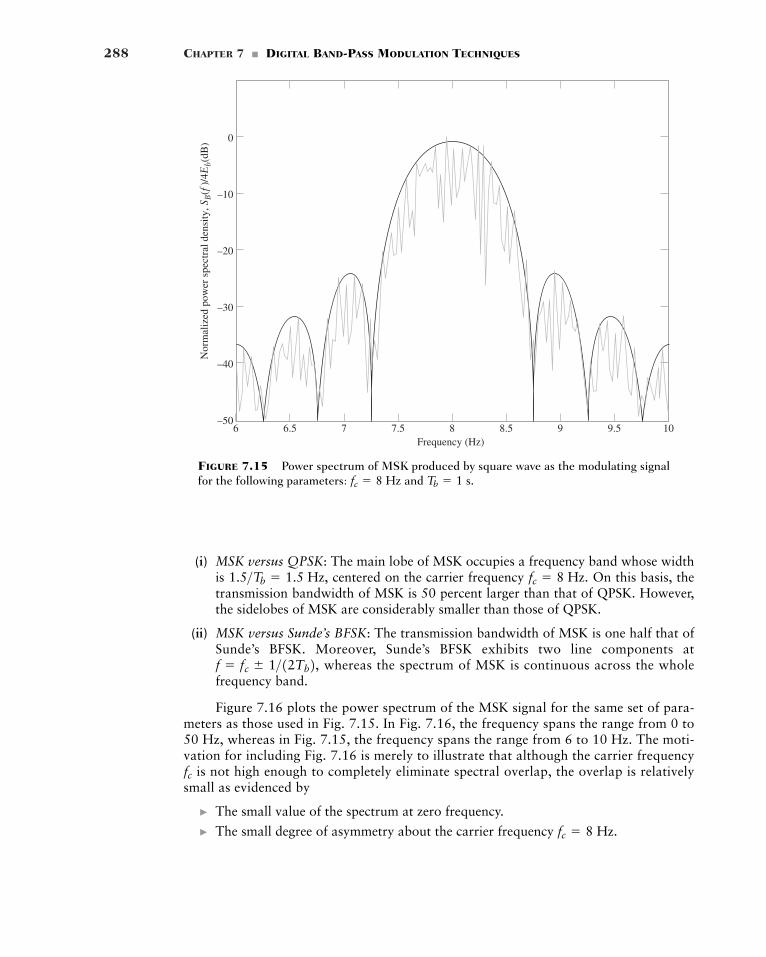
288 CHAPTER 7 � DIGITAL BAND-PASS MODULATION TECHNIQUES
6 6.5 7 7.5 8 8.5 9 9.5 10
Nor
mal
ized
pow
er s
pect
ral d
ensi
ty, S
B(f
)/4E
b(dB
)
–50
Frequency (Hz)
–30
–40
–20
–10
0
FIGURE 7.15 Power spectrum of MSK produced by square wave as the modulating signalfor the following parameters: and Tb � 1 s.fc � 8 Hz
(i) MSK versus QPSK: The main lobe of MSK occupies a frequency band whose widthis centered on the carrier frequency On this basis, thetransmission bandwidth of MSK is 50 percent larger than that of QPSK. However,the sidelobes of MSK are considerably smaller than those of QPSK.
(ii) MSK versus Sunde’s BFSK: The transmission bandwidth of MSK is one half that ofSunde’s BFSK. Moreover, Sunde’s BFSK exhibits two line components at
whereas the spectrum of MSK is continuous across the wholefrequency band.
Figure 7.16 plots the power spectrum of the MSK signal for the same set of para-meters as those used in Fig. 7.15. In Fig. 7.16, the frequency spans the range from 0 to50 Hz, whereas in Fig. 7.15, the frequency spans the range from 6 to 10 Hz. The moti-vation for including Fig. 7.16 is merely to illustrate that although the carrier frequency
is not high enough to completely eliminate spectral overlap, the overlap is relativelysmall as evidenced by
� The small value of the spectrum at zero frequency.
� The small degree of asymmetry about the carrier frequency fc � 8 Hz.
fc
f � fc � 1>12Tb2,
fc � 8 Hz.1.5>Tb � 1.5 Hz,
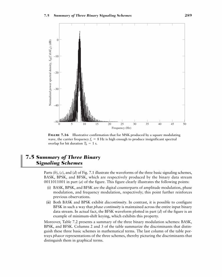
7.5 Summary of Three Binary Signaling Schemes 289
0 5 10 15 20 25 30 35 40 45 50
Nor
mal
ized
pow
er s
pect
ral d
ensi
ty, S
B(f
)/(4
Eb)
, (dB
)
–50
Frequency (Hz)
–30
–40
–20
–10
0
FIGURE 7.16 Illustrative confirmation that for MSK produced by a square modulatingwave, the carrier frequency is high enough to produce insignificant spectraloverlap for bit duration Tb � 1 s.
fc � 8 Hz
7.5 Summary of Three Binary Signaling Schemes
Parts (b), (c), and (d) of Fig. 7.1 illustrate the waveforms of the three basic signaling schemes,BASK, BPSK, and BFSK, which are respectively produced by the binary data stream0011011001 in part (a) of the figure. This figure clearly illustrates the following points:
(i) BASK, BPSK, and BFSK are the digital counterparts of amplitude modulation, phasemodulation, and frequency modulation, respectively; this point further reinforcesprevious observations.
(ii) Both BASK and BPSK exhibit discontinuity. In contrast, it is possible to configureBFSK in such a way that phase continuity is maintained across the entire input binarydata stream. In actual fact, the BFSK waveform plotted in part (d) of the figure is anexample of minimum-shift keying, which exhibits this property.
Moreover, Table 7.2 presents a summary of the three binary modulation schemes: BASK,BPSK, and BFSK. Columns 2 and 3 of the table summarize the discriminants that distin-guish these three basic schemes in mathematical terms. The last column of the table por-trays phasor representations of the three schemes, thereby picturing the discriminants thatdistinguish them in graphical terms.
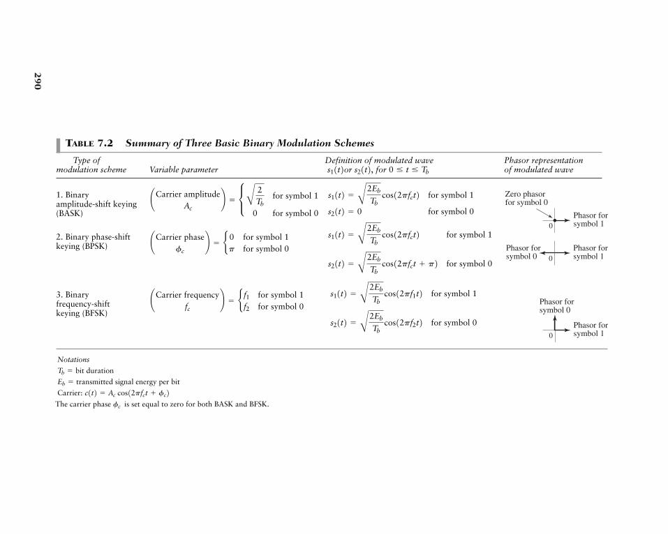
290
TABLE 7.2 Summary of Three Basic Binary Modulation Schemes
Type of Definition of modulated wave Phasor representationmodulation scheme Variable parameter or for of modulated wave0 � t � Tbs21t2,s11t21. Binary amplitude-shift keying(BASK)
2. Binary phase-shiftkeying (BPSK)
3. Binary frequency-shiftkeying (BFSK)
¢Carrier frequencyfc
≤ � b f1 for symbol 1f2 for symbol 0
¢Carrier phasefc
≤ � b 0 for symbol 1p for symbol 0
¢Carrier amplitudeAc
≤ � c B 2Tb
for symbol 1
0 for symbol 0
s21t2 � B2Eb
Tbcos12pf2t2 for symbol 0
s11t2 � B2Eb
Tbcos12pf1t2 for symbol 1
s21t2 � B2Eb
Tbcos12pfct p2 for symbol 0
s11t2 � B2Eb
Tbcos12pfct2 for symbol 1
s21t2 � 0 for symbol 0
s11t2 � B2Eb
Tbcos12pfct2 for symbol 1
0Phasor forsymbol 1
Phasor forsymbol 0
0Phasor forsymbol 1
Phasor forsymbol 0
0
Zero phasorfor symbol 0
Phasor forsymbol 1
Notations
Carrier:
The carrier phase is set equal to zero for both BASK and BFSK.fc
c1t2 � Ac cos12pfct fc2Eb � transmitted signal energy per bit
Tb � bit duration
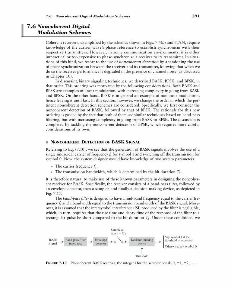
7.6 Noncoherent Digital Modulation Schemes 291
7.6 Noncoherent Digital Modulation Schemes
Coherent receivers, exemplified by the schemes shown in Figs. 7.4(b) and 7.7(b), requireknowledge of the carrier wave’s phase reference to establish synchronism with theirrespective transmitters. However, in some communication environments, it is eitherimpractical or too expensive to phase-synchronize a receiver to its transmitter. In situa-tions of this kind, we resort to the use of noncoherent detection by abandoning the useof phase synchronization between the receiver and its transmitter, knowing that when wedo so the receiver performance is degraded in the presence of channel noise (as discussedin Chapter 10).
In discussing binary signaling techniques, we described BASK, BPSK, and BFSK, inthat order. This ordering was motivated by the following considerations. Both BASK andBPSK are examples of linear modulation, with increasing complexity in going from BASKand BPSK. On the other hand, BFSK is in general an example of nonlinear modulation,hence leaving it until last. In this section, however, we change the order in which the per-tinent noncoherent detection schemes are considered. Specifically, we first consider thenoncoherent detection of BASK, followed by that of BFSK. The rationale for this newordering is guided by the fact that both of them use similar techniques based on band-passfiltering, but with increasing complexity in going from BASK to BFSK. The discussion iscompleted by tackling the noncoherent detection of BPSK, which requires more carefulconsiderations of its own.
� NONCOHERENT DETECTION OF BASK SIGNAL
Referring to Eq. (7.10), we see that the generation of BASK signals involves the use of asingle sinusoidal carrier of frequency for symbol 1 and switching off the transmission forsymbol 0. Now, the system designer would have knowledge of two system parameters:
� The carrier frequency � The transmission bandwidth, which is determined by the bit duration
It is therefore natural to make use of these known parameters in designing the noncoher-ent receiver for BASK. Specifically, the receiver consists of a band-pass filter, followed byan envelope detector, then a sampler, and finally a decision-making device, as depicted inFig. 7.17.
The band-pass filter is designed to have a mid-band frequency equal to the carrier fre-quency and a bandwidth equal to the transmission bandwidth of the BASK signal. More-over, it is assumed that the intersymbol interference (ISI) produced by the filter is negligible,which, in turn, requires that the rise time and decay time of the response of the filter to arectangular pulse be short compared to the bit duration Under these conditions, weTb .
fc
Tb .fc .
fc
Band-pass filter tuned to fc
Envelopedetector
Decision-makingdevice
Sample attime t = iTb
Say symbol 1 if thethreshold is exceeded
Otherwise, say symbol 0
BASKsignal
Threshold
FIGURE 7.17 Noncoherent BASK receiver; the integer i for the sampler equals 0, �1, �2, Á .
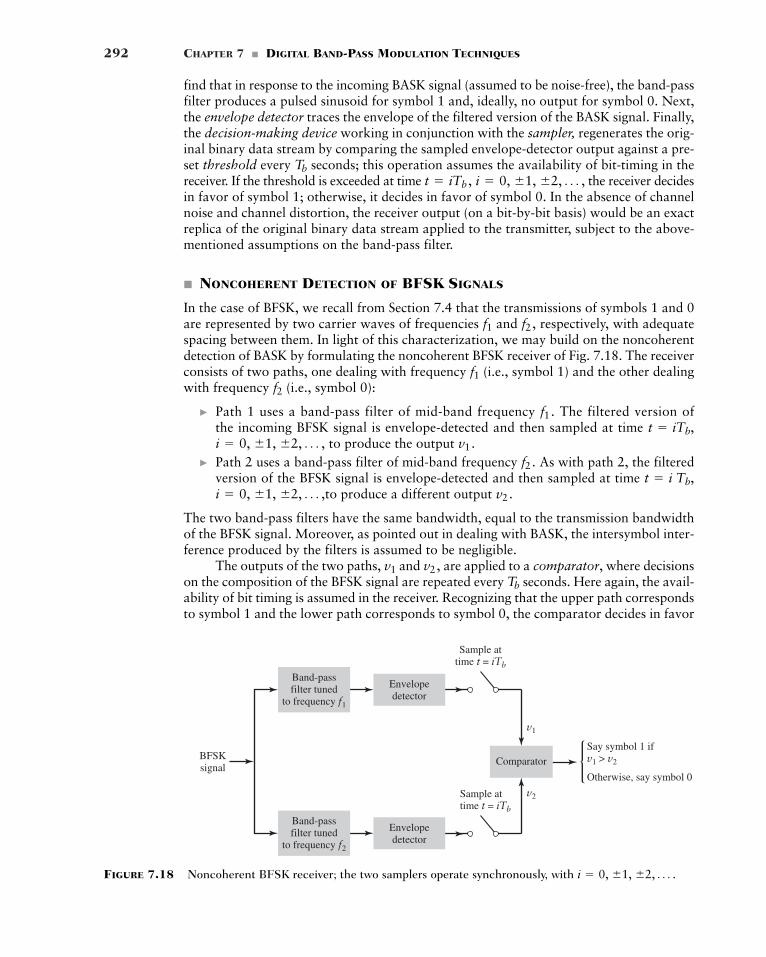
292 CHAPTER 7 � DIGITAL BAND-PASS MODULATION TECHNIQUES
Sample attime t = iTb
Sample attime t = iTb
Envelopedetector
Envelopedetector
Band-passfilter tuned
to frequency f2
Band-passfilter tuned
to frequency f1
Say symbol 1 ifv1 > v2
v1
v2
Otherwise, say symbol 0
BFSKsignal
Comparator
FIGURE 7.18 Noncoherent BFSK receiver; the two samplers operate synchronously, with i � 0, �1, �2, Á .
find that in response to the incoming BASK signal (assumed to be noise-free), the band-passfilter produces a pulsed sinusoid for symbol 1 and, ideally, no output for symbol 0. Next,the envelope detector traces the envelope of the filtered version of the BASK signal. Finally,the decision-making device working in conjunction with the sampler, regenerates the orig-inal binary data stream by comparing the sampled envelope-detector output against a pre-set threshold every seconds; this operation assumes the availability of bit-timing in thereceiver. If the threshold is exceeded at time the receiver decidesin favor of symbol 1; otherwise, it decides in favor of symbol 0. In the absence of channelnoise and channel distortion, the receiver output (on a bit-by-bit basis) would be an exactreplica of the original binary data stream applied to the transmitter, subject to the above-mentioned assumptions on the band-pass filter.
� NONCOHERENT DETECTION OF BFSK SIGNALS
In the case of BFSK, we recall from Section 7.4 that the transmissions of symbols 1 and 0are represented by two carrier waves of frequencies and respectively, with adequatespacing between them. In light of this characterization, we may build on the noncoherentdetection of BASK by formulating the noncoherent BFSK receiver of Fig. 7.18. The receiverconsists of two paths, one dealing with frequency (i.e., symbol 1) and the other dealingwith frequency (i.e., symbol 0):
� Path 1 uses a band-pass filter of mid-band frequency The filtered version ofthe incoming BFSK signal is envelope-detected and then sampled at time
to produce the output � Path 2 uses a band-pass filter of mid-band frequency As with path 2, the filtered
version of the BFSK signal is envelope-detected and then sampled at time to produce a different output
The two band-pass filters have the same bandwidth, equal to the transmission bandwidthof the BFSK signal. Moreover, as pointed out in dealing with BASK, the intersymbol inter-ference produced by the filters is assumed to be negligible.
The outputs of the two paths, and are applied to a comparator, where decisionson the composition of the BFSK signal are repeated every seconds. Here again, the avail-ability of bit timing is assumed in the receiver. Recognizing that the upper path correspondsto symbol 1 and the lower path corresponds to symbol 0, the comparator decides in favor
Tb
v2,v1
v2.i � 0, �1, �2, Á ,t � i Tb,
f2.v1.i � 0, �1, �2, Á ,
t � iTb,f1.
f2f1
f2,f1
t � iTb , i � 0, �1, �2, Á ,Tb
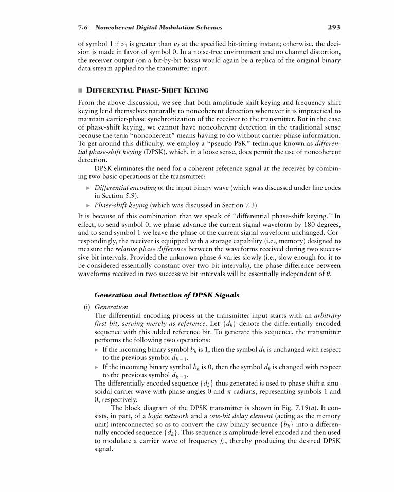
7.6 Noncoherent Digital Modulation Schemes 293
of symbol 1 if is greater than at the specified bit-timing instant; otherwise, the deci-sion is made in favor of symbol 0. In a noise-free environment and no channel distortion,the receiver output (on a bit-by-bit basis) would again be a replica of the original binarydata stream applied to the transmitter input.
� DIFFERENTIAL PHASE-SHIFT KEYING
From the above discussion, we see that both amplitude-shift keying and frequency-shiftkeying lend themselves naturally to noncoherent detection whenever it is impractical tomaintain carrier-phase synchronization of the receiver to the transmitter. But in the caseof phase-shift keying, we cannot have noncoherent detection in the traditional sensebecause the term “noncoherent” means having to do without carrier-phase information.To get around this difficulty, we employ a “pseudo PSK” technique known as differen-tial phase-shift keying (DPSK), which, in a loose sense, does permit the use of noncoherentdetection.
DPSK eliminates the need for a coherent reference signal at the receiver by combin-ing two basic operations at the transmitter:
� Differential encoding of the input binary wave (which was discussed under line codesin Section 5.9).
� Phase-shift keying (which was discussed in Section 7.3).
It is because of this combination that we speak of “differential phase-shift keying.” Ineffect, to send symbol 0, we phase advance the current signal waveform by 180 degrees,and to send symbol 1 we leave the phase of the current signal waveform unchanged. Cor-respondingly, the receiver is equipped with a storage capability (i.e., memory) designed tomeasure the relative phase difference between the waveforms received during two succes-sive bit intervals. Provided the unknown phase varies slowly (i.e., slow enough for it tobe considered essentially constant over two bit intervals), the phase difference betweenwaveforms received in two successive bit intervals will be essentially independent of
Generation and Detection of DPSK Signals
(i) GenerationThe differential encoding process at the transmitter input starts with an arbitraryfirst bit, serving merely as reference. Let denote the differentially encodedsequence with this added reference bit. To generate this sequence, the transmitterperforms the following two operations:� If the incoming binary symbol is 1, then the symbol is unchanged with respect
to the previous symbol .� If the incoming binary symbol is 0, then the symbol is changed with respect
to the previous symbol .The differentially encoded sequence thus generated is used to phase-shift a sinu-soidal carrier wave with phase angles 0 and radians, representing symbols 1 and0, respectively.
The block diagram of the DPSK transmitter is shown in Fig. 7.19(a). It con-sists, in part, of a logic network and a one-bit delay element (acting as the memoryunit) interconnected so as to convert the raw binary sequence into a differen-tially encoded sequence This sequence is amplitude-level encoded and then usedto modulate a carrier wave of frequency thereby producing the desired DPSKsignal.
fc ,5dk6. 5bk6
p
5dk6dk�1
dkbk
dk�1
dkbk
5dk6
u.
u
v2v1
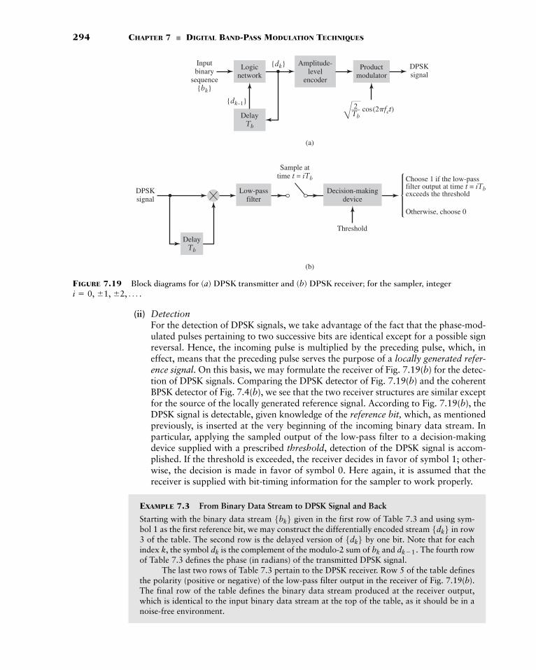
294 CHAPTER 7 � DIGITAL BAND-PASS MODULATION TECHNIQUES
(a)
Logicnetwork
DelayTb
Amplitude-level
encoder
Productmodulator
Inputbinary
sequence{bk}
{dk–1}
{dk} DPSKsignal
D2
Tbcos(2�fct)—
(b)
DelayTb
Low-passfilter
DPSKsignal
Decision-makingdevice
Sample attime t = iTb Choose 1 if the low-pass
filter output at time t = iTbexceeds the threshold
Otherwise, choose 0
Threshold
FIGURE 7.19 Block diagrams for (a) DPSK transmitter and (b) DPSK receiver; for the sampler, integeri � 0, �1, �2, Á .
(ii) DetectionFor the detection of DPSK signals, we take advantage of the fact that the phase-mod-ulated pulses pertaining to two successive bits are identical except for a possible signreversal. Hence, the incoming pulse is multiplied by the preceding pulse, which, ineffect, means that the preceding pulse serves the purpose of a locally generated refer-ence signal. On this basis, we may formulate the receiver of Fig. 7.19(b) for the detec-tion of DPSK signals. Comparing the DPSK detector of Fig. 7.19(b) and the coherentBPSK detector of Fig. 7.4(b), we see that the two receiver structures are similar exceptfor the source of the locally generated reference signal. According to Fig. 7.19(b), theDPSK signal is detectable, given knowledge of the reference bit, which, as mentionedpreviously, is inserted at the very beginning of the incoming binary data stream. Inparticular, applying the sampled output of the low-pass filter to a decision-makingdevice supplied with a prescribed threshold, detection of the DPSK signal is accom-plished. If the threshold is exceeded, the receiver decides in favor of symbol 1; other-wise, the decision is made in favor of symbol 0. Here again, it is assumed that thereceiver is supplied with bit-timing information for the sampler to work properly.
EXAMPLE 7.3 From Binary Data Stream to DPSK Signal and Back
Starting with the binary data stream given in the first row of Table 7.3 and using sym-bol 1 as the first reference bit, we may construct the differentially encoded stream in row3 of the table. The second row is the delayed version of by one bit. Note that for eachindex k, the symbol is the complement of the modulo-2 sum of and The fourth rowof Table 7.3 defines the phase (in radians) of the transmitted DPSK signal.
The last two rows of Table 7.3 pertain to the DPSK receiver. Row 5 of the table definesthe polarity (positive or negative) of the low-pass filter output in the receiver of Fig. 7.19(b).The final row of the table defines the binary data stream produced at the receiver output,which is identical to the input binary data stream at the top of the table, as it should be in anoise-free environment.
dk�1.bkdk
5dk6 5dk65bk6
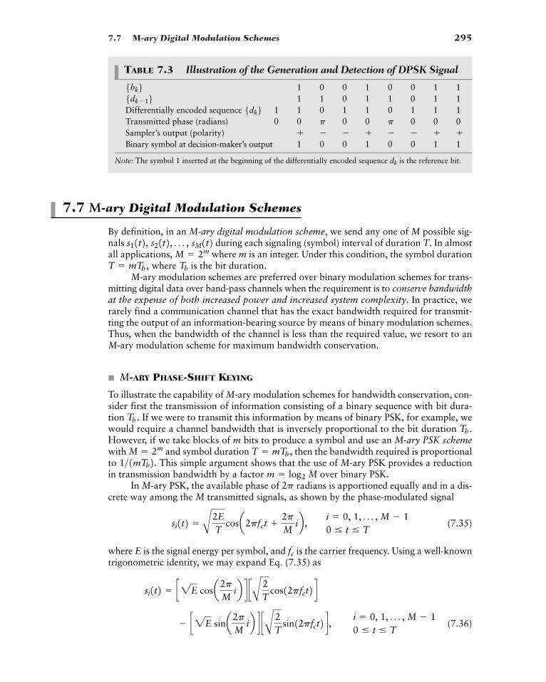
7.7 M-ary Digital Modulation Schemes 295
7.7 M-ary Digital Modulation Schemes
By definition, in an M-ary digital modulation scheme, we send any one of M possible sig-nals during each signaling (symbol) interval of duration T. In almostall applications, where m is an integer. Under this condition, the symbol duration
where is the bit duration.M-ary modulation schemes are preferred over binary modulation schemes for trans-
mitting digital data over band-pass channels when the requirement is to conserve bandwidthat the expense of both increased power and increased system complexity. In practice, werarely find a communication channel that has the exact bandwidth required for transmit-ting the output of an information-bearing source by means of binary modulation schemes.Thus, when the bandwidth of the channel is less than the required value, we resort to anM-ary modulation scheme for maximum bandwidth conservation.
� M-ARY PHASE-SHIFT KEYING
To illustrate the capability of M-ary modulation schemes for bandwidth conservation, con-sider first the transmission of information consisting of a binary sequence with bit dura-tion If we were to transmit this information by means of binary PSK, for example, wewould require a channel bandwidth that is inversely proportional to the bit duration However, if we take blocks of m bits to produce a symbol and use an M-ary PSK schemewith and symbol duration then the bandwidth required is proportionalto This simple argument shows that the use of M-ary PSK provides a reductionin transmission bandwidth by a factor over binary PSK.
In M-ary PSK, the available phase of radians is apportioned equally and in a dis-crete way among the M transmitted signals, as shown by the phase-modulated signal
(7.35)
where E is the signal energy per symbol, and is the carrier frequency. Using a well-knowntrigonometric identity, we may expand Eq. (7.35) as
(7.36)� c2E sina2pM
ib d cA 2T
sin12pfct2 d , i � 0, 1, Á , M � 10 � t � T
si1t2 � c2E cosa2pM
ib d cA 2T
cos12pfct2 d
fc
si1t2 � A2ET
cosa2pfct 2pM
ib , i � 0, 1, Á , M � 10 � t � T
2pm � log2 M
1>1mTb2. T � mTb ,M � 2m
Tb .Tb .
TbT � mTb ,M � 2m
s11t2, s21t2, Á , sM1t2
TABLE 7.3 Illustration of the Generation and Detection of DPSK Signal
1 0 0 1 0 0 1 11 1 0 1 1 0 1 1
Differentially encoded sequence 1 1 0 1 1 0 1 1 1Transmitted phase (radians) 0 0 0 0 0 0 0Sampler’s output (polarity)Binary symbol at decision-maker’s output 1 0 0 1 0 0 1 1
Note: The symbol 1 inserted at the beginning of the differentially encoded sequence is the reference bit.dk
����
pp
5dk65dk�165bk6
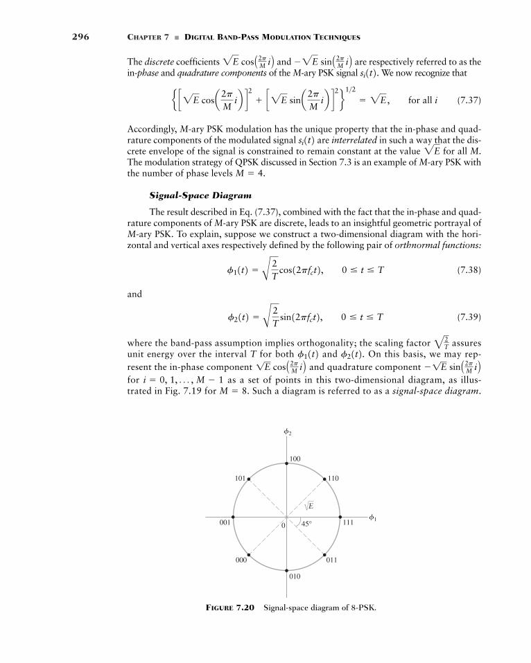
296 CHAPTER 7 � DIGITAL BAND-PASS MODULATION TECHNIQUES
The discrete coefficients and are respectively referred to as thein-phase and quadrature components of the M-ary PSK signal We now recognize that
(7.37)
Accordingly, M-ary PSK modulation has the unique property that the in-phase and quad-rature components of the modulated signal are interrelated in such a way that the dis-crete envelope of the signal is constrained to remain constant at the value for all M.The modulation strategy of QPSK discussed in Section 7.3 is an example of M-ary PSK withthe number of phase levels
Signal-Space Diagram
The result described in Eq. (7.37), combined with the fact that the in-phase and quad-rature components of M-ary PSK are discrete, leads to an insightful geometric portrayal ofM-ary PSK. To explain, suppose we construct a two-dimensional diagram with the hori-zontal and vertical axes respectively defined by the following pair of orthnormal functions:
(7.38)
and
(7.39)
where the band-pass assumption implies orthogonality; the scaling factor assuresunit energy over the interval T for both and On this basis, we may rep-resent the in-phase component and quadrature componentfor as a set of points in this two-dimensional diagram, as illus-trated in Fig. 7.19 for Such a diagram is referred to as a signal-space diagram.M � 8.
i � 0, 1, Á , M � 1�1E sin A2pM i B1E cos A2pM i B f21t2.f11t2 22
T
f21t2 � A 2T
sin12pfct2, 0 � t � T
f11t2 � A 2T
cos12pfct2, 0 � t � T
M � 4.
2Esi1t2
e c2E cosa2pM
ib d2 c2E sina2pM
ib d2 f1>2� 2E , for all i
si1t2.�2E sin A2pM i B2E cos A2pM i B
100
110
�2
�1111
011
101
001
000
0 45°
010
/E
FIGURE 7.20 Signal-space diagram of 8-PSK.
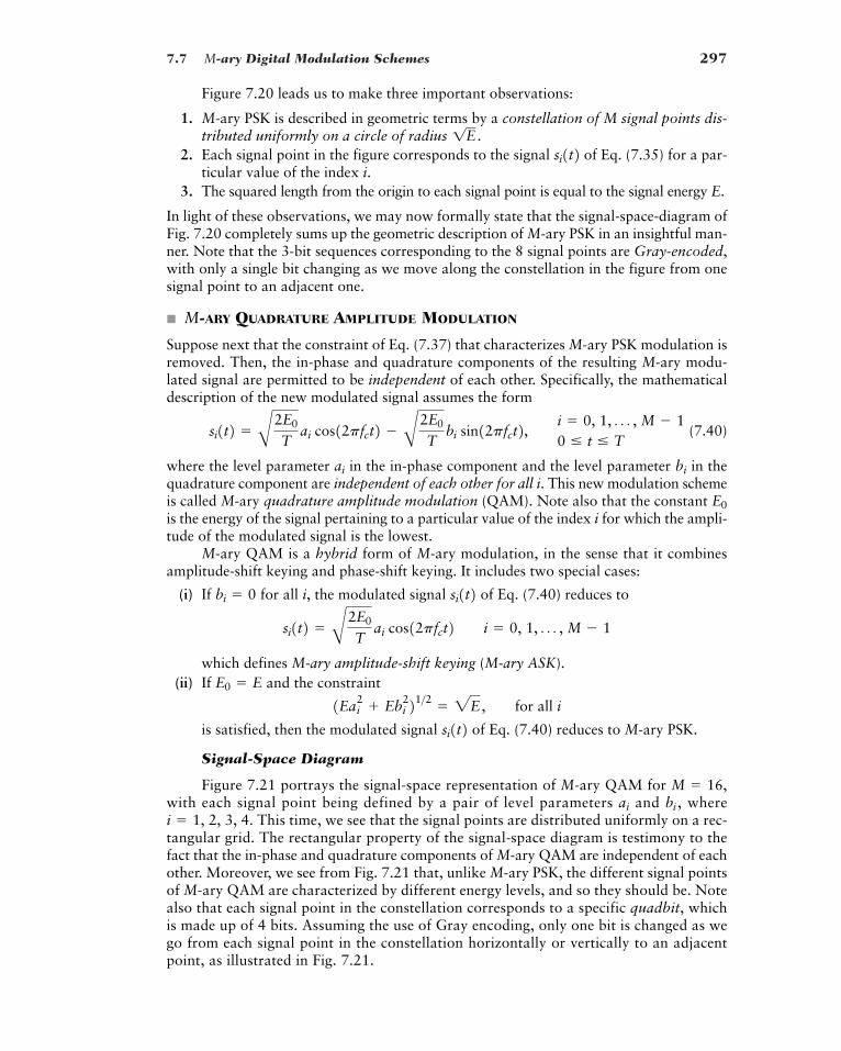
7.7 M-ary Digital Modulation Schemes 297
Figure 7.20 leads us to make three important observations:
1. M-ary PSK is described in geometric terms by a constellation of M signal points dis-tributed uniformly on a circle of radius
2. Each signal point in the figure corresponds to the signal of Eq. (7.35) for a par-ticular value of the index i.
3. The squared length from the origin to each signal point is equal to the signal energy E.
In light of these observations, we may now formally state that the signal-space-diagram ofFig. 7.20 completely sums up the geometric description of M-ary PSK in an insightful man-ner. Note that the 3-bit sequences corresponding to the 8 signal points are Gray-encoded,with only a single bit changing as we move along the constellation in the figure from onesignal point to an adjacent one.
� M-ARY QUADRATURE AMPLITUDE MODULATION
Suppose next that the constraint of Eq. (7.37) that characterizes M-ary PSK modulation isremoved. Then, the in-phase and quadrature components of the resulting M-ary modu-lated signal are permitted to be independent of each other. Specifically, the mathematicaldescription of the new modulated signal assumes the form
(7.40)
where the level parameter in the in-phase component and the level parameter in thequadrature component are independent of each other for all i. This new modulation schemeis called M-ary quadrature amplitude modulation (QAM). Note also that the constant is the energy of the signal pertaining to a particular value of the index i for which the ampli-tude of the modulated signal is the lowest.
M-ary QAM is a hybrid form of M-ary modulation, in the sense that it combinesamplitude-shift keying and phase-shift keying. It includes two special cases:
(i) If for all i, the modulated signal of Eq. (7.40) reduces to
which defines M-ary amplitude-shift keying (M-ary ASK).(ii) If and the constraint
is satisfied, then the modulated signal of Eq. (7.40) reduces to M-ary PSK.
Signal-Space Diagram
Figure 7.21 portrays the signal-space representation of M-ary QAM for with each signal point being defined by a pair of level parameters and where
This time, we see that the signal points are distributed uniformly on a rec-tangular grid. The rectangular property of the signal-space diagram is testimony to thefact that the in-phase and quadrature components of M-ary QAM are independent of eachother. Moreover, we see from Fig. 7.21 that, unlike M-ary PSK, the different signal pointsof M-ary QAM are characterized by different energy levels, and so they should be. Notealso that each signal point in the constellation corresponds to a specific quadbit, whichis made up of 4 bits. Assuming the use of Gray encoding, only one bit is changed as wego from each signal point in the constellation horizontally or vertically to an adjacentpoint, as illustrated in Fig. 7.21.
i � 1, 2, 3, 4.bi ,ai
M � 16,
si1t21Eai
2 Ebi
221>2 � 2E , for all i
E0 � E
si1t2 � B2E0
Tai cos12pfct2 i � 0, 1, Á , M � 1
si1t2bi � 0
E0
biai
si1t2 � B2E0
Tai cos12pfct2 � B2E0
Tbi sin12pfct2, i � 0, 1, Á , M � 1
0 � t � T
si1t21E .
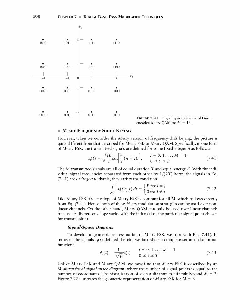
298 CHAPTER 7 � DIGITAL BAND-PASS MODULATION TECHNIQUES
� M-ARY FREQUENCY-SHIFT KEYING
However, when we consider the M-ary version of frequency-shift keying, the picture isquite different from that described for M-ary PSK or M-ary QAM. Specifically, in one formof M-ary FSK, the transmitted signals are defined for some fixed integer n as follows:
(7.41)
The M transmitted signals are all of equal duration T and equal energy E. With the indi-vidual signal frequencies separated from each other by hertz, the signals in Eq.(7.41) are orthogonal; that is, they satisfy the condition
(7.42)
Like M-ary PSK, the envelope of M-ary FSK is constant for all M, which follows directlyfrom Eq. (7.41). Hence, both of these M-ary modulation strategies can be used over non-linear channels. On the other hand, M-ary QAM can only be used over linear channelsbecause its discrete envelope varies with the index i (i.e., the particular signal point chosenfor transmission).
Signal-Space Diagram
To develop a geometric representation of M-ary FSK, we start with Eq. (7.41). Interms of the signals defined therein, we introduce a complete set of orthonormalfunctions:
(7.43)
Unlike M-ary PSK and M-ary QAM, we now find that M-ary FSK is described by anM-dimensional signal-space diagram, where the number of signal points is equal to thenumber of coordinates. The visualization of such a diagram is difficult beyond Figure 7.22 illustrates the geometric representation of M-ary FSK for M � 3.
M � 3.
fi1t2 �1
2Esi1t2 i � 0, 1, Á , M � 1
0 � t � T
si1t2
LT
0si1t2sj1t2 dt � bE for i � j
0 for i j
1>12T2si1t2 � A2E
Tcos cp
T1n i2t d , i � 0, 1, Á , M � 1
0 � t � T
�2
�1
1110111110111010
1100110110011000
0100010100010000
0110011100110010
–3 3–1 10
–1
1
3
–3
FIGURE 7.21 Signal-space diagram of Gray-encoded M-ary QAM for M � 16.
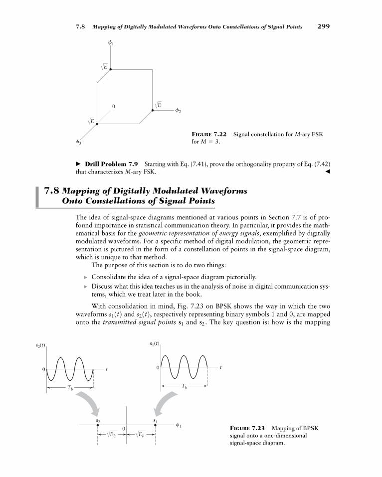
7.8 Mapping of Digitally Modulated Waveforms Onto Constellations of Signal Points 299
�20
�3
�1
/E/E
/E
FIGURE 7.22 Signal constellation for M-ary FSKfor M � 3.
�1
t
s2
Tb
s2(t)
0
0
s1
t
Tb
s1(t)
0
/Eb /Eb
FIGURE 7.23 Mapping of BPSKsignal onto a one-dimensional signal-space diagram.
� Drill Problem 7.9 Starting with Eq. (7.41), prove the orthogonality property of Eq. (7.42)that characterizes M-ary FSK. �
7.8 Mapping of Digitally Modulated WaveformsOnto Constellations of Signal Points
The idea of signal-space diagrams mentioned at various points in Section 7.7 is of pro-found importance in statistical communication theory. In particular, it provides the math-ematical basis for the geometric representation of energy signals, exemplified by digitallymodulated waveforms. For a specific method of digital modulation, the geometric repre-sentation is pictured in the form of a constellation of points in the signal-space diagram,which is unique to that method.
The purpose of this section is to do two things:
� Consolidate the idea of a signal-space diagram pictorially.� Discuss what this idea teaches us in the analysis of noise in digital communication sys-
tems, which we treat later in the book.
With consolidation in mind, Fig. 7.23 on BPSK shows the way in which the twowaveforms and respectively representing binary symbols 1 and 0, are mappedonto the transmitted signal points and The key question is: how is the mappings2.s1
s21t2,s11t2
300 CHAPTER 7 � DIGITAL BAND-PASS MODULATION TECHNIQUES
accomplished? The answer lies in the use of a correlator. First, we note that the signal-space representation of BPSK is simple, involving a single basis function:
(7.44)
In more specific terms, each of the two signaling waveforms and is correlatedwith the basis function The use of correlation provides another way of designing areceiver for the coherent detection of BPSK. For the issue at hand, we proceed in two stepsas follows:
1. Correlating the signal
(7.45)
with the basis function over the time interval we get the signalpoint
(7.46)
Under the band-pass assumption, Eq. (7.46) simplifies to
(7.47)2. Similarly, we may show that the signal
(7.48)
is represented by the signal point
(7.49)
These two results are indeed what is portrayed in Fig. 7.23.
� Drill Problem 7.10 Justify Eqs. (7.47) and (7.49). �
Consider next the picture depicted in Fig. 7.24, pertaining to BFSK. As with BPSK, thesignal-space diagram consists of two transmitted signal points: the point representing thetransmission of binary symbol 1 and the point representing the transmission of binarysymbol 0. Following a procedure similar to that which led to the signal-space mapping ofBPSK, we may construct the signal-space mapping of Fig. 7.24 for BFSK, where the twosignal points are defined by
(7.50)
and
(7.51)
The two signal-space diagrams of Figs. 7.23 and 7.24 differ in one important respect:dimensionality, which is defined by the pertinent number of basis functions. The BPSK sig-
s2 � B 02EbR
s1 � B2Eb
0R
s2
s1
s2 � �2Eb
s21t2 � �B2Eb
Tb cos12pfct2 for symbol 0
s1 � 2Eb
� LT
b
0
2Tb2Eb cos212pfct2 dt
s1 � LT
b
0f11t2s11t2 dt
0 � t � Tb ,f11t2s11t2 � B2Eb
Tb cos12pfct2 for symbol 1
f11t2. s21t2s11t2f11t2 � B 2
Tb cos12pfct2
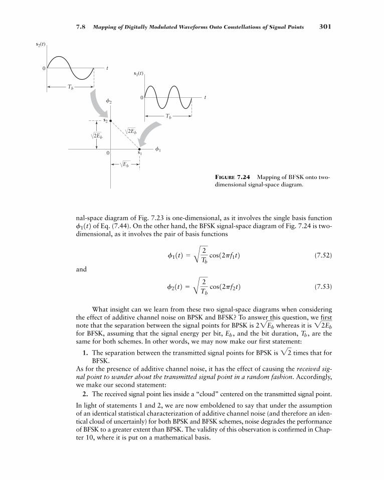
7.8 Mapping of Digitally Modulated Waveforms Onto Constellations of Signal Points 301
�1
�2
s2
0 s1
/Eb
/2Eb/2Eb
t
Tb
s1(t)
0
t
Tb
s2(t)
0
FIGURE 7.24 Mapping of BFSK onto two-dimensional signal-space diagram.
nal-space diagram of Fig. 7.23 is one-dimensional, as it involves the single basis functionof Eq. (7.44). On the other hand, the BFSK signal-space diagram of Fig. 7.24 is two-
dimensional, as it involves the pair of basis functions
(7.52)
and
(7.53)
What insight can we learn from these two signal-space diagrams when consideringthe effect of additive channel noise on BPSK and BFSK? To answer this question, we firstnote that the separation between the signal points for BPSK is whereas it is for BFSK, assuming that the signal energy per bit, and the bit duration, are thesame for both schemes. In other words, we may now make our first statement:
1. The separation between the transmitted signal points for BPSK is times that forBFSK.
As for the presence of additive channel noise, it has the effect of causing the received sig-nal point to wander about the transmitted signal point in a random fashion. Accordingly,we make our second statement:
2. The received signal point lies inside a “cloud” centered on the transmitted signal point.
In light of statements 1 and 2, we are now emboldened to say that under the assumptionof an identical statistical characterization of additive channel noise (and therefore an iden-tical cloud of uncertainly) for both BPSK and BFSK schemes, noise degrades the performanceof BFSK to a greater extent than BPSK. The validity of this observation is confirmed in Chap-ter 10, where it is put on a mathematical basis.
22
Tb ,Eb ,22Eb22Eb
f21t2 � B 2Tb
cos12pf2t2
f11t2 � B 2Tb
cos12pf1t2
f11t2
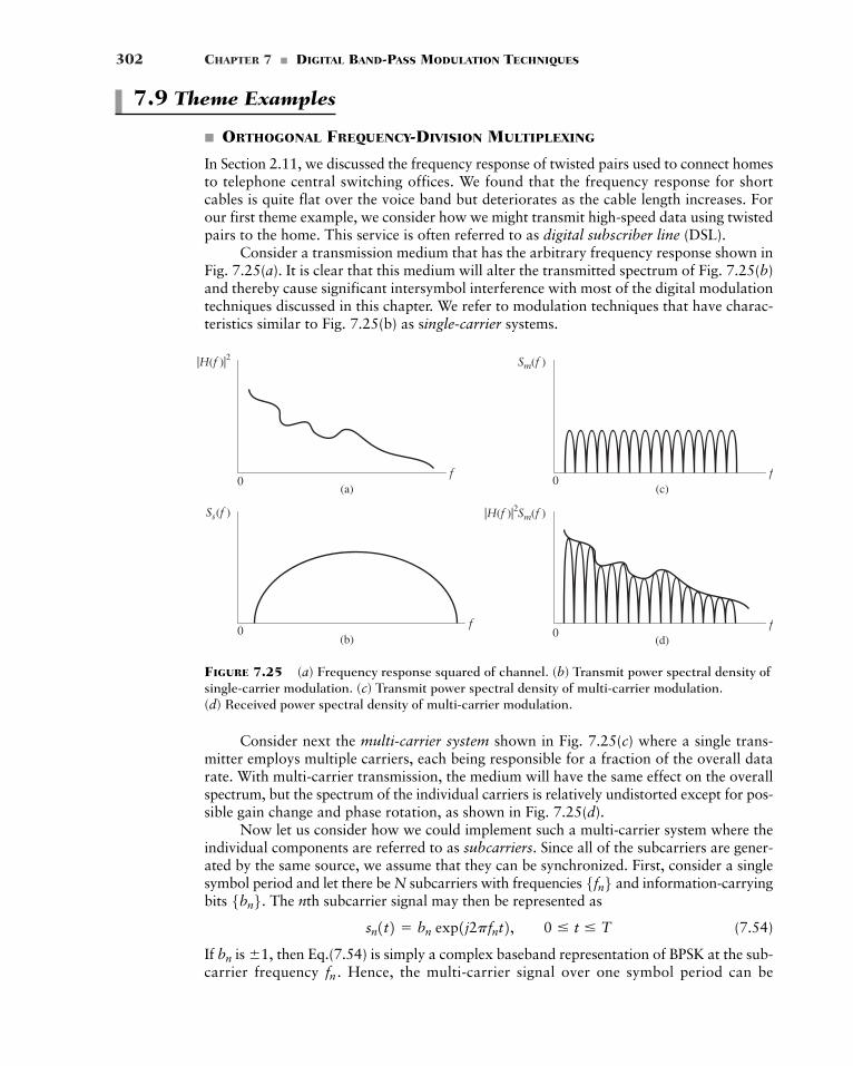
302 CHAPTER 7 � DIGITAL BAND-PASS MODULATION TECHNIQUES
f
|H(f )|2
f
Ss(f )
f
|H(f )|2Sm(f )
f
Sm(f )
(a)0
0 0
0
(b)
(c)
(d)
FIGURE 7.25 (a) Frequency response squared of channel. (b) Transmit power spectral density ofsingle-carrier modulation. (c) Transmit power spectral density of multi-carrier modulation. (d) Received power spectral density of multi-carrier modulation.
7.9 Theme Examples
� ORTHOGONAL FREQUENCY-DIVISION MULTIPLEXING
In Section 2.11, we discussed the frequency response of twisted pairs used to connect homesto telephone central switching offices. We found that the frequency response for shortcables is quite flat over the voice band but deteriorates as the cable length increases. Forour first theme example, we consider how we might transmit high-speed data using twistedpairs to the home. This service is often referred to as digital subscriber line (DSL).
Consider a transmission medium that has the arbitrary frequency response shown inFig. 7.25(a). It is clear that this medium will alter the transmitted spectrum of Fig. 7.25(b)and thereby cause significant intersymbol interference with most of the digital modulationtechniques discussed in this chapter. We refer to modulation techniques that have charac-teristics similar to Fig. 7.25(b) as single-carrier systems.
Consider next the multi-carrier system shown in Fig. 7.25(c) where a single trans-mitter employs multiple carriers, each being responsible for a fraction of the overall datarate. With multi-carrier transmission, the medium will have the same effect on the overallspectrum, but the spectrum of the individual carriers is relatively undistorted except for pos-sible gain change and phase rotation, as shown in Fig. 7.25(d).
Now let us consider how we could implement such a multi-carrier system where theindividual components are referred to as subcarriers. Since all of the subcarriers are gener-ated by the same source, we assume that they can be synchronized. First, consider a singlesymbol period and let there be N subcarriers with frequencies and information-carryingbits The nth subcarrier signal may then be represented as
(7.54)
If is then Eq.(7.54) is simply a complex baseband representation of BPSK at the sub-carrier frequency Hence, the multi-carrier signal over one symbol period can befn .
�1,bn
sn1t2 � bn exp1j2pfnt2, 0 � t � T
5bn6. 5fn6
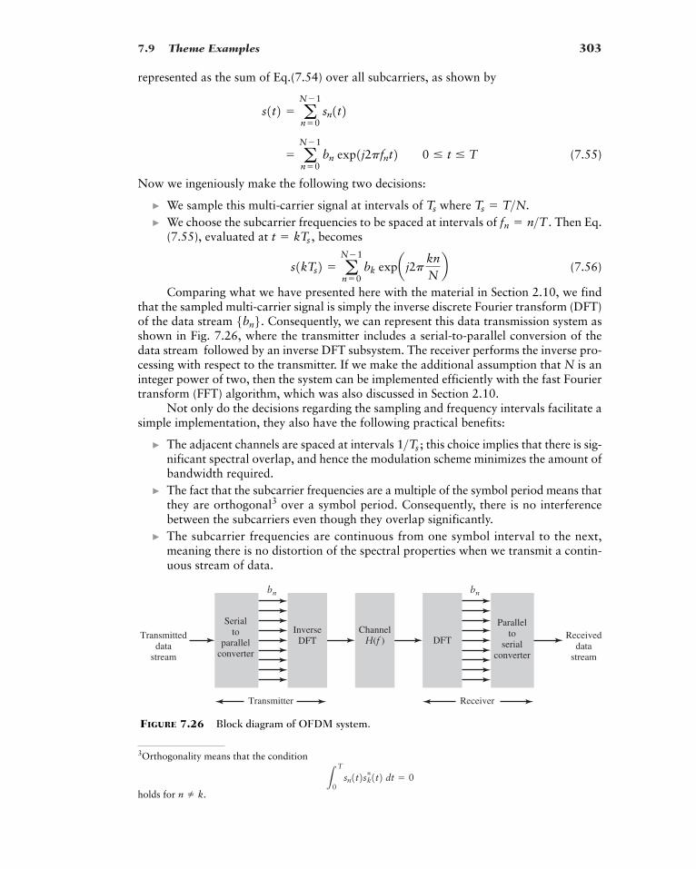
7.9 Theme Examples 303
represented as the sum of Eq.(7.54) over all subcarriers, as shown by
(7.55)
Now we ingeniously make the following two decisions:
� We sample this multi-carrier signal at intervals of where � We choose the subcarrier frequencies to be spaced at intervals of Then Eq.
(7.55), evaluated at becomes
(7.56)
Comparing what we have presented here with the material in Section 2.10, we findthat the sampled multi-carrier signal is simply the inverse discrete Fourier transform (DFT)of the data stream Consequently, we can represent this data transmission system asshown in Fig. 7.26, where the transmitter includes a serial-to-parallel conversion of thedata stream followed by an inverse DFT subsystem. The receiver performs the inverse pro-cessing with respect to the transmitter. If we make the additional assumption that N is aninteger power of two, then the system can be implemented efficiently with the fast Fouriertransform (FFT) algorithm, which was also discussed in Section 2.10.
Not only do the decisions regarding the sampling and frequency intervals facilitate asimple implementation, they also have the following practical benefits:
� The adjacent channels are spaced at intervals this choice implies that there is sig-nificant spectral overlap, and hence the modulation scheme minimizes the amount ofbandwidth required.
� The fact that the subcarrier frequencies are a multiple of the symbol period means thatthey are orthogonal3 over a symbol period. Consequently, there is no interferencebetween the subcarriers even though they overlap significantly.
� The subcarrier frequencies are continuous from one symbol interval to the next,meaning there is no distortion of the spectral properties when we transmit a contin-uous stream of data.
1>Ts ;
5bn6.
s1kTs2 � aN�1
n�0bk expa j2p kn
Nb
t � kTs ,fn � n>T .
Ts � T>N.Ts
� aN�1
n�0bn exp1j2pfnt2 0 � t � T
s1t2 � aN�1
n�0sn1t2
Parallelto
serialconverter
Transmitteddata
stream
Transmitter
Receiveddata
stream
Serialto
parallelconverter
InverseDFT
Receiver
ChannelH(f )
bn bn
DFT
FIGURE 7.26 Block diagram of OFDM system.
3Orthogonality means that the condition
holds for n k.L
T
0sn1t2sk
…1t2 dt � 0
304 CHAPTER 7 � DIGITAL BAND-PASS MODULATION TECHNIQUES
� Symbols may be continuously extended by a simple repetition referred to as cyclic pre-fix or postfix; this feature can be used beneficially in channels that tend to lengthenthe pulse interval.
The combination of the multiplexing subcarriers in the frequency domain and the orthog-onality of these subcarriers lead to the name orthogonal frequency division multiplex(OFDM) for this multi-carrier modulation technique.4
� GLOBAL SYSTEM FOR MOBILE (GSM) COMMUNICATION
In Chapter 4, we discussed the idea of frequency modulation, based on the definition
(7.57)
where the message signal is an analog signal. In this second theme example, we con-sider angle modulation that is produced by a digital message signal defined by
(7.58)
where T is the symbol period, is the data symbol of the nth symbol period, and is thepulse shape applied at each symbol period. In the historical course of events, analog modula-tion was the mainstay of radio communications for many years before the advent of digital com-munications. Consequently, for initial digital communications, it was often most convenientto use an FM transmitter, hence the term digital FM. Digital FM systems have a number ofadvantages, not the least of which is power efficiency due to their constant envelope.
The desirable power efficiency made digital FM a strong contender for wireless appli-cations using handheld terminals with small battery packs. In fact, a form of digital FM waschosen as a European standard in 1991 and later spread to other parts of the world underthe name GSM (Global System for Mobile Communications).
The actual modulation selected for GSM is called Gaussian minimum shift keying(GMSK), which is a special combination of Eqs. (7.57) and (7.58). In particular, we intro-duce three conditions:
1. The pulse shape is chosen to have the Gaussian shape
(7.59)
where the scale factor and the logarithm is the natural logarithm.2. The factor B controls the signal bandwidth, which, for prescribed symbol period T,
is chosen such that the time-bandwidth product 3. The frequency sensitivity factor of the modulator is selected such that the phase
change over one symbol period is radians.
Under these three conditions, it turns out that the resulting GMSK signal has a compactspectrum and may be coherently detected with only 0.46-dB degradation relative to idealBPSK performance in noise.
GSM communication (embodying GMSK) may therefore be viewed as a practicalexample of the evolution of an analog FM system to a digital system, which attempts toretain the advantages of the former.5
p>2kf
BT � 0.3.
c � B42p>log122,p1t2 � c exp5�pc2t26
p1t2bn
m1t2 � aN
n�0bnp1t � nT2
m1t2s1t2 � Ac cosa2pfct 2pkfL
t
0m1t2 dtb
5For detailed discussion of GMSK, see Steele and Hanzo (1999).
4For a more detailed discussion of OFDM, see Bahai and Saltzberg (1999).
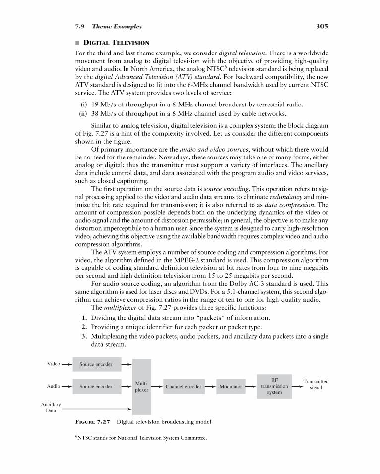
7.9 Theme Examples 305
Source encoder
Source encoderMulti-plexer
Channel encoder ModulatorRF
transmissionsystem
Video
Audio
AncillaryData
Transmittedsignal
FIGURE 7.27 Digital television broadcasting model.
� DIGITAL TELEVISION
For the third and last theme example, we consider digital television. There is a worldwidemovement from analog to digital television with the objective of providing high-qualityvideo and audio. In North America, the analog NTSC6 television standard is being replacedby the digital Advanced Television (ATV) standard. For backward compatibility, the newATV standard is designed to fit into the 6-MHz channel bandwidth used by current NTSCservice. The ATV system provides two levels of service:
(i) of throughput in a 6-MHz channel broadcast by terrestrial radio.(ii) of throughput in a 6 MHz channel used by cable networks.
Similar to analog television, digital television is a complex system; the block diagramof Fig. 7.27 is a hint of the complexity involved. Let us consider the different componentsshown in the figure.
Of primary importance are the audio and video sources, without which there wouldbe no need for the remainder. Nowadays, these sources may take one of many forms, eitheranalog or digital; thus the transmitter must support a variety of interfaces. The ancillarydata include control data, and data associated with the program audio and video services,such as closed captioning.
The first operation on the source data is source encoding. This operation refers to sig-nal processing applied to the video and audio data streams to eliminate redundancy and min-imize the bit rate required for transmission; it is also referred to as data compression. Theamount of compression possible depends both on the underlying dynamics of the video oraudio signal and the amount of distorsion permissible; in general, the objective is to make anydistortion imperceptibile to a human user. Since the system is designed to carry high-resolutionvideo, achieving this objective using the available bandwidth requires complex video and audiocompression algorithms.
The ATV system employs a number of source coding and compression algorithms. Forvideo, the algorithm defined in the MPEG-2 standard is used. This compression algorithmis capable of coding standard definition television at bit rates from four to nine megabitsper second and high definition television from 15 to 25 megabits per second.
For audio source coding, an algorithm from the Dolby AC-3 standard is used. Thissame algorithm is used for laser discs and DVDs. For a 5.1-channel system, this second algo-rithm can achieve compression ratios in the range of ten to one for high-quality audio.
The multiplexer of Fig. 7.27 provides three specific functions:
1. Dividing the digital data stream into “packets” of information.2. Providing a unique identifier for each packet or packet type.3. Multiplexing the video packets, audio packets, and ancillary data packets into a single
data stream.
38 Mb>s19 Mb>s
6NTSC stands for National Television System Committee.
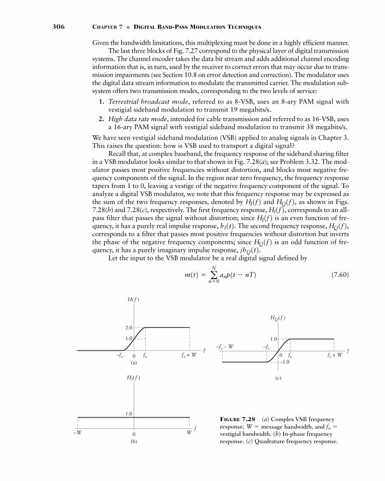
306 CHAPTER 7 � DIGITAL BAND-PASS MODULATION TECHNIQUES
Given the bandwidth limitations, this multiplexing must be done in a highly efficient manner.The last three blocks of Fig. 7.27 correspond to the physical layer of digital transmission
systems. The channel encoder takes the data bit stream and adds additional channel encodinginformation that is, in turn, used by the receiver to correct errors that may occur due to trans-mission impairments (see Section 10.8 on error detection and correction). The modulator usesthe digital data stream information to modulate the transmitted carrier. The modulation sub-system offers two transmission modes, corresponding to the two levels of service:
1. Terrestrial broadcast mode, referred to as 8-VSB, uses an 8-ary PAM signal withvestigial sideband modulation to transmit 19 megabits/s.
2. High data rate mode, intended for cable transmission and referred to as 16-VSB, usesa 16-ary PAM signal with vestigial sideband modulation to transmit 38 megabits/s.
We have seen vestigial sideband modulation (VSB) applied to analog signals in Chapter 3.This raises the question: how is VSB used to transport a digital signal?
Recall that, at complex baseband, the frequency response of the sideband sharing filterin a VSB modulator looks similar to that shown in Fig. 7.28(a); see Problem 3.32. The mod-ulator passes most positive frequencies without distortion, and blocks most negative fre-quency components of the signal. In the region near zero frequency, the frequency responsetapers from 1 to 0, leaving a vestige of the negative frequency component of the signal. Toanalyze a digital VSB modulator, we note that this frequency response may be expressed asthe sum of the two frequency responses, denoted by and as shown in Figs.7.28(b) and 7.28(c), respectively. The first frequency response, corresponds to an all-pass filter that passes the signal without distortion; since is an even function of fre-quency, it has a purely real impulse response, The second frequency response, corresponds to a filter that passes most positive frequencies without distortion but invertsthe phase of the negative frequency components; since is an odd function of fre-quency, it has a purely imaginary impulse response,
Let the input to the VSB modulator be a real digital signal defined by
(7.60)m1t2 � aN
n�0anp1t � nT2
jhQ1t2.HQ1f2HQ1f2,hI1t2. HI1f2HI1f2,HQ1f2,HI1f2
f–fv
–W W
fv fv + W
–fv – W
fv + W
–fv
fv
1.0
–1.0
H( f )
(a)0
2.0
1.0
1.0
0
0
f
HI( f )
(b)
f
HQ( f )
(c)
FIGURE 7.28 (a) Complex VSB frequencyresponse; message bandwidth, and vestigial bandwidth. (b) In-phase frequencyresponse. (c) Quadrature frequency response.
fv �W �
7.10 Summary and Discussion 307
where is one of or for an 8-ary PAM signal. The pulse shape corre-sponds to a root-raised cosine spectral shape; this form of pulse shaping was discussed in Sec-tion 6.4. The complex baseband representation at the output of the VSB modulator is therefore
(7.61)
where denotes convolution. Since is an all-pass filter, we have and we let We may thus rewrite Eq. (7.61) as
(7.62)
The band-pass transmitted signal is therefore given by
(7.63)
where is the carrier frequency. At the receiver, we coherently recover the signal by mul-tiplying the of Eq. (7.63) by (i.e., a locally generated replica of the carrier)to obtain (in the absence of channel noise)
(7.64)
Using double-angle trigonometric identities, Eq. (7.64) reduces to
(7.65)
which consists of a baseband term and two high-frequency terms centered at If welow-pass filter we are then left with which, except for the scaling factor is the original message signal.8
The approach described herein can be applied to any signal and does not depend onthe level of digital modulation. Thus, it can be applied equally well to 8-ary or 16-aryPAM. Furthermore, it simplifies the receiver as only a real channel has to be processed.
The ATV symbol rate with either 8-VSB or 16-VSB is 10.76 megasymbols per sec-ond. With 8-VSB, there are three bits per symbol and the raw channel bit rate is three timesthe symbol rate; overhead and redundant bits for forward error-correction reduce the userinformation to approximately 19 megabits per second. The bit rate is twice this value with 16-VSB. With VSB modulation, the channel bandwidth is approximately half the symbol rate or5.38 MHz. Thus the VSB modulated signal fits nicely in a 6-MHz channel with some marginfor filter tails and frequency error. It should be noted that the ATV system also includes a pilottone (a dc level at complex baseband); this pilot tone is set at 11.3 dB below the signal level,which is used by the receiver to coherently recover the original information-bearing signal.
7.10 Summary and Discussion
In this chapter, we discussed some important digital band-pass modulation schemes, assummarized here:
(i) Amplitude-shift keying (ASK), with emphasis on binary signaling.
11>T2
1>2,12 m1t2,x1t2, 2fc .
x1t2 �12
m1t231 cos14pfct24 �12
mQ1t2 sin14pfct2
� 5m1t2 cos12pfct2 � mQ1t2 sin12pfct26 cos12pfct2x1t2 � s1t2 cos12pfct2
cos12pfct2s1t2fc
s1t2 � Re3s'1t2 exp1j2pfct24
s'1t2 � m1t2 jmQ1t2
mQ1t2 � hQ1t2 � m1t2. hI1t2 � m1t2 � m1t2,hI1t2�
s'1t2 � 1hI1t2 jhQ1t22 � m1t2
p1t2�7�1, �3, �5,an
8It is of interest to note that we may use a root-raised cosine pulse shape for low-pass filtering of in the receiver,which is matched to the transmit pulse shape so as to provide a performance free of intersymbol interference.
x1t2
308 CHAPTER 7 � DIGITAL BAND-PASS MODULATION TECHNIQUES
(ii) Phase-shift keying (PSK) with emphasis on binary and quaternary forms of signaling.(Quaternary signaling works with pairs of bits, whereas, of course, binary signalingworks with single bits). Under quaternary signaling, we discussed quadriphase-shiftkeying (QPSK) and a variant of it called offset quadriphase-shift keying (OQPSK). Theadvantage of OQPSK over QPSK is that it is less sensitive to nonlinearities.
(iii) Frequency-shift keying (FSK) with emphasis on binary signaling. We also discussed amodification of binary FSK known as minimum-shift keying (MSK), which is an exam-ple of continuous-phase frequency-shift keying (CPFSK). An important property of MSKis that it uses minimum frequency spacing, which, in turn, allows the two FSK signalsrepresenting symbols 0 and 1 to be coherently orthogonal so as not to interfere with oneanother in the process of coherent detection in the receiver. For its generation, MSK fol-lows a procedure similar to OQPSK insofar as the extraction of the demultiplexed-off-set streams from the incoming binary data stream is concerned. They differ from eachother in a simple and important respect: in OQPSK, these two auxiliary binary wavesare weighted by a rectangular function on a dibit-by-dibit basis; whereas in MSK, theweighting is performed by the positive half cycle of a cosinusoid.
(iv) Coherent detection, which means that regardless of the modulation scheme of inter-est, the receiver must be synchronized with the transmitter in two respects: carrierphase and bit timing.
(v) Noncoherent detection, which refers to a scheme in which the receiver ignores knowl-edge of the carrier phase between its own operation and that of the transmitter. Theimplementation of noncoherent detection is straightforward for both amplitude-shiftkeying and frequency-shift keying. However, the noncoherent form of phase-shift key-ing requires more detailed attention. Specifically, a pseudo-form of noncoherent detec-tion is worked out by combining differential encoding and phase-shift keying, whichresults in differential phase-shift keying (DPSK). Note, however, that all noncoherentreceivers, regardless of their origin, require knowledge of bit-timing information.
(vi) Spectral analysis, which was demonstrated by way of experiments performed onexample band-pass signals representative of different digital modulation strategies. Theexperiments were of illustrative value by virtue of the fact that the bit rate was asmall fraction of the carrier frequency. In practice, however, we usually find that thebit rate is orders of magnitude smaller than the carrier frequency. In such situations,the recommended procedure is to perform the spectral analysis at baseband, where(without loss of essential information) the presence of the carrier wave is removed byrepresenting the modulated signal in terms of its in-phase and quadrature compo-nents. The reader is referred to Problem 7.30 for a repeat of the spectral analysis,this time using the baseband approach.
(vii) M-ary signaling schemes, whose use is preferred over binary modulation schemes fortransmitting digital data over band-pass channels when the need for conserving channelbandwidth is of profound importance. In both M-ary PSK and M-ary FSK signalingschemes, the envelope of the transmitted signal is constant, thereby permitting their useover nonlinear channels. In contrast, in M-ary QAM, the envelope of the transmitted sig-nal is variable, which therefore limits its use to linear band-pass channels.
For theme examples, we considered three digital systems of pervasive use in their own indi-vidual ways:
� Orthogonal frequency-division multiplexing (OFDM), which provides the basis forhigh-speed data transmission using twisted pairs that connect homes to telephonecentral switching offices.
Additional Problems 309
� Global system for mobile (GSM) communication, which embodies a modification ofMSK known as Gaussian-filtered minimum shift-keying (GMSK).
� Digital television, the objective of which is to provide high-quality video and audiousing channel parameters similar to analog television.
One last comment is in order. Throughout the discussion of receivers in this chapter, bethey of the coherent or noncoherent kind, we ignored a practical reality: the unavoidable pres-ence of additive channel noise. Inevitably, the transmitted signal is perturbed by this reality,which, in turn, has the effect of producing errors in the estimated binary data stream at thereceiver output. The effect of channel noise is discussed in Chapter 10, but we have to first studythe characterization of random signals and noise, which we do in the next chapter.
ADDITIONAL PROBLEMS
7.11 The binary sequence 11100101 is applied to an ASK modulator. The bit duration is andthe sinusoidal carrier wave used to represent symbol 1 has a frequency equal to 7 MHz.(a) Find the transmission bandwidth of the transmitted signal.(b) Plot the waveform of the transmitted ASK signal.Assume that the line encoder and the carrier-wave oscillator are controlled by a common clock.
7.12 Repeat Problem 7.11, assuming that the line encoder and the carrier-wave generator operate inde-pendently of each other. Comment on your results.
7.13 (a) Repeat Problem 7.11 for the case when the binary sequence 11100101 is applied to a PSKmodulator, assuming that the line encoder and sinusoidal carrier-wave oscillator are oper-ated from a common clock.
(b) Repeat your calculations, assuming that the line encoder and carrier-wave oscillator oper-ate independently.
7.14 The binary sequence 11100101 is applied to a QPSK modulator. The bit duration is Thecarrier frequency is 6 MHz.(a) Calculate the transmission bandwidth of the QPSK signal.(b) Plot the waveform of the QPSK signal.
7.15 Repeat Problem 7.14 for the signaling case of OQPSK.7.16 The binary sequence 11100101 is applied to Sunde’s BFSK modulator. The bit duration is The
carrier frequencies used to represent symbols 0 and 1 are 2.5 MHz and 3.5 MHz, respectively.(a) Calculate the transmission bandwidth of the BFSK signal.
(b) Plot the waveform of the BFSK signal.7.17 As remarked previously, the waveform plotted in Fig. 7.1(d) is an example of MSK. Determine
(a) The frequency excursion of the MSK.
(b) The frequency parameter
7.18 The binary sequence 11100101 is applied to a MSK modulator. The bit duration is Thecarrier frequencies used to represent symbols 0 and 1 are 2.5 MHz and 3 MHz, respectively. Plotthe waveform of the MSK signal.
7.19 Consider an MSK modulator that uses a sinusoidal carrier with frequency Thebit rate of the incoming binary stream is
(a) Calculate the instantaneous frequency of the MSK modulator for a data sequence in whichsymbols 0 and 1 alternate.
(b) Repeat the calculation in part (a) for a data sequence that consists of all 0s. What if thesequence consists of all 1s?
20 103 bits>s. fc � 50 MHz.
1 ms.
f0 .
df
1 ms.
1 ms.
1 ms,
310 CHAPTER 7 � DIGITAL BAND-PASS MODULATION TECHNIQUES
7.20 Suppose you are given an MSK signal How would you extract the bit-timing signal fromExplain.
7.21 Consider the noncoherent receiver of Fig. 7.17 for BASK and that of Fig. 7.18 for BFSK. Roughlyspeaking, the noncoherent BFSK receiver is twice as complex as the noncoherent BASK receiver.What would be the advantage of the BFSK system over the BASK system, given that they oper-ate on the same binary data stream and the same communication channel? Justify your answer.Hint: Refer to the pertinent phasor representations in Table 7.2.
7.22 Figure 7.29 depicts a receiver for the noncoherent detection of BFSK signals. The receiver con-sists of two paths; the band-pass filter in the top path is tuned to the carrier frequency rep-resenting symbol 1, and the band-pass filter in the lower path is tuned to the alternative carrierfrequency representing symbol 0. These two filters are followed by a pair of energy-leveldetectors, whose outputs are applied to the comparator to recover the original binary datastream. Identify the conditions that the receiver of Fig. 7.29 must satisfy for it to be an alter-native to the noncoherent BFSK receiver of Fig. 7.18.
f2
f1
s1t2? s1t2.
7.23 The binary sequence 11100101 is applied to a DPSK system. The bit duration is The car-rier frequency is 6 MHz.
(a) Calculate the transmission bandwidth of the system.
(b) Plot the waveform of the transmitted signal.
(c) Using the transmitted sequence of part (b), plot the waveform produced by the receiver,and compare it against the original binary sequence.
ADVANCED PROBLEMS
7.24 Consider a phase-locked loop consisting of a multiplier, loop filter, and voltage-controlled oscil-lator (VCO); you may refer to Section 4.8 for a description of the phase-locked loop for thedemodulation of analog frequency modulation. Let the signal applied to the multiplier input bea PSK signal defined by
where is the phase sensitivity, and the data signal takes on the value for binary sym-bol 1 and for binary symbol 0. The VCO output is
r1t2 � Ac sin32pfct u1t24�1
1b1t2kp
s1t2 � Ac cos32pfct kpb1t24
1 ms.
Band-passfilter
tuned to f2
Band-passfilter
tuned to f1
Say 1 ifE1 > E2
Otherwise, say 0
BFSKsignals(t)
Comparator
v1(t)dtv1(t) E1
E2
Tb
0�
v2(t)dtv2(t) Tb
0� 2
2
FIGURE 7.29 Problem 7.22
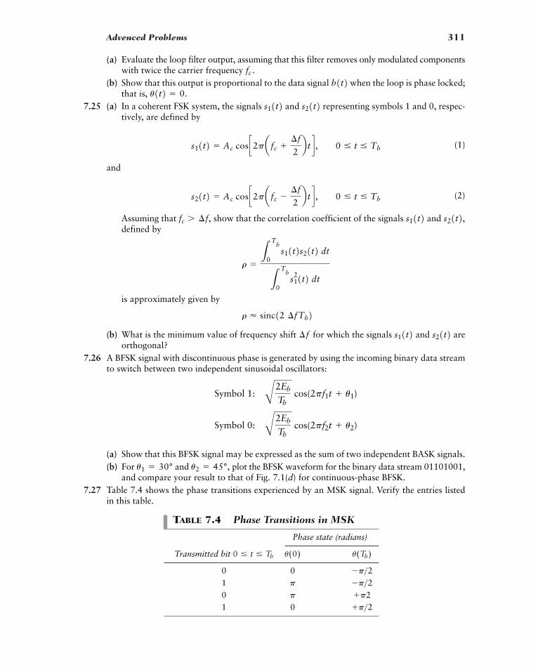
Advenced Problems 311
(a) Evaluate the loop filter output, assuming that this filter removes only modulated componentswith twice the carrier frequency
(b) Show that this output is proportional to the data signal when the loop is phase locked;that is,
7.25 (a) In a coherent FSK system, the signals and representing symbols 1 and 0, respec-tively, are defined by
(1)
and
(2)
Assuming that show that the correlation coefficient of the signals and defined by
is approximately given by
(b) What is the minimum value of frequency shift for which the signals and areorthogonal?
7.26 A BFSK signal with discontinuous phase is generated by using the incoming binary data streamto switch between two independent sinusoidal oscillators:
(a) Show that this BFSK signal may be expressed as the sum of two independent BASK signals.(b) For and plot the BFSK waveform for the binary data stream 01101001,
and compare your result to that of Fig. 7.1(d) for continuous-phase BFSK.7.27 Table 7.4 shows the phase transitions experienced by an MSK signal. Verify the entries listed
in this table.
u2 � 45°,u1 � 30°
Symbol 0: B2Eb
Tb cos(2pf2t u2)
Symbol 1: B2Eb
Tb cos(2pf1t u1)
s21t2s11t2¢f
r � sinc12 ¢fTb2
r �L
Tb
0s11t2s21t2 dt
LT
b
0s121t2 dt
s21t2,s11t2fc � ¢f,
s21t2 � Ac cos c2pa fc �¢f
2b t d , 0 � t � Tb
s11t2 � Ac cos c2pa fc ¢f
2b t d , 0 � t � Tb
s21t2s11t2u1t2 � 0.
b1t2fc .
TABLE 7.4 Phase Transitions in MSK
Phase state (radians)
Transmitted bit
0 0101 0 p>2p2p
�p>2p
�p>2u1Tb2u1020 � t � Tb
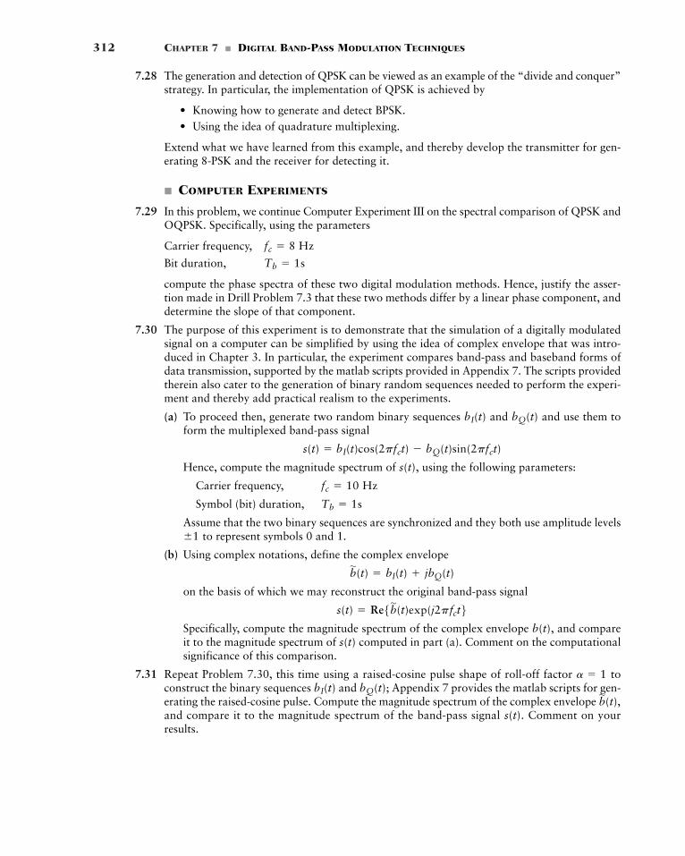
312 CHAPTER 7 � DIGITAL BAND-PASS MODULATION TECHNIQUES
7.28 The generation and detection of QPSK can be viewed as an example of the “divide and conquer”strategy. In particular, the implementation of QPSK is achieved by
• Knowing how to generate and detect BPSK.• Using the idea of quadrature multiplexing.
Extend what we have learned from this example, and thereby develop the transmitter for gen-erating 8-PSK and the receiver for detecting it.
� COMPUTER EXPERIMENTS
7.29 In this problem, we continue Computer Experiment III on the spectral comparison of QPSK andOQPSK. Specifically, using the parameters
Carrier frequency,
Bit duration,
compute the phase spectra of these two digital modulation methods. Hence, justify the asser-tion made in Drill Problem 7.3 that these two methods differ by a linear phase component, anddetermine the slope of that component.
7.30 The purpose of this experiment is to demonstrate that the simulation of a digitally modulatedsignal on a computer can be simplified by using the idea of complex envelope that was intro-duced in Chapter 3. In particular, the experiment compares band-pass and baseband forms ofdata transmission, supported by the matlab scripts provided in Appendix 7. The scripts providedtherein also cater to the generation of binary random sequences needed to perform the experi-ment and thereby add practical realism to the experiments.
(a) To proceed then, generate two random binary sequences and and use them toform the multiplexed band-pass signal
Hence, compute the magnitude spectrum of , using the following parameters:
Carrier frequency,
Symbol (bit) duration,
Assume that the two binary sequences are synchronized and they both use amplitude levelsto represent symbols 0 and 1.
(b) Using complex notations, define the complex envelope
on the basis of which we may reconstruct the original band-pass signal
Specifically, compute the magnitude spectrum of the complex envelope , and compareit to the magnitude spectrum of computed in part (a). Comment on the computationalsignificance of this comparison.
7.31 Repeat Problem 7.30, this time using a raised-cosine pulse shape of roll-off factor toconstruct the binary sequences and ; Appendix 7 provides the matlab scripts for gen-erating the raised-cosine pulse. Compute the magnitude spectrum of the complex envelope and compare it to the magnitude spectrum of the band-pass signal . Comment on yourresults.
s(t)b'(t),
bQ(t)bI(t)a � 1
s(t)b(t)
s(t) � Re5b'(t)exp(j2pfct6b'(t) � bI(t) jbQ(t)
�1
Tb � 1s
fc � 10 Hz
s(t)
s(t) � bI(t)cos(2pfct) � bQ(t)sin(2pfct)
bQ(t)bI(t)
Tb � 1s
fc � 8 Hz
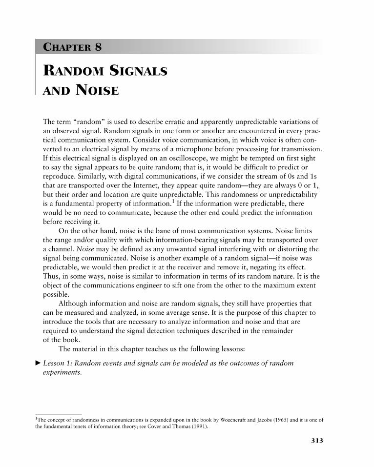
313
1The concept of randomness in communications is expanded upon in the book by Wozencraft and Jacobs (1965) and it is one ofthe fundamental tenets of information theory; see Cover and Thomas (1991).
CHAPTER 8
RANDOM SIGNALS
AND NOISE
The term “random” is used to describe erratic and apparently unpredictable variations ofan observed signal. Random signals in one form or another are encountered in every prac-tical communication system. Consider voice communication, in which voice is often con-verted to an electrical signal by means of a microphone before processing for transmission.If this electrical signal is displayed on an oscilloscope, we might be tempted on first sightto say the signal appears to be quite random; that is, it would be difficult to predict orreproduce. Similarly, with digital communications, if we consider the stream of 0s and 1sthat are transported over the Internet, they appear quite random—they are always 0 or 1,but their order and location are quite unpredictable. This randomness or unpredictabilityis a fundamental property of information.1 If the information were predictable, therewould be no need to communicate, because the other end could predict the informationbefore receiving it.
On the other hand, noise is the bane of most communication systems. Noise limitsthe range and/or quality with which information-bearing signals may be transported overa channel. Noise may be defined as any unwanted signal interfering with or distorting thesignal being communicated. Noise is another example of a random signal—if noise waspredictable, we would then predict it at the receiver and remove it, negating its effect.Thus, in some ways, noise is similar to information in terms of its random nature. It is theobject of the communications engineer to sift one from the other to the maximum extentpossible.
Although information and noise are random signals, they still have properties thatcan be measured and analyzed, in some average sense. It is the purpose of this chapter tointroduce the tools that are necessary to analyze information and noise and that arerequired to understand the signal detection techniques described in the remainder of the book.
The material in this chapter teaches us the following lessons:
� Lesson 1: Random events and signals can be modeled as the outcomes of randomexperiments.
314 CHAPTER 8 � RANDOM SIGNALS AND NOISE
� Lesson 2: Random variables provide a general representation for analyzing, comparing,and processing outcomes of random experiments. Statistical properties of random eventscan be obtained from the expectation of the various functions of these random variables;the expectation should be viewed as an operator.
� Lesson 3: Gaussian random variables play a key role in the analysis of random signalsbecause of the central limit theorem and their mathematical tractability.
� Lesson 4: A random process may be viewed as a family of random variables, indexed by atime parameter. Then we can extend the analysis techniques for random variables to studythe time-variation of random processes.
� Lesson 5: White noise is one of the most important random processes in the study of com-munication systems, both from a practical viewpoint and for the mathematical tractabilityof its statistical properties.
� Lesson 6: Narrowband noise can be analyzed in terms of its in-phase and quadrature com-ponents, in a manner similar to narrowband communication signals.
8.1 Probability and Random Variables
Probability theory is rooted in situations that involve performing an experiment with anoutcome that is subject to chance. That is, if the experiment is repeated, the outcome maydiffer due to the influence of an underlying random phenomenon. Such an experiment isreferred to as a random experiment. For example, the experiment may be the observationof the result of the tossing of a fair coin. In this experiment, the possible outcomes of a trialare “heads” and “tails.”
We ask that a random experiment have the following properties:
1. On any trial of the experiment, the outcome is unpredictable.2. For a large number of trials of the experiment, the outcomes exhibit statistical regu-
larity. That is, a definite average pattern of outcomes is observed if the experiment isrepeated a large number of times.
� RELATIVE-FREQUENCY APPROACH
To elaborate on the concept of statistical regularity, let event A denote one of the possibleoutcomes of a random experiment. For example, in the coin-tossing experiment, event Amay represent “heads.” Suppose that in n trials of the experiment, event A occurs times.We may then assign the ratio to the event A. This ratio is called the relative frequencyof the event A. Clearly, the relative frequency is a nonnegative real number less than or equalto one. That is to say,
(8.1)0 �nA
n� 1
nA>n nA
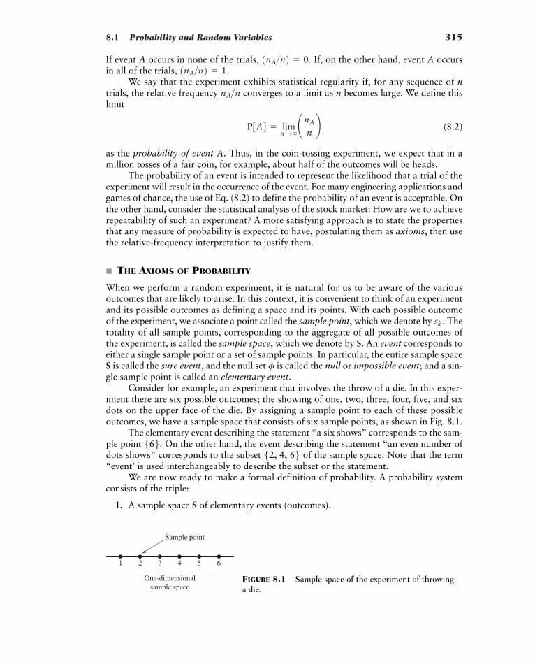
8.1 Probability and Random Variables 315
1 2 3 4 5 6
Sample point
One-dimensionalsample space
FIGURE 8.1 Sample space of the experiment of throwinga die.
If event A occurs in none of the trials, If, on the other hand, event A occursin all of the trials,
We say that the experiment exhibits statistical regularity if, for any sequence of ntrials, the relative frequency converges to a limit as n becomes large. We define thislimit
(8.2)
as the probability of event A. Thus, in the coin-tossing experiment, we expect that in amillion tosses of a fair coin, for example, about half of the outcomes will be heads.
The probability of an event is intended to represent the likelihood that a trial of theexperiment will result in the occurrence of the event. For many engineering applications andgames of chance, the use of Eq. (8.2) to define the probability of an event is acceptable. Onthe other hand, consider the statistical analysis of the stock market: How are we to achieverepeatability of such an experiment? A more satisfying approach is to state the propertiesthat any measure of probability is expected to have, postulating them as axioms, then usethe relative-frequency interpretation to justify them.
� THE AXIOMS OF PROBABILITY
When we perform a random experiment, it is natural for us to be aware of the variousoutcomes that are likely to arise. In this context, it is convenient to think of an experimentand its possible outcomes as defining a space and its points. With each possible outcomeof the experiment, we associate a point called the sample point, which we denote by Thetotality of all sample points, corresponding to the aggregate of all possible outcomes ofthe experiment, is called the sample space, which we denote by S. An event corresponds toeither a single sample point or a set of sample points. In particular, the entire sample spaceS is called the sure event, and the null set is called the null or impossible event; and a sin-gle sample point is called an elementary event.
Consider for example, an experiment that involves the throw of a die. In this exper-iment there are six possible outcomes; the showing of one, two, three, four, five, and sixdots on the upper face of the die. By assigning a sample point to each of these possibleoutcomes, we have a sample space that consists of six sample points, as shown in Fig. 8.1.
The elementary event describing the statement “a six shows” corresponds to the sam-ple point On the other hand, the event describing the statement “an even number ofdots shows” corresponds to the subset of the sample space. Note that the term“event’ is used interchangeably to describe the subset or the statement.
We are now ready to make a formal definition of probability. A probability systemconsists of the triple:
1. A sample space S of elementary events (outcomes).
52, 4, 66566.
f
sk .
P3A4 � limnS�¢nA
n≤
nA>n1nA>n2 � 1.
1nA>n2 � 0.
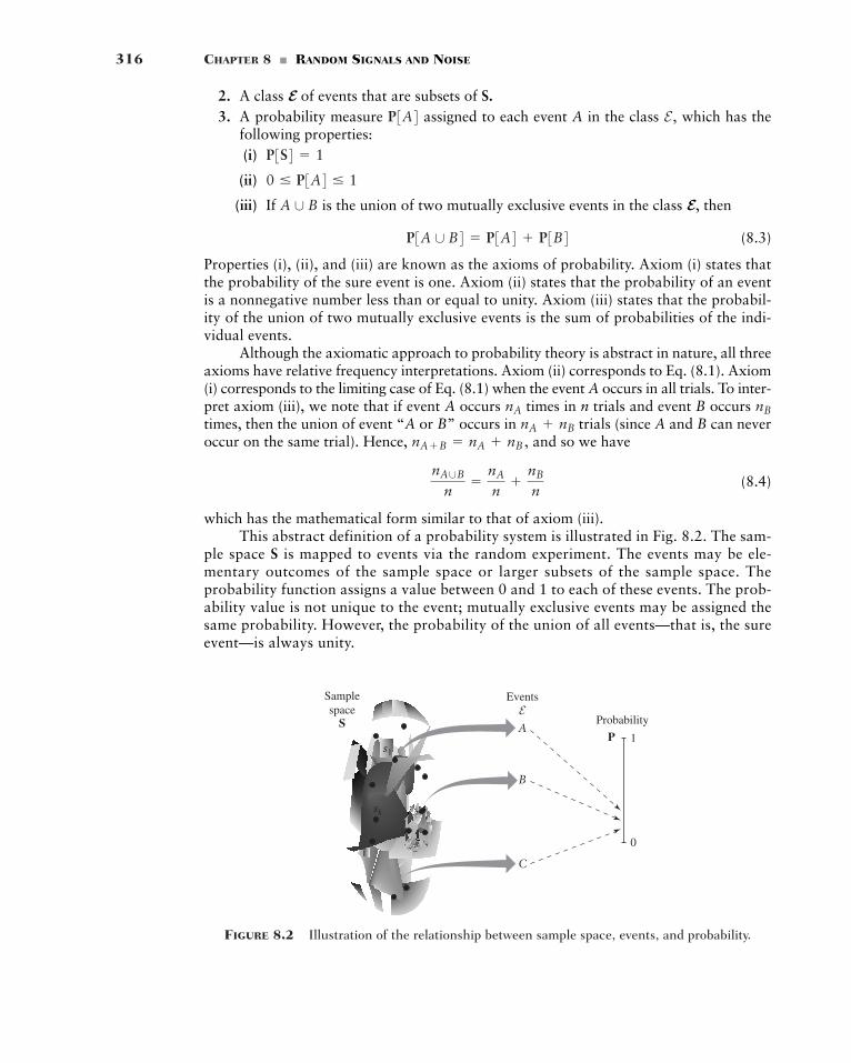
316 CHAPTER 8 � RANDOM SIGNALS AND NOISE
s1
sk
A
E
P
Events
Probability
Samplespace
S1
0
B
C
2. A class E of events that are subsets of S.3. A probability measure assigned to each event A in the class which has the
following properties:(i)
(ii)
(iii) If is the union of two mutually exclusive events in the class E, then
(8.3)
Properties (i), (ii), and (iii) are known as the axioms of probability. Axiom (i) states thatthe probability of the sure event is one. Axiom (ii) states that the probability of an eventis a nonnegative number less than or equal to unity. Axiom (iii) states that the probabil-ity of the union of two mutually exclusive events is the sum of probabilities of the indi-vidual events.
Although the axiomatic approach to probability theory is abstract in nature, all threeaxioms have relative frequency interpretations. Axiom (ii) corresponds to Eq. (8.1). Axiom(i) corresponds to the limiting case of Eq. (8.1) when the event A occurs in all trials. To inter-pret axiom (iii), we note that if event A occurs times in n trials and event B occurstimes, then the union of event “A or B” occurs in trials (since A and B can neveroccur on the same trial). Hence, and so we have
(8.4)
which has the mathematical form similar to that of axiom (iii).This abstract definition of a probability system is illustrated in Fig. 8.2. The sam-
ple space S is mapped to events via the random experiment. The events may be ele-mentary outcomes of the sample space or larger subsets of the sample space. Theprobability function assigns a value between 0 and 1 to each of these events. The prob-ability value is not unique to the event; mutually exclusive events may be assigned thesame probability. However, the probability of the union of all events—that is, the sureevent—is always unity.
nA∪B
n�
nA
n
nB
n
nAB � nA nB ,nA nB
nBnA
P3A ∪ B4 � P3A4 P3B4A ∪ B
0 � P3A4 � 1
P3S4 � 1
E,P3A4
FIGURE 8.2 Illustration of the relationship between sample space, events, and probability.
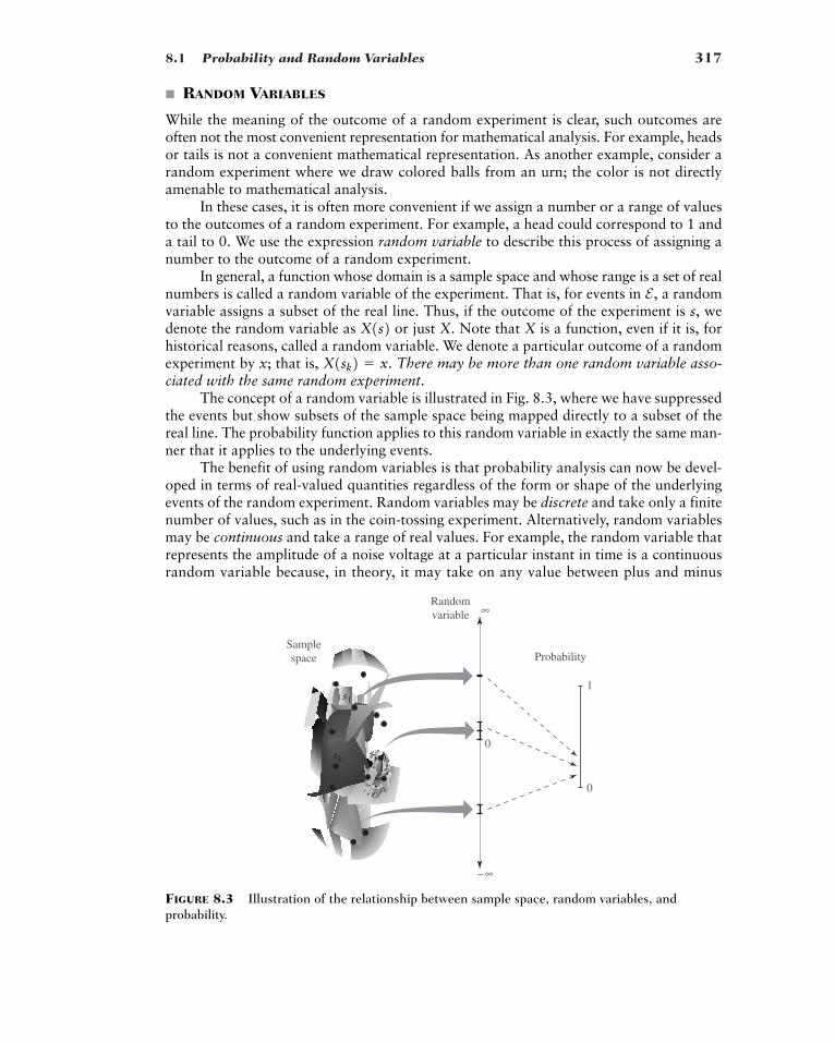
8.1 Probability and Random Variables 317
s1
sk
Samplespace
Randomvariable ∞
–∞
Probability
1
0
0
FIGURE 8.3 Illustration of the relationship between sample space, random variables, andprobability.
� RANDOM VARIABLES
While the meaning of the outcome of a random experiment is clear, such outcomes areoften not the most convenient representation for mathematical analysis. For example, headsor tails is not a convenient mathematical representation. As another example, consider arandom experiment where we draw colored balls from an urn; the color is not directlyamenable to mathematical analysis.
In these cases, it is often more convenient if we assign a number or a range of valuesto the outcomes of a random experiment. For example, a head could correspond to 1 anda tail to 0. We use the expression random variable to describe this process of assigning anumber to the outcome of a random experiment.
In general, a function whose domain is a sample space and whose range is a set of realnumbers is called a random variable of the experiment. That is, for events in a randomvariable assigns a subset of the real line. Thus, if the outcome of the experiment is s, wedenote the random variable as or just X. Note that X is a function, even if it is, forhistorical reasons, called a random variable. We denote a particular outcome of a randomexperiment by x; that is, There may be more than one random variable asso-ciated with the same random experiment.
The concept of a random variable is illustrated in Fig. 8.3, where we have suppressedthe events but show subsets of the sample space being mapped directly to a subset of thereal line. The probability function applies to this random variable in exactly the same man-ner that it applies to the underlying events.
The benefit of using random variables is that probability analysis can now be devel-oped in terms of real-valued quantities regardless of the form or shape of the underlyingevents of the random experiment. Random variables may be discrete and take only a finitenumber of values, such as in the coin-tossing experiment. Alternatively, random variablesmay be continuous and take a range of real values. For example, the random variable thatrepresents the amplitude of a noise voltage at a particular instant in time is a continuousrandom variable because, in theory, it may take on any value between plus and minus
X1sk2 � x.
X1s2E,
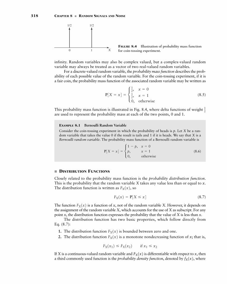
318 CHAPTER 8 � RANDOM SIGNALS AND NOISE
0 1 X
1/2 1/2
FIGURE 8.4 Illustration of probability mass functionfor coin-tossing experiment.
infinity. Random variables may also be complex valued, but a complex-valued randomvariable may always be treated as a vector of two real-valued random variables.
For a discrete-valued random variable, the probability mass function describes the prob-ability of each possible value of the random variable. For the coin-tossing experiment, if it isa fair coin, the probability mass function of the associated random variable may be written as
(8.5)
This probability mass function is illustrated in Fig. 8.4, where delta functions of weight are used to represent the probability mass at each of the two points, 0 and 1.
EXAMPLE 8.1 Bernoulli Random Variable
Consider the coin-tossing experiment in which the probability of heads is p. Let X be a ran-dom variable that takes the value 0 if the result is tails and 1 if it is heads. We say that X is aBernoulli random variable. The probability mass function of a Bernoulli random variable is
(8.6)
� DISTRIBUTION FUNCTIONS
Closely related to the probability mass function is the probability distribution function.This is the probability that the random variable X takes any value less than or equal to x.The distribution function is written as so
(8.7)
The function is a function of x, not of the random variable X. However, it depends onthe assignment of the random variable X, which accounts for the use of X as subscript. For anypoint x, the distribution function expresses the probability that the value of X is less than x.
The distribution function has two basic properties, which follow directly from Eq. (8.7):
1. The distribution function is bounded between zero and one.2. The distribution function is a monotone nondecreasing function of x; that is,
If X is a continuous-valued random variable and is differentiable with respect to x, thena third commonly used function is the probability density function, denoted by wherefX1x2,FX1x2
FX1x12 � FX1x22 if x1 � x2
FX1x2FX1x2
FX1x2FX1x2 � P3X � x4
FX1x2,
P3X � x4 � c 1 � p, x � 0p, x � 10, otherwise
12
P3X � x4 � c 12, x � 012, x � 10, otherwise
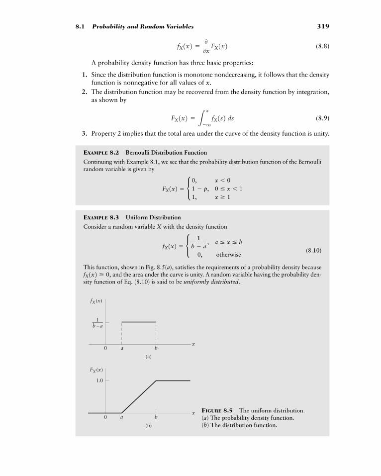
8.1 Probability and Random Variables 319
(8.8)
A probability density function has three basic properties:
1. Since the distribution function is monotone nondecreasing, it follows that the densityfunction is nonnegative for all values of x.
2. The distribution function may be recovered from the density function by integration,as shown by
(8.9)
3. Property 2 implies that the total area under the curve of the density function is unity.
EXAMPLE 8.2 Bernoulli Distribution Function
Continuing with Example 8.1, we see that the probability distribution function of the Bernoullirandom variable is given by
EXAMPLE 8.3 Uniform Distribution
Consider a random variable X with the density function
(8.10)
This function, shown in Fig. 8.5(a), satisfies the requirements of a probability density becauseand the area under the curve is unity. A random variable having the probability den-
sity function of Eq. (8.10) is said to be uniformly distributed.fX1x2 � 0,
fX1x2 � c 1b � a
, a � x � b
0, otherwise
FX1x2 � c 0, x � 01 � p, 0 � x � 11, x � 1
FX1x2 � Lx
�qfX1s2 ds
fX1x2 ��
�xFX1x2
(a)
0
fX (x)
x
b – a
a b
1——
(b)
0
FX (x)
xa b
1.0
FIGURE 8.5 The uniform distribution. (a) The probability density function. (b) The distribution function.
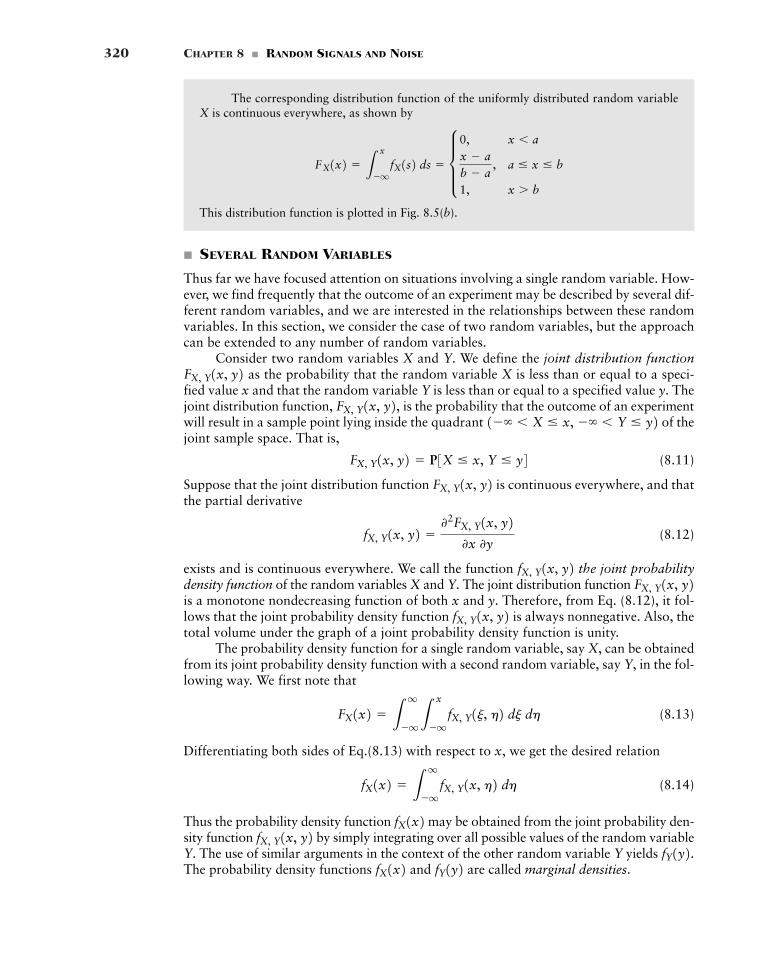
320 CHAPTER 8 � RANDOM SIGNALS AND NOISE
The corresponding distribution function of the uniformly distributed random variableX is continuous everywhere, as shown by
This distribution function is plotted in Fig. 8.5(b).
� SEVERAL RANDOM VARIABLES
Thus far we have focused attention on situations involving a single random variable. How-ever, we find frequently that the outcome of an experiment may be described by several dif-ferent random variables, and we are interested in the relationships between these randomvariables. In this section, we consider the case of two random variables, but the approachcan be extended to any number of random variables.
Consider two random variables X and Y. We define the joint distribution functionas the probability that the random variable X is less than or equal to a speci-
fied value x and that the random variable Y is less than or equal to a specified value y. Thejoint distribution function, is the probability that the outcome of an experimentwill result in a sample point lying inside the quadrant of thejoint sample space. That is,
(8.11)
Suppose that the joint distribution function is continuous everywhere, and thatthe partial derivative
(8.12)
exists and is continuous everywhere. We call the function the joint probabilitydensity function of the random variables X and Y. The joint distribution function is a monotone nondecreasing function of both x and y. Therefore, from Eq. (8.12), it fol-lows that the joint probability density function is always nonnegative. Also, thetotal volume under the graph of a joint probability density function is unity.
The probability density function for a single random variable, say X, can be obtainedfrom its joint probability density function with a second random variable, say Y, in the fol-lowing way. We first note that
(8.13)
Differentiating both sides of Eq.(8.13) with respect to x, we get the desired relation
(8.14)
Thus the probability density function may be obtained from the joint probability den-sity function by simply integrating over all possible values of the random variableY. The use of similar arguments in the context of the other random variable Y yieldsThe probability density functions and are called marginal densities.fY1y2fX1x2 fY1y2.fX, Y1x, y2 fX1x2
fX1x2 � Lq
�qfX, Y1x, h2 dh
FX1x2 � Lq
�qLx
�qfX, Y1j, h2 dj dh
fX, Y1x, y2FX, Y1x, y2fX, Y1x, y2
fX, Y1x, y2 ��2FX, Y1x, y2
�x �y
FX, Y1x, y2FX, Y1x, y2 � P3X � x, Y � y4
1�� � X � x, �� � Y � y2FX, Y1x, y2,FX, Y1x, y2
FX1x2 � Lx
�qfX1s2 ds � d 0, x � a
x � ab � a
, a � x � b
1, x � b
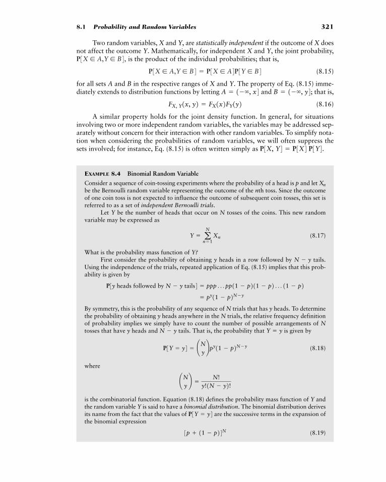
8.1 Probability and Random Variables 321
Two random variables, X and Y, are statistically independent if the outcome of X doesnot affect the outcome Y. Mathematically, for independent X and Y, the joint probability,
is the product of the individual probabilities; that is,
(8.15)
for all sets A and B in the respective ranges of X and Y. The property of Eq. (8.15) imme-diately extends to distribution functions by letting and that is,
(8.16)
A similar property holds for the joint density function. In general, for situationsinvolving two or more independent random variables, the variables may be addressed sep-arately without concern for their interaction with other random variables. To simplify nota-tion when considering the probabilities of random variables, we will often suppress thesets involved; for instance, Eq. (8.15) is often written simply as
EXAMPLE 8.4 Binomial Random Variable
Consider a sequence of coin-tossing experiments where the probability of a head is p and letbe the Bernoulli random variable representing the outcome of the nth toss. Since the outcomeof one coin toss is not expected to influence the outcome of subsequent coin tosses, this set isreferred to as a set of independent Bernoulli trials.
Let Y be the number of heads that occur on N tosses of the coins. This new randomvariable may be expressed as
(8.17)
What is the probability mass function of Y?First consider the probability of obtaining y heads in a row followed by tails.
Using the independence of the trials, repeated application of Eq. (8.15) implies that this prob-ability is given by
By symmetry, this is the probability of any sequence of N trials that has y heads. To determinethe probability of obtaining y heads anywhere in the N trials, the relative frequency definitionof probability implies we simply have to count the number of possible arrangements of Ntosses that have y heads and tails. That is, the probability that is given by
(8.18)
where
is the combinatorial function. Equation (8.18) defines the probability mass function of Y andthe random variable Y is said to have a binomial distribution. The binomial distribution derivesits name from the fact that the values of are the successive terms in the expansion ofthe binomial expression
(8.19)3p 11 � p24NP3Y � y4
¢Ny≤ �
N!y!1N � y2!
P3Y � y4 � ¢Ny≤py11 � p2N�y
Y � yN � y
� py11 � p2N�y
P3y heads followed by N � y tails4 � ppp Á pp11 � p211 � p2Á 11 � p2
N � y
Y � aN
n�1Xn
Xn
P3X, Y4 � P3X4 P3Y4.
FX, Y1x, y2 � FX1x2FY1y2B � 1��, y4;A � 1��, x4
P3X � A,Y � B4 � P3X � A4P3Y � B4P3X � A,Y � B4,
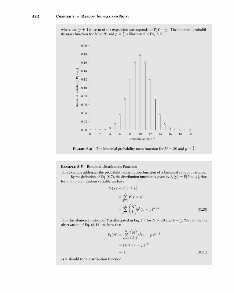
322 CHAPTER 8 � RANDOM SIGNALS AND NOISE
where the term of the expansion corresponds to The binomial probabil-ity mass function for and is illustrated in Fig. 8.6.p � 1
2N � 20P3Y � y4.1y 12st
0 2 4 6 8 10 12 14 16 18 200.00
0.02
0.04
0.06
0.08
0.10
0.12
0.14
0.16
0.18
0.20
Bin
omia
l pro
babi
lity
P[Y
= y]
Random variable Y
FIGURE 8.6 The binomial probability mass function for and p � 12 .N � 20
EXAMPLE 8.5 Binomial Distribution Function
This example addresses the probability distribution function of a binomial random variable.By the definition of Eq. (8.7), the distribution function is given by thus
for a binomial random variable we have
(8.20)
This distribution function of Y is illustrated in Fig. 8.7 for and We can use theobservation of Eq. (8.19) to show that
(8.21)
as it should for a distribution function.
� 1
� 3p 11 � p24NFY1N2 � a
N
k�0¢N
k≤pk11 � p2N�k
p � 12 .N � 20
� ay
k�0¢N
k≤pk11 � p2N�k
� ay
k�0P3Y � k4
FY1y2 � P3Y � y4FY1y2 � P3Y � y4,
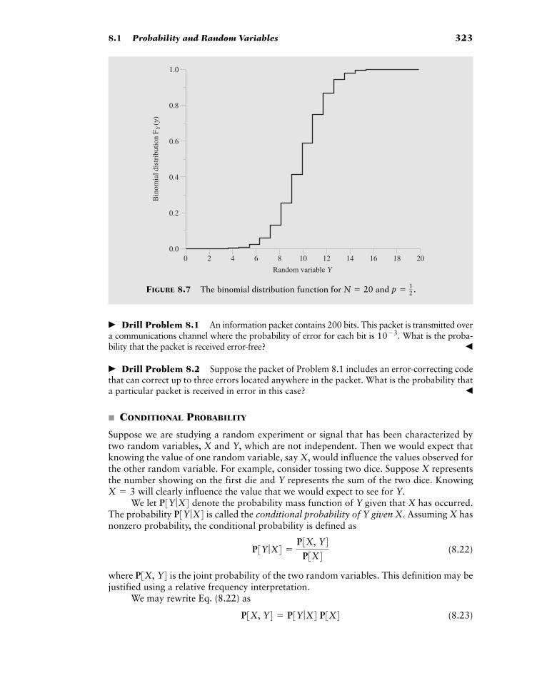
8.1 Probability and Random Variables 323
20 4 6 8 10 12 14 16 18 200.0
0.2
0.4
0.6
0.8
1.0
Bin
omia
l dis
trib
utio
n F Y
(y)
Random variable Y
FIGURE 8.7 The binomial distribution function for and p � 12 .N � 20
� Drill Problem 8.1 An information packet contains 200 bits. This packet is transmitted overa communications channel where the probability of error for each bit is What is the proba-bility that the packet is received error-free? �
� Drill Problem 8.2 Suppose the packet of Problem 8.1 includes an error-correcting codethat can correct up to three errors located anywhere in the packet. What is the probability thata particular packet is received in error in this case? �
� CONDITIONAL PROBABILITY
Suppose we are studying a random experiment or signal that has been characterized bytwo random variables, X and Y, which are not independent. Then we would expect thatknowing the value of one random variable, say X, would influence the values observed forthe other random variable. For example, consider tossing two dice. Suppose X representsthe number showing on the first die and Y represents the sum of the two dice. Knowing
will clearly influence the value that we would expect to see for Y.We let denote the probability mass function of Y given that X has occurred.
The probability is called the conditional probability of Y given X. Assuming X hasnonzero probability, the conditional probability is defined as
(8.22)
where is the joint probability of the two random variables. This definition may bejustified using a relative frequency interpretation.
We may rewrite Eq. (8.22) as
(8.23)P3X, Y4 � P3Y ƒX4 P3X4
P3X, Y4P3Y ƒX4 �
P3X, Y4P3X4
P3Y ƒX4P3Y ƒX4X � 3
10�3.
324 CHAPTER 8 � RANDOM SIGNALS AND NOISE
If we consider the conditional probability of X given Y, we may also write
(8.24)
Equations (8.23) and (8.24) state that the joint probability of two events may be expressedas the product of the conditional probability of one event given the other, and the elemen-tary probability of the other. Note that the conditional probabilities and have the same properties as the various probabilities previously defined.
Situations may exist where the conditional probability and the probabilitiesand are easily determined directly, but the conditional probability is
desired. From Eqs. (8.23) and (8.24), it follows that, provided we may deter-mine by using the relation
(8.25)
This relation is a special form of Bayes’ rule.Suppose that the conditional probability is simply equal to the probability of
occurrence of Y; that is,
(8.26)
Under this condition, the joint probability of X and Y is equal to the product of the indi-vidual probabilities:
(8.27)
It then follows from Eq. (8.24) that In this case, knowledge of the outcomeof a random variable tells us no more about probability of the outcome of the other ran-dom variable than we knew without that knowledge. Random variables X and Y that sat-isfy this condition are said to be statistically independent.
EXAMPLE 8.6 Binary Symmetric Channel
Consider a discrete memoryless channel used to transmit binary data. The channel is said to be dis-crete in that it is designed to handle discrete messages. It is memoryless in the sense that the chan-nel output at any time depends only on the channel input at that time. Due to the unavoidablepresence of noise on the channel, errors are made in the received binary data stream. Specifically,when symbol 1 is sent, occasionally an error is made and symbol 0 is received, and vice versa. Thechannel is assumed to be symmetric, which means that the probability of receiving symbol 1 when0 is sent is the same as the probability of receiving symbol 0 when symbol 1 is sent.
To describe the probabilistic nature of this channel fully, we need two sets of probabilities:
1. The a priori probability of sending binary symbols 0 and 1 is given by
where X is the random variable representing the transmitted symbol. Note thatso X is a Bernoulli random variable.
2. The conditional probability of error is given by
where Y is the random variable representing the received symbol. The conditional prob-ability is the probability that symbol 0 is received given that symbol 1was sent.
P3Y � 0 ƒX � 14P3Y � 1 ƒX � 04 � P3Y � 0 ƒX � 14 � p
p0 p1 � 1,
P3X � x4 � bp0 x � 0p1 x � 1
P3X ƒY4 � P3X4.P3X, Y4 � P3X4 P3Y4
P3Y ƒX4 � P3Y4P3Y ƒX4
P3Y ƒX4 �P3X ƒY4 P3Y4
P3X4P3Y ƒX4 P3X4 0,
P3Y ƒX4P3Y4P3X4 P3X ƒY4P3X ƒY4P3Y ƒX4
P3X, Y4 � P3X ƒY4 P3Y4
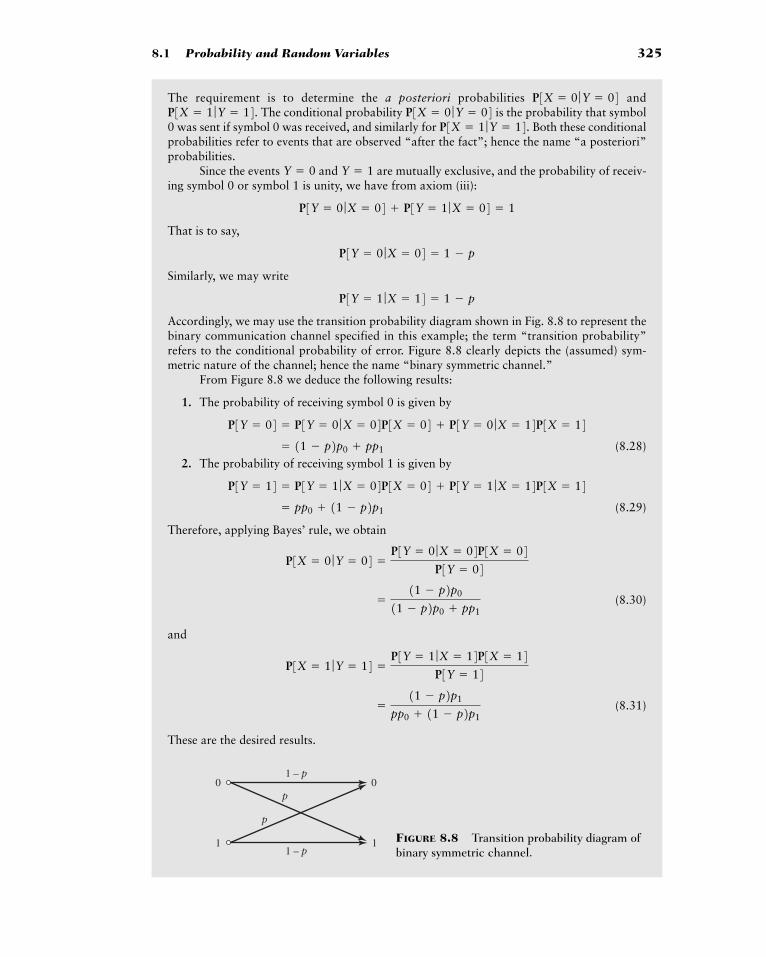
8.1 Probability and Random Variables 325
0 0p
p
1 – p
1 – p
1 1 FIGURE 8.8 Transition probability diagram ofbinary symmetric channel.
The requirement is to determine the a posteriori probabilities andThe conditional probability is the probability that symbol
0 was sent if symbol 0 was received, and similarly for Both these conditionalprobabilities refer to events that are observed “after the fact”; hence the name “a posteriori”probabilities.
Since the events and are mutually exclusive, and the probability of receiv-ing symbol 0 or symbol 1 is unity, we have from axiom (iii):
That is to say,
Similarly, we may write
Accordingly, we may use the transition probability diagram shown in Fig. 8.8 to represent thebinary communication channel specified in this example; the term “transition probability”refers to the conditional probability of error. Figure 8.8 clearly depicts the (assumed) sym-metric nature of the channel; hence the name “binary symmetric channel.”
From Figure 8.8 we deduce the following results:
1. The probability of receiving symbol 0 is given by
(8.28)2. The probability of receiving symbol 1 is given by
(8.29)
Therefore, applying Bayes’ rule, we obtain
(8.30)
and
(8.31)
These are the desired results.
�11 � p2p1
pp0 11 � p2p1
P3X � 1 ƒY � 14 �P3Y � 1 ƒX � 14P3X � 14
P3Y � 14
�11 � p2p011 � p2p0 pp1
P3X � 0 ƒY � 04 �P3Y � 0 ƒX � 04P3X � 04
P3Y � 04
� pp0 11 � p2p1
P3Y � 14 � P3Y � 1 ƒX � 04P3X � 04 P3Y � 1 ƒX � 14P3X � 14� 11 � p2p0 pp1
P3Y � 04 � P3Y � 0 ƒX � 04P3X � 04 P3Y � 0 ƒX � 14P3X � 14
P3Y � 1 ƒX � 14 � 1 � p
P3Y � 0 ƒX � 04 � 1 � p
P3Y � 0 ƒX � 04 P3Y � 1 ƒX � 04 � 1
Y � 1Y � 0
P3X � 1 ƒY � 14.P3X � 0 ƒY � 04P3X � 1 ƒY � 14. P3X � 0 ƒY � 04
326 CHAPTER 8 � RANDOM SIGNALS AND NOISE
� Drill Problem 8.3 Continuing with Example 8.6, find the following conditional prob-abilities: and �
� Drill Problem 8.4 Consider a binary symmetric channel for which the conditional prob-ability of error and symbols 0 and 1 occur with equal probability. Calculate the fol-lowing probabilities:
(a) The probability of receiving symbol 0.(b) The probability of receiving symbol 1.(c) The probability that symbol 0 was sent given that symbol 0 is received.(d) The probability that symbol 1 was sent given that symbol 0 is received. �
8.2 Expectation
The probability distribution function, while it provides a complete description of the randomvariable, may include more detail than is necessary in some instances. We may wish to usesimple statistical averages, such as the mean and variance, to describe the random variable.
� MEAN
These statistical averages or expectations are denoted by, for example, for theexpected value of a function of the random variable X. For the case of the expectedvalue of X, we denote the mean using the shorthand For a discrete random variableX, the mean, is the weighted sum of the possible outcomes
(8.32)
where the sum is over all possible outcomes of the random variable X. For a continuous ran-dom variable with a density function the analogous definition of the expected value is
(8.33)
Often the mean value of a random variable is estimated from N observations of the ran-dom variable using the estimator
(8.34)
That is, we estimate the mean of the distribution by averaging over a number of observa-tions of the random variable. This estimator is based on the relative frequency definitionof probability. For example, if the possible outcomes of a random variable Z are
then the estimator becomes
where is the number of times that the observation occurs. We may rewrite thisequation as
Z � ini
mN Z �1 # n1 2 # n2 Á M # nM
N
1, 2, 3, Á , M,
mN X �1N a
N
n�1xn
5x1, x2, Á , xN6,
E3X4 � Lq
�qxfX1x2 dx
fX1x2,� a
Xx P3X � x4
mX � E3X4mX ,
mX .g1.2 E3g1X24
p � 10�4,
P3X � 1 ƒY � 04.P3X � 0 ƒY � 14
8.2 Expectation 327
That is, we expect the more probable outcomes to occur more frequently when a numberof observations are made.
Returning to the general case, if we consider X as a random variable representingobservations of the voltage of a random signal, then the mean value of X represents the aver-age voltage or dc offset of the signal.
� VARIANCE
The variance of a random variable is an estimate of the spread of the probability distribu-tion about the mean. For discrete random variables, the variance, is given by the expec-tation of the squared distance of each outcome from the mean value of the distribution.
(8.35)
For a continuous random variable with density function the analogous definition ofvariance is given by
(8.36)
As is the case for the mean, we may estimate the variance of a random variable from N inde-pendent observations using the formula
(8.37)
We may justify this estimator using the relative frequency interpretation of probability. Forexample, if we use the random variable Z defined previously, we have
(8.38)
The factor appearing on the right-hand side of Eq. (8.38) is due to the assump-tion that the same N observations are used to estimate the mean With this factor, theexpected value of the right-hand side is and, consequently, Eq. (8.37) is an unbiased esti-mator of the variance. We say is an unbiased estimator of g if E3gN4 � E3g4.gN
sZ2
mN .N>1N � 12
�N
N � 1 aM
i�11i � mN Z22 P3Z � i4
�N
N � 1 aM
ni�11i � mN Z22 ni
N
sN Z2
�11 � mN Z22 # n1 12 � mN Z22 # n2 Á 1M � mN Z22 # nM
N � 1
sN X2
�1
N � 1 aN
n�11xn � mN X22
sX2
� Lq
�q1x � mX22fX1x2 dx
fX1x2,� a
X1x � mX22P3X � x4
� E31X � mX224sX
2� Var1X2
sX2 ,
� aM
i�1iP3Z � i4
mN Z � aM
i�1ini
N
328 CHAPTER 8 � RANDOM SIGNALS AND NOISE
If we consider X as a random variable representing observations of the voltage of a ran-dom signal, then the variance represents the ac power of the signal. The second moment of X,
is also called the mean-square value of the random signal and it physically representsthe total power of the signal.
EXAMPLE 8.7 Mean and Variance of a Bernoulli Random Variable
If X is a Bernoulli random variable with parameter p, then the expected value of X is
With the variance of X is given by
� COVARIANCE
Also of importance in the analysis of communication systems are the statistical averagesbetween two random variables. The covariance of two random variables, X and Y, is givenby the expected value of the product of the two random variables,
(8.39)
We may expand this equation to obtain2 (see Problem 8.23)
(8.40)
If the two random variables are continuous with joint density, then the expec-tation term of Eq. (8.40) is given by
(8.41)
If the two random variables happen to be independent, then
(8.42)
as we might intuitively expect. Substituting this result into Eq. (8.40), we find that thecovariance of independent random variables is zero. It should be noted however that
� E3X4E3Y4� L
q
�qxfX1x2 dx L
q
�qyfX1y2 dy
E3XY4 � Lq
�qLq
�qxyfX1x2fY1y2 dx dy
E3XY4 � Lq
�qLq
�qxyfX, Y1x, y2 dx dy
fX, Y1x, y2,Cov1X, Y2 � E3XY4 � mXmY
Cov1X, Y2 � E31X � mX21Y � mY24
� p11 � p2� 1p2 � p32 1p � 2p2 p32� 10 � p2211 � p2 11 � p22p
sX2
� a1
k�01k � mX22P3X � k4
mX � E3X4,� p
� 0 # 11 � p2 1 # pE3X4 � a
1
k�0kP3X � k4
E3X24,
2If the random variables are complex valued, then this expression is modified to where the asterisk denotes complex conjugation. In such a situation, Cov(X, Y) and Cov (Y, X) are unequal.
Cov1X, Y2 � E3XY*4 � mXmY… ,
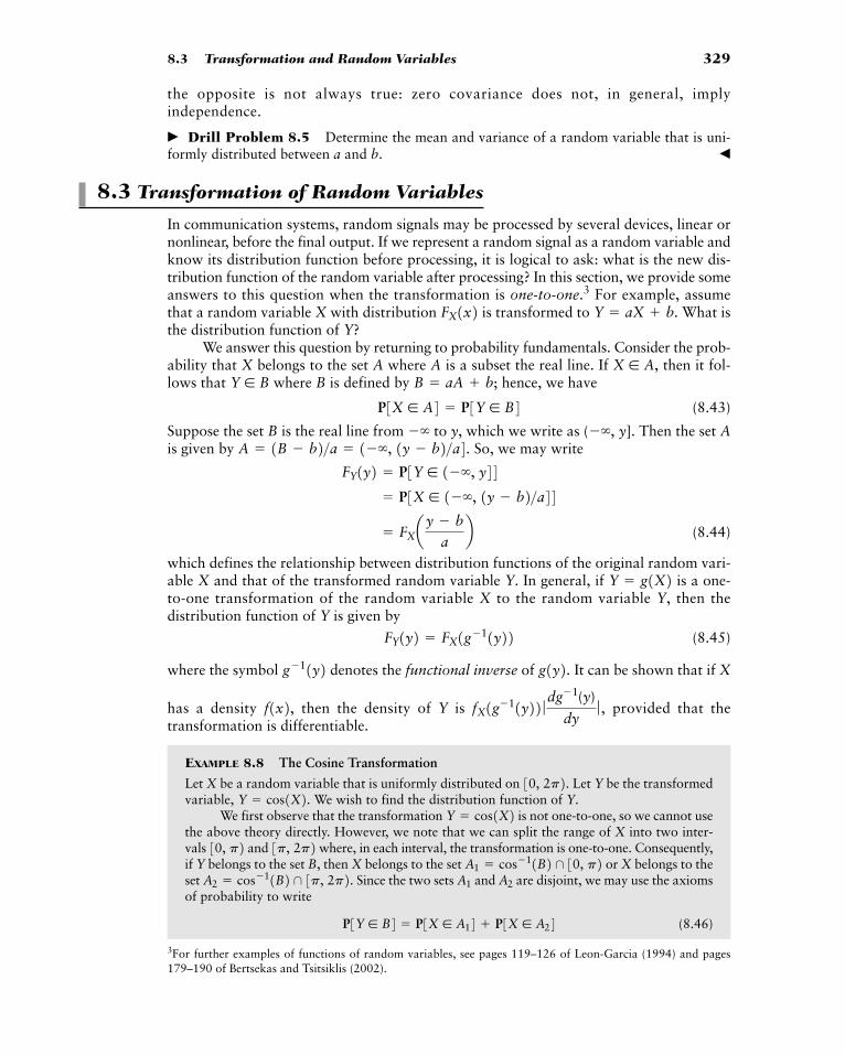
8.3 Transformation and Random Variables 329
the opposite is not always true: zero covariance does not, in general, implyindependence.
� Drill Problem 8.5 Determine the mean and variance of a random variable that is uni-formly distributed between a and b. �
8.3 Transformation of Random Variables
In communication systems, random signals may be processed by several devices, linear ornonlinear, before the final output. If we represent a random signal as a random variable andknow its distribution function before processing, it is logical to ask: what is the new dis-tribution function of the random variable after processing? In this section, we provide someanswers to this question when the transformation is one-to-one.3 For example, assumethat a random variable X with distribution is transformed to What isthe distribution function of Y?
We answer this question by returning to probability fundamentals. Consider the prob-ability that X belongs to the set A where A is a subset the real line. If then it fol-lows that where B is defined by hence, we have
(8.43)
Suppose the set B is the real line from to y, which we write as ( ]. Then the set Ais given by So, we may write
(8.44)
which defines the relationship between distribution functions of the original random vari-able X and that of the transformed random variable Y. In general, if is a one-to-one transformation of the random variable X to the random variable Y, then thedistribution function of Y is given by
(8.45)
where the symbol denotes the functional inverse of It can be shown that if X
has a density then the density of Y is provided that the transformation is differentiable.
EXAMPLE 8.8 The Cosine Transformation
Let X be a random variable that is uniformly distributed on Let Y be the transformedvariable, We wish to find the distribution function of Y.
We first observe that the transformation is not one-to-one, so we cannot usethe above theory directly. However, we note that we can split the range of X into two inter-vals and where, in each interval, the transformation is one-to-one. Consequently,if Y belongs to the set B, then X belongs to the set or X belongs to theset Since the two sets and are disjoint, we may use the axiomsof probability to write
(8.46)P3Y � B4 � P3X � A14 P3X � A24A2A1A2 � cos�11B2 ∩ 3p, 2p2. A1 � cos�11B2 ∩ 30, p23p, 2p230, p2
Y � cos1X2Y � cos1X2. 30, 2p2.
fX1g�11y22 ƒ dg�1(y)
dyƒ ,f1x2,
g1y2.g�11y2FY1y2 � FX1g�11y22
Y � g1X2� FXay � b
ab
� P3X � 1��, 1y � b2>a44FY1y2 � P3Y � 1��, y44
A � 1B � b2>a � 1��, 1y � b2>a4. ��, y��
P3X � A4 � P3Y � B4B � aA b;Y � B
X � A,
Y � aX b.FX1x2
3For further examples of functions of random variables, see pages 119–126 of Leon-Garcia (1994) and pages179–190 of Bertsekas and Tsitsiklis (2002).
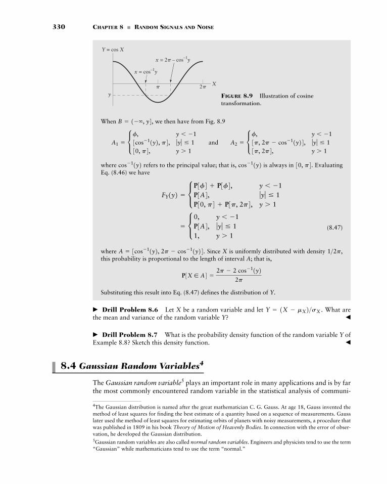
330 CHAPTER 8 � RANDOM SIGNALS AND NOISE
When we then have from Fig. 8.9
where refers to the principal value; that is, is always in EvaluatingEq. (8.46) we have
(8.47)
where Since X is uniformly distributed with density this probability is proportional to the length of interval A; that is,
Substituting this result into Eq. (8.47) defines the distribution of Y.
� Drill Problem 8.6 Let X be a random variable and let What arethe mean and variance of the random variable Y? �
� Drill Problem 8.7 What is the probability density function of the random variable Y ofExample 8.8? Sketch this density function. �
8.4 Gaussian Random Variables4
The Gaussian random variable5 plays an important role in many applications and is by farthe most commonly encountered random variable in the statistical analysis of communi-
Y � 1X � mX2>sX .
P3X � A4 �2p � 2 cos�11y2
2p
1>2p,A � 3cos�11y2, 2p � cos�11y24.
� c 0, y � �1P3A4, ƒy ƒ � 11, y � 1
FY1y2 � c P3f4 P3f4, y � �1P3A4, ƒy ƒ � 1P30, p4 P3p, 2p4, y � 1
30, p4.cos�11y2cos�11y2A1 � c f, y � �13cos�11y2, p4, ƒy ƒ � 130, p4, y � 1
and A2 � c f, y � �13p, 2p � cos�11y24, ƒy ƒ � 13p, 2p4, y � 1
B � 1��, y4,
x = cos–1y
x = 2� – cos–1y
y
Y = cos X
X� 2�
FIGURE 8.9 Illustration of cosinetransformation.
4The Gaussian distribution is named after the great mathematician C. G. Gauss. At age 18, Gauss invented themethod of least squares for finding the best estimate of a quantity based on a sequence of measurements. Gausslater used the method of least squares for estimating orbits of planets with noisy measurements, a procedure thatwas published in 1809 in his book Theory of Motion of Heavenly Bodies. In connection with the error of obser-vation, he developed the Gaussian distribution.5Gaussian random variables are also called normal random variables. Engineers and physicists tend to use the term“Gaussian” while mathematicians tend to use the term “normal.”
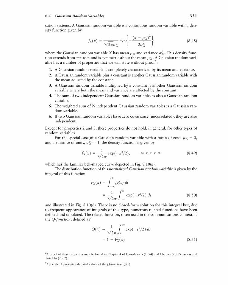
8.4 Gaussian Random Variables 331
cation systems. A Gaussian random variable is a continuous random variable with a den-sity function given by
(8.48)
where the Gaussian random variable X has mean and variance This density func-tion extends from to and is symmetric about the mean A Gaussian random vari-able has a number of properties that we will state without proof6:
1. A Gaussian random variable is completely characterized by its mean and variance.2. A Gaussian random variable plus a constant is another Gaussian random variable with
the mean adjusted by the constant.3. A Gaussian random variable multiplied by a constant is another Gaussian random
variable where both the mean and variance are affected by the constant.4. The sum of two independent Gaussian random variables is also a Gaussian random
variable.5. The weighted sum of N independent Gaussian random variables is a Gaussian ran-
dom variable.6. If two Gaussian random variables have zero covariance (uncorrelated), they are also
independent.
Except for properties 2 and 3, these properties do not hold, in general, for other types ofrandom variables.
For the special case of a Gaussian random variable with a mean of zero, and a variance of unity, the density function is given by
(8.49)
which has the familiar bell-shaped curve depicted in Fig. 8.10(a).The distribution function of this normalized Gaussian random variable is given by the
integral of this function
(8.50)
and illustrated in Fig. 8.10(b). There is no closed-form solution for this integral but, dueto frequent appearance of integrals of this type, numerous related functions have beendefined and tabulated. The related function, often used in the communications context, isthe Q-function, defined as7
(8.51)� 1 � FX1x2Q1x2 �
1
22p Lq
x exp1�s2>22 ds
�1
22p Lx
�q exp1�s2>22 ds
FX1x2 � Lx
�qfX1s2 ds
fX1x2 �1
22p exp1�x2>22, �� � x � �
sX2
� 1,mX � 0,
mX .���sX
2 .mX
fX1x2 �1
22psX
expb�1x � mX22
2sX2 r
6A proof of these properties may be found in Chapter 4 of Leon-Garcia (1994) and Chapter 3 of Bertsekas andTsitsiklis (2002).
7Appendix 4 presents tabulated values of the Q(x).Q-function
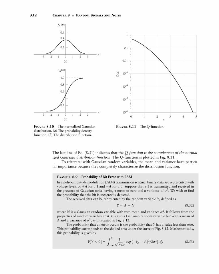
332 CHAPTER 8 � RANDOM SIGNALS AND NOISE
The last line of Eq. (8.51) indicates that the Q-function is the complement of the normal-ized Gaussian distribution function. The Q-function is plotted in Fig. 8.11.
To reiterate: with Gaussian random variables, the mean and variance have particu-lar importance because they completely characterize the distribution function.
EXAMPLE 8.9 Probability of Bit Error with PAM
In a pulse-amplitude modulation (PAM) transmission scheme, binary data are represented withvoltage levels of for a 1 and for a 0. Suppose that a 1 is transmitted and received inthe presence of Gaussian noise having a mean of zero and a variance of We wish to findthe probability that the bit is incorrectly detected.
The received data can be represented by the random variable Y, defined as
(8.52)
where N is a Gaussian random variable with zero mean and variance It follows from theproperties of random variables that Y is also a Gaussian random variable but with a mean ofA and a variance of as illustrated in Fig. 8.12.
The probability that an error occurs is the probability that Y has a value less than zero.This probability corresponds to the shaded area under the curve of Fig. 8.12. Mathematically,this probability is given by
(8.53)P3Y � 04 � L0
�q
1
22ps exp5�1y � A22>2s26 dy
s2,
s2.
Y � A N
s2.�AA
(a)
0
fX (x)
x–1–2–3 321
0.2
0.6
0.4
(b)
0
FX (x)
x–1–2–3 321
0.2
1.0
0.6
0.8
FIGURE 8.10 The normalized Gaussiandistribution. (a) The probability densityfunction. (b) The distribution function.
Q(x
)x
0 1 2 3 4 510–6
10–5
10–4
10–3
0.01
0.1
1
FIGURE 8.11 The Q-function.
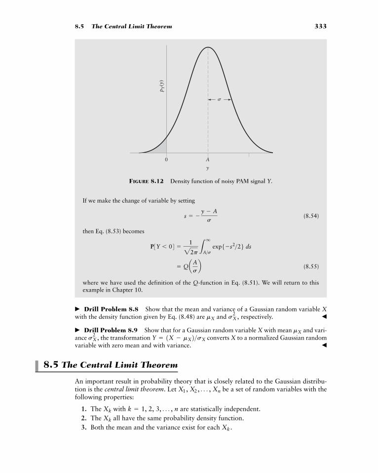
8.5 The Central Limit Theorem 333
If we make the change of variable by setting
(8.54)
then Eq. (8.53) becomes
(8.55)
where we have used the definition of the Q-function in Eq. (8.51). We will return to thisexample in Chapter 10.
� Drill Problem 8.8 Show that the mean and variance of a Gaussian random variable Xwith the density function given by Eq. (8.48) are and respectively. �
� Drill Problem 8.9 Show that for a Gaussian random variable X with mean and vari-ance the transformation converts X to a normalized Gaussian randomvariable with zero mean and with variance. �
8.5 The Central Limit Theorem
An important result in probability theory that is closely related to the Gaussian distribu-tion is the central limit theorem. Let be a set of random variables with thefollowing properties:
1. The with are statistically independent.2. The all have the same probability density function.3. Both the mean and the variance exist for each Xk .
Xk
k � 1, 2, 3, Á , nXk
X1, X2, Á , Xn
Y � 1X � mX2>sXsX2 ,
mX
sX2 ,mX
� QaAsb
P3Y � 04 �1
22p Lq
A>s exp5�s2>26 ds
s � �y � A
s
p Y(y
)0 A
y
FIGURE 8.12 Density function of noisy PAM signal Y.
334 CHAPTER 8 � RANDOM SIGNALS AND NOISE
We do not assume that the density function of the is Gaussian. Let Y be a new ran-dom variable defined as
(8.56)
Then, according to the central limit theorem, the normalized random variable
(8.57)
approaches a Gaussian random variable with zero mean and unit variance as the numberof the random variables increases without limit. That is, as n becomes large,the distribution of Z approaches that of a zero-mean Gaussian random variable with unitvariance, as shown by
(8.58)
This is a mathematical statement of the central limit theorem. In words, the normalized dis-tribution of the sum of independent, identically distributed random variables approachesa Gaussian distribution as the number of random variables increases, regardless of theindividual distributions. Thus, Gaussian random variables are common because they char-acterize the asymptotic properties of many other types of random variables.
When n is finite, the Gaussian approximation of Eq. (8.58) is most accurate in the cen-tral portion of the density function (hence the central limit) and less accurate in the “tails”of the density function.
� COMPUTER EXPERIMENT: SUMS OF RANDOM VARIABLES
In Problem 8.55 toward the end of this chapter, we describe a computer experiment todemonstrate the central limit theorem. In this experiment, we consider the random variable
where the are independent, uniformly distributed random variables on the interval fromto In the computer experiment, we compute 20,000 samples of Z for and
estimate the corresponding density function by forming a histogram of the results. In Fig. 8.13, we compare this histogram (scaled for unit area) to the Gaussian density func-tion having the same mean and variance. As the graph indicates, it does not take manyrandom contributions to approach an overall Gaussian distribution.
The results of this experiment indicate how powerful the central limit theorem is andexplain why Gaussian models are ubiquitous in the analysis of random signals in commu-nications and elsewhere. An added bonus is the mathematical tractability of Gaussian ran-dom variables and the fact that the distribution type is unchanged after linear processing but,of course, the mean and variance of the Gaussian distribution are subjected to change.
� Drill Problem 8.10 Determine the mean and variance of the sum of five independent uni-formly distributed random variables on the interval from to �1.�1
N � 5,1.�1Xi
Z � aN
i�1Xi
FZ1z2S Lz
��
1
22p expb�
s2
2rds
X1, X2, Á , Xn
Z �Y � E3Y4sY
Y � an
k�1Xk
Xk
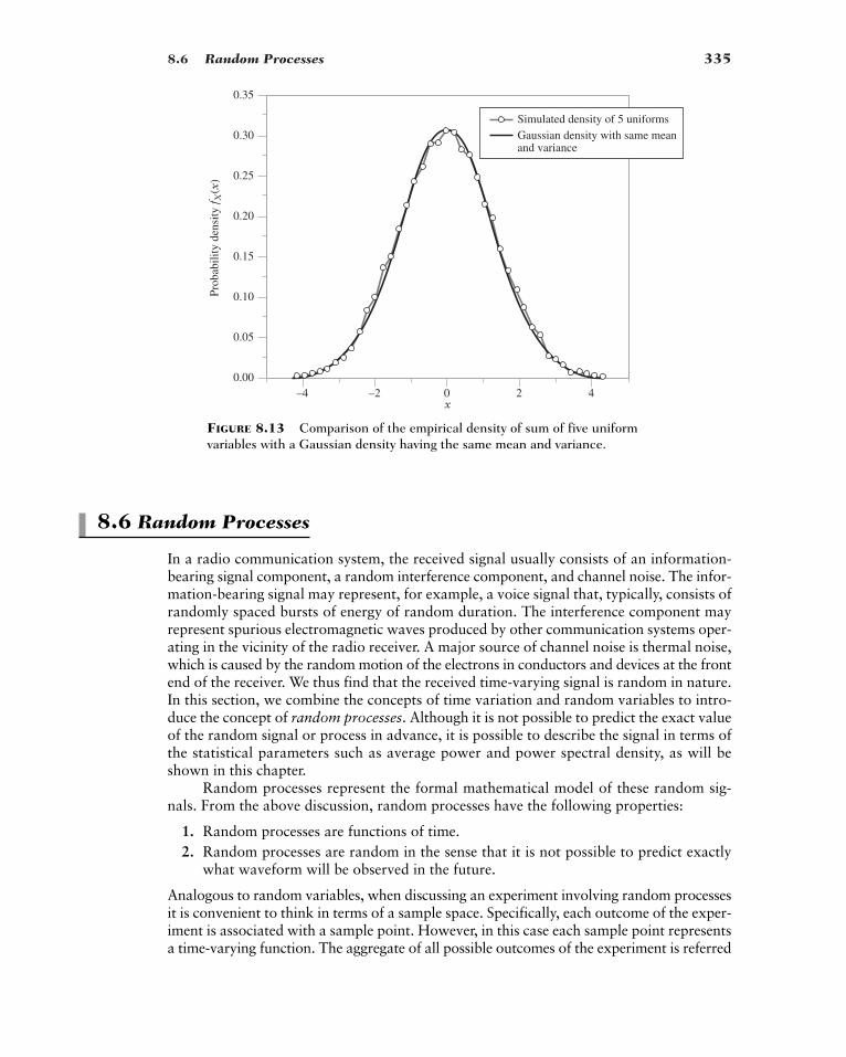
8.6 Random Processes 335
8.6 Random Processes
In a radio communication system, the received signal usually consists of an information-bearing signal component, a random interference component, and channel noise. The infor-mation-bearing signal may represent, for example, a voice signal that, typically, consists ofrandomly spaced bursts of energy of random duration. The interference component mayrepresent spurious electromagnetic waves produced by other communication systems oper-ating in the vicinity of the radio receiver. A major source of channel noise is thermal noise,which is caused by the random motion of the electrons in conductors and devices at the frontend of the receiver. We thus find that the received time-varying signal is random in nature.In this section, we combine the concepts of time variation and random variables to intro-duce the concept of random processes. Although it is not possible to predict the exact valueof the random signal or process in advance, it is possible to describe the signal in terms ofthe statistical parameters such as average power and power spectral density, as will beshown in this chapter.
Random processes represent the formal mathematical model of these random sig-nals. From the above discussion, random processes have the following properties:
1. Random processes are functions of time.2. Random processes are random in the sense that it is not possible to predict exactly
what waveform will be observed in the future.
Analogous to random variables, when discussing an experiment involving random processesit is convenient to think in terms of a sample space. Specifically, each outcome of the exper-iment is associated with a sample point. However, in this case each sample point representsa time-varying function. The aggregate of all possible outcomes of the experiment is referred
Prob
abili
ty d
ensi
ty f X
(x)
x–4 –2 0 2 4
0.00
0.05
0.10
0.15
0.20
0.25
0.30
0.35
Simulated density of 5 uniformsGaussian density with same meanand variance
FIGURE 8.13 Comparison of the empirical density of sum of five uniformvariables with a Gaussian density having the same mean and variance.
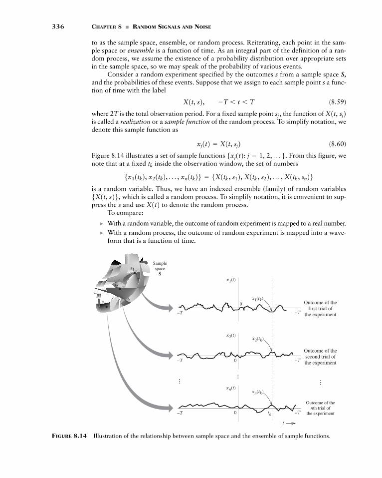
336 CHAPTER 8 � RANDOM SIGNALS AND NOISE
to as the sample space, ensemble, or random process. Reiterating, each point in the sam-ple space or ensemble is a function of time. As an integral part of the definition of a ran-dom process, we assume the existence of a probability distribution over appropriate setsin the sample space, so we may speak of the probability of various events.
Consider a random experiment specified by the outcomes s from a sample space S,and the probabilities of these events. Suppose that we assign to each sample point s a func-tion of time with the label
(8.59)
where 2T is the total observation period. For a fixed sample point the function of is called a realization or a sample function of the random process. To simplify notation, wedenote this sample function as
(8.60)
Figure 8.14 illustrates a set of sample functions From this figure, wenote that at a fixed inside the observation window, the set of numbers
is a random variable. Thus, we have an indexed ensemble (family) of random variableswhich is called a random process. To simplify notation, it is convenient to sup-
press the s and use to denote the random process.To compare:
� With a random variable, the outcome of random experiment is mapped to a real number.� With a random process, the outcome of random experiment is mapped into a wave-
form that is a function of time.
X1t25X1t, s26,5x11tk2, x21tk2, Á , xn1tk26 � 5X1tk , s12, X1tk , s22, Á , X1tk , sn26
tk5xj1t2: j � 1, 2, Á 6.
xj1t2 � X1t, sj2
X1t, sj2sj ,
X1t, s2, �T � t � T
0
Outcome of thefirst trial of
the experiment
Samplespace
S
Outcome of thesecond trial ofthe experiment
Outcome of thenth trial of
the experiment0
...
......
...
xn(tk)
tk +T–T
+T–T
+T–T
x2(tk)
x1(tk)
t
xn(t)
x2(t)
x1(t)
s1
s2
sn 0
FIGURE 8.14 Illustration of the relationship between sample space and the ensemble of sample functions.
8.6 Random Processes 337
At any point in the observation window, the possible outcomes of a random process canbe represented as a random variable. The family of all such random variables, indexed bythe time variable t, forms the random process.
The range of possible random processes is quite large. To restrict this range to ran-dom processes that are both: (i) typical of real-world situations, and (ii) mathematicallytractable, we need two technical conditions, stationarity and ergodicity, which we discussin what follows.
� STATIONARY RANDOM PROCESSES
With real-world random processes, we often find that the statistical characterization of aprocess is independent of the time at which the observations occur. That is, if a randomprocess is divided into a number of time intervals, the various sections of the process exhibitessentially the same statistical properties. Such a process is said to be stationary. Otherwise,it is said to be nonstationary.
This characterization is loosely analogous to linear systems theory, where we definetime-invariant systems as those whose impulse response does not vary with time. This isto be contrasted with time-varying systems, whose impulse response varies with time. Aswith time-invariant systems, stationary random processes are often more mathematicallytractable and simpler to analyze.
To be more precise, let be a random process that is observed at time Letbe the probability distribution function associated with observations of the differ-
ent sample functions of the random process at time Suppose the same random process isobserved at time and the corresponding distribution function is Then if
(8.61)
for all and all we say the process is stationary to the first order. A first-order stationaryrandom process has a distribution function that is independent of time. As a consequence,statistical parameters such as the mean and variance are also independent of time for such aprocess. For example, suppose has the density Then the mean value
(8.62)
does not change with time because the distribution function (and hence the density) are timeinvariant.
Next, consider sampling the random process at two points in time and withthe corresponding joint distribution function Suppose a second set ofobservations are made at times and and the corresponding joint distributionis Then if, for all and we find that
(8.63)
we say the process is stationary to the second order. Stationarity to the second order impliesthat statistical quantities such as covariance and correlation, which we will discuss in thefollowing, do not depend upon absolute time.
The definition of a kth-order stationary random process follows in a similar manner.If the equivalence between distribution functions holds for all time shifts all k, and allpossible observation times then we say the process is strictly stationary. Inother words, a random process is strictly stationary if the joint distribution of any setof random variables obtained by observing the random process is invariant withrespect to the location of the origin t � 0.
X1t2X1t2t1, t2, Á , tk ,t,
FX1t1t2, X1t2t21x1, x22 � FX1t12,X1t221x1, x22t,t1, t2,FX1t1t2, X1t2t21x1, x22. t2 t,t1 t
FX1t12, X1t221x1, x22. t2,t1X1t2
mX � Lq
�qsfX1t121s2 ds � L
q
�qsfX1t1t21s2 ds
fX1t121x2.FX1t121x2t,t1
FX1t1t21x2 � FX1t121x2FX1t1t21x2.t1 t,
t1.FX1t121x2
t1.X1t2
tk ,
338 CHAPTER 8 � RANDOM SIGNALS AND NOISE
� Drill Problem 8.11 A random process is defined by the function
where A and are constants, and is uniformly distributed over the interval 0 to Is Xstationary to the first order? �
� Drill Problem 8.12 Show that a random process that is stationary to the second orderis also stationary to the first order. �
8.7 Correlation of Random Processes
While random processes are, by definition, unpredictable, we often observe that samplesof the process at different times may be correlated. For example, if is large, then wemight also expect to be large, if is small. To quantify this relationship, considerthe covariance of two random variables, defined in Section 8.2, applied to samples of therandom process at times and That is, the covariance of the two random vari-ables and is given by
(8.64)
We define the first term on the right-hand side of Eq. (8.64) as the autocorrelation of therandom process and use the generic notation
(8.65)
where we have used the asterisk to denote conjugation for the case when may be complexvalued. If is stationary to the second order or higher, then Eq. (8.64) may be written as
(8.66)
Stationarity in the second order also implies the mean of the random process is constant.If this mean is zero, then the autocorrelation and covariance functions of a random processare equivalent. The following will show the importance of the autocorrelation function asa descriptor of random processes.
For many applications we do not require a random process to have all of theproperties necessary to be stationary in the second order. In particular, we often onlyrequire:
1. The mean of the random process is a constant independent of time: for all t.
2. The autocorrelation of the random process only depends upon the time difference:for all t and
If a random process has these two properties, then we say it is wide-sense stationary orweakly stationary. Note that wide-sense stationarity does not imply stationarity to the sec-ond order. Neither does stationary to the second order imply wide-sense stationary, as thefirst and second moments may not exist. In the rest of the book, we shall assume that allprocesses of interest are wide-sense stationary.
t.E3X1t2X*1t � t24 � RX1t2,
E3X1t24� mX
� RX1t � s2RX1t, s2 � E3X1t2X*1s24
X1t2 X1t2RX1t, s2 � E3X1t2X*1s24
Cov1X1t12, X1t222 � E3X1t12X1t224 � mX1t12mX1t22X1t22X1t12 t2.t1X1t2
tX1t1 t2 X1t12
2p.uf
X1t, u2 � A cos12pft u2
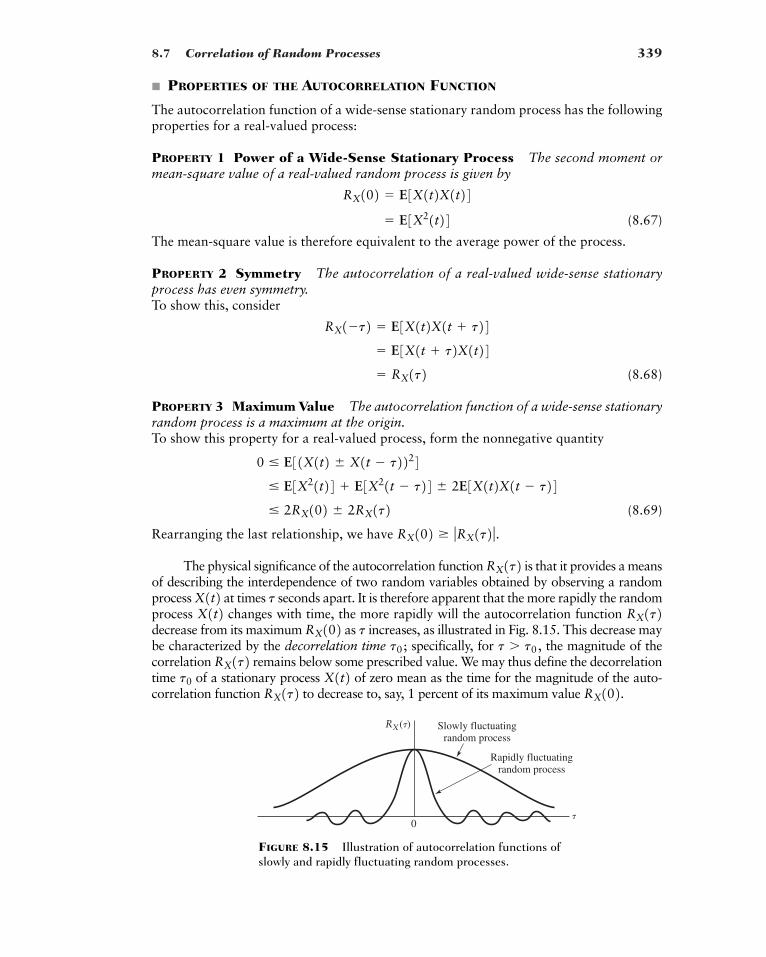
8.7 Correlation of Random Processes 339
� PROPERTIES OF THE AUTOCORRELATION FUNCTION
The autocorrelation function of a wide-sense stationary random process has the followingproperties for a real-valued process:
PROPERTY 1 Power of a Wide-Sense Stationary Process The second moment ormean-square value of a real-valued random process is given by
(8.67)
The mean-square value is therefore equivalent to the average power of the process.
PROPERTY 2 Symmetry The autocorrelation of a real-valued wide-sense stationaryprocess has even symmetry. To show this, consider
(8.68)
PROPERTY 3 Maximum Value The autocorrelation function of a wide-sense stationaryrandom process is a maximum at the origin. To show this property for a real-valued process, form the nonnegative quantity
(8.69)
Rearranging the last relationship, we have
The physical significance of the autocorrelation function is that it provides a meansof describing the interdependence of two random variables obtained by observing a randomprocess at times seconds apart. It is therefore apparent that the more rapidly the randomprocess changes with time, the more rapidly will the autocorrelation function decrease from its maximum as increases, as illustrated in Fig. 8.15. This decrease maybe characterized by the decorrelation time specifically, for the magnitude of thecorrelation remains below some prescribed value. We may thus define the decorrelationtime of a stationary process of zero mean as the time for the magnitude of the auto-correlation function to decrease to, say, 1 percent of its maximum value RX102.RX1t2 X1t2t0
RX1t2 t � t0,t0;tRX102 RX1t2X1t2 tX1t2
RX1t2RX102 � ƒRX1t2 ƒ .
� 2RX102 � 2RX1t2� E3X21t24 E3X21t � t24 � 2E3X1t2X1t � t24
0 � E31X1t2 � X1t � t2224
� RX1t2� E3X1t t2X1t24
RX1�t2 � E3X1t2X1t t24
� E3X21t24RX102 � E3X1t2X1t24
0
Slowly fluctuatingrandom process
Rapidly fluctuatingrandom process
RX(�)
�
FIGURE 8.15 Illustration of autocorrelation functions ofslowly and rapidly fluctuating random processes.
340 CHAPTER 8 � RANDOM SIGNALS AND NOISE
EXAMPLE 8.10 Autocorrelation of a Random Cosine Process
Let be a random process defined by
where the amplitude A and frequency are known, but is uniformly distributed on the inter-val between 0 and This is a special type of random process where a single parameter defines the sample function for all time. The requirement is to find the autocorrelation of
The autocorrelation is given by
Applying the trigonometric identity to this rela-tion, we obtain
Since is uniformly distributed between 0 and we have
Consequently, the expression for the autocorrelation reduces to
The autocorrelation clearly only depends upon the time difference in this example, and theprocess can be shown to be wide-sense stationary.
� Drill Problem 8.13 Let be a random process defined by
where A is uniformly distributed between 0 and 1, and is constant. Determine the autocorre-lation function of X. Is X wide-sense stationary? �
� ERGODICITY
To determine the statistical properties of random processes, we usually have to computeexpectations. The expectation of a random process at a particular point in time requiresseparate independent realizations of the random process. For example, for a random process,
with N equiprobable realizations the expected value andsecond moment of the random process at time are respectively given by the ensem-ble averages
(8.70)
and
(8.71)
If the process is wide-sense stationary, then the mean value and second moment computedby these two equations do not depend upon the time tk .
E3X21tk24 �1N a
N
j�1xj
21tk2
E3X1tk24 �1N a
N
j�1xj1tk2
t � tk5xj1t2: j � 1, 2, Á , N6,X1t2
f
X1t2 � A cos12pft2X1t2
t
RX1t, t � t2 �A2
2cos12pft2
� 0
�1
4psin14pft � 2pft 2u2 `
0
2p
E3cos14pft � 2pft 2u24 �1
2p L2p
0 cos14pft � 2pft 2u2 du
2p,u
RX1t, t � t2 �A2
2cos12pft2
A2
2E3cos14pft � 2pft 2u24
2 cos A cos B � cos1A � B2 cos1A B2� A2E3cos12pft u2 cos12pf1t � t2 u24
RX1t, t � t2 � E3X1t2X1t � t24X1t2.u2p.
uf
X1t2 � A cos12pft u2X1t2
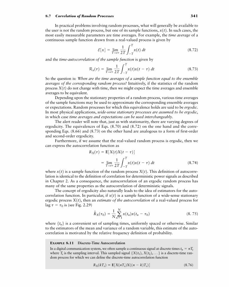
8.7 Correlation of Random Processes 341
In practical problems involving random processes, what will generally be available tothe user is not the random process, but one of its sample functions, In such cases, themost easily measurable parameters are time averages. For example, the time average of acontinuous sample function drawn from a real-valued process is given by
(8.72)
and the time-autocorrelation of the sample function is given by
(8.73)
So the question is: When are the time averages of a sample function equal to the ensembleaverages of the corresponding random process? Intuitively, if the statistics of the randomprocess do not change with time, then we might expect the time averages and ensembleaverages to be equivalent.
Depending upon the stationary properties of a random process, various time averagesof the sample functions may be used to approximate the corresponding ensemble averagesor expectations. Random processes for which this equivalence holds are said to be ergodic.In most physical applications, wide-sense stationary processes are assumed to be ergodic,in which case time averages and expectations can be used interchangeably.
The alert reader will note that, just as with stationarity, there are varying degrees ofergodicity. The equivalences of Eqs. (8.70) and (8.72) on the one hand and the corre-sponding Eqs. (8.66) and (8.73) on the other hand are analogous to a form of first-orderand second-order ergodicity.
Furthermore, if we assume that the real-valued random process is ergodic, then wecan express the autocorrelation function as
(8.74)
where is a sample function of the random process This definition of autocorre-lation is identical to the definition of correlation for deterministic power signals as describedin Chapter 2. As a consequence, the autocorrelation of an ergodic random process hasmany of the same properties as the autocorrelation of deterministic signals.
The concept of ergodicity also naturally leads to the idea of estimators for the auto-correlation function. In particular, if is a sample function of a wide-sense stationaryergodic process then an estimate of the autocorrelation of a real-valued process forlag is (see Fig. 2.29)
(8. 75)
where is a convenient set of sampling times, uniformly spaced or otherwise. Similarto the estimators of the mean and variance of a random variable, this estimate of the auto-correlation is motivated by the relative frequency definition of probability.
EXAMPLE 8.11 Discrete-Time Autocorrelation
In a digital communication system, we often sample a continuous signal at discrete times where is the sampling interval. This sampled signal is a discrete-time ran-dom process for which we can define the discrete-time autocorrelation function
(8.76)RX1kTs2 � E3X1nTs2X11n � k2Ts245X1t12, X1t22, Á 6Ts
tn � nTs
5tn6RN X1t02 �
1N a
N
n�1x1tn2x1tn � t02
t � t0
X1t2, x1t2
X1t2.x1t2� lim
TS�
12T L
T
�Tx1t2x1t � t2 dt
RX1t2 � E3X1t2X1t � t24
X1t2
Rx1t2 � limTS�
12T L
T
�Tx1t2x1t � t2 dt
E3x4 � limTS�
12T L
T
�Tx1t2 dt
x1t2.
342 CHAPTER 8 � RANDOM SIGNALS AND NOISE
where the expectation is the usual ensemble average. As suggested in this section, we may wishto estimate this autocorrelation by performing a time average over a particular sample func-tion. This time average, over N samples of the sample function is defined as
(8.77)
In Fig. 8.16(a), we plot a random signal as a function of time. For this signal, the time-aver-aged autocorrelation of the random signal is shown in Fig. 8.16(b). The horizontal axis rep-resents the time lag in sample periods. Although the signal is quite random in the time domain,it has a smooth autocorrelation function as shown in Fig. 8.16(b).
t
Rx1kTs2 �1N a
N
n�1x1nTs2x11n � k2Ts2
x1t2,
Time (samples)(a)
Am
plitu
de
0 200 400 600 800
0
–1.0
1.0
Time offset (samples)(b)
Aut
ocor
rela
tion
–20 –10 0 10 20–50
0
50
100
150
200
250
FIGURE 8.16 Illustration of (a) a random signal, and (b) itsautocorrelation.
8.8 Spectra of Random Signals 343
� Drill Problem 8.14 A discrete-time random process isdefined by
where is a random process with autocorrelation function , where is the delta function. What is the autocorrelation function Is the process
wide-sense stationary? �
8.8 Spectra of Random Signals
As described above, a random signal may be viewed as belonging to an ensemble of signals,generated by some probabilistic mechanism. Hence, no two signals exhibit the same vari-ation in time. Let denote a sample function of a random process Figure 8.17shows a plot of the waveform of on the interval We may define theFourier transform of the sample function as
(8.78)
This transform converts the sample function to a new sample function 8 Wedefine the collection (ensemble) of all such new sample functions as the new randomprocess Effectively, the Fourier transform has converted a family of randomvariables indexed by parameter t to a new family of random variablesindexed by parameter .
From the discussion of Chapter 2, we recall that the power spectral density of the sam-ple function over the interval is where is the Fouriertransform of This power spectral density will depend on the particular sample func-tion drawn from the ensemble. Accordingly, to obtain the power spectral density ofthe random process, we must perform an ensemble-averaging operation and then take thelimit as T approaches infinity.
The ensemble-averaging operation requires using the probability distribution of theensemble. The value of is held fixed while averaging over the ensemble. For the pre-sent discussion, it is sufficient to acknowledge the ensemble-averaging operation byusing the expectation operator E. We thus write the ensemble-averaged value of the
f
x1t2 xT1t2. jT1f2ƒjT1f2 ƒ2>2T�T � t � Tx1t2f
�T1f2X1t2�T1f2.jT1f2.xT1t2
jT1f2 � Lq
�qxT1t2 exp(�j2pft) dt
xT1t2 �T � t � T.xT1t2 X1t2.x1t2
5Yn6 RY1n, m2 � E3YnYm4? d1n2RZ1n2 � s2d1n25Zn6Yn � a0Zn a1Zn�1
5Yn: n � Á , �1, 0, 1, 2, Á 6
8We previously have used the notation to denote a Fourier-transform pair. However, the use ofto represent the random process introduces a possible ambiguity in notation. Hence, in this section we use
as a Fourier-transform pair of sample functions, and as a Fourier-transform pairof random processes.
X1t2 Δ �1f2x1t2 Δ j1f2X1t2 x1t2 Δ X1f2
xT (t)
–T +T
FIGURE 8.17 Sample function of a random process.
344 CHAPTER 8 � RANDOM SIGNALS AND NOISE
new random process as and the corresponding power spectral den-sity of the random process as
(8.79)
It is important to note that in Eq. (8.79), the ensemble averaging must be performedbefore the limit is taken. Also critical to this definition is that the process be wide-sense stationary.
This approach of determining the power spectral density through an ensemble aver-age may be used to motivate an estimator of the power spectral density given a samplefunction of an ergodic stationary process. In Section 2.10, we saw how the discrete Fouriertransform (DFT) may be used to numerically approximate the Fourier transform. In par-ticular, if are uniformly spaced samples of a function at
then the discrete Fourier transform is defined as
(8.80)
where and are samples of the frequency-domain response atConsequently, we may estimate the power spectral density of a random process
by the following three steps:
1. Partition the sample function into M sections of length and sample atintervals
2. Perform a DFT on each section of length Let whererepresent the M DFT outputs, one set for each section.
3. Average the magnitude squared of each DFT, and then the power spectral densityestimate is given by
(8.81)
This result clearly relies on the process being ergodic.
� PROPERTIES OF THE POWER SPECTRAL DENSITY
The power spectral density and the autocorrelation function of a wide-sensestationary random process form a Fourier-transform pair in the variables and In par-ticular, the same Weiner–Khintchine relations that apply to deterministic processes alsorelate the power spectral density and autocorrelation function of a random process, asshown by
(8.82)
and
(8.83)RX1t2 � Lq
�qSX1f2 exp1j2pft2 df
SX1f2 � Lq
�qRX1t2 exp1�j2pft2 dt
t.fRX1t2SX1f2
�1M a
M�1
m�0` aN�1
n�0xnmNWkn ` 2, k � 0, Á , M � 1
SNX¢ kNTS≤ �
1M a
M�1
m�0ƒjkmN ƒ2
m � 0, Á , M � 15jkmN6NTs .
Ts .NTsx1t2
f � k>NTs .5jk6W � exp1�j2p>N2jk � a
N�1
n�0xnWkn
t � nTs ,x1t25xn: n � 0, 1, Á , N � 16
SX1f2 � limTS�
12T
E3 ƒ�T1f2 ƒ24X1t2 E3 ƒ�T1f2 ƒ24ƒ�T1f2 ƒ2
8.8 Spectra of Random Signals 345
Equations (8.82) and (8.83) are the basic relations of the spectral analysis theory of ran-dom processes. The Weiner–Khintchine relations show that if either the autocorrelationor the power spectral density of the random process is known, the other may be foundexactly.
We can use this pair of relations to derive some general properties of the power spec-tral density of a wide-sense stationary process.
PROPERTY 1 Mean-Square Value The mean-square value of a stationary process equalsthe total area under the graph of the power spectral density; that is,
(8.84)
This property follows directly from Eq. (8.83) by putting and noting that
PROPERTY 2 Nonnegativity The power spectral density of a stationary random processis always nonnegative; that is,
(8.85)
This follows from the definition of the power spectral density given in Eq. (8.79).
PROPERTY 3 Symmetry The power spectral density of a real random process is an evenfunction of frequency; that is,
(8.86)
This property is readily obtained by first substituting for in Eq. (8.82).
Next, substituting for and recognizing that for a real process, weobtain
which is the desired result.
PROPERTY 4 Filtered Random Processes If a stationary random process withspectrum is passed through a linear filter with frequency response the spectrumof the stationary output random process is given by
(8.87)
This result is analogous to that obtained for deterministic signals.9SY1f2 � ƒH1f2 ƒ2SX1f2
Y1t2 H1f2,SX1f2 X1t2
SX1�f2 � Lq
�qRX1t2 exp1�j2pft2 dt � SX1f2
RX1�t2 � RX1t2t,�t
SX1�f2 � Lq
�qRX1t2 exp1j2pft2 dt
f�f
SX1�f2 � SX1f2
SX1f2 � 0, for all f
RX102 � E3 ƒX1t2 ƒ24t � 0
E3 ƒX1t2 ƒ24 � Lq
�qSX1f2 df
9The proof of this result for deterministic signals follows from the convolution theorem of Section 2.2. The prooffor random processes may be found in Chapter 1 of Haykin (2001).
346 CHAPTER 8 � RANDOM SIGNALS AND NOISE
EXAMPLE 8.12 Filtering a Random Sinusoid
A random signal with autocorrelation function
is processed by a causal filter with impulse response that is zero for negative time to pro-duce the new random process
If the filter has an impulse response corresponding to the frequency response
(8.88)
what is the autocorrelation function of From Property 4 of power spectral densities of random processes, we have that the spec-
tral density of is given by
We may use the Fourier-transform pair
(8.89)
to obtain the spectral density Hence,
where the last line anticipates the sifting property of the Dirac delta function. Using the inverseFourier transform of and evaluating of Eq. (8.88) at we get
We thus see that, similar to deterministic sinusoids, linear filtering does not affect the frequencyof a random sinusoid.
� Drill Problem 8.15 For the discrete-time process of Problem 8.14, use the discreteFourier transform to approximate the corresponding spectrum. That is, compute and sketch
If the sampling in the time domain is at where what frequencydoes the integer k correspond to? �
n � 0, 1, 2, Á , N � 1,n>Ts
SY1k2 � aN�1
n�0RY1n2Wkn
RY1t2 �1
1 12pRCfc22 cos12pfct2f � fc ,H1f2SY(f )
�12
ƒH1fc2 ƒ23d1f � fc2 d1f fc24SY1f2 �
12
ƒH1f2 ƒ23d1f � fc2 d1f fc24SX1f2.
cos12pfct2 Δ123d1f � fc2 d1f fc24
SY1f2 � ƒH1f2 ƒ2SX1f2Y1t2
Y1t2?H1f2 �
11 j2pRCf
Y1t2 � Lt
0h1t � s2X1s2 ds
h(t)
RX1t2 �A2
2cos12pfct2
X1t2
8.9 Gaussian Processes 347
8.9 Gaussian Processes
Up to this point in our discussion, we have presented the theory of random processes in gen-eral terms. In the remainder of this chapter, we consider this theory in the context of some impor-tant random processes that are commonly encountered in the study of communication systems.
We have seen how Gaussian random variables play a fundamental role in communi-cation systems because (i) many physical processes that generate noise in communicationsystems can be considered approximately Gaussian distributed; and (ii) the Gaussian ran-dom variable is mathematically tractable and therefore convenient to deal with.
Similarly, a Gaussian process plays an important role in the study of random processesfor two reasons. First, the Gaussian process has many properties that make analytic resultspossible. Second, the random processes produced by physical phenomena are often suchthat a Gaussian model is appropriate.
Before we define a Gaussian process, we must provide some background regardingthe joint distribution of multiple Gaussian random variables. The joint distribution of NGaussian random variables may be written as10
(8.90)
which is called the multi-variate Gaussian distribution. In Eq. (8.90), the respective quan-tities are:
is the N-by-N covariance matrix with individual elements given by
The notation denotes the determinant of matrix With this definition of the multi-variate Gaussian distribution we have a basis for defining a Gaussian random process.
A random process with t taking values in the set T, is said to be a Gaussianprocess if, for any integer k and any subset of T, the k random variables
is jointly Gaussian distributed. That is, for any k,has a density equivalent to Eq. (8.90).
A Gaussian process has the following properties:
1. If a Gaussian process is wide-sense stationary, then it is also stationary in the strict sense.2. If a Gaussian process is applied to a stable linear filter, then the random process
produced at the output of the filter is also Gaussian.3. If integration is defined in the mean-square sense, then we may interchange the order
of the operations of integration and expectation with a Gaussian random process.11
This first property comes from observing that if a Gaussian process is wide-sense stationary, then(i) its mean does not vary with time, and (ii) the elements of the covariance matrix onlydepend on the time difference and not on the absolute t. Since the N-dimensional jointdistribution of samples of a Gaussian process only depends on the mean and covariance throughEq. (8.90), a wide-sense stationary Gaussian process is also strictly stationary.
ti � tj ,¶ij
Y1t2
fX1t12,Á, X1tk21x1, Á , xk25X1t12, X1t22, Á , X1tk26 5t1, t2, Á , tk6X1t2,¶.ƒ ¶ ƒ
¶ij � Cov1Xi , Xj2∂M � 1E3X14, E3X24, Á , E3XN42 is the N-dimensional vector of meansx � 1x1, x2, Á , xN2 is the corresponding vector of indeterminatesX � 1X1, X2, Á , XN2 represents an N-dimensional vector of Gaussian random variables
fX1x2 �1
12p2N>2 ƒ ∂ ƒ1>2 exp5�1x � M2¶�11x � M2T>26
10See Chapter 4 of Leon-Garcia (1994).11See Chapter 6 of Leon-Garcia (1994). The mean-square convergence of to Y implies that
E[(Y � Yn)2] � 0limnS �
5Yn6
348 CHAPTER 8 � RANDOM SIGNALS AND NOISE
The second property comes from observing that the filtering operation can be written as
(8.91)
if we use the following three facts:
1. The integral of Eq. (8.91) is defined as the mean-square limit of the sums
Hence, we observe that the right-hand side is a weighted sum of the Gaussian ran-dom variables
2. Recall from the properties of Gaussian random variables that a weighted sum ofGaussian random variables is another Gaussian random variable.
3. If a sequence of Gaussian random variables converges in the mean-square sense, thenthe result is a Gaussian random variable.
Together these three facts12 can be used to prove that is also a Gaussian randomprocess.
The third property of Gaussian processes implies that if is given by Eq. (8.91)then the mean of the output is given by
These results are very useful in communication systems, where linear filtering of randomprocesses occurs quite often.
� Drill Problem 8.16 Is the discrete-time process defined by and
a Gaussian process, if is Gaussian? Assume that Justify your answer. �
8.10 White Noise
The noise analysis of communication systems is often based on an idealized noise process calledwhite noise. The power spectral density of white noise is independent of frequency. White noiseis analogous to the term “white light” in the sense that all frequency components are present inequal amounts. We denote the power spectral density of a white noise process as
(8.92)
where the factor has been included to indicate that half the power is associated with positivefrequencies and half with negative frequencies, as illustrated in Fig. 8.18(a). The dimensions
12
SW1f2 �N0
2
W1t2
|a | � 1.Wn
Yn1 � aYn Wn
Y0 � 05Yn: n � 0, 1, 2, Á 6
� mY1t2� L
t
0h1t � s2E3X1s24 ds
E3Y1t24 � E cLt
0h1t � s2X1s2 ds d
Y1t2Y1t2
X1i ¢s2.Y1t2 � lim
¢sS0 ai h1t � i ¢s2x1i ¢s2 ¢s
Y1t2 � Lt
0h1t � s2X1s2 ds
12The invariance of the Gaussian distribution type after filtering is shown in Chapter 11 of Thomas (1971).
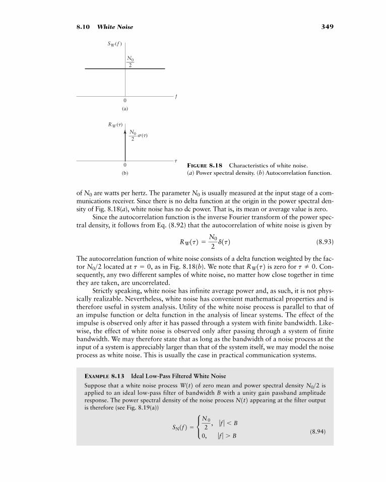
8.10 White Noise 349
of are watts per hertz. The parameter is usually measured at the input stage of a com-munications receiver. Since there is no delta function at the origin in the power spectral den-sity of Fig. 8.18(a), white noise has no dc power. That is, its mean or average value is zero.
Since the autocorrelation function is the inverse Fourier transform of the power spec-tral density, it follows from Eq. (8.92) that the autocorrelation of white noise is given by
(8.93)
The autocorrelation function of white noise consists of a delta function weighted by the fac-tor located at as in Fig. 8.18(b). We note that is zero for Con-sequently, any two different samples of white noise, no matter how close together in timethey are taken, are uncorrelated.
Strictly speaking, white noise has infinite average power and, as such, it is not phys-ically realizable. Nevertheless, white noise has convenient mathematical properties and istherefore useful in system analysis. Utility of the white noise process is parallel to that ofan impulse function or delta function in the analysis of linear systems. The effect of theimpulse is observed only after it has passed through a system with finite bandwidth. Like-wise, the effect of white noise is observed only after passing through a system of finitebandwidth. We may therefore state that as long as the bandwidth of a noise process at theinput of a system is appreciably larger than that of the system itself, we may model the noiseprocess as white noise. This is usually the case in practical communication systems.
EXAMPLE 8.13 Ideal Low-Pass Filtered White Noise
Suppose that a white noise process of zero mean and power spectral density isapplied to an ideal low-pass filter of bandwidth B with a unity gain passband amplituderesponse. The power spectral density of the noise process appearing at the filter outputis therefore (see Fig. 8.19(a))
(8.94)SN1f2 � c N0
2, ƒf ƒ � B
0, ƒf ƒ � B
N1t2N0>2W1t2
t 0.RW1t2t � 0,N0>2RW1t2 �
N0
2d1t2
N0N0
SW (f )
N0
2—–
N0
2—–
f
(a)
0
RW (�)
(�)
�
(b)
0 FIGURE 8.18 Characteristics of white noise. (a) Power spectral density. (b) Autocorrelation function.
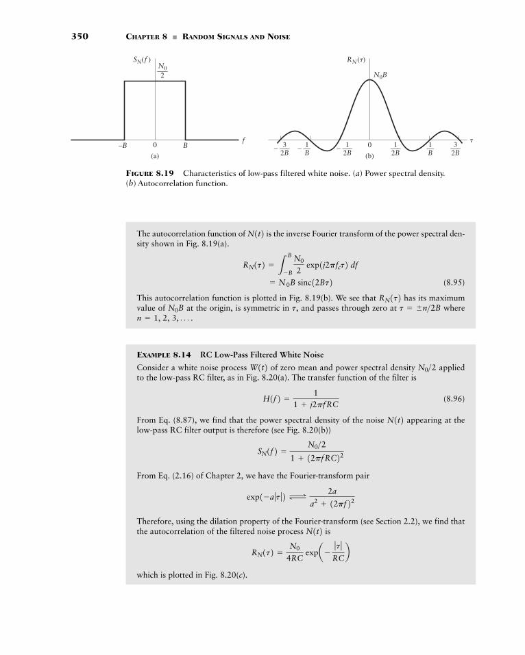
350 CHAPTER 8 � RANDOM SIGNALS AND NOISE
The autocorrelation function of is the inverse Fourier transform of the power spectral den-sity shown in Fig. 8.19(a).
(8.95)
This autocorrelation function is plotted in Fig. 8.19(b). We see that has its maximumvalue of at the origin, is symmetric in and passes through zero at where
EXAMPLE 8.14 RC Low-Pass Filtered White Noise
Consider a white noise process of zero mean and power spectral density appliedto the low-pass RC filter, as in Fig. 8.20(a). The transfer function of the filter is
(8.96)
From Eq. (8.87), we find that the power spectral density of the noise appearing at the low-pass RC filter output is therefore (see Fig. 8.20(b))
From Eq. (2.16) of Chapter 2, we have the Fourier-transform pair
Therefore, using the dilation property of the Fourier-transform (see Section 2.2), we find thatthe autocorrelation of the filtered noise process is
which is plotted in Fig. 8.20(c).
RN1t2 �N0
4RC expa�
ƒt ƒRCb
N1t2
exp1�a ƒt ƒ2 Δ2a
a2 12pf22
SN1f2 �N0>2
1 12pfRC22
N1t2H1f2 �
11 j2pfRC
N0>2W1t2
n � 1, 2, 3, Á .t � �n>2Bt,N0B
RN1t2� N0B sinc12Bt2
RN1t2 � LB
�B
N0
2 exp1j2pfct2 df
N1t2
SN(f )
f–B B
(a)
0
N0
2—–
RN(�)
�– —–
(b)
0
N0B
12B
—–12B
– —–32B
—–32B
– —1B
—1B
FIGURE 8.19 Characteristics of low-pass filtered white noise. (a) Power spectral density.(b) Autocorrelation function.
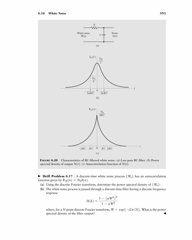
8.10 White Noise 351
� Drill Problem 8.17 A discrete-time white noise process has an autocorrelationfunction given by
(a) Using the discrete Fourier transform, determine the power spectral density of (b) The white noise process is passed through a discrete-time filter having a discrete-frequency
response
where, for a N-point discrete Fourier transform, What is the powerspectral density of the filter output? �
W � exp5�j2p>N6.H1k2 �
1 � 1aWk2N1 � aWk
5Wn6.RW1n2 � N0d1n2. 5Wn6
(b)
(a)
(c)
12�RC
SN(f )
f– —–—– 1
2�RC—–—–0
N0
2—–
N0
4—–
RN(�)
�–2RC 2RC–RC RC0
N0
4RC—–—
White noiseW(t)
NoiseN(t)C
R
FIGURE 8.20 Characteristics of RC-filtered white noise. (a) Low-pass RC filter. (b) Powerspectral density of output (c) Autocorrelation function of N1t2.N1t2.
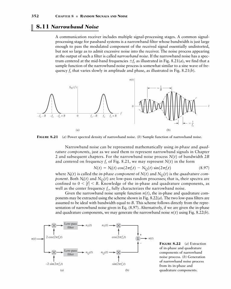
352 CHAPTER 8 � RANDOM SIGNALS AND NOISE
0 fc – B fc + Bfcf
t
– fc – B – fc + B– fc
0
�
n(t)
SN( f ) 1B
� 1fc
(a) (b)
FIGURE 8.21 (a) Power spectral density of narrowband noise. (b) Sample function of narrowband noise.
8.11 Narrowband Noise
A communication receiver includes multiple signal-processing stages. A common signal-processing stage for passband systems is a narrowband filter whose bandwidth is just largeenough to pass the modulated component of the received signal essentially undistorted,but not so large as to admit excessive noise into the receiver. The noise process appearingat the output of such a filter is called narrowband noise. If the narrowband noise has a spec-trum centered at the mid-band frequencies as illustrated in Fig. 8.21(a), we find that asample function of the narrowband noise process is somewhat similar to a sine wave of fre-quency that varies slowly in amplitude and phase, as illustrated in Fig. 8.21(b).fc
�fc
(a)
Low-passfilter
n(t)
n1(t)
nQ(t)
2 cos(2�fct)
–2 sin(2�fct)
Low-passfilter
(b)
Σ n(t)
n1(t)
nQ(t)
cos(2�fct)+
–
sin(2�fct)
FIGURE 8.22 (a) Extractionof in-phase and quadraturecomponents of narrowbandnoise process. (b) Generationof narrowband noise processfrom its in-phase andquadrature components.
Narrowband noise can be represented mathematically using in-phase and quad-rature components, just as we used them to represent narrowband signals in Chapter2 and subsequent chapters. For the narrowband noise process of bandwidth 2Band centered on frequency of Fig. 8.21, we may represent in the form
(8.97)
where is called the in-phase component of and is the quadrature com-ponent. Both and are low-pass random processes; that is, their spectra areconfined to Knowledge of the in-phase and quadrature components, aswell as the center frequency fully characterizes the narrowband noise.
Given the narrowband noise sample function the in-phase and quadrature com-ponents may be extracted using the scheme shown in Fig. 8.22(a). The two low-pass filters areassumed to be ideal with bandwidth equal to B. This scheme follows directly from the repre-sentation of narrowband noise given in Eq. (8.97). Alternatively, if we are given the in-phaseand quadrature components, we may generate the narrowband noise using Fig. 8.22(b).n1t2
n1t2,fc ,0 � ƒf ƒ � B.
NQ1t2NI1t2 NQ1t2N1t2NI1t2N1t2 � NI1t2 cos12pfct2 � NQ1t2 sin12pfct2
N1t2fcN1t2
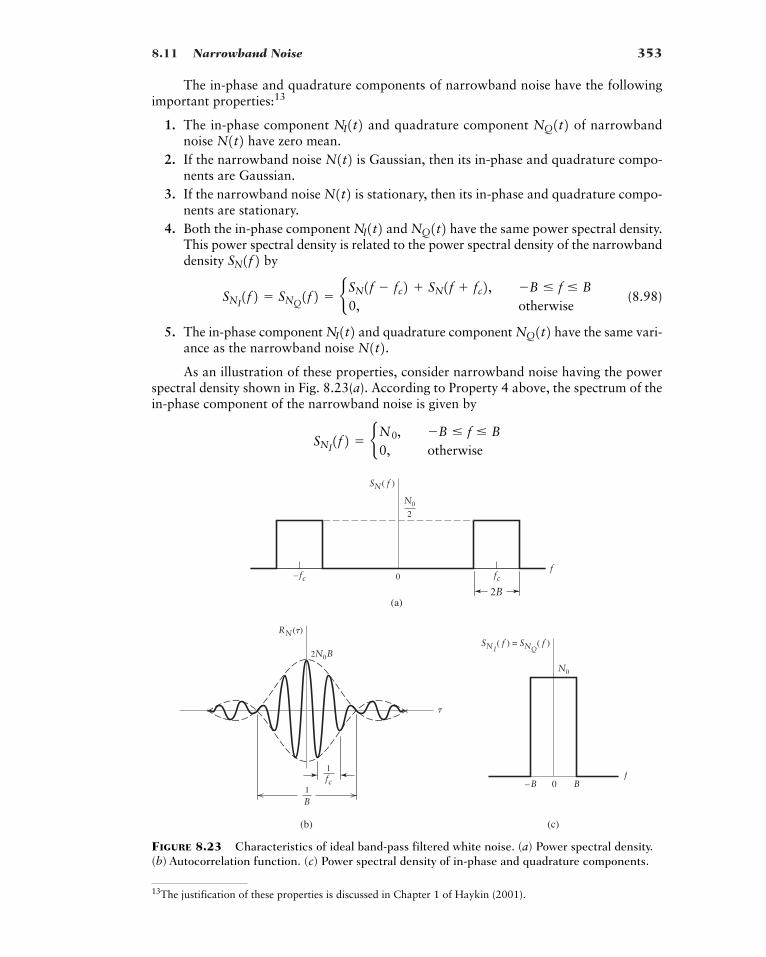
8.11 Narrowband Noise 353
13The justification of these properties is discussed in Chapter 1 of Haykin (2001).
The in-phase and quadrature components of narrowband noise have the followingimportant properties:13
1. The in-phase component and quadrature component of narrowbandnoise have zero mean.
2. If the narrowband noise is Gaussian, then its in-phase and quadrature compo-nents are Gaussian.
3. If the narrowband noise is stationary, then its in-phase and quadrature compo-nents are stationary.
4. Both the in-phase component and have the same power spectral density.This power spectral density is related to the power spectral density of the narrowbanddensity by
(8.98)
5. The in-phase component and quadrature component have the same vari-ance as the narrowband noise
As an illustration of these properties, consider narrowband noise having the powerspectral density shown in Fig. 8.23(a). According to Property 4 above, the spectrum of thein-phase component of the narrowband noise is given by
SNI1f2 � bN0, �B � f � B
0, otherwise
N1t2. NQ1t2NI1t2SNI1f2 � SNQ
1f2 � bSN1f � fc2 SN1f fc2, �B � f � B0, otherwise
SN1f2NQ1t2NI1t2
N1t2N1t2N1t2 NQ1t2NI1t2
2N0B
fcf
f
�
SN( f )
RN(�)
(a)2B
– fc
1fc
0
1B
N0
2
N0
(c)
SNI( f ) = SNQ
( f )
0 B–B
(b)
FIGURE 8.23 Characteristics of ideal band-pass filtered white noise. (a) Power spectral density.(b) Autocorrelation function. (c) Power spectral density of in-phase and quadrature components.
354 CHAPTER 8 � RANDOM SIGNALS AND NOISE
and the quadrature component has a similar spectrum. Thus the spectral density of the in-phase component is twice that of narrowband noise. However, since the narrowband noisehas nonzero spectral density in two bands of width 2B centered at we have that
which confirms Property 5 that the in-phase component has the same variance (power) asthe narrowband noise.
EXAMPLE 8.15 Ideal Band-Pass Filtered White Noise
Consider white Gaussian noise of zero mean and power spectral density which is passedthrough an ideal band-pass filter with center frequency bandwidth 2B, and passband mag-nitude response of unity. The power spectral density of the filtered white noise is then
(8.99)
as illustrated in Fig. 8.23(a). The problem is to determine the autocorrelation functions of and its in-phase and quadrature components.
The autocorrelation function of is the inverse Fourier transform of the power spec-tral density characteristic of Eq. (8.99), as shown by
(8.100)
This autocorrelation function of the ideal narrowband noise is plotted in Fig. 8.23(b).From Property 4 of narrowband noise, the in-phase and quadrature components have
an identical spectral density as shown in Fig. 8.23(c). The autocorrelation function of oris therefore (see Example 8.13)
(8.101)
� NOISE-EQUIVALENT BANDWIDTH
In Example 8.13, we observed that when a source of white noise of zero mean and powerspectral density is connected across the input of an ideal low-pass filter of bandwidthB and unity band-pass gain, the average output power (or equivalently ) is InExample 8.14, we observed that when a similar source is connected to a low-pass RC fil-ter, the corresponding average output power is For this filter, the 3-dB band-width is equal to We may therefore make two important observations. First,the filtered white noise has finite average power. Second, the average power is proportionalto bandwidth. We may generalize these observations to include all kinds of low-pass filtersby defining the noise-equivalent bandwidth as follows.
Suppose a white noise source with spectrum is connected to the inputof an arbitrary filter of transfer function From Properties 1 and 4 of power spectraldensities, the average output noise power is
H1f2. SW1f2 � N0>2
1>12pRC2. N0>14RC2.N0B.RN102N0>2
RNI1t2 � RNQ
1t2 � 2N0B sinc12Bt2NQ1t2 NI1t2
� 2N0B sinc12Bt2 cos12pfct2� N0B sinc12Bt23exp1�j2pfct2 exp12pfct24
RN1t2 � L�f
cB
�fc�B
N0
2 exp1j2pfct2 df L
fcB
fc�B
N0
2 exp1j2pfct2 df
n1t2N1t2
SN1f2 � cN0>2, ƒf � fc ƒ � BN0>2, ƒf fc ƒ � B0, otherwise
fc ,N0>2,
Lq
�qSN1f2 df � L
q
�qSNI1f2 df � 2N0B
�fc ,
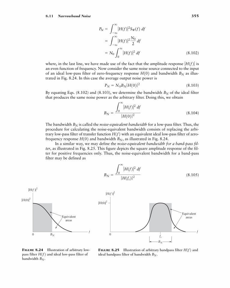
8.11 Narrowband Noise 355
(8.102)
where, in the last line, we have made use of the fact that the amplitude response isan even function of frequency. Now consider the same noise source connected to the inputof an ideal low-pass filter of zero-frequency response and bandwidth as illus-trated in Fig. 8.24. In this case the average output noise power is
(8.103)
By equating Eqs. (8.102) and (8.103), we determine the bandwidth of the ideal filterthat produces the same noise power as the arbitrary filter. Doing this, we obtain
(8.104)
The bandwidth is called the noise-equivalent bandwidth for a low-pass filter. Thus, theprocedure for calculating the noise-equivalent bandwidth consists of replacing the arbi-trary low-pass filter of transfer function with an equivalent ideal low-pass filter of zero-frequency response and bandwidth as illustrated in Fig. 8.24.
In a similar way, we may define the noise-equivalent bandwidth for a band-pass fil-ter, as illustrated in Fig. 8.25. This figure depicts the square amplitude response of the fil-ter for positive frequencies only. Thus, the noise-equivalent bandwidth for a band-passfilter may be defined as
(8.105)BN �L
q
0ƒH1f2 ƒ2 df
ƒH1fc2 ƒ 2
BN ,H102 H1f2BN
BN �L
q
0ƒH1f2 ƒ2 df
ƒH102 ƒ 2
BN
PN � N0BN ƒH102 ƒ 2BNH102
ƒH1f2 ƒ� N0L
q
0ƒH1f2 ƒ2 df
� Lq
�qƒH1f2 ƒ2 N0
2df
PN � Lq
�qƒH1f2 ƒ2SW1f2 df
BN0
Equivalentareas
|H(f )|2
|H(0)|2
f
BN
Equivalentareas
|H(f )|2
|H(0)|2
f0 fc
FIGURE 8.25 Illustration of arbitrary bandpass filter andideal bandpass filter of bandwidth BN .
H1f2FIGURE 8.24 Illustration of arbitrary low-pass filter and ideal low-pass filter ofbandwidth BN .
H1f2
356 CHAPTER 8 � RANDOM SIGNALS AND NOISE
where is the center-frequency amplitude response of the filter. In fact, we recognizethat Eq. (8.105) may be used to represent both cases by setting for low-pass filters.Then we have the general result
(8.106)
and the effect of passing white noise through a filter may be separated into two parts:
� The center-frequency power gain
� The noise equivalent bandwidth representing the frequency selectivity of the filter.
This separation applies whether the filter is low-pass or band-pass. Hence, as a general rule wemay say that effect of noise in the system is reduced by narrowing the system bandwidth.
EXAMPLE 8.16 Noise Equivalent Bandwidth of RC Filter
Consider the single-pole low-pass filter of Example 8.14. The transfer function of this filter is
We wish to find the noise equivalent bandwidth of this filter.The noise equivalent bandwidth of this filter is
Recognizing the integrand as the scaled derivative of we obtain
Due to the slow roll-off of the single-pole filter, the noise bandwidth is slightly larger than its3-dB bandwidth,
8.12 Summary and Discussion
We began this chapter by indicating that information and noise are both random signals;indeed, it is this randomness or unpredictability that is a key property of communicationsystems. However, even random signals have statistical characteristics that may be measured.We subsequently presented several important tools for characterizing random signals.
We introduced a random experiment as a model for unpredictable phenomena; and therelative frequency definition of probability as a means of assigning a likelihood to the out-come of a random experiment. This led to the three basic axioms of probability theory.
B3dB � 1>12pRC2.
�1
4RC
�1
2pRCap
2� 0b
BN �1
2pRCtan�112pfRC2 `
0
q
tan�11f2,� 1 L
�
0
df
1 12pfRC22
BN �1
ƒH102 ƒ2 Lq
0ƒH1f2 ƒ2 df
H1f2 �1
1 j2pfRC
BN ,
ƒH1fc2 ƒ2.
PN � N0 ƒH1fc2 ƒ2BN
fc � 0ƒH1fc2 ƒ2
Additional Problems 357
Random variables were introduced as a function whose domain is the sample spaceof the random experiment and whose range is the real numbers. Random variables providea method to unify the treatment of a wide variety of random experiments. Probability dis-tribution and density functions were shown as fundamental methods of characterizing a ran-dom variable.
The study of functions of random variables led naturally to the concept of expecta-tion and the statistical moments and covariance of random variables.
Gaussian random variables were introduced as a particular important type of randomvariable in the study of communication systems.
Considering time as parameter in random signals led to the study of random processes.A random process was defined as a family of random variables indexed by time as a para-meter. Stationary, ergodic, and wide-sense stationary random processes were introduced asmodels of most physical processes exhibiting random behavior. It was shown that wide-sensestationary random processes have many of the properties of deterministic power signals,including the fact that the Weiner–Khintchine formulas relate the spectrum of the randomprocess to its autocorrelation.
Gaussian processes and white noise were introduced as important random processesin the analysis of communication systems.
Finally, it was shown that, similar to deterministic signals, we may consider bandpassor narrowband versions of noise. This narrowband noise has in-phase and quadraturecomponents, similar to deterministic signals.
This chapter has been a brief and certainly not complete introduction to the ran-dom signals and noise that are commonly found in communication systems, but the treat-ment presented herein is adequate for an introductory treatment of statisticalcommunication theory. The two subsequent chapters will illustrate the importance ofthe material presented in this chapter in designing receivers and evaluating communica-tion system performance.
ADDITIONAL PROBLEMS
8.18 Consider a deck of 52 cards, divided into four different suits, with 13 cards in each suit rang-ing from the two up through the ace. Assume that all the cards are equally likely to be drawn.(a) Suppose that a single card is drawn from a full deck. What is the probability that this card
is the ace of diamonds? What is the probability that the single card drawn is an ace of anyone of the four suits?
(b) Suppose that two cards are drawn from the full deck. What is the probability that the cardsdrawn are an ace and a king, not necessarily the same suit? What if they are of the same suit?
8.19 Suppose a player has one red die and one white die. How many outcomes are possible in therandom experiment of tossing the two dice? Suppose the dice are indistinguishable, how manyoutcomes are possible?
8.20 Refer to Problem 8.19.
(a) What is the probability of throwing a red 5 and a white 2?
(b) If the dice are indistinguishable, what is the probability of throwing a sum of 7? If they aredistinguishable, what is this probability?
8.21 Consider a random variable X that is uniformly distributed between the values of 0 and1 with probability takes on the value 1 with probability and is uniformly distributedbetween values 1 and 2 with probability Determine the distribution function of the ran-dom variable X.
12 .
14 ,1
4 ,
358 CHAPTER 8 � RANDOM SIGNALS AND NOISE
8.22 Consider a random variable X defined by the double-exponential density
where a and b are constants.
(a) Determine the relationship between a and b so that is a probability density function.
(b) Determine the corresponding distribution function
(c) Find the probability that the random variable X lies between 1 and 2.
8.23 Show that the expression for the variance of a random variable can be expressed in terms of thefirst and second moments as
8.24 A random variable R is Rayleigh distributed with its probability density function given by
(a) Determine the corresponding distribution function
(b) Show that the mean of R is equal to
(c) What is the mean-square value of R?
(d) What is the variance of R?
8.25 Consider a uniformly distributed random variable Z, defined by
The two random variables X and Y are related to Z by and
(a) Determine the probability density functions of X and Y.
(b) Show that X and Y are uncorrelated random variables.
(c) Are X and Y statistically independent? Why?
8.26 A Gaussian random variable has zero mean and a standard deviation of 10 V. A constant volt-age of 5 V is added to this random variable.
(a) Determine the probability that a measurement of this composite signal yields a positive value.
(b) Determine the probability that the arithmetic mean of two independent measurements of thissignal is positive.
8.27 Consider a random process defined by
in which the frequency W is a random variable with the probability density function
Show that is nonstationary.8.28 Consider the sinusoidal process
X1t2 � A cos12pfct2X1t2
fW1w2 � c 1B
, 0 � w � B
0, otherwise
X1t2 � sin12pWt2X1t2
Y � cos1Z2.X � sin1Z2fZ1z2 � c 1
2p, 0 � z � 2p
0, otherwise
2bp>2 .
FR1r2.fR1r2 � c r
b exp¢�
r2
2b≤ , 0 � r � �
0, otherwise
Var1X2 � E3X24 � E3X42
FX1x2.fX1x2
fX1x2 � a exp1�b ƒx ƒ2, �� � x � �
Additional Problems 359
where the frequency is constant and the amplitude A is uniformly distributed:
Determine whether or not this process is stationary in the strict sense.8.29 A random process is defined by
where A is a Gaussian random variable of zero mean and variance This random process isapplied to an ideal integrator, producing an output defined by
(a) Determine the probability density function of the output at a particular time (b) Determine whether or not is stationary.
8.30 Prove the following two properties of the autocorrelation function of a random process
(a) If contains a dc component equal to A, then contains a constant componentequal to
(b) If contains a sinusoidal component, then also contains a sinusoidal compo-nent of the same frequency.
8.31 A discrete-time random process is defined by
where the zero-mean random process is stationary with autocorrelation functionWhat is the autocorrelation function a wide-sense sta-
tionary process? Justify your answer.8.32 Find the power spectral density of the process that has the autocorrelation function
8.33 A random pulse has amplitude A and duration T but starts at an arbitrary time That is, therandom process is defined as
where rect(t) is defined in Section 2.9. The random variable is assumed to be uniformly dis-tributed over with density
(a) What is the autocorrelation function of the random process (b) What is the spectrum of the random process
8.34 Given that a stationary random process has an autocorrelation function and apower spectral density show that:(a) The autocorrelation function of the first derivative of , is equal to the neg-
ative of the second derivative of (b) The power spectral density of is equal to
Hint: See the solution to problem 2.244p2f 2SX1f2.dX1t2>dt,
RX1t2. X1t2dx1t2>dt,SX1f2, RX1t2X1t2 X1t2? X1t2?
ft01s2 � c 1T
, 0 � s � T
0, otherwise
30, T4 t0
X1t2 � A rect1t t02t0 .
RX1t2 � bs211 � ƒt ƒ2, for ƒt ƒ � 10, for ƒt ƒ � 1
Ry(k) of Yn? Is YnRW(k) � s2d(k).5Wn6
Yn � aYn Wn, n � Á , �1, 0, 1, Á
5Yn6RX1t2X1t2 A2.
RX1t2X1t2X1t2: RX1t2Y1t2 tk .Y1t2
Y1t2 � Lt
0X1t2 dt
Y1t2 sA2 .
X1t2 � A cos12pfct2X1t2
fA1a2 � b 1, 0 � a � 10, otherwise
fc
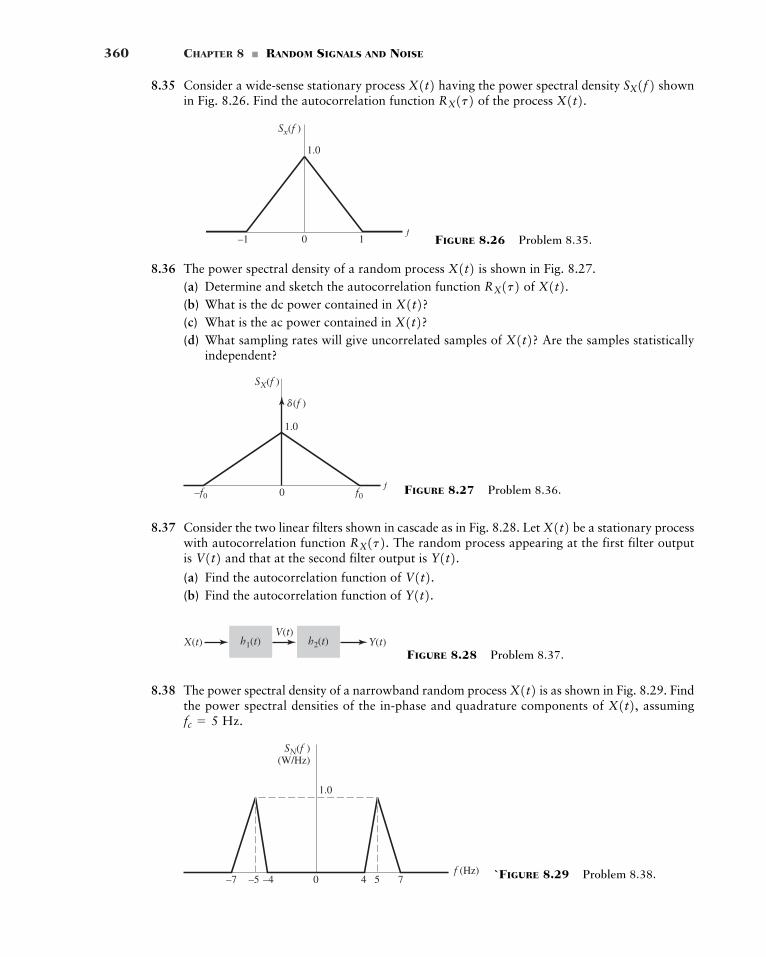
360 CHAPTER 8 � RANDOM SIGNALS AND NOISE
8.35 Consider a wide-sense stationary process having the power spectral density shownin Fig. 8.26. Find the autocorrelation function of the process X1t2.RX1t2 SX1f2X1t2
1.0
Sx(f )
0f
–1 1 FIGURE 8.26 Problem 8.35.
8.36 The power spectral density of a random process is shown in Fig. 8.27.(a) Determine and sketch the autocorrelation function of (b) What is the dc power contained in (c) What is the ac power contained in (d) What sampling rates will give uncorrelated samples of Are the samples statistically
independent?X1t2?X1t2?X1t2? X1t2.RX1t2
X1t2
1.0
�(f )
SX(f )
0f
–f0 f0
8.37 Consider the two linear filters shown in cascade as in Fig. 8.28. Let be a stationary processwith autocorrelation function The random process appearing at the first filter outputis and that at the second filter output is
(a) Find the autocorrelation function of (b) Find the autocorrelation function of Y1t2.V1t2.
Y1t2.V1t2 RX1t2. X1t2
h1(t)V(t)
h2(t)X(t) Y(t)FIGURE 8.28 Problem 8.37.
SN(f )(W/Hz)
f (Hz)0
1.0
4 5 7–7 –5 –4
8.38 The power spectral density of a narrowband random process is as shown in Fig. 8.29. Findthe power spectral densities of the in-phase and quadrature components of assumingfc � 5 Hz.
X1t2,X1t2
FIGURE 8.27 Problem 8.36.
`FIGURE 8.29 Problem 8.38.
Advanced Problems 361
8.39 Assume the narrowband process described in Problem 8.38 is Gaussian with zero meanand variance
(a) Calculate(b) Determine the joint probability density function of the random variables Y and Z obtained
by observing the in-phase and quadrature components of at some fixed time.
ADVANCED PROBLEMS
8.40 Find the probability that the last two digits of the cube of a natural number willbe 01.
8.41 Consider the random experiment of selecting a number uniformly distributed over the rangeLet A, B, and C be the events that the selected number is a multiple of 3,
4, and 6, respectively.(a) What is the probability of event A—that is, P[A]?
(b) What is ?
(c) What is
(d) What is
(e) What is 8.42 A message consists of ten 0s and 1s.
(a) How many such messages are there?(b) How many such messages are there that contain exactly four 1s?(c) Suppose the 10th bit is not independent of the others but is chosen such that the modulo-
2 sum of all the bits is zero. This is referred to as an even-parity sequence. How many sucheven-parity sequences are there?
(d) If this ten-bit even-parity sequence is transmitted over a channel that has a probability oferror p for each bit. What is the probability that the received sequence contains an unde-tected error?
8.43 The probability that an event occurs at least once in four independent trials is equal to 0.59. Whatis the probability of occurrence of the event in one trial, if the probabilities are equal in all trials?
8.44 The arrival times of two signals at a receiver are uniformly distributed over the interval The receiver will be jammed if the time difference in the arrivals is less than Find the proba-bility that the receiver will be jammed.
8.45 A telegraph system (an early version of digital communications) transmits either a dot or dashsignal. Assume the transmission properties are such that of the dots and of the dashesare received incorrectly. Suppose the ratio of transmitted dots to transmitted dashes is 5 to 3.What is the probability that a received signal is as transmitted if:(a) The received signal is a dot?(b) The received signal is a dash?
8.46 Four radio signals are emitted successively. The probability of reception for each of them isindependent of the reception of the others and equal, respectively, 0.1, 0.2, 0.3, and 0.4. Findthe probability that k signals will be received where
8.47 In a computer-communication network, the arrival time between messages is modeled withan exponential distribution function having the density
fT1t2 � c 1l
e�lt, t � 0
0, otherwise
t
k � 1, 2, 3, 4.
1>32>5
t.30, T4.
P3A ∩ C4?P3A ∪ B4?P3A ∩ B4?P3B4?
51, 2, 3, Á , 1206.
11, 2, 3, Á 2
X1t2sX
2 .
sX2 .
X1t2
362 CHAPTER 8 � RANDOM SIGNALS AND NOISE
(a) What is the mean time between messages with this distribution?(b) What is the variance in this time between messages?
8.48 If X has a density find the density of the random variable Y defined as follows:(a) for constants a and b.(b)(c) assuming X is a nonnegative random variable.
8.49 Let X and Y be two independent random variables with density functions and respectively. Show that the random variable has a density function given by
Hint:
8.50 Find the spectral density if
where and are independent zero-mean random processes with
8.51 Consider a random process defined by
where the frequency is a random variable uniformly distributed over the interval [0, W].Show that is nonstationary. Hint: Examine specific sample functions of the random process
for, say, the frequencies and W.8.52 The oscillators used in communication systems are not ideal but often suffer from a distortion
known as phase noise. Such an oscillator may be modeled by the random process
where is a slowly varying random process. Describe and justify the conditions on the ran-dom process such that is wide-sense stationary.
8.53 A baseband signal is disturbed by an additive noise process as shown by
where is a stationary Gaussian process of zero mean and variance (a) Determine the density functions of the random variables and where
(b) The noise process has an autocorrelation function given by
Determine the joint density function of and , that is, fX1, X2
(x1, x2).X2X1
RN (t) � s2 exp1� ƒ t ƒ 2N1t2
X2 � X(t) ƒ t�2
X1 � X(t) ƒ t�1
X2X1
s2 .N1t2
X1t2 � A sin10.3pt2 N(t)
N1t2Y1t2f(t)f(t)
Y1t2 � A cos12pfct f(t)2
W>2,W>4,X1t2 X1t2 fc
X1t2 � sin12pfct2X1t2RX1t2 � a1e�a1 ƒt ƒ, and RY1t2 � a2e�a2 ƒt ƒ.
Y1t2X1t2Z1t2 � X1t2 Y1t2
SZ1f2P[Z � z] � P[X � z, Y � z � X]
fZ1z2 � L0
��fY1z � s2 fX1s2ds
Z � X YfY1x2,fX1x2
Y � 2X ,Y � X2.Y � aX b
fX1x2,
Computer Experiments 363
� COMPUTER EXPERIMENTS
8.54 For this die-tossing experiment, a MATLAB script is included in Appendix 7. The MATLABscript simulates the tossing of a biased die 1000 times. The steps to the script are:
� Roll the die N times and save the results in X.� Compute a histogram on X to obtain the probabilities of the different faces.
Repeat the experiment for 100, 1000, and 10,000. Comment on the relative frequencydefinition of probability as a function of N, the number of throws.
8.55 To demonstrate the central limit theorem, we compute 20,000 samples of Z for and esti-mate the corresponding probability density function by forming a histogram of the results. AMATLAB script for performing this is included in Appendix 7. Compare this histogram (scaledfor unit area) to the Gaussian density function having the same mean and variance.
8.56 Revise the script for Problem 8.55 to find the distribution of a sum of Bernoulli random vari-ables. Compare it to the Gaussian distribution as N becomes large.
8.57 Revise the script for Problem 8.55 so the mean values are not identical but have a random dis-tribution as well, but with the same overall mean. Compute the distribution of the sum.
8.58 In this computer experiment, we will simulate a Gaussian random process digitally. A MATLABscript in Appendix 7 generates a discrete-time white Gaussian process and filters it with a dis-crete-time root-raised cosine filter (as discussed in Chapter 6). In the script, we perform the fol-lowing steps:
• Generate a discrete-time white Gaussian process.• Filter this Gaussian process with a root-raised cosine filter having 25 percent excess
bandwidth.
• Compute the spectrum of the resulting discrete-time process.• Compute the autocorrelation of the resulting discrete-time process.
(a) Determine the autocorrelation of the filtered sequence.(b) Determine the spectrum of the filtered sequence.
Comment on the results.
N � 5,
N � 10,
364
1In this chapter and the following, we use lowercase letters for random signals with the understanding that they represent samplefunctions of the underlying random processes.
CHAPTER 9
NOISE IN ANALOG
COMMUNICATIONS
In this chapter, we revisit the analog modulation methods of Chapters 3 and 4 in light ofthe noise-related concepts introduced in Chapter 8. In practice, we find that modulatedsignals, regardless of their kind, are perturbed by noise and by the imperfect characteristicsof the channel during transmission. Noise can broadly be defined as any unknown signalthat affects the recovery of the desired signal. There may be many sources of noise in acommunication system, but often the major sources are the communication devices them-selves or interference encountered during the course of transmission. There are severalways that noise can affect the desired signal, but one of the most common ways is as anadditive distortion. That is, the received signal is modeled as1
(9.1)
where is the transmitted signal and is the additive noise. If we knew the noiseexactly, then we could subtract it from and recover the transmitted signal exactly.Unfortunately, this is rarely the case. Much of communication system design is related toprocessing the received signal in a manner that minimizes the effect of additive noise.
This chapter will focus on the detection of analog signals in the presence of additivenoise. The material in this chapter teaches us the following lessons.
� Lesson 1: Minimizing the effects of noise is a prime concern in analog communications,and consequently the ratio of signal power to noise power is an important metric forassessing analog communication quality.
� Lesson 2: Amplitude modulation may be detected either coherently requiring the use ofa synchronized oscillator or non-coherently by means of a simple envelope detector.However, there is a performance penalty to be paid for non-coherent detection.
� Lesson 3: Frequency modulation is nonlinear and the output noise spectrum is parabolicwhen the input noise spectrum is flat. Frequency modulation has the advantage that itallows us to trade bandwidth for improved performance.
� Lesson 4: Pre- and de-emphasis filtering is a method of reducing the output noise of anFM demodulator without distorting the signal. This technique may be used to significantlyimprove the performance of frequency modulation systems.
r1t2r1t2w1t2s1t2
r1t2 � s1t2 w1t2
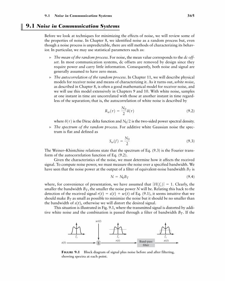
9.1 Noise in Communication Systems 365
Band-passfilter
Σs(t)r(t) x(t)
w(t)
fc fc fc
FIGURE 9.1 Block diagram of signal plus noise before and after filtering,showing spectra at each point.
9.1 Noise in Communication Systems
Before we look at techniques for minimizing the effects of noise, we will review some ofthe properties of noise. In Chapter 8, we identified noise as a random process but, eventhough a noise process is unpredictable, there are still methods of characterizing its behav-ior. In particular, we may use statistical parameters such as:
� The mean of the random process. For noise, the mean value corresponds to the dc off-set. In most communication systems, dc offsets are removed by design since theyrequire power and carry little information. Consequently, both noise and signal aregenerally assumed to have zero mean.
� The autocorrelation of the random process. In Chapter 11, we will describe physicalmodels for receiver noise and means of characterizing it. As it turns out, white noise,as described in Chapter 8, is often a good mathematical model for receiver noise, andwe will use this model extensively in Chapters 9 and 10. With white noise, samplesat one instant in time are uncorrelated with those at another instant in time regard-less of the separation; that is, the autocorrelation of white noise is described by
(9.2)
where is the Dirac delta function and is the two-sided power spectral density.
� The spectrum of the random process. For additive white Gaussian noise the spec-trum is flat and defined as
(9.3)
The Weiner–Khintchine relations state that the spectrum of Eq. (9.3) is the Fourier trans-form of the autocorrelation function of Eq. (9.2).
Given the characteristics of the noise, we must determine how it affects the receivedsignal. To compute noise power, we must measure the noise over a specified bandwidth. Wehave seen that the noise power at the output of a filter of equivalent-noise bandwidth is
(9.4)
where, for convenience of presentation, we have assumed that Clearly, thesmaller the bandwidth the smaller the noise power N will be. Relating this back to thedetection of the received signal of Eq. (9.1), it seems intuitive that weshould make as small as possible to minimize the noise but it should be no smaller thanthe bandwidth of otherwise we will distort the desired signal.
This situation is illustrated in Fig. 9.1, where the transmitted signal is distorted by addi-tive white noise and the combination is passed through a filter of bandwidth If theBT .
s1t2,BT
r1t2 � s1t2 w1t2BT ,ƒH1fc2 ƒ � 1.
N � N0BT
BT
Sw1f2 �N0
2
N0>2d1t2Rw1t2 �
N0
2d1t2
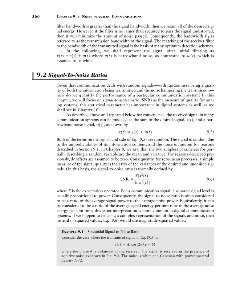
366 CHAPTER 9 � NOISE IN ANALOG COMMUNICATIONS
filter bandwidth is greater than the signal bandwidth, then we retain all of the desired sig-nal energy. However, if the filter is no larger than required to pass the signal undistorted,then it will minimize the amount of noise passed. Consequently, the bandwidth isreferred to as the transmission bandwidth of the signal. The matching of the receiver filterto the bandwidth of the transmitted signal is the basis of many optimum detection schemes.
In the following, we shall represent the signal after initial filtering aswhere is narrowband noise, as contrasted to which is
assumed to be white.
9.2 Signal-To-Noise Ratios
Given that communication deals with random signals—with randomness being a qual-ity of both the information being transmitted and the noise hampering the transmission—how do we quantify the performance of a particular communication system? In thischapter, we will focus on signal-to-noise ratio (SNR) as the measure of quality for ana-log systems; this statistical parameter has importance in digital systems as well, as weshall see in Chapter 10.
As described above and repeated below for convenience, the received signal in manycommunication systems can be modeled as the sum of the desired signal, and a nar-rowband noise signal, as shown by
(9.5)
Both of the terms on the right-hand side of Eq. (9.5) are random. The signal is random dueto the unpredictability of its information content, and the noise is random for reasonsdescribed in Section 9.1. In Chapter 8, we saw that the two simplest parameters for par-tially describing a random variable are the mean and variance. For reasons described pre-viously, dc offsets are assumed to be zero. Consequently, for zero-mean processes, a simplemeasure of the signal quality is the ratio of the variances of the desired and undesired sig-nals. On this basis, the signal-to-noise ratio is formally defined by
(9.6)
where E is the expectation operator. For a communication signal, a squared signal level isusually proportional to power. Consequently, the signal-to-noise ratio is often consideredto be a ratio of the average signal power to the average noise power. Equivalently, it canbe considered to be a ratio of the average signal energy per unit time to the average noiseenergy per unit time; this latter interpretation is more common in digital communicationsystems. If we happen to be using a complex representation of the signals and noise, theninstead of squared values, Eq. (9.6) would use magnitude-squared values.
EXAMPLE 9.1 Sinusoidal Signal-to-Noise Ratio
Consider the case where the transmitted signal in Eq. (9.5) is
where the phase is unknown at the receiver. The signal is received in the presence ofadditive noise as shown in Fig. 9.2. The noise is white and Gaussian with power spectraldensity N0>2.
u
s1t2 � Ac cos12pfct u2
SNR �E3s21t24E3n21t24
x1t2 � s1t2 n1t2n1t2, s1t2,
w1t2,n1t2x1t2 � s1t2 n1t2
BT
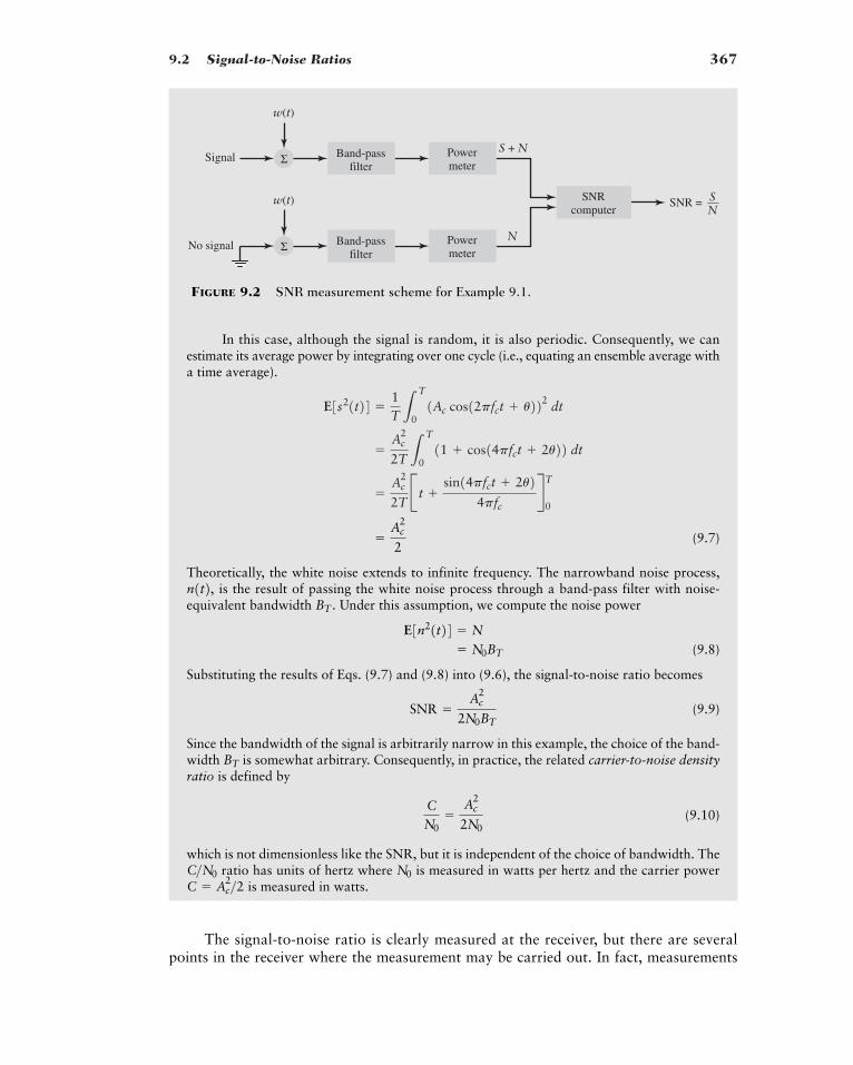
9.2 Signal-to-Noise Ratios 367
Σ
w(t)
Signal
No signal
Band-passfilter
Powermeter
Σ
w(t)
N
S + N
SNR = —SN
Band-passfilter
Powermeter
SNRcomputer
FIGURE 9.2 SNR measurement scheme for Example 9.1.
In this case, although the signal is random, it is also periodic. Consequently, we canestimate its average power by integrating over one cycle (i.e., equating an ensemble average witha time average).
(9.7)
Theoretically, the white noise extends to infinite frequency. The narrowband noise process,is the result of passing the white noise process through a band-pass filter with noise-
equivalent bandwidth Under this assumption, we compute the noise power
(9.8)
Substituting the results of Eqs. (9.7) and (9.8) into (9.6), the signal-to-noise ratio becomes
(9.9)
Since the bandwidth of the signal is arbitrarily narrow in this example, the choice of the band-width is somewhat arbitrary. Consequently, in practice, the related carrier-to-noise densityratio is defined by
(9.10)
which is not dimensionless like the SNR, but it is independent of the choice of bandwidth. Theratio has units of hertz where is measured in watts per hertz and the carrier power
is measured in watts.
The signal-to-noise ratio is clearly measured at the receiver, but there are severalpoints in the receiver where the measurement may be carried out. In fact, measurements
C � Ac2>2 N0C>N0
CN0
�Ac
2
2N0
BT
SNR �Ac
2
2N0BT
� N0BT
E3n21t24 � N
BT .n1t2,
�Ac
2
2
�Ac
2
2TB t
sin14pfct 2u24pfc
R0
T
�Ac
2
2T LT
011 cos14pfct 2u22 dt
E3s21t24 �1T L
T
01Ac cos12pfct u222 dt
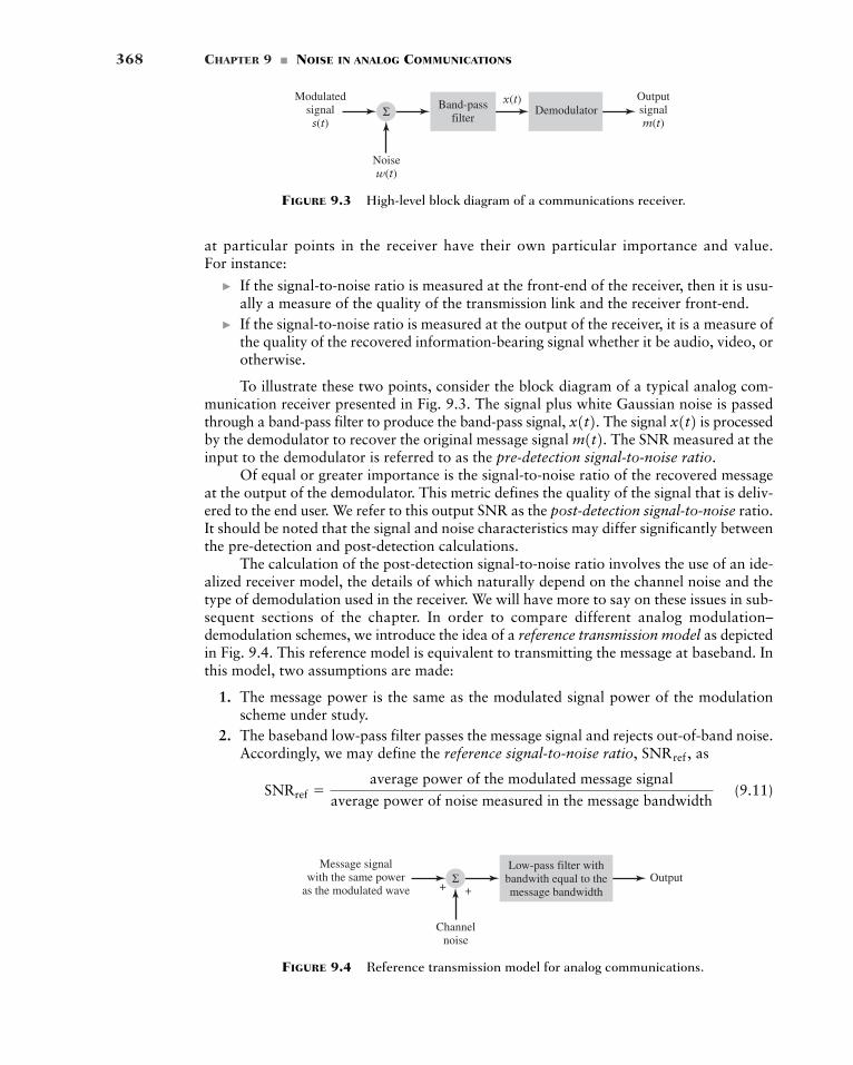
368 CHAPTER 9 � NOISE IN ANALOG COMMUNICATIONS
Modulatedsignals(t)
Outputsignalm(t)
x(t)Band-passfilter
Demodulator
Noisew(t)
Σ
FIGURE 9.3 High-level block diagram of a communications receiver.
OutputMessage signal
with the same poweras the modulated wave
Low-pass filter withbandwith equal to themessage bandwidth
Channelnoise
++Σ
at particular points in the receiver have their own particular importance and value. For instance:
� If the signal-to-noise ratio is measured at the front-end of the receiver, then it is usu-ally a measure of the quality of the transmission link and the receiver front-end.
� If the signal-to-noise ratio is measured at the output of the receiver, it is a measure ofthe quality of the recovered information-bearing signal whether it be audio, video, orotherwise.
To illustrate these two points, consider the block diagram of a typical analog com-munication receiver presented in Fig. 9.3. The signal plus white Gaussian noise is passedthrough a band-pass filter to produce the band-pass signal, The signal is processedby the demodulator to recover the original message signal The SNR measured at theinput to the demodulator is referred to as the pre-detection signal-to-noise ratio.
Of equal or greater importance is the signal-to-noise ratio of the recovered messageat the output of the demodulator. This metric defines the quality of the signal that is deliv-ered to the end user. We refer to this output SNR as the post-detection signal-to-noise ratio.It should be noted that the signal and noise characteristics may differ significantly betweenthe pre-detection and post-detection calculations.
The calculation of the post-detection signal-to-noise ratio involves the use of an ide-alized receiver model, the details of which naturally depend on the channel noise and thetype of demodulation used in the receiver. We will have more to say on these issues in sub-sequent sections of the chapter. In order to compare different analog modulation–demodulation schemes, we introduce the idea of a reference transmission model as depictedin Fig. 9.4. This reference model is equivalent to transmitting the message at baseband. Inthis model, two assumptions are made:
1. The message power is the same as the modulated signal power of the modulationscheme under study.
2. The baseband low-pass filter passes the message signal and rejects out-of-band noise.Accordingly, we may define the reference signal-to-noise ratio, as
(9.11)SNRref �average power of the modulated message signal
average power of noise measured in the message bandwidth
SNRref ,
m1t2. x1t2x1t2.
FIGURE 9.4 Reference transmission model for analog communications.
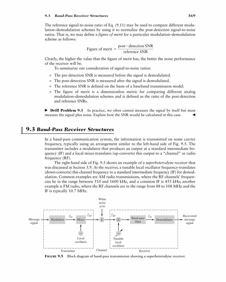
9.3 Band-Pass Receiver Structures 369
The reference signal-to-noise ratio of Eq. (9.11) may be used to compare different modu-lation–demodulation schemes by using it to normalize the post-detection signal-to-noiseratios. That is, we may define a figure of merit for a particular modulation–demodulationscheme as follows:
Clearly, the higher the value that the figure of merit has, the better the noise performanceof the receiver will be.
To summarize our consideration of signal-to-noise ratios:
� The pre-detection SNR is measured before the signal is demodulated.� The post-detection SNR is measured after the signal is demodulated.� The reference SNR is defined on the basis of a baseband transmission model.� The figure of merit is a dimensionless metric for comparing different analog
modulation–demodulation schemes and is defined as the ratio of the post-detectionand reference SNRs.
� Drill Problem 9.1 In practice, we often cannot measure the signal by itself but mustmeasure the signal plus noise. Explain how the SNR would be calculated in this case. �
9.3 Band-Pass Receiver Structures
In a band-pass communication system, the information is transmitted on some carrierfrequency, typically using an arrangement similar to the left-hand side of Fig. 9.5. Thetransmitter includes a modulator that produces an output at a standard intermediate fre-quency (IF) and a local mixer-translates (up-converts) this output to a “channel” or radiofrequency (RF).
The right-hand side of Fig. 9.5 shows an example of a superheterodyne receiver thatwas discussed in Section 3.9. At the receiver, a tunable local oscillator frequency-translates(down-converts) this channel frequency to a standard intermediate frequency (IF) for demod-ulation. Common examples are AM radio transmissions, where the RF channels’ frequen-cies lie in the range between 510 and 1600 kHz, and a common IF is 455 kHz; anotherexample is FM radio, where the RF channels are in the range from 88 to 108 MHz and theIF is typically 10.7 MHz.
Figure of merit �post�detection SNR
reference SNR
FIGURE 9.5 Block diagram of band-pass transmission showing a superheterodyne receiver.
Messagesignal
Recoveredmessagesignal
Modulator Band-passfilter
Mixer Demodulator
Localoscillator
Transmitter ReceiverChannel
Tunablelocal
oscillator
Whitenoisew(t)
fRF fRFfIF fIFΣ
~ ~
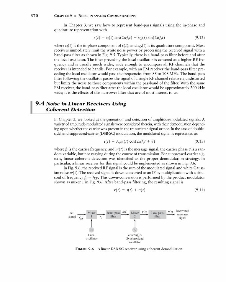
370 CHAPTER 9 � NOISE IN ANALOG COMMUNICATIONS
Recoveredmessagesignal
Localoscillator
cos(2�fc t)Synchronized
oscillator
RFsignal
x(t) v(t) y(t)Low-passfilter
Mixer1
Mixer2
Band-passfilterfRF
fc
~ ~
FIGURE 9.6 A linear DSB-SC receiver using coherent demodulation.
In Chapter 3, we saw how to represent band-pass signals using the in-phase andquadrature representation with
(9.12)
where is the in-phase component of and is its quadrature component. Mostreceivers immediately limit the white noise power by processing the received signal with aband-pass filter as shown in Fig. 9.5. Typically, there is a band-pass filter before and afterthe local oscillator. The filter preceding the local oscillator is centered at a higher RF fre-quency and is usually much wider, wide enough to encompass all RF channels that thereceiver is intended to handle. For example, with an FM receiver the band-pass filter pre-ceding the local oscillator would pass the frequencies from 88 to 108 MHz. The band-passfilter following the oscillator passes the signal of a single RF channel relatively undistortedbut limits the noise to those components within the passband of the filter. With the sameFM receiver, the band-pass filter after the local oscillator would be approximately 200 kHzwide; it is the effects of this narrower filter that are of most interest to us.
9.4 Noise in Linear Receivers UsingCoherent Detection
In Chapter 3, we looked at the generation and detection of amplitude-modulated signals. Avariety of amplitude-modulated signals were considered therein, with their demodulation depend-ing upon whether the carrier was present in the transmitter signal or not. In the case of double-sideband suppressed-carrier (DSB-SC) modulation, the modulated signal is represented as
(9.13)
where is the carrier frequency, and is the message signal; the carrier phase is a ran-dom variable, but not varying during the course of transmission. For suppressed-carrier sig-nals, linear coherent detection was identified as the proper demodulation strategy. Inparticular, a linear receiver for this signal could be implemented as shown in Fig. 9.6.
In Fig. 9.6, the received RF signal is the sum of the modulated signal and white Gauss-ian noise The received signal is down-converted to an IF by multiplication with a sinu-soid of frequency This down-conversion is performed by the product modulatorshown as mixer 1 in Fig. 9.6. After band-pass filtering, the resulting signal is
(9.14)x1t2 � s1t2 n1t2fc � fRF .
w1t2.
um1t2fc
s1t2 � Acm1t2 cos12pfct u2
sQ1t2s1t2,sI1t2s1t2 � sI1t2 cos12pfct2 � sQ1t2 sin12pfct2
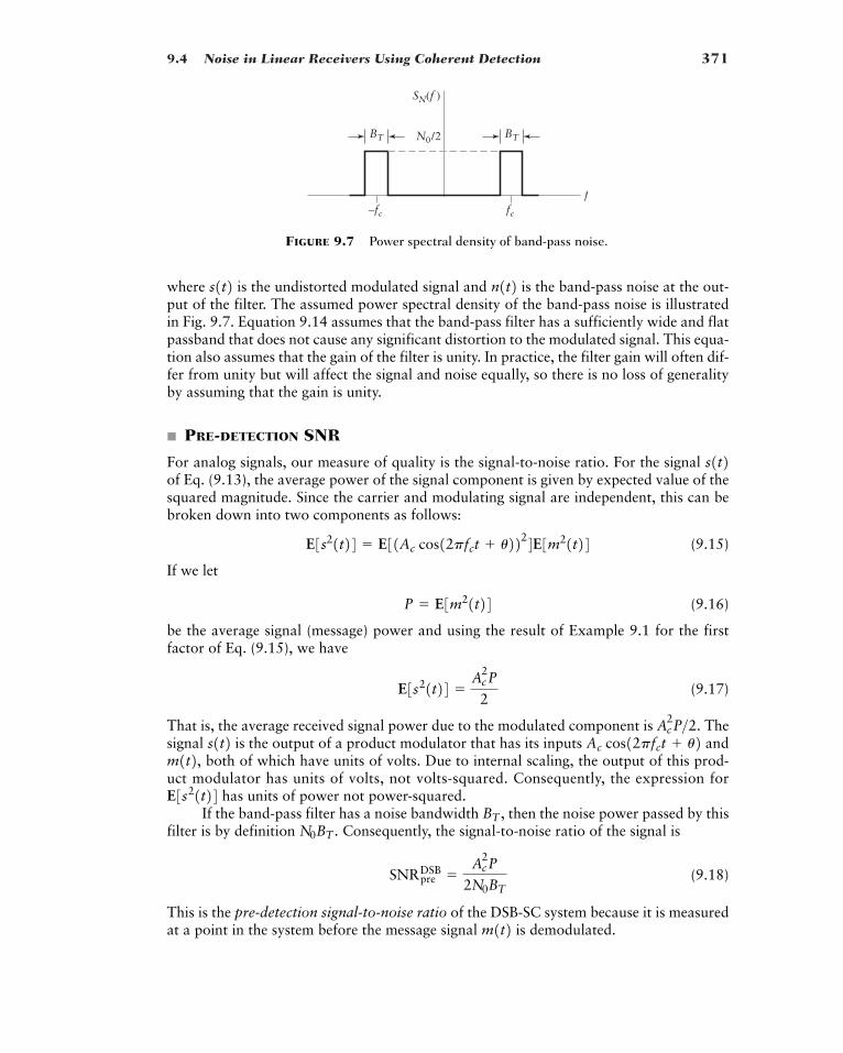
9.4 Noise in Linear Receivers Using Coherent Detection 371
f
SN(f )
BT BTN0/2
–fc fc
FIGURE 9.7 Power spectral density of band-pass noise.
where is the undistorted modulated signal and is the band-pass noise at the out-put of the filter. The assumed power spectral density of the band-pass noise is illustratedin Fig. 9.7. Equation 9.14 assumes that the band-pass filter has a sufficiently wide and flatpassband that does not cause any significant distortion to the modulated signal. This equa-tion also assumes that the gain of the filter is unity. In practice, the filter gain will often dif-fer from unity but will affect the signal and noise equally, so there is no loss of generalityby assuming that the gain is unity.
� PRE-DETECTION SNR
For analog signals, our measure of quality is the signal-to-noise ratio. For the signal of Eq. (9.13), the average power of the signal component is given by expected value of thesquared magnitude. Since the carrier and modulating signal are independent, this can bebroken down into two components as follows:
(9.15)
If we let
(9.16)
be the average signal (message) power and using the result of Example 9.1 for the firstfactor of Eq. (9.15), we have
(9.17)
That is, the average received signal power due to the modulated component is Thesignal is the output of a product modulator that has its inputs and
both of which have units of volts. Due to internal scaling, the output of this prod-uct modulator has units of volts, not volts-squared. Consequently, the expression for
has units of power not power-squared.If the band-pass filter has a noise bandwidth then the noise power passed by this
filter is by definition Consequently, the signal-to-noise ratio of the signal is
(9.18)
This is the pre-detection signal-to-noise ratio of the DSB-SC system because it is measuredat a point in the system before the message signal is demodulated.m1t2
SNRpreDSB �
Ac2P
2N0BT
N0BT .BT ,
E3s21t24m1t2, Ac cos12pfct u2s1t2 Ac
2P>2.
E3s21t24 �Ac
2P
2
P � E3m21t24
E3s21t24 � E31Ac cos12pfct u2224E3m21t24
s1t2
n1t2s1t2
372 CHAPTER 9 � NOISE IN ANALOG COMMUNICATIONS
� POST-DETECTION SNR
Next, we wish to determine the post-detection or output SNR of the DSB-SC system. Thepost-detection signal-to-noise ratio is the ratio of the message signal power to the noisepower after demodulation/detection. The post-detection SNR depends on both the modu-lation and demodulation techniques.
Using the narrowband representation of the band-pass noise, the signal at the inputto the coherent detector of Fig. 9.6 may be represented as
(9.19)
where and are the in-phase and quadrature components of with respectto the carrier. The output of mixer 2 in Fig. 9.6 is given by
(9.20)
where we have used the double-angle formulas
Note that the second line of Eq. (9.20) has two parts: the first part represents the basebandsignal and in-phase component of the noise, while the second part represents quadraturecomponent of its noise centered at the much higher frequency of These high-frequencycomponents are removed with a low-pass filter as shown in Fig. 9.6, and the result is
(9.21)
In Eqs. (9.20) and (9.21) we assume the gains of the second mixer and the low-pass filterare unity, without loss of generality. Two observations can be made:
� The message signal and the in-phase component of the filtered noise appearadditively in the output.
� The quadrature component of the noise is completely rejected by the demodulator.
From Eq. (9.21), we may compute the output or post-detection signal to noise ratio bynoting the following:
� The message component is so analogous to the computation of the pre-detection signal power, the post-detection signal power is where P is the aver-age message power as defined in Eq. (9.16).
� The noise component is after low-pass filtering. As described in Section 8.11, thein-phase component has a noise spectral density of over the bandwidth from to If the low-pass filter has a noise bandwidth W, corresponding to the messagebandwidth, which is less than or equal to then the output noise power is
(9.22)
Thus the power in is 2N0W.nI1t2� 2N0W
E3nI21t24 � L
W
�WN0 df
BT>2,BT>2.
�BT>2N0
12 nI1t2
14 Ac
2P
12 Acm1t2,
nI1t2m1t2
y1t2 � 12 1Acm1t2 nI1t22
2fc .
cos A cos A �1 cos 2A
2and sin A cos A �
sin 2A2
12 1Acm1t2 nI1t22 cos14pfct2 � 1
2 nQ1t2 sin14pfct2� 1
2 1Acm1t2 nI1t22v1t2 � x1t2 cos12pfct2
n1t2nQ1t2nI1t2x1t2 � s1t2 nI1t2 cos12pfct2 � nQ1t2 sin12pfct2
9.5 Noise In AM Receivers Using Envelope Detection 373
Combining these observations, we obtain the post-detection SNR of
(9.23)
Consequently, if the post-detection SNR is twice the pre-detection SNR. Thisis due to the fact that the quadrature component of the noise has been discarded by thesynchronous demodulator.
� FIGURE OF MERIT
It should be clear that for the reference transmission model defined in Section 9.2, the aver-age noise power for a message of bandwidth W is For DSB-SC modulation the aver-age modulated message power is given by Eq. (9.17), and consequently the reference SNRfor this transmission scheme is The corresponding figure of meritfor this receiver is
This illustrates that we lose nothing in performance by using a band-pass modulationscheme compared to the baseband modulation scheme, even though the bandwidth of theformer is twice as wide. Consequently, DSB-SC modulation provides a baseline againstwhich we may compare other amplitude modulation detection schemes.
� Drill Problem 9.2 A DSC-SC modulated signal is transmitted over a noisy channel, hav-ing a noise spectral density of watts per hertz. The message bandwidth is 4kHz and the carrier frequency is 200 kHz. Assume that the average received power of the sig-nal is Determine the post-detection signal-to-noise ratio of the receiver. �
9.5 Noise In AM Receivers Using Envelope Detection
In Section 3.1, we discussed envelope detection of amplitude modulation with a non-suppressed carrier. Envelope detection results in a simpler receiver than the coherentapproach as it does not require the circuitry to produce a synchronized carrier fordemodulation. Recall from Section 3.1 that the envelope-modulated signal is repre-sented by
(9.24)
where is the carrier wave, is the message signal, and is the amplitudesensitivity of the modulator. For envelope detection, the receiver model is depicted in Fig. 9.8. The front end of this receiver is identical to that of the coherent receiver. That is,the received signal, including additive noise, is passed through a band-pass filter.
kam1t2Ac cos12pfct2s1t2 � Ac11 kam1t22 cos12pfct2
�80 dBm.
2 10�17N0>2
Figure of merit �SNRpost
DSB
SNRref� 1
SNRref � Ac2P>(2N0W).
N0W.
W � BT>2,
�Ac
2P
2N0W
SNRpostDSB �
14 1Ac
22P14 12N0W2
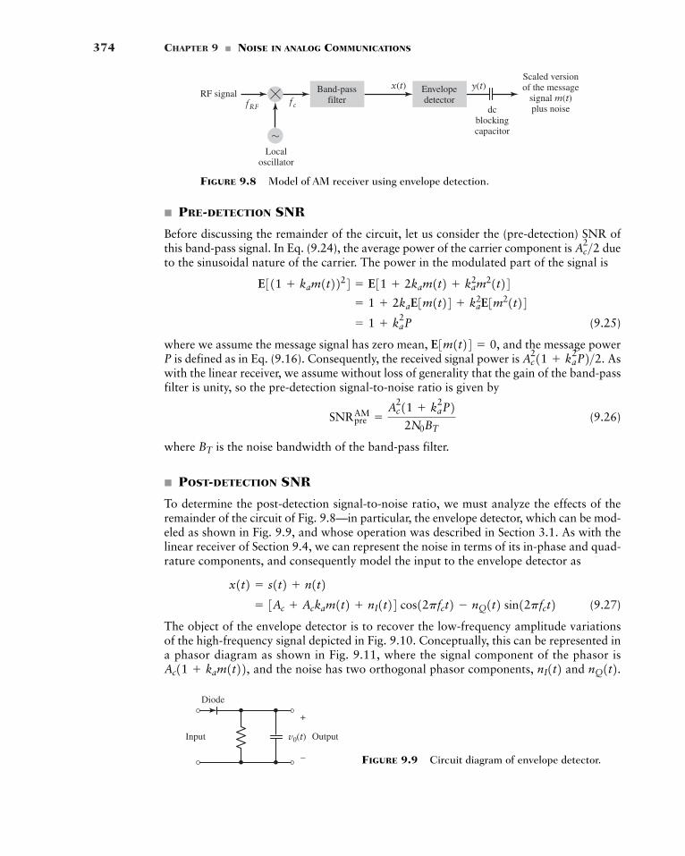
374 CHAPTER 9 � NOISE IN ANALOG COMMUNICATIONS
+
–
v0(t)Input Output
Diode
FIGURE 9.9 Circuit diagram of envelope detector.
Scaled versionof the message
signal m(t)plus noisedc
blockingcapacitor
Localoscillator
RF signalx(t) y(t)Envelope
detectorBand-pass
filterfRFfc
~
FIGURE 9.8 Model of AM receiver using envelope detection.
� PRE-DETECTION SNR
Before discussing the remainder of the circuit, let us consider the (pre-detection) SNR ofthis band-pass signal. In Eq. (9.24), the average power of the carrier component is dueto the sinusoidal nature of the carrier. The power in the modulated part of the signal is
(9.25)
where we assume the message signal has zero mean, and the message powerP is defined as in Eq. (9.16). Consequently, the received signal power is Aswith the linear receiver, we assume without loss of generality that the gain of the band-passfilter is unity, so the pre-detection signal-to-noise ratio is given by
(9.26)
where is the noise bandwidth of the band-pass filter.
� POST-DETECTION SNR
To determine the post-detection signal-to-noise ratio, we must analyze the effects of theremainder of the circuit of Fig. 9.8—in particular, the envelope detector, which can be mod-eled as shown in Fig. 9.9, and whose operation was described in Section 3.1. As with thelinear receiver of Section 9.4, we can represent the noise in terms of its in-phase and quad-rature components, and consequently model the input to the envelope detector as
(9.27)
The object of the envelope detector is to recover the low-frequency amplitude variationsof the high-frequency signal depicted in Fig. 9.10. Conceptually, this can be represented ina phasor diagram as shown in Fig. 9.11, where the signal component of the phasor is
and the noise has two orthogonal phasor components, and nQ1t2.nI1t2Ac11 kam1t22,
� 3Ac Ackam1t2 nI1t24 cos12pfct2 � nQ1t2 sin12pfct2x1t2 � s1t2 n1t2
BT
SNRpreAM �
Ac211 ka
2P22N0BT
Ac211 ka
2P2>2.E3m1t24 � 0,
� 1 ka2P
� 1 2kaE3m1t24 k2aE3m21t24
E311 kam1t2224 � E31 2kam1t2 k2am21t24
Ac2>2
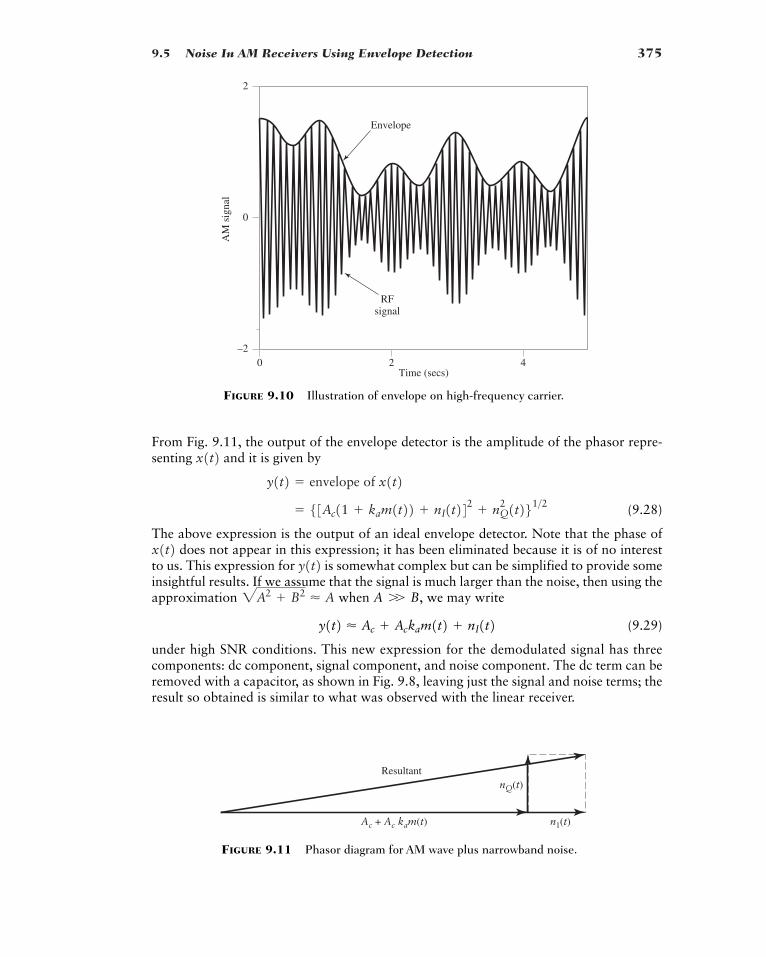
9.5 Noise In AM Receivers Using Envelope Detection 375
AM
sig
nal
Time (secs)
Envelope
RFsignal
0 2 4–2
0
2
FIGURE 9.10 Illustration of envelope on high-frequency carrier.
n1(t)Ac + Ac kam(t)
nQ(t)Resultant
FIGURE 9.11 Phasor diagram for AM wave plus narrowband noise.
From Fig. 9.11, the output of the envelope detector is the amplitude of the phasor repre-senting and it is given by
(9.28)
The above expression is the output of an ideal envelope detector. Note that the phase ofdoes not appear in this expression; it has been eliminated because it is of no interest
to us. This expression for is somewhat complex but can be simplified to provide someinsightful results. If we assume that the signal is much larger than the noise, then using theapproximation when we may write
(9.29)
under high SNR conditions. This new expression for the demodulated signal has threecomponents: dc component, signal component, and noise component. The dc term can beremoved with a capacitor, as shown in Fig. 9.8, leaving just the signal and noise terms; theresult so obtained is similar to what was observed with the linear receiver.
y1t2 � Ac Ackam1t2 nI1t2A W B,2A2 B2 � A
y1t2x1t2� 53Ac11 kam1t22 nI1t242 nQ
2 1t261>2y1t2 � envelope of x1t2
x1t2
376 CHAPTER 9 � NOISE IN ANALOG COMMUNICATIONS
2See Chapter 2 of Haykin (2001).
Accordingly, the post-detection SNR for the envelope detection of AM, using a mes-sage bandwidth W, is given by
(9.30)
where the numerator represents the average power of the message and the denom-inator represents the average power of from Eq. (9.22).
This evaluation of the output SNR is only valid under two conditions:
� The SNR is high.� is adjusted for 100% modulation or less, so there is no distortion of the signal
envelope.
As with suppressed-carrier amplitude modulation, the message bandwidth W is approxi-mately one-half of the transmission bandwidth
� FIGURE OF MERIT
For AM modulation, the average transmitted power is given by the product of Eq. (9.25)and the carrier power consequently the reference SNR is Com-bining this result with Eq. (9.30), the figure of merit for this AM modulation–demodulation scheme is
(9.31)
Since the product is always less than unity (otherwise the signal would be over mod-ulated), the figure of merit for this system is always less than 0.5. Hence, the noise perfor-mance of an envelope-detector receiver is always inferior to a DSB-SC receiver, the reasonis that at least half of the power is wasted transmitting the carrier as a component of themodulated (transmitted) signal.
This completes the noise analysis of envelope modulation, but we note that a math-ematical analysis can also be performed when the signal-to-noise ratio is low.2 From Eq.(9.30), we see that the post-detection SNR has an inverse linear dependence on the noisespectral density. With low signal-to-noise conditions, nonlinear effects appear. Synchro-nous detection does not have this nonlinear behavior, but the quality of the voice is still poorat low post-detection SNRs.
� COMPUTER EXPERIMENT: ENVELOPE DETECTION
In Problem 9.26, we describe a computer experiment that simulates envelope detectionusing the phasor notation given above. In the experiment, the message is a sinusoidal wave
for which we create a time-varying phasor and add a correspond-ing noise phasor. In this experiment, we compute the pre-detection and post-detectionSNRs for samples of its signal. These two measures are plotted against one another in Fig.9.12 for . Also shown in this plot is the theoretical performance of these two mea-sures as given by Eqs. (9.26) and (9.30).
ka � 0.3
m1t2 � A sin12pfmt2,
ka2P
Figure of merit �SNRpost
AM
SNRref�
ka2P
1 ka2P
Ac211 ka
2P2>(2N0W ).Ac2>2;
BT .
ka
nI1t2 Ackam1t2,SNRpost
AM �Ac
2ka2P
2N0W
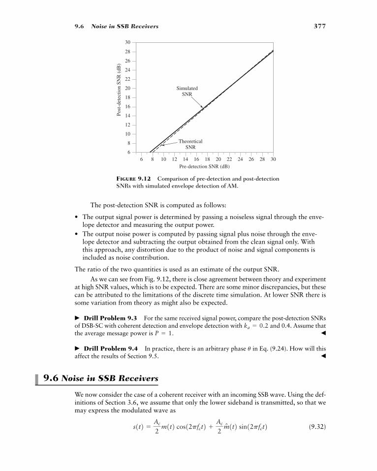
9.6 Noise in SSB Receivers 377
The post-detection SNR is computed as follows:
• The output signal power is determined by passing a noiseless signal through the enve-lope detector and measuring the output power.
• The output noise power is computed by passing signal plus noise through the enve-lope detector and subtracting the output obtained from the clean signal only. Withthis approach, any distortion due to the product of noise and signal components isincluded as noise contribution.
The ratio of the two quantities is used as an estimate of the output SNR.
As we can see from Fig. 9.12, there is close agreement between theory and experimentat high SNR values, which is to be expected. There are some minor discrepancies, but thesecan be attributed to the limitations of the discrete time simulation. At lower SNR there issome variation from theory as might also be expected.
� Drill Problem 9.3 For the same received signal power, compare the post-detection SNRsof DSB-SC with coherent detection and envelope detection with and 0.4. Assume thatthe average message power is �
� Drill Problem 9.4 In practice, there is an arbitrary phase in Eq. (9.24). How will thisaffect the results of Section 9.5. �
9.6 Noise in SSB Receivers
We now consider the case of a coherent receiver with an incoming SSB wave. Using the def-initions of Section 3.6, we assume that only the lower sideband is transmitted, so that wemay express the modulated wave as
(9.32)s1t2 �Ac
2m1t2 cos12pfct2
Ac
2mN 1t2 sin12pfct2
u
P � 1.ka � 0.2
SimulatedSNR
TheoreticalSNR
6 8 10 12 14 16 18Pre-detection SNR (dB)
Post
-det
ectio
n SN
R (
dB)
20 22 24 26 28 306
8
10
12
14
16
18
20
22
24
26
28
30
FIGURE 9.12 Comparison of pre-detection and post-detectionSNRs with simulated envelope detection of AM.
378 CHAPTER 9 � NOISE IN ANALOG COMMUNICATIONS
where is the Hilbert transform of the message signal We may make the fol-lowing observations concerning the in-phase and quadrature components of in Eq. (9.32):
1. The two components and are uncorrelated with each other. Therefore,their power spectral densities are additive.
2. The Hilbert transform is obtained by passing through a linear filter withtransfer function The squared magnitude of this transfer function is equalto one for all Accordingly, and have the same average power P.
Thus, proceeding in a manner similar to that for the DSB-SC receiver, we find that the in-phaseand quadrature components of the SSB modulated wave contribute an average power of
each. The average power of is therefore This result is half that of the DSB-SC case, which is intuitively satisfying.
� PRE-DETECTION SNR
For the SSB signal, the transmission bandwidth is approximately equal to the messagebandwidth W. Consequently, using the signal power calculation of the previous section, thepre-detection signal-to-noise ratio of a coherent receiver with SSB modulation is
(9.33)
� POST-DETECTION SNR
Using the same superheterodyne receiver of Figure 9.6, the band-pass signal after multi-plication with the synchronous oscillator output is
(9.34)
After low-pass filtering the we are left with
(9.35)
As expected, we see that the quadrature component of the message signal has beeneliminated from the detector output. With a band-pass filter tailor-made for the SSB sig-nal, the band-pass noise will also be of single sideband nature. However, as noted inEq. (8.98), the spectrum of the in-phase component of the noise is given by
(9.36)SNI1f2 � bSN1f � fc2 SN1f fc2, �B � f � B
0, otherwise
nI1t2n1t2mN 1t2
y1t2 � 12 ¢Ac
2m1t2 nI1t2≤v1t2,
12 ¢Ac
2m1t2 nI1t2≤ cos14pfct2 � 1
2 ¢Ac
2mN 1t2 nQ1t2≤ sin14pfct2
� 12 ¢Ac
2m1t2 nI1t2≤v1t2 � x1t2 cos12pfct2
cos12pfct2
SNRSSBpre �
Ac2P
4N0W
BT
Ac2P>4.s1t2Ac
2P>8 s1t2mN 1t2m1t2f.
�j sgn1f2. m1t2mN 1t2mN 1t2m1t2
s1t2m1t2.mN 1t2
9.6 Noise in SSB Receivers 379
For the single sideband case, is for and forConsequently,
(9.37)
In other words, the spectral density of is double-sided, as in the DSB-SC case, but withhalf of the power. In a practical application, the SSB filter will attenuate the low-frequencycomponents of the signal plus noise. Hence, in practice, the spectrum of will often havea notch at dc.
From Eq. (9.35), the message component in the receiver output is so thatthe average power of the recovered message is The corresponding noise power fromEqs. (9.35) and (9.37) is Accordingly, the post-detection signal-to-noise ratio of asystem using SSB modulation in the transmitter and coherent detection in the receiver is theratio of these two powers; namely,
(9.38)
� FIGURE OF MERIT
The average signal power for the SSB system, as discussed above, is Consequently,the reference SNR is The figure of merit for the SSB system is the ratio ofEq. (9.38) to the latter; that is,
(9.39)
Consequently, SSB transmission has the same figure of merit as DSB-SC. The performanceof vestigial sideband with coherent detection is similar to that of SSB.
Comparing the results for the different amplitude modulation schemes, we find thatthere are a number of design tradeoffs. Double-sideband suppressed carrier modulationprovides the same SNR performance as the baseband reference model but requires syn-chronization circuitry to perform coherent detection. Non-suppressed-carrier AM simpli-fies the receiver design significantly as it is implemented with an envelope detector. However,non-suppressed-carrier AM requires significantly more transmitter power to obtain thesame SNR performance as the baseband reference model. Single-sideband modulationachieves the same SNR performance as the baseband reference model but only requireshalf the transmission bandwidth of the DSC-SC system. On the other hand, SSB requiresmore transmitter processing. These observations are our first indication that communica-tion system design involves a tradeoff between power, bandwidth, and processingcomplexity.
� Drill Problem 9.5 The message signal of Problem 9.2 having a bandwidth W of 4 kHzis transmitted over the same noisy channel having a noise spectral density of watts per hertz using single-sideband modulation. If the average received power of the signal is
what is the post-detection signal-to-noise ratio of the receiver? Compare the trans-mission bandwidth of the SSB receiver to that of the DSB-SC receiver. �
�80 dBm,
2 10�17N0>2
Figure of merit �SNRpost
SSB
SNRref� 1
Ac2P>14N0W2. Ac
2P>4.
SNRSSBpost �
Ac2P
4NoW
14 N0W.
Ac2P>16.
Acm1t2>4nI1t2
nI1t2SNI1f2 � c N0
2, �W � f � W
0, otherwise
�fc � W � f � �fc .fc � f � fc WN0>2SN1f2
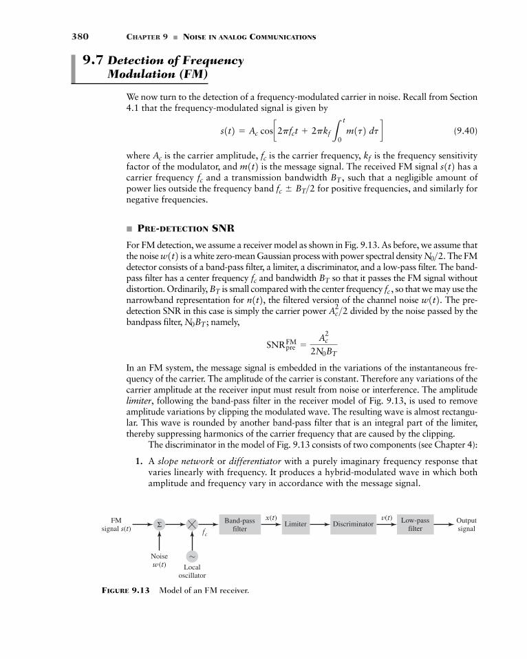
380 CHAPTER 9 � NOISE IN ANALOG COMMUNICATIONS
9.7 Detection of Frequency Modulation (FM)
We now turn to the detection of a frequency-modulated carrier in noise. Recall from Section4.1 that the frequency-modulated signal is given by
(9.40)
where is the carrier amplitude, is the carrier frequency, is the frequency sensitivityfactor of the modulator, and is the message signal. The received FM signal has acarrier frequency and a transmission bandwidth such that a negligible amount ofpower lies outside the frequency band for positive frequencies, and similarly fornegative frequencies.
� PRE-DETECTION SNR
For FM detection, we assume a receiver model as shown in Fig. 9.13. As before, we assume thatthe noise is a white zero-mean Gaussian process with power spectral density The FMdetector consists of a band-pass filter, a limiter, a discriminator, and a low-pass filter. The band-pass filter has a center frequency and bandwidth so that it passes the FM signal withoutdistortion. Ordinarily, is small compared with the center frequency so that we may use thenarrowband representation for the filtered version of the channel noise The pre-detection SNR in this case is simply the carrier power divided by the noise passed by thebandpass filter, namely,
In an FM system, the message signal is embedded in the variations of the instantaneous fre-quency of the carrier. The amplitude of the carrier is constant. Therefore any variations of thecarrier amplitude at the receiver input must result from noise or interference. The amplitudelimiter, following the band-pass filter in the receiver model of Fig. 9.13, is used to removeamplitude variations by clipping the modulated wave. The resulting wave is almost rectangu-lar. This wave is rounded by another band-pass filter that is an integral part of the limiter,thereby suppressing harmonics of the carrier frequency that are caused by the clipping.
The discriminator in the model of Fig. 9.13 consists of two components (see Chapter 4):
1. A slope network or differentiator with a purely imaginary frequency response thatvaries linearly with frequency. It produces a hybrid-modulated wave in which bothamplitude and frequency vary in accordance with the message signal.
SNRpreFM �
Ac2
2N0BT
N0BT ;Ac
2>2 w1t2.n1t2, fc ,BT
BTfc
N0>2.w1t2
fc � BT>2 BT ,fcs1t2m1t2 kffcAc
s1t2 � Ac cos c2pfct 2pkfLt
0m1t2 dt d
Band-passfilter
Limiter DiscriminatorΣ Low-passfilter
Noisew(t) Local
oscillator
v(t)x(t)FMsignal s(t)
Outputsignalfc
~
FIGURE 9.13 Model of an FM receiver.
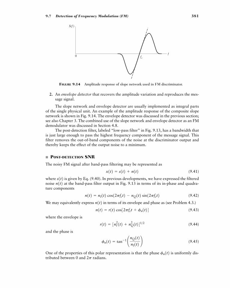
9.7 Detection of Frequency Modulation (FM) 381
ffc
S(f )
0
2. An envelope detector that recovers the amplitude variation and reproduces the mes-sage signal.
The slope network and envelope detector are usually implemented as integral partsof the single physical unit. An example of the amplitude response of the composite slopenetwork is shown in Fig. 9.14. The envelope detector was discussed in the previous section;see also Chapter 3. The combined use of the slope network and envelope detector as an FMdemodulator was discussed in Section 4.8.
The post-detection filter, labeled “low-pass filter” in Fig. 9.13, has a bandwidth thatis just large enough to pass the highest frequency component of the message signal. Thisfilter removes the out-of-band components of the noise at the discriminator output andthereby keeps the effect of the output noise to a minimum.
� POST-DETECTION SNR
The noisy FM signal after band-pass filtering may be represented as
(9.41)
where is given by Eq. (9.40). In previous developments, we have expressed the filterednoise at the band-pass filter output in Fig. 9.13 in terms of its in-phase and quadra-ture components
(9.42)
We may equivalently express in terms of its envelope and phase as (see Problem 4.3.)
(9.43)
where the envelope is
(9.44)
and the phase is
(9.45)
One of the properties of this polar representation is that the phase is uniformly dis-tributed between 0 and radians.2p
fn1t2fn1t2 � tan�1 ¢nQ1t2
nI1t2 ≤r1t2 � 3nI
21t2 nQ2 1t241>2
n1t2 � r1t2 cos32pfct fn1t24n1t2
n1t2 � nI1t2 cos12pfct2 � nQ1t2 sin12pfct2n1t2s1t2
x1t2 � s1t2 n1t2
FIGURE 9.14 Amplitude response of slope network used in FM discriminator.
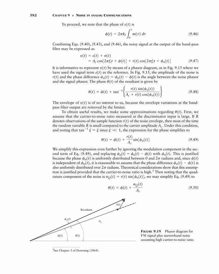
382 CHAPTER 9 � NOISE IN ANALOG COMMUNICATIONS
Ac
Resultant
r(t)
�n(t)
�(t) �(t)FIGURE 9.15 Phasor diagram forFM signal plus narrowband noiseassuming high carrier-to-noise ratio.
3See Chapter 5 of Downing (1964).
To proceed, we note that the phase of is
(9.46)
Combining Eqs. (9.40), (9.43), and (9.46), the noisy signal at the output of the band-passfilter may be expressed as
(9.47)
It is informative to represent by means of a phasor diagram, as in Fig. 9.15 where wehave used the signal term as the reference. In Fig. 9.15, the amplitude of the noise is
and the phase difference is the angle between the noise phasorand the signal phasor. The phase of the resultant is given by
(9.48)
The envelope of is of no interest to us, because the envelope variations at the band-pass filter output are removed by the limiter.
To obtain useful results, we make some approximations regarding First, weassume that the carrier-to-noise ratio measured at the discriminator input is large. If Rdenotes observations of the sample function of the noise envelope, then most of the timethe random variable R is small compared to the carrier amplitude Under this condition,and noting that since the expression for the phase simplifies to
(9.49)
We simplify this expression even further by ignoring the modulation component in the sec-ond term of Eq. (9.49), and replacing with This is justifiedbecause the phase is uniformly distributed between 0 and radians and, since is independent of it is reasonable to assume that the phase difference isalso uniformly distributed over radians. Theoretical considerations show that this assump-tion is justified provided that the carrier-to-noise ratio is high.3 Then noting that the quad-rature component of the noise is we may simplify Eq. (9.49) to
(9.50)u1t2 � f1t2 nQ1t2
Ac
nQ1t2 � r1t2 sin3fn1t24,2p
fn1t2 � f1t2fn1t2, f1t22pfn1t2 fn1t2.cn1t2 � fn1t2 � f1t2u1t2 � f1t2
r1t2Ac
sin3cn1t24j V 1,tan�1 j � j
Ac .r1t2
u1t2.x1t2
u1t2 � f1t2 tan�1b r1t2 sin1cn1t22Ac r1t2 cos1cn1t22 r
u1t2cn1t2 � fn1t2 � f1t2r1t2 s1t2x1t2� Ac cos32pfct f1t24 r1t2 cos32pfct fn1t24
x1t2 � s1t2 n1t2
f1t2 � 2pkfLt
0m1t2 dt
s1t2
9.7 Detection of Frequency Modulation (FM) 383
Using the expression for given by Eq. (9.46), Eq. (9.50) can be expressed as
(9.51)
Our objective is to determine the error in the instantaneous frequency of the carrier wavecaused by the presence of the filtered noise With an ideal discriminator, its output isproportional to the derivative Using the expression for in Eq. (9.51), theideal discriminator output, scaled by is therefore
(9.52)
where the noise term is defined by
(9.53)
We now see that, provided the carrier-to-noise ratio is high, the discriminator output consists of the original message signal multiplied by the constant factor plus anadditive noise component The additive noise at the discriminator output is determinedessentially by the quadrature component of the narrowband noise .
Accordingly, we may use the post-detection signal-to-noise ratio, as previously defined,to assess the output quality of the FM receiver. The post-detection signal-to-noise ratio isdefined as the ratio of the average output signal power to the average output noise power.From Eq. (9.52) we see that the message component of the discriminator output, and there-fore the low-pass filter output, is Hence, the average output signal power is equalto where P is the average power of the message signal
To determine the average output noise power, we note that the noise at the dis-criminator output is proportional to the time derivative of the quadrature noise component
Since the differentiation of a function with respect to time corresponds to multipli-cation of its Fourier transform by it follows that we may obtain the noise process by passing through a linear filter with a frequency response equal to
(9.54)
This means that the power spectral density of the noise is related to the powerspectral density of the quadrature noise component as follows:
(9.55)
With the band-pass filter in the receiver model of Fig. 9.13 having an ideal frequencyresponse characterized by bandwidth and midband frequency it follows that the nar-rowband noise will have a power spectral density characteristic that is similarly shaped.If the input noise is white then, from the properties of the in-phase and quadrature com-ponents of narrowband noise described in Section 8.11, the power spectral density of will be the low-pass equivalent of the sum of the positive and negative frequency responsesof the band-pass filter. This means that the quadrature component of the narrowbandnQ1t2
nQ1t2n1t2 fc ,BT
�f 2
Ac2 SNQ
1f2SNd1f2 � ƒG1f2 ƒ2SNQ
1f2nQ1t2SNQ
1f2 nd1t2SNd1f2
G1f2 �j2pf
2pAc�
jf
Ac
nQ1t2 nd1t2j2pf,nQ1t2.
nd1t2m1t2.kf2P
kf m1t2.
n1t2nQ1t2nd1t2. kf ,m1t2 v1t2nd1t2 �
12pAc
dnQ1t2dt
nd1t2� kf m1t2 nd1t2
v1t2 �1
2pdu(t)
dt
2p,u1t2du1t2>dt.
n1t2.u1t2 � 2pkfL
t
0m1t2 dt
nQ1t2Ac
f1t2
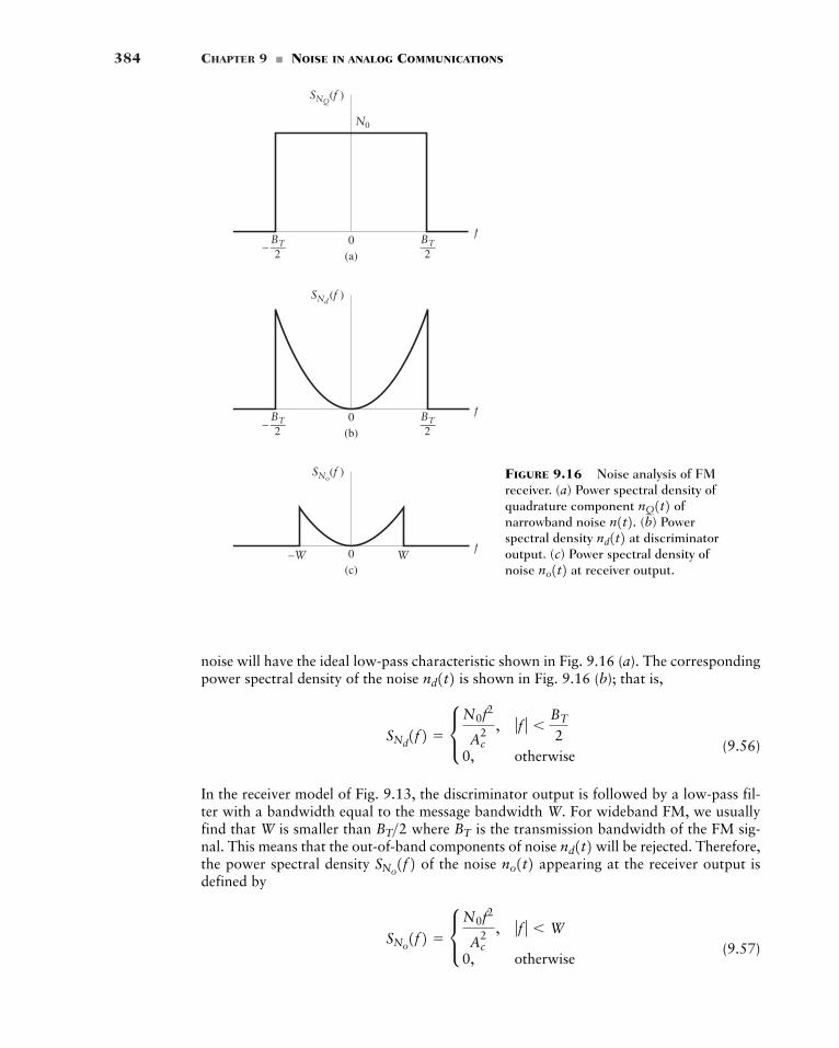
384 CHAPTER 9 � NOISE IN ANALOG COMMUNICATIONS
(a)
f
SNQ(f )
N0
0– —
BT2
—BT2
– —BT2
—BT2
f
(b)
SNd(f )
0
f
(c)
SNo(f )
0–W W
FIGURE 9.16 Noise analysis of FMreceiver. (a) Power spectral density ofquadrature component ofnarrowband noise (b) Powerspectral density at discriminatoroutput. (c) Power spectral density ofnoise at receiver output.no1t2
nd1t2n1t2.nQ1t2
noise will have the ideal low-pass characteristic shown in Fig. 9.16 (a). The correspondingpower spectral density of the noise is shown in Fig. 9.16 (b); that is,
(9.56)
In the receiver model of Fig. 9.13, the discriminator output is followed by a low-pass fil-ter with a bandwidth equal to the message bandwidth W. For wideband FM, we usuallyfind that W is smaller than where is the transmission bandwidth of the FM sig-nal. This means that the out-of-band components of noise will be rejected. Therefore,the power spectral density of the noise appearing at the receiver output isdefined by
(9.57)SNo1f2 � c N0f2
Ac2 , ƒf ƒ � W
0, otherwise
no1t2SNo1f2 nd1t2BTBT>2
SNd1f2 � c N0f2
Ac2 , ƒf ƒ �
BT
20, otherwise
nd1t2
9.7 Detection of Frequency Modulation (FM) 385
as shown in Fig. 9.16(c). The average output noise power is determined by integrating thepower spectral density from to W. Doing so, we obtain the following result:
(9.58)
From Eqs. (9.52) and (9.16) the average output signal power is As mentioned earlier,provided the carrier-to-noise ratio is high, the post-detection signal-to-noise ratio is equalto the ratio of to the right-hand side of Eq. (9.58), thereby yelding
(9.59)
Hence, the post-detection SNR of an FM demodulator has a nonlinear dependence on boththe frequency sensitivity and the message bandwidth.
� FIGURE OF MERIT
With FM modulation, the modulated signal power is simply hence the reference SNRis Consequently, the figure of merit for this system is given by
(9.60)
where, in the last line, we have introduced the definition as the deviationratio for the FM system in light of the material presented in Section 4.6. Recall from thatsection that the generalized Carson rule yields the transmission bandwidth
for an FM signal. So, substituting for in thedefinition of D, the figure of merit for an FM system is approximately given by
(9.61)
Consequently, an increase in the transmission bandwidth provides a correspondingquadratic increase in the output signal-to-noise ratio with an FM system compared to thereference system. Thus, when the carrier to noise level is high, unlike an amplitude modu-lation system an FM system allows us to trade bandwidth for improved performance inaccordance with a square law.
EXAMPLE 9.2 Noise in FM Multiplexed Channels
In the FM stereo multiplexing strategy described in Section 4.9, we wish to determine the post-detection SNR of the stereo difference signal assuming that the transmissionbandwidth is 200 kHz, the baseband bandwidth is 19 kHz, and the pre-detection SNR is 12 dB.
ml1t2 � mr1t2,
BT
Figure of merit �34¢BT
W≤2
kfP1>2BT>2BT � 21kfP
1>2 W2 � 2kfP1>2
D � kfP1>2>W
� 3D2
� 3¢kf2P
W2 ≤Figure of merit �
SNRpostFM
SNRref�
3Ac2kf
2P
2N0W3
Ac2
2N0W
Ac2>(2N0W ).
Ac2>2,
SNRpostFM �
3Ac2kf
2P
2N0W3
kf2P
kf2P.
�2N0W3
3Ac2
Average post-detection noise power �N0
Ac2 L
W
�Wf 2 df
�WSNo1f2
386 CHAPTER 9 � NOISE IN ANALOG COMMUNICATIONS
From the material presented previously in this section, the pre-detection SNR is
Ignoring the pilot component, the average post-detection noise power in the upper channel ofthe FM multiplex is
The post-detection SNR on the upper channel is
where we have used the approximation to Carson’s rule that and have assumedthat half of the power is in the upper channel.
� THRESHOLD EFFECT
The formula of Eq. (9.59), defining the post-detection SNR ratio of an FM receiver, is validonly if the pre-detection SNR, measured at the discriminator input, is high compared tounity. If the pre-detection SNR is lowered, the FM receiver breaks down. At first, individ-ual clicks are heard in the receiver output, and as the pre-detection SNR decreases further,the clicks merge to a crackling or sputtering sound. At and below this breakdown point,Eq. (9.59) fails to accurately predict the post-detection SNR. This phenomenon is knownas the threshold effect; its evaluation is however beyond the scope of this book.
� COMPUTER EXPERIMENT: THRESHOLD EFFECT WITH FM
In Problem 9.27, we describe a computer experiment for simulating the detection of anFM signal in noise. The signal and noise are both generated using complex phasor nota-tion, but they are subsequently up-converted to an IF, creating a band-pass signal, to applydiscriminator detection.
The complex phasor of the FM signal is given by
where (for the results that follow) we have and hertz per unitamplitude. This signal was transmitted with a band-pass transmission bandwidth of
and a baseband detection bandwidth of W � 5.5 Hz.BT � 62.5 Hz
kf � 20m1t2 � sin12pt2s1t2 � Ac expe�j2pkfL
t
0m1t2 dt f
BT � 2kfP1>2
� 24.3 dB� 266.6
�Ac
2
2N0BT
3>452¢BT
W≤3
�Ac
2
2N0BT
352
kf2PBT
W3
SNRpost �3Ac
2kf21P>22
52N0W3
�52W3N0
3A2c
N �N0
Ac2 2L
3W
Wf 2 df
SNRpre �Ac
2
2N0BT
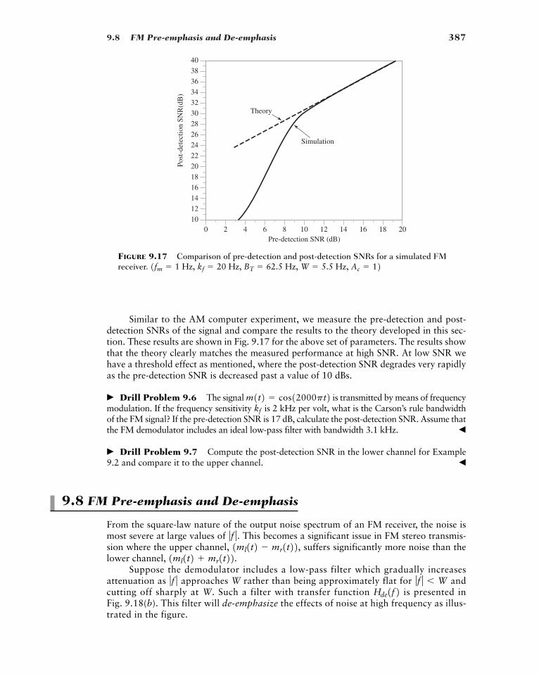
9.8 FM Pre-emphasis and De-emphasis 387
Similar to the AM computer experiment, we measure the pre-detection and post-detection SNRs of the signal and compare the results to the theory developed in this sec-tion. These results are shown in Fig. 9.17 for the above set of parameters. The results showthat the theory clearly matches the measured performance at high SNR. At low SNR wehave a threshold effect as mentioned, where the post-detection SNR degrades very rapidlyas the pre-detection SNR is decreased past a value of 10 dBs.
� Drill Problem 9.6 The signal is transmitted by means of frequencymodulation. If the frequency sensitivity is 2 kHz per volt, what is the Carson’s rule bandwidthof the FM signal? If the pre-detection SNR is 17 dB, calculate the post-detection SNR. Assume thatthe FM demodulator includes an ideal low-pass filter with bandwidth 3.1 kHz. �
� Drill Problem 9.7 Compute the post-detection SNR in the lower channel for Example9.2 and compare it to the upper channel. �
9.8 FM Pre-emphasis and De-emphasis
From the square-law nature of the output noise spectrum of an FM receiver, the noise ismost severe at large values of This becomes a significant issue in FM stereo transmis-sion where the upper channel, suffers significantly more noise than thelower channel,
Suppose the demodulator includes a low-pass filter which gradually increasesattenuation as approaches W rather than being approximately flat for andcutting off sharply at W. Such a filter with transfer function is presented inFig. 9.18(b). This filter will de-emphasize the effects of noise at high frequency as illus-trated in the figure.
Hde1f2 ƒf ƒ � Wƒf ƒ
1ml1t2 mr1t22.1ml1t2 � mr1t22,ƒf ƒ .
kf
m1t2 � cos12000pt2
Post
-det
ectio
n SN
R(d
B)
0 2 4 6 8 10 12 14 16 18 2010
12
14
16
18
20
22
24
26
28
30
32
34
36
38
40
Pre-detection SNR (dB)
Simulation
Theory
FIGURE 9.17 Comparison of pre-detection and post-detection SNRs for a simulated FMreceiver. 1fm � 1 Hz, kf � 20 Hz, BT � 62.5 Hz, W � 5.5 Hz, Ac � 12
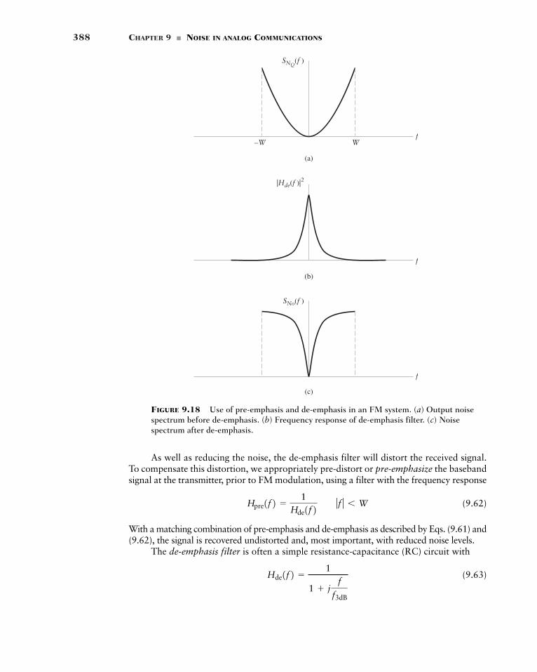
388 CHAPTER 9 � NOISE IN ANALOG COMMUNICATIONS
(b)
|Hde(f )|2
f
(c)
SNo(f )
f
(a)
f–W W
SNQ(f )
FIGURE 9.18 Use of pre-emphasis and de-emphasis in an FM system. (a) Output noisespectrum before de-emphasis. (b) Frequency response of de-emphasis filter. (c) Noisespectrum after de-emphasis.
As well as reducing the noise, the de-emphasis filter will distort the received signal.To compensate this distortion, we appropriately pre-distort or pre-emphasize the basebandsignal at the transmitter, prior to FM modulation, using a filter with the frequency response
(9.62)
With a matching combination of pre-emphasis and de-emphasis as described by Eqs. (9.61) and(9.62), the signal is recovered undistorted and, most important, with reduced noise levels.
The de-emphasis filter is often a simple resistance-capacitance (RC) circuit with
(9.63)Hde1f2 �1
1 jf
f3dB
Hpre1f2 �1
Hde1f2 ƒf ƒ � W
9.8 FM Pre-emphasis and De-emphasis 389
This filter is approximately flat for the 3-dB bandwidth of the filter. With thischoice, the noise spectrum for becomes flat over most of the message bandwidthas shown in Figure 9.18(c).
At the transmitting end, the pre-emphasis filter is
(9.64)
This second filter has little effect at low frequencies where At frequencies(recall that the transfer function of a differentiator is ), the filter of Eq. (9.64)
is approximately equivalent to a differentiator. Thus the pre-emphasized signal is the sumof the original signal plus its derivative. Consequently, the modulated signal is approximately
where Thus, pre-emphasized FM is really a combination of frequency modu-lation and phase modulation.
Pre-emphasis is used in many applications other than FM stereo broadcasting. Pre-emphasis can be used to advantage whenever portions of the message band are degradedrelative to others. That is, portions of the message band that are most sensitive to noise areamplified (emphasized) before transmission. At the receiver, the signal is de-emphasized toreverse the distortion introduced by the transmitter; at the same time the de-emphasisreduces the noise that falls in the most sensitive part of the message band. For example, theDolby system for tape recording pre-emphasizes high frequencies for sound recording sothat high-frequency surface noise can be de-emphasized during playback.
EXAMPLE 9.3 Pre-emphasis Improvement
In this example, we address the improvement in the post-detection signal-to-noise ratio of anFM receiver with the pre-and de-emphasis networks of Eqs. (9.64) and (9.63).
From Eq. (9.58), the noise power without de-emphasis is given by
The corresponding noise power with de-emphasis is given by
The improvement provided by de-emphasis is the ratio of these last two expressions,
I �N
Nde�
1W>f3dB23331W>f3dB2 � tan�11W>f3dB24
� 2N0
Ac2 31W>f3dB2 � tan�11W>f3dB241f3dB23
Nde � LW
�W
N0f 2>Ac2
1 1f>f3dB22 df
N �23
N0W3
Ac2
a � 1>f3dB.
� Ac cosa2pfct 2pkfLt
0m1s2 ds 2pkfam1t2b
s1t2 � Ac cosa2pfct 2pkfLt
0am1s2 a
dm1s2dsb dsb
j2pfƒf ƒ � f3dB
ƒf ƒ � f3dB.
Hpre1f2 � 1 jf
f3dB
ƒf ƒ � f3dB
ƒf ƒ � f3dB,
390 CHAPTER 9 � NOISE IN ANALOG COMMUNICATIONS
In commercial FM broadcasting, we typically have and we may reasonablyassume This set of values yields which corresponds to an improvementof 13 dB in the post-detection signal-to-noise ratio of the receiver. This example illustrates thata significant improvement in the noise performance of an FM system may be achieved by usingpre-emphasis and de-emphasis filters made up of simple RC circuits.
� Drill Problem 9.8 An FM system has a pre-detection SNR of 15 dB. If the trans-mission bandwidth is 30 MHz and the message bandwidth is 6 MHz, what is the post-detec-tion SNR? Suppose the system includes pre-emphasis and de-emphasis filters as described byEqs. (9.63) and (9.64). What is the post-detection SNR if the of the de-emphasis filteris 800 kHz? �
9.9 Summary and Discussion
In this chapter, we looked at the detection of various analog modulated signals in the pres-ence of additive noise. We began by reviewing the characteristics of Gaussian noise, the mostcommon impairment in communication systems. We next introduced the concepts of pre-detection and post-detection signal-to-noise ratio (SNR) and established the ratio of thepost-detection SNR to the SNR of a baseband reference model as the figure of merit for com-paring analog communication systems.
Subsequently, we analyzed the noise performance of a number of different amplitudemodulation schemes and found:
(i) The detection of DSB-SC with a linear coherent receiver has the same SNR perfor-mance as the baseband reference model but requires synchronization circuitry torecover the coherent carrier for demodulation.
(ii) Non-suppressed carrier AM systems allow simple receiver design including the use ofenvelope detection, but they result in significant wastage of transmitter power com-pared to coherent systems.
(iii) Analog SSB modulation provides the same SNR performance as DSB-SC while requir-ing only half the transmission bandwidth.
The analysis of the noise performance of FM signals indicates that the output noisespectrum has a parabolic shape quite unlike what was observed with AM detection.This behavior results in the ability of FM to trade off signal bandwidth for improvednoise performance in accordance with a square law. Pre- and de-emphasis spectralweighting may be used to significantly improve the post-detection signal-to-noise ratiosof FM systems. We also observed that discriminator detection of FM exhibits a thresh-old phenomenon where performance rapidly degrades below a certain pre-detectionSNR.
In this chapter, we have shown the importance of noise analysis based on signal-to-noise ratio in the evaluation of the performance of analog communication systems. This typeof noise analysis is fundamental to the understanding and design of any communicationsystem, be it analog or digital.
f3dB
I � 22,W � 15 kHz.f3dB � 2.1 kHz,
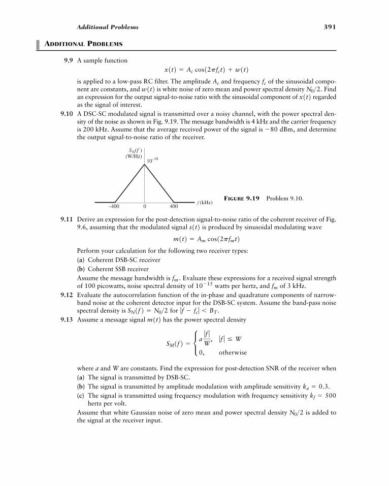
Additional Problems 391
ADDITIONAL PROBLEMS
9.9 A sample function
is applied to a low-pass RC filter. The amplitude and frequency of the sinusoidal compo-nent are constants, and is white noise of zero mean and power spectral density Findan expression for the output signal-to-noise ratio with the sinusoidal component of regardedas the signal of interest.
9.10 A DSC-SC modulated signal is transmitted over a noisy channel, with the power spectral den-sity of the noise as shown in Fig. 9.19. The message bandwidth is 4 kHz and the carrier frequencyis 200 kHz. Assume that the average received power of the signal is and determinethe output signal-to-noise ratio of the receiver.
�80 dBm,
x1t2N0>2.w1t2 fcAc
x1t2 � Ac cos12pfct2 w1t2
10–18
0f (kHz)
–400 400
SN(f )(W/Hz)
FIGURE 9.19 Problem 9.10.
9.11 Derive an expression for the post-detection signal-to-noise ratio of the coherent receiver of Fig.9.6, assuming that the modulated signal is produced by sinusoidal modulating wave
Perform your calculation for the following two receiver types:(a) Coherent DSB-SC receiver(b) Coherent SSB receiverAssume the message bandwidth is Evaluate these expressions for a received signal strengthof 100 picowatts, noise spectral density of watts per hertz, and of 3 kHz.
9.12 Evaluate the autocorrelation function of the in-phase and quadrature components of narrow-band noise at the coherent detector input for the DSB-SC system. Assume the band-pass noisespectral density is for
9.13 Assume a message signal has the power spectral density
where a and W are constants. Find the expression for post-detection SNR of the receiver when(a) The signal is transmitted by DSB-SC.(b) The signal is transmitted by amplitude modulation with amplitude sensitivity (c) The signal is transmitted using frequency modulation with frequency sensitivity
hertz per volt.Assume that white Gaussian noise of zero mean and power spectral density is added tothe signal at the receiver input.
N0>2kf � 500
ka � 0.3.
SM1f2 � c aƒ f ƒW
, ƒ f ƒ � W
0, otherwise
m1t2 ƒ f � fc ƒ � BT .SN1f2 � N0>2
fm10�15fm .
m1t2 � Am cos12pfmt2s1t2
392 CHAPTER 9 � NOISE IN ANALOG COMMUNICATIONS
9.14 A 10 kilowatt transmitter amplitude modulates a carrier with a tone using 50 percent modulation. Propagation losses between the transmitter and the receiver atten-uate the signal by 90 dB. The receiver has a front-end noise with spectral density watts/Hz and includes a bandpass filter with bandwidth What is thepost-detection signal-to-noise ratio, assuming that the receiver uses an envelope detector?
9.15 The average noise power per unit bandwidth measured at the front end of an AM receiver isper Hz. The modulating signal is sinusoidal, with a carrier power of 80 watts and
a sideband power of 10 watts per sideband. The message bandwidth is 4 kHz. Assuming the useof an envelope detector in the receiver, determine the output signal-to-noise ratio of the system.By how many decibels is this system inferior to a DSB-SC modulation system?
9.16 An AM receiver, operating with a sinusoidal modulating wave and 80 percent modulation, hasa post-detection signal-to-noise ratio of 30 dB. What is the corresponding pre-detection signal-to-noise ratio?
9.17 The signal is transmitted via FM. There is an ideal band-pass filter pass-ing at the discriminator output. Calculate the post-detection SNR given that
per volt, and the pre-detection SNR is 500. Use Carson’s rule to estimate the pre-detection bandwidth.
9.18 Suppose that the spectrum of a modulating signal occupies the frequency band To accommodate this signal, the receiver of an FM system (without pre-emphasis) uses an idealband-pass filter connected to the output of the frequency discriminator; the filter passes fre-quencies in the interval Determine the output signal-to-noise ratio and figure ofmerit of the system in the presence of additive white noise at the receiver input.
9.19 An FM system, operating at a pre-detection SNR of 14 dB, requires a post-detection SNR of 30dB, and has a message power of 1 watt and bandwidth of 50 kHz. Using Carson’s rule, estimatewhat the transmission bandwidth of the system must be. Suppose this system includes pre-emphasis and de-emphasis network with of 10 kHz. What transmission bandwidth isrequired in this case?
ADVANCED PROBLEMS
9.20 Assume that the narrowband noise is Gaussian and its power spectral density issymmetric about the midband frequency Show that the in-phase and quadrature compo-nents of are statistically independent.
9.21 Suppose that the receiver bandpass-filter magnitude response has symmetry about and noise bandwidth From the properties of narrowband noise described in Section 8.11,what is the spectral density of the in-phase and quadrature components of the narrow-band noise at the output of the filter? Show that the autocorrelation of is
where justify the approximation for 9.22 Assume that, in the DSB-SC demodulator of Fig. 9.6, there is a phase error in the synchro-
nized oscillator such that its output is Find an expression for the coherentdetector output and show that the post-detection SNR is reduced by the factor
9.23 In a receiver using coherent detection, the sinusoidal wave generated by the local oscillator suf-fers from a phase error with respect to the carrier wave Assuming that isa zero-mean Gaussian process of variance and that most of the time the maximum value of
is small compared to unity, find the mean-square error of the receiver output for DSB-SCmodulation. The mean-square error is defined as the expected value of the squared differencebetween the receiver output and message signal component of a synchronous receiver output.
u1t2 su2
u1t2cos12pfct2.u1t2cos2f.
cos12pfct f2. f
ƒt ƒ V 1>BT .r1t2 � 1r1t2 � F�13SN1f24;RN1t2 � r1t2 cos12pfct2
n1t2n1t2 SN1f2BT .�fcƒHBP1f2 ƒ
n1t2 fc .SN1f2n1t2
f3dB
f1 � ƒ f ƒ � f2 .
f1 � ƒ f ƒ � f2 .
kf � 1 kHz100 � ƒ f ƒ � 300
m1t2 � cos1400pt2
10�6 watts
BT � 2W � 10 kHz.N0 � �113
m1t2 � sin12000pt2,
Computer Experiments 393
9.24 Equation (9.59) is the FM post-detection noise for an ideal low-pass filter. Find the post-detec-tion noise for an FM signal when the post-detection filter is a second-order low-pass filter withmagnitude resonance
Assume for and 9.25 Consider a communication system with a transmission loss of 100 dB and a noise spectral den-
sity of at the receiver input. If the average message power is and thebandwidth is 10 kHz, find the average transmitter power (in kilowatts) required for a post-detection SNR of 40 dB or better when the modulation is:(a) AM with repeat the calculation for (b) FM with 50, and 100 kHz per volt.
In the FM case, check for threshold limitations by confirming that the pre-detection SNR isgreater than 12 dB.
� COMPUTER EXPERIMENTS
9.26 In this experiment, we investigate the performance of amplitude modulation in noise. The MAT-LAB script for AM experiment is provided in Appendix 7, it simulates envelope modulation bya sine wave with a modulation index of 0.3, adds noise, and then envelope-detects the mes-sage. Using this script:(a) Plot the envelope modulated signal.(b) Using the supporting function “spectra,” plot its spectrum.(c) Plot the envelope-detected signal before low-pass filtering.(d) Compare the post-detection SNR to theory.
9.27 In this second computer experiment, we investigate the performance of a FM in noise. Using theMATLAB script for the FM experiment provided in Appendix 7:(a) Plot the spectrum of the baseband FM signal.(b) Plot the spectrum of the band-pass FM plus noise.(c) Plot the spectrum of the detected signal prior to low-pass filtering.(d) Plot the spectrum of the detected signal after low-pass filtering.(e) Compare pre-detection and post-detection SNRs for the FM receiver.
kf � 10,ka � 0.1.ka � 1;
P � 1 watt10�14 W>Hz
BT W 2W.ƒ f ƒ � BT>2ƒHBP1f fc2 ƒ2 � 1
ƒH1f2 ƒ �1
11 1f>W2421>2
394
CHAPTER 10
NOISE IN DIGITAL
COMMUNICATIONS
In the last twenty years, digital communication has been replacing existing analogcommunication in almost every instance. New communication services typically onlyconsider digital communication. There are a number of reasons for this evolution incommunication methods. Two technical reasons are the greater noise tolerance provided bydigital communication, and the almost exact reproducibility of digital sequences at thereceiver. Two strong external reasons for the increased dominance of digital communica-tions are the rapid growth of machine-to-machine communications, such as on the Internet,and the spectacular evolution of digital electronics. In addition, the ability to furtherimprove the robustness of digital communications through the use of error-correction codesis an important advantage over analog. Because digital communications have a greaternoise tolerance than analog, digital communications are applied in situations where analogcommunications would never be. In these demanding situations, noise can still have a signif-icant effect on digital communications, and this is what we will investigate in the chapter.
Broadly speaking, the purpose of detection is to establish the presence or absenceof an information-bearing signal in noise. For this reason, we begin our analysis of theeffects of noise on digital communications by considering the transmission of a singlepulse. The characteristics of noise in digital systems are similar to those in analogsystems; specifically, the received signal may be modeled as
(10.1)
where is the transmitted signal and is the additive noise. As observed in previouschapters, there are numerous similarities between analog and digital modulation tech-niques. We will presently find that there are also similarities between analog and digitalreceiver structures.
The material in this chapter teaches us the following lessons.
� Lesson 1: The bit error rate is the primary measure of performance quality of digitalcommunication systems, and it is typically a nonlinear function of the signal-to-noise ratio.
� Lesson 2: Analysis of single-pulse detection permits a simple derivation of the principleof matched filtering. Matched filtering may be applied to the optimum detection of manylinear digital modulation schemes.
� Lesson 3: The bit error rate performance of binary pulse-amplitude modulation (PAM)improves exponentially with the signal-to-noise ratio in additive white Gaussian noise.
w1t2s1t2r1t2 � s1t2 w1t2
10.1 Bit Error Rate 395
1Speech vocoders analyze the characteristics of short segments of speech, and parameters describing these char-acteristics are transmitted rather than actual samples of the speech. The length of the speech segments is typically20 milliseconds. The advantage of vocoded speech over the PCM techniques described in Chapter 5 is the significantreduction in the bit rate required for an accurate representation. There are a wide variety of speech vocoding algo-rithms, and further details may be found in Gold and Morgan (1999).
� Lesson 4: Receivers for binary and quaternary band-pass linear modulation schemes arestraightforward to develop from matched-filter principles and their performance is similarto binary PAM.
� Lesson 5: Non-coherent detection of digital signals results in a simpler receiver structurebut at the expense of a degradation in bit error rate performance.
� Lesson 6: The provision of redundancy in the transmitted signal through the addition ofparity-check bits may be used for forward-error correction. Forward-error correctionprovides a powerful method to improve the performance of digital modulation schemes.
10.1 Bit Error Rate
With digital systems, it is the output quality of the information that is the primary concern.Since the information is digital and usually has a binary representation, this quality is mea-sured in terms of the average bit error rate (BER). A bit error occurs whenever the trans-mitted bit and the corresponding received bit do not agree; this is a random event. Let ndenote the number of bit errors observed in a sequence of bits of length N; then the rela-tive frequency definition of BER is
(10.2)
In some digital systems, other measures of quality, closely related to the bit error rate, areoften used. For example, many digital systems transfer information in packets and, regard-less of whether there is one error in the packet or a hundred, the whole packet must be dis-carded. In these systems, the measure of quality is often the packet error rate (PER). Thiscan be directly related to the BER if the bit errors are statistically independent.
Naturally, the required bit error rate of a digital system depends upon the application.For example:
� For vocoded speech,1 a BER of to is often considered sufficient.� For data transmission over wireless channels, a bit error rate of to is often
the objective.� For video transmission, a BER of to is often the objective, depending
upon the quality desired and the encoding method.� For financial data, a BER of or better is often the requirement.
Given the availability of different digital modulation–demodulation strategies, we need tocompare their performance. Conceptually, we would like a figure of merit such as we usedwith analog modulation–demodulation systems that we could assign to each digital trans-mission scheme. Unfortunately, that is not as easy to do with digital systems because qual-ity is usually not a linear function of the signal-to-noise ratio.
10�11
10�1210�7
10�610�510�310�2
BER � limNS�
¢ nN≤
396 CHAPTER 10 � NOISE IN DIGITAL COMMUNICATIONS
However, we may define the equivalent of a reference SNR for digital systems. Inparticular, for digital systems, the reference SNR is the ratio of the modulated energy perinformation bit to the one-sided noise spectral density; namely,
This definition differs from the analog definition of reference SNR in three respects.
1. The analog definition was a ratio of powers. The digital definition is a ratio of ener-gies, since the units of noise spectral density are watts/Hz, which is equivalent toenergy. Consequently, the digital definition is dimensionless, as is the analog definition.
2. The definition uses the one-sided noise spectral density; that is, it assumes all of the noiseoccurs on positive frequencies. This assumption is simply a matter of convenience.
3. The reference SNR is independent of transmission rate. Since it is a ratio of energies,it has essentially been normalized by the bit rate.
To compare digital modulation–demodulation strategies, the objective is to deter-mine the bit error rate performance as a function of the reference SNR, denoted by This digital reference model provides a frame of reference for a fair comparison of the dif-ferent schemes.
EXAMPLE 10.1 Computing Packet Error Rate
A transmission system is designed to transfer data with a BER of or better. If this systemis used to transmit packets of 1000 bits, what is the expected packet error rate? Assume thebit errors are statistically independent.
Under the assumption of independent bit errors, the bits in a packet form the equivalentof a Bernoulli sequence. Consequently, the number of bit errors has a binomial distribution asdescribed in Example 8.5. The probability of a packet error is simply one minus the probabil-ity that the packet has no errors; that is, they are complementary events. Consequently, if n isthe number of bit errors, the packet error rate is given by
� Drill Problem 10.1 Let be the event that a 0 is transmitted and let be the eventthat a 0 is received. Define and similarly for a 1. Express the BER in terms of the prob-ability of these events when:(a) The probability of a 1 error is the same as the probability as a 0 error.(b) The probability of a 1 being transmitted is not the same as the probability of a 0 being
transmitted. �
10.2 Detection of a Single Pulse in Noise
With the analog schemes, we saw that it was desirable to make filter bandwidths as smallas possible to minimize the noise, yet not so small that they would distort the desired sig-nal. In a loose sense, we may say that the filters are matched to the signal in a frequency-
R1 ,H1
R0H0
� 9.95 10�3
� 1 � ¢10000≤11 � 10�521000110�520
PER � 1 � Pbinomial1n � 02
10�5
Eb>N0.
�Eb
N0
SNRrefdigital
�Modulated energy per bit
Noise spectral density
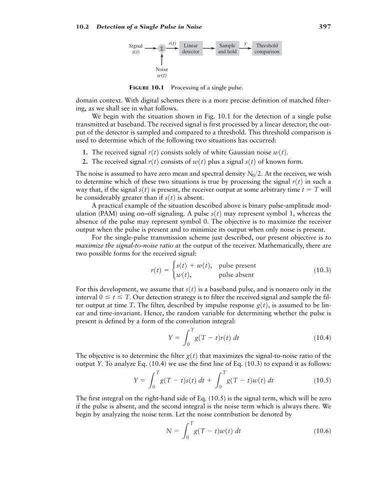
10.2 Detection of a Single Pulse in Noise 397
Lineardetector
Sampleand hold
Thresholdcomparison
Signals(t)
Noisew(t)
r(t) yΣ
FIGURE 10.1 Processing of a single pulse.
domain context. With digital schemes there is a more precise definition of matched filter-ing, as we shall see in what follows.
We begin with the situation shown in Fig. 10.1 for the detection of a single pulsetransmitted at baseband. The received signal is first processed by a linear detector; the out-put of the detector is sampled and compared to a threshold. This threshold comparison isused to determine which of the following two situations has occurred:
1. The received signal consists solely of white Gaussian noise 2. The received signal consists of plus a signal of known form.
The noise is assumed to have zero mean and spectral density At the receiver, we wishto determine which of these two situations is true by processing the signal in such away that, if the signal is present, the receiver output at some arbitrary time willbe considerably greater than if is absent.
A practical example of the situation described above is binary pulse-amplitude mod-ulation (PAM) using on–off signaling. A pulse may represent symbol 1, whereas theabsence of the pulse may represent symbol 0. The objective is to maximize the receiveroutput when the pulse is present and to minimize its output when only noise is present.
For the single-pulse transmission scheme just described, our present objective is tomaximize the signal-to-noise ratio at the output of the receiver. Mathematically, there aretwo possible forms for the received signal:
(10.3)
For this development, we assume that is a baseband pulse, and is nonzero only in theinterval Our detection strategy is to filter the received signal and sample the fil-ter output at time T. The filter, described by impulse response is assumed to be lin-ear and time-invariant. Hence, the random variable for determining whether the pulse ispresent is defined by a form of the convolution integral:
(10.4)
The objective is to determine the filter that maximizes the signal-to-noise ratio of theoutput Y. To analyze Eq. (10.4) we use the first line of Eq. (10.3) to expand it as follows:
(10.5)
The first integral on the right-hand side of Eq. (10.5) is the signal term, which will be zeroif the pulse is absent, and the second integral is the noise term which is always there. Webegin by analyzing the noise term. Let the noise contribution be denoted by
(10.6)N � LT
0g1T � t2w1t2 dt
Y � LT
0g1T � t2s1t2 dt L
T
0g1T � t2w1t2 dt
g1t2Y � L
T
0g1T � t2r1t2 dt
g1t2,0 � t � T.s1t2
r1t2 � b s1t2 w1t2, pulse presentw1t2, pulse absent
s1t2s1t2 t � Ts1t2 r1t2N0>2.
s1t2w1t2r1t2 w1t2.r1t2
398 CHAPTER 10 � NOISE IN DIGITAL COMMUNICATIONS
This sampling of the filter output converts the random process to a random variableN. If the the noise process has units of volts, then Eq. (10.6) can be thought of as aweighted summation of the noise over time, in which case N has units of volt-seconds. Theexpected value of N, defined by
(10.7)
is therefore zero. This result follows from the interchange of expectation and integrationdiscussed in Section 8.9, and the fact that additive white Gaussian noise is assumedto have zero mean. The variance of the output noise is given by
(10.8)
where, once again, we have changed the order of integration and expectation; we are per-mitted to do this because both of these operations are linear. We assume that the noiseprocess is white such that , where is the Dirac deltafunction. Then we may rewrite Eq. (10.8) as
(10.9)
The second line of Eq. (10.9) follows from the first due to the sifting property of the deltafunction. The third line follows from the assumption that the receive filter, has beennormalized; that is,
(10.10)
The units of power spectral density are watts per hertz or watt-seconds. Thus, in Eq.(10.9) has units of if we assume that measurement is performed with aone-ohm resistor, then this is equivalent to This observation shows that theunits of are consistent with those of N. To summarize, the noise sample at the out-put of the linear receiver has
� A mean of zero.� A variance of � A Gaussian distribution, since a filtered Gaussian process is also Gaussian (see Section 8.9).
It should also be noted that other than the normalization constraint of Eq. (10.10), thisanalysis of the noise component has placed no additional constraints on the choice of thefilter impulse response g1t2.
N0T>2.
E3N24 1volt-seconds22.watt-1seconds22;
N0T
LT
0ƒg1t2 ƒ2 dt � T
g1t2,�
N0T
2
�N0
2 LT
0ƒg1T � t2 ƒ2 dt
E3N24 � LT
0 LT
0g1T � t2g1T � t2N0
2d1t � t2 dt dt
d1t2E3w1t2w1t24 � N0>2 d1t � t2
� LT
0 LT
0g1T � t2g1T � t2E3w1t2w1t24 dt dt
� E cLT
0g1T � t2w1t2 dt L
T
0g1T � t2w1t2 dt d
Var1N2 � E3N24w1t2
� 0
E3N4 � LT
0g1T � t2E3w1t24 dt
w1t2 w1t2
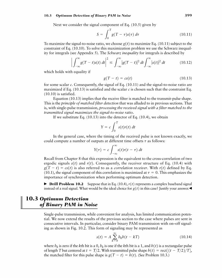
10.3 Optimum Detection of Binary PAM in Noise 399
Next we consider the signal component of Eq. (10.5) given by
(10.11)
To maximize the signal-to-noise ratio, we choose to maximize Eq. (10.11) subject to theconstraint of Eq. (10.10). To solve this maximization problem we use the Schwarz inequal-ity for integrals (see Appendix 5). The Schwarz inequality for integrals is described by
(10.12)
which holds with equality if
(10.13)
for some scalar c. Consequently, the signal of Eq. (10.11) and the signal-to-noise ratio aremaximized if Eq. (10.13) is satisfied and the scalar c is chosen such that the constraint Eq.(10.10) is satisfied.
Equation (10.13) implies that the receive filter is matched to the transmit-pulse shape.This is the principle of matched filter detection that was alluded to in previous sections. Thatis, with single-pulse transmission, processing the received signal with a filter matched to thetransmitted signal maximizes the signal-to-noise ratio.
If we substitute Eq. (10.13) into the detector of Eq. (10.4), we obtain
In the general case, where the timing of the received pulse is not known exactly, wecould compute a number of outputs at different time offsets as follows:
Recall from Chapter 8 that this expression is the equivalent to the cross-correlation of twoergodic signals and Consequently, the receiver structure of Eq. (10.4) with
is also referred to as a correlation receiver. With defined by Eq.(10.1), the signal component of this correlation is maximized at This emphasizes theimportance of synchronization when performing optimum detection.
� Drill Problem 10.2 Suppose that in Eq. (10.4), represents a complex baseband signalinstead of a real signal. What would be the ideal choice for in this case? Justify your answer.�
10.3 Optimum Detection of Binary PAM in Noise
Single-pulse transmission, while convenient for analysis, has limited communication poten-tial. We now extend the results of the previous section to the case where pulses are sent inconsecutive intervals. In particular, consider binary PAM transmission with on–off signal-ing as shown in Fig. 10.2. This form of signaling may be represented as
(10.14)
where is zero if the kth bit is a 0, is one if the kth bit is a 1, and is a rectangular pulseof length T but centered at With transmitted pulse shape the matched filter for this pulse shape is (See Problem 10.3.)g1T � t2 � h1t2. h1t2 � rect31t � T>22>T4,t � T>2.
h1t2bkbk
s1t2 � A aq
k�0bkh1t � kT2
g1t2r1t2t � 0.
r1t2g1T � t2 � cs1t2 r1t2.s1t2Y1t2 � cL
q
�qs1t2r1t � t2 dt
t
Y � cLT
0s1t2r1t2 dt
g1T � t2 � cs1t2
` Lq
�qg1T � t2s1t2 dt ` 2 � L
q
�qƒg1T � t2 ƒ2 dtL
q
�qƒs1t2 ƒ2 dt
g1t2S � L
T
0g1T � t2s1t2 dt
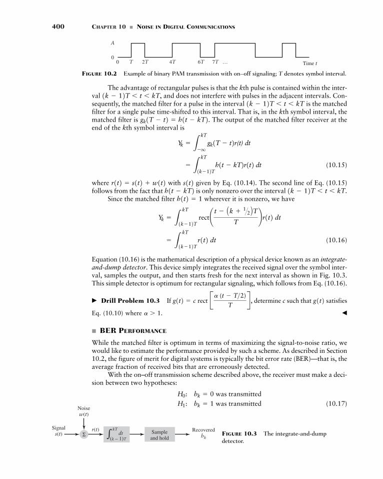
400 CHAPTER 10 � NOISE IN DIGITAL COMMUNICATIONS
A
00 T 2T 4T 6T 7T … Time t
FIGURE 10.2 Example of binary PAM transmission with on–off signaling; T denotes symbol interval.
Σ dtkT
(k – 1)T�
Noisew(t)
Signals(t)
r(t) Recoveredbk
Sampleand hold
The advantage of rectangular pulses is that the kth pulse is contained within the inter-val and does not interfere with pulses in the adjacent intervals. Con-sequently, the matched filter for a pulse in the interval is the matchedfilter for a single pulse time-shifted to this interval. That is, in the kth symbol interval, thematched filter is The output of the matched filter receiver at theend of the kth symbol interval is
(10.15)
where with given by Eq. (10.14). The second line of Eq. (10.15)follows from the fact that is only nonzero over the interval
Since the matched filter wherever it is nonzero, we have
(10.16)
Equation (10.16) is the mathematical description of a physical device known as an integrate-and-dump detector. This device simply integrates the received signal over the symbol inter-val, samples the output, and then starts fresh for the next interval as shown in Fig. 10.3.This simple detector is optimum for rectangular signaling, which follows from Eq. (10.16).
� Drill Problem 10.3 If determine c such that satisfies
Eq. (10.10) where �
� BER PERFORMANCE
While the matched filter is optimum in terms of maximizing the signal-to-noise ratio, wewould like to estimate the performance provided by such a scheme. As described in Section10.2, the figure of merit for digital systems is typically the bit error rate (BER)—that is, theaverage fraction of received bits that are erroneously detected.
With the on–off transmission scheme described above, the receiver must make a deci-sion between two hypotheses:
(10.17)H1: bk � 1 was transmittedH0: bk � 0 was transmitted
a � 1.
g1t2g1t2 � c rect Ba (t � T>2)
TR ,
� LkT
1k�12T r1t2 dt
Yk � LkT
1k�12T rect¢ t � Ak 1�2 BTT
≤r1t2 dt
h1t2 � 11k � 12T � t � kT.h1t � kT2s1t2r1t2 � s1t2 w1t2
� LkT
1k�12Th1t � kT2r1t2 dt
Yk � LkT
�qgk1T � t2r(t) dt
gk1T � t2 � h1t � kT2.1k � 12T � t � kT
1k � 12T � t � kT,
FIGURE 10.3 The integrate-and-dumpdetector.
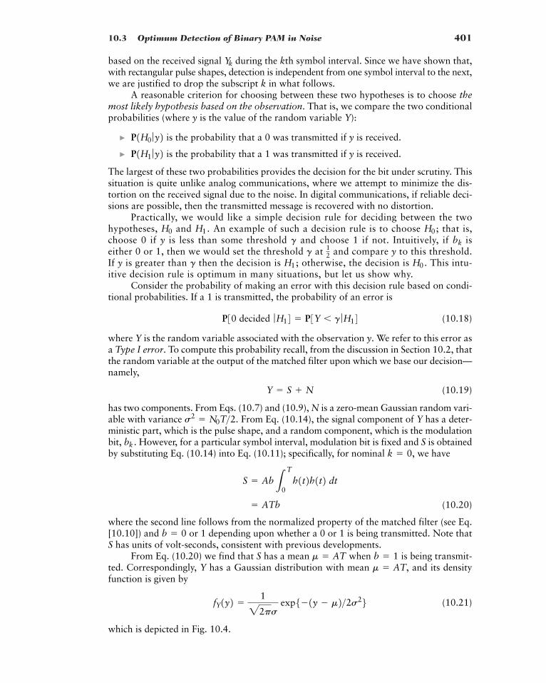
10.3 Optimum Detection of Binary PAM in Noise 401
based on the received signal during the kth symbol interval. Since we have shown that,with rectangular pulse shapes, detection is independent from one symbol interval to the next,we are justified to drop the subscript k in what follows.
A reasonable criterion for choosing between these two hypotheses is to choose themost likely hypothesis based on the observation. That is, we compare the two conditionalprobabilities (where y is the value of the random variable Y):
� is the probability that a 0 was transmitted if y is received.
� is the probability that a 1 was transmitted if y is received.
The largest of these two probabilities provides the decision for the bit under scrutiny. Thissituation is quite unlike analog communications, where we attempt to minimize the dis-tortion on the received signal due to the noise. In digital communications, if reliable deci-sions are possible, then the transmitted message is recovered with no distortion.
Practically, we would like a simple decision rule for deciding between the twohypotheses, and An example of such a decision rule is to choose that is,choose 0 if y is less than some threshold and choose 1 if not. Intuitively, if iseither 0 or 1, then we would set the threshold at and compare y to this threshold.If y is greater than then the decision is otherwise, the decision is This intu-itive decision rule is optimum in many situations, but let us show why.
Consider the probability of making an error with this decision rule based on condi-tional probabilities. If a 1 is transmitted, the probability of an error is
(10.18)
where Y is the random variable associated with the observation y. We refer to this error asa Type I error. To compute this probability recall, from the discussion in Section 10.2, thatthe random variable at the output of the matched filter upon which we base our decision—namely,
(10.19)
has two components. From Eqs. (10.7) and (10.9), N is a zero-mean Gaussian random vari-able with variance From Eq. (10.14), the signal component of Y has a deter-ministic part, which is the pulse shape, and a random component, which is the modulationbit, However, for a particular symbol interval, modulation bit is fixed and S is obtainedby substituting Eq. (10.14) into Eq. (10.11); specifically, for nominal we have
(10.20)
where the second line follows from the normalized property of the matched filter (see Eq.[10.10]) and or 1 depending upon whether a 0 or 1 is being transmitted. Note thatS has units of volt-seconds, consistent with previous developments.
From Eq. (10.20) we find that S has a mean when is being transmit-ted. Correspondingly, Y has a Gaussian distribution with mean and its densityfunction is given by
(10.21)
which is depicted in Fig. 10.4.
fY1y2 �1
22ps exp5�1y � m2>2s26
m � AT,b � 1m � AT
b � 0
� ATb
S � AbLT
0h1t2h1t2 dt
k � 0,bk .
s2 � N0T>2.
Y � S N
P30 decided ƒH14 � P3Y � g ƒH14
H0.H1;g
12g
bkg
H0;H1.H0
P1H1 ƒy2P1H0 ƒy2
Yk
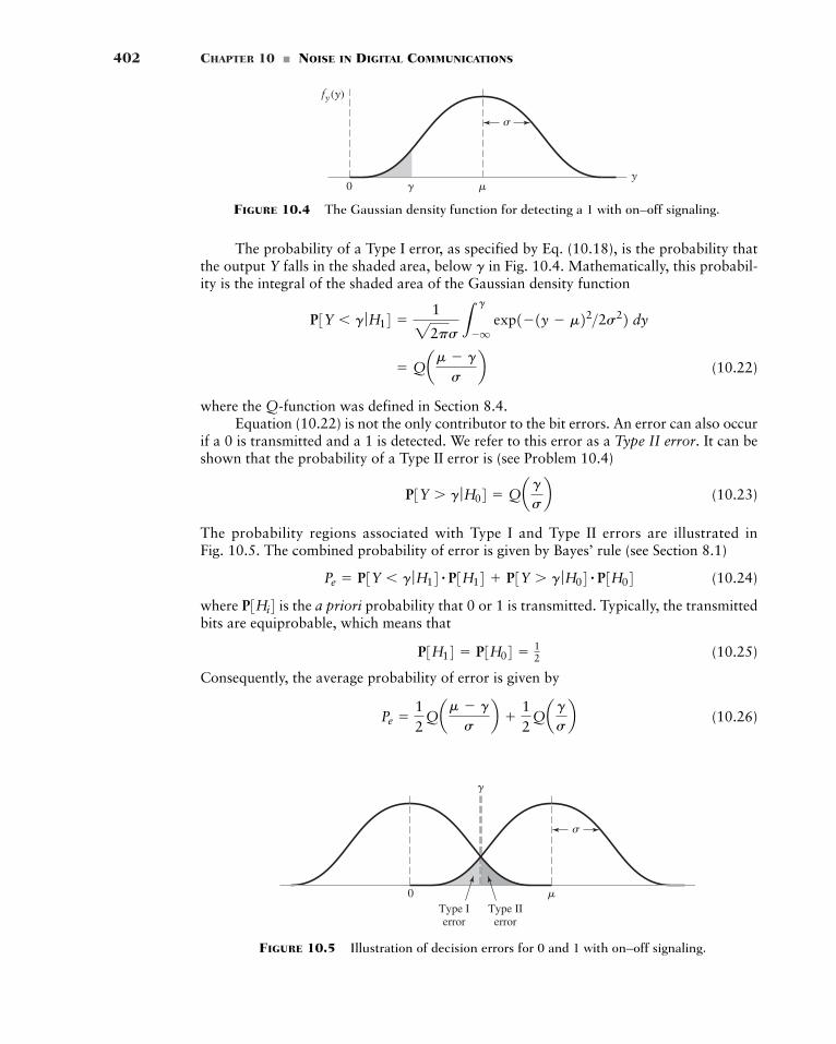
402 CHAPTER 10 � NOISE IN DIGITAL COMMUNICATIONS
0 �
Type Ierror
Type IIerror
FIGURE 10.5 Illustration of decision errors for 0 and 1 with on–off signaling.
0 �y
fy (y)
FIGURE 10.4 The Gaussian density function for detecting a 1 with on–off signaling.
The probability of a Type I error, as specified by Eq. (10.18), is the probability thatthe output Y falls in the shaded area, below in Fig. 10.4. Mathematically, this probabil-ity is the integral of the shaded area of the Gaussian density function
(10.22)
where the Q-function was defined in Section 8.4.Equation (10.22) is not the only contributor to the bit errors. An error can also occur
if a 0 is transmitted and a 1 is detected. We refer to this error as a Type II error. It can beshown that the probability of a Type II error is (see Problem 10.4)
(10.23)
The probability regions associated with Type I and Type II errors are illustrated in Fig. 10.5. The combined probability of error is given by Bayes’ rule (see Section 8.1)
(10.24)
where is the a priori probability that 0 or 1 is transmitted. Typically, the transmittedbits are equiprobable, which means that
(10.25)
Consequently, the average probability of error is given by
(10.26)Pe �12
Qam � g
sb
12
Qa gsb
P3H14 � P3H04 � 12
P3Hi4Pe � P3Y � g ƒH14 # P3H14 P3Y � g ƒH04 # P3H04
P3Y � g ƒH04 � Qa gsb
� Qam � g
sb
P3Y � g ƒH14 �1
22ps Lg
�q exp1�1y � m22>2s22 dy
g
10.3 Optimum Detection of Binary PAM in Noise 403
Often we would like the probabilities of the two types of errors, P[Type I error] andP[Type II error], to be equal; so we choose It can be shown that this choice of minimizes the probability of error described by Eq. (10.26) (see Problem 10.22). Conse-quently, we have that the average probability of error is given by
(10.27)
That is, the probability of a bit error depends upon the ratio of the signal mean when 1is transmitted to the noise standard deviation through the nonlinear function Q.
Our next step is to express this probability of bit error in terms of the digital refer-ence model. This evaluation may be broken down into two components:
� To express the variance in terms of the noise spectral density, we have, from Eq.(10.9), that
� To express the signal amplitude in terms of the energy per bit we assume that0 and 1 are equally likely to be transmitted. Then the average energy per bit at thereceiver input is
(10.28)
where, in the second line, we have separated the deterministic and random parts ofthe signal and the third line follows from the fact that Consequently, we have that for the case of on-off PAM signaling.
By substituting these values for and into Eq. (10.27), the result obtained is
(10.29)
It is interesting to note that if, instead of on–off keying with levels of 0 and A, we usedbipolar levels of and then the above analysis would be unchanged exceptthat the threshold would now be However, with the bipolar scheme the energy perbit is and the bit error rate in terms of the digital reference model is
(10.30)
Since the Q-function is a monotone decreasing function of its argument, Eq. (10.30) impliesthat a smaller ratio will produce the same error rate as the on–off scheme charac-terized by Eq. (10.29). Thus, we find that bipolar signaling is a more power-efficient methodof achieving the same bit error rate performance than the on–off signaling scheme.
� Drill Problem 10.4 Show that with on-off signaling, the probability of a Type II errorin Eq. (10.23) is given by
�P3Y � g ƒH04 � Qa gsb
Eb>N0
Pebipolar � Q¢A2Eb
N0≤Eb � A2T>4,
g � 0.A>2,�A>2
Peon–off � Q¢AEb
N0≤m � ATs
A � 22Eb>T h1t2 � rect31t � T>22>T4.�
A2T2
� A2e 12# 0
12# 1 fT
� A2E3b24LT
0ƒh1t2 ƒ2 dt
Eb � E cLT
0ƒs1t2 ƒ2 dt d
Eb ,As2 � N0T>2.
s
m
Pe � Qa m2sb
gg � m>2.
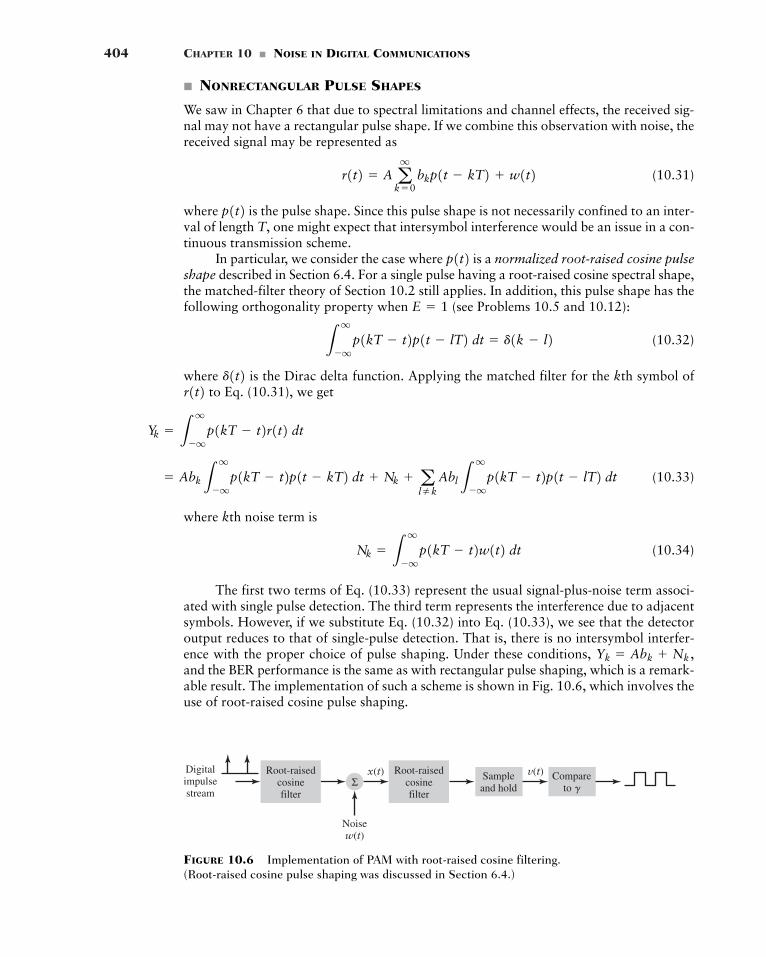
404 CHAPTER 10 � NOISE IN DIGITAL COMMUNICATIONS
� NONRECTANGULAR PULSE SHAPES
We saw in Chapter 6 that due to spectral limitations and channel effects, the received sig-nal may not have a rectangular pulse shape. If we combine this observation with noise, thereceived signal may be represented as
(10.31)
where is the pulse shape. Since this pulse shape is not necessarily confined to an inter-val of length T, one might expect that intersymbol interference would be an issue in a con-tinuous transmission scheme.
In particular, we consider the case where is a normalized root-raised cosine pulseshape described in Section 6.4. For a single pulse having a root-raised cosine spectral shape,the matched-filter theory of Section 10.2 still applies. In addition, this pulse shape has thefollowing orthogonality property when (see Problems 10.5 and 10.12):
(10.32)
where is the Dirac delta function. Applying the matched filter for the kth symbol ofto Eq. (10.31), we get
(10.33)
where kth noise term is
(10.34)
The first two terms of Eq. (10.33) represent the usual signal-plus-noise term associ-ated with single pulse detection. The third term represents the interference due to adjacentsymbols. However, if we substitute Eq. (10.32) into Eq. (10.33), we see that the detectoroutput reduces to that of single-pulse detection. That is, there is no intersymbol interfer-ence with the proper choice of pulse shaping. Under these conditions, and the BER performance is the same as with rectangular pulse shaping, which is a remark-able result. The implementation of such a scheme is shown in Fig. 10.6, which involves theuse of root-raised cosine pulse shaping.
Yk � Abk Nk ,
Nk � Lq
�qp1kT � t2w1t2 dt
� AbkLq
�qp1kT � t2p1t � kT2 dt Nk a
lkAblL
q
�qp1kT � t2p1t � lT2 dt
Yk � Lq
�qp1kT � t2r1t2 dt
r1t2 d1t2L
q
�qp1kT � t2p1t � lT2 dt � d1k � l2
E � 1
p1t2p1t2
r1t2 � A aq
k�0bkp1t � kT2 w1t2
Sampleand hold
Compareto
Noisew(t)
x(t) v(t)Σ
Root-raisedcosinefilter
Root-raisedcosinefilter
Digitalimpulsestream
FIGURE 10.6 Implementation of PAM with root-raised cosine filtering. (Root-raised cosine pulse shaping was discussed in Section 6.4.)
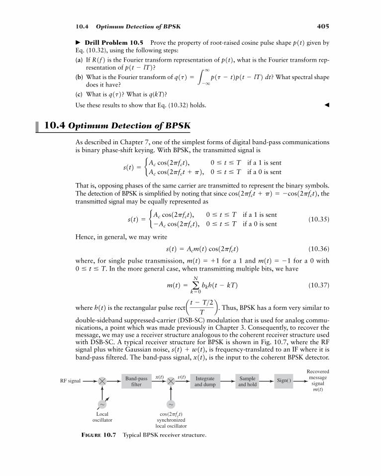
10.4 Optimum Detection of BPSK 405
� Drill Problem 10.5 Prove the property of root-raised cosine pulse shape given byEq. (10.32), using the following steps:
(a) If is the Fourier transform representation of what is the Fourier transform rep-resentation of
(b) What is the Fourier transform of What spectral shapedoes it have?
(c) What is What is q(kT)?
Use these results to show that Eq. (10.32) holds. �
10.4 Optimum Detection of BPSK
As described in Chapter 7, one of the simplest forms of digital band-pass communicationsis binary phase-shift keying. With BPSK, the transmitted signal is
That is, opposing phases of the same carrier are transmitted to represent the binary symbols.The detection of BPSK is simplified by noting that since thetransmitted signal may be equally represented as
(10.35)
Hence, in general, we may write
(10.36)
where, for single pulse transmission, for a 1 and for a 0 withIn the more general case, when transmitting multiple bits, we have
(10.37)
where is the rectangular pulse Thus, BPSK has a form very similar to
double-sideband suppressed-carrier (DSB-SC) modulation that is used for analog commu-nications, a point which was made previously in Chapter 3. Consequently, to recover themessage, we may use a receiver structure analogous to the coherent receiver structure usedwith DSB-SC. A typical receiver structure for BPSK is shown in Fig. 10.7, where the RFsignal plus white Gaussian noise, is frequency-translated to an IF where it isband-pass filtered. The band-pass signal, is the input to the coherent BPSK detector.x1t2,s1t2 w1t2,
recta t � T>2T
b .h1t2m1t2 � a
N
k�0bkh1t � kT2
0 � t � T.m1t2 � �1m1t2 � 1
s1t2 � Acm1t2 cos12pfct2
s1t2 � bAc cos12pfct2, 0 � t � T if a 1 is sent�Ac cos12pfct2, 0 � t � T if a 0 is sent
cos12pfct p2 � �cos12pfct2,
s1t2 � bAc cos12pfct2, 0 � t � T if a 1 is sentAc cos12pfct p2, 0 � t � T if a 0 is sent
q1t2?q1t2 � L
q
�qp1t � t2p1t � lT2 dt?
p1t � lT2? p1t2,R1f2p1t2
FIGURE 10.7 Typical BPSK receiver structure.
~
Recoveredmessagesignalm(t)
RF signal
~
x(t) v(t) Integrateand dump
Band-passfilter
Localoscillator
cos(2�fct)synchronized
local oscillator
Sampleand hold
Sign( )
406 CHAPTER 10 � NOISE IN DIGITAL COMMUNICATIONS
� DETECTION OF BPSK IN NOISE
Following the development for DSB-SC demodulation of Section 9.4, the signal plus band-pass noise at the input to the coherent BPSK detector of Fig. 10.7 may be represented as
(10.38)
where and are the in-phase and quadrature components of the band-pass noiserespectively. The output of the product modulator in Fig. 10.7 is given by
(10.39)
where we have used the double angle formulas: cos Aand sin A Let us consider the two parts of the sec-ond line of Eq. (10.39). The first part represents the baseband signal plus a baseband com-ponent of the noise, while the second part represents signal and noise centered at the muchhigher frequency of
With the analog DSB-SC signal, we used a low-pass filter to remove the high-fre-quency noise components and recover the desired signal. With digital signals, we knowthat a matched filter is the optimum method to recover the data. We could combine thematched filter with a low-pass filter to achieve the desired results, as long as the low-passfilter does not distort the desired signal. However, if we recognize that the matched filter
is already a low-pass filter, then there is no need for the second filter.The observant reader will note that in the derivation of the matched filter, we assume
that the noise is white. The in-phase component is narrowband noise and hence notwhite. However, it can be shown that as long as the bandpass filter has a wider bandwidththan that of the signal and the noise spectral density is approximately flat over the band-width of the signal, the matched-filter principle still applies.
In the case where consists of rectangular pulses, the optimum detector after down-conversion is the integrate-and-dump filter, as was shown for the case of pulse-amplitudemodulation (PAM). The output of the integrate-and-dump detector in this case is therefore
(10.40)
Equation (10.40) assumes that the high-frequency terms have negligible impact on thedetector output. The noise term in Eq. (10.40) is given by
(10.41)
Recall from Section 8.11 that if the power spectral density of the narrowband noise is then the power spectral density of the in-phase component of the noise is over their respective frequency bands. Accordingly, we may write
N0,nI1t2N0>2,n1t2
Nk �12 L
kT
1k�12T nI1t2 dt
�AcT
2bk Nk
Yk �12 L
kT
1k�12T 3Acm1t2 nI1t24 dt
m1t2
nI1t2
� recta t � T>2T
bg1T � t2 � h1t2
2fc .
cos B � 125sin1A � B2 sin1A B26. cos B � 1
25cos1A � B2 cos1A B26� 1
2 CAcm1t2 nI1t2D C121Acm1t2 nI1t22 cos14pfct2 � 12 nQ1t2 sin14pfct2Dv1t2 � x1t2 cos12pfct2
n1t2, nQ1t2nI1t2x1t2 � s1t2 nI1t2 cos12pfct2 � nQ1t2 sin12pfct2
10.4 Optimum Detection of BPSK 407
Thus, the variance of in Eq. (10.41) is In Fig. 7.4(b), we show a BPSK demodulator quite similar to that shown in Fig. 10.7.
The main difference between the two demodulators is that the low-pass filter of the formeris replaced by the integrator of the latter. In the noiseless case of Chapter 7, the purpose ofthe low-pass filter is to remove the high-frequency components, while retaining the desiredbaseband signal. The integrator of Fig. 10.7 also acts as a low-pass filter removing the high-frequency components but, due to its matched property, it additionally removes as much noiseas possible from the signal, and thereby maximizes the signal-to-noise ratio at the demod-ulator output. Note that in digital communications, the objective is to recover the informa-tion, 0s and 1s, as reliably as possible. Unlike analog communications, there is no requirementthat the transmitted waveform should be recovered with minimum distortion.
� PERFORMANCE ANALYSIS
The bit error rate analysis with BPSK is similar to the analysis of bipolar signaling in Section10.3. The threshold for deciding between a 0 and a 1 at the output of the matched filter isset at zero. A threshold of zero has the practical advantage that it does not have to be cal-ibrated if the transmission path has an unknown gain.
From Eq. (10.40), the mean signal value is or depending uponwhether is or respectively. If we assume a 1 was transmitted and let then the probability of error is
(10.42)
Consequently, analogous to Eq. (10.22) with the bit error rate is given by
(10.43)
By symmetry, this result holds when either a or is transmitted. In terms of the dig-ital reference model, we note that the energy per bit with BPSK, assuming the energy of thepulses in is normalized, is simply Using this result in the definition of
with we have
m �AcT
2� A2Eb
TT2
� AEbT
2
bk � 1,m,Eb � Ac
2T>2.m1t2�11
Pe � Qamsb
g � 0,
�1
22ps L0
�q expb�1y � m22
2s2 r dy
Pe � P3Y � 04m � AcT>2,�1,1bk
�AcT>2,AcT>2
14 N0T.Nks2
�N0T
4
�14 L
kT
1k�12T N0 ds
�14cL
kT
1k�12TLkT
1k�12T N0d1t � s2 dt ds dE3Nk
24 �14
E cLkT
1k�12TLkT
1k�12T nI1t2nI1s2 dt ds d
408 CHAPTER 10 � NOISE IN DIGITAL COMMUNICATIONS
Substituting the value of so obtained and into Eq. (10.43), we obtain theresult
(10.44)
This BER performance is exactly the same as that of the baseband bipolar scheme as givenin Eq. (10.30). That is, there is no difference in BER performance between the low-pass bipo-lar PAM signaling and bandpass BPSK modulation. Thus, just as in the analog case, thereis no change in the figure of merit when we go from a baseband system to an equivalentcoherent band-pass system.
The analysis of BPSK can be extended to nonrectangular pulse shaping in a mannersimilar to what occurred at baseband. For nonrectangular pulse shaping, we represent thetransmitted signal as
(10.45)
where is the pulse shape and represents the data. This combination of pulseshaping and BPSK modulation forms an important method of communicating binary infor-mation and controlling the bandwidth required for the transmission. In particular, BPSKmodulation allows multiple users to use the same transmission medium by choosing car-rier frequencies and the pulse shaping limits the transmitted signal bandwidth and thusreduces or eliminates the interference between communication links using different
� Drill Problem 10.6 Compare the transmission bandwidth required for binary PAMand BPSK modulation, if both signals have a data rate of 9600 bps and use root-raised cosinepulse spectrum with a roll-off factor of 0.5. �
� Drill Problem 10.7 Sketch a block diagram of a transmission system including bothtransmitter and receiver for BPSK modulation with root-raised cosine pulse shaping. �
10.5 Detection of QPSK and QAM in Noise
With an understanding of binary data detection in noise for both the baseband (PAM) andpassband (BPSK) at our disposal, we now extend these results to more complex modula-tion schemes such as quadri-phase-shift keying (QPSK) and quadrature amplitude modu-lation (QAM).
� DETECTION OF QPSK IN NOISE
We saw in Section 7.3 that QPSK-modulated signal could be represented in the form
(10.46)
for The carrier is transmitted in one of four phases with each phase represent-ing a two-bit pair (i.e., dibit), as given by
0 � t � T.
s1t2 � Ac cos12pfct f1t22s1t2
fc .fc ;
bk � �1p1t2s1t2 � Ac a
q
k��qbkp1t � kT2 cos12pfct2
PeBPSK � Q¢A2Eb
N0≤
s � 122N0Tm
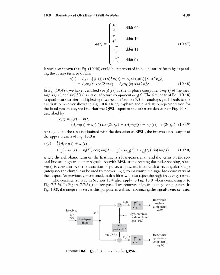
10.5 Detection of QPSK and QAM in Noise 409
Recoveredquadraturecomponent
–mQ(t)
vQ(t)sin(2�fct)
dtT
0�
v1(t)
Receivedsignalr(t)
x(t)
Recoveredin-phase
componentmI(t)
Synchronizedlocal oscillator
cos(2�fct)Band-passfilter
dtT
0�
–90°phase shift
FIGURE 10.8 Quadrature receiver for QPSK.
(10.47)
It was also shown that Eq. (10.46) could be represented in a quadrature form by expand-ing the cosine term to obtain
(10.48)
In Eq. (10.48), we have identified as the in-phase component of the mes-sage signal, and as its quadrature component The similarity of Eq. (10.48)to quadrature-carrier multiplexing discussed in Section 3.5 for analog signals leads to thequadrature receiver shown in Fig. 10.8. Using in-phase and quadrature representation forthe band-pass noise, we find that the QPSK input to the coherent detector of Fig. 10.8 isdescribed by
(10.49)
Analogous to the results obtained with the detection of BPSK, the intermediate output ofthe upper branch of Fig. 10.8 is
(10.50)
where the right-hand term on the first line is a low-pass signal; and the terms on the sec-ond line are high-frequency signals. As with BPSK using rectangular pulse shaping, since
is constant over the duration of pulse, a matched filter with a rectangular shape(integrate-and-dump) can be used to recover to maximize the signal-to-noise ratio ofthe output. As previously mentioned, such a filter will also reject the high-frequency terms.
The comments made in Section 10.4 also apply to Fig. 10.8 when comparing it toFig. 7.7(b). In Figure 7.7(b), the low-pass filter removes high-frequency components. InFig. 10.8, the integrator serves this purpose as well as maximizing the signal-to-noise ratio.
mI1t2mI1t2
12 1AcmI1t2 nI1t22 cos14pfct2 � 1
2 1AcmQ1t2 nQ1t22 sin14pfct2vI1t2 � 1
2 1AcmI1t2 nI1t22
� 1AcmI1t2 nI1t22 cos12pfct2 � 1AcmQ1t2 nQ1t22 sin12pfct2x1t2 � s1t2 n1t2
mQ1t2.sin3f1t24 mI1t2cos3f1t24� AcmI1t2 cos12pfct2 � AcmQ1t2 sin12pfct2
s1t2 � Ac cos3f1t24 cos12pfct2 � Ac sin3f1t24 sin12pfct2
f1t2 � h3p4
, dibit 00
p
4, dibit 10
�p
4, dibit 11
�3p4
, dibit 01
410 CHAPTER 10 � NOISE IN DIGITAL COMMUNICATIONS
Similarly, the output of the lower branch of the quadrature detector is
(10.51)
The baseband signal can be recovered in a manner similar to For the in-phase component, if the first bit of the dibit is a 0, then the mean output is
If on the other hand, the first bit of the dibit is a 1 then
After low-pass filtering, the form of Eq. (10.50) is the same as we found with BPSK in Eq.(10.40). Consequently, the probability of error on the in-phase branch of the QPSK signal is
(10.52)
where is the square root of the noise variance (i.e. the standard deviation). The indi-cates the symmetry between the 0 bit and the 1 bit. The same result holds for the quadra-ture component. To express this result in terms of the digital reference model we note that,with QPSK modulation, two bits are transmitted in one symbol interval of length T. Con-sequently, the average energy by bit may be determined from
(10.53)
where, under the bandpass assumption, the integral of the high-frequency term is approx-imately zero. We also note that the noise variance at each branch output is unchanged fromBPSK with With this difference, the bit error rate with after matched fil-tering is given by
(10.54)� Q ¢A2Eb
N0≤
� Q ¢ AcT�222
21�4 N0T≤Pe
QPSK � Qa ƒm ƒsb
vI1t2s2 � 14 N0T.
�Ac
2T
2
� Ac2
LT
0
1 cos14pfct 2f1t222
dt
� Ac2
LT
0 cos212pfct f1t22 dt
2Eb � E cLT
0s21t2 dt d
ƒm ƒs
Pe � Qa ƒm ƒsb
m �AcT
2cosa�p
4b �
AcT
222
m �AcT
2cosa�3p
4b � �
AcT
222
mI1t2.mQ1t2 1
2 1AcmQ1t2 nQ1t22 cos14pfct2 12 1AcmI1t2 nI1t22 sin14pfct2
vQ1t2 � �12 1AcmQ1t2 nQ1t22
10.5 Detection of QPSK and QAM in Noise 411
where we have made the substitution from Eq. (10.53). A similar resultfollows for by symmetry.
Consequently, in terms of energy per bit, the QPSK performance is exactly the sameas BPSK, even though we are transmitting twice as many bits through the same channel.This important result is due to the inherent orthogonal nature of the in-phase and quad-rature components. Once again we may draw an analogy with analog communications,where comparing double-sideband and single-sideband transmission, we found that wecould obtain the same quality of performance but with half of the transmission bandwidth.With QPSK modulation, we use the same transmission bandwidth as BPSK but transmittwice as many bits with the same reliability.
As described in Section 7.3, offset-QPSK or OQPSK is a variant of QPSK modulationwherein the quadrature component is delayed by one-half of symbol period relative to thein-phase component. Under the bandpass assumption, delaying the quadrature componentdoes not change its orthogonality with the in-phase component. Consequently, we mayuse the same quadrature detector for recovering an OQPSK as is used for QPSK. The onlydifference is that the sampling of the integrate-and-dump detector of the quadrature com-ponent occurs one-half symbol latter than that for the in-phase component.
As a result of this similarity between the OQPSK and QPSK, the bit error rate per-formance of both schemes is identical if the transmission path does not distort the signal.As mentioned in Chapter 7, one advantage of OQPSK is its reduced phase variations andpotentially less distortion if the transmission path includes nonlinear components such asan amplifier operating near or at saturation. Under such nonlinear conditions, OQPSKmay perform better than QPSK.
� Drill Problem 10.8 Show that the integral of the high-frequency term in Eq. (10.53) isapproximately zero. �
� DETECTION OF QAM IN NOISE
Quadrature amplitude modulation (QAM), discussed in Section 7.7, is also a band-passmodulation strategy due to its use of the in-phase and quadrature components of the car-rier. QAM can be viewed as a hybrid of multi-level PAM and QPSK. In particular, QAMuses in-phase and quadrature components for transmission just as QPSK does. However,in each of the in-phase and quadrature components in QAM, the modulator uses multiplelevels—that is, more than the two levels of or used in QPSK.
First, let us consider multi-level PAM. Let the baseband modulated signal be repre-sented by
(10.55)
where the represent different modulation levels. For example, with four-level PAM, thescalar could be selected from the set The eye diagram for such amulti-level signal could look like Fig. 10.9.
If we review the analysis of the optimum procedure that led to the matched filterdetector, we find that it did not depend on the signal amplitude. Consequently, the detec-tor design for the multi-level PAM receiver is identical to that for on–off PAM. The onlydifference between binary PAM and multi-level PAM is the threshold comparisons used todetermine which of the levels were transmitted, as depicted in Fig. 10.10.
5�3, �1, 1, 36.ck
ck
s1t2 � A aq
k�0ckh1t � kT2
�sin f�cos f
vQ1t2 Ac � 24Eb>T
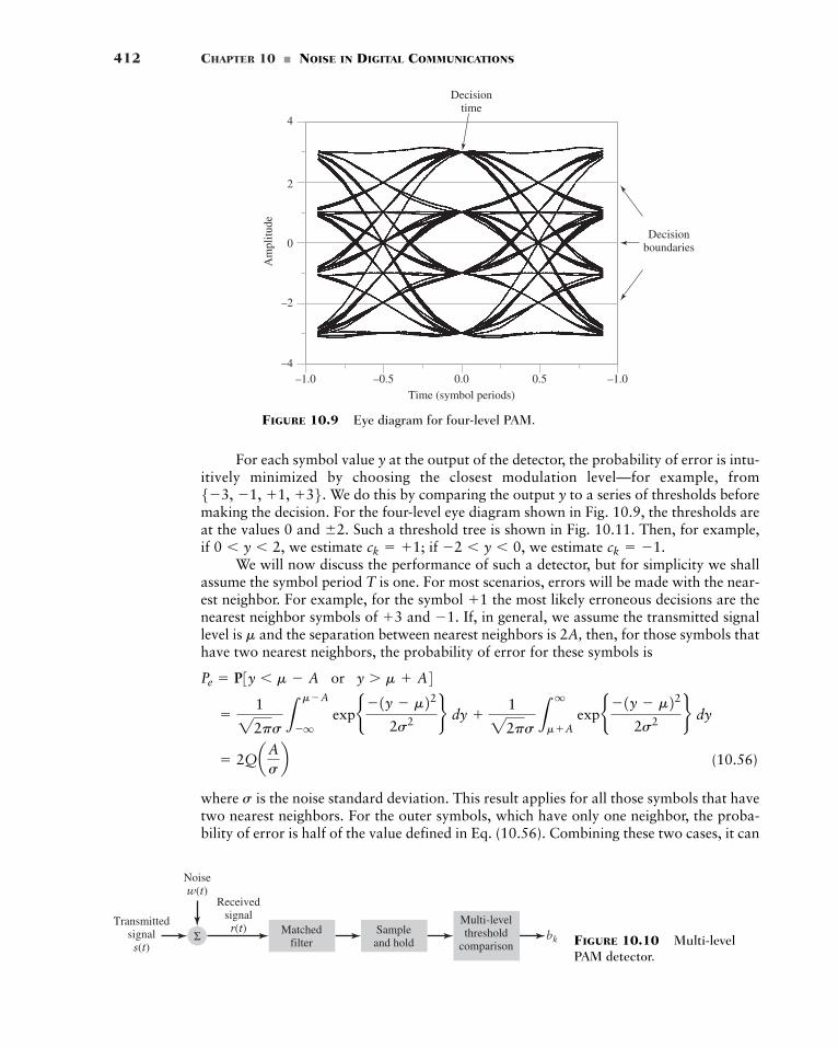
412 CHAPTER 10 � NOISE IN DIGITAL COMMUNICATIONS
Am
plitu
de
–1.0 –0.5 0.0Time (symbol periods)
Decisiontime
Decisionboundaries
0.5 –1.0–4
–2
0
2
4
FIGURE 10.9 Eye diagram for four-level PAM.
For each symbol value y at the output of the detector, the probability of error is intu-itively minimized by choosing the closest modulation level—for example, from
We do this by comparing the output y to a series of thresholds beforemaking the decision. For the four-level eye diagram shown in Fig. 10.9, the thresholds areat the values 0 and Such a threshold tree is shown in Fig. 10.11. Then, for example,if we estimate if we estimate
We will now discuss the performance of such a detector, but for simplicity we shallassume the symbol period T is one. For most scenarios, errors will be made with the near-est neighbor. For example, for the symbol the most likely erroneous decisions are thenearest neighbor symbols of and If, in general, we assume the transmitted signallevel is and the separation between nearest neighbors is 2A, then, for those symbols thathave two nearest neighbors, the probability of error for these symbols is
(10.56)
where is the noise standard deviation. This result applies for all those symbols that havetwo nearest neighbors. For the outer symbols, which have only one neighbor, the proba-bility of error is half of the value defined in Eq. (10.56). Combining these two cases, it can
s
� 2QaAsb
�1
22ps Lm�A
�q expb�1y � m22
2s2 r dy 1
22ps Lq
mA expb�1y � m22
2s2 r dy
Pe � P3y � m � A or y � m A4m
�1.31
ck � �1.�2 � y � 0,ck � 1;0 � y � 2,�2.
5�3, �1, 1, 36.
bkΣ
Noisew(t)
Transmittedsignals(t)
Receivedsignalr(t) Sample
and holdMatched
filter
Multi-levelthreshold
comparison FIGURE 10.10 Multi-levelPAM detector.
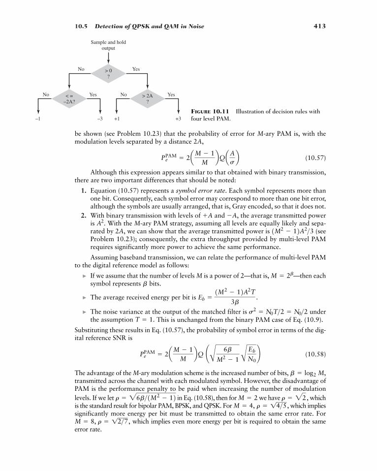
10.5 Detection of QPSK and QAM in Noise 413
Sample and holdoutput
–1 –3 +1 +3
No Yes
No YesNo Yes
> 0?
< =–2A?
> 2A?
FIGURE 10.11 Illustration of decision rules withfour level PAM.
be shown (see Problem 10.23) that the probability of error for M-ary PAM is, with themodulation levels separated by a distance 2A,
(10.57)
Although this expression appears similar to that obtained with binary transmission,there are two important differences that should be noted:
1. Equation (10.57) represents a symbol error rate. Each symbol represents more thanone bit. Consequently, each symbol error may correspond to more than one bit error,although the symbols are usually arranged, that is, Gray encoded, so that it does not.
2. With binary transmission with levels of and the average transmitted poweris With the M-ary PAM strategy, assuming all levels are equally likely and sepa-rated by 2A, we can show that the average transmitted power is (seeProblem 10.23); consequently, the extra throughput provided by multi-level PAMrequires significantly more power to achieve the same performance.
Assuming baseband transmission, we can relate the performance of multi-level PAMto the digital reference model as follows:
� If we assume that the number of levels M is a power of 2—that is, —then eachsymbol represents bits.
� The average received energy per bit is
� The noise variance at the output of the matched filter is underthe assumption This is unchanged from the binary PAM case of Eq. (10.9).
Substituting these results in Eq. (10.57), the probability of symbol error in terms of the dig-ital reference SNR is
(10.58)
The advantage of the M-ary modulation scheme is the increased number of bits, transmitted across the channel with each modulated symbol. However, the disadvantage ofPAM is the performance penalty to be paid when increasing the number of modulation levels. If we let in Eq. (10.58), then for we have whichis the standard result for bipolar PAM, BPSK, and QPSK. For which impliessignificantly more energy per bit must be transmitted to obtain the same error rate. For
which implies even more energy per bit is required to obtain the sameerror rate.M � 8, r � 12>7,
M � 4, r � 14>5,r � 22,M � 2r � 26b>1M2 � 12
b � log2 M,
PePAM � 2aM � 1
MbQ ¢A 6b
M2 � 1 A Eb
N0≤
T � 1.s2 � N0T>2 � N0>2
Eb �1M2 � 12A2T
3b.
b
M � 2b
1M2 � 12A2>3A2.�A,A
PePAM � 2aM � 1
MbQaA
sb
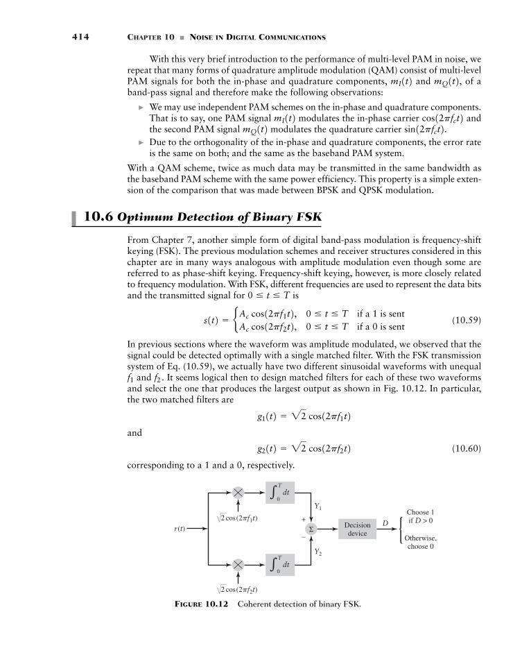
414 CHAPTER 10 � NOISE IN DIGITAL COMMUNICATIONS
With this very brief introduction to the performance of multi-level PAM in noise, werepeat that many forms of quadrature amplitude modulation (QAM) consist of multi-levelPAM signals for both the in-phase and quadrature components, and of aband-pass signal and therefore make the following observations:
� We may use independent PAM schemes on the in-phase and quadrature components.That is to say, one PAM signal modulates the in-phase carrier andthe second PAM signal modulates the quadrature carrier
� Due to the orthogonality of the in-phase and quadrature components, the error rateis the same on both; and the same as the baseband PAM system.
With a QAM scheme, twice as much data may be transmitted in the same bandwidth asthe baseband PAM scheme with the same power efficiency. This property is a simple exten-sion of the comparison that was made between BPSK and QPSK modulation.
10.6 Optimum Detection of Binary FSK
From Chapter 7, another simple form of digital band-pass modulation is frequency-shiftkeying (FSK). The previous modulation schemes and receiver structures considered in thischapter are in many ways analogous with amplitude modulation even though some arereferred to as phase-shift keying. Frequency-shift keying, however, is more closely relatedto frequency modulation. With FSK, different frequencies are used to represent the data bitsand the transmitted signal for is
(10.59)
In previous sections where the waveform was amplitude modulated, we observed that thesignal could be detected optimally with a single matched filter. With the FSK transmissionsystem of Eq. (10.59), we actually have two different sinusoidal waveforms with unequal
and It seems logical then to design matched filters for each of these two waveformsand select the one that produces the largest output as shown in Fig. 10.12. In particular,the two matched filters are
and
(10.60)
corresponding to a 1 and a 0, respectively.
g21t2 � 22 cos12pf2t2g11t2 � 22 cos12pf1t2
f2.f1
s1t2 � bAc cos12pf1t2, 0 � t � T if a 1 is sentAc cos12pf2t2, 0 � t � T if a 0 is sent
0 � t � T
sin12pfct2.mQ1t2 cos12pfct2mI1t2
mQ1t2,mI1t2
r(t)cos(2�f1t)
Y1
Y2
+
–
Decisiondevice
Choose 1if D > 0
Otherwise,choose 0
D
dtT
0�
dtT
0�
Σ/2
cos(2�f2t)/2FIGURE 10.12 Coherent detection of binary FSK.
10.6 Optimum Detection of Binary FSK 415
To analyze the performance of the FSK detector of Fig. 10.12, we make the simpli-fying assumption that the frequencies and have been selected such that the corre-sponding waveforms are orthogonal; that is,
(10.61)
Technically, this implies that is an integer under the bandpass assumption (seeProblem 10.16). This assumption is not necessary in practice, but violation of this assump-tion does result in degraded performance (see Problem 10.24). Let the received signal be
(10.62)
Suppose a 1 is transmitted. Then the output of the matched filter corresponding to a 0 is
(10.63)
where, from Eq. (10.61), the first part of the integral is zero due to the orthogonality of thetwo pulse shapes. The noise component at the output of the matched filter for a 0 is
(10.64)
Consequently, when a 1 is transmitted, the output of the filter matched to a 0 has a meanof zero and a variance corresponding to that of On the other hand, the output of thefilter matched to a 1 is
(10.65)
The step from the second to the third line of Eq. (10.65) uses the double angle formulaThe approximation in Eq. (10.65) is the bandpass assumption that
the integral of a high-frequency component is approximately zero over the interval from 0to T. The noise component of Eq. (10.65) is defined as
(10.66)
When a 1 is transmitted, the output of the filter matched to a 1 has the mean and a variance corresponding to that of A symmetric result is obtained when a 0 istransmitted.
To determine which bit was transmitted, we compare the output of our two matchedfilters. The simplest comparison is to form the difference between the outputs, If a 1 is transmitted, then the mean value of D is If a 0 is transmitted, thenm � AcT>12.
D � Y1 � Y2.
N1.m � AcT>22
N1 � LT
0w1t222 cos12pf1t2 dt
2 cos2A � 1 cos 2A.
�AcT22
N1
� LT
01Ac cos12pf1t2 w1t2222 cos12pf1t2 dt
Y1 � LT
0r1t222 cos12pf1t2 dt
N2.
N2 � LT
0w1t222 cos12pf2t2 dt
� 0 N2
� LT
01Ac cos12pf1t2 w1t2222 cos12pf2t2 dt
Y2 � LT
0r1t222 cos12pf2t2 dt
r1t2 � s1t2 w1t2
1f1 � f22TL
T
0 cos12pf1t2 cos12pf2t2 dt � 0
f2f1
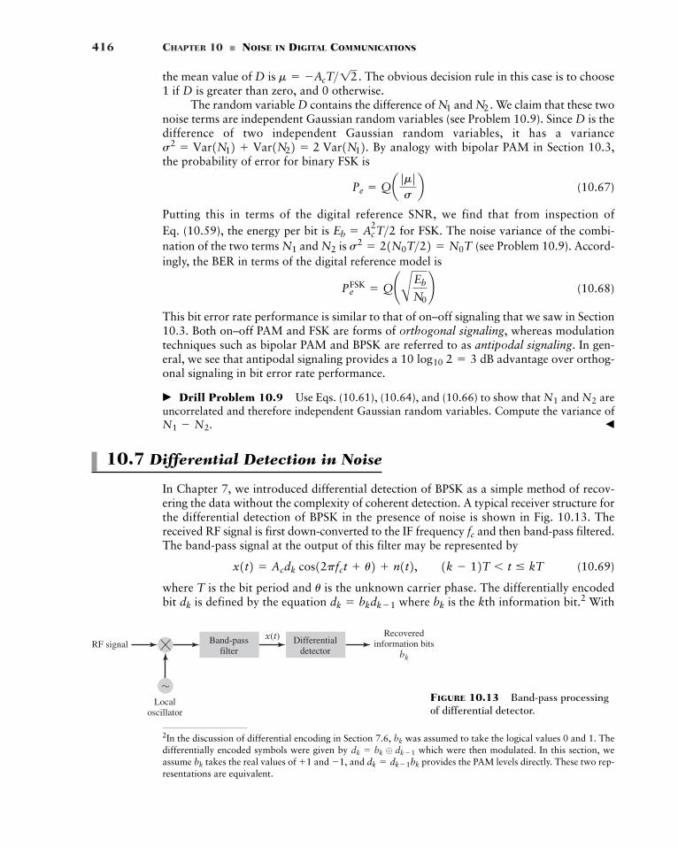
416 CHAPTER 10 � NOISE IN DIGITAL COMMUNICATIONS
the mean value of D is The obvious decision rule in this case is to choose1 if D is greater than zero, and 0 otherwise.
The random variable D contains the difference of and We claim that these twonoise terms are independent Gaussian random variables (see Problem 10.9). Since D is thedifference of two independent Gaussian random variables, it has a variance
By analogy with bipolar PAM in Section 10.3,the probability of error for binary FSK is
(10.67)
Putting this in terms of the digital reference SNR, we find that from inspection of Eq. (10.59), the energy per bit is for FSK. The noise variance of the combi-nation of the two terms and is (see Problem 10.9). Accord-ingly, the BER in terms of the digital reference model is
(10.68)
This bit error rate performance is similar to that of on–off signaling that we saw in Section10.3. Both on–off PAM and FSK are forms of orthogonal signaling, whereas modulationtechniques such as bipolar PAM and BPSK are referred to as antipodal signaling. In gen-eral, we see that antipodal signaling provides a advantage over orthog-onal signaling in bit error rate performance.
� Drill Problem 10.9 Use Eqs. (10.61), (10.64), and (10.66) to show that and areuncorrelated and therefore independent Gaussian random variables. Compute the variance of
�
10.7 Differential Detection in Noise
In Chapter 7, we introduced differential detection of BPSK as a simple method of recov-ering the data without the complexity of coherent detection. A typical receiver structure forthe differential detection of BPSK in the presence of noise is shown in Fig. 10.13. Thereceived RF signal is first down-converted to the IF frequency and then band-pass filtered.The band-pass signal at the output of this filter may be represented by
(10.69)
where T is the bit period and is the unknown carrier phase. The differentially encodedbit is defined by the equation where is the kth information bit.2 Withbkdk � bkdk�1dk
u
x1t2 � Acdk cos12pfct u2 n1t2, 1k � 12T � t � kT
fc
N1 � N2.
N2N1
10 log10 2 � 3 dB
PeFSK � Q¢AEb
N0≤
s2 � 21N0T>22 � N0TN2N1
Eb � Ac2T>2
Pe � Qa ƒm ƒsb
s2 � Var1N12 Var1N22 � 2 Var1N12.N2.N1
m � �AcT>12.
x(t) Recoveredinformation bits
bk
Differentialdetector
Band-passfilter
Localoscillator
RF signal
~FIGURE 10.13 Band-pass processingof differential detector.
2In the discussion of differential encoding in Section 7.6, was assumed to take the logical values 0 and 1. Thedifferentially encoded symbols were given by which were then modulated. In this section, weassume takes the real values of and and provides the PAM levels directly. These two rep-resentations are equivalent.
dk � dk�1bk�1,1bk
dk � bk ⊕ dk�1
bk
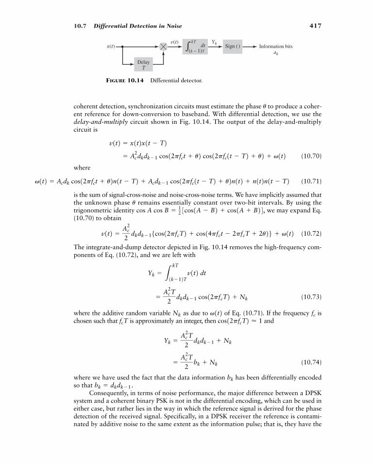
10.7 Differential Detection in Noise 417
Information bitsak
YkdtkT
(k – 1)T�v(t)
x(t)
DelayT
Sign ( )
FIGURE 10.14 Differential detector.
coherent detection, synchronization circuits must estimate the phase to produce a coher-ent reference for down-conversion to baseband. With differential detection, we use thedelay-and-multiply circuit shown in Fig. 10.14. The output of the delay-and-multiplycircuit is
(10.70)
where
(10.71)
is the sum of signal-cross-noise and noise-cross-noise terms. We have implicitly assumed thatthe unknown phase remains essentially constant over two-bit intervals. By using thetrigonometric identity we may expand Eq.(10.70) to obtain
(10.72)
The integrate-and-dump detector depicted in Fig. 10.14 removes the high-frequency com-ponents of Eq. (10.72), and we are left with
(10.73)
where the additive random variable as due to of Eq. (10.71). If the frequency ischosen such that is approximately an integer, then and
(10.74)
where we have used the fact that the data information has been differentially encodedso that
Consequently, in terms of noise performance, the major difference between a DPSKsystem and a coherent binary PSK is not in the differential encoding, which can be used ineither case, but rather lies in the way in which the reference signal is derived for the phasedetection of the received signal. Specifically, in a DPSK receiver the reference is contami-nated by additive noise to the same extent as the information pulse; that is, they have the
bk � dkdk�1.bk
�Ac
2T
2bk Nk
Yk �Ac
2T
2dkdk�1 Nk
cos12pfcT2 � 1fcTfcv1t2Nk
�Ac
2T
2dkdk�1 cos12pfcT2 Nk
Yk � LkT
1k�12T v1t2 dt
v1t2 �Ac
2
2dkdk�15cos12pfcT2 cos14pfct � 2pfcT 2u26 v1t2
cos A cos B � 12 3cos1A � B2 cos1A B24,u
v1t2 � Acdk cos12pfct u2n1t � T2 Acdk�1 cos12pfc1t � T2 u2n1t2 n1t2n1t � T2
� Ac2dkdk�1 cos12pfct u2 cos12pfc1t � T2 u2 v1t2
v1t2 � x1t2x1t � T2
u
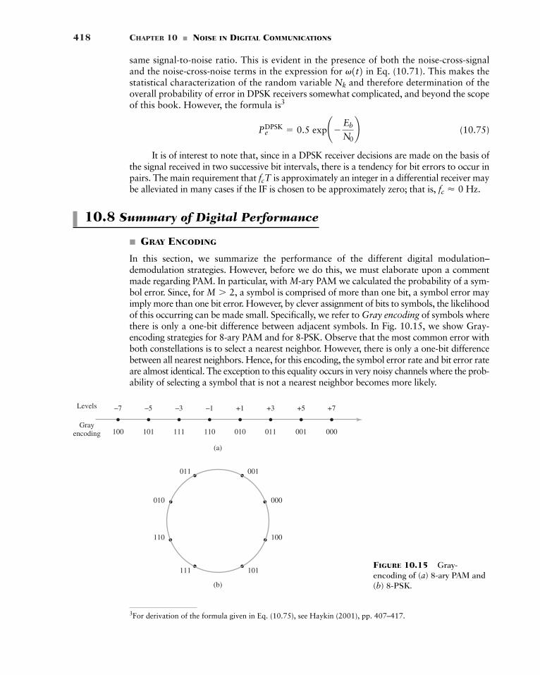
418 CHAPTER 10 � NOISE IN DIGITAL COMMUNICATIONS
same signal-to-noise ratio. This is evident in the presence of both the noise-cross-signaland the noise-cross-noise terms in the expression for in Eq. (10.71). This makes thestatistical characterization of the random variable and therefore determination of theoverall probability of error in DPSK receivers somewhat complicated, and beyond the scopeof this book. However, the formula is3
(10.75)
It is of interest to note that, since in a DPSK receiver decisions are made on the basis ofthe signal received in two successive bit intervals, there is a tendency for bit errors to occur inpairs. The main requirement that is approximately an integer in a differential receiver maybe alleviated in many cases if the IF is chosen to be approximately zero; that is,
10.8 Summary of Digital Performance
� GRAY ENCODING
In this section, we summarize the performance of the different digital modulation–demodulation strategies. However, before we do this, we must elaborate upon a commentmade regarding PAM. In particular, with M-ary PAM we calculated the probability of a sym-bol error. Since, for a symbol is comprised of more than one bit, a symbol error mayimply more than one bit error. However, by clever assignment of bits to symbols, the likelihoodof this occurring can be made small. Specifically, we refer to Gray encoding of symbols wherethere is only a one-bit difference between adjacent symbols. In Fig. 10.15, we show Gray-encoding strategies for 8-ary PAM and for 8-PSK. Observe that the most common error withboth constellations is to select a nearest neighbor. However, there is only a one-bit differencebetween all nearest neighbors. Hence, for this encoding, the symbol error rate and bit error rateare almost identical. The exception to this equality occurs in very noisy channels where the prob-ability of selecting a symbol that is not a nearest neighbor becomes more likely.
M � 2,
fc � 0 Hz.fcT
PeDPSK � 0.5 exp¢�
Eb
N0≤
Nk
v1t2
(a)
(b)
+7
000
+5
001
+3
011
+1
010
–1
110
–3
111
–5
101
–7Levels
Grayencoding 100
011 001
111 101
100
000
110
010
FIGURE 10.15 Gray-encoding of (a) 8-ary PAM and(b) 8-PSK.
3For derivation of the formula given in Eq. (10.75), see Haykin (2001), pp. 407–417.
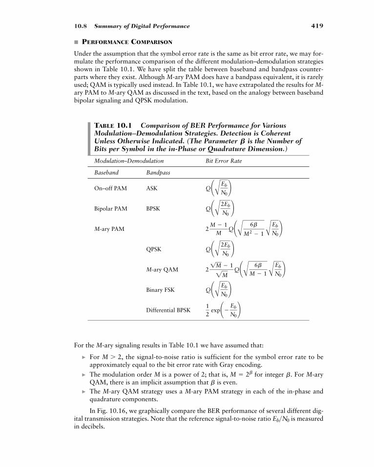
10.8 Summary of Digital Performance 419
� PERFORMANCE COMPARISON
Under the assumption that the symbol error rate is the same as bit error rate, we may for-mulate the performance comparison of the different modulation–demodulation strategiesshown in Table 10.1. We have split the table between baseband and bandpass counter-parts where they exist. Although M-ary PAM does have a bandpass equivalent, it is rarelyused; QAM is typically used instead. In Table 10.1, we have extrapolated the results for M-ary PAM to M-ary QAM as discussed in the text, based on the analogy between basebandbipolar signaling and QPSK modulation.
For the M-ary signaling results in Table 10.1 we have assumed that:
� For the signal-to-noise ratio is sufficient for the symbol error rate to beapproximately equal to the bit error rate with Gray encoding.
� The modulation order M is a power of 2; that is, for integer For M-aryQAM, there is an implicit assumption that is even.
� The M-ary QAM strategy uses a M-ary PAM strategy in each of the in-phase andquadrature components.
In Fig. 10.16, we graphically compare the BER performance of several different dig-ital transmission strategies. Note that the reference signal-to-noise ratio is measuredin decibels.
Eb>N0
b
b.M � 2b
M � 2,
TABLE 10.1 Comparison of BER Performance for VariousModulation–Demodulation Strategies. Detection is CoherentUnless Otherwise Indicated. (The Parameter is the Number ofBits per Symbol in the in-Phase or Quadrature Dimension.)
Modulation–Demodulation Bit Error Rate
Baseband Bandpass
On–off PAM ASK
Bipolar PAM BPSK
M-ary PAM
QPSK
M-ary QAM
Binary FSK
Differential BPSK12
exp¢�Eb
N0≤
Q¢AEb
N0≤
21M � 1
2MQ¢A 6b
M � 1 AEb
N0≤
Q¢A2Eb
N0≤
2M � 1
MQ¢A 6b
M2 � 1 AEb
N0≤
Q¢A2Eb
N0≤
Q¢AEb
N0≤B
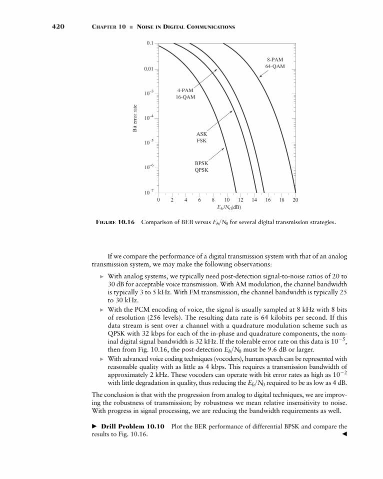
420 CHAPTER 10 � NOISE IN DIGITAL COMMUNICATIONS
Bit
erro
r ra
te
Eb /N0(dB)0 2 4 6 8 10 12 14 16 18 20
10–7
10–6
10–5
10–4
10–3
0.01
0.1
8-PAM64-QAM
4-PAM16-QAM
ASKFSK
BPSKQPSK
FIGURE 10.16 Comparison of BER versus for several digital transmission strategies.Eb>N0
If we compare the performance of a digital transmission system with that of an analogtransmission system, we may make the following observations:
� With analog systems, we typically need post-detection signal-to-noise ratios of 20 to30 dB for acceptable voice transmission. With AM modulation, the channel bandwidthis typically 3 to 5 kHz. With FM transmission, the channel bandwidth is typically 25to 30 kHz.
� With the PCM encoding of voice, the signal is usually sampled at 8 kHz with 8 bitsof resolution (256 levels). The resulting data rate is 64 kilobits per second. If thisdata stream is sent over a channel with a quadrature modulation scheme such asQPSK with 32 kbps for each of the in-phase and quadrature components, the nom-inal digital signal bandwidth is 32 kHz. If the tolerable error rate on this data is then from Fig. 10.16, the post-detection must be 9.6 dB or larger.
� With advanced voice coding techniques (vocoders), human speech can be represented withreasonable quality with as little as 4 kbps. This requires a transmission bandwidth ofapproximately 2 kHz. These vocoders can operate with bit error rates as high as with little degradation in quality, thus reducing the required to be as low as 4 dB.
The conclusion is that with the progression from analog to digital techniques, we are improv-ing the robustness of transmission; by robustness we mean relative insensitivity to noise.With progress in signal processing, we are reducing the bandwidth requirements as well.
� Drill Problem 10.10 Plot the BER performance of differential BPSK and compare theresults to Fig. 10.16. �
Eb>N0
10�2
Eb>N0
10�5,
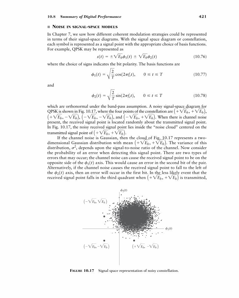
10.8 Summary of Digital Performance 421
� NOISE IN SIGNAL-SPACE MODELS
In Chapter 7, we saw how different coherent modulation strategies could be representedin terms of their signal-space diagrams. With the signal space diagram or constellation,each symbol is represented as a signal point with the appropriate choice of basis functions.For example, QPSK may be represented as
(10.76)
where the choice of signs indicates the bit polarity. The basis functions are
(10.77)
and
(10.78)
which are orthonormal under the band-pass assumption. A noisy signal-space diagram forQPSK is shown in Fig. 10.17, where the four points of the constellation are
and When there is channel noisepresent, the received signal point is located randomly about the transmitted signal point. In Fig. 10.17, the noisy received signal point lies inside the “noise cloud” centered on the transmitted signal point of
If the channel noise is Gaussian, then the cloud of Fig. 10.17 represents a two-dimensional Gaussian distribution with mean The variance of thisdistribution, depends upon the signal-to-noise ratio of the channel. Now considerthe probability of an error when detecting this signal point. There are two types oferrors that may occur; the channel noise can cause the received signal point to be on theopposite side of the axis. This would cause an error in the second bit of the pair.Alternatively, if the channel noise causes the received signal point to fall to the left ofthe axis, then an error will occur in the first bit. In the less likely event that thereceived signal point falls in the third quadrant when is transmitted,A2Eb , 2Eb Bf21t2
f11t2s2,
A2Eb , 2Eb B .A2Eb , 2Eb B .
A�2Eb , 2Eb B .A�2Eb , �2Eb B ,A2Eb , �2Eb B , A2Eb , 2Eb B ,f21t2 � A 2
T sin12pfct2, 0 � t � T
f11t2 � A 2T
cos12pfct2, 0 � t � T
s1t2 � �2Ebf11t2 � 2Ebf21t2
�2(t)
�1(t)
A�3Eb, 3Eb B
A� �3Eb, 3Eb B A �3Eb, 3Eb B
FIGURE 10.17 Signal space representation of noisy constellation.
422 CHAPTER 10 � NOISE IN DIGITAL COMMUNICATIONS
then an error will occur in both bits. Clearly, the probability of either type of error isrelated to the ratio of to the noise standard deviation Although not obvious fromthe diagram, the probability of either type of error is independent of the other.
For this constellation, there is a circle of radius around each signal point in whichno error can occur. That is, is the maximum error distance over which we can alwaysguarantee perfect detection. This signal space can be easily extended to multiple dimensions.For example, if the signal points are then around each signal point,there is a sphere of radius in which noise is guaranteed not to cause an error.
How would we generate such higher dimensional signals in practice? Consider thesignal
where and are as defined in Eqs. (10.77) and (10.78) but extended such they arezero on the interval The remaining two orthonormal functions are given by
(10.79)
and
(10.80)
Under the band-pass assumption, the functions and are clearly orthogonal witheach other and, since they are zero whenever and are nonzero, they are alsoorthogonal to these functions. The resulting signal point is defined by the four-dimensionalvector where is While this four-dimensional space may seem tohave a somewhat artificial construction, its usefulness will become more evident once wediscuss error-correcting codes in the next section.
10.9 Error Detection and Correction
A fundamental characteristic of communication systems is that the receiver has no priorknowledge of the information that is being transmitted across the channel. Consequently,in a digital transmission scheme, when the channel produces errors in the detected bits, itdegrades the quality of communications. In this section, we look at some elementary waysof detecting and correcting errors that occur in transmission.4
In previous sections, we have shown that bit error rate performance of a digital sys-tem depends on the post-detection SNR. If the only channel impairment is additive whiteGaussian noise, then this BER often has an exponential dependence on the SNR, as exem-plified by the Q-function. As a result, the BER quickly becomes very small as the SNRimproves—usually providing much better transmission quality than can be achieved by
�2Eb .si1s1, s2, s3, s42f21t2f11t2 f41t2f31t2
f41t2 � c 0, 0 � t � T
A 2T
sin12pfct2, T � t � 2T
f31t2 � c 0, 0 � t � T
A 2T
cos12pfct2, T � t � 2T
T � t � 2T.f21t2f11t2
s1t2 � s1f11t2 s2f21t2 s3f31t2 s4f41t2
2Eb
A�2Eb , �2Eb , �2Eb B ,2Eb
2Eb
s.2Eb
4The field of error correction and detection was essentially born in the late 1940s with the classic papers of R.Hamming and C. Shannon. Since then an enormous amount of research has been performed in this area. Someintroductory books in the field include Clark and Cain (1981), Lin and Costello (2004) and Blahut (1983). Thematerial in this section is adapted from Arazi (1988).
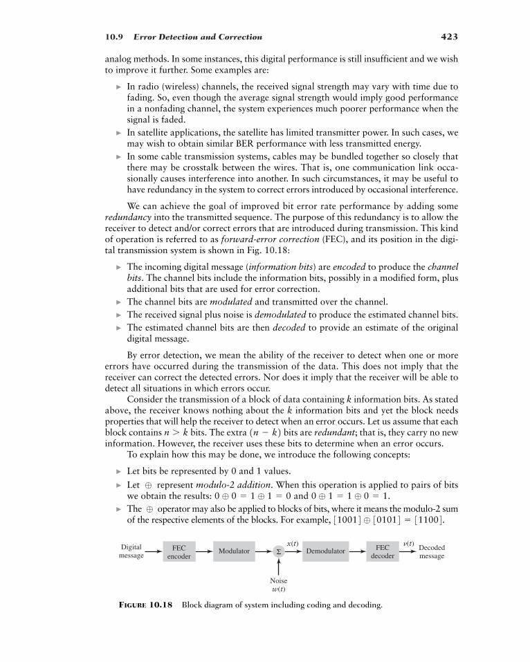
10.9 Error Detection and Correction 423
analog methods. In some instances, this digital performance is still insufficient and we wishto improve it further. Some examples are:
� In radio (wireless) channels, the received signal strength may vary with time due tofading. So, even though the average signal strength would imply good performancein a nonfading channel, the system experiences much poorer performance when thesignal is faded.
� In satellite applications, the satellite has limited transmitter power. In such cases, wemay wish to obtain similar BER performance with less transmitted energy.
� In some cable transmission systems, cables may be bundled together so closely thatthere may be crosstalk between the wires. That is, one communication link occa-sionally causes interference into another. In such circumstances, it may be useful tohave redundancy in the system to correct errors introduced by occasional interference.
We can achieve the goal of improved bit error rate performance by adding someredundancy into the transmitted sequence. The purpose of this redundancy is to allow thereceiver to detect and/or correct errors that are introduced during transmission. This kindof operation is referred to as forward-error correction (FEC), and its position in the digi-tal transmission system is shown in Fig. 10.18:
� The incoming digital message (information bits) are encoded to produce the channelbits. The channel bits include the information bits, possibly in a modified form, plusadditional bits that are used for error correction.
� The channel bits are modulated and transmitted over the channel.� The received signal plus noise is demodulated to produce the estimated channel bits.� The estimated channel bits are then decoded to provide an estimate of the original
digital message.
By error detection, we mean the ability of the receiver to detect when one or moreerrors have occurred during the transmission of the data. This does not imply that thereceiver can correct the detected errors. Nor does it imply that the receiver will be able todetect all situations in which errors occur.
Consider the transmission of a block of data containing k information bits. As statedabove, the receiver knows nothing about the k information bits and yet the block needsproperties that will help the receiver to detect when an error occurs. Let us assume that eachblock contains bits. The extra bits are redundant; that is, they carry no newinformation. However, the receiver uses these bits to determine when an error occurs.
To explain how this may be done, we introduce the following concepts:
� Let bits be represented by 0 and 1 values.
� Let represent modulo-2 addition. When this operation is applied to pairs of bitswe obtain the results: and
� The operator may also be applied to blocks of bits, where it means the modulo-2 sumof the respective elements of the blocks. For example, 310014 ⊕ 301014 � 311004.⊕
0 ⊕ 1 � 1 ⊕ 0 � 1.0 ⊕ 0 � 1 ⊕ 1 � 0⊕
1n � k2n � k
Σ�(t)x(t)
FECencoder
Modulator Demodulator FECdecoder
Decodedmessage
Noisew(t)
Digitalmessage
FIGURE 10.18 Block diagram of system including coding and decoding.
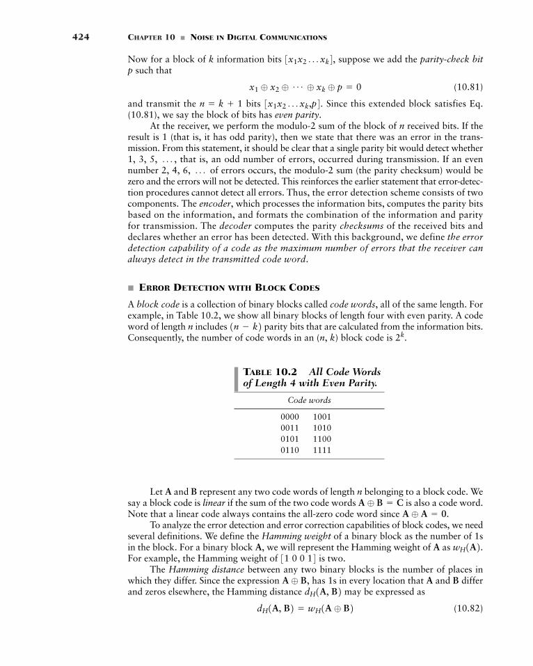
424 CHAPTER 10 � NOISE IN DIGITAL COMMUNICATIONS
Now for a block of k information bits suppose we add the parity-check bitp such that
(10.81)
and transmit the bits Since this extended block satisfies Eq.(10.81), we say the block of bits has even parity.
At the receiver, we perform the modulo-2 sum of the block of n received bits. If theresult is 1 (that is, it has odd parity), then we state that there was an error in the trans-mission. From this statement, it should be clear that a single parity bit would detect whether1, 3, 5, that is, an odd number of errors, occurred during transmission. If an evennumber 2, 4, 6, of errors occurs, the modulo-2 sum (the parity checksum) would bezero and the errors will not be detected. This reinforces the earlier statement that error-detec-tion procedures cannot detect all errors. Thus, the error detection scheme consists of twocomponents. The encoder, which processes the information bits, computes the parity bitsbased on the information, and formats the combination of the information and parityfor transmission. The decoder computes the parity checksums of the received bits anddeclares whether an error has been detected. With this background, we define the errordetection capability of a code as the maximum number of errors that the receiver canalways detect in the transmitted code word.
� ERROR DETECTION WITH BLOCK CODES
A block code is a collection of binary blocks called code words, all of the same length. Forexample, in Table 10.2, we show all binary blocks of length four with even parity. A codeword of length n includes parity bits that are calculated from the information bits.Consequently, the number of code words in an (n, k) block code is 2k.
1n � k2
ÁÁ ,
3x1x2 Á xk,p4.n � k 1
x1 ⊕ x2 ⊕ Á ⊕ xk ⊕ p � 0
3x1x2 Á xk4,
Let A and B represent any two code words of length n belonging to a block code. Wesay a block code is linear if the sum of the two code words is also a code word.Note that a linear code always contains the all-zero code word since
To analyze the error detection and error correction capabilities of block codes, we needseveral definitions. We define the Hamming weight of a binary block as the number of 1sin the block. For a binary block A, we will represent the Hamming weight of A asFor example, the Hamming weight of is two.
The Hamming distance between any two binary blocks is the number of places inwhich they differ. Since the expression has 1s in every location that A and B differand zeros elsewhere, the Hamming distance may be expressed as
(10.82)dH1A, B2 � wH1A ⊕ B2dH1A, B2A ⊕ B,
31 0 0 14 wH1A2.A ⊕ A � 0.
A ⊕ B � C
TABLE 10.2 All Code Wordsof Length 4 with Even Parity.
Code words
0000 10010011 10100101 11000110 1111
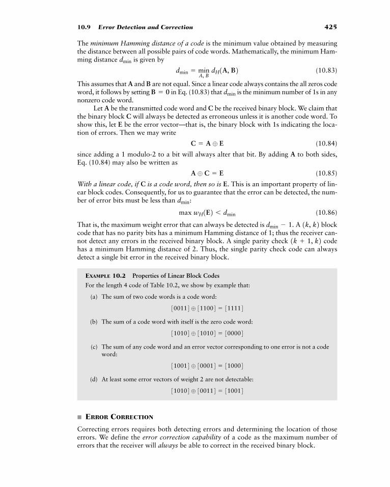
10.9 Error Detection and Correction 425
The minimum Hamming distance of a code is the minimum value obtained by measuringthe distance between all possible pairs of code words. Mathematically, the minimum Ham-ming distance is given by
(10.83)
This assumes that A and B are not equal. Since a linear code always contains the all zeros codeword, it follows by setting in Eq. (10.83) that is the minimum number of 1s in anynonzero code word.
Let A be the transmitted code word and C be the received binary block. We claim thatthe binary block C will always be detected as erroneous unless it is another code word. Toshow this, let E be the error vector—that is, the binary block with 1s indicating the loca-tion of errors. Then we may write
(10.84)
since adding a 1 modulo-2 to a bit will always alter that bit. By adding A to both sides, Eq. (10.84) may also be written as
(10.85)
With a linear code, if C is a code word, then so is E. This is an important property of lin-ear block codes. Consequently, for us to guarantee that the error can be detected, the num-ber of error bits must be less than
(10.86)
That is, the maximum weight error that can always be detected is A blockcode that has no parity bits has a minimum Hamming distance of 1; thus the receiver can-not detect any errors in the received binary block. A single parity check codehas a minimum Hamming distance of 2. Thus, the single parity check code can alwaysdetect a single bit error in the received binary block.
EXAMPLE 10.2 Properties of Linear Block Codes
For the length 4 code of Table 10.2, we show by example that:
(a) The sum of two code words is a code word:
(b) The sum of a code word with itself is the zero code word:
(c) The sum of any code word and an error vector corresponding to one error is not a codeword:
(d) At least some error vectors of weight 2 are not detectable:
� ERROR CORRECTION
Correcting errors requires both detecting errors and determining the location of thoseerrors. We define the error correction capability of a code as the maximum number oferrors that the receiver will always be able to correct in the received binary block.
310104 ⊕ 300114 � 310014
310014 ⊕ 300014 � 310004
310104 ⊕ 310104 � 300004
300114 ⊕ 311004 � 311114
1k 1, k21k, k2dmin � 1.
max wH1E2 � dmin
dmin:
A ⊕ C � E
C � A ⊕ E
dminB � 0
dmin � minA, B
dH1A, B2dmin
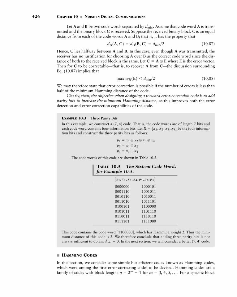
426 CHAPTER 10 � NOISE IN DIGITAL COMMUNICATIONS
Let A and B be two code words separated by Assume that code word A is trans-mitted and the binary block C is received. Suppose the received binary block C is an equaldistance from each of the code words A and B; that is, it has the property that
(10.87)
Hence, C lies halfway between A and B. In this case, even though A was transmitted, thereceiver has no justification for choosing A over B as the correct code word since the dis-tance of both to the received block is the same. Let where E is the error vector.Then for C to be correctable—that is, to recover A from C—the discussion surroundingEq. (10.87) implies that
(10.88)
We may therefore state that error correction is possible if the number of errors is less thanhalf of the minimum Hamming distance of the code.
Clearly, then, the objective when designing a forward error-correction code is to addparity bits to increase the minimum Hamming distance, as this improves both the errordetection and error-correction capabilities of the code.
EXAMPLE 10.3 Three Parity Bits
In this example, we construct a (7, 4) code. That is, the code words are of length 7 bits andeach code word contains four information bits. Let be the four informa-tion bits and construct the three parity bits as follows:
The code words of this code are shown in Table 10.3.
p3 � x3 ⊕ x4
p2 � x1 ⊕ x2
p1 � x1 ⊕ x2 ⊕ x3 ⊕ x4
X � 3x1, x2, x3, x44
max wH1E2 � dmin>2
C � A ⊕ E
dH1A, C2 � dH1B, C2 � dmin>2
dmin.
TABLE 10.3 The Sixteen Code Wordsfor Example 10.3.
0000000 10001010001110 10010110010110 10100110011010 10111010100101 11000000101011 11011100110011 11101100111101 1111000
3x1, x2, x3, x4, p1, p2, p34
This code contains the code word which has Hamming weight 2. Thus the mini-mum distance of this code is 2. We therefore conclude that adding three parity bits is notalways sufficient to obtain In the next section, we will consider a better (7, 4) code.
� HAMMING CODES
In this section, we consider some simple but efficient codes known as Hamming codes,which were among the first error-correcting codes to be devised. Hamming codes are afamily of codes with block lengths for For a specific blockm � 3, 4, 5, Á .n � 2m � 1
dmin � 3.
311000004,
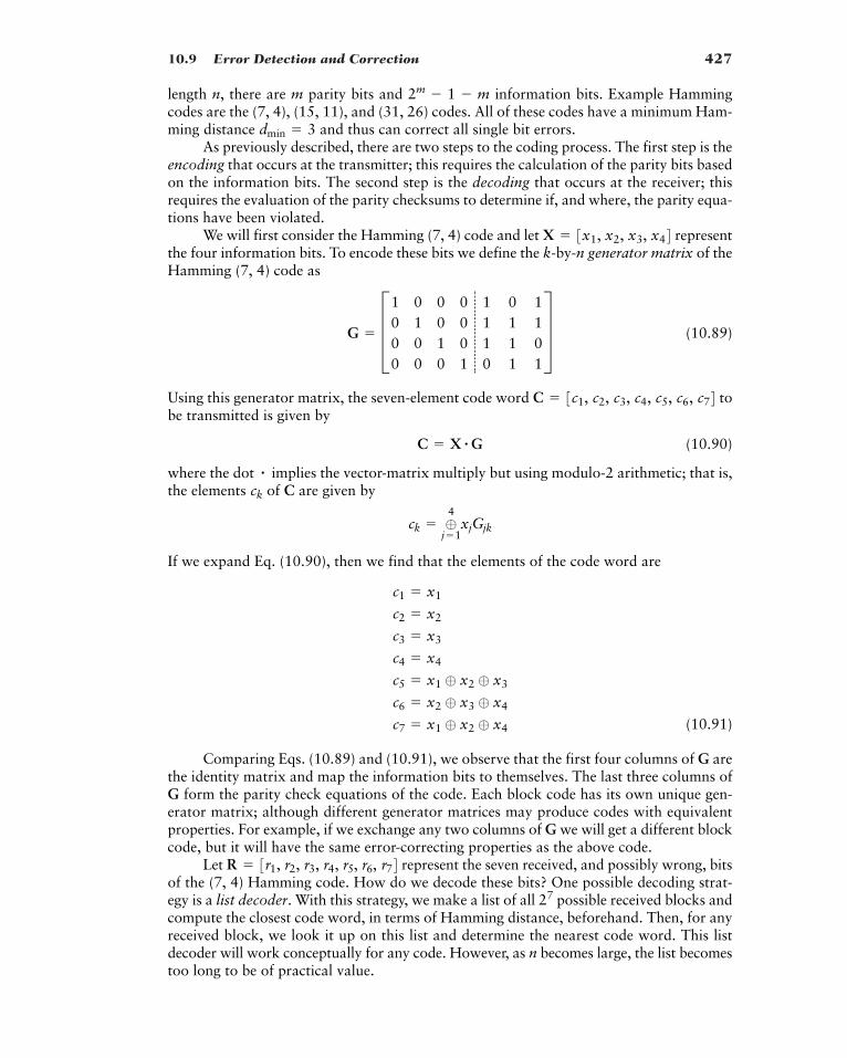
10.9 Error Detection and Correction 427
length n, there are m parity bits and information bits. Example Hammingcodes are the (7, 4), (15, 11), and (31, 26) codes. All of these codes have a minimum Ham-ming distance and thus can correct all single bit errors.
As previously described, there are two steps to the coding process. The first step is theencoding that occurs at the transmitter; this requires the calculation of the parity bits basedon the information bits. The second step is the decoding that occurs at the receiver; thisrequires the evaluation of the parity checksums to determine if, and where, the parity equa-tions have been violated.
We will first consider the Hamming (7, 4) code and let representthe four information bits. To encode these bits we define the k-by-n generator matrix of theHamming (7, 4) code as
(10.89)
Using this generator matrix, the seven-element code word tobe transmitted is given by
(10.90)
where the dot implies the vector-matrix multiply but using modulo-2 arithmetic; that is,the elements of C are given by
If we expand Eq. (10.90), then we find that the elements of the code word are
(10.91)
Comparing Eqs. (10.89) and (10.91), we observe that the first four columns of G arethe identity matrix and map the information bits to themselves. The last three columns ofG form the parity check equations of the code. Each block code has its own unique gen-erator matrix; although different generator matrices may produce codes with equivalentproperties. For example, if we exchange any two columns of G we will get a different blockcode, but it will have the same error-correcting properties as the above code.
Let represent the seven received, and possibly wrong, bitsof the (7, 4) Hamming code. How do we decode these bits? One possible decoding strat-egy is a list decoder. With this strategy, we make a list of all possible received blocks andcompute the closest code word, in terms of Hamming distance, beforehand. Then, for anyreceived block, we look it up on this list and determine the nearest code word. This listdecoder will work conceptually for any code. However, as n becomes large, the list becomestoo long to be of practical value.
27
R � 3r1, r2, r3, r4, r5, r6, r74
c7 � x1 ⊕ x2 ⊕ x4
c6 � x2 ⊕ x3 ⊕ x4
c5 � x1 ⊕ x2 ⊕ x3
c4 � x4
c3 � x3
c2 � x2
c1 � x1
ck � ⊕4
j�1xjGjk
ck
#C � X # G
C � 3c1, c2, c3, c4, c5, c6, c74
G � D1 0 0 00 1 0 00 0 1 00 0 0 1
1 0 11 1 11 1 00 1 1
TX � 3x1, x2, x3, x44
dmin � 3
2m � 1 � m
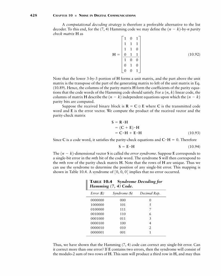
428 CHAPTER 10 � NOISE IN DIGITAL COMMUNICATIONS
A computational decoding strategy is therefore a preferable alternative to the listdecoder. To this end, for the (7, 4) Hamming code we may define the paritycheck matrix H as
(10.92)
Note that the lower 3-by-3 portion of H forms a unit matrix, and the part above the unitmatrix is the transpose of the part of the generating matrix to left of the unit matrix in Eq.(10.89). Hence, the columns of the parity matrix H form the coefficients of the parity equa-tions that the code words of the Hamming code should satisfy. For a linear code, thecolumns of matrix H describe the independent equations upon which the parity bits are computed.
Suppose the received binary block is where C is the transmitted codeword and E is the error vector. We compute the product of the received vector and theparity-check matrix
(10.93)
Since C is a code word, it satisfies the parity-check equations and Therefore
(10.94)
The -dimensional vector S is called the error syndrome. Suppose E corresponds toa single-bit error in the mth bit of the code word. The syndrome S will then correspond tothe mth row of the parity check matrix H. Note that the rows of H are unique. Thus wecan use the syndrome to determine the position of any single-bit error. This mapping isshown in Table 10.4. A syndrome of implies that no error occurred.30, 0, 04
1n � k2S � E # H
C # H � 0.
� C # H E # H� 1C E2 # HS � R # H
R � C ⊕ E
1n � k21n � k2 1n, k2
H � G1 0 11 1 11 1 00 1 11 0 00 1 00 0 1
W1n � k2-by-n
TABLE 10.4 Syndrome Decoding forHamming (7, 4) Code.
Error (E) Syndrome (S) Decimal Rep.
0000000 000 01000000 101 50100000 111 70010000 110 60001000 011 30000100 100 40000010 010 20000001 001 1
Thus, we have shown that the Hamming (7, 4) code can correct any single-bit error. Canit correct more than one error? If E contains two errors, then the syndrome will consist ofthe modulo-2 sum of two rows of H. This sum will produce a third row in H, and may thus
10.9 Error Detection and Correction 429
be indistinguishable from the single-bit error that also produces this row. Consequently, theHamming (7, 4) code can correct all single-bit errors but not two-bit errors. In other words,the of the code must be 3.
On the error-detection side, we again note that any two-bit error will produce a thirdrow of H. Since this third row is nonzero, this means we can detect (but not correct) all two-bit errors with the Hamming (7, 4) code. Note, however, that if the three-bit error
occurs, then the syndrome Therefore, the code cannot detect allthree-bit errors. This provides further confirmation that is 3 for this code.
EXAMPLE 10.4 Error Correction with a Hamming Code
Four information bits are encoded with a Hamming (7, 4) code whose generator matrix isgiven by Eq. (10.89). The received bit sequence is What sequence was trans-mitted if one error occurred during the transmission?
Multiplying R by the parity check matrix, we obtain the error syndrome
Since the error syndrome is nonzero, we know that one or more errors occurred. From Table10.4, a single error in the second bit from the left would cause this sequence, so we concludethat the transmitted sequence is and the information bits are
EXAMPLE 10.5 Probability of Block Error
Suppose a BPSK transmission strategy is encoded with a (7, 4) Hamming block code. Comparethe block error rate with and without decoding.
From Section 10.4 the probability of a bit error with BPSK is Ablock of uncoded seven bits is received correctly if it contains no errors. The probability of ablock error—that is, one or more bit errors—is the complement of this; namely,
(10.95)
With the (7, 4) Hamming code, the probability of a block error is the probability of two or moreerrors over a seven-bit block. This probability is given by
(10.96)
where is the probability of a bit error with a Hamming code. If , then the probabilityof a block error is clearly reduced with the Hamming code. However, there is a nuance thatmust be considered. This is why we have used in the Eq. (10.96) as opposed to In par-ticular, in the digital reference model, refers to the energy per information bit. With theHamming (7, 4) code, we are transmitting four information bits and three parity bits, for a totalof seven channel bits per block. Letting represent the energy per channel bit, we find thatthe energy of seven channel bits corresponds to the energy of four information bits:
(10.97)
Furthermore, the probability of error in Eq. (10.96) represents the probability of a channel-bit error, so using the probability of error for BPSK and Eq. (10.97), we have
(10.98)� Q¢A 8Eb
7N0≤
Peœ � Q¢A2Ec
N0≤
Peœ
Ec �47
Eb
Ec
Eb
Pe .Peœ
Peœ � PePe
œ
Pbcoded
� 1 � 11 � Peœ27 � a7
1b11 � Pe
œ26Peœ
Pbuncoded
� 1 � 11 � Pe27
Pe � Q A22Eb>N0 B .
310014.310011104
� 31114S � R # H
R � 311011104.
dmin
S � 0.E � 310110004
dmin
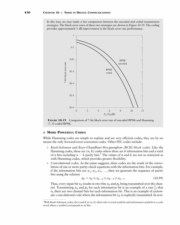
430 CHAPTER 10 � NOISE IN DIGITAL COMMUNICATIONS
5With Reed–Solomon codes, the n and k in often refer to total symbols and information symbols in a codeword where a symbol corresponds to m bits.
1n, k2
In this way, we may make a fair comparison between the uncoded and coded transmissionstrategies. The block error rates of these two strategies are shown in Figure 10.19. The codingprovides approximately 1 dB improvement in the block error rate performance.
7-bi
t blo
ck e
rror
rat
e
Eb /N0(dB)0 2 4 6 8 10 12
1E-6
1
0.1
0.01
1E-3
1E-4
1E-5
BPSKcoded
BPSKuncoded
FIGURE 10.19 Comparison of 7-bit block error rate of uncoded BPSK and Hamming(7, 4) coded BPSK.
� MORE POWERFUL CODES
While Hamming codes are simple to explain and are very efficient codes, they are by nomeans the only forward-error-correction codes. Other FEC codes include:
� Reed–Solomon and Bose–Chaudhuri–Hocquenghem (BCH) block codes. Like theHamming codes, these are codes where there are k information bits and a totalof n bits including parity bits.5 The values of n and k are not as restricted aswith Hamming codes, which provides greater flexibility.
� Convolutional codes. As the name suggests, these codes are the result of the convo-lution of one or more parity-check equations with the information bits. For example,if the information bits are then we generate the sequence of paritybits using the relation
(10.99)
Thus, every input bit results in two bits and being transmitted over the chan-nel. Transmitting and for each information bit is an example of a rate thatis, there are two channel bits for each information bit. This is an example of system-atic convolutional code where the information bit is explicitly transmitted. In non-xk
12 ;pkxk
pkxkxk
pk � xk ⊕ xk�2 ⊕ xk�3 ⊕ xk�5
x1, x2, x3, Á ,
n � k1n, k2
10.9 Error Detection and Correction 431
systematic convolutional codes there may be two parity equations such as Eq. (10.99),and the two parity bits produced for each information bit are transmitted but theinformation bit is not. The error-correcting capabilities of a convolutional code areusually determined by the span (in bits) of the parity-check equation, which is referredto as the memory of the code. Unfortunately, the decoding complexity increases expo-nentially with the memory of the code, so practical codes are usually limited to mem-ory of less than ten bits.
� Turbo codes. Turbo codes are block codes but use a continuous encoding strategy sim-ilar to convolutional codes. For example, with a rate Turbo code, the three trans-mitted bits for each information bit could be
(10.100)
With Turbo codes, the parity is determined by a recursive equation; that is, the kth par-ity bit depends upon the parity bit as well as the input bits. Note that in Eq.(10.100) the formula for the p and q parity bits are the same; the difference is that theq-formula uses which refers to the same information bits but in an interleavedorder. Interleaving means shuffling the order of the bits in a pseudo-random fashion.
For both block codes and convolutional codes, the general principle is to add paritybits in such a way as to maximize the minimum distance However, maximizing theminimum distance is subject to two important constraints:
1. The code rate; that is, the ratio of the number of information bits to the total num-ber of bits in a code word must be reasonable. This ensures that the communicationsystem has a significant information throughput.
2. The code must permit a practical decoding strategy. It is relatively easy to constructcodes with large minimum distances, but the corresponding decoding strategies areoften too complex to be of practical use.
Even with practical decoding strategies and large minimum distances, there are lim-its to how reliable data can be transmitted. The theoretical limits fall in the area of Shan-non channel capacity theory. Shannon theory6 tells us that if the transmission rate is belowthe channel capacity, then there exist forward error-correcting codes that permit error-freetransmission. Enormous strides in approaching these theoretical limits have been made inrecent years with the discovery of Turbo codes. Turbo codes draw features from both con-volutional and block codes. Although is important in the design of Turbo codes, otherdistinct features of these codes improve performance at low signal-to-noise ratios.
� SIGNAL-SPACE INTERPRETATION OF FORWARD-ERROR-CORRECTION CODES
In Section 10.8 we saw how we could construct a four-dimensional vector with a signal-space representation of
(10.101)
where there are sixteen points in the constellation defined by s. To be specific, we considerthe construction of an N-dimensional signal vector in the context of error-correcting codes.
For a linear code, we defined a code word c of length N comprised of informa-
� 2Eb3�1, �1, �1, �14s � C�2Eb , �2Eb , �2Eb , �2Eb D
dmin
dmin.
xki ,
1k � 12thqk � qk�1 ⊕ xk
i ⊕ xk�2i ⊕ xk�4
i
pk � pk�1 ⊕ xk ⊕ xk�2 ⊕ xk�4
xk
xk
13
xk
xk
6For a discussion of the Shannon theory and its implications, see the book by Cover and Thomas (1991).
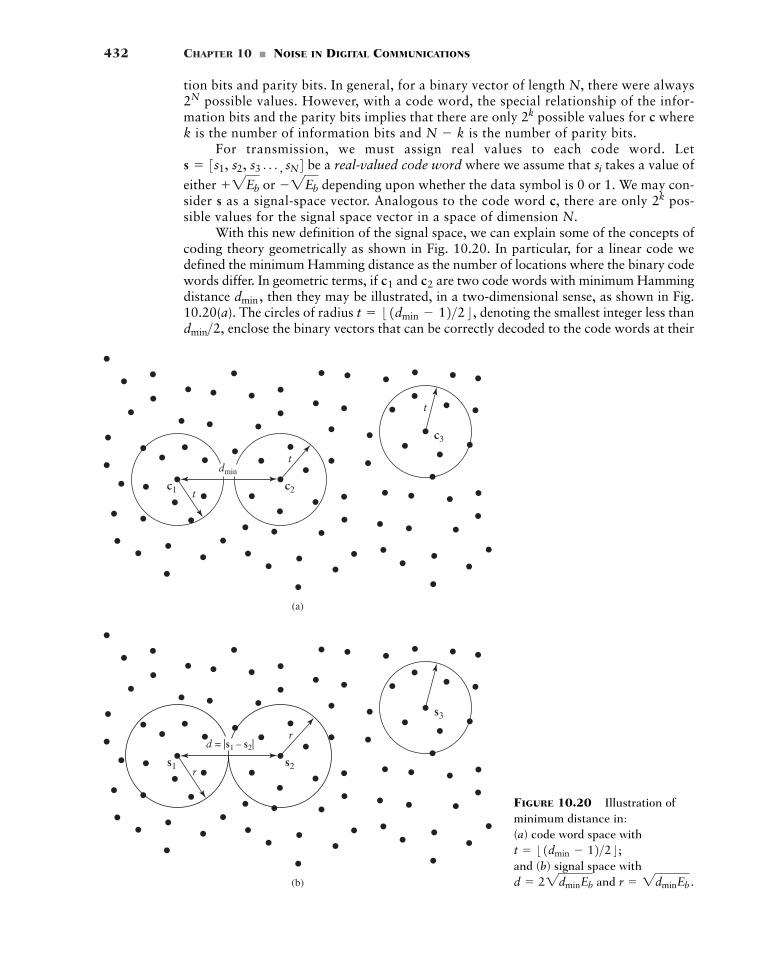
432 CHAPTER 10 � NOISE IN DIGITAL COMMUNICATIONS
(a)
(b)
s3
s1r
r
s2
d = |s1 – s2|
c3
c1 c2
dmin
t
t
t
FIGURE 10.20 Illustration ofminimum distance in: (a) code word space with
and (b) signal space withand r � 2dminEb .d � 22dminEb
t � :1dmin � 12>2; ;
tion bits and parity bits. In general, for a binary vector of length N, there were alwayspossible values. However, with a code word, the special relationship of the infor-
mation bits and the parity bits implies that there are only possible values for c wherek is the number of information bits and is the number of parity bits.
For transmission, we must assign real values to each code word. Letbe a real-valued code word where we assume that takes a value of
either or depending upon whether the data symbol is 0 or 1. We may con-sider s as a signal-space vector. Analogous to the code word c, there are only pos-sible values for the signal space vector in a space of dimension N.
With this new definition of the signal space, we can explain some of the concepts ofcoding theory geometrically as shown in Fig. 10.20. In particular, for a linear code wedefined the minimum Hamming distance as the number of locations where the binary codewords differ. In geometric terms, if and are two code words with minimum Hammingdistance then they may be illustrated, in a two-dimensional sense, as shown in Fig.10.20(a). The circles of radius denoting the smallest integer less than
enclose the binary vectors that can be correctly decoded to the code words at theirdmin>2,t � :1dmin � 12>2; ,dmin,
c2c1
2k�2Eb2Eb
sis � 3s1, s2, s3 Á , sN4N � k
2k2N
10.10 Summary and Discussion 433
respective centers. In reality, these circles represent N-dimensional spheres.In signal space, the squared geometric (Euclidean) distance between two neighboring
signal space vectors is defined by the squared Euclidean distance
(10.102)
where we have used the fact that neighboring signal-space vectors, and differ in ele-ments if they represent code words. Thus, the Hamming distance between code words and thegeometric distance between their corresponding signal-space vectors are directly related. Incode space, we may select two code words of minimum separation and draw spheres of radiust around them. Since the code has minimum distance this implies there are no other codewords within this sphere; any point within this sphere will be closer to its center than to any othercode word. Similarly, in signal space, we may draw spheres of radius aroundeach signal space vector representing a code word, as shown in Fig. 10.20(b), and there are noother signal space vectors representing code words within this sphere.
This resonates with our definition of the error correction capability of a code: Anyreceived signal that lies within a distance of the transmitted code can be uniquely cor-rected to that code word. Received signals that are beyond this distance may be erroneouslycorrected if they fall in other spheres or they may be properly corrected if they fall in the gapsbetween spheres and are closer to the transmitted code word than any other. The error detec-tion capability means the received signal does not fall directly on another code word.
The Hamming (7, 4) code is an example that has code word (points) in a seven-dimensional signal space and the minimum distance between any two code words is three.Similarly, the Hamming (15, 11) codes is an example that has code words (points) ina 15-dimensional space and again the minimum distance is three.
10.10 Summary and Discussion
In this chapter, we investigated the detection of digitally modulated signals in noise. Webegan by establishing bit error rate (BER) as the figure of merit for comparing digital com-munication systems and observed that BER is typically not a linear function of the signal-to-noise ratio. Next, we addressed the detection of various digital modulation schemes inthe presence of noise and made the following observations:
(i) Analysis of the detection of a single pulse in noise shows the optimality of matchedfiltering. The matched-filter principle is a mainstay for the subsequent digital detec-tion techniques. We showed that the bit error rate performance using matched filteringwas closely related to the Q-function that was defined in Chapter 8.
(ii) We showed how the principle of matched filtering may be extended to the detectionof pulse-amplitude modulation, and that bit error rate performance may be deter-mined in a manner similar to single-pulse detection.
(iii) We discussed how the receiver structure for the coherent detection of band-pass mod-ulation strategies such as BPSK, QPSK, and QAM was similar to coherent detectionof corresponding analog signals. After down-conversion to baseband, the principle ofmatched filtering also applies to these modulation strategies, and BER performanceequivalent to the corresponding baseband systems is thereby obtained.
211
24
dmin>2
r � 2dminEb
dmin,
dmins2,s1
� 4dminEb
� dmin A22Eb B2� a
N
i�11s1i � s2i22
d2 � ‘ s1 � s2 ‘ 2
434 CHAPTER 10 � NOISE IN DIGITAL COMMUNICATIONS
(iv) We showed how quadrature modulation schemes such as QPSK and QAM providethe same performance as their one-dimensional counterparts of BPSK and PAM, dueto the orthogonality of the in-phase and quadrature components of the modulated sig-nals. In particular, we showed how QPSK modulation provides the same BER asBPSK for the same but provides double the throughput.
(v) We also showed that antipodal strategies such as BPSK are more power efficient thanorthogonal transmission strategies such as on–off signaling and FSK.
(vi) We introduced the concept of non-coherent detection when we illustrated that BPSK couldbe detected using a new approach where the transmitted bits are differentially encoded.The simplicity of this detection technique results in a small BER performance penalty.
The signal-space concepts introduced in Chapter 7 provide an intuitive geometrical inter-pretation of the relative performance of the different coherent digital modulation strategiesin noise. Finally, we closed the chapter with a brief introduction of forward error correc-tion coding, which can be combined with any of the above digital modulation strategies toreduce the power required to achieve the same bit error rate performance—however, thereis usually a power and bandwidth tradeoff that must be made when using forward-error-correction coding in the design of digital communication systems.
ADDITIONAL PROBLEMS
10.11 A communications system that transmits single isolated pulses is subject to multipath such that,if the transmitted pulse is of lenght T, the received signal is
Assuming that and are known, determine the optimum receiver filter for signal in the pres-ence of white Gaussian noise of power spectral density . What is the post-detection SNRat the output of this filter?
10.12 The impulse response corresponding to a root-raised cosine spectrum, normalized to satisfy Eq.(10.10), is given by
where is the symbol period and is the roll-off factor. Obtain a discrete-time rep-resentation of this impulse response by sampling it at for integer n such that
Numerically approximate matched filtering (e.g. with MatLab) by performingthe discrete-time convolution
where What is the value of and 0?10.13 Determine the discrete-time autocorrelation function of the noise sequence defined by Eq. (10.34)
where w(t) is a white Gaussian noise process and the pulse p(t) corresponds to a root-raised cosinespectrum. How are the noise samples corresponding to adjacent bit intervals related?
10.14 Draw the Gray-encoded constellation (signal-space diagram) for 16-QAM and for 64-QAM. Canyou suggest a constellation for 32-QAM?
Nk � L�
� �p(kT � t)w(t)dt
{Nk}qk � q(0.1kT) for k � �20, �10,gn � g(0.1nT).
a60
n� �60gngk�nqk � 0.1
�3T � t � 3T.t � 0.1nT
aT � 1>(2B0)
g(t) � ¢4ap≤ cosB (1 a)pt
TR
T4at
sinB (1 � a)ptT
R1 � ¢4at
T≤2
N0>2ta
s1t2 � p1t2 ap1t � t2p1t2
Eb>N0
Advanced Problems 435
10.15 Write the defining equation for a QAM-modulated signal. Based on the discussion of QPSKand multi-level PAM, draw the block diagram for a coherent QAM receiver.
10.16 Show that the if T is a multiple of the period of then the terms and are orthogonal over the interval
10.17 For a rectangular pulse shape, by how much does the null-to-null transmission bandwidthincrease, if the transmission rate is increased by a factor of three?
10.18 Under the bandpass assumptions, determine the conditions under which the two signalsand are orthogonal over the interval from 0 to T.
10.19 Encode the sequence 1101 with a Hamming (7, 4) block code.
10.20 The Hamming (7, 4) encoded sequence 1001000 was received. If the number of transmissionerrors is less than two, what was the transmitted sequence?
10.21 A Hamming (15, 11) block code is applied to a BPSK transmission scheme. Compare the blockerror rate performance of the uncoded and coded systems. Explain how this would differ if themodulation strategy was QPSK.
ADVANCED PROBLEMS
10.22 Show that the choice minimizes the probability of error given by Eq. (10.26). Hint: The Q-function is continuously differentiable.
10.23 For M-ary PAM,
(a) Show that the formula for probability of error, namely,
holds for 3, and 4. By mathematical induction, show that it holds for all M.
(b) Show the formula for average power, namely,
holds for and 3. Show it holds for all M.10.24 Consider binary FSK transmission where is not an integer.
(a) What is the mean output of the upper correlator of Fig. 10.12, if a 1 is transmitted? Whatis the mean output of the lower correlator?
(b) Are the random variables and independent under these conditions? What is the vari-ance of
(c) Describe the properties of the random variable D of Fig. 10.12 in this case.10.25 Show that the noise variance of the in-phase component of the band-pass noise is the same
as the band-pass noise variance; that is, for a band-pass noise of bandwidth , we have
10.26 In this problem, we investigate the effects when transmit and receive filters do not combine toform an ISI-free pulse shape. To be specific, data are transmitted at baseband using binary PAMwith an exponential pulse shape where T is the symbol period (see Exam-ple 2.2). The receiver detects the data using an integrate-and-dump detector.
(a) With data symbols represented as , what is magnitude of the signal component at the out-put of the detector?
(b) What is the worst case magnitude of the intersymbol interference at the output of the detec-tor. (Assume the data stream has infinite length.) Using the value obtained in part (a) as areference, by what percentage is the eye opening reduced by this interference.
�1
g(t) � exp(t>T)u(t)
E3nI21t24 � N0BN
BNn1t2 nI1t2N1 � N2?
N2N1
1f1 � f22TM � 2,
P �(M2 � 1)A2
3
M � 2,
Pe � 2aM � 1M
bQaAsb
g � m>2
cos12pf1t2cos12pf0t2
3t0 , T t04. cos12pfct2sin12pfct2fc ,
436 CHAPTER 10 � NOISE IN DIGITAL COMMUNICATIONS
(c) What is the rms magnitude of the intersymbol interference at the output of the detector? Ifthis interference is treated as equivalent to noise, what is the equivalent signal-to-noise ratioat the output of the detector? Comment on how this would affect bit error rate perfor-mance of this system when there is also receiver noise present.
10.27 A BPSK signal is applied to a matched-filter receiver that lacks perfect phase synchronizationwith the transmitter. Specifically, it is supplied with a local carrier whose phase differs fromthat of the carrier used in the transmitter by radians.
(a) Determine the effect of the phase error on the average probability of error of this receiver.(b) As a check on the formula derived in part (a), show that when the phase error is zero the
formula reduces to the same form as in Eq. (10.44).10.28 A binary FSK system transmits data at the rate of 2.5 times megabits per second. During the
course of transmission, white Gaussian noise of zero mean and power spectral density watts per hertz is added to the signal. In the absence of noise, the amplitude of the received sig-nal is across 50 ohm impedance. Determine the average probability of error assumingcoherent detection of the binary FSK signal.
10.29 One of the simplest forms of forward error correction code is the repetition code. With an N-repetition code, the same bit is sent N times, and the decoder decides in favor of the bit that isdetected on the majority of trials (assuming N is odd). For a BPSK transmission scheme, deter-mine the BER performance of a 3-repetition code.
� COMPUTER EXPERIMENTS
10.30 In this experiment, we simulate the performance of bipolar signaling in additive white Gauss-ian noise. The MATLAB script included in Appendix 7 for this experiment does the following:
• It generates a random sequence with rectangular pulse shaping.• It adds Gaussian noise.• It detects the data with a simulated integrate-and-dump detector.
With this MATLAB script:(a) Compute the spectrum of the transmitted signal and compare to the theoretical.(b) Explain the computation of the noise variance given an ratio.(c) Confirm the theoretically predicted bit error rate for from 0 to 10 dB.
10.31 In this experiment, we simulate the performance of bipolar signaling in additive white Gauss-ian noise but with root-raised-cosine pulse shaping. A MATLAB script is included in Appendix7 for doing this simulation. Hence, do the following:(a) Compute the spectrum of the transmitted signal and compare to the theoretical. Also com-
pare to the transmit spectrum with rectangular pulse shaping.(b) Plot the eye diagram of the received signal under no noise conditions. Explain the relation-
ship of the eye opening to the bit error rate performance.(c) Confirm the theoretically predicted bit error rate for from 0 to 10 dB.
10.32 In this experiment, we simulate the effect of various mismatches in the communication systemand their effects on performance. In particular, modify the MATLAB scripts of the two pre-ceding problems to do the following:(a) Simulate the performance of a system using rectangular pulse-shaping at the transmitter
and raised cosine pulse shaping at the receiver. Comment on the performance degradation.(b) In the case of matched root-raised cosine filtering, include a complex phase rotation
in the channel. Plot the resulting eye diagram for being the equivalent of 5°, 10°, 20°, and45°. compare to the case of 0°. Do likewise for the BER performance. What modifi-cation to the theoretical BER formula would accurately model this behavior?
u �u
exp1ju2
Eb>N0
Eb>N0
Eb>N0
1 mV
10�20
f
f
437
CHAPTER 11
SYSTEM AND NOISE
CALCULATIONS
The inevitable presence of noise undermines the reliable transmission of signals through acommunication system. In previous chapters, we have modeled noise as white, Gaussian,and additive. This model was mathematically tractable and allowed us to obtain numerousanalytical results about the performance of analog and digital communications in noise. Inthose previous chapters, we claimed that white Gaussian model was a reasonable model ofreality. Now we consider in greater detail the potential sources of noise and how theyarise. The sources of noise may be external to the system (e.g., atmospheric noise, galacticnoise, manmade noise) or internal to the system. The second category includes an impor-tant type of noise that arises due to spontaneous fluctuations of current or voltage in elec-trical circuits. This type of noise, in one way or another, is present in every communicationsystem and represents a fundamental limitation on the transmission and detection ofsignals.
In this chapter, we briefly discuss the physical sources of noise in electrical circuitsand develop quantitative models for measuring and predicting the presence of noise in acommunication system. We then consider the effect propagation has on the received powerlevel. In particular, we consider free-space propagation of radio waves and the propagationof radio waves in a terrestrial mobile environment. When the two concepts of received sig-nal level and system noise level are combined, we have the signal-to-noise ratio, which rep-resents the fundamental figure of merit for the quality of transmission across acommunication channel.
This chapter teaches us the following lessons:
� Lesson 1: Noise in communication systems may be generated by a number of sources, butoften the sources are the communication devices themselves. Thermal noise and shot noiseare examples of white noise processes generated by electrical circuits.
� Lesson 2: In a free-space environment, the received signal strength is attenuated propo-tional to square of the transmission distance. However, signal strength can be enhanced bydirectional antennas at both the transmitting and receiving sites.
� Lesson 3: In a terrestrial environment, radio communication may occur over many paths.The constructive and destructive interference between the different paths leads, in general,to the so-called multipath phenomenon, which causes much greater propagation lossesthan predicted by the free-space model. In addition, movement of either the transmittingor receiving terminals results in further variation of the received signal strength.
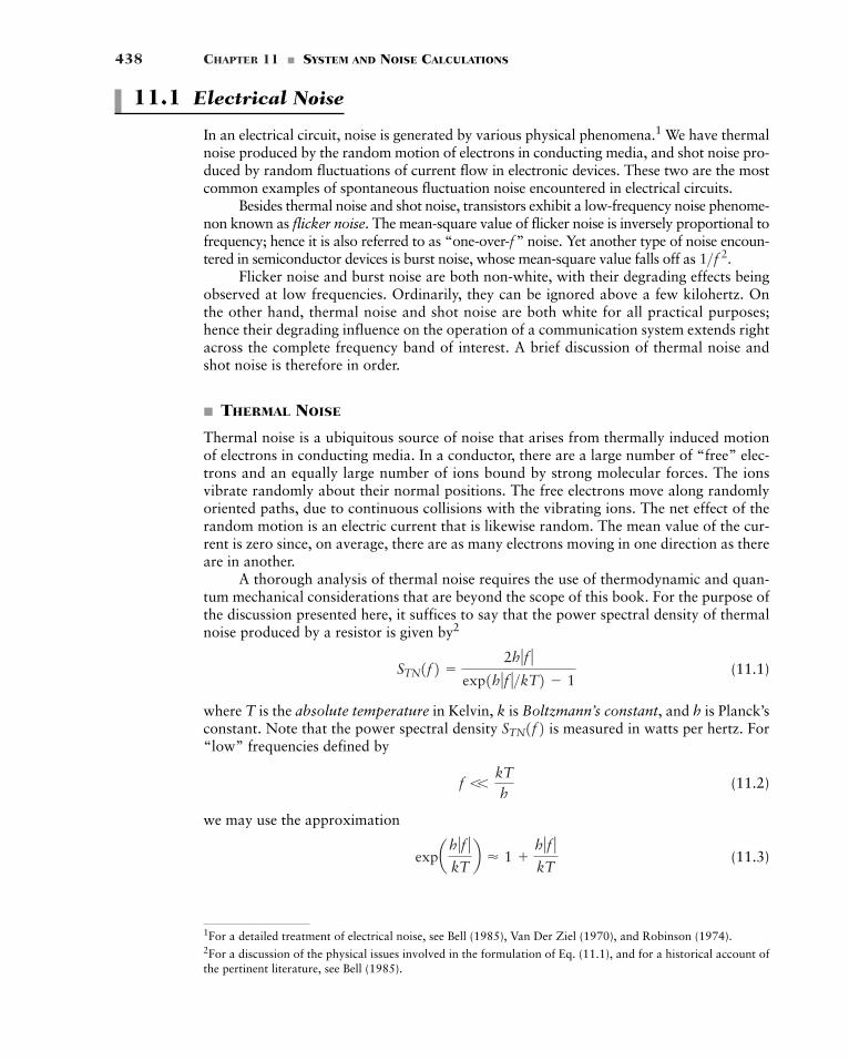
438 CHAPTER 11 � SYSTEM AND NOISE CALCULATIONS
1For a detailed treatment of electrical noise, see Bell (1985), Van Der Ziel (1970), and Robinson (1974).2For a discussion of the physical issues involved in the formulation of Eq. (11.1), and for a historical account ofthe pertinent literature, see Bell (1985).
11.1 Electrical Noise
In an electrical circuit, noise is generated by various physical phenomena.1 We have thermalnoise produced by the random motion of electrons in conducting media, and shot noise pro-duced by random fluctuations of current flow in electronic devices. These two are the mostcommon examples of spontaneous fluctuation noise encountered in electrical circuits.
Besides thermal noise and shot noise, transistors exhibit a low-frequency noise phenome-non known as flicker noise. The mean-square value of flicker noise is inversely proportional tofrequency; hence it is also referred to as “one-over- ” noise. Yet another type of noise encoun-tered in semiconductor devices is burst noise, whose mean-square value falls off as
Flicker noise and burst noise are both non-white, with their degrading effects beingobserved at low frequencies. Ordinarily, they can be ignored above a few kilohertz. Onthe other hand, thermal noise and shot noise are both white for all practical purposes;hence their degrading influence on the operation of a communication system extends rightacross the complete frequency band of interest. A brief discussion of thermal noise andshot noise is therefore in order.
� THERMAL NOISE
Thermal noise is a ubiquitous source of noise that arises from thermally induced motionof electrons in conducting media. In a conductor, there are a large number of “free” elec-trons and an equally large number of ions bound by strong molecular forces. The ionsvibrate randomly about their normal positions. The free electrons move along randomlyoriented paths, due to continuous collisions with the vibrating ions. The net effect of therandom motion is an electric current that is likewise random. The mean value of the cur-rent is zero since, on average, there are as many electrons moving in one direction as thereare in another.
A thorough analysis of thermal noise requires the use of thermodynamic and quan-tum mechanical considerations that are beyond the scope of this book. For the purpose ofthe discussion presented here, it suffices to say that the power spectral density of thermalnoise produced by a resistor is given by2
(11.1)
where T is the absolute temperature in Kelvin, k is Boltzmann’s constant, and h is Planck’sconstant. Note that the power spectral density is measured in watts per hertz. For“low” frequencies defined by
(11.2)
we may use the approximation
(11.3)expah ƒf ƒkTb � 1
h ƒf ƒkT
f VkTh
STN1f2
STN1f2 �2h ƒf ƒ
exp1h ƒf ƒ>kT2 � 1
1>f 2.f
11.1 Electrical Noise 439
(b)
GITN
(a)
R
VTN
FIGURE 11.1 Models of a noisy resistor: (a) Thévenin equivalent circuit and (b) Nortonequivalent circuit.
Substituting this approximate formula into Eq. (11.1) we arrive at the correspondingapproximate formula for the power spectral density of thermal noise:
(11.4)
By substituting the values for Boltzmann’s constant, watts/Hz/ºK,Planck’s constant, watt-(second) , we find that, at a nominal tempera-ture of (17 ºC),
(11.5)
This upper frequency limit lies in the infrared region of the electromagnetic spectrum thatis well above the frequencies encountered in conventional electrical communication systems.Therefore, for all practical purposes the use of the formula of Eq. (11.4) is justified.
Thus given a resistor of R ohms, we find from Eq. (11.4) that the mean-square valueof the thermal noise voltage measured across the terminals of the resistor equals
(11.6)
where is the bandwidth (in hertz) over which the noise voltage is measured. The factor 2in the first line of Eq. (11.6) comes from the fact that the spectral density has both positiveand negative frequencies. We may thus model a noisy resistor by the Thévenin equivalent cir-cuit consisting of a noise voltage generator with a mean square value of in serieswith a noiseless resistor, as in Fig. 11.1(a). Alternatively, we may use the Norton equivalentcircuit consisting of a noise current generator in parallel with a noiseless conductance as in Fig. 11.1(b). The mean-square value of the noise current generator is
(11.7)
Since the number of electrons in a resistor is very large and their random motions insidethe resistor are statistically independent of each other, the central limit theorem indicatesthat thermal noise is Gaussian distributed. Accordingly, for the band of frequencies encoun-tered in electrical communication systems, we may model thermal noise as white Gauss-ian noise of zero mean.
EXAMPLE 11.1 Noise Voltage in AM Radio
The front-end filter of a radio passes the broadcast AM band from 535 kHz to 1605 kHz.The radio input has an effective resistance of 300 ohms. What is the root-mean-square noisevoltage that we would expect to observe due to this resistance?
� 4kTGBN amps2
E3ITN2 4 �
1
R2 E3VTN2 4
G � 1/R,
E3VTN2 4
BN
� 4kTRBN volts2E3VTN
2 4 � 2RBNSTN1f2
kTh
� 6 1012 Hz
T � T0 � 290 K
2h � 6.63 10�34k � 1.38 10�23
STN1f2 � 2kT
440 CHAPTER 11 � SYSTEM AND NOISE CALCULATIONS
From Eq. (11.6), the mean-square thermal noise voltage at room temperature is
Hence, the root-mean-square thermal noise voltage is 2.3 microvolts.
� AVAILABLE NOISE POWER
Noise calculations involve the transfer of power from a source to a load, so we find thatthe use of the maximum-power transfer theorem is applicable. This theorem states thatthe maximum possible power is transferred from a source of internal resistance R to a loadof resistance when Under this matched condition, the power produced by thesource is divided equally between the internal resistance of the source and the load resis-tance. The power delivered to the load is referred to as the available power. Applying themaximum-power transfer theorem to the Thévenin equivalent circuit of Fig. 11.1(a) or theNorton equivalent circuit of Fig. 11.1(b), we readily find that a noisy resistor produces anavailable power equal to watts.
EXAMPLE 11.2 Noise Power
What is the available noise power produced by a 10 kilo-ohm resistor over the bandwidthfrom 0 to 10 MHz?
The available noise power at room temperature is
The root-mean-square (rms) voltage this power produces across a matched load of 10 kilo-ohms is
� Drill Problem 11.1 What is the root-mean-square voltage across a 10 mega-ohm resis-tor at room temperature if it is measured over a 1 GHz bandwidth? What is the available noisepower? �
� SHOT NOISE
Shot noise arises in electronic devices due to the discrete nature of current flow in the device.The process assumes the existence of an average current flow that manifests itself in theform of electrons flowing from the cathode to the plate in vacuum tubes; holes and electronsflowing in semi-conductor devices; and photons emitted in photodiodes. Although the aver-age number of particles moving across the device per unit time is assumed to be constant,the process of current flow through the device exhibits fluctuations about the average value.The manner in which these fluctuations arise varies from one device to another. In a vacuum-tube device, the fluctuations are produced by the random emission of electrons from thecathode. In a semiconductor device, the cause is the random diffusion of electrons or the
� 20.0 microvoltsVrms � 2PNR
� 4.0 10�14 watts
� (1.38 10�23) 290 107
PN � kTBN
kTBN
Rl � R.Rl
� 5.14 10�12 volts2
� 4 (1.38 10�23) 290 300 (1070 103)E3VTN
2 4 � 4kTRBN
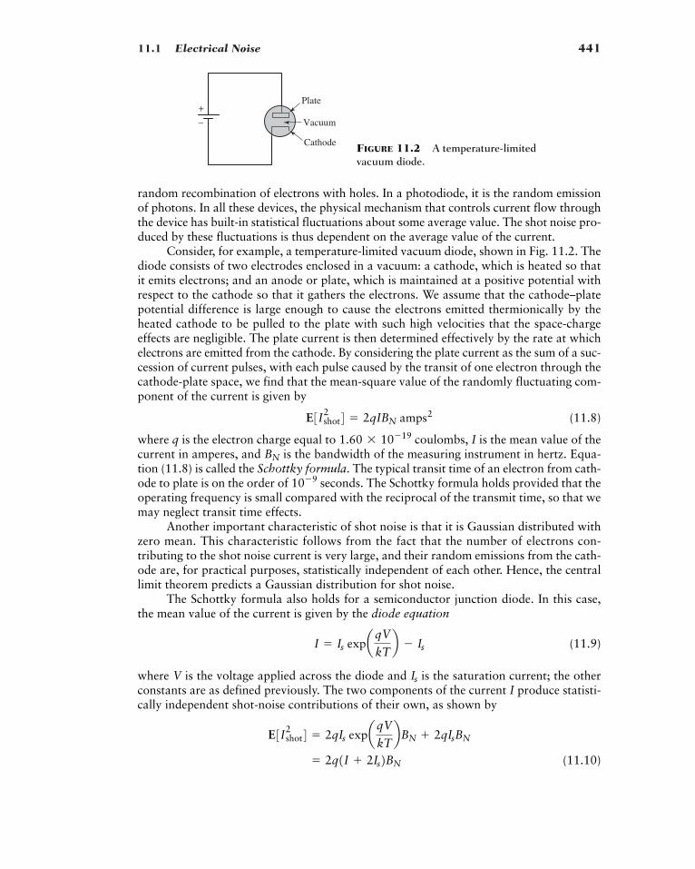
11.1 Electrical Noise 441
Plate
Vacuum
Cathode
+
–
random recombination of electrons with holes. In a photodiode, it is the random emissionof photons. In all these devices, the physical mechanism that controls current flow throughthe device has built-in statistical fluctuations about some average value. The shot noise pro-duced by these fluctuations is thus dependent on the average value of the current.
Consider, for example, a temperature-limited vacuum diode, shown in Fig. 11.2. Thediode consists of two electrodes enclosed in a vacuum: a cathode, which is heated so thatit emits electrons; and an anode or plate, which is maintained at a positive potential withrespect to the cathode so that it gathers the electrons. We assume that the cathode–platepotential difference is large enough to cause the electrons emitted thermionically by theheated cathode to be pulled to the plate with such high velocities that the space-chargeeffects are negligible. The plate current is then determined effectively by the rate at whichelectrons are emitted from the cathode. By considering the plate current as the sum of a suc-cession of current pulses, with each pulse caused by the transit of one electron through thecathode-plate space, we find that the mean-square value of the randomly fluctuating com-ponent of the current is given by
(11.8)
where q is the electron charge equal to coulombs, I is the mean value of thecurrent in amperes, and is the bandwidth of the measuring instrument in hertz. Equa-tion (11.8) is called the Schottky formula. The typical transit time of an electron from cath-ode to plate is on the order of seconds. The Schottky formula holds provided that theoperating frequency is small compared with the reciprocal of the transmit time, so that wemay neglect transit time effects.
Another important characteristic of shot noise is that it is Gaussian distributed withzero mean. This characteristic follows from the fact that the number of electrons con-tributing to the shot noise current is very large, and their random emissions from the cath-ode are, for practical purposes, statistically independent of each other. Hence, the centrallimit theorem predicts a Gaussian distribution for shot noise.
The Schottky formula also holds for a semiconductor junction diode. In this case,the mean value of the current is given by the diode equation
(11.9)
where V is the voltage applied across the diode and is the saturation current; the otherconstants are as defined previously. The two components of the current I produce statisti-cally independent shot-noise contributions of their own, as shown by
(11.10)� 2q1I 2Is2BN
E3Ishot2 4 � 2qIs expaqV
kTbBN 2qIsBN
Is
I � Is expaqV
kTb � Is
10�9
BN
1.60 10�19
E3Ishot2 4 � 2qIBN amps2
FIGURE 11.2 A temperature-limitedvacuum diode.
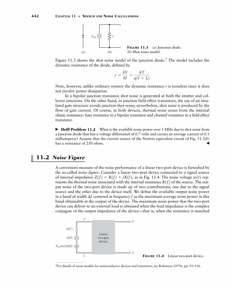
442 CHAPTER 11 � SYSTEM AND NOISE CALCULATIONS
(b)
rISN
(a)FIGURE 11.3 (a) Junction diode.(b) Shot noise model.
Figure 11.3 shows the shot noise model of the junction diode.3 The model includes thedynamic resistance of the diode, defined by
Note, however, unlike ordinary resistor the dynamic resistance r is noiseless since it doesnot involve power dissipation.
In a bipolar junction transistor, shot noise is generated at both the emitter and col-lector junctions. On the other hand, in junction field-effect transistors, the use of an insu-lated gate structure avoids junction shot noise; nevertheless, shot noise is produced by theflow of gate current. Of course, in both devices, thermal noise arises from the internalohmic resistance: base resistance in a bipolar transistor and channel resistance in a field effecttransistor.
� Drill Problem 11.2 What is the available noise power over 1 MHz due to shot noise froma junction diode that has a voltage differential of 0.7 volts and carries an average current of 0.1milliamperes? Assume that the current source of the Norton equivalent circuit of Fig. 11.3(b)has a resistance of 250 ohms. �
11.2 Noise Figure
A convenient measure of the noise performance of a linear two-port device is furnished bythe so-called noise figure. Consider a linear two-port device connected to a signal sourceof internal impedance as in Fig. 11.4. The noise voltage rep-resents the thermal noise associated with the internal resistance R of the source. The out-put noise of the two-port device is made up of two contributions, one due to the signalsource and the other due to the device itself. We define the available output noise powerin a band of width centered at frequency as the maximum average noise power in thisband obtainable at the output of the device. The maximum noise power that the two-portdevice can deliver to an external load is obtained when the load impedance is the complexconjugate of the output impedance of the device—that is, when the resistance is matched
f¢f
1f2 w1t2Z1f2 � R1f2 jX1f2,
r �dVdI
�kT
q1I Is2
1�
1
2�
2
Z(f )
w(t)
~
Lineartwo-portdevice
V0 cos(2�ft)
FIGURE 11.4 Linear two-port device.
3For details of noise models for semiconductor devices and transistors, see Robinson (1974), pp. 93–116.
11.3 Equivalent Noise Temperature 443
and the reactance is tuned out. We define the noise figure of the two-port device as theratio of the total available output noise power (due to the device and the source) per unitbandwidth to the portion thereof due to the source.
Let the spectral density of the total available noise power of the device output beand the spectral density of the available noise power due to the source at the device
input be Also let denote the available power gain of the two-port device,defined as the ratio of the available signal power at the output of the device to the avail-able signal power of the source when the signal is a sinusoidal wave of frequency Thenwe may express the noise figure F of the device as
(11.11)
If the device were noise-free, and the noise figure would thenbe unity. In a physical device, however, is larger than so that the noisefigure is always larger than unity. The noise figure is commonly expressed in decibels—thatis, as
The noise figure F of Eq. (11.11) is a function of the operating frequency it is there-fore referred to as the spot noise figure. In contrast, we may define the average noise fig-ure of a two-port device as the ratio of the total noise power at the device output to theoutput noise power due solely to the source. That is,
(11.12)
It is apparent that, in the case where thermal noise in the input circuit corresponds to a con-stant resistance and the device has a constant gain throughout a fixed band with zerogain at other frequencies, the spot noise figure F and the average noise figure are identical.
EXAMPLE 11.3 Noise Figure Calculation
The input of a two-port network with a gain of 10 dB and a constant noise figure of 8 dB is con-nected to a resistor that generates a power spectral density where is the nom-inal temperature. What is the noise spectral density at the output of the two-port network?
From Eq. (11.11) applied at arbitrary frequency we find that the output noise spec-tral density is
Expressed in decibels, we have
where we have used the fact that
11.3 Equivalent Noise Temperature
A disadvantage of the noise figure F is that, when it is used to compare low-noise devices, thevalues are all close to unity, which makes the comparison difficult. In such cases, it is prefer-able to use the equivalent noise temperature. Consider a linear two-port device whose input
kT0 � 1.38 10�23 290 watts>Hz � �174 dBm>Hz.
� �156 dBm>Hz� 10 8 (�174)
SNO � FdB GdB 1kT02dBm>Hz
SNO1f2 � F1f2G1f2SNS1f2f,
T0SNS1f2 � kT0
F0
R1f2,
F0 �L
q
�qSNO1f2 df
Lq
�qG1f2SNS1f2 df
F0
f;10 log101F2.
G1f2SNS1f2,SNO1f2SNO1f2 � G1f2SNS1f2F1f2 �
SNO1f2G1f2SNS1f2
f.
G1f2SNS1f2.SNO1f2
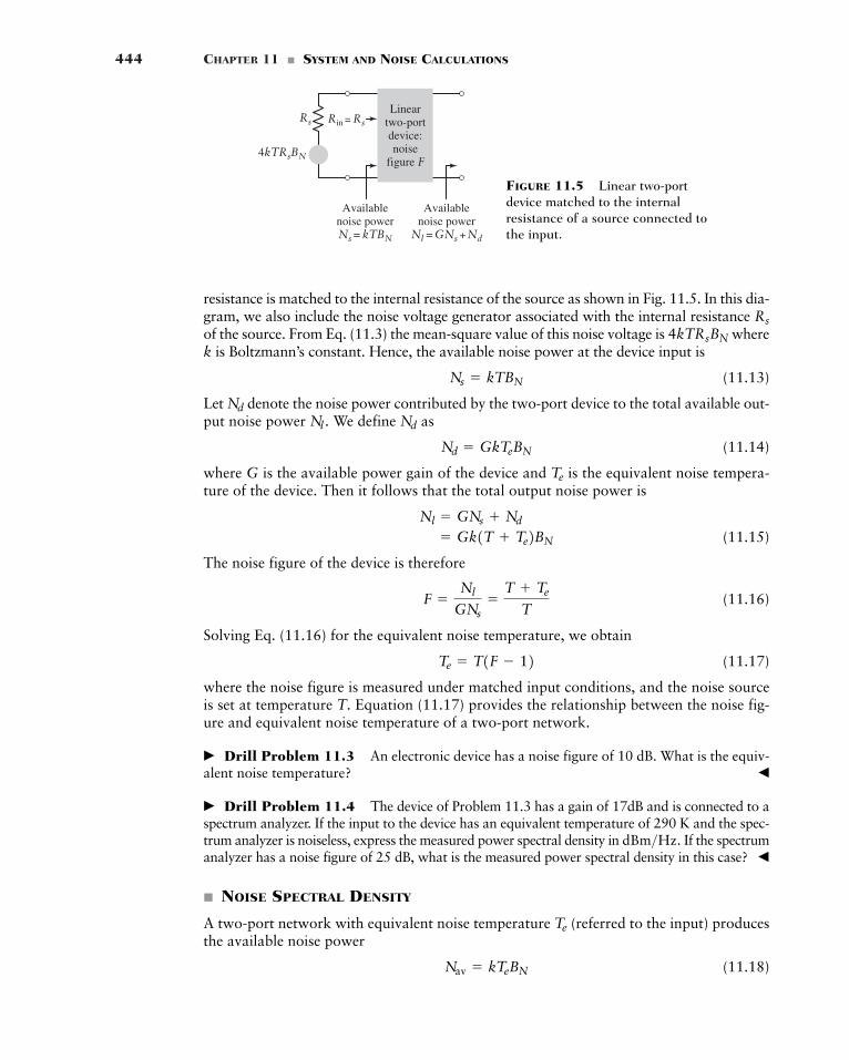
444 CHAPTER 11 � SYSTEM AND NOISE CALCULATIONS
Rs Rin= Rs
Lineartwo-portdevice:noise
figure F
Availablenoise powerNs = kTBN
Availablenoise power
Nl = GNs + Nd
4kTRsBN
FIGURE 11.5 Linear two-portdevice matched to the internalresistance of a source connected tothe input.
resistance is matched to the internal resistance of the source as shown in Fig. 11.5. In this dia-gram, we also include the noise voltage generator associated with the internal resistance of the source. From Eq. (11.3) the mean-square value of this noise voltage is wherek is Boltzmann’s constant. Hence, the available noise power at the device input is
(11.13)
Let denote the noise power contributed by the two-port device to the total available out-put noise power We define as
(11.14)
where G is the available power gain of the device and is the equivalent noise tempera-ture of the device. Then it follows that the total output noise power is
(11.15)
The noise figure of the device is therefore
(11.16)
Solving Eq. (11.16) for the equivalent noise temperature, we obtain
(11.17)
where the noise figure is measured under matched input conditions, and the noise sourceis set at temperature T. Equation (11.17) provides the relationship between the noise fig-ure and equivalent noise temperature of a two-port network.
� Drill Problem 11.3 An electronic device has a noise figure of 10 dB. What is the equiv-alent noise temperature? �
� Drill Problem 11.4 The device of Problem 11.3 has a gain of 17dB and is connected to aspectrum analyzer. If the input to the device has an equivalent temperature of 290 K and the spec-trum analyzer is noiseless, express the measured power spectral density in If the spectrumanalyzer has a noise figure of 25 dB, what is the measured power spectral density in this case? �
� NOISE SPECTRAL DENSITY
A two-port network with equivalent noise temperature (referred to the input) producesthe available noise power
(11.18)Nav � kTeBN
Te
dBm>Hz.
Te � T1F � 12
F �Nl
GNs�
T Te
T
� Gk1T Te2BN
Nl � GNs Nd
Te
Nd � GkTeBN
NdNl .Nd
Ns � kTBN
4kTRsBN
Rs
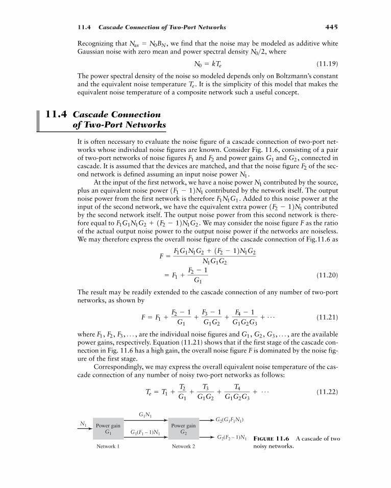
11.4 Cascade Connection of Two-Port Networks 445
Power gainG1
N1
G1N1
G1(F1 – 1)N1G2(F2 – 1)N1
G2(G1F1N1)Power gain
G2
Network 1 Network 2FIGURE 11.6 A cascade of twonoisy networks.
Recognizing that we find that the noise may be modeled as additive whiteGaussian noise with zero mean and power spectral density where
(11.19)
The power spectral density of the noise so modeled depends only on Boltzmann’s constantand the equivalent noise temperature It is the simplicity of this model that makes theequivalent noise temperature of a composite network such a useful concept.
11.4 Cascade Connection of Two-Port Networks
It is often necessary to evaluate the noise figure of a cascade connection of two-port net-works whose individual noise figures are known. Consider Fig. 11.6, consisting of a pairof two-port networks of noise figures and and power gains and connected incascade. It is assumed that the devices are matched, and that the noise figure of the sec-ond network is defined assuming an input noise power
At the input of the first network, we have a noise power contributed by the source,plus an equivalent noise power contributed by the network itself. The outputnoise power from the first network is therefore Added to this noise power at theinput of the second network, we have the equivalent extra power contributedby the second network itself. The output noise power from this second network is there-fore equal to We may consider the noise figure F as the ratioof the actual output noise power to the output noise power if the networks are noiseless.We may therefore express the overall noise figure of the cascade connection of Fig.11.6 as
(11.20)
The result may be readily extended to the cascade connection of any number of two-portnetworks, as shown by
(11.21)
where are the individual noise figures and are the availablepower gains, respectively. Equation (11.21) shows that if the first stage of the cascade con-nection in Fig. 11.6 has a high gain, the overall noise figure F is dominated by the noise fig-ure of the first stage.
Correspondingly, we may express the overall equivalent noise temperature of the cas-cade connection of any number of noisy two-port networks as follows:
(11.22)Te � T1 T2
G1
T3
G1G2
T4
G1G2G3 Á
G1, G2, G3, Á ,F1, F2, F3, Á ,
F � F1 F2 � 1
G1
F3 � 1G1G2
F4 � 1
G1G2G3 Á
� F1 F2 � 1
G1
F �F1G1N1G2 1F2 � 12N1G2
N1G1G2
F1G1N1G2 1F2 � 12N1G2.
1F2 � 12N1
F1N1G1.1F1 � 12N1
N1
N1.F2
G2,G1F2F1
Te .
N0 � kTe
N0>2,Nav � N0BN ,
446 CHAPTER 11 � SYSTEM AND NOISE CALCULATIONS
4For a detailed treatment of link calculations for satellite communications, see Chapter 4 of Pratt and Bostian(1986).5For a detailed treatment of link calculations for deep-space communications, see Chapter 3 of Yuen (1983).
where are the equivalent noise temperatures of the individual networks.From Eq. (11.22) we also see that if the first stage of a cascade connection of noisytwo-port networks has a large power gain, then the overall value of the equivalent noisetemperature is practically the same as that of the first stage. For this reason, in alow-noise receiver, extra care is taken in the design of the pre-amplifier or low-noiseamplifier at the very front end of the receiver.
EXAMPLE 11.4 System Noise Temperature of a Satellite Receiver
A satellite receiver consists of an antenna that has a noise temperature of 50 K. This is followedby a low-noise amplifier with 30 dB of gain and noise temperature of 70 K. The low-noiseamplifier, in turn, is followed by a second stage amplifier with a gain of 40 dB and noise tem-perature of 1500 K. What is the system noise temperature?
For this three-stage system, Eq. (11.22) shows that the system noise temperature is given by
where and are the noise temperatures of the antenna, low-noise amplifier, and sec-ond stage amplifier, respectively. Since the antenna does not provide any electrical gain to thereceived signal, Consequently, the effective noise temperature is
� Drill Problem 11.5 A broadcast television receiver consists of an antenna with a noisetemperature of 290 K and a pre-amplifier with an available power gain of 20 dB and a noisefigure of 9 dB. A second-stage amplifier in the receiver provides another 20 dB of gain and hasa noise figure of 20 dB. What is the noise figure of the overall system? �
11.5 Free-Space Link Calculations
In this section, we move on to the issue of signal and noise power calculations for radio linksthat rely on line-of-sight propagation through space. Such calculations are encountered insatellite communications,4 for example. In a satellite system, the message signal is trans-mitted from a ground station via the uplink to a geosynchronous satellite, amplified in atransponder therein, and then retransmitted from the satellite via the downlink to anotherground Earth station. The satellite is positioned in a geostationary orbit (around the Earth)so that it is always visible to different ground stations located inside the satellite antenna’scoverage zone on the Earth’s surface. The satellite, in effect, acts as a repeater in the sky.Another application with line-of-sight propagation characteristics is deep-space commu-nication5 of information between a spacecraft and a ground station. In this second appli-cation, the system includes a tracking capability such that the spacecraft is always visibleto one of multiple ground stations. For the analysis presented here, we will consider the satel-lite link as illustrative of space applications.
� 121.5 K
Te � 50 701
1500
1 1000
G1 � 1.
T3T1, T2,
Te � T1 T2
G1
T3
G1G2
Te
T1, T2, T3, Á ,

11.5 Free-Space Link Calculations 447
Low-noisereceiver Output
Earth-stationantenna
Antenna
Spacecraft
� CALCULATION OF RECEIVED SIGNAL POWER
Figure 11.7 illustrates a down-link between a spacecraft and a ground Earth station. Thelink includes a transmitting source (on the spacecraft) with its output radiated through thespacecraft’s antenna. At the ground station, a receiving antenna is used to collect signalpower from the incoming electromagnetic wave and feed it to the low-noise receiver througha waveguide.
Let the transmitting source radiate a total power If this power is radiated isotropi-cally (i.e., uniformly in all directions), the power flux density at a distance r from the sourceis where is the surface area of a sphere of radius r. In practice, we use a highlydirectional antenna so that the transmitted power is radiated primarily along a particular direc-tion of interest. The antenna has a gain that is defined as the ratio of power radiated per unitsolid angle in a given direction to the average power radiated per solid angle. Let denotethe gain of the transmitting antenna in the direction in which the maximum power is radiated;this direction is called the boresight of the antenna. The gain is a measure of the increasein power radiated by the antenna over that radiated by an isotropic source. Thus for a trans-mitter of total power driving a lossless antenna with gain the power flux density at dis-tance r in the direction of the antenna boresight is given by
(11.23)
Let denote the effective aperture area of the receiving antenna. This area is relatedto the physical aperture area A of the antenna by the formula
(11.24)
where is the aperture efficiency. Typically is in the range of 40 to 90 percent, depend-ing on the type of antenna employed. The gain of the receiving antenna is defined interms of the effective aperture by
(11.25)
where is the wavelength of the transmitted electromagnetic wave; is equal to wherec is the speed of propagation (which is the same as the speed of light), and is thetransmission frequency. Equivalently, we have
(11.26)Aeff �GRl
2
4p
fc>fll
GR �4pAeff
l2
Aeff
GR
hh
Aeff � hA
Aeff
£ �PTGT
4pr2
GT ,PT
GT
GT
4pr2PT>14pr22,PT .
FIGURE 11.7 Space communication down-link.
448 CHAPTER 11 � SYSTEM AND NOISE CALCULATIONS
6There are exceptions to this rule, most notably satellite-to-mobile terminal communications and direct-to-home satellite television broadcasts.
Hence, given the power flux density at the receiving antenna with an effective aperturearea the received power is
(11.27)
Thus, substituting Eqs. (11.23) and (11.26) into (11.27), we obtain the result
(11.28)
Equation (11.28) is known as the Friis transmission formula, which relates the receivedpower to the transmitted power. The product in this equation is called the effectiveisotropic radiated power (EIRP). It describes the combination of the transmitting source andantenna in terms of an effective isotropic source with power radiated uniformly inall directions. The term is called the path loss or free-space loss; it may be viewedas the ratio of transmitted power to received power between two antennas that are sepa-rated by a distance r.
From Eq. (11.28) we see that for given values of wavelength and distance r, thereceived power may be increased by three methods:
1. The spacecraft-transmitted power is increased. The transmitted power may be20 watts or less. Even though this transmitted power may appear low, the input powerrequired for its generation represents a substantial fraction of the total power avail-able on the spacecraft. Hence, there is a physical limit on how large a value we canassign to the transmitted power
2. The gain of the transmitting antenna is increased. This will help concentrate thetransmitted power rather intensely in the direction of the receiving antenna. However,a large value of requires the use of a large antenna. The choice of is thereforelimited by size and weight constraints of the spacecraft.
3. The gain of the receiving antenna is increased. This will enable the receiver tocollect as much of the radiated signal power as possible. Here again, size and weightconstraints place a physical limit on the size of the ground-station antenna, althoughthese constraints are far less demanding than those on the spacecraft antenna; wetypically6 have
Let the receiving antenna gain and space loss be expressed in decibels (dB). Likewise,let the effective radiated power and the received power be expressed in decibels relative toone watt (dBW). Then we may restate the Friis transmission formula in the form
(11.29)
where
(11.30)
(11.31)
(11.32)
In Eq. (11.25), is represented as a power ratio, whereas in Eq. (11.31) it isexpressed in decibels. Equation (11.29) is idealized in that it does not account for all losses
GR
Lp � 20 log10a4prlb
GR � 10 log10¢4pAeff
l2 ≤EIRP � 10 log101PTGT2PR � EIRP GR � Lp
GR W GT .
GR
GTGT
GT
PT .
PTPT
l
14pr>l22 PTGT
PTGT
PR � PTGTGRa l4prb2
PR � Aeff£
Aeff ,£
11.5 Free-Space Link Calculations 449
in the link. To correct for this, it is customary to include a term that represents the com-bined effect of losses in the atmosphere due to rain attenuation, losses in the transmittingand receiving antennas, and possible loss of gain due to mispointing of the antennas. Let
denote the overall value of this loss expressed in decibels; this term is sometimes calledthe system margin. Then we may modify the expression for the received signal power as
(11.33)
Equation (11.33) represents the link (power) budget in that it allows the system designerof a telecommunication link to adjust controllable parameters such as EIRP or the receiv-ing antenna gain and make quick calculations of the received power.
The received power is commonly called the carrier power. This nomenclature isderived from early satellite systems where phase or frequency modulation was commonlyemployed. Since these modulation strategies maintain the envelope of the sinusoidal car-rier constant, the carrier power is typically equal to the received power.
EXAMPLE 11.5 Satellite Link Budget
A geostationary satellite is located at a distance of 40,000 km from an Earth station. At thesatellite a source at a frequency of 4 GHz radiates a power of 10 watts through an antenna witha gain of 20 dB. Assume that the effective aperture area of the receiving antenna is Cal-culate the received signal power, ignoring nonideal losses in the links.
The effective radiated power with and is
The speed of propagation equals the speed of light: The wavelength of thetransmitted 4 GHz electromagnetic wave is therefore
Hence, the path loss equals
The gain of the receiving antenna with is
� 43.5 dB
� 10 log10¢4p 10
0.0752 ≤GR � 10 log10¢4pAeff
l2 ≤Aeff � 10 m2
� 196.5 dB
� 20 log10a4p 4 107
0.075b
Lp � 20 log10a4prlb
� 0.075 m
�3 108
4 109
l �cf
c � 3 108 m>s.� 30 dBW� 10 log1010 20� 10 log10 PT 10 log10 GT
EIRP � 10 log101PTGT2GT � 20 dBPT � 10 W
10 m2.
PR
GR
PR � EIRP GR � Lp � L0
L0
450 CHAPTER 11 � SYSTEM AND NOISE CALCULATIONS
Thus, using Eq. (11.29) and ignoring the system margin we find that the received signalpower equals
Equivalently, the received power may be written as watts. The low value of indicates that the received signal at the Earth station is extremely weak. Other losses on the link(accounted for in the system margin) at the Earth station will make the received signal even weaker.
� Drill Problem 11.6 A satellite antenna has a diameter of 4.6 meters and operates at 12GHz. What is the antenna gain if the aperture efficiency is 60 percent? If the same antenna wasused at 4 GHz, what would be the corresponding gain? �
� Drill Problem 11.7 A satellite at a distance of 40,000 kilometers transmits a signal at12 GHz with an EIRP of 10 watts toward a 4.6 meter antenna that has an aperture efficiencyof 60 percent. What is the received signal level at the antenna output? �
� CARRIER-TO-NOISE RATIO
The carrier-to-noise ratio (CNR) is defined as the ratio of carrier power to the available noisepower, with both measured at the receiver input. As mentioned previously, the carrierpower is the same as the received signal power The formula for is described by theFriis transmission equation (11.28). To calculate the available noise power at the receiverinput, we use the expression where k is Boltzmann’s constant, is the system noisetemperature, and is the noise bandwidth. We therefore have
(11.34)
Here again, the simplicity of this formula stems from the use of noise temperature as themeasure of how noisy the system is. The carrier-to-noise ratio is often the same as the pre-detection SNR discussed in Chapter 9.
EXAMPLE 11.6 Calculation of CNR
Consider an Earth station receiver with a cryogenically cooled amplifier. The equivalent noisetemperature of the receiver is 20K. The Earth station uses a large antenna operating at a fre-quency of 4 GHz and an elevation of 15 degrees; the antenna noise temperature is estimatedto be 50K. Calculate the system noise temperature, assuming no loss in the antenna feed andwaveguide. Then calculate the carrier-to-noise ratio, assuming a carrier power of (as in Example 11.5) and a noise bandwidth of 36 MHz.
From Eq. (11.22), we see that with the system noise temperature equals
The available noise power in the 36 MHz bandwidth is therefore
� �134.6 dBW
� 3.48 10�14 W
kTsBN � 1.38 10�23 70 (36 106)
� 70 K� 50 20
Ts � Ta Te
G1 � 1
�123 dBW
CNR �PR
kTsBN
BN
TskTsBN ,
PRPR .
PRPR � 5 10�13
� �123 dBW
PR � 30 43.5 � 196.5
L0,
11.6 Terrestrial Mobile Radio 451
7See Chapter 2 of Haykin and Moher (2004) for further details.
Thus the use of Eq. (11.34) yields the following value for the carrier-to-noise ratio expressedin decibels:
Recall from our discussion of analog receivers in Chapter 9 that this CNR would just be suf-ficient to operate an FM system at threshold. In contrast, this CNR would provide a satisfac-tory bit error rate for many digital systems.
� Drill Problem 11.8 The antenna of Problem 11.7 has a noise temperature of 70 K and isdirectly connected to a receiver with an equivalent noise temperature of 50 K and a gain of 60 dB.What is the system noise temperature? If the transmitted signal has a bandwidth of 100 kHz, whatis the carrier-to-noise ratio? If the digital signal has a bit rate of 150 kbps, what is �
11.6 Terrestrial Mobile Radio
Free-space propagation is often a good model for satellite communications where there isa clear line-of-sight between the transmitter and the receiver. It also provides insight becausethere is a simple theoretical explanation for propagation losses.
With terrestrial communications, on the other hand, both antennas are usually rela-tively close to the ground. Consequently, buildings, terrain, and vegetation may obstructthe line-of-sight path. Terrestrial radio communication often relies on the reflection of elec-tromagnetic waves from various surfaces or diffraction of these waves around variousobjects. With these additional modes of propagation, there are a multitude of possiblepropagation paths between the transmitter and receiver, and the receiver often receives asignificant signal from more than one path. This phenomenon is referred to as multipathpropagation. With multiple waves arriving at the same location, propagation properties maydiffer significantly from free-space propagation.
There are three basic propagation modes that apply to terrestrial propagation: free-space, reflection, and diffraction.7
1. Free-space propagation depends upon a line-of-sight path between the transmitterand the receiver and a certain clearance around that path. The required clearance, illus-trated in Fig. 11.8, is related to the separation of the two, and the wavelength oftransmission. A rule of thumb is that a volume known as the first Fresnel zone mustbe kept clear of objects for approximate free-space propagation. The Fresnel zonedefines an ellipsoid of revolution. Objects within the first Fresnel zone will affecttransmission and cause deviation from the free-space propagation model. The radiusof the first Fresnel zone varies with the position between the transmitting and receiv-ing antenna; it is given by
(11.35)
where is the wavelength of transmission, is the distance to the transmitter, andis the distance to the receiver, for the particular point along the path.d2
d1l
h � B ld1d2
d1 d2
Eb>N0?
� 11.6 dB10 log101CNR2 � �123 134.6
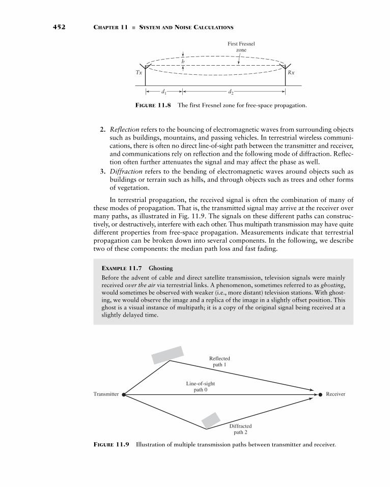
452 CHAPTER 11 � SYSTEM AND NOISE CALCULATIONS
Transmitter Receiver
Reflectedpath 1
Line-of-sightpath 0
Diffractedpath 2
FIGURE 11.9 Illustration of multiple transmission paths between transmitter and receiver.
First Fresnelzone
h
d1
Tx Rx
d2
FIGURE 11.8 The first Fresnel zone for free-space propagation.
2. Reflection refers to the bouncing of electromagnetic waves from surrounding objectssuch as buildings, mountains, and passing vehicles. In terrestrial wireless communi-cations, there is often no direct line-of-sight path between the transmitter and receiver,and communications rely on reflection and the following mode of diffraction. Reflec-tion often further attenuates the signal and may affect the phase as well.
3. Diffraction refers to the bending of electromagnetic waves around objects such asbuildings or terrain such as hills, and through objects such as trees and other formsof vegetation.
In terrestrial propagation, the received signal is often the combination of many ofthese modes of propagation. That is, the transmitted signal may arrive at the receiver overmany paths, as illustrated in Fig. 11.9. The signals on these different paths can construc-tively, or destructively, interfere with each other. Thus multipath transmission may have quitedifferent properties from free-space propagation. Measurements indicate that terrestrialpropagation can be broken down into several components. In the following, we describetwo of these components: the median path loss and fast fading.
EXAMPLE 11.7 Ghosting
Before the advent of cable and direct satellite transmission, television signals were mainlyreceived over the air via terrestrial links. A phenomenon, sometimes referred to as ghosting,would sometimes be observed with weaker (i.e., more distant) television stations. With ghost-ing, we would observe the image and a replica of the image in a slightly offset position. Thisghost is a visual instance of multipath; it is a copy of the original signal being received at aslightly delayed time.
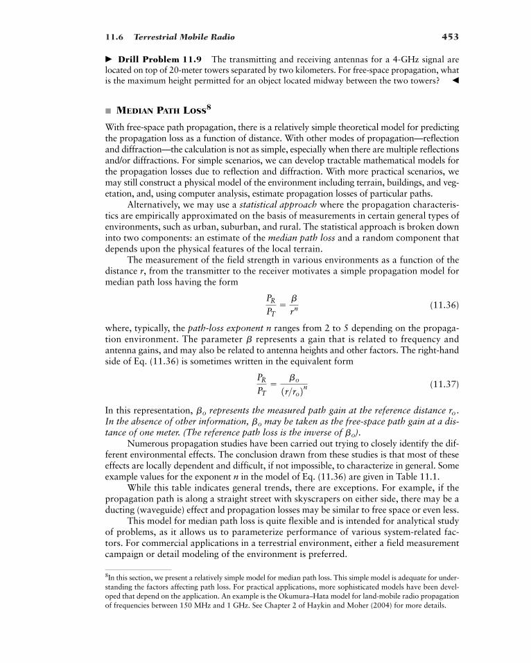
11.6 Terrestrial Mobile Radio 453
8In this section, we present a relatively simple model for median path loss. This simple model is adequate for under-standing the factors affecting path loss. For practical applications, more sophisticated models have been devel-oped that depend on the application. An example is the Okumura–Hata model for land-mobile radio propagationof frequencies between 150 MHz and 1 GHz. See Chapter 2 of Haykin and Moher (2004) for more details.
� Drill Problem 11.9 The transmitting and receiving antennas for a 4-GHz signal arelocated on top of 20-meter towers separated by two kilometers. For free-space propagation, whatis the maximum height permitted for an object located midway between the two towers? �
� MEDIAN PATH LOSS8
With free-space path propagation, there is a relatively simple theoretical model for predictingthe propagation loss as a function of distance. With other modes of propagation—reflectionand diffraction—the calculation is not as simple, especially when there are multiple reflectionsand/or diffractions. For simple scenarios, we can develop tractable mathematical models forthe propagation losses due to reflection and diffraction. With more practical scenarios, wemay still construct a physical model of the environment including terrain, buildings, and veg-etation, and, using computer analysis, estimate propagation losses of particular paths.
Alternatively, we may use a statistical approach where the propagation characteris-tics are empirically approximated on the basis of measurements in certain general types ofenvironments, such as urban, suburban, and rural. The statistical approach is broken downinto two components: an estimate of the median path loss and a random component thatdepends upon the physical features of the local terrain.
The measurement of the field strength in various environments as a function of thedistance r, from the transmitter to the receiver motivates a simple propagation model formedian path loss having the form
(11.36)
where, typically, the path-loss exponent n ranges from 2 to 5 depending on the propaga-tion environment. The parameter represents a gain that is related to frequency andantenna gains, and may also be related to antenna heights and other factors. The right-handside of Eq. (11.36) is sometimes written in the equivalent form
(11.37)
In this representation, represents the measured path gain at the reference distanceIn the absence of other information, may be taken as the free-space path gain at a dis-tance of one meter. (The reference path loss is the inverse of ).
Numerous propagation studies have been carried out trying to closely identify the dif-ferent environmental effects. The conclusion drawn from these studies is that most of theseeffects are locally dependent and difficult, if not impossible, to characterize in general. Someexample values for the exponent n in the model of Eq. (11.36) are given in Table 11.1.
While this table indicates general trends, there are exceptions. For example, if thepropagation path is along a straight street with skyscrapers on either side, there may be aducting (waveguide) effect and propagation losses may be similar to free space or even less.
This model for median path loss is quite flexible and is intended for analytical studyof problems, as it allows us to parameterize performance of various system-related fac-tors. For commercial applications in a terrestrial environment, either a field measurementcampaign or detail modeling of the environment is preferred.
bo
bo
ro .bo
PR
PT�
bo1r>ro2n
b
PR
PT�b
rn
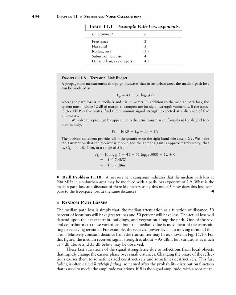
454 CHAPTER 11 � SYSTEM AND NOISE CALCULATIONS
TABLE 11.1 Example Path-Loss exponents.
Environment n
Free space 2Flat rural 3Rolling rural 3.5Suburban, low rise 4Dense urban, skyscrapers 4.5
EXAMPLE 11.8 Terrestrial Link Budget
A propagation measurement campaign indicates that in an urban area, the median path losscan be modeled as
where the path loss is in decibels and r is in meters. In addition to the median path loss, thesystem must include 12 dB of margin to compensate for signal strength variations. If the trans-mitter EIRP is five watts, find the minimum signal strength expected at a distance of fivekilometers.
We solve this problem by appealing to the Friis transmission formula in the decibel for-mat; namely,
The problem statement provides all of the quantities on the right-hand side except We makethe assumption that the receiver is mobile and the antenna gain is approximately unity; thatis, Then, at a range of 5 km,
� Drill Problem 11.10 A measurement campaign indicates that the median path loss at900 MHz in a suburban area may be modeled with a path-loss exponent of 2.9. What is themedian path loss at a distance of three kilometers using this model? How does this loss com-pare to the free-space loss at the same distance? �
� RANDOM PATH LOSSES
The median path loss is simply that: the median attenuation as a function of distance; 50percent of locations will have greater loss and 50 percent will have less. The actual loss willdepend upon the exact terrain, buildings, and vegetation along the path. One of the sev-eral contributors to these variations about the median value is movement of the transmit-ting or receiving terminal. For example, the received power level at a moving terminal thatis at a relatively constant distance from the transmitter may be as shown in Fig. 11.10. Forthis figure, the median received signal strength is about but variations as muchas 7 dB above and 35 dB below may be observed.
These fast variations of the signal strength are due to reflections from local objectsthat rapidly change the carrier phase over small distances. Changing the phase of the reflec-tions causes them to sometimes add constructively and sometimes destructively. This fastfading is often called Rayleigh fading, so named after the probability distribution functionthat is used to model the amplitude variations. If R is the signal amplitude, with a root-mean-
�95 dBm,
� �130.7 dBm� �160.7 dBW
PR � 10 log10 5 � 41 � 31 log10 5000 � 12 0
GR � 0 dB.
GR .
PR � EIRP � Lp � L0 GR
Lp � 41 31 log101r2
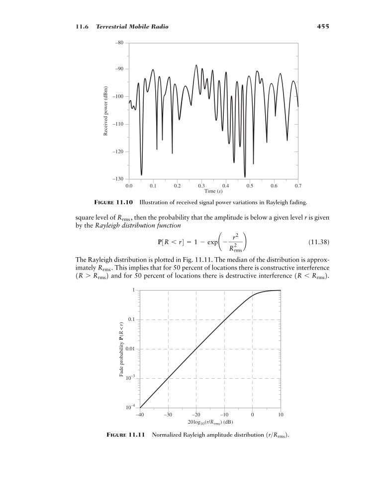
11.6 Terrestrial Mobile Radio 455
Rec
eive
d po
wer
(dB
m)
Time (s)0.0 0.1 0.2 0.3 0.4 0.5 0.6 0.7
–130
–120
–110
–100
–90
–80
FIGURE 11.10 Illustration of received signal power variations in Rayleigh fading.
Fade
pro
babi
lity
P(R
<r)
20 log10(r/Rrms) (dB)–40 –30 –20 –10 0 10
10–4
10–3
0.01
0.1
1
FIGURE 11.11 Normalized Rayleigh amplitude distribution 1r>Rrms2.
square level of then the probability that the amplitude is below a given level r is givenby the Rayleigh distribution function
(11.38)
The Rayleigh distribution is plotted in Fig. 11.11. The median of the distribution is approx-imately This implies that for 50 percent of locations there is constructive interference
and for 50 percent of locations there is destructive interference 1R � Rrms2.1R � Rrms2Rrms .
P3R � r4 � 1 � exp¢�r2
Rrms2 ≤
Rrms ,
456 CHAPTER 11 � SYSTEM AND NOISE CALCULATIONS
Deep fades of 20 dB or more occur only rarely (with a probability of 1 per-cent). However, Fig. 11.11 indicates that there can be a wide variation in received signalstrength due to local reflections.
EXAMPLE 11.9 Margin for Rayleigh Fading
Suppose a mobile radio has a receiver sensitivity of That is, is the mini-mum signal level that the receiver can reliably the demodulate. The system operates at 900MHz and the intended range is 2 kilometers. Find the transmitter power required to serve thisreceiver if the propagation environment has a path-loss exponent n 2.9 and the receivermust tolerate 90 percent of the fades.
If the receiver must tolerate 90 percent of the fades, then the Rayleigh distribution func-tion of Fig. 11.11 indicates that the system should include 10 dB of margin. Consequently, themedian signal level should be 10 dB above the receiver sensitivity at the edge of coverage—thatis, Then using Eq. (11.37), we have
We assume is the free-space path gain at one meter, so
at 900 MHz. Expressing the above equation for in decibel format, we obtain
This corresponds to approximately a 50-watt transmitter.
� Drill Problem 11.11 Express the true median of the Rayleigh distribution as a fractionof the value? What is the decibel error in the approximation �
11.7 Summary and Discussion
In this chapter, we have characterized specific sources of noise and signal attenuation in prac-tical communication systems. These are the inputs required to calculate the signal-to-noiseratios used to characterize receiver performance in previous chapters. In particular:
(i) Several sources of thermal noise were identified, and we characterized their powerspectral densities through the simple relation where k is Boltzmann’s con-stant and T is the absolute temperature in Kelvin.
(ii) The related concepts of noise figure and equivalent noise temperature were definedand used to characterize the contributions that various electronic devices or noisesources make to the overall noise. We then showed how the overall noise is calculatedin a cascaded two-port system.
N0 � kT,
Rmedian � Rrms?Rrms
� 47 dBm
� �80 31.5 95.7
PT � PR � b0 29 log10a20001b
PT
� �31.5 dB
bo (dB) � �Lp (1m) � �20 log10a4plb
bo
PT �PR
b0
1r>ro22.9
�80 dBm.
�
�90 dBm�90 dBm.
1R � 0.1Rrms2
Additional Problems 457
(iii) The Friis equation was developed to mathematically model the relationship betweentransmitted and received signal strengths as a function of transmitting and receivingantenna gains and path loss.
(iv) Propagation losses ranging from free-space conditions, typical of satellite channels,to those typical of terrestrial mobile applications were described. Variations aboutmedian path loss were identified as an important consideration in terrestrialpropagation.
This chapter has provided a brief introduction to two communication channels—satellite and terrestrial—and the effects that propagation and noise have on communica-tion performance. The propagation loss of the channel is a key component in determiningthe signal power at the receiver. The physical noise sources are the contributors to the noisepower at the receiver. The combination of these two quantities—that is, the ratio of the sig-nal power to the noise power—forms the primary method of assessing the quality of acommunication link.
ADDITIONAL PROBLEMS
11.12 Compute the noise spectral density in watts per hertz of:
(a) An ideal resistor at nominal temperature of 290 K.
(b) An amplifier with an equivalent noise temperature of 22,000 K.
11.13 For the two cases of Problem 11.12, compute the pre-detection SNR when the received signalpower is:
(a) and the receive bandwidth is 1 MHz.
(b) and the receive bandwidth is 30 kHz.
Express the answers in both absolute terms and decibels.
11.14 A wireless local area network transmits a signal that has a noise bandwidth of approximately6 MHz. If the signal strength at the receiver input terminals is and the receiver noisefigure is 8 dB, what is the pre-detection signal-to-noise ratio?
11.15 A communications receiver includes a whip antenna whose noise temperature is approximatelythat of the Earth—that is, 290 K. The receiver pre-amplifier has a noise figure of 4 dB and a gainof 25 dB. Calculate (a) the equivalent noise temperature of the antenna and the pre-amplifier,and (b) the combined noise figure.
11.16 A parabolic antenna with a diameter of 0.75 meters is used to receive a 12 GHz satellite signal.Calculate the gain in decibels of this antenna. Assume that the antenna efficiency is 60 percent.
11.17 If the system noise temperature of a satellite receiver is 300 K, what is the required received sig-nal strength to produce a of 80 dB?
11.18 If a satellite is 40,000 km from the antenna of Problem 11.16, what satellite EIRP will producea signal strength of at the antenna terminals? Assume that the transmission fre-quency is 12 GHz.
11.19 Antennas are placed on two 35-meter office towers that are separated by 10 kilometers. Findthe minimum height of a building between the two towers that would disturb the assumptionof free-space propagation.
11.20 If a receiver has a sensitivity of and a 12-dB noise figure, what is minimum pre-detection signal-to-noise ratio of an 8-kHz signal?
�90 dBm
�110 dBm
C>N0
�90 dBm
�90 dBm
�60 dBm
458 CHAPTER 11 � SYSTEM AND NOISE CALCULATIONS
ADVANCED PROBLEMS
11.21 A satellite antenna is installed on the tail of an aircraft and has a noise temperature of 100 K.The antenna is connected by a coaxial cable to a low-noise amplifier in the equipment bay atthe front of the aircraft. The cable causes 2-dB attenuation of the signal. The low-noise ampli-fier has a gain of 60 dB and a noise temperature of 120 K. What is the system noise tempera-ture? Where would a better place for the low-noise amplifier be?
11.22 A wireless local area network transmitter radiates 200 milliwatts. Experimentation indicates thatthe path loss is accurately described by
where the path loss is in decibels and r is the range in meters. If the minimum receiver sensitiv-ity is what is the range of the transmitter?
11.23 A mobile radio transmits 30 watts and the median path loss may be approximated by
where the path loss is in decibels and r is the range in kilometers. The receiver sensitivity isand 12 dB of margin must be included to compensate for variations about the
median path loss. Determine the range of the transmitter.11.24 A cellular telephone transmits 600 milliwatts of power.
(a) The receiver sensitivity is what would the range of the telephone be under free-space propagation? Assume that the transmitting and receiving antennas have unity gainand the transmission is at 900 MHz.
(b) If propagation conditions actually show a path-loss exponent of 3.1 with a fixed gainwhat would the range in this case be?
11.25 A line-of-sight 10-kilometer radio link is required to transmit data at a rate of 1 megabit persecond at a center frequency of 4 GHz. The transmitter uses an antenna with 10 dB gain andQPSK modulation with a root-raised cosine pulse spectrum having a roll-off factor of 0.5. Thereceiver also has an antenna with 10 dB gain and has a system noise temperature of 900 K.What is the minimum transmit power required to achieve a bit error rate of ?
11.26 A land-mobile radio transmits 128 kbps at a frequency of 700 MHz. The transmitter uses anomni-directional antenna and 16-QAM modulation with a root-raised cosine pulse spectrum hav-ing a roll-off of 0.5. The receiver also uses an omni-directional antenna and has noise figure of6 dB. If the path loss between the transmitter and receiver is given by
where r is in meters, calculate the maximum range at which a bit error rate of may beachieved.
10�4
Lp1r2 � 30 28 log101r2 dB
10�5
b � �36 dB,
�90 dBm,
�110 dBm
Lp � 69 31 log101r2�85 dBm,
Lp � 31 33 log101r2
459
APPENDIX 1
POWER RATIOS
AND DECIBEL
In system calculations and measurements involving the use of power ratios, it is custom-ary practice to use a unit called the decibel. The decibel, commonly abbreviated as dB, isone tenth of a larger unit, the bel.1 In practice, however, we find that for most applicationsthe bel is too large a unit, hence, the wide use of dB as the unit for expressing power ratios.The dB is particularly appropriate for sound measurements because the ear responds tosound in an approximately logarithmic fashion. Thus, equal dB increments are perceivedby the ear as equal increments in sound.
Let P denote the power at some point of interest in a system. Let denote the ref-erence power level with respect to which the power P is compared. The number of deci-bels in the power ratio is defined as For example, a power ratio of 2approximately corresponds to 3 dB, and a power ratio of 10 exactly corresponds to 10 dB.
We may also express the signal power P itself in dB if we divide P by one watt or onemilliwatt. In the first case, we express the signal power P in dBW as where W is the abbreviation for watt. In the second case, we express the signal power P indBm as where mW is the abbreviation for milliwatt.10 log101P>1mW2,
10 log101P>1W2,10 log101P>P02.P>P0
P0
1The unit, bel, is named in honor of Alexander Graham Bell. In addition to inventing the telephone, Bell was thefirst to use logarithmic power measurements in sound and hearing research.
460
APPENDIX 2
FOURIER SERIES
In this appendix, we review the formulation of the Fourier series and develop the Fouriertransform as a generalization of the Fourier series.
Let denote a periodic signal with period By using a Fourier series expan-sion of this signal, we are able to resolve it into an infinite sum of sine and cosine terms.The expansion may be expressed in the trigonometric form:
(A2.1)
where is the fundamental frequency:
(A2.2)
The coefficients and represent the amplitudes of the cosine and sine terms, respectively.The quantity represents the nth harmonic of the fundamental frequency Each of theterms and is called a basis function. These basis functions form anorthogonal set over the interval in that they satisfy the following set of relations:
(A2.3)
(A2.4)
(A2.5)
To determine the coefficient we integrate both sides of Eq. (A2.1) over a completeperiod. We thus find that is the mean value of the periodic signal over one period,as shown by the time average
(A2.6)
To determine the coefficient we multiply both sides of Eq. (A2.1) by andintegrate over the interval to Then, using Eqs. (A2.3) and (A2.4) we find that
(A2.7)
Similarly, we find that
(A2.8)
A basic question that arises at this point is the following: Given a periodic signalof period how do we know that the Fourier series expansion of Eq. (A2.1) isT0,gT0
1t2bn �
1T0 L
T0>2
�T0>2 gT01t2 sin12pnf0t2 dt, n � 1, 2, Á
an �1T0 L
T0>2
�T0>2 gT01t2 cos12pnf0t2 dt, n � 1, 2, Á
T0>2.�T0>2 cos12pnf0t2an ,
a0 �1T0 L
T0>2
�T0>2 gT01t2 dt
gT01t2a0
a0,
LT
0>2�T0>2 sin12pmf0t2 sin12pnf0t2 dt � bT0>2, m � n
0, m n
LT
0>2�T0>2 cos12pmf0t2 sin12pnf0t2 dt � 0, for all m and n
LT
0>2�T0>2 cos12pmf0t2 cos12pnf0t2 dt � bT0>2, m � n
0, m n
T0
sin12pnf0t2cos12pnf0t2 f0.nf0bnan
f0 �1T0
f0
gT01t2 � a0 2 a
q
n�13an cos12pnf0t2 bn sin12pnf0t24
T0.gT01t2
Fourier Series 461
convergent in that the infinite sum of terms in this expansion is exactly equal to Toresolve this issue, we have to show that for the coefficients and calculated inaccordance with Eqs. (A2.6) to (A2.8), this series will indeed converge to In gen-eral, for a periodic signal of arbitrary waveform, there is no guarantee that the seriesof Eq. (A2.1) will converge to or that the coefficients and will even exist.A rigorous proof of convergence of the Fourier series is beyond the scope of this book.Here we simply state that a periodic signal can be expanded in a Fourier series if thesignal satisfies the Dirichlet conditions.
1. The function is single-valued within the interval 2. The function has at most a finite number of discontinuities in the interval 3. The function has a finite number of maxima and minima in the interval 4. The function is absolutely integrable; that is,
The Dirichlet conditions are satisfied by the periodic signals usually encountered in com-munication systems. At a point of discontinuity, the Fourier series converges to the aver-age value just to the left of the point and the value just to the right of the point.
� COMPLEX EXPONENTIAL FOURIER SERIES
The Fourier series of Eq. (A2.1) can be put into a much simpler and more elegant form withthe use of complex exponentials. We do this by substituting in Eq. (A2.1) the exponentialforms for the cosine and sine, namely:
We thus obtain
(A2.9)
Let denote a complex coefficient related to and by
(A2.10)
Then, we may simplify Eq. (A2.9) as follows:
(A2.11)
where
(A2.12)cn �1T0 L
T0>2
�T0>2 gT01t2 exp1�j2pnf0t2 dt, n � 0, �1, �2, Á
gT01t2 � a
q
n��qcn exp1j2pnf0t2
cn � c an � jbn , n � 0a0, n � 0an jbn , n � 0
bnancn
1an jbn2 exp1�j2pnf0t24gT01t2 � a0 a
q
n�131an � jbn2 exp1j2pnf0t2
sin12pnf0t2 �12j3exp1j2pnf0t2 � exp1�j2pnf0t24
cos12pnf0t2 �123exp1j2pnf0t2 exp1�j2pnf0t24
LT
0>2�T0>2 ƒgT0
1t2 ƒ dt � �
gT01t2 T0.gT01t2 T0.gT01t2 T0.gT01t2
gT01t2 gT0
1t2bna0, an ,gT0
1t2gT01t2 gT0
1t2.bna0, an ,gT01t2?
462 APPENDIX 2 � FOURIER SERIES
The series expansion of Eq. (A2.11) is referred to as the complex exponential Fourier series.The are called the complex Fourier coefficients. Equation (A2.12) states that, given a peri-odic signal we may determine the complete set of complex Fourier coefficients. On theother hand, Eq. (A2.11) states that, given this set of coefficients, we may reconstruct the orig-inal periodic signal exactly. From the mathematics of real and complex analysis, Eq.(A2.12) is an inner product of the signal with the basis functions exp by whose lin-ear combination all square-integrable periodic functions can be expressed using Eq. (A2.11).
According to this representation, a periodic signal contains all frequencies (both pos-itive and negative) that are harmonically related to the fundamental. The presence of neg-ative frequencies is simply a result of the fact that the mathematical model of the signal asdescribed by Eq. (A2.11) requires the use of negative frequencies. Indeed, this representa-tion also requires the use of complex-valued basis functions—namely, —whichhave no physical meaning either. The reason for using complex-valued basis functions andnegative frequency components is merely to provide a compact mathematical descriptionof a periodic signal, which is well-suited for both theoretical and practical work.
� DISCRETE SPECTRUM
The representation of a periodic signal by a Fourier series is equivalent to resolution of thesignal into its various harmonic components. Thus, using the complex exponential Fourierseries, we find that a periodic signal with period has components at frequencies
and so forth, where is the fundamental frequency. Thatis, while the signal exists in the time domain, we may say that its frequency-domaindescription consists of components at frequencies called the spectrum. Ifwe specify the periodic signal we can determine its spectrum; conversely, if we spec-ify the spectrum, we can determine the corresponding signal. This means that a periodicsignal can be specified in two equivalent ways:
1. A time-domain representation, where is defined as a function of time.2. A frequency-domain representation, where the signal is defined in terms of its
spectrum.
Although these two descriptions are separate aspects of a given phenomenon, they are notindependent of each other, but are related, as Fourier theory shows.
In general, the Fourier coefficient is a complex number, and so we may express itin the form:
(A2.13)
The defines the amplitude of the nth harmonic component of the periodic signal so that a plot of versus frequency yields the discrete amplitude spectrum of the signal.A plot of versus frequency yields the discrete phase spectrum of the signal. We referto the spectrum as a discrete spectrum because both the amplitude and phase of havenonzero values only for discrete frequencies that are integer (both positive and negative)multiples of the fundamental frequency.
For a real-valued periodic function we find, from the definition of the Fouriercoefficient given by Eq. (A2.12), that
(A2.14)
where is the complex conjugate of We therefore have
(A2.15)ƒc�n ƒ � ƒcn ƒcn .cn
…
c�n � cn…
cn
gT01t2,
cn
arg1cn2 ƒcn ƒgT01t2,ƒcn ƒ
cn � ƒcn ƒ exp[j arg1cn2]cn
gT01t2
gT01t2
gT01t2, 0, �f0, �2f0, Á ,
gT01t2 f0 � 1>T00, �f0, �2f0, �3f0, Á ,
T0gT01t2
exp1j2pnf0t2
1j2pnf0t2,gT01t2
gT01t2,cn
Fourier Series 463
T2—– 0 T
gT0(t)
–T0
A
2
t— T0
FIGURE A2.1 Periodic train of rectangular pulses ofamplitude A, duration T, and period T0.
and
(A2.16)
That is, the amplitude spectrum of a real-valued periodic signal is symmetric (an even func-tion of n), and the phase spectrum is odd-isymmetric (an odd function of n) about the ver-tical axis passing through the origin.
EXAMPLE Periodic Pulse Train
Consider a periodic train of rectangular pulses of duration T and period as shown in Fig. A2.1. For convenience of analysis, the origin has been chosen to coincide with the centerof the pulse. This signal may be described analytically over one period, as follows:
(A2.17)
Using Eq. (A2.12) to evaluate the complex Fourier coefficient we get
(A2.18)
where is termed the duty cycle.We may simplify notation by using the sinc function:
(A2.19)
Thus, we may rewrite Eq. (A2.18) as follows:
(A2.20)
In Fig. A2.2, we have plotted the amplitude spectrum and phase spectrum versusthe discrete frequency for a duty cycle equal to 0.2. Based on this figure, wemay note the following:
1. The line spacing in the amplitude spectrum in Fig. A2.2(a) is determined by the period 2. The envelope of the amplitude spectrum is determined by the pulse amplitude A, pulse
duration T, and duty cycle T>T0.
T0.
T>T0fn � n>T0
arg1cn2ƒcn ƒ
cn �TAT0
sinc¢nTT0≤ �
TAT0
sinc1fnT2
sinc1l2 �sin1pl2pl
T>T0
�Anp
sin¢npTT0≤ , n � 0, �1, �2, Á
cn �1T0 L
T>2�T>2 A exp1�j2pnf0t2 dt
cn ,
gT01t2 � c A, �
T2
� t �T2
0, for the remainder of the period
T0,
arg1c�n2 � �arg1cn2
464 APPENDIX 2 � FOURIER SERIES
10T0—– 0
180
arg (cn)(degrees)
(a)
(b)
|cn|
–180
5T0—– 5
T0—
1T0—
10T0—
TAT0—
nT0—
nT0—
1T0—
FIGURE A2.2 Discrete spectrum of a periodic train of rectangular pulses for a duty cycle(a) Amplitude spectrum. (b) Phase spectrum.T>T0 � 0.2.
3. Zero-crossings occur in the envelope of the amplitude spectrum at frequencies that areinteger multiples of
4. The phase spectrum takes on the values 0 degrees and degrees, depending on thepolarity of sinc in Fig. A2.2(b) we have used both 180 degrees and degreesto preserve odd-symmetry.
A2.1 Fourier Transform
In the previous section, we used the Fourier series to represent a periodic signal. We nowwish to develop a similar representation for a signal that is nonperiodic in terms of com-plex exponential signals. In order to do this, we first construct a periodic function of period in such a way that defines one cycle of this periodic function, as illus-trated in Fig. A2.3. In the limit, we let the period become infinitely large, so that we maywrite
(A2.21)g1t2 � limT0Sq
gT01t2
T0
g1t2T0
gT01t2g1t2
�1801nT>T02; �1801>T.
A2.1 Fourier Transform 465
t
(a)
0
g(t)
t
(b)
0
gT0(t)
–T0 T0
Representing the periodic function in terms of the complex exponential formof the Fourier series, we have
(A2.22)
where
(A2.23)
We have purposely written the exponents as shown in Eqs. (A2.22) and (A2.23) becausewe wish to let approach infinity in accordance with Eq. (A2.21). Define
(A2.24)
(A2.25)
and
(A2.26)
Thus, making this change of notation in the Fourier series representation of givenin Eqs. (A2.22) and (A2.23), we get the following relations for the interval
(A2.27)
where
(A2.28)G1fn2 � LT
0>2�T0>2 gT0
1t2 exp1�j2pfnt2 dt
gT01t2 � a
q
n��qG1fn2 exp1j2pfnt2 ¢f
�T0>2 � t � T0>2:
gT01t2
G1fn2 � cnT0
fn �nT0
¢f �1T0
T0
cn �1T0 L
T0>2
�T0>2 gT01t2 exp¢�
j2pnt
T0≤ dt
gT01t2 � a
q
n��qcn exp¢ j2pnt
T0≤gT0
1t2
FIGURE A2.3 Illustration of the use of an arbitrarily defined function of time to constructa periodic waveform. (a) Arbitrarily defined function of time (b) Periodic waveform
based on .g1t2gT01t2 g1t2.
466 APPENDIX 2 � FOURIER SERIES
Now let the period approach infinity or, equivalently, its reciprocal approach zero.Then we find that, in the limit, the discrete frequency approaches the continuous frequencyvariable and the discrete sum in Eq. (A2.27) becomes an integral defining the area undera continuous function of frequency —namely, Also, as approachesinfinity, the function approaches Therefore, in the limit, Eqs. (A2.27) and(A2.28) become, respectively,
(A2.29)
where
(A2.30)
We have thus achieved our aim of representing an arbitrarily defined signal in termsof exponential functions over the entire interval Given the function
Eq. (A2.30) defines the Fourier transform Conversely, Eq. (A2.29) defines theinverse Fourier transform of G1f2. G1f2.g1t2, 1� � � t � � 2. g1t2
G1f2 � Lq
�qg1t2 exp1�j2pft2 dt
g1t2 � Lq
�qG1f2 exp1j2pft2 df
g1t2.gT01t2 T0G1f2 exp1j2pft2.f
f,fn
¢fT0
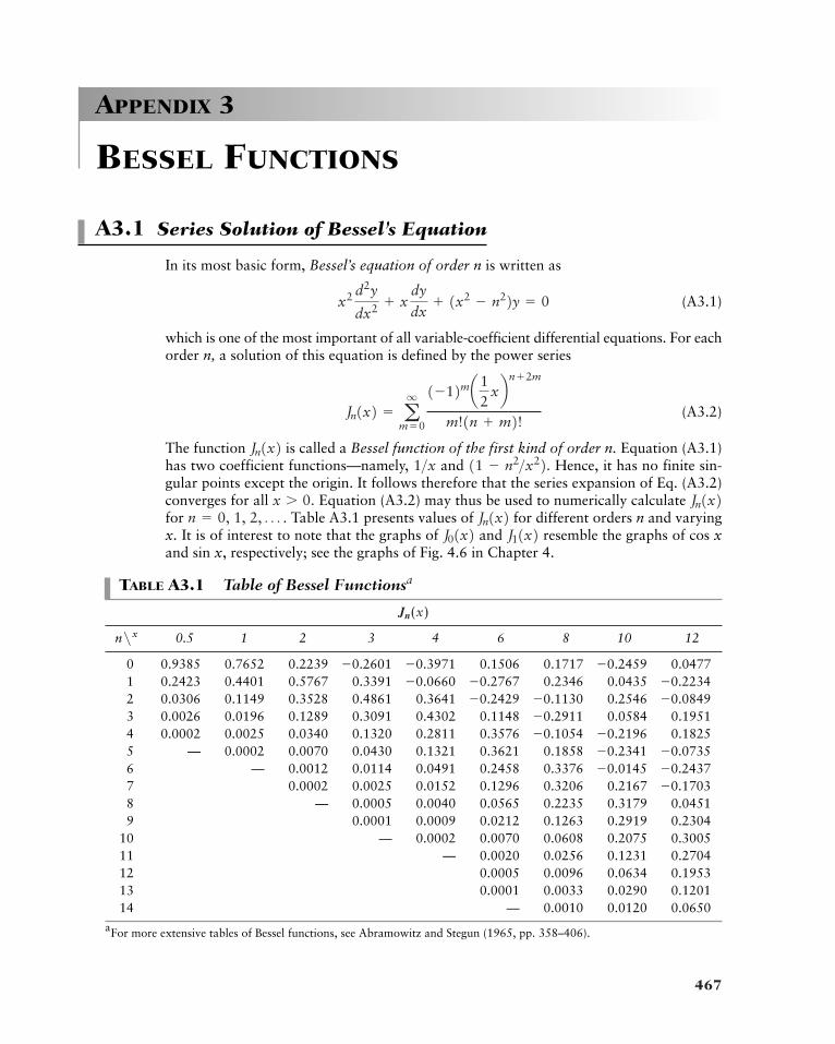
APPENDIX 3
BESSEL FUNCTIONS
A3.1 Series Solution of Bessel’s Equation
In its most basic form, Bessel’s equation of order n is written as
(A3.1)
which is one of the most important of all variable-coefficient differential equations. For eachorder n, a solution of this equation is defined by the power series
(A3.2)
The function is called a Bessel function of the first kind of order n. Equation (A3.1)has two coefficient functions—namely, and Hence, it has no finite sin-gular points except the origin. It follows therefore that the series expansion of Eq. (A3.2)converges for all Equation (A3.2) may thus be used to numerically calculate for Table A3.1 presents values of for different orders n and varyingx. It is of interest to note that the graphs of and resemble the graphs of cos xand sin x, respectively; see the graphs of Fig. 4.6 in Chapter 4.
J11x2J01x2 Jn1x2n � 0, 1, 2, Á .Jn1x2x � 0.
11 � n2>x22.1>xJn1x2Jn1x2 � a
q
m�0
1�12ma12
xbn2m
m!1n m2!
x2 d2y
dx2 xdy
dx 1x2 � n22y � 0
467
TABLE A3.1 Table of Bessel Functions
n 0.5 1 2 3 4 6 8 10 12
0 0.9385 0.7652 0.2239 0.1506 0.1717 0.04771 0.2423 0.4401 0.5767 0.3391 0.2346 0.04352 0.0306 0.1149 0.3528 0.4861 0.3641 0.25463 0.0026 0.0196 0.1289 0.3091 0.4302 0.1148 0.0584 0.19514 0.0002 0.0025 0.0340 0.1320 0.2811 0.3576 0.18255 — 0.0002 0.0070 0.0430 0.1321 0.3621 0.18586 — 0.0012 0.0114 0.0491 0.2458 0.33767 0.0002 0.0025 0.0152 0.1296 0.3206 0.21678 — 0.0005 0.0040 0.0565 0.2235 0.3179 0.04519 0.0001 0.0009 0.0212 0.1263 0.2919 0.2304
10 — 0.0002 0.0070 0.0608 0.2075 0.300511 — 0.0020 0.0256 0.1231 0.270412 0.0005 0.0096 0.0634 0.195313 0.0001 0.0033 0.0290 0.120114 — 0.0010 0.0120 0.0650
For more extensive tables of Bessel functions, see Abramowitz and Stegun (1965, pp. 358–406).a
�0.1703�0.2437�0.0145�0.0735�0.2341
�0.2196�0.1054�0.2911
�0.0849�0.1130�0.2429�0.2234�0.2767�0.0660
�0.2459�0.3971�0.2601
O x
Jn1x2
a
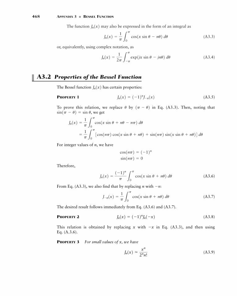
The function may also be expressed in the form of an integral as
(A3.3)
or, equivalently, using complex notation, as
(A3.4)
A3.2 Properties of the Bessel Function
The Bessel function has certain properties:
PROPERTY 1 (A3.5)
To prove this relation, we replace by in Eq. (A3.3). Then, noting thatwe get
For integer values of n, we have
Therefore,
(A3.6)
From Eq. (A3.3), we also find that by replacing n with
(A3.7)
The desired result follows immediately from Eq. (A3.6) and (A3.7).
PROPERTY 2 (A3.8)
This relation is obtained by replacing x with in Eq. (A3.3), and then using Eq. (A.3.6).
PROPERTY 3 For small values of x, we have
(A3.9)Jn1x2 Mxn
2nn!
�x
Jn1x2 � 1�12nJn1�x2
J�n1x2 �1p L
p
0 cos1x sin u nu2 du
�n:
Jn1x2 �1�12np L
p
0 cos1x sin u nu2 du
sin1np2 � 0
cos1np2 � 1�12n
�1p L
p
03cos1np2 cos1x sin u nu2 sin1np2 sin1x sin u nu24 du
Jn1x2 �1p L
p
0cos1x sin u nu � np2 du
sin1p � u2 � sin u,1p � u2u
Jn1x2 � 1�12nJ�n1x2Jn1x2
Jn1x2 �1
2p Lp
�pexp1jx sin u � jnu2 du
Jn1x2 �1p L
p
0 cos1x sin u � nu2 du
Jn1x2468 APPENDIX 3 � BESSEL FUNCTION
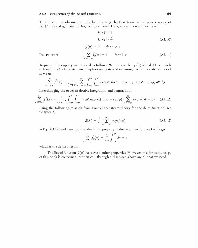
This relation is obtained simply by retaining the first term in the power series of Eq. (A3.2) and ignoring the higher order terms. Thus, when x is small, we have
(A3.10)
PROPERTY 4 (A3.11)
To prove this property, we proceed as follows. We observe that is real. Hence, mul-tiplying Eq. (A3.4) by its own complex conjugate and summing over all possible values ofn, we get
Interchanging the order of double integration and summation:
(A3.12)
Using the following relation from Fourier transform theory for the delta function (seeChapter 2)
(A3.13)
in Eq. (A3.12) and then applying the sifting property of the delta function, we finally get
which is the desired result.
The Bessel function has several other properties. However, insofar as the scopeof this book is concerned, properties 1 through 4 discussed above are all that we need.
Jn1x2
aq
n��qJn
21x2 �1
2p Lp
�pdu � 1
d1f2 �1
2p aq
n��q exp1jnf2
aq
n��qJn
21x2 �1
12p22 Lp
�pLp
�pdu df exp3jx1sin u � sin f24 aq
n��q exp3jn1f � u24
aq
n��qJn
21x2 �1
12p22 aq
n��qLp
�pLp
�p exp1jx sin u � jnu � jx sin f jnf2 du df
Jn1x2aq
n��qJn
21x2 � 1 for all x
Jn1x2 M 0 for n � 1
J11x2 Mx2
J01x2 M 1
A3.2 Properties of the Bessel Function 469
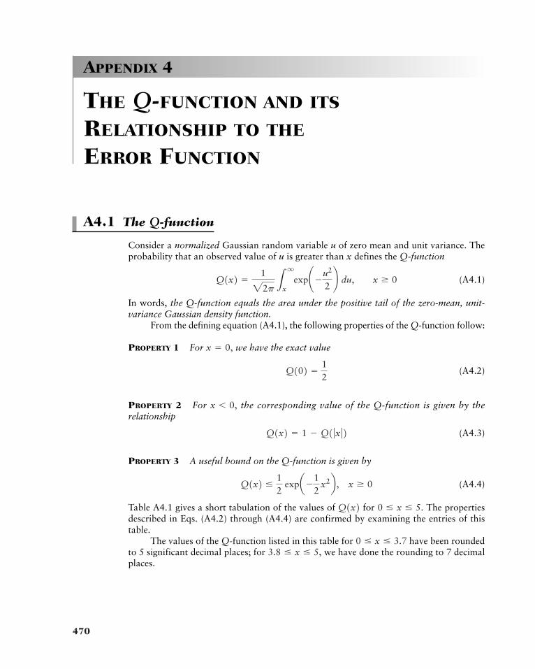
APPENDIX 4
THE Q-FUNCTION AND ITS
RELATIONSHIP TO THE
ERROR FUNCTION
A4.1 The Q-function
Consider a normalized Gaussian random variable u of zero mean and unit variance. Theprobability that an observed value of u is greater than x defines the Q-function
(A4.1)
In words, the Q-function equals the area under the positive tail of the zero-mean, unit-variance Gaussian density function.
From the defining equation (A4.1), the following properties of the Q-function follow:
PROPERTY 1 For we have the exact value
(A4.2)
PROPERTY 2 For the corresponding value of the Q-function is given by therelationship
(A4.3)
PROPERTY 3 A useful bound on the Q-function is given by
(A4.4)
Table A4.1 gives a short tabulation of the values of for The propertiesdescribed in Eqs. (A4.2) through (A4.4) are confirmed by examining the entries of thistable.
The values of the Q-function listed in this table for have been roundedto 5 significant decimal places; for we have done the rounding to 7 decimalplaces.
3.8 � x � 5,0 � x � 3.7
0 � x � 5.Q1x2Q1x2 �
12
expa�12
x2b , x � 0
Q1x2 � 1 � Q1 ƒx ƒ2x � 0,
Q102 �12
x � 0,
Q1x2 �1
22p Lq
xexp¢�
u2
2≤ du, x � 0
470
A4.2 Relationship of the Q-function tothe Complementary Error Function
The Q-function was introduced in Chapter 8 of the book and its use in evaluating theeffect of noise in digital communications was discussed in Chapter 10. In the literature, weoften find that this effect is formulated in terms of another function — namely, the com-plementary error function.
In this context, we first define the error function as
(A4.5)
The error function has two useful properties
PROPERTY 1 (A4.6)
This property is known as the symmetry relation.
PROPERTY 2 (A4.7)21p L
q
0 exp1�u22 du � 1
erf1�x2 � �erf1x2
erf1x2 �21p L
x
0 exp1�u22 du
A4.2 Relationship of the Q-function to the Complementary Error Function 471
TABLE A4.1 Table of the values of Q-function
x x
0.0 0.50000 2.2 0.013900.1 0.46017 2.3 0.010720.2 0.42074 2.4 0.008200.3 0.38209 2.5 0.006210.4 0.34458 2.6 0.004660.5 0.30854 2.7 0.003470.6 0.27425 2.8 0.002560.7 0.24196 2.9 0.001870.8 0.21186 3.0 0.001350.9 0.18406 3.1 0.000971.0 0.15866 3.2 0.000691.1 0.13567 3.3 0.000481.2 0.11507 3.4 0.000341.3 0.09680 3.5 0.000231.4 0.08076 3.6 0.000161.5 0.06681 3.7 0.000111.6 0.05480 3.81.7 0.04457 3.91.8 0.03593 4.01.9 0.02872 4.302.0 0.02275 4.652.1 0.01786 5.00
Table A4.1 is adapted from Abramowitz and Stegun (1964), pp. 966–972. Thishandbook tabulates the Gaussian (normal) probability density function
a
0.03 10�50.17 10�50.85 10�53.17 10�54.81 10�57.24 10�5
Q1x2Q1x2
a
A related function, called the complementary error function, is defined by
(A4.8)
Examining Eqs. (A4.1) and first line of Eq. (A4.8), we readily find that the Q-function andcomplementary error function as related as follows:
(A4.9)
The inverse of this relationship is given by
(A4.10)
Hence, given the Q-function, we may use Eq. (A 4.10) to calculate the corresponding valueof the complementary error function for prescribed . Conversely, given the complemen-tary error function, we may calculate the corresponding Q-function using Eq. (A4.9).
x
erfc1x2 � 2Q A22x BQ1x2 �
12
erfc¢ x
22≤
� 1 � erf1x2erfc1x2 �
2
2p Lq
x exp1�u22 du
472 APPENDIX 4 � THE Q-FUNCTION AND ITS RELATIONSHIP TO THE ERROR FUNCTION
APPENDIX 5
SCHWARZ’S INEQUALITY
Let and be functions of the real variable t in the interval We assumethat and satisfy the conditions
(A5.1)
(A5.2)
Then, according to Schwarz’s inequality, we have
(A5.3)
To prove this inequality, we first form the integral
(A5.4)
where is a real variable, the asterisk signifies complex conjugation, and
(A5.5)
(A5.6)
(A5.7)
The integral of Eq. (A5.4) exists, is real, and is a nonnegative function of say Sinceis nonnegative, it must have no real roots except possibly a double root. From the
quadratic formula, we must then have
(A5.8)
Note that is equal to the real part of B. On substituting Eqs. (A5.5) to (A5.7)into (A5.8), we get
(A5.9)
This is the most general form of Schwarz’s inequality that is appropriate for com-plex functions and For the case when both and are real, we have
(A5.10)
and Eq. (A5.3) follows immediately.
g1…1t2g21t2 g11t2g2
…1t2 � 2g11t2g21t2g21t2g11t2g21t2.g11t2
eLb
a3g1…1t2g21t2 g11t2g2
…1t24 dt f2
� 4Lb
aƒg11t2 ƒ2 dt L
b
aƒg21t2 ƒ2 dt
1B B*2>21B B*22 � 4AC
f1l2 f1l2.l,
C � Lb
aƒg21t2 ƒ2 dt � 0
B � Lb
ag1…1t2g21t2 dt
A � Lb
aƒg11t2 ƒ2 dt � 0
l
Lb
a3lg1…1t2 g2
…1t243lg11t2 g21t24 dt � l2A l1B B…2 C
` Lb
ag11t2g21t2 dt ` 2 � L
b
aƒg11t2 ƒ2 dt L
b
aƒg21t2 ƒ2 dt
Lb
aƒg21t2 ƒ2 dt � �
Lb
aƒg11t2 ƒ2 dt � �
g21t2g11t2 a � t � b.g21t2g11t2
473
Note that equality is obtained [aside from the trivial case where both and are zero] when the double root exists in Eq. (A5.4); that is, when
(A5.11)
Since is real, and are linearly related. Looking at the problem from a slightlydifferent viewpoint, we see that there is a real value of for which Eq. (A5.4) is zero andfor which its first derivative with respect to vanishes; that is.
(A5.12)
or
(A5.13)
This relation holds if, and only if,
(A5.14)
This last relationship is equivalent to Eq. (A5.11).
g21t2 � �lg11t2
l � �B B…
2A� �
Lb
a3g1…1t2g21t2 g11t2g2
…1t24 dt
2Lb
aƒg11t2 ƒ2 dt
2lA 1B B…2 � 0
l
l
g21t2g11t2l
lg11t2 g21t2 � lg1…1t2 g2
…1t2 � 0
g21t2g11t2474 APPENDIX 5 � SCHWARZ’S INEQUALITY
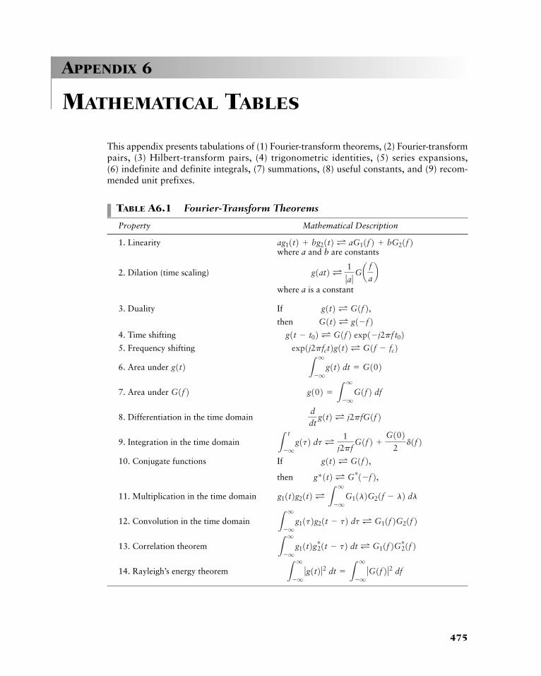
APPENDIX 6
MATHEMATICAL TABLES
This appendix presents tabulations of (1) Fourier-transform theorems, (2) Fourier-transformpairs, (3) Hilbert-transform pairs, (4) trigonometric identities, (5) series expansions,(6) indefinite and definite integrals, (7) summations, (8) useful constants, and (9) recom-mended unit prefixes.
475
TABLE A6.1 Fourier-Transform Theorems
Property Mathematical Description
1. Linearitywhere a and b are constants
2. Dilation (time scaling)
where a is a constant
3. Duality If
then
4. Time shifting
5. Frequency shifting
6. Area under
7. Area under
8. Differentiation in the time domain
9. Integration in the time domain
10. Conjugate functions If
then
11. Multiplication in the time domain
12. Convolution in the time domain
13. Correlation theorem
14. Rayleigh’s energy theorem Lq
�qƒg1t2 ƒ2 dt � L
q
�qƒG1f2 ƒ2 df
Lq
�qg11t2g2
…1t � t2 dt L G11f2G2…1f2
Lq
�qg11t2g21t � t2 dt L G11f2G21f2
g11t2g21t2 L Lq
�qG11l2G21f � l2 dl
g*1t2 L G…1�f2,g1t2 L G1f2,L
t
�qg1t2 dt L 1
j2pfG1f2
G1022d1f2
ddt
g1t2 L j2pfG1f2g102 � L
q
�qG1f2 dfG1f2
Lq
�qg1t2 dt � G102g1t2
exp1j2pfct2g1t2 L G1f � fc2g1t � t02 L G1f2 exp1�j2pf t02
G1t2 L g1�f2g1t2 L G1f2,
g1at2 L 1
ƒa ƒGa f
ab
ag11t2 bg21t2 L aG11f2 bG21f2
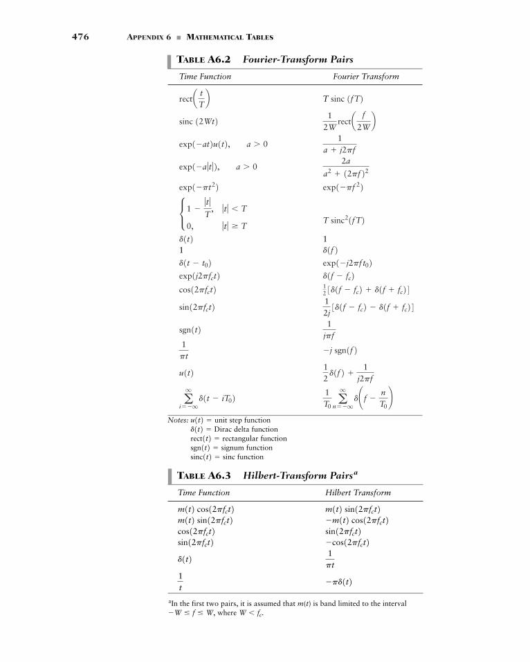
476 APPENDIX 6 � MATHEMATICAL TABLES
TABLE A6.2 Fourier-Transform Pairs
Time Function Fourier Transform
T
11
Notes: step functiondelta function
functionfunction
functionsinc1t2 � sincsgn1t2 � signumrect1t2 � rectangulard1t2 � Diracu1t2 � unit
1T0aq
n��qd¢f �
nT0≤a
q
i��qd1t � iT02
12d1f2
1j2pf
u1t2�j sgn1f21
pt
1jpf
sgn1t212j3d1f � fc2 � d1f fc24sin12pfct2
12 3d1f � fc2 d1f fc24cos12pfct2d1f � fc2exp1j2pfct2exp1�j2pf t02d1t � t02d1f2d1t2T sinc21fT2c 1 �
ƒt ƒT
, ƒt ƒ � T
0, ƒt ƒ � T
exp1�pf 22exp1�pt222a
a2 12pf22exp1�a ƒt ƒ2, a � 0
1a j2pf
exp1�at2u1t2, a � 0
12W
recta f
2Wbsinc 12Wt2
sinc 1fT2recta tTb
TABLE A6.3 Hilbert-Transform Pairsa
Time Function Hilbert Transform
aIn the first two pairs, it is assumed that m(t) is band limited to the intervalwhere W � fc.�W � f � W,
�pd1t21t
1pt
d1t2�cos12pfct2sin12pfct2sin12pfct2cos12pfct2�m1t2 cos12pfct2m1t2 sin12pfct2m1t2 sin12pfct2m1t2 cos12pfct2
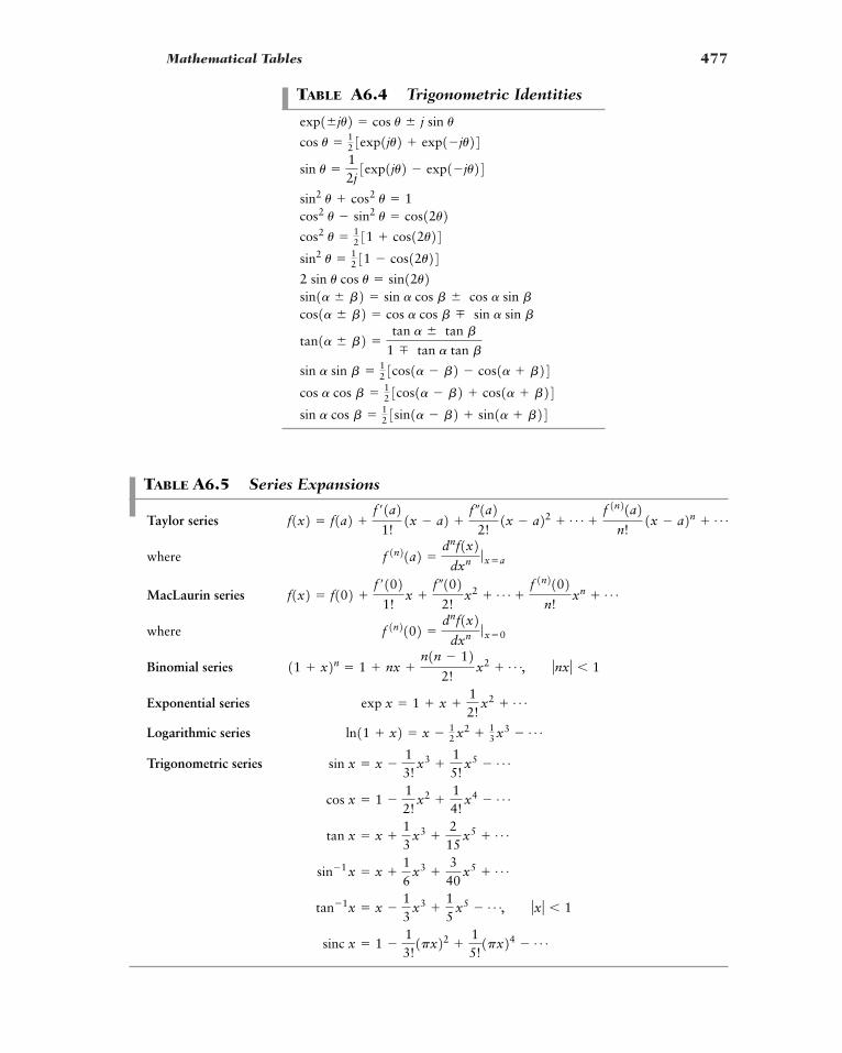
Mathematical Tables 477
TABLE A6.4 Trigonometric Identities
sin a cos b � 12 3sin1a � b2 sin1a b24
cos a cos b � 12 3cos1a � b2 cos1a b24
sin a sin b � 12 3cos1a � b2 � cos1a b24
tan1a � b2 �tan a � tan b
1 < tan a tan b
cos1a � b2 � cos a cos b < sin a sin bsin1a � b2 � sin a cos b � cos a sin b2 sin u cos u � sin12u2sin2 u � 1
2 31 � cos12u24cos2 u � 1
2 31 cos12u24cos2 u � sin2 u � cos12u2sin2 u cos2 u � 1
sin u �12j3exp1ju2 � exp1�ju24
cos u � 12 3exp1ju2 exp1�ju24
exp1�ju2 � cos u � j sin u
TABLE A6.5 Series Expansions
Taylor series
where
MacLaurin series
where
Binomial series
Exponential series
Logarithmic series
Trigonometric series
sinc x � 1 �13!1px22
15!1px24 � Á
tan�1x � x �13
x3 15
x5 � Á, ƒx ƒ � 1
sin�1 x � x 16
x3 340
x5 Á
tan x � x 13
x3 215
x5 Á
cos x � 1 �12!
x2 14!
x4 � Á
sin x � x �13!
x3 15!
x5 � Á
ln11 x2 � x � 12 x2 1
3 x3 � Á
exp x � 1 x 12!
x2 Á
11 x2n � 1 nx n1n � 12
2!x2 Á, ƒnx ƒ � 1
f 1n2102 �dnf1x2
dxn ƒ x�0
f1x2 � f102 f �102
1!x
f �1022!
x2 Á f 1n2102
n!xn Á
f 1n21a2 �dnf1x2
dxn ƒ x�a
f1x2 � f1a2 f �1a2
1!1x � a2
f �1a22!1x � a22 Á
f 1n21a2n!
1x � a2n Á
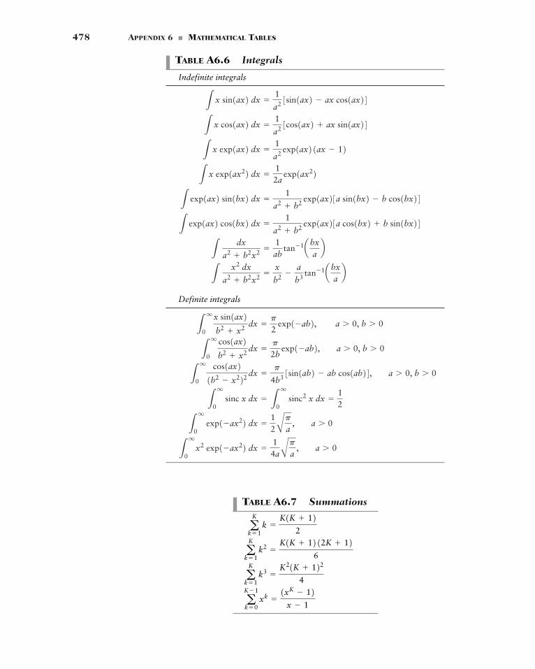
478 APPENDIX 6 � MATHEMATICAL TABLES
TABLE A6.6 Integrals
Indefinite integrals
Definite integrals
Lq
0x2 exp1�ax22 dx �
14aApa , a � 0
Lq
0 exp1�ax22 dx �
12Apa , a � 0
Lq
0 sinc x dx � L
q
0 sinc2 x dx �
12
Lq
0
cos1ax21b2 � x222 dx �
p
4b3 3sin1ab2 � ab cos1ab24, a � 0, b � 0
Lq
0
cos1ax2b2 x2 dx �
p
2bexp1�ab2, a � 0, b � 0
Lq
0
x sin1ax2b2 x2 dx �
p
2exp1�ab2, a � 0, b � 0
Lx2 dx
a2 b2x2 �x
b2 �a
b3 tan�1abxab
Ldx
a2 b2x2 �1ab
tan�1abxab
L exp1ax2 cos1bx2 dx �1
a2 b2 exp1ax23a cos1bx2 b sin1bx24L exp1ax2 sin1bx2 dx �
1
a2 b2 exp1ax23a sin1bx2 � b cos1bx24Lx exp1ax22 dx �
12a
exp1ax22Lx exp1ax2 dx �
1
a2 exp1ax21ax � 12Lx cos1ax2 dx �
1
a2 3cos1ax2 ax sin1ax24Lx sin1ax2 dx �
1
a2 3sin1ax2 � ax cos1ax24
TABLE A6.7 Summations
aK�1
k�0xk �
1xK � 12x � 1
aK
k�1k3 �
K21K 1224
aK
k�1k2 �
K1K 1212K 126
aK
k�1k �
K1K 122
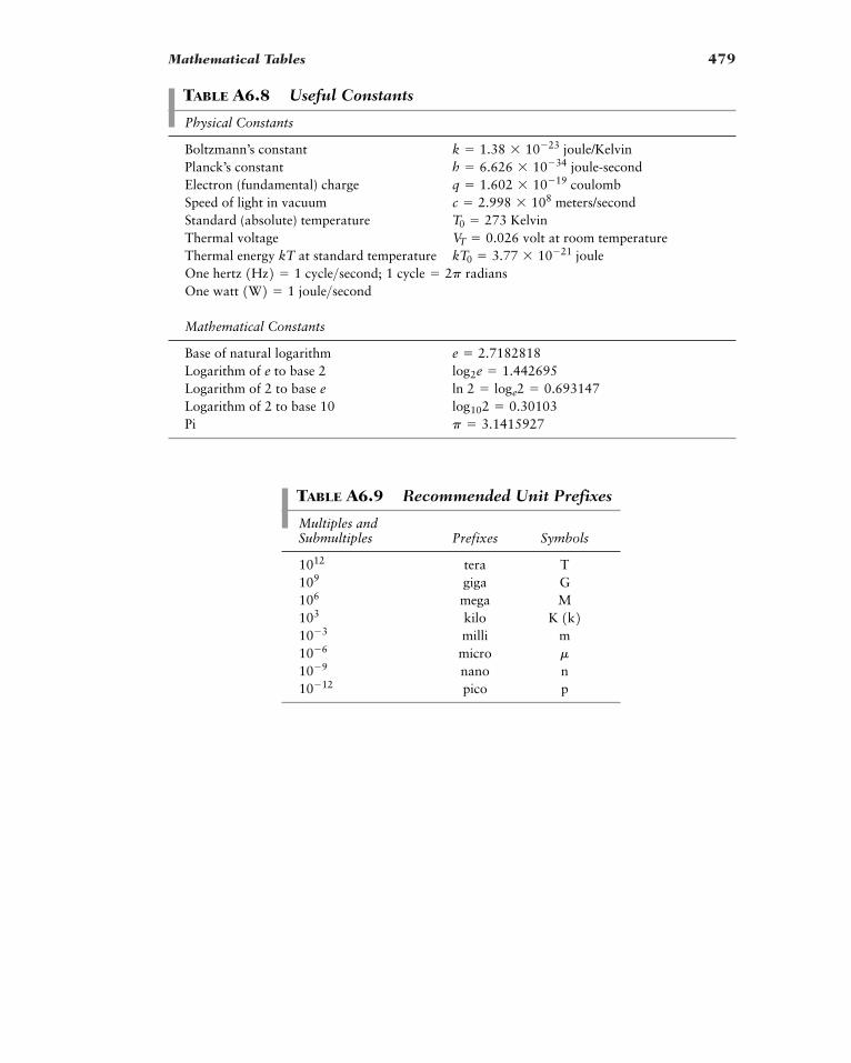
Mathematical Tables 479
TABLE A6.8 Useful Constants
Physical Constants
Boltzmann’s constant joule/KelvinPlanck’s constant joule-secondElectron (fundamental) charge coulombSpeed of light in vacuum meters/secondStandard (absolute) temperature KelvinThermal voltage volt at room temperatureThermal energy kT at standard temperature jouleOne hertz One watt
Mathematical Constants
Base of natural logarithmLogarithm of e to base 2Logarithm of 2 to base eLogarithm of 2 to base 10Pi p � 3.1415927
log102 � 0.30103ln 2 � loge2 � 0.693147log2e � 1.442695e � 2.7182818
1W2 � 1 joule>second1 cycle � 2p radians1Hz2 � 1 cycle>second;
kT0 � 3.77 10�21VT � 0.026T0 � 273c � 2.998 108q � 1.602 10�19h � 6.626 10�34k � 1.38 10�23
TABLE A6.9 Recommended Unit Prefixes
Multiples and Submultiples Prefixes Symbols
tera Tgiga Gmega Mkilomilli mmicronano npico p10�12
10�9m10�6
10�3K 1k2103
1061091012
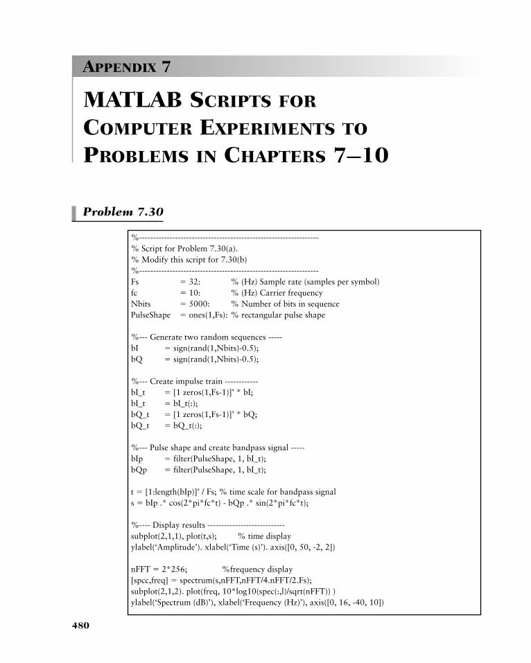
APPENDIX 7
MATLAB SCRIPTS FOR
COMPUTER EXPERIMENTS TO
PROBLEMS IN CHAPTERS 7–10
Problem 7.30
480
%-----------------------------------------------------------------% Script for Problem 7.30(a).% Modify this script for 7.30(b)%-----------------------------------------------------------------Fs � 32: % (Hz) Sample rate (samples per symbol)fc � 10: % (Hz) Carrier frequencyNbits � 5000: % Number of bits in sequencePulseShape � ones(1,Fs): % rectangular pulse shape
%--- Generate two random sequences -----bI � sign(rand(1,Nbits)-0.5);bQ � sign(rand(1,Nbits)-0.5);
%--- Create impulse train ------------bI_t � [1 zeros(1,Fs-1)]’ * bI;bI_t � bI_t(:);bQ_t � [1 zeros(1,Fs-1)]’ * bQ;bQ_t � bQ_t(:);
%--- Pulse shape and create bandpass signal -----bIp � filter(PulseShape, 1, bI_t);bQp � filter(PulseShape, 1, bI_t);
t � [1:length(bIp)]’ / Fs; % time scale for bandpass signal s � bIp .* cos(2*pi*fc*t) - bQp .* sin(2*pi*fc*t);
%---- Display results ----------------------------subplot(2,1,1), plot(t,s); % time displayylabel(‘Amplitude’). xlabel(‘Time (s)’). axis([0, 50, -2, 2])
nFFT � 2*256; %frequency display[spcc,freq] � spectrum(s,nFFT,nFFT/4.nFFT/2.Fs);subplot(2,1,2). plot(freq, 10*log10(spec(:,l)/sqrt(nFFT)) )ylabel(‘Spectrum (dB)’), xlabel(‘Frequency (Hz)’), axis([0, 16, -40, 10])
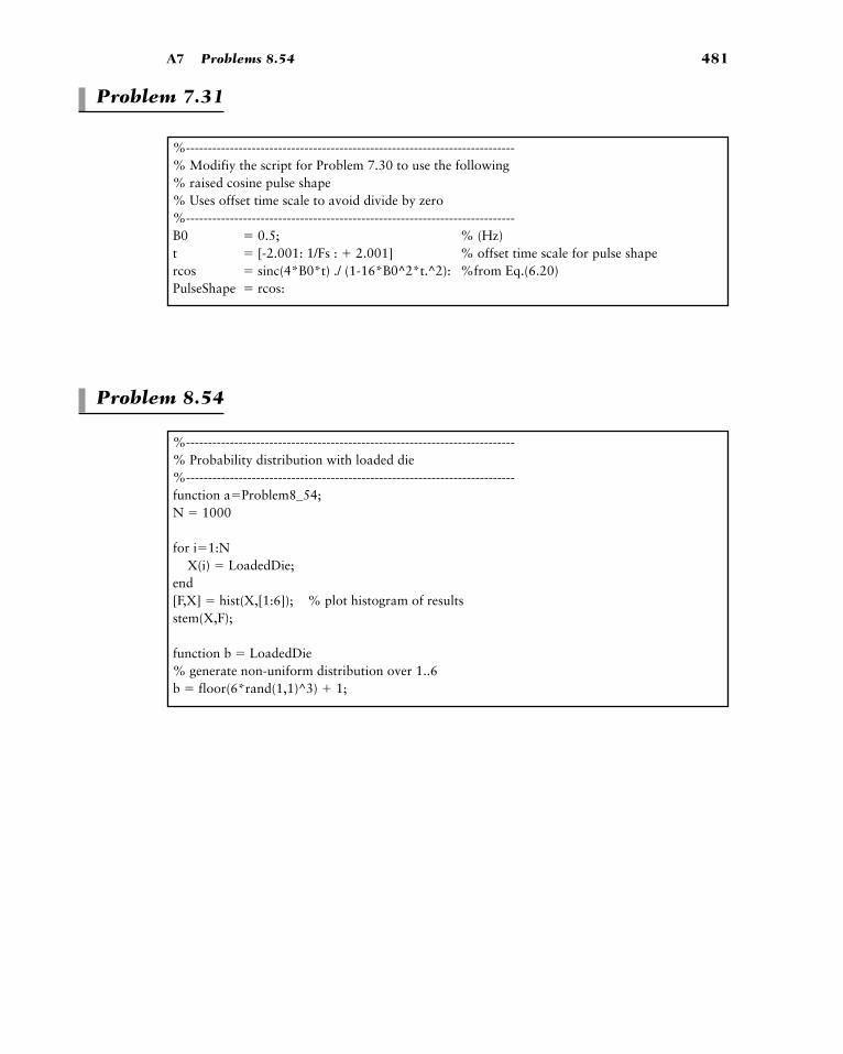
Problem 7.31
A7 Problems 8.54 481
%---------------------------------------------------------------------------% Modifiy the script for Problem 7.30 to use the following% raised cosine pulse shape% Uses offset time scale to avoid divide by zero%---------------------------------------------------------------------------B0 � 0.5; % (Hz)t � [-2.001: 1/Fs : 2.001] % offset time scale for pulse shapercos � sinc(4*B0*t) ./ (1-16*B0^2*t.^2): %from Eq.(6.20)PulseShape � rcos:
Problem 8.54
%---------------------------------------------------------------------------% Probability distribution with loaded die%---------------------------------------------------------------------------function a�Problem8_54;N � 1000
for i�1:NX(i) � LoadedDie;
end[F,X] � hist(X,[1:6]); % plot histogram of resultsstem(X,F);
function b � LoadedDie% generate non-uniform distribution over 1..6b � floor(6*rand(1,1)^3) 1;
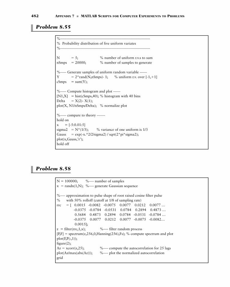
Problem 8.58
482 APPENDIX 7 � MATLAB SCRIPTS FOR COMPUTER EXPERIMENTS TO PROBLEMS
%---------------------------------------------------------------------------% Probability distribution of five uniform variates%---------------------------------------------------------------------------
N � 5; % number of uniform r.v.s to sumnSmps � 20000; % number of samples to generate
%----- Generate samples of uniform random variable ------Y � 2*rand(N,nSmps)- 1; % uniform r.v. over [-1,1]cSmps � sum(Y);
%----- Compute histogram and plot ------[N1,X] � hist(cSmps,40); % histogram with 40 binsDelta � X(2)- X(1);plot(X, N1/nSmps/Delta); % normalize plot
%----- compare to theory -------hold onx � [-5:0.01:5]sigma2 � N*(1/3); % variance of one uniform is 1/3Gauss � exp(-x.^2/2/sigma2) / sqrt(2*pi*sigma2);plot(x,Gauss,’r’);hold off
Problem 8.55
N � 100000; %---- number of samplesx � randn(1,N); %---- generate Gaussian sequence
%---- approximation to pulse shape of root raised cosine filter pulse% with 50% rolloff (cutoff at 1/8 of sampling rate)rrc � [ 0.0015 -0.0082 -0.0075 0.0077 0.0212 0.0077 …
-0.0375 -0.0784 -0.0531 0.0784 0.2894 0.4873 …0.5684 0.4873 0.2894 0.0784 -0.0531 -0.0784 …-0.0375 0.0077 0.0212 0.0077 -0.0075 -0.0082…0.0015];
z � filter(rrc,1,x); %---- filter random process[P,F] � spectrum(z,256,0,Hanning(256),Fs); % compute spectrum and plotplot(F,P(:,1));figure(2);Az � xcorr(z,25); %---- compute the autocorrelation for 25 lagsplot(Az/max(abs(Az))); %---- plot the normalized autocorrelationgrid
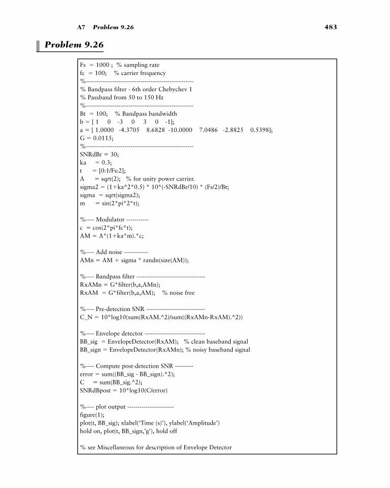
Problem 9.26
A7 Problem 9.26 483
Fs � 1000 ; % sampling ratefc � 100; % carrier frequency%-----------------------------------------------------% Bandpass filter - 6th order Chebychev 1% Passband from 50 to 150 Hz%-----------------------------------------------------Bt � 100; % Bandpass bandwidthb � [ 1 0 -3 0 3 0 -1];a � [ 1.0000 -4.3705 8.6828 -10.0000 7.0486 -2.8825 0.5398];G � 0.0115;%-----------------------------------------------------SNRdBr � 30;ka � 0.3;t � [0:1/Fs:2];A � sqrt(2); % for unity power carrier.sigma2 � (1ka^2*0.5) * 10^(-SNRdBr/10) * (Fs/2)/Bt;sigma � sqrt(sigma2);m � sin(2*pi*2*t);
%---- Modulator -----------c � cos(2*pi*fc*t);AM � A*(1ka*m).*c;
%---- Add noise ------------AMn � AM sigma * randn(size(AM));
%---- Bandpass filter ----------------------------------RxAMn � G*filter(b,a,AMn);RxAM � G*filter(b,a,AM); % noise free
%---- Pre-detection SNR -----------------------------C_N � 10*log10(sum(RxAM.^2)/sum((RxAMn-RxAM).^2))
%---- Envelope detector ------------------------------BB_sig � EnvelopeDetector(RxAM); % clean baseband signalBB_sign � EnvelopeDetector(RxAMn); % noisy baseband signal
%---- Compute post-detection SNR ---------error � sum((BB_sig - BB_sign).^2);C � sum(BB_sig.^2);SNRdBpost � 10*log10(C/error)
%---- plot output -----------------------figure(1);plot(t, BB_sig); xlabel(‘Time (s)’), ylabel(‘Amplitude’)hold on, plot(t, BB_sign,’g’), hold off
% see Miscellaneous for description of Envelope Detector
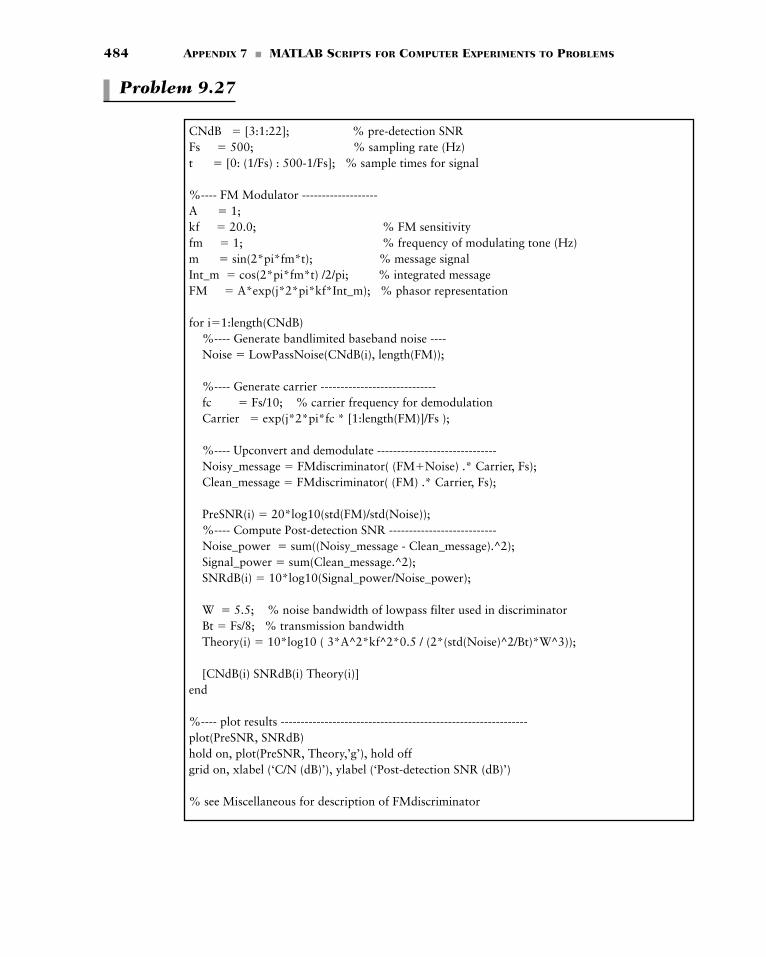
Problem 9.27
484 APPENDIX 7 � MATLAB SCRIPTS FOR COMPUTER EXPERIMENTS TO PROBLEMS
CNdB � [3:1:22]; % pre-detection SNRFs � 500; % sampling rate (Hz)t � [0: (1/Fs) : 500-1/Fs]; % sample times for signal
%---- FM Modulator -------------------A � 1;kf � 20.0; % FM sensitivityfm � 1; % frequency of modulating tone (Hz)m � sin(2*pi*fm*t); % message signalInt_m � cos(2*pi*fm*t) /2/pi; % integrated messageFM � A*exp(j*2*pi*kf*Int_m); % phasor representation
for i�1:length(CNdB)%---- Generate bandlimited baseband noise ---- Noise � LowPassNoise(CNdB(i), length(FM));
%---- Generate carrier -----------------------------fc � Fs/10; % carrier frequency for demodulationCarrier � exp(j*2*pi*fc * [1:length(FM)]/Fs );
%---- Upconvert and demodulate ------------------------------Noisy_message � FMdiscriminator( (FMNoise) .* Carrier, Fs);Clean_message � FMdiscriminator( (FM) .* Carrier, Fs);
PreSNR(i) � 20*log10(std(FM)/std(Noise));%---- Compute Post-detection SNR ---------------------------Noise_power � sum((Noisy_message - Clean_message).^2);Signal_power � sum(Clean_message.^2);SNRdB(i) � 10*log10(Signal_power/Noise_power);
W � 5.5; % noise bandwidth of lowpass filter used in discriminatorBt � Fs/8; % transmission bandwidthTheory(i) � 10*log10 ( 3*A^2*kf^2*0.5 / (2*(std(Noise)^2/Bt)*W^3));
[CNdB(i) SNRdB(i) Theory(i)]end
%---- plot results --------------------------------------------------------------plot(PreSNR, SNRdB)hold on, plot(PreSNR, Theory,’g’), hold offgrid on, xlabel (‘C/N (dB)’), ylabel (‘Post-detection SNR (dB)’)
% see Miscellaneous for description of FMdiscriminator
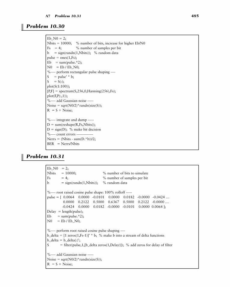
Problem 10.30
A7 Problem 10.31 485
Eb_N0 � 2;Nbits � 10000; % number of bits, increase for higher Eb/N0Fs � 4; % number of samples per bitb � sign(randn(1,Nbits)); % random datapulse � ones(1,Fs);Eb � sum(pulse.^2);N0 � Eb / Eb_N0;%---- perform rectangular pulse shaping ----S � pulse’ * b;S � S(:);plot(S(1:100));[P,F] � spectrum(S,256,0,Hanning(256),Fs);plot(F,P(:,1));%---- add Gaussian noise -----Noise � sqrt(N0/2)*randn(size(S));R � S Noise;
%---- integrate and dump -----D � sum(reshape(R,Fs,Nbits));D � sign(D); % make bit decision%---- count errors --------------Nerrs � (Nbits - sum(D.*b))/2;BER � Nerrs/Nbits
Problem 10.31
Eb_N0 � 2;Nbits � 10000; % number of bits to simulate Fs � 4; % number of samples per bitb � sign(randn(1,Nbits)); % random data
%---- root raised cosine pulse shape: 100% rolloff -----pulse � [ 0.0064 0.0000 -0.0101 0.0000 0.0182 -0.0000 -0.0424 …
0.0000 0.2122 0.5000 0.6367 0.5000 0.2122 -0.0000 …-0.0424 0.0000 0.0182 -0.0000 -0.0101 0.0000 0.0064 ];
Delay � length(pulse);Eb � sum(pulse.^2);N0 � Eb / Eb_N0;
%---- perform root raised cosine pulse shaping ----b_delta � [1 zeros(1,Fs-1)]’ * b; % make b into a stream of delta functionsb_delta � b_delta(:)’;S � filter(pulse,1,[b_delta zeros(1,Delay)]); % add zeros for delay of filter
%---- add Gaussian noise -----Noise � sqrt(N0/2)*randn(size(S));R � S Noise;
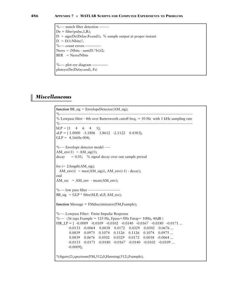
Miscellaneous
486 APPENDIX 7 � MATLAB SCRIPTS FOR COMPUTER EXPERIMENTS TO PROBLEMS
%---- match filter detection --------De � filter(pulse,1,R);D � sign(De(Delay:Fs:end)); % sample output at proper instantD � D(1:Nbits)’;%---- count errors -------------Nerrs � (Nbits - sum(D.*b))/2;BER � Nerrs/Nbits
%---- plot eye diagram -------------ploteye(De(Delay:end), Fs)
function BB_sig � EnvelopeDetector(AM_sig);%----------------------------------------------------------------------------------------------------------------% Lowpass filter - 4th over Butterworth cutoff freq. � 50 Hz with 1 kHz sampling rate%----------------------------------------------------------------------------------------------------------------bLP � [1 4 6 4 1];aLP � [ 1.0000 -3.1806 3.8612 -2.1122 0.4383];GLP � 4.1660e-004;
%---- Envelope detector model -----AM_env(1) � AM_sig(1);decay � 0.01; % signal decay over one sample period
for i� 2:length(AM_sig);AM_env(i) � max(AM_sig(i), AM_env(i-1) - decay);
endAM_rec � AM_env - mean(AM_env);
%---- low pass filter ---------------------------BB_sig � GLP * filter(bLP, aLP, AM_rec);
function Message � FMdiscriminator(FM,Fsample);
%---- Lowpass Filter: Finite Impulse Response %---- (36 taps Fsample � 125 Hz, Fpass�5Hz Fstop� 10Hz, 40dB )FIR_LP � [ -0.0009 -0.0109 -0.0102 -0.0140 -0.0167 -0.0180 -0.0171 ...
-0.0133 -0.0064 0.0038 0.0172 0.0329 0.0502 0.0676 ...0.0839 0.0975 0.1074 0.1126 0.1126 0.1074 0.0975 ...0.0839 0.0676 0.0502 0.0329 0.0172 0.0038 -0.0064 ...-0.0133 -0.0171 -0.0180 -0.0167 -0.0140 -0.0102 -0.0109 ...-0.0009];
%figure(2),spectrum(FM,512,0,Hanning(512),Fsample);
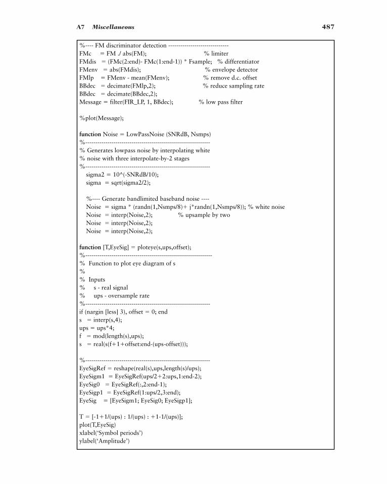
A7 Miscellaneous 487
%---- FM discriminator detection ------------------------------FMc � FM ./ abs(FM); % limiterFMdis � (FMc(2:end)- FMc(1:end-1)) * Fsample; % differentiatorFMenv � abs(FMdis); % envelope detectorFMlp � FMenv - mean(FMenv); % remove d.c. offsetBBdec � decimate(FMlp,2); % reduce sampling rateBBdec � decimate(BBdec,2);Message � filter(FIR_LP, 1, BBdec); % low pass filter
%plot(Message);
function Noise � LowPassNoise (SNRdB, Nsmps)%--------------------------------------------------------------% Generates lowpass noise by interpolating white% noise with three interpolate-by-2 stages%--------------------------------------------------------------
sigma2 � 10^(-SNRdB/10);sigma � sqrt(sigma2/2);
%---- Generate bandlimited baseband noise ---- Noise � sigma * (randn(1,Nsmps/8) j*randn(1,Nsmps/8)); % white noiseNoise � interp(Noise,2); % upsample by twoNoise � interp(Noise,2);Noise � interp(Noise,2);
function [T,EyeSig] � ploteye(s,ups,offset);%---------------------------------------------------------------% Function to plot eye diagram of s%% Inputs% s - real signal% ups - oversample rate%--------------------------------------------------------------if (nargin [less] 3), offset � 0; ends � interp(s,4);ups � ups*4;f � mod(length(s),ups);s � real(s(f1offset:end-(ups-offset)));
%--------------------------------------------------------------EyeSigRef � reshape(real(s),ups,length(s)/ups);EyeSigm1 � EyeSigRef(ups/22:ups,1:end-2);EyeSig0 � EyeSigRef(:,2:end-1);EyeSigp1 � EyeSigRef(1:ups/2,3:end);EyeSig � [EyeSigm1; EyeSig0; EyeSigp1];
T � [-11/(ups) : 1/(ups) : 1-1/(ups)];plot(T,EyeSig)xlabel(‘Symbol periods’)ylabel(‘Amplitude’)
488
APPENDIX 8
ANSWERS TO DRILL
PROBLEMS
Notes:
1. Chapter 1 has no Drill Problems and therefore no answers.2. Many of the Drill Problems in Chapters 2 through 11 have the answers embodied in
the problem statements; hence, these problems are not addressed here.
Chapter 2
2.1
2.2
2.3 The imaginary part of must be zero.2.4 The imaginary part of must be an odd function of
2.11
2.12 (a) It is possible for a system to be causal but unstable.(b) By the same token, it is possible for the system to be stable but noncausal.
2.13
2.14 (a)
(b)
The implication of this result is a constant delay in signal transmission across the
filter, hence no phase distortion.(c) The time delay is equal to .
2.15
2.16
2.17 Eg1f2 �4a2
1a2 4p2f 222 , �� � f � �
Eg1f2 �1
a2 4p2f 2 , �� � f � �
Ryx… 1�t2 � Rxy1t2
1N � 12¢t>2
arg1H1f22 � expa�j2paN � 12bf¢tb
ƒH1f2 ƒ � wN�12
2 a121N�12�1
n�0wn cos12pnf ¢t2
H1f2 � 22pt exp1�2p2t2f 22
1 T aq
m�1 cos12pmf0t2 � T0 a
q
n��qd1f � nf02, f0 � 1>T0
f.G1f2G102g1t2 �
1pt1e�j2pWt � 12
G1f2 �2pfc
1 4p21f � fc22
A8 Answers to Drill Problems 489
Chapter 3
3.1 The envelope of the AM signal can assume zero value, if for some t,where is the amplitude sensitivity factor and is the message signal.
3.2 (a) 98%(b) 1%
3.3 where is the carrier frequency and W is the message bandwidth.3.4 (a) The spectral context of the output consists of two parts:
AM part:
Undesirable part:
(b) The required band-pass filter must have bandwidth 2W centered on that is,the cutoff frequencies of the filter are and
(c) To extract the AM wave, we require 3.5 The average power in the lower or upper side-frequency, expressed as a percentage
of the average power in the DSB-SC modulated wave, is 50%.
3.6 (a)
(b) The two sinusoidal terms inside the first set of square brackets are produced bythe upper side-frequency at The other two sinusoidal terms inside thesecond set of square brackets are produced by the side-frequency at
3.7 Spectral overlap occurs when When this happens, part of the lower sidebandmoves into the negative frequency region, and the corresponding part of the imageof that sideband moves into the positive frequency region, causing spectral overlap.The coherent detection then breaks down because the detector is unable to resolve partof the spectrum where overlap occurs.
3.12 For the coherent detector to recover the original message signal (except for scaling),we require that
Chapter 4
4.2 The phase sensitivity factor is measured in radians/volt. The frequency sensitivityfactor is measured in hertz/volt. Therefore, the dimensionality of product term
is
which is the same as the dimensionality of kp .
� radians>volt
1hertz/volt2 1second2 � a cycles
second1
voltb 1second2
2pkfTkf
kp
fc � W.
fc � W.fc � fm .
fc fm .
14
AcAm3cos12p12fc � fm2t2 cos12pfmt24v1t2 �
14
AcAm3cos12p12fc fm2t2 cos12pfmt24
fc � 3W.fc W.fc � W
fc ;F3a1m1t2 a2Ac
2 cos212pfct2 a2m21t24
F31a1 2a2m1t22cos12pfct24 �12
a11d1f � fc2 d1f fc22 a21M1f � fc2 M1f fc22
v21t2fcfc � W,
m1t2ka
kam1t2 � �1
490 APPENDIX 8 � ANSWERS TO DRILL PROBLEMS
4.4 (a) The envelope is
Maximum envelope occurs when thereby attaining the value
Minimum envelope occurs when thereby attaining the value Therefore,
(b)
(c) The harmonic distortion is produced by the term For
radian, the distortion is which is small enough to be ignored.
Chapter 5
5.5 (a)(b)(c) Nyquist rate and Nyquist interval are the same as in part (b).
5.6 (a) For
(b) For
(c) For
5.7 The Nyquist rate must exceed 1 Hz; correspondingly, the Nyquist interval must beless than 1s.
gd1t2 � aq
n��q cos11.5np2d1t � 1.5n2.
Ts � 1.5s,
gd1t2 � aq
n��q1�12nd1t � n2.
Ts � 1s,
gd1t2 � aq
n��q cosanp
4bd1t � 0.25n2.
Ts � 0.25s,
Nyquist rate � 400 Hz; Nyquist interval � 2.5 ms.Nyquist rate � 200 Hz; Nyquist interval � 5 ms.
9 10�3 � 1%,
b � 0.3b3
3 sin312pfmt2.
Average power of narrow-band FM
Average power of unmodulated carrier� a1
12b2b
1Envelope2max1Envelope2min� 1
12b2
Ac .sin12pfmt2 � 0,
Aca1 12b2b .
sin12pfmt2 � �1,
� Ac¢1 14b2 �
b2
4 sin14pfmt2≤� Aca1
12b2 sin212pfmt2b for small b.
a1t2 � Ac31 b2 sin212pfmt2
A8 Answers to Drill Problems 491
Chapter 6
6.1 For the input 001101001, the waveform at the receiver output consists of whenever symbol 1 is transmitted and whenever symbol 0 is transmit-ted. There will be no intersymbol interference because the sinc pulse goes through zerowhenever another symbol is transmitted.
6.4 (b) The value assigned to the delay should decrease with increasing (i) for (ii) for (iii) for
Chapter 7
7.6 Starting at zero, the trellis increases linearly reaching radians on the transmissionof 11, then decreases linearly to on the transmission of 0, increases to on thetransmission of 1; the level is equal to modulo . It then increases linearly from
to on the transmission of 111. Finally, it decreases linearly to on thetransmission of 00.
7.8 The linear input-output characteristic of the frequency discriminator has the follow-ing specifications:
� It occupies the frequency range
� It goes through zero at
Chapter 8
8.1 0.82
8.2
8.3
8.4 (a) 0.5(b) 0.5(c) 0.9999(d) 0.0001
8.5 and
8.6 0 and 1
1b � a22>121b a2>2
pp0
pp0 11 � p2p1 and
pp1
pp1 11 � p2p0
5.5 10�5
f � fc .
fc �14
Tb � f � fc 14
Tb .
�p>2p>2�p2p�pp
pp>2 p
a � 1t � 2.5sa � 1>2t � 3sa � 0t � 5s
a:t
�sinc1t>Tb2 sinc1t>Tb2
492 APPENDIX 8 � ANSWERS TO DRILL PROBLEMS
8.7
8.10 0 and 5/3.
8.11 Yes
8.13 ; No.
8.14 Yes
8.15 and corresponds to frequency where is
the sampling rate, where
8.16 Yes
8.17 (a)
(b)
Chapter 9
9.1 where ( ) indicates independent power measurements.
9.2 18 dB9.3 is 0.04 and 0.14.9.4 Envelope detection is insensitive to a phase offset.9.5 18 dB and the SSB transmission bandwidth is half that of DSB-SC.9.6 8 kHz and 20.1 dB9.7 Upper channel is worse by 17.1 dBs9.8 34.7 dB and 48.3 dB
SNRAMPOST>SNRDSB
POST
SNR �1S N2 � 1N2
1N2
SY1k2 � N0 ` 1 � 1aWk2N1 � aWk ` 2
N0
b0 � 1a02
a122s2 and b1 � a0a1s
2.
fskfsN
SY1k2SY1k2 � b0 2b1 cosa2pkNb
RY1n2 � 1a02
a122s2d1n2 a0a1s
21d1n � 12 d1n 122;RX1t1, t22 � 16 Ccos12pf1t1 � t222 cos12pf1t1 t222 D
fY (y)
y–1 1
—�1
fY1y2 � d 0, y � �11
p31 � y2, ƒy ƒ � 1
0, y � 1
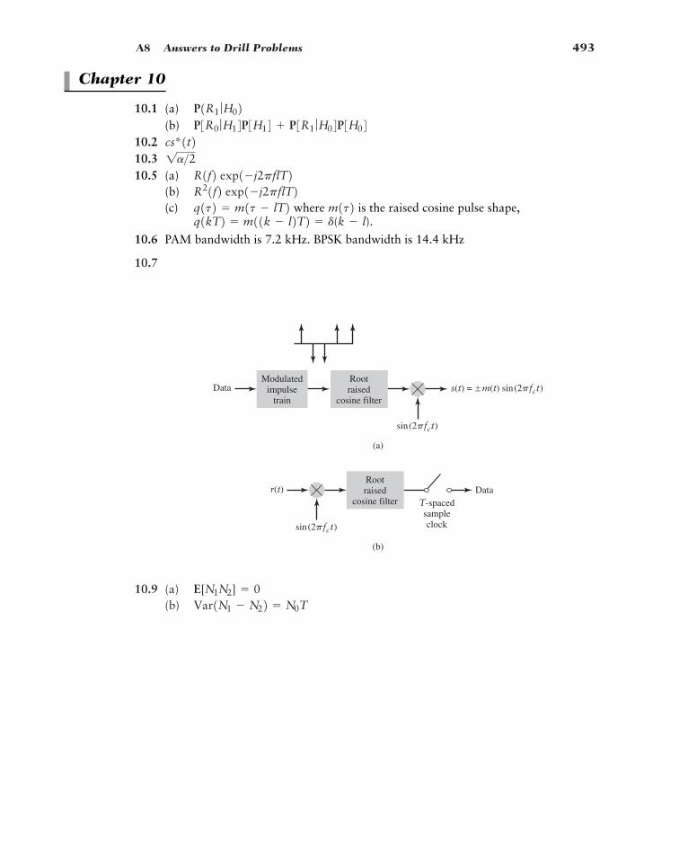
A8 Answers to Drill Problems 493
s(t) = —m(t) sin(2�fct)Modulated
impulsetrain
Rootraised
cosine filterData
sin(2�fct)
(a)
(b)
Rootraised
cosine filter T-spacedsampleclock
Datar(t)
sin(2�fc t)
Chapter 10
10.1 (a)(b)
10.210.310.5 (a)
(b)(c) where is the raised cosine pulse shape,
10.6 PAM bandwidth is 7.2 kHz. BPSK bandwidth is 14.4 kHz
q1kT2 � m11k � l2T2 � d(k � l).m1t2q1t2 � m1t � lT2R21f2 exp1�j2pflT2R1f2 exp1�j2pflT21a>2cs*1t2P3R0 ƒH14P3H14 P3R1 ƒH04P3H04
P1R1 ƒH02
10.7
10.9 (a)(b) Var1N1 � N22 � N0T
E[N1N2] � 0
Chapter 11
11.1 watts and 6.3 millivolts11.2 watts11.3 2610ºK11.4 and11.5 9.97 dB11.6 53.0 dB and 43.5 dB11.711.8 120ºK, 14.7 dB, and 13 dB11.9 13.9 m
11.10 132 dB and 101 dB11.11 Rmedian � 0.83Rrms
�143 dBW
�122 dBm>Hz�147 dBm>Hz
8 10�154 10�12
494 APPENDIX 8 � ANSWERS TO DRILL PROBLEMS
GLOSSARY
Functions
1. Rectangular functions
2. Unit step function
3. Signum function
4. (Dirac) delta function
or, equivalently,
5. Sinc function
6. Sine integral
7. Q-function
8. Binomial coefficient
9. Bessel function of the first
kind of order n
AbbreviationsA ampereac alternating currentADC analog-to-digital converterAM amplitude modulationASK amplitude-shift keyingb/s bits/secondBER bit error rateBFSK binary frequency-shift keyingBPF band-pass filterBPSK binary phase-shift keying
Jn1x2 �1
2p Lp
�p exp1jx sin u � jnu2 du
ankb �
n!1n � k2!k!
Q1x2 �1
22p Lq
x exp¢�
u2
2≤ du
Si1x2 � Lx
0
sin uu
du
sinc1x2 �sin1px2px
Lq
�qg1t2d1t � t02 dt � g1t02
Lq
�qd1t2 dt � 1
d1t2 � 0, t 0
sgn1t2 � c 1, t � 00, t � 0
�1, t � 0
u1t2 � b1, t � 00, t � 0
rect1t2 � b1, � 12 � t � 1
2
0, ƒt ƒ � 12
495
BSC binary symmetric channelcodec coder/decoderCW continuous waveDAC digital-to-analog converterdB decibeldBW decibel referenced to 1 wattdBmW decibel reference to 1 milliwattdc direct currentDFT discrete Fourier transformDM delta modulationDPCM differential pulse-code modulationDPSK differential phase-shift keyingDSB-SC double sideband-suppressed carrierexp exponentialFDM frequency-division multiplexingFFT fast Fourier transformFSK frequency-shift keyingFM frequency modulationGMSK Gaussian filtered MSKGSM global system for mobile communicationsHDTV high-definition televisionHz hertzIDFT inverse discrete Fourier transformIF intermediate frequencyIP internet protocolISI intersymbol interferenceISO International Organization for StandardizationLDM linear delta modulationlog logarithmLPF low-pass filtermodem modulator–demodulatorms millisecond
microsecondMSK minimum shift keyingNRZ nonreturn-to-zeroNTSC National Television Systems CommitteeOFDM orthogonal frequency-division multiplexingOOK on–off keyingOQPSK offset quadriphase-shift keyingOSI open systems interconnectionPAM pulse-amplitude modulationPCM pulse-code modulationPDM pulse-duration modulation
ms
496 GLOSSARY
PLL phase-locked loopPM phase modulationPPM pulse-position modulationPSK phase-shift keyingPWM pulse-width modulationQAM quadrature amplitude modulationQPSK quadriphase-shift keyingRF radio frequencyRZ return-to-zeros secondSNR signal-to-noise ratioTDM time-division multiplexingTV televisionUWB ultra widebandV voltVLSI very-large-scale integrationW watt
Glossary 497
BIBLIOGRAPHY
Abbate, J., Inventing the Internet, Cambridge, MA: The MIT Press, 1999.Anderson, J. B., Digital Transmission Engineering, IEEE Press, 1999.Abramowitz, M., and I. A. Stegun, Handbook of Mathematical Functions with Formulas,Graphs, and Mathematical Tables, New York: Dover, 1965.Arazi, B., A Commonsense Approach to the Theory of Error Correcting Codes, Cam-bridge, MA; The MIT Press, 1988.Bahai, A. R. S., and B. R. Saltzberg, Multi-carrier Digital Communications: Theory andApplications of OFDM, Kluwer, 1999.Baran, P., “Packet switching,” in J. C. McDonald, editor, Fundamentals of Digital Switch-ing, 2nd ed., pp. 193–235, New York: Plenum, 1990.Bell, D. A., Noise and Solid State, Plymouth, Eng.: Pentech Press, 1985.Bennett, W. R., Introduction to Signal Transmission, New York: McGraw-Hill, 1970.Bertsekas, D. M., and J. N. Tsitsiklis, Introduction to Probability, Athena Scientific, 2002.Blackman, N. M., Noise and Its Effect on Communication, New York: McGraw-Hill,1966.Black, H. S., Modulation Theory, Princeton, NJ: Van Nostrand, 1953.Blahut, R. E., Theory and Practice of Error Control Codes, Reading, MA: Addison-Wesley,1983.Bracewell, R. N., The Fourier Transform and Its Applications, 2nd ed., New York:McGraw-Hill, 1986.Carlson, A. B., Communications Systems, 2nd ed., New York: McGraw-Hill, 1975.Cassioli, D., M. Z. Win, and A. F. Molisch, “The ultra-wide bandwidth indoor channel:from statistical model to simulations,” IEEE Journal Selected Areas in Communications,vol. 20, pp. 1247–1257, 2002.Chung, K. L., Elementary Probability Theory with Stochastic Processes, New York:Springer-Verlag, 1979.Clark, G. C. Jr., and J. B.Cain, Error Correction Coding for Digital Communications, NewYork: Plenum, 1981.Cooley, J. W., “How the FFT gained acceptance,” IEEE Signal Processing Magazine, vol.9, no. 1, pp. 10–13, January 1992.Catternole, K. W., Principles of Pulse-code Modulation (New York: American Elsevier,1969).Cover, T., and J. Thomas, Elements of Information Theory, New York: Wiley, 1991.Downing, J. J., Modulation Systems and Noise, Englewood Cliffs, NJ: Prentice Hall, 1964.Erickson, G., “A fundamental introduction to the compact disc player,”http://www.tc.umn.edu/~erick205/Papers/paper.html#strengths.Gitlin, R. A., J. F. Hayes, and S. B. Weinstein, Data Communication Principles, New York:Plennum, 1992.Gold, B. and N. Morgan, Speech and Audio Signal Processing, New York: Wiley, 1999.Guttman, I., S. S. Wilks, and J. S. Hunter, Introductory Engineering Statistics, 2nd ed.,New York: Wiley, 1971.Haykin, S., Adaptive Filter Theory, 4th ed., Upper Saddle River, NJ: Prentice-Hall, 2002.Haykin, S., Communications Systems, 4th ed., New York: Wiley, 2001.Haykin, S., Communication Systems, 3rd ed., New York: Wiley, 1994.
498
Haykin, S., and M. Moher, Modern Wireless Communications, New Jersey: Prentice Hall,2005.James, J. H., B. Chen, and L. Garrison, “Implementing VoIP: a voice transmission perfor-mance progress report,” IEEE Communications Magazine, vol. 42, no. 7, pp. 36–41, July2004.Jayant, N. S., and P. Noll, Digital Coding of Waveforms: Principles and Applications inSpeech and Video, Englewood Cliffs, NJ: Prentice-Hall, 1984.Jeruchim, M. C., P. Balaban, and K. S. Shanmugan, Simulation of Communication Sys-tems, 2nd ed., New York: Plenum, 2000.Kammler, D. W., A First Course in Fourier Analysis, Upper Saddle River, NJ: Prentice-Hall,2000.Kaneko, H. “A unified formulation of segment companding laws and synthesis of codes anddigital componders”, Bell System Tech. J., vol. 49, pp. 1555–1588, 1970.Karlin, S. and H. M. Taylor, A First Course in Stochastic Processes, 2nd ed., New York:Academic Press, 1975.Lathi, B. P., Modern Digital and Analog Communication Systems, 3rd ed., Oxford: OxfordUniversity Press, 1998.Leon-Garcia, A., Probability and Random Processes for Electrical Engineering, 2nd ed.,Reading, MA: Addison-Wesley, 1994.Lin, S., and D. J. Costello, Error Control Coding, 2nd ed., Upper Saddle River, NJ: Prentice-Hall, 2004.Lucky, R. W., J. Salz, and E. J. Weldon, Principles of Data Communication, New York:McGraw-Hill, 1968.Madisetti, V. K., and D. B. Williams, editors, The Digital Signal Processing Handbook,CRC Press, 1998.McDonald, J. C. ed. Fundamentals of Digital Switching, 2nd edition New York: Plennum,1990.McEliece, R. J., The Theory of Information and Coding, Reading, MA: Addison-Wesley,1977.Middleton, D., An Introduction to Statistical Communication Theory, New York: McGraw-Hill, 1960.Papoulis, A., Probability, Random Variables, and Stochastic Processes, 2nd ed., New York:McGraw-Hill, 1984.Pratt, T., and C. W.Bostian, Satellite Communications, New York: Wiley, 1986.Proakis, J. G., Digital Communications, 3rd ed., New York: McGraw-Hill, 1999.Robinson, F. N., Noise and Fluctuations in Electronic Devices and Circuits, Oxford: Claren-don Press, 1974.Shannon, C. E., “A mathematical theory of communication,” Bell System Technical Jour-nal, vol. 27, pp. 379–423, 623–256, July, October, 1948.Smith, B. “Instantaneous companding of quantized signals”, Bell System Tech. J., vol. 36,pp. 653–709, 1957.Special Issue, “The Internet: past, present, and future,” IEEE Communications Magazine,vol. 40, no. 7, pp. 42–76, July 2002.Steele, R. E., and L. Hanzo, Mobile Radio Communications, 2nd ed., New York: Wiley,1999.Sveshnikov, A. A. (ed.), Problems in Probability Theory, Mathematical Statistics and The-ory of Random Functions, New York: Dover Publications, 1968.Takahashi, A., and H. Yoshino, “Perceptual QoS assessment of technologies for VoIP,”IEEE Communications Magazine, vol. 42, no. 7, pp. 28–34, July 2004.
Bibliography 499
Tannenbaum, A. S., Computer Networks, 3rd ed., Englewood Cliffs, NJ: Prentice-Hall,1996.Thomas, J. B., An Introduction to Applied Probability and Random Processes, New York:Wiley, 1971.Van Der Ziel, A., Noise: Sources, Characterization, Measurement, Englewood Cliffs, NJ:Prentice Hall, 1970.Willner, A. E., “Mining the optical bandwidth for a terabit per second,” IEEE Spectrum,vol. 34, pp. 32–41, April 1997.Win, M. Z., and R. A. Scholtz, “Impulse radio: how it works,” IEEE Comm. Letters, vol.2, pp. 36–38, 1998.Wozencraft, J. M. and I. M. Jacobs, Principles of Communication Engineering, New York:Wiley, 1965. Reprinted by Waveland Press, Prospect Heights: Illinois, 1990.Wylie, C. R. and L. C. Barrett, Advanced Engineering Mathematics, 5th edition (NewYork: McGraw-Hill, 1982).Yuen, J. H. (ed.), Deep Space Telecommunications Systems Engineering, New York: Plenum,1983.Zeimer, R. E., and W. H. Tranter, Principles of Communications: Systems, Modulation andNoise, 5th ed., New York: Wiley, 2002.
500 BIBLIOGRAPHY
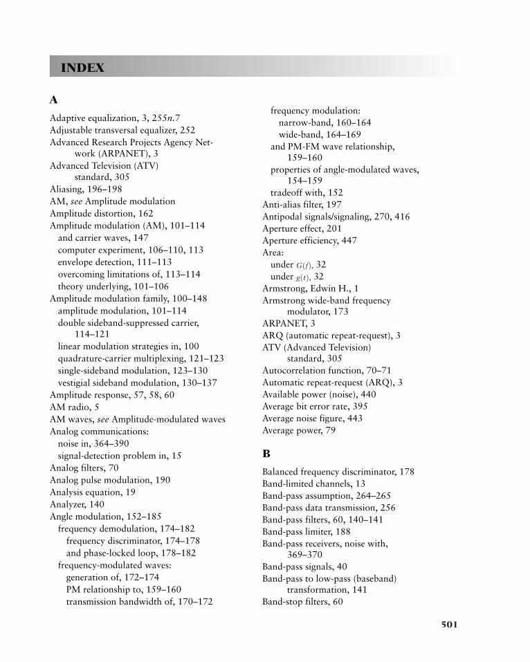
INDEX
A
Adaptive equalization, 3, 255n.7Adjustable transversal equalizer, 252Advanced Research Projects Agency Net-
work (ARPANET), 3Advanced Television (ATV)
standard, 305Aliasing, 196–198AM, see Amplitude modulationAmplitude distortion, 162Amplitude modulation (AM), 101–114
and carrier waves, 147computer experiment, 106–110, 113envelope detection, 111–113overcoming limitations of, 113–114theory underlying, 101–106
Amplitude modulation family, 100–148amplitude modulation, 101–114double sideband-suppressed carrier,
114–121linear modulation strategies in, 100quadrature-carrier multiplexing, 121–123single-sideband modulation, 123–130vestigial sideband modulation, 130–137
Amplitude response, 57, 58, 60AM radio, 5AM waves, see Amplitude-modulated wavesAnalog communications:
noise in, 364–390signal-detection problem in, 15
Analog filters, 70Analog pulse modulation, 190Analysis equation, 19Analyzer, 140Angle modulation, 152–185
frequency demodulation, 174–182frequency discriminator, 174–178and phase-locked loop, 178–182
frequency-modulated waves:generation of, 172–174PM relationship to, 159–160transmission bandwidth of, 170–172
frequency modulation:narrow-band, 160–164wide-band, 164–169
and PM-FM wave relationship, 159–160
properties of angle-modulated waves,154–159
tradeoff with, 152Anti-alias filter, 197Antipodal signals/signaling, 270, 416Aperture effect, 201Aperture efficiency, 447Area:
under 32under 32
Armstrong, Edwin H., 1Armstrong wide-band frequency
modulator, 173ARPANET, 3ARQ (automatic repeat-request), 3ATV (Advanced Television)
standard, 305Autocorrelation function, 70–71Automatic repeat-request (ARQ), 3Available power (noise), 440Average bit error rate, 395Average noise figure, 443Average power, 79
B
Balanced frequency discriminator, 178Band-limited channels, 13Band-pass assumption, 264–265Band-pass data transmission, 256Band-pass filters, 60, 140–141Band-pass limiter, 188Band-pass receivers, noise with,
369–370Band-pass signals, 40Band-pass to low-pass (baseband)
transformation, 141Band-stop filters, 60
g1t2,G1f2,
501
Bandwidth, 39–40and amplitude response, 58channel, 13definitions of, 40and inverse relationship between time
and frequency, 40–41and time-bandwidth product, 41
Bandwidth-conservation system, 121Bandwidth-duration product, 41Baran, P., 7n.2Bardeen, John, 2Baseband, 137Baseband data transmission, 231–256
computer experiment, 249–251eye pattern in, 246–251intersymbol interference problem in,
233–234of M-ary data, 245and Nyquist channel, 235–237and raised-cosine pulse spectrum,
238–245roll-off portion of spectrum, 241–243root raised-cosine pulse spectrum,
244–245transmission-bandwidth requirement,
240–241Baseband representation:
of band-pass filters, 140–141of modulated waves, 137–140
Base resistance, thermal noise from, 442Base station (satellite
communications), 6Basic group (multiplexing), 146–147BASK, see Binary amplitude-shift keyingBBC (British Broadcasting Corporation), 2Beat (signal), 149Bel, 459Bell, Alexander Graham, 2, 459n.1Bell Laboratories, 2, 4BER, see Bit error rateBerners-Lee, Tim, 3Bernoulli distribution function, 319Bernoulli random variable, 318, 328Bessel functions, 165, 467–469Best effort service (Internet), 10, 11BFSK, see Binary frequency-shift keying
BIBO, see Bounded input-bounded outputstability criterion
Binary amplitude-shift keying (BASK), 263,265–269
generation/detection of signals, 265–266spectral analysis of, 266–269, 399–404
Binary frequency-shift keying (BFSK), 263,281–282
detection of, 414–415Binary phase-shift keying (BPSK), 263,
270–274generation/coherent detection
of signals, 270–271optimum detection of, 405–408spectral analysis of, 271–274
Binomial distribution, 321Bipolar chopper, 228Bipolar return-to-zero (BRZ)
signaling, 219Bit duration, 263Bit error rate (BER), 395–396, 419–420Bit reversal, 88Block codes, 424–426, 430–431Boresight, 447Bose—Chaudhuri—Horcquenghem block
codes, 430Bounded input-bounded output (BIBO)
stability criterion, 55–56BPSK, see Binary phase-shift keyingBranches (signal-flow graph), 85–87Brattain, Walter H., 2British Broadcasting Corporation (BBC), 2Broadcasting, 4BRZ (bipolar return-to-zero)
signaling, 219Burst noise, 438Butterworth filters, 70, 249
C
Carrier-frequency tuning, 142Carrier power (satellite systems), 449Carrier-to-noise ratio (CNR), 450–451Carrier wave, 14Carson’s rule, 170Cartesian representation, 162Causal systems, 55
502 INDEX
CDs (compact discs), 12Central limit theorem, 333–335Channels:
band-limited, 13defined, 53power-limited, 13
Channel bandwidth, 13, 14Channel bits, 423, 429Channel noise, 13Chebyshev filters, 70Circuit switching, 7Clark, Arthur C., 4Closed-loop feedback system, 178Closed-loop gain, 180n.3CNR, see Carrier-to-noise ratioCode rate, 431Coherent detection, 116, 134
binary phase-shift keying, 270–271double sideband-suppressed carrier
modulation, 116–118of the DSB-SC modulated wave, 184noise in linear receivers using,
370–373with single-sideband modulation,
127–128with vestigial sideband modulation,
134–135Communication network, 6–8Communication systems:
basic types of, 4–5communication networks, 6–8composition of, 5data networks, 8–9data storage, 12design parameters for, 14historical background of, 1–4integration of telephone and Internet,
11–12Internet, 9–11noise in, 365–366operational requirements for, 13–14performance improvement for, 14primary resources in, 13radio, 5–6theories underlying, 14–16
Compact discs (CDs), 12
Complementary error function, Q-functionand, 471–472
Complex carrier wave, 138Complex envelope:
of the FM waves, 165of the modulated wave, 138
Complex exponential Fourier series, 50,461–462
Complex exponential function, applicationof delta function to, 45–46
Complex Fourier coefficient, 50Complex low-pass filter, 141Computer networks, 3–4, 6–8Comte, Auguste, 1Conditional probability, 323–326Conjugation rule (Fourier transforms),
28–29Connection delay (Internet), 11Constants, 479Continuous amplitude spectrum, 21Continuous Fourier transform, see Fourier
transform (FT)Continuous-phase frequency-shift keying
(CPFSK), 282–283Continuous-phase signal, 281Continuous phase spectrum, 21Continuous spectrum, 51Continuous-wave (CW) modulation, 100
amplitude modulation, 100–148angle modulation, 152–185families of, 100pulse modulation vs., 190
Convolutional codes, 430–431Convolution integral, 37, 54Convolution theorem (Fourier transforms),
37Correlation, 38Correlation receiver, 399Correlation theorem (Fourier transforms),
37–38Correlative coding, 259Costas receiver, 120–121Covariance, 328–329CPFSK, see Continuous-phase frequency-
shift keyingCross-correlation function, 77–78Cross-spectral density, 78
Index 503
CW modulation, see Continuous-wavemodulation
D
Datagrams, 10Data networks, 8–9Data storage, 12dBs, see Decibelsdc signal, application of delta function
to, 45Decibels (dBs), 13, 459Decimation-in-frequency algorithm, 88Decimation-in-time algorithm, 88Decision thresholds/levels, 205Decoder, 424De-emphasis filter, 388–389Deep-space links, 13De Forest, Lee, 2Delta function, see Dirac delta functionDelta modulation (DM), 211–216
delta-sigma modulation, 215–216quantization errors, 214–215
Demultiplexed components, 276Demultiplexing system, 184Detection theory, 15Deviation ratio, 171DFT, see Discrete Fourier transformDibit, 274Difference-frequency term, 179Differential encoding, 219Differential pulse-code modulation
(DPCM), 216–219Differentiation in the time domain
(Fourier transforms), 32–34Diffraction, in terrestrial mobile
radio, 451, 452Digital Advanced Television (ATV)
standard, 305Digital band-pass modulation techniques,
262–309band-pass assumption
in, 264–265binary amplitude-shift keying, 265–269frequency-shift keying, 281–289mapping of waveforms onto constella-
tions of signal points, 299–301
M-ary digital modulation schemes,295–299
noncoherent detection schemes, 291–295BASK signals, 291–292BFSK signals, 292–293differential phase-shift keying, 293–294
phase-shift keying, 270–281Digital communication:
history of, 2–3noise in, 394–434signal-detection problem in, 15
Digital filters, 70Digital pulse modulation, 190, 204Digital radio, 5Digital subscriber line (DSL), 11, 302Digital switching, 7Digital television, 6, 305–307Digital versatile discs (DVDs), 12Dilation property (Fourier
transforms), 28Diode equation, 441Dirac comb, 51–52Dirac delta function, 42–50
applications of, 45–50and extension of Fourier
transform, 42in the frequency domain, 103as limiting form of Gaussian pulse, 43–45replication property of, 43sifting property of, 42
Direct method (FM wave generation),172–173
Dirichlet conditions, 20, 42Discrete Fourier transform (DFT),
18, 81and FFT, 83–84interpretation of, 82–83
Discrete memoryless channel, 324Discrete spectrum, 51, 462–464Discrete-time filter, 217Discrete-time Fourier transform, 194–196Discrete-time signal processing, 204Distribution functions, 318–320DM, see Delta modulationDouble exponential pulse, 26–27Double-frequency term, 179
504 INDEX
Double sideband-suppressed carrier (DSB-SC) modulation, 113–121
coherent detection, 116–118, 370–373computer experiment, 118–120Costas receiver for detection of, 120–121theory underlying, 114–116
Doublet pulse, 34Downlink (communications), 6DPCM, see Differential pulse-code
modulationDSB-SC modulation, see Double sideband-
suppressed carrier modulationDSL, see Digital subscriber lineDuty cycle, 463DVDs (digital versatile discs), 12
E
Earth-orbiting satellite, 4Eckert, J. Presper, Jr., 3Effective aperture area, 447Effective isotropic radiated power (EIRP),
448Electrical noise:
available noise power, 440shot noise, 440–442thermal, 438–440
Electromagnetic theory of light, 1Electronics, history of, 2Elementary event, 315E-mail messages, 11Encoder, 424Energy gap (in SSB modulation), 114Energy signals, 70–78
autocorrelation function of, 70–71cross-correlation of, 77–78defined, 20energy spectral density of, 71–77Fourier transformability of, 20Wiener—Khitchine relations
for, 71–72Energy spectral density, 71–77
defined, 71effect of filtering on, 72–75of energy signals, 71–77interpretation of, 75–77and use of filters, 72–75
ENIAC, 3Ensembles, signal, 16Envelope detectors/detection, 103
amplitude modulation, 111–113for AM wave demodulation, 111noise in AM receivers using, 373–377for sinusoidal AM, 113of VSB plus carrier, 136
Envelope distortion, 102–103Equalization, 251–255
adaptive, 3, 255n.7in pulse-amplitude modulation,
200–202zero-forcing, 253–255
Equivalent noise temperature, 443–445
Error correction capability, 425Error detection and correction
(digital systems noise), 422–433block codes, 424–426, 430–431Bose—Chaudhuri—Horcquenghem
block codes, 430convolutional codes, 430–431Hamming codes, 426–430Reed—Solomon block codes, 430signal-space interpretation of codes,
431–433turbo codes, 431
Error propagation phenomenon, 260Error syndrome, 428Euler’s formula, 31, 46Excess bandwidth, 241Excitation, 52Expectation, statistical averages of,
326–329Exponential pulse(s), 23–25
double, 26–27truncated decaying, 23–24truncated rising, 24–25
External noise, 437Eye patterns, 246–251
for M-ary transmission, 249peak distortion for intersymbol
interference, 247–249timing features for, 247
Index 505
F
Farnsworth, Philo T., 2Fast Fourier transform (FFT), 15, 83–88FDM, see Frequency-division multiplexingFeed-back, 173Fessenden, Reginald, 1FFT, see Fast Fourier transformFigure of merit, 373, 376, 379, 385Filters, 60
analog, 70Butterworth, 70Chebyshev, 70defined, 53, 60digital, 70and energy spectral density, 72–75ideal low-pass filters, 60–70for superheterodyne receivers, 142noise equivalent bandwith, 354–356
First detector, 143First order phase-locked loop, 182Fleming, John Ambrose, 2Flicker noise, 438FM, see Frequency modulationFM radio, 1, 5FM waves, see Frequency-modulated
wavesForward-error-correction codes,
431–433Fourier, Joseph, 19n.1Fourier analysis, 15Fourier series, 19n.1, 460–464
complex exponential, 50, 461–462and discrete spectrum, 462–464
Fourier transform(s), 18–52, 464–466. See also specific headings, e.g.:Fast Fourier transform
and area under 32and area under 32and conjugation rule, 28–29and convolution theorem, 37and correlation theorem, 37–38defined, 15, 19and differentiation in the time domain,
32–34dilation property of, 28and Dirac delta function, 42–50
g1t2,G1f2,
duality of, 29–30frequency-shifting property of, 30–32and integration in the time domain,
34–36inverse, 19and inverse relationship between time
and frequency, 39–41linearity of, 25–28and modulation theorem, 36–37notations in, 20–21numerical computation of, 81–89
DFT and IDFT, interpretation of, 82–83
FFT algorithms, 83–88IDFT, computation of, 88–89
of periodic signals, 50–52properties of, 475and pulse signal as continuous sum
of exponential functions, 21–25
and Rayleigh’s energy theorem, 38–39theorems, 475time-shifting property of, 30
Fourier-transform pairs, 19, 21, 476Free-space link calculations, 446–451
carrier-to-noise ratio, 450–451received signal power, 447–450
Free-space loss, 448Free-space propagation, 451Frequency:
fundamental, 50inverse relationship between time
and, 39–41Frequency content (of a signal), 18Frequency demodulation, 174–182
frequency discriminator, 174–178and phase-locked loop, 178–182
Frequency deviation, 161Frequency discrimination method,
125–127Frequency discriminator, 175Frequency-division multiplexing (FDM),
145–146modulation steps for, 146–147orthogonal, 302–304stereo multiplexing, 182–184
506 INDEX
Frequency-modulated radar, 185Frequency-modulated (FM) waves,
154–159generation of, 172–174PM relationship to, 159–160transmission bandwidth of, 170–172
Frequency modulation (FM), 154detection of, 380–387narrow-band, 160–164origin of concept, 1wide-band, 164–169
Frequency multiplier, 173Frequency resolution, 81Frequency response (in linear systems),
56–58Frequency-sensitivity factor, 154Frequency-shifting property
(Fourier transforms), 30–32Frequency-shift keying, 281–289
binary, 281–282continuous-phase, 282–283detection of, 414–416minimun-shift keying, 283–289
Friis transmission formula, 448, 454Fundamental frequency, 50
G
Gauss, C. G., 330n.4Gaussian monocycle, 223Gaussian processes, 347–348Gaussian pulse:
defined, 33delta function as limiting form
of, 43–44as unit pulse, 34
Gaussian random variables, 330–333Generalized functions (generalized
distributions), 43Generating functions, 50Geostationary orbit, 6, 446Ghosting, 452Global System for Mobile (GSM)
Communications, 304Gray encoding, 418GSM (Global System for Mobile
Communications), 304
H
Hamming, R., 422n.3Hamming codes, 426–430Hamming distance, 424–425Hamming weight, 424Hand-held devices (for Internet
access), 11Harmonic distortion, 162HDTV, 6Heat flow, 19n.1Hertz, Heinrich, 1High-definition television (HDTV), 6High-pass filters, 60Hilbert transform, 98–99, 139n.4(i)Hilbert-transform pairs, 476Hockham, G. A., 4Hold-in frequency range, 182Hosts, 7, 10HTML, 3HTTP, 3Hybrid modulated wave, 177Hypertext markup language (HTML), 3Hypertext transfer protocol (HTTP), 3Hypothesis testing, 15
I
IC (integrated circuit), 2I-channel, 120–121Ideal low-pass filters, 60–70
approximation of, 69–70pulse response of, 61–69
Ideal sampling function (Dirac comb),51–52
IDFT, see Inverse discrete Fourier transform
Image interference (in superhet receivers), 143
Image signals:suppressing, 143as two-dimensional function
of time, 5Impossible event, 315Impulse radio, 223–224Impulse response, 53Independent Bernoulli trials, 321
Index 507
Indirect method (FM wave generation), 173Information-bearing (message) signal, 101Information bits, 423Initial-echo control (in VoIP), 12Inphase coherent detector (I-channel),
120–121In-phase path (SSB modulators), 127In-place computation, 88Instantaneous sampling, 191–193Integrals, 478Integrate-and-dump detector, 400Integrated circuit (IC), 2Integration in the time domain (Fourier
transforms), 34–36, 49–50Interfaces (OSI model), 8Internal noise, 437Internet, 9–12Internet protocol (IP), 10Interpolation formula, 195, 235Intersymbol interference problem,
233–234Inverse discrete Fourier transform
(IDFT), 82computation of, 88–89interpretation of, 82–83
Inverse Fourier transform, 19Inverse Hilbert transform, 98IP (Internet protocol), 10
J
Joint probability density function, 320
K
Kao, K. C., 4k-by-n generator matrix, 427
L
Laser, 4Layered architecture, 8Linear delta modulators, 214Linearity of Fourier transforms, 25–28Linear receivers, noise in, 370–373Linear system, 52Linear time-invariant (LTI) systems,
18, 54–55
Line codes (pulse modulation), 219–220Line-of-sight radio propagation, 6Link budget, 449–450List decoder, 427Lodge, Oliver, 1Logic network, 293Loop filter, 178Loop-gain parameter, 180Lower sideband, for positive
frequencies, 103Low-pass filters, 60. See also Ideal
low-pass filtersLow-pass signals, 40–41, 98Low-pass transfer function, 131–133LTI systems, see Linear time-invariant sys-
temsLucky, Robert, 3
M
Main lobe, 40Manchester code, 219Mapping process, 6Marconi, Guglielmo, 1Marginal densities, 320M-ary amplitude shift keying
(M-ary ASK), 297M-ary data transmission, 249
baseband, 245eye patterns for, 249, 411–412
M-ary digital modulation schemes:frequency-shift keying, 298–299phase-shift keying, 295–297quadrature amplitude modulation,
297–298, 411–414Mastergroups (multiplexing), 147Matched filter, 3, 396–397Mathematical constants, 479Mathematical tables, 475–479MATLAB scripts (computer experiments),
480–487Mauchly, John W., 3Maximum-power transfer theorem, 440Maxwell, James Clerk, 1Mean-square error criterion, 255n.7Mean-square value, 345Median path loss, 453–454
508 INDEX
Message bandwidth, 103, 130Message signal, 101Message spectrum, 103Microprocessors, 2Middleton, D., 3Minimum-shift keying (MSK),
283–289formulation of, 286–287power spectrum evaluation, 287–289
Mobile radio, terrestrial, 451–452Modulated waves, baseband representation
of, 137–140Modulation. See also specific types, e.g.:
Pulse modulationdefined, 14, 100primary motivation for, 100
Modulation factor, 104Modulation index, 161Modulation theorem (Fourier transforms),
30, 36–37Modulation theory, 14Modulo-two addition, 260Morse, Samuel, 1Morse Code, 1MSK, see Minimum-shift keyingMulti-carrier system, 302Multipath phenomenon (wireless
communications), 6, 451–456Multiplexing, 145Multiplier (phase-locked loops), 178
N
Narrowband, 111Narrow-band frequency modulation,
160–164Narrowband noise, 352–356Natural sampling, 228Near-phase-lock, 179Negative feedback amplifier, 180n.3Nodes (signal-flow graph), 85–87Noise, 437–457
in analog communication, 364–390in AM receivers using envelope
detection, 373–377with band-pass receiver structures,
369–370
detection of frequency modulation,380–387
FM pre-emphasis/de-emphasis,387–390
in linear receivers using coherentdetection, 370–373
signal-to-noise ratios, 366–369in SSB receivers, 377–379
cascade connection of two-port networks,445–446
in communications systems, 365–366defined, 13, 313, 364in digital communication, 394–434
bit error rate, 395–396detection of QAM, 411–414detection of QPSK, 408–411detection of single pulse, 396–399differential detection, 416–418error detection and correction, 422–433Gray encoding, 418optimum detection of binary PAM,
399–405optimum detection of BPSK, 405–408optimum detection of FSK, 414–416performance comparison of strategies,
419–420in signal-space models, 421–422
electrical, 438–442equivalent noise temperature, 443–445external vs. internal, 437free-space link calculations, 446–451narrowband, 352–356noise figure, 442–443sources of, 437with terrestrial mobile radio, 451–456white, 348–351
Noise-equivalent bandwidth, 354–356Noise figure, 442–443Noise spectral density, 444–445Noncoherent detection, 291–295
BASK signals, 291–292BFSK signals, 292–293differential phase-shift keying, 293–294,
416–418Non-return-to-zero level encoder, 270,
275–276
Index 509
Nonreturn-to-zero (NRZ) signaling, 219Nonuniform quantizer, 207Normalized root-raised cosine pulse
shape, 404Normal random variables, 330n.5North, D. O., 3Norton equivalent circuit, 439Noyce, Robert, 2NRZ (nonreturn-to-zero) signaling, 219nth order Bessel function, 165–166Nulls, 40Null event, 315Null-to-null bandwidth, 40Nyquist, Harry, 2, 243n.3Nyquist channel, 235–237
O
Odd-symmetric time function, 27Okumura—Hata model, 453n.8One-bit delay element, 293“One-over-f” noise, 438On-off signaling, 219Open-loop gain, 180n.3Open system interconnection (OSI)
reference model, 8, 9Optical communications, history of, 4Optimum pulse shape, 235Orthogonal frequency-division multiplex-
ing, 302–304Orthogonal signaling, 416OSI model, see Open system interconnec-
tion reference model
P
Packets, 8, 10Packet loss ratio, 11Packet-switched networks, 8Packet switching, 3, 7–8Paley-Wiener criterion, 58PAM, see Pulse-amplitude modulationPartial-response signaling, 259Passband, 60Path loss, 448, 453–454PBXs (private branch exchanges), 12PCM, see Pulse-code modulation
PCs (personal computers), 3PDM, see Pulse-duration modulationPeer processes, 8, 9Percentage modulation, 103, 104Periodicity, 51, 84Periodic signals, 124
Fourier transforms of, 50–52in linear systems, 52–59
Periodogram, 80Personal computer (PCs), 3Phase discrimination method (SSB
generation), 127Phase discriminator (I- and
Q-channels), 121Phase error, 179Phase-lock, 179Phase-locked loop, 178–182Phase-modulated (PM) waves, 154–159Phase modulation (PM), 153Phase noise, 362Phase response, 57, 60Phase sensitivity factor, 153Phase-shift keying, 270–281
binary, 270–274quadriphase, 274–281
Physical constants, 479Physical layer, 9Pierce, John R., 4Pilot, for VSB modulated wave
detection, 136n.3Pilot-assisted training, 255, 307Pixels, 5PM (phase modulation), 153PM waves, see Phase-modulated wavesPoint-to-point communications, 4–5, 147Poisson’s sum formula, 51Polar representation, 162Post-detection signal-to-noise ratio, 368
in AM receivers using envelope detection,374–376
in FM modulation, 381–385in linear receivers, 372–373in SSB receivers, 378–379
Power, transmitted, 13Power budget, 449Power-limited channels, 13
510 INDEX
Power ratios, 459Power spectral density, 79–81, 344–346PPM (pulse-position modulation), 203Pre-detection signal-to-noise ratio, 368
in AM receivers using envelope detection, 374
in FM modulation, 380–381in linear receivers, 371in SSB receivers, 378
Prediction, 217Private branch exchanges (PBXs), 12Probability theory, 16, 314–335
axioms of probability, 315–316central limit theorem, 333–335conditional probability, 323–326distribution functions, 318–320Gaussian random variables, 330–333random variables, 317–318relative-frequency approach, 314–315several random variables, 320–323and statistical averages of expectation,
326–329and transformation of random
variables, 329–330Product modulator, 114Protocol (data networks), 8Pulse-amplitude modulation (PAM),
198–202aperture effect and equalization,
200–202binary, optimum detection
of, 399–405performance of, 419–420sample-and-hold filter, 199–200
Pulse-code modulation (PCM), 206–211
invention of, 2receiver operations, 211regeneration along transmission
path, 209–210transmitter operations, 206–209
Pulse-duration modulation (PDM),202–203
Pulse modulation, 190–226analog, 190continuous-wave modulation vs., 190delta modulation, 211–216
differential pulse-code modulation,216–219
digital, 190families of, 190line codes in, 219–220pulse-amplitude modulation, 198–202pulse-code modulation, 206–211pulse-duration modulation, 202–203pulse-position modulation, 203quantization process in, 205–206sampling process for:
and aliasing phenomenon, 196–198instantaneous sampling, 191–193sampling theorem, 193–196
Pulse-position modulation (PPM), 203Pulse response (ideal low-pass filters), 61–69
Q
QAM, see quadrature-amplitudemodulation
Q-factor, 178n.2Q-function, 331, 402, 470–472QoS (quality of service), 11QPSK, see Quadriphase-shift keyingQuadrature-amplitude modulation (QAM),
121–123, 414detection of, in noise, 411–414performance of, 419–420
Quadrature-carrier multiplexing, 121–123Quadrature null effect, 117Quadrature path (SSB modulators), 127Quadrature-phase coherent detector
(Q-channel), 121Quadriphase-shift keying (QPSK), 274–281
detection of, in noise, 408–411generation/detection of signals, 275–277offset, 277–281performance of, 419–420power spectra of signals, 278–281
Quality factor (Q-factor), 178n.2Quality of service (QoS), 11Quantization process:
in delta modulation, 214–215in pulse modulation, 205–206
Quantizer characteristics, 205Quantum, 205
Index 511
R
Radio, 5–6digital, 5history of, 1impulse, 223–224terrestrial mobile radio, 451–452
Radio frequency (RF) pulse, 31–32Radio receivers, superheterodyne, 1Raised-cosine pulse spectrum, 238–245
properties of, 241–244roll-off portion of spectrum, 241–243root raised-cosine pulse spectrum,
244–245transmission-bandwidth requirement,
240–241Random experiment, 314Random processes, 16, 335–343, 365
correlation of, 338–343stationary, 337–338
Random signals, 313–348defined, 16, 313and Gaussian processes, 347–348and probability theory, 314–335and random processes, 335–343
correlation of, 338–343stationary, 337–338
spectra of, 343–346Random variables, 317–318, 329–330
experiments with several, 320–323Gaussian, 330–333transformation of, 329–330
Rayleigh distribution function, 455Rayleigh fading, 454–456Rayleigh’s energy theorem, 38–39Real-time spectrum analyzer, 187Received signal power, 447–450Reconstruction levels, 205Rectangular pulse, 22–23Reed—Solomon block codes, 430Reeves, Alex, 2Reference power level, 459Reference signal-to-noise ratio, 368Reference transmission model, 368Reflection (terrestrial mobile radio),
451, 452Reflection property (Fourier transforms), 28
Representation levels, 205Response, defined, 52Return-to-zero (RZ) signaling, 219RF pulse, see Radio frequency pulserms bandwidth, see Root mean-square
bandwidthRms duration, 98Roll-off factor, 238, 256Root mean-square (rms) bandwidth,
40–41, 98Root mean-square (rms) duration, 98Root raised-cosine pulse spectrum,
244–245, 404–405Routers, 7, 10RZ signaling, 219
S
Sample point, 315Sampling theorem, 193–196, 235Satellite channels, 13Satellite communications:
components of, 6free-space link calculations
for, 446–451history of, 4as point-to-point system, 6system noise temperature
of receivers, 446Scanning, 5Scanning variable, 70Scatter diagram, 246n.4Schottky formula, 441Schwarz’s inequality, 473–474Search engines, 11Searching variable, 70Second detector, 143Series expansions, 477Shannon, Claude, 3, 422n.3Shockley, William, 2Shot noise, 438, 440–442Side-frequencies, 123Sifting property (of Dirac delta function),
42–43Signals. See also specific types, e.g.:
Periodic signalsand bandwidth, 40
512 INDEX
frequency content of, 18real-valued, conjugate symmetry
of spectra of, 22Signal-dependent phenomenon, 256Signal detection:
binary amplitude-shift keying, 265–266of binary PAM in noise, 399–405of BPSK, 405–408coherent:
binary phase-shift keying, 270–271double sideband-suppressed carrier
modulation, 116–118, 370–373linear receivers, 370–373
detection theory, 15differential, 416–418with frequency modulation, 380–387of FSK, 414–416noncoherent, 291–295
BASK signals, 291–292BFSK signals, 292–293differential phase-shift keying,
293–294of QAM, 411–414of QPSK, 408–411quadriphase-shift keying, 275–277signal-detection problem in, 15
Signal-detection problem, 15Signal-flow graph, 85–87Signal-space diagram, 296Signal-space interpretation of codes,
431–433Signal-space models, noise in,
421–422Signal-to-noise ratio (SNR), 13
in analog communication, 366–369post-detection, 368, 372–376, 378–379,
381–385as system design parameter, 14
Signum function, 27, 47–48Similarity property (Fourier
transforms), 28Sinc function, 22–23Sinc pulse, 29–30, 38–39Single-sideband (SSB) modulation,
113–114, 123–130and amplitude modulation, 147
coherent detection of, 127–128, 337–379frequency translation, 128–130modulators for, 125–127theory underlying, 123–125
Single-sideband receivers, noise in, 377–379Sinusoidal carrier waves, 14, 100. See also
Continuous-wave modulationSinusoidal DSB-SC spectrum, 116Sinusoidal functions, application of delta
function to, 46–47Sinusoidal modulating wave, SSB
modulation and, 123Sinusoidal VSB wave modulation, 133Slope circuit, 175Slope network, 380SNR, see Signal-to-noise ratioSpectral density:
cross-spectral density, 78energy, 71–77noise, 444–445power, 79–81
Spectral distortion, avoiding, 110Spectral overlap, 110Speech signals, digital encoding of, 2Speech vecoders, 395n.1Split-phase (Manchester code), 219Spot noise figure, 443Square law, 110Square-law modulator, 110, 111Square wave, 266SSB modulation, see Single-sideband
modulationStable systems, 55–56Stationary random processes, 337–338Step-by-step switch, 2Step-size, 205Stereo multiplexing, 182–184Stochastic processes, 16. See also
Random processesStopband, 60Stored-program system (telephone), 2Strowger, A. B., 2Strowger switch, 2Subnets, Internet, 10Summations, 478Sunde’s BFSK, 281–282
Index 513
Supergroup (multiplexing), 147Superheterodyne receivers (superhets), 1,
142–143, 369Superposition, principle of, 52Superposition of Fourier transforms,
25–28Sure event, 315Switching, 7
circuit, 7packet, 7–8
Symbol error rate, 413Synchonous demodulation, 116Synthesis equation, 19Synthesis filter, 195, 197Synthesizer, 140System, defined, 52Systematic convolutional code, 430–431System margin, 449System performance, 15
T
Tapped-delay-line filter, 54–55, 217TDM, see Time-division multiplexingTelegraph, 1Telephone channels, 13Telephone systems:
first commercial service, 2history of, 2integration of Internet and, 11–12twisted pairs, 89–90
Television:digital, 305–307high-definition, 6history of, 2transmissions for, 5
Television channels, 13Television signals, VSB modulation of,
143–145Terrestrial mobile radio, 451–452Thermal noise, 438–440Thévenin equivalent circuit, 4393-dB bandwidth, 40Threshold effect, 386–387Time, inverse relationship between
frequency and, 39–41Time-bandwidth product, 41, 69
Time-division multiplexing (TDM), 145,220–223
Time function:differentiation of a, 32–33integration of a, 34–36odd-symmetric, 27real and imaginary parts of a, 35–36
Time response, transmission of signalsthrough linear systems and, 53–55
Time-shifting property (Fourier transforms), 30
T-1 carrier system, 2, 222–223, 241Transistor, invention of, 2Transmission bandwidth (AM waves), 104Transmission lines, 89Transmission losses, 4Transmitted power, 13Transmitters, 5Transversal filter, 252Triangular pulse, 34–35Trigonometric identities, 477Truncated decaying exponential pulse,
23–24Truncated rising exponential
pulse, 24–25Turbo codes, 431Twiddle factor, 85Twisted pairs, 11, 89–90Two-port devices:
average noise figure of, 443equivalent noise temperature
of, 443–445Two-port networks, cascade connection
of, 445–446Type 1 error, 401
U
Ultra-wideband (UWB) radiotransmission, 223
Ungerboeck, G., 3Unit impulse, 42Unit prefixes, 479Unit pulse, 34Unit step function, 48–49Unity peak distortion, 248Uplink (communications), 6
514 INDEX
Upper sideband, 103UWB (ultra-wideband) radio transmission,
223
V
Vacuum-tube diode, 2Vacuum-tube triode, 2Van Duuren, H. C. A., 3Van Vleck, J. H., 3VCO, see Voltage-controlled oscillatorVery large groups (multiplexing), 147Very-large-scale integrated (VLSI) circuits, 2Vestigal sideband modulation, 149Vestige bandwidth, 130Vestigial sideband (VSB) modulation,
114, 130–137coherent detection of, 134–135,
306–307motivation for using, 130sideband shaping filter for, 131–134SSB vs., 130of television signals, 143–145
Video signal, generation of, 6Virtual circuits, 10Virtual communication, 9VLSI circuits, 2Voice over Internet Protocol
(VoIP), 11–12Voice signals, 5VoIP, see Voice over Internet Protocol
Voltage-controlled oscillator (VCO):and the Costas receiver, 121and phase-locked loops, 178
Von Neumann, John, 3VSB filter, 144VSB modulation, see Vestigial sideband
modulationVSB-plus carrier signal, 136
W
Waveform distortion, 145Weaver, Warren, 3White Gaussian noise, 439White noise, 348–351, 438Wide-band frequency modulation, 164–169Wideband modems, 11Wide-band phase-shifter, 127Wideband signals, transmission of, 130Wide-sense stationary, 338Wiener—Khitchine relations, 71–72, 244Wireless channels, 13Wireless communications, 6World Wide Web, 3
Z
Zero-crossings, 156–157Zero-forcing equalization, 253–255Zero peak distortion, 248Zworykin, Vladimir K., 2
Index 515