Embed Size (px)
Citation preview
1
Chapter 3
Internetworking
Computer Networks: A Systems Approach, 5eLarry L. Peterson and Bruce S. Davie
Copyright © 2010, Elsevier Inc. All rights Reserved
2
Chapter 3
Chapter 3
Problems
In Chapter 2 we saw how to connect one node to another, or to an existing network. How do we build networks of global scale?
How do we interconnect different types of networks to build a large global network?

3
Chapter 3
Chapter 3
Chapter Outline
Switching and Bridging Basic Internetworking (IP) Routing
4
Chapter 3
Chapter 3
Chapter Goal
Understanding the functions of switches, bridges and routers
Discussing Internet Protocol (IP) for interconnecting networks
Understanding the concept of routing
5
Chapter 3
Chapter 3
Switching and Forwarding
Store-and-Forward Switches Bridges and Extended LANs Cell Switching Segmentation and Reassembly
6
Chapter 3
Chapter 3
Switching and Forwarding
Switch A mechanism that allows us to interconnect
links to form a large network A multi-input, multi-output device which
transfers packets from an input to one or more outputs
7
Chapter 3
Chapter 3
Switching and Forwarding
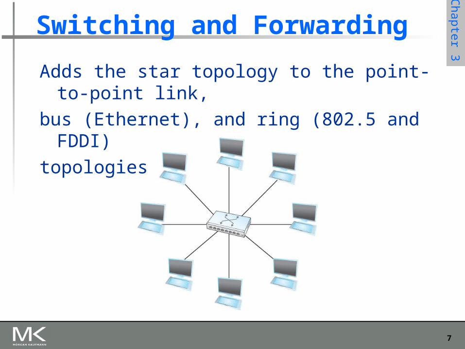
Adds the star topology to the point-to-point link,
bus (Ethernet), and ring (802.5 and FDDI)
topologies
8
Chapter 3
Chapter 3
Switching and Forwarding
Properties of this star topology Even though a switch has a fixed number of inputs and outputs,
which limits the number of hosts that can be connected to a single switch, large networks can be built by interconnecting a number of switches
We can connect switches to each other and to hosts using point-to-point links, which typically means that we can build networks of large geographic scope
Adding a new host to the network by connecting it to a switch does not necessarily mean that the hosts already connected will get worse performance from the network
9
Chapter 3
Chapter 3
Switching and Forwarding
The last claim cannot be made for the shared media network (discussed in Chapter 2) It is impossible for two hosts on the same Ethernet to
transmit continuously at 10Mbps because they share the same transmission medium
Every host on a switched network has its own link to the switch
So it may be entirely possible for many hosts to transmit at the full link speed (bandwidth) provided that the switch is designed with enough aggregate capacity
10
Chapter 3
Chapter 3
Switching and Forwarding
A switch is connected to a set of links and for each of these links, runs the appropriate data link protocol to communicate with that node
A switch’s primary job is to receive incoming packets on one of its links and to transmit them on some other link This function is referred as switching and forwarding According to OSI architecture this is the main function
of the network layer
11
Chapter 3
Chapter 3
Switching and Forwarding
How does the switch decide which output port to place each packet on? It looks at the header of the packet for an
identifier that it uses to make the decision Two common approaches
Datagram or Connectionless approach Virtual circuit or Connection-oriented approach
A third approach source routing is less common
12
Chapter 3
Chapter 3
Switching and Forwarding
Assumptions Each host has a globally unique address There is some way to identify the input and
output ports of each switch We can use numbers We can use names
13
Chapter 3
Chapter 3
Switching and Forwarding
Datagrams Key Idea
Every packet contains enough information to enable any switch to decide how to get it to destination
Every packet contains the complete destination address
14
Chapter 3
Chapter 3
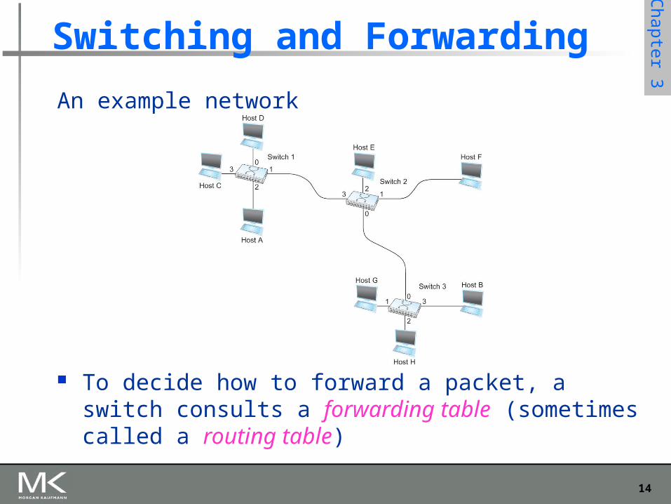
An example network
To decide how to forward a packet, a switch consults a forwarding table (sometimes called a routing table)
Switching and Forwarding
15
Chapter 3
Chapter 3
Copyright © 2010, Elsevier Inc. All rights Reserved
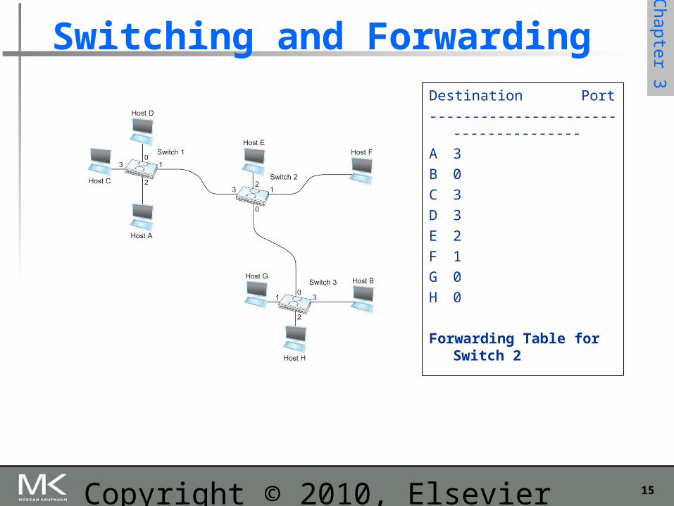
Switching and ForwardingDestination Port
-------------------------------------
A 3
B 0
C 3
D 3
E 2
F 1
G 0
H 0
Forwarding Table for Switch 2
16
Chapter 3
Chapter 3
Switching and Forwarding
Characteristics of Connectionless (Datagram) Network A host can send a packet anywhere at any time, since any
packet that turns up at the switch can be immediately forwarded (assuming a correctly populated forwarding table)
When a host sends a packet, it has no way of knowing if the network is capable of delivering it or if the destination host is even up and running
Each packet is forwarded independently of previous packets that might have been sent to the same destination.
Thus two successive packets from host A to host B may follow completely different paths
A switch or link failure might not have any serious effect on communication if it is possible to find an alternate route around the failure and update the forwarding table accordingly
17
Chapter 3
Chapter 3
Switching and Forwarding
Virtual Circuit Switching Widely used technique for packet switching Uses the concept of virtual circuit (VC) Also called a connection-oriented model First set up a virtual connection from the source host
to the destination host and then send the data
18
Chapter 3
Chapter 3
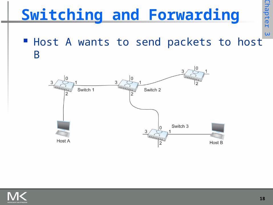
Switching and Forwarding
Host A wants to send packets to host B
19
Chapter 3
Chapter 3
Switching and Forwarding
Two-stage process Connection setup Data Transfer
Connection setup Establish “connection state” in each of the switches
between the source and destination hosts The connection state for a single connection consists
of an entry in the “VC table” in each switch through which the connection passes
20
Chapter 3
Chapter 3
Switching and Forwarding
One entry in the VC table on a single switch contains A virtual circuit identifier (VCI) that uniquely identifies the connection at
this switch and that will be carried inside the header of the packets that belong to this connection
An incoming interface on which packets for this VC arrive at the switch An outgoing interface in which packets for this VC leave the switch A potentially different VCI that will be used for outgoing packets
The semantics for one such entry is If a packet arrives on the designated incoming interface and that packet
contains the designated VCI value in its header, then the packet should be sent out the specified outgoing interface with the specified outgoing VCI value first having been placed in its header
21
Chapter 3
Chapter 3
Switching and Forwarding
Note: The combination of the VCI of the packets as they are received
at the switch and the interface on which they are received uniquely identifies the virtual connection
There may be many virtual connections established in the switch at one time
Incoming and outgoing VCI values are not generally the same VCI is not a globally significant identifier for the connection; rather it
has significance only on a given link Whenever a new connection is created, we need to assign a new
VCI for that connection on each link that the connection will traverse
We also need to ensure that the chosen VCI on a given link is not currently in use on that link by some existing connection.
22
Chapter 3
Chapter 3
Switching and Forwarding
Two broad classes of approach to establishing connection state Network Administrator will configure the state
The virtual circuit is permanent (PVC) The network administrator can delete this Can be thought of as a long-lived or administratively configured VC
A host can send messages into the network to cause the state to be established
This is referred as signalling and the resulting virtual circuit is said to be switched (SVC)
A host may set up and delete such a VC dynamically without the involvement of a network administrator
23
Chapter 3
Chapter 3
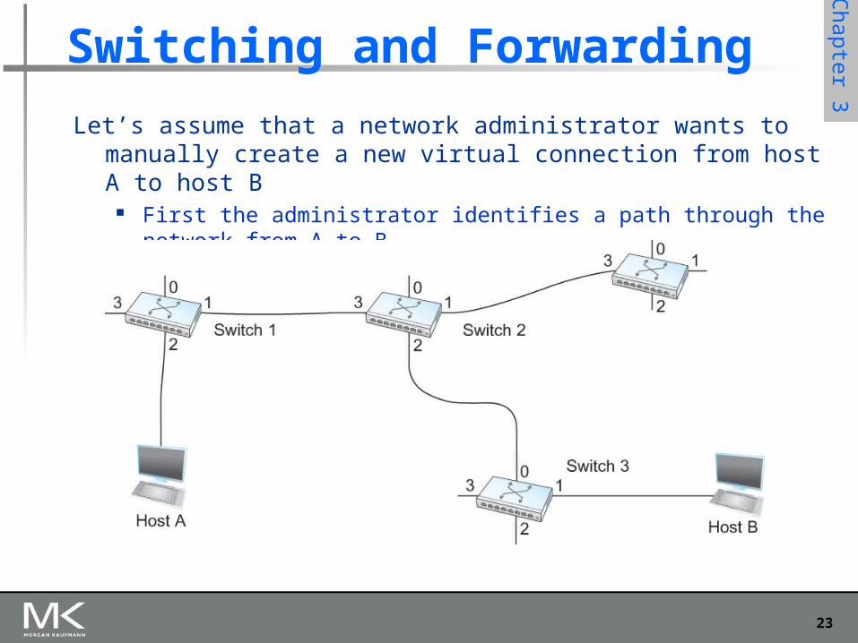
Let’s assume that a network administrator wants to manually create a new virtual connection from host A to host B
First the administrator identifies a path through the network from A to B
Switching and Forwarding
24
Chapter 3
Chapter 3
Switching and Forwarding
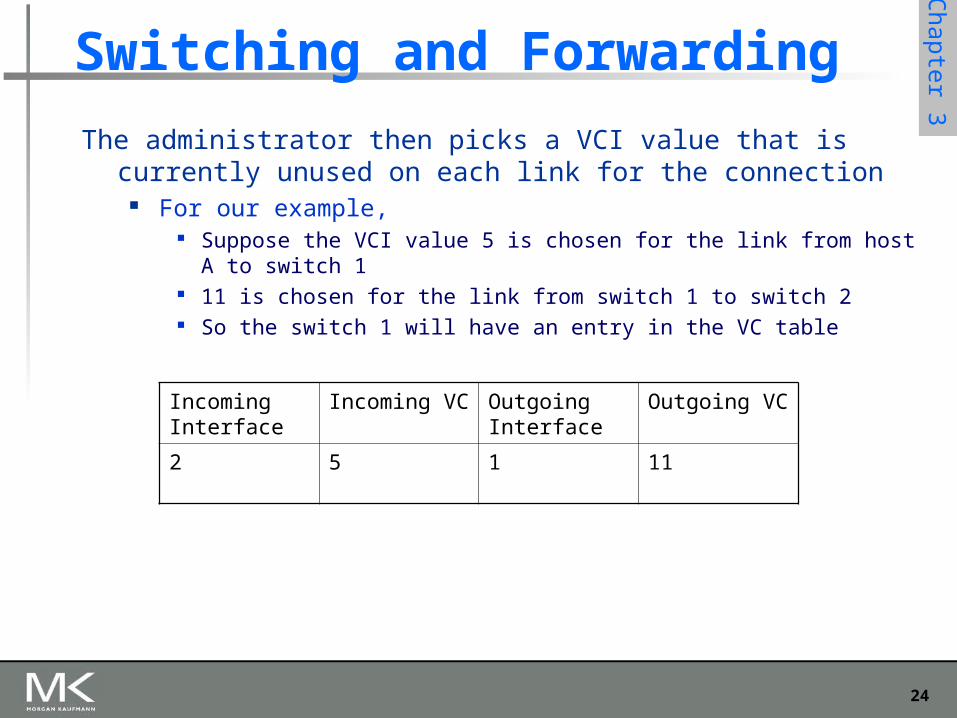
The administrator then picks a VCI value that is currently unused on each link for the connection
For our example, Suppose the VCI value 5 is chosen for the link from host A to switch 1 11 is chosen for the link from switch 1 to switch 2 So the switch 1 will have an entry in the VC table
Incoming Interface
Incoming VC Outgoing Interface
Outgoing VC
2 5 1 11
25
Chapter 3
Chapter 3
Switching and Forwarding
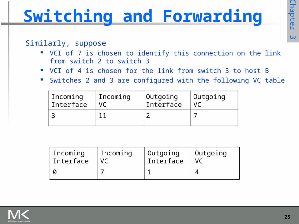
Similarly, suppose VCI of 7 is chosen to identify this connection on the link from switch 2 to switch 3 VCI of 4 is chosen for the link from switch 3 to host B Switches 2 and 3 are configured with the following VC table
Incoming Interface
Incoming VC Outgoing Interface
Outgoing VC
3 11 2 7
Incoming Interface
Incoming VC Outgoing Interface
Outgoing VC
0 7 1 4
26
Chapter 3
Chapter 3
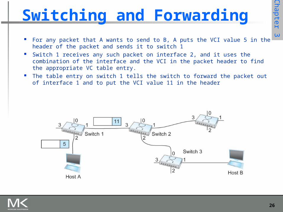
Switching and Forwarding For any packet that A wants to send to B, A puts the VCI value 5 in the header of the
packet and sends it to switch 1 Switch 1 receives any such packet on interface 2, and it uses the combination of the
interface and the VCI in the packet header to find the appropriate VC table entry. The table entry on switch 1 tells the switch to forward the packet out of interface 1
and to put the VCI value 11 in the header
27
Chapter 3
Chapter 3
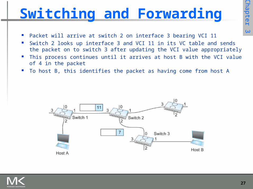
Switching and Forwarding Packet will arrive at switch 2 on interface 3 bearing VCI 11 Switch 2 looks up interface 3 and VCI 11 in its VC table and sends the packet on
to switch 3 after updating the VCI value appropriately This process continues until it arrives at host B with the VCI value of 4 in the
packet To host B, this identifies the packet as having come from host A
28
Chapter 3
Chapter 3
Switching and Forwarding In real networks of reasonable size, the burden of configuring VC tables
correctly in a large number of switches would quickly become excessive Thus, some sort of signalling is almost always used, even when setting up
“permanent” VCs In case of PVCs, signalling is initiated by the network administrator SVCs are usually set up using signalling by one of the hosts
29
Chapter 3
Chapter 3
Switching and Forwarding How does the signalling work
To start the signalling process, host A sends a setup message into the network (i.e. to switch 1) The setup message contains (among other things) the complete destination address of B. The setup message needs to get all the way to B to create the necessary connection state in every switch along the way It is like sending a datagram to B where every switch knows which output to send the setup message so that it eventually reaches B Assume that every switch knows the topology to figure out how to do that
When switch 1 receives the connection request, in addition to sending it on to switch 2, it creates a new entry in its VC table for this new connection
The entry is exactly the same shown in the previous table Switch 1 picks the value 5 for this connection
30
Chapter 3
Chapter 3
Switching and Forwarding How does the signalling work (contd.)
When switch 2 receives the setup message, it performs the similar process and it picks the value 11 as the incoming VCI Similarly switch 3 picks 7 as the value for its incoming VCI
Each switch can pick any number it likes, as long as that number is not currently in use for some other connection on that port of that switch
Finally the setup message arrives at host B. Assuming that B is healthy and willing to accept a connection from host A, it allocates an incoming VCI value, in this case
4. This VCI value can be used by B to identify all packets coming from A
31
Chapter 3
Chapter 3
Switching and Forwarding Now to complete the connection, everyone needs to be told what their downstream neighbor is using as the VCI
for this connection Host B sends an acknowledgement of the connection setup to switch 3 and includes in that message the VCI value that it
chose (4) Switch 3 completes the VC table entry for this connection and sends the acknowledgement on to switch 2 specifying the
VCI of 7 Switch 2 completes the VC table entry for this connection and sends acknowledgement on to switch 1 specifying the VCI of
11 Finally switch 1 passes the acknowledgement on to host A telling it to use the VCI value of 5 for this connection
32
Chapter 3
Chapter 3
Switching and Forwarding When host A no longer wants to send data to host B, it tears down the connection by
sending a teardown message to switch 1 The switch 1 removes the relevant entry from its table and forwards the message on
to the other switches in the path which similarly delete the appropriate table entries At this point, if host A were to send a packet with a VCI of 5 to switch 1, it would be
dropped as if the connection had never existed
33
Chapter 3
Chapter 3
Switching and Forwarding Characteristics of VC
Since host A has to wait for the connection request to reach the far side of the network and return before it can send its first data packet, there is at least one RTT of delay before data is sent
While the connection request contains the full address for host B (which might be quite large, being a global identifier on the network), each data packet contains only a small identifier, which is only unique on one link.
Thus the per-packet overhead caused by the header is reduced relative to the datagram model If a switch or a link in a connection fails, the connection is broken and a new one will need to be established.
Also the old one needs to be torn down to free up table storage space in the switches The issue of how a switch decides which link to forward the connection request on has similarities with the function of a routing algorithm
34
Chapter 3
Chapter 3
Copyright © 2010, Elsevier Inc. All rights Reserved
Switching and Forwarding Good Properties of VC
By the time the host gets the go-ahead to send data, it knows quite a lot about the network-
For example, that there is really a route to the receiver and that the receiver is willing to receive data
It is also possible to allocate resources to the virtual circuit at the time it is established
35
Chapter 3
Chapter 3
Switching and Forwarding For example, an X.25 network – a packet-switched network that
uses the connection-oriented model – employs the following three-part strategy
Buffers are allocated to each virtual circuit when the circuit is initialized The sliding window protocol is run between each pair of nodes along the
virtual circuit, and this protocol is augmented with the flow control to keep the sending node from overrunning the buffers allocated at the receiving node
The circuit is rejected by a given node if not enough buffers are available at that node when the connection request message is processed
36
Chapter 3
Chapter 3
Switching and Forwarding Comparison with the Datagram Model
Datagram network has no connection establishment phase and each switch processes each packet independently
Each arriving packet competes with all other packets for buffer space If there are no buffers, the incoming packet must be dropped
In VC, we could imagine providing each circuit with a different quality of service (QoS)
The network gives the user some kind of performance related guarantee Switches set aside the resources they need to meet this guarantee
For example, a percentage of each outgoing link’s bandwidth Delay tolerance on each switch
Most popular examples of VC technologies are Frame Relay and ATM
One of the applications of Frame Relay is the construction of VPN
37
Chapter 3
Chapter 3
Switching and Forwarding
ATM (Asynchronous Transfer Mode) Connection-oriented packet-switched network Packets are called cells
5 byte header + 48 byte payload Fixed length packets are easier to switch in
hardware Simpler to design Enables parallelism
38
Chapter 3
Chapter 3
Switching and Forwarding
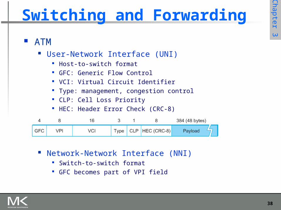
ATM User-Network Interface (UNI)
Host-to-switch format GFC: Generic Flow Control VCI: Virtual Circuit Identifier Type: management, congestion control CLP: Cell Loss Priority HEC: Header Error Check (CRC-8)
Network-Network Interface (NNI) Switch-to-switch format GFC becomes part of VPI field
39
Chapter 3
Chapter 3
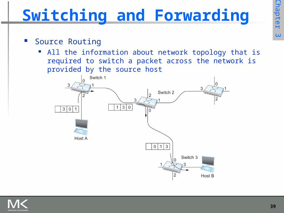
Switching and Forwarding Source Routing
All the information about network topology that is required to switch a packet across the network is provided by the source host
40
Chapter 3
Chapter 3
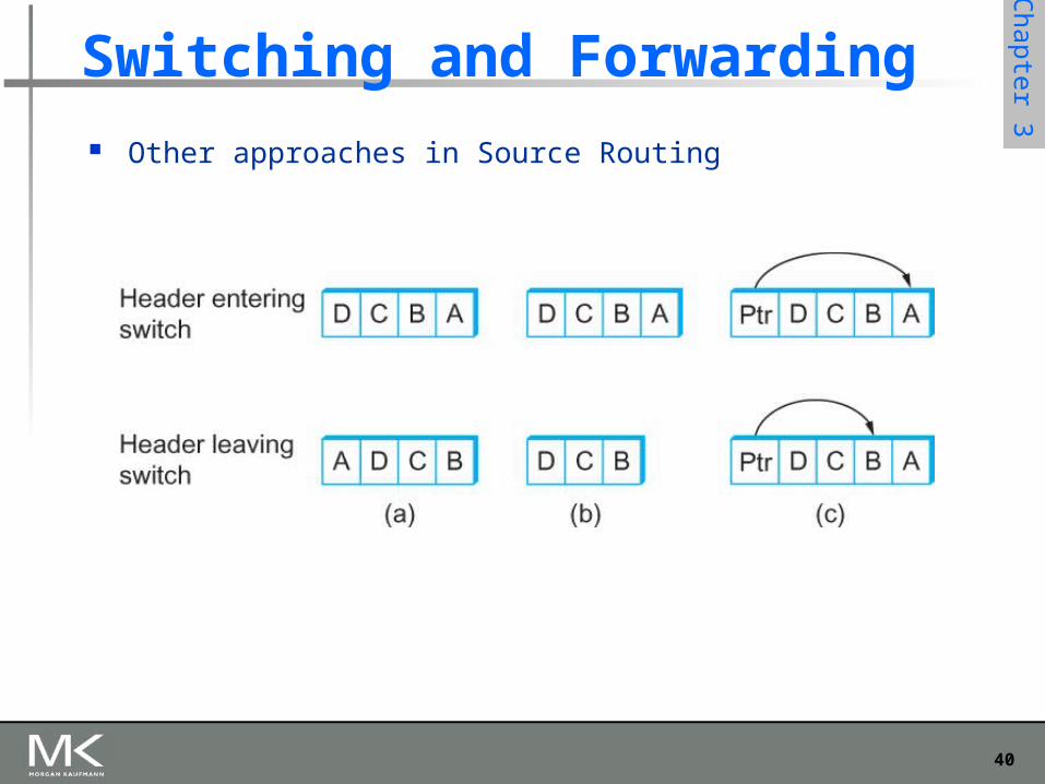
Switching and Forwarding Other approaches in Source Routing
41
Chapter 3
Chapter 3
Introduction to Congestion• Contention – The queuing of multiple
packets at an output port of a switch because they arrived at similar times. The effect is delay of the packet arriving at the output port while the port is busy.
• Congestion – The next stage of contention, where the buffers used to store contending packets are used up, requiring dropping of packets.
• See shaded box on Page 182
42
Chapter 3
Chapter 3
Optical Switching• DWDM-Dense Wavelength Division Multiplexing
• Multiple wavelengths(colors) on single fiber
• ex: 100 channels of 10Gbps each
• Optical Amplifiers
• Old repeater spacing (back to electric) ~ 40Km
• DWDM equipment required at each repeater
• With Amplifiers 100’s of Km possible
• Optical Switches
• Current technology electrically ‘forward’ SONET channels
• Emerging technology using micro-mirror manipulation
• See shaded box on page 183
43
Chapter 3
Chapter 3
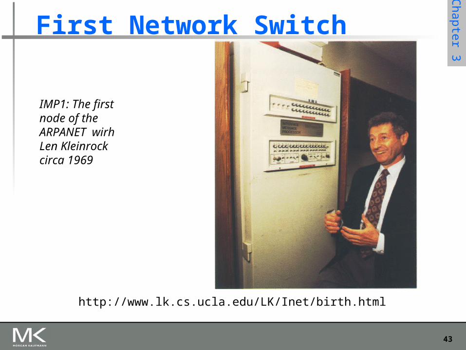
First Network Switch
IMP1: The first node of the ARPANET wirh Len Kleinrock circa 1969
http://www.lk.cs.ucla.edu/LK/Inet/birth.html
44
Chapter 3
Chapter 3
Bridges and LAN Switches Bridges and LAN Switches
Class of switches that is used to forward packets between shared-media LANs such as Ethernets
Known as LAN switches Referred to as Bridges
Suppose you have a pair of Ethernets that you want to interconnect One approach is put a repeater in between them
It might exceed the physical limitation of the Ethernet No more than four repeaters between any pair of hosts No more than a total of 2500 m in length is allowed
An alternative would be to put a node between the two Ethernets and have the node forward frames from one Ethernet to the other
This node is called a Bridge A collection of LANs connected by one or more bridges is usually said to form an
Extended LAN
45
Chapter 3
Chapter 3
Bridges and LAN Switches Simplest Strategy for Bridges
Accept LAN frames on their inputs and forward them out to all other outputs
Used by early bridges
Learning Bridges Observe that there is no need to forward all the frames that a bridge
receives
46
Chapter 3
Chapter 3
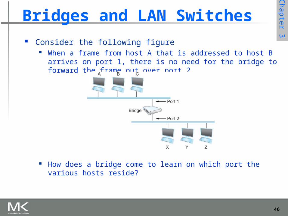
Consider the following figure When a frame from host A that is addressed to host B arrives on port 1,
there is no need for the bridge to forward the frame out over port 2.
How does a bridge come to learn on which port the various hosts reside?
Bridges and LAN Switches
47
Chapter 3
Chapter 3
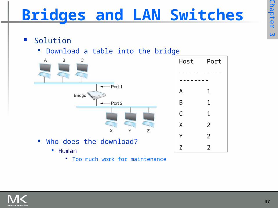
Bridges and LAN Switches Solution
Download a table into the bridge
Who does the download? Human
Too much work for maintenance
A
Bridge
B C
X Y Z
Port 1
Port 2
Host Port
--------------------
A 1
B 1
C 1
X 2
Y 2
Z 2
48
Chapter 3
Chapter 3
Bridges and LAN Switches Can the bridge learn this information by itself?
Yes
How Each bridge inspects the source address in all the frames it receives Record the information at the bridge and build the table When a bridge first boots, this table is empty Entries are added over time A timeout is associated with each entry The bridge discards the entry after a specified period of time
To protect against the situation in which a host is moved from one network to another
If the bridge receives a frame that is addressed to host not currently in the table
Forward the frame out on all other ports
49
Chapter 3
Chapter 3
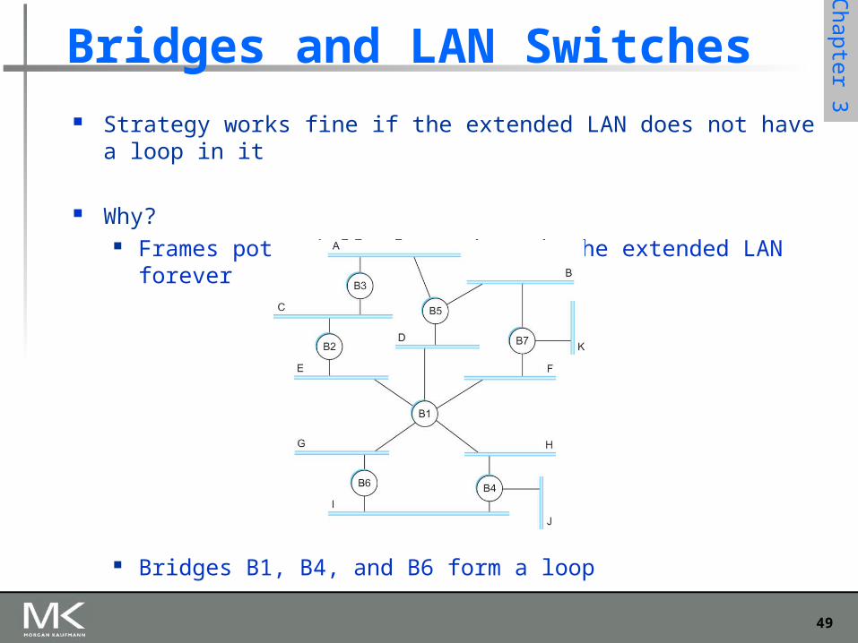
Bridges and LAN Switches Strategy works fine if the extended LAN does not have a loop in it
Why? Frames potentially loop through the extended LAN forever
Bridges B1, B4, and B6 form a loop
50
Chapter 3
Chapter 3
Bridges and LAN Switches How does an extended LAN come to have a loop in it?
Network is managed by more than one administrator For example, it spans multiple departments in an organization It is possible that no single person knows the entire configuration of
the network A bridge that closes a loop might be added without anyone knowing
Loops are built into the network to provide redundancy in case of failures
Solution Distributed Spanning Tree Algorithm
51
Chapter 3
Chapter 3
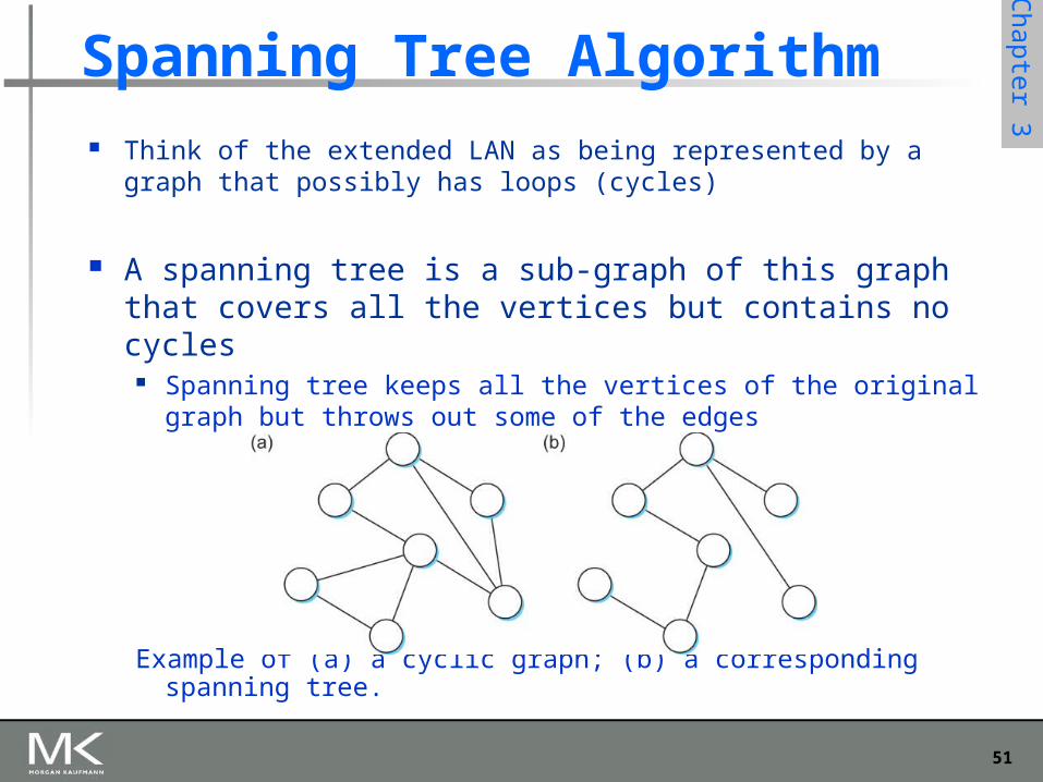
Spanning Tree Algorithm Think of the extended LAN as being represented by a graph that
possibly has loops (cycles)
A spanning tree is a sub-graph of this graph that covers all the vertices but contains no cycles
Spanning tree keeps all the vertices of the original graph but throws out some of the edges
Example of (a) a cyclic graph; (b) a corresponding spanning tree.
52
Chapter 3
Chapter 3
Spanning Tree Algorithm Developed by Radia Perlman at Digital
A protocol used by a set of bridges to agree upon a spanning tree for a particular extended LAN
IEEE 802.1 specification for LAN bridges is based on this algorithm
Each bridge decides the ports over which it is and is not willing to forward frames
In a sense, it is by removing ports from the topology that the extended LAN is reduced to an acyclic tree
It is even possible that an entire bridge will not participate in forwarding frames
53
Chapter 3
Chapter 3
Spanning Tree Algorithm Algorithm is dynamic
The bridges are always prepared to reconfigure themselves into a new spanning tree if some bridges fail
Main idea Each bridge selects the ports over which they will forward the
frames
54
Chapter 3
Chapter 3
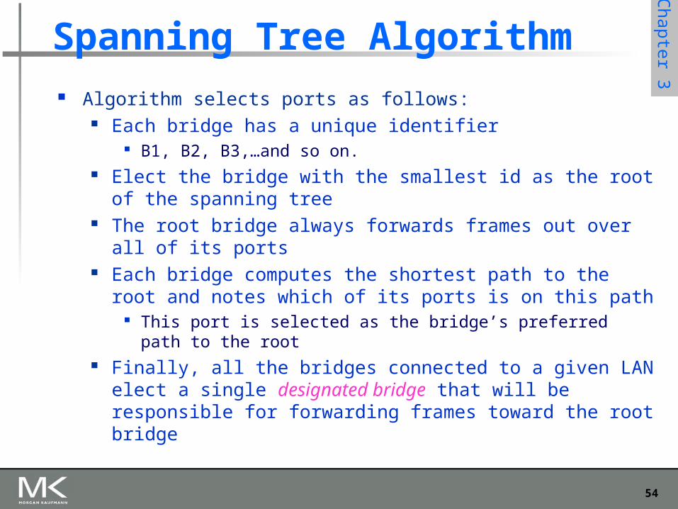
Spanning Tree Algorithm Algorithm selects ports as follows:
Each bridge has a unique identifier B1, B2, B3,…and so on.
Elect the bridge with the smallest id as the root of the spanning tree
The root bridge always forwards frames out over all of its ports Each bridge computes the shortest path to the root and notes
which of its ports is on this path This port is selected as the bridge’s preferred path to the root
Finally, all the bridges connected to a given LAN elect a single designated bridge that will be responsible for forwarding frames toward the root bridge
55
Chapter 3
Chapter 3
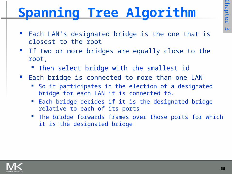
Spanning Tree Algorithm Each LAN’s designated bridge is the one that is closest to the root If two or more bridges are equally close to the root,
Then select bridge with the smallest id Each bridge is connected to more than one LAN
So it participates in the election of a designated bridge for each LAN it is connected to.
Each bridge decides if it is the designated bridge relative to each of its ports
The bridge forwards frames over those ports for which it is the designated bridge
56
Chapter 3
Chapter 3
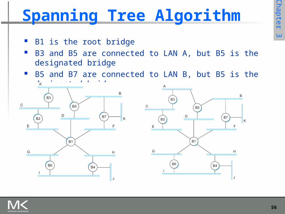
Spanning Tree Algorithm B1 is the root bridge B3 and B5 are connected to LAN A, but B5 is the designated bridge B5 and B7 are connected to LAN B, but B5 is the designated bridge
57
Chapter 3
Chapter 3
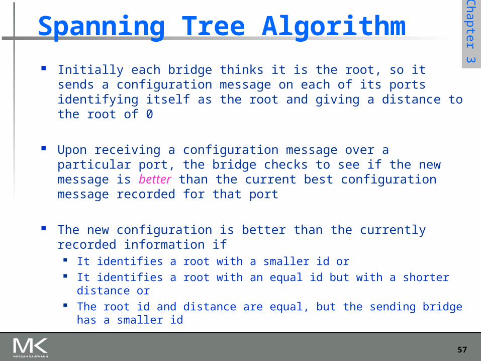
Spanning Tree Algorithm Initially each bridge thinks it is the root, so it sends a configuration
message on each of its ports identifying itself as the root and giving a distance to the root of 0
Upon receiving a configuration message over a particular port, the bridge checks to see if the new message is better than the current best configuration message recorded for that port
The new configuration is better than the currently recorded information if
It identifies a root with a smaller id or It identifies a root with an equal id but with a shorter distance or The root id and distance are equal, but the sending bridge has a smaller
id
58
Chapter 3
Chapter 3
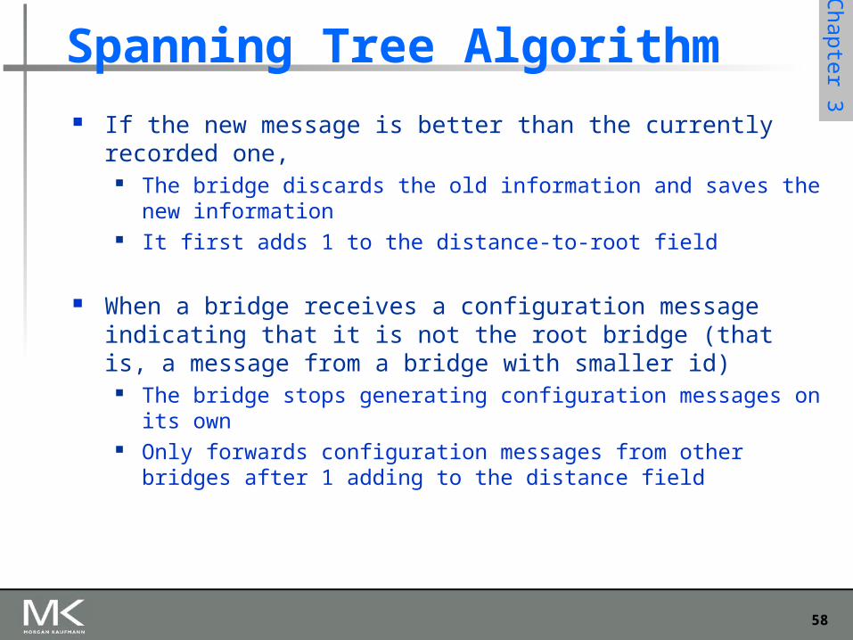
Spanning Tree Algorithm If the new message is better than the currently recorded one,
The bridge discards the old information and saves the new information It first adds 1 to the distance-to-root field
When a bridge receives a configuration message indicating that it is not the root bridge (that is, a message from a bridge with smaller id)
The bridge stops generating configuration messages on its own Only forwards configuration messages from other bridges after 1 adding
to the distance field
59
Chapter 3
Chapter 3
Spanning Tree Algorithm
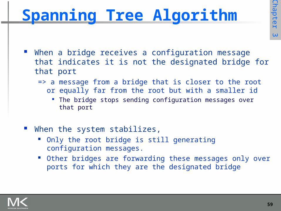
When a bridge receives a configuration message that indicates it is not the designated bridge for that port => a message from a bridge that is closer to the root or equally far from the
root but with a smaller id The bridge stops sending configuration messages over that port
When the system stabilizes, Only the root bridge is still generating configuration messages. Other bridges are forwarding these messages only over ports for which
they are the designated bridge
60
Chapter 3
Chapter 3
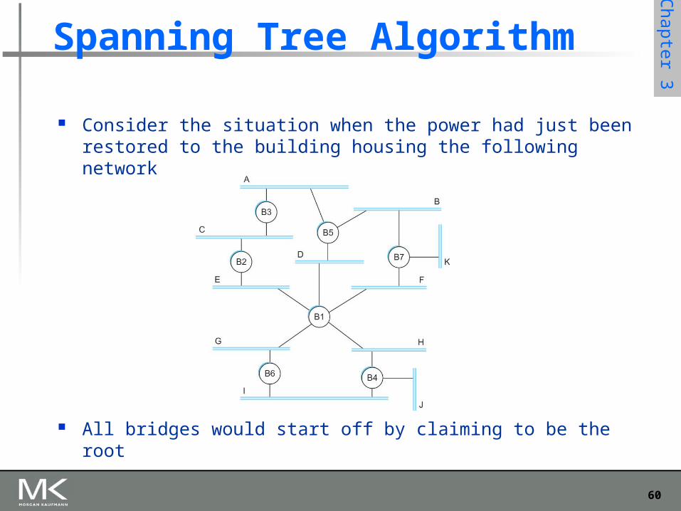
Spanning Tree Algorithm
Consider the situation when the power had just been restored to the building housing the following network
All bridges would start off by claiming to be the root
61
Chapter 3
Chapter 3
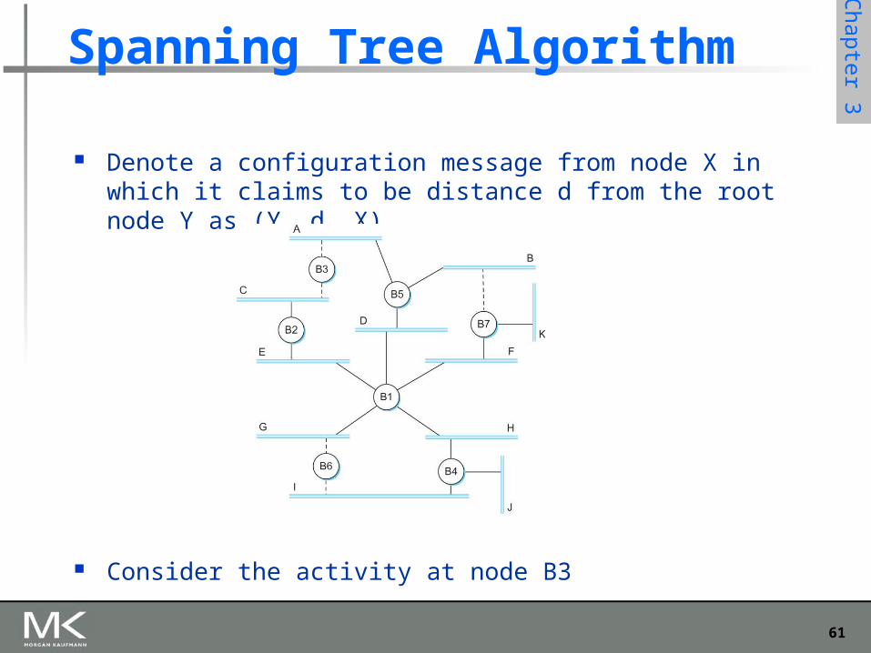
Spanning Tree Algorithm
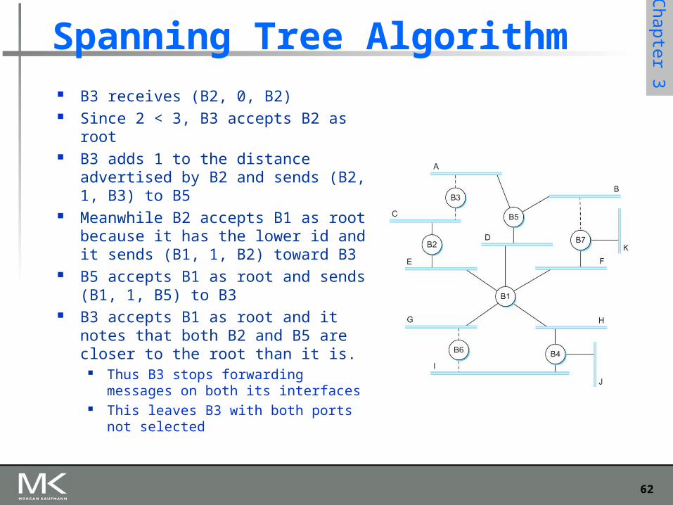
Denote a configuration message from node X in which it claims to be distance d from the root node Y as (Y, d, X)
Consider the activity at node B3
62
Chapter 3
Chapter 3
Spanning Tree Algorithm B3 receives (B2, 0, B2) Since 2 < 3, B3 accepts B2 as root B3 adds 1 to the distance advertised
by B2 and sends (B2, 1, B3) to B5 Meanwhile B2 accepts B1 as root
because it has the lower id and it sends (B1, 1, B2) toward B3
B5 accepts B1 as root and sends (B1, 1, B5) to B3
B3 accepts B1 as root and it notes that both B2 and B5 are closer to the root than it is.
Thus B3 stops forwarding messages on both its interfaces
This leaves B3 with both ports not selected
63
Chapter 3
Chapter 3
Spanning Tree Algorithm Even after the system has stabilized, the root bridge continues to
send configuration messages periodically Other bridges continue to forward these messages
When a bridge fails, the downstream bridges will not receive the configuration messages
After waiting a specified period of time, they will once again claim to be the root and the algorithm starts again
Note Although the algorithm is able to reconfigure the spanning tree whenever
a bridge fails, it is not able to forward frames over alternative paths for the sake of routing around a congested bridge
64
Chapter 3
Chapter 3
Spanning Tree Algorithm
Broadcast and Multicast Forward all broadcast/multicast frames
Current practice Learn when no group members downstream Accomplished by having each member of
group G send a frame to bridge multicast address with G in source field
65
Chapter 3
Chapter 3
Spanning Tree Algorithm
Limitation of Bridges Do not scale
Spanning tree algorithm does not scale Broadcast does not scale
Do not accommodate heterogeneity Caution: Beware of Transparency
66
Chapter 3
Chapter 3
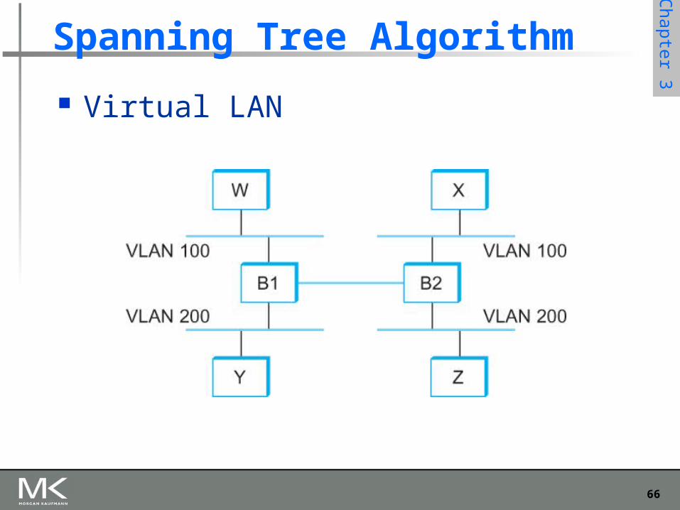
Spanning Tree Algorithm
Virtual LAN
67
Chapter 3
Chapter 3
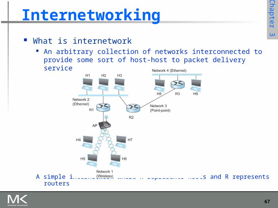
Internetworking
What is internetwork An arbitrary collection of networks interconnected to provide
some sort of host-host to packet delivery service
A simple internetwork where H represents hosts and R represents routers
68
Chapter 3
Chapter 3
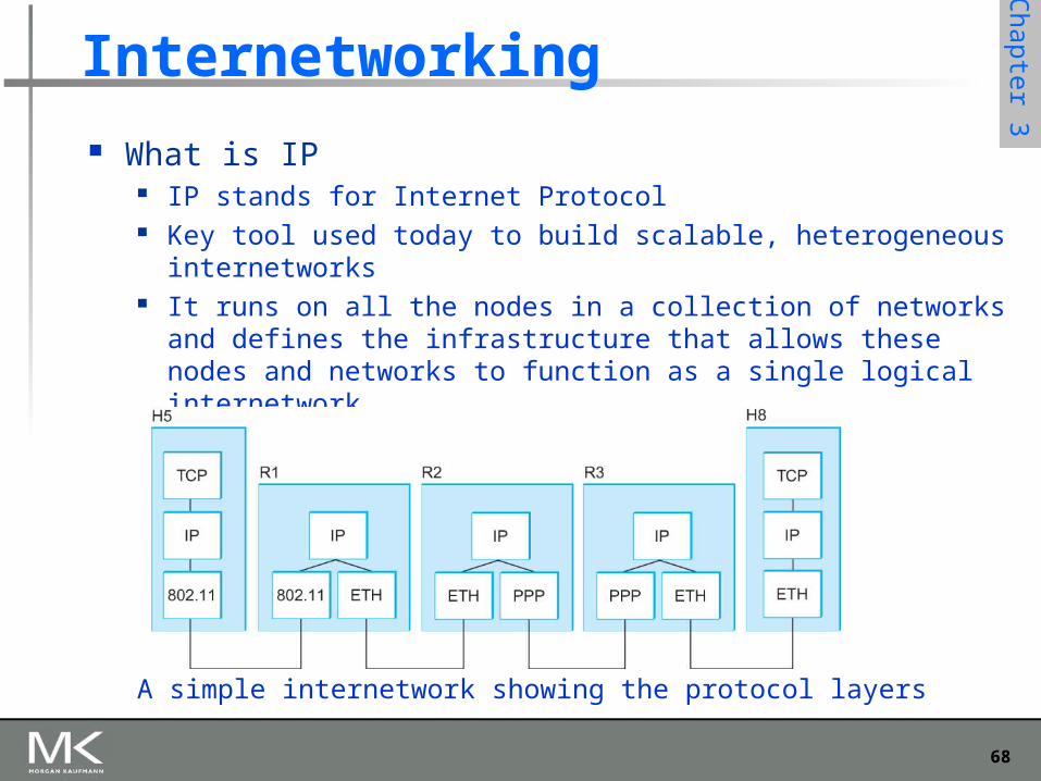
Internetworking
What is IP IP stands for Internet Protocol Key tool used today to build scalable, heterogeneous
internetworks It runs on all the nodes in a collection of networks and defines
the infrastructure that allows these nodes and networks to function as a single logical internetwork
A simple internetwork showing the protocol layers
69
Chapter 3
Chapter 3
IP Service Model
Packet Delivery Model Connectionless model for data delivery Best-effort delivery (unreliable service)
packets are lost packets are delivered out of order duplicate copies of a packet are delivered packets can be delayed for a long time
Global Addressing Scheme Provides a way to identify all hosts in the network
70
Chapter 3
Chapter 3
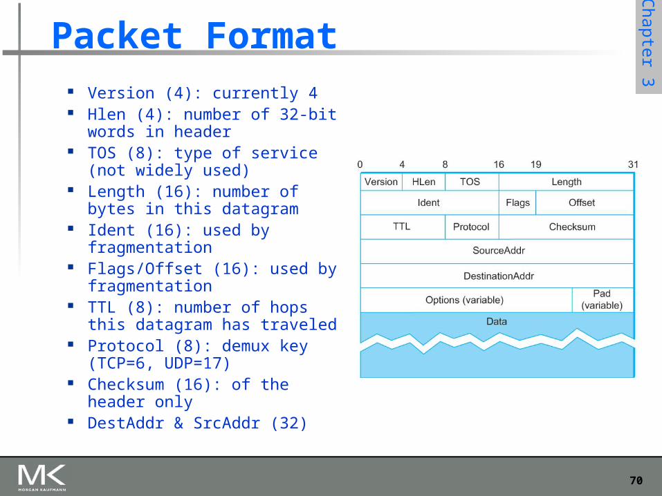
Packet Format Version (4): currently 4 Hlen (4): number of 32-bit words
in header TOS (8): type of service (not
widely used) Length (16): number of bytes in
this datagram Ident (16): used by fragmentation Flags/Offset (16): used by
fragmentation TTL (8): number of hops this
datagram has traveled Protocol (8): demux key (TCP=6,
UDP=17) Checksum (16): of the header
only DestAddr & SrcAddr (32)
71
Chapter 3
Chapter 3
IP Fragmentation and Reassembly
Each network has some MTU (Maximum Transmission Unit) Ethernet (1500 bytes), FDDI (4500 bytes)
Strategy Fragmentation occurs in a router when it receives a
datagram that it wants to forward over a network which has (MTU < datagram)
Reassembly is done at the receiving host All the fragments carry the same identifier in the Ident
field Fragments are self-contained datagrams IP does not recover from missing fragments
72
Chapter 3
Chapter 3
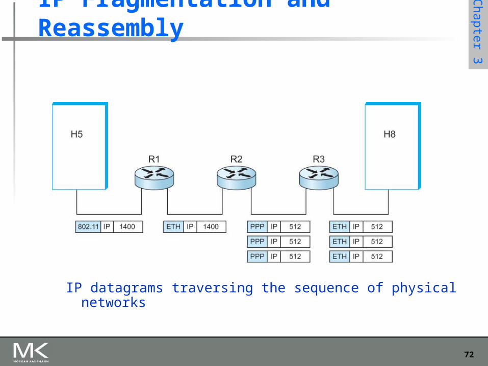
IP Fragmentation and Reassembly
IP datagrams traversing the sequence of physical networks
73
Chapter 3
Chapter 3
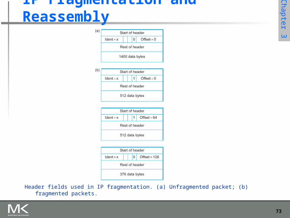
IP Fragmentation and Reassembly
Header fields used in IP fragmentation. (a) Unfragmented packet; (b) fragmented packets.
74
Chapter 3
Chapter 3
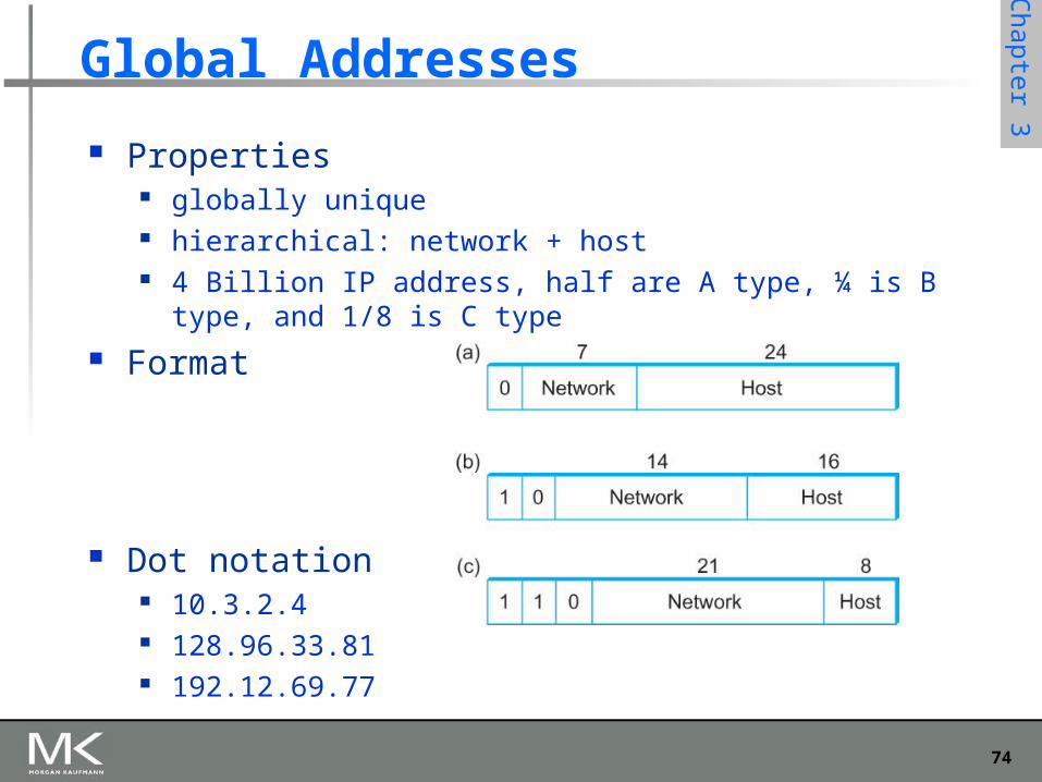
Global Addresses
Properties globally unique hierarchical: network + host 4 Billion IP address, half are A type, ¼ is B type, and 1/8 is C
type Format
Dot notation 10.3.2.4 128.96.33.81 192.12.69.77
75
Chapter 3
Chapter 3
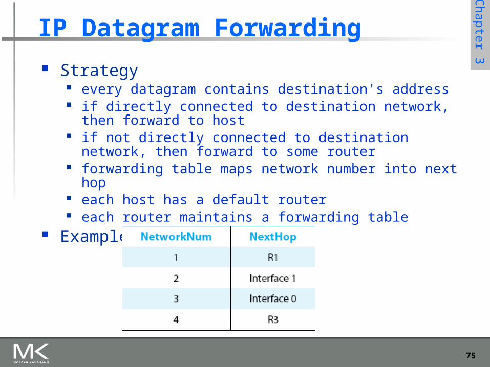
IP Datagram Forwarding
Strategy every datagram contains destination's address if directly connected to destination network, then forward to host if not directly connected to destination network, then forward to
some router forwarding table maps network number into next hop each host has a default router each router maintains a forwarding table
Example (router R2)
76
Chapter 3
Chapter 3
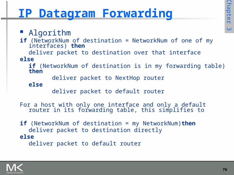
IP Datagram Forwarding Algorithmif (NetworkNum of destination = NetworkNum of one of my
interfaces) thendeliver packet to destination over that interface
elseif (NetworkNum of destination is in my forwarding table) then
deliver packet to NextHop routerelse
deliver packet to default router
For a host with only one interface and only a default router in its forwarding table, this simplifies to
if (NetworkNum of destination = my NetworkNum)thendeliver packet to destination directly
elsedeliver packet to default router
77
Chapter 3
Chapter 3
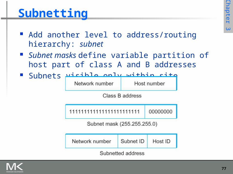
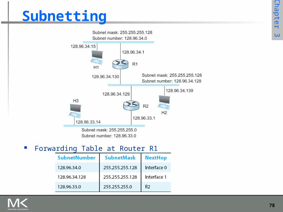
Subnetting
Add another level to address/routing hierarchy: subnet Subnet masks define variable partition of host part of
class A and B addresses Subnets visible only within site
78
Chapter 3
Chapter 3
Subnetting
Forwarding Table at Router R1
79
Chapter 3
Chapter 3
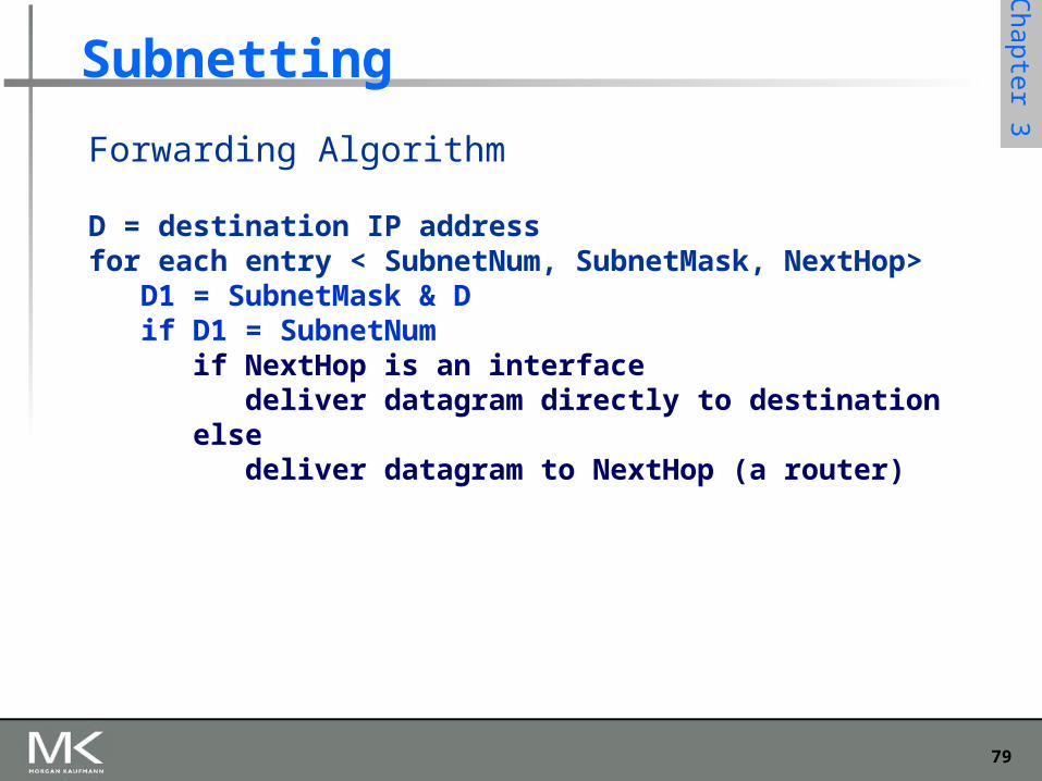
Subnetting
Forwarding Algorithm
D = destination IP addressfor each entry < SubnetNum, SubnetMask, NextHop>
D1 = SubnetMask & Dif D1 = SubnetNum
if NextHop is an interface deliver datagram directly to destinationelse deliver datagram to NextHop (a router)
80
Chapter 3
Chapter 3
Subnetting
Notes Would use a default router if nothing matches Not necessary for all ones in subnet mask to be
contiguous Can put multiple subnets on one physical network Subnets not visible from the rest of the Internet
81
Chapter 3
Chapter 3
Classless Addressing
Classless Inter-Domain Routing A technique that addresses two scaling concerns in
the Internet The growth of backbone routing table as more and more
network numbers need to be stored in them Potential exhaustion of the 32-bit address space
Address assignment efficiency Arises because of the IP address structure with class A, B,
and C addresses Forces us to hand out network address space in fixed-size
chunks of three very different sizes A network with two hosts needs a class C address
Address assignment efficiency = 2/255 = 0.78 A network with 256 hosts needs a class B address
Address assignment efficiency = 256/65535 = 0.39
82
Chapter 3
Chapter 3
Classless Addressing
Exhaustion of IP address space centers on exhaustion of the class B network numbers
Solution Say “NO” to any Autonomous System (AS) that requests a class
B address unless they can show a need for something close to 64K addresses
Instead give them an appropriate number of class C addresses For any AS with at least 256 hosts, we can guarantee an address
space utilization of at least 50% What is the problem with this solution?
83
Chapter 3
Chapter 3
Classless Addressing
Problem with this solution Excessive storage requirement at the routers.
If a single AS has, say 16 class C network numbers assigned to it, Every Internet backbone router needs 16 entries in its
routing tables for that AS This is true, even if the path to every one of these
networks is the same If we had assigned a class B address to the AS
The same routing information can be stored in one entry
Efficiency = 16 × 255 / 65, 536 = 6.2%
84
Chapter 3
Chapter 3
Classless Addressing
CIDR tries to balance the desire to minimize the number of routes that a router needs to know against the need to hand out addresses efficiently.
CIDR uses aggregate routes Uses a single entry in the forwarding table to tell the
router how to reach a lot of different networks Breaks the rigid boundaries between address classes
85
Chapter 3
Chapter 3
Classless Addressing
Consider an AS with 16 class C network numbers. Instead of handing out 16 addresses at random, hand
out a block of contiguous class C addresses Suppose we assign the class C network numbers from
192.4.16 through 192.4.31 Observe that top 20 bits of all the addresses in this range
are the same (11000000 00000100 0001) We have created a 20-bit network number (which is in between
class B network number and class C number) Requires to hand out blocks of class C addresses that
share a common prefix
86
Chapter 3
Chapter 3
Classless Addressing
Requires to hand out blocks of class C addresses that share a common prefix
The convention is to place a /X after the prefix where X is the prefix length in bits
For example, the 20-bit prefix for all the networks 192.4.16 through 192.4.31 is represented as 192.4.16/20
By contrast, if we wanted to represent a single class C network number, which is 24 bits long, we would write it 192.4.16/24
87
Chapter 3
Chapter 3
Classless Addressing
How do the routing protocols handle this classless addresses It must understand that the network number may be of
any length Represent network number with a single pair
<length, value>
All routers must understand CIDR addressing
88
Chapter 3
Chapter 3
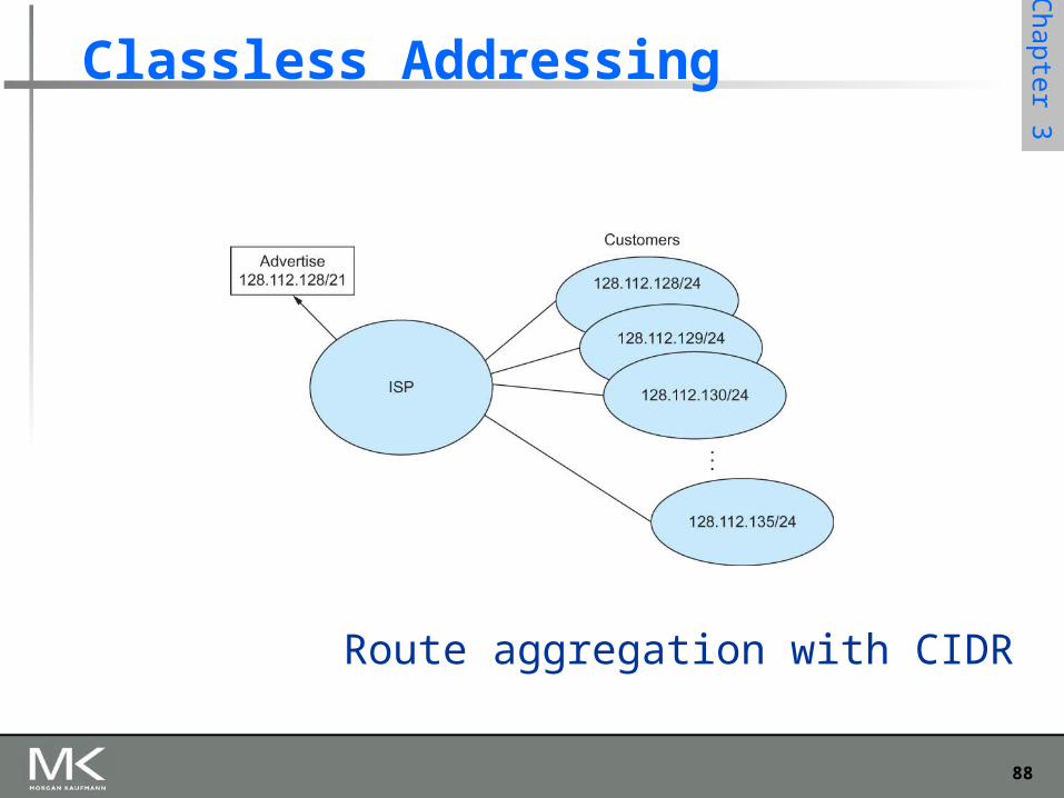
Classless Addressing
Route aggregation with CIDR
89
Chapter 3
Chapter 3
IP Forwarding Revisited
IP forwarding mechanism assumes that it can find the network number in a packet and then look up that number in the forwarding table
We need to change this assumption in case of CIDR
CIDR means that prefixes may be of any length, from 2 to 32 bits
90
Chapter 3
Chapter 3
IP Forwarding Revisited
It is also possible to have prefixes in the forwarding tables that overlap
Some addresses may match more than one prefix
For example, we might find both 171.69 (a 16 bit prefix) and 171.69.10 (a 24 bit prefix) in the forwarding table of a single router
A packet destined to 171.69.10.5 clearly matches both prefixes.
The rule is based on the principle of “longest match” 171.69.10 in this case
A packet destined to 171.69.20.5 would match 171.69 and not 171.69.10
91
Chapter 3
Chapter 3
Address Translation Protocol (ARP)
Map IP addresses into physical addresses destination host next hop router
Techniques encode physical address in host part of IP address table-based
ARP (Address Resolution Protocol) table of IP to physical address bindings broadcast request if IP address not in table target machine responds with its physical address table entries are discarded if not refreshed
92
Chapter 3
Chapter 3
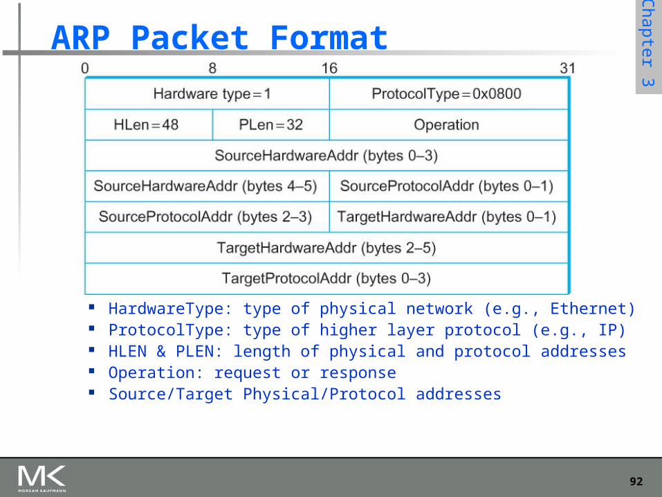
ARP Packet Format
HardwareType: type of physical network (e.g., Ethernet) ProtocolType: type of higher layer protocol (e.g., IP) HLEN & PLEN: length of physical and protocol addresses Operation: request or response Source/Target Physical/Protocol addresses
93
Chapter 3
Chapter 3
Host Configurations
Notes Ethernet addresses are configured into network by
manufacturer and they are unique IP addresses must be unique on a given internetwork
but also must reflect the structure of the internetwork Most host Operating Systems provide a way to
manually configure the IP information for the host Drawbacks of manual configuration
A lot of work to configure all the hosts in a large network Configuration process is error-prune
Automated Configuration Process is required
94
Chapter 3
Chapter 3
Dynamic Host Configuration Protocol (DHCP)
DHCP server is responsible for providing configuration information to hosts
There is at least one DHCP server for an administrative domain
DHCP server maintains a pool of available addresses
95
Chapter 3
Chapter 3
DHCP
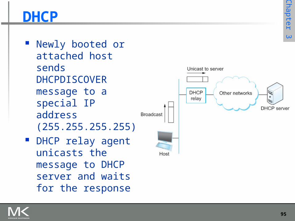
Newly booted or attached host sends DHCPDISCOVER message to a special IP address (255.255.255.255)
DHCP relay agent unicasts the message to DHCP server and waits for the response
96
Chapter 3
Chapter 3
Internet Control Message Protocol (ICMP)
Defines a collection of error messages that are sent back to the source host whenever a router or host is unable to process an IP datagram successfully
Destination host unreachable due to link /node failure Reassembly process failed TTL had reached 0 (so datagrams don't cycle forever) IP header checksum failed
ICMP-Redirect From router to a source host With a better route information
97
Chapter 3
Chapter 3
Routing
Forwarding versus Routing– Forwarding:
– to select an output port based on destination address and routing table
– Routing: – process by which routing table is built
98
Chapter 3
Chapter 3
Routing
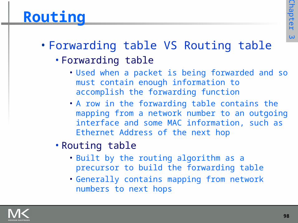
• Forwarding table VS Routing table• Forwarding table
• Used when a packet is being forwarded and so must contain enough information to accomplish the forwarding function
• A row in the forwarding table contains the mapping from a network number to an outgoing interface and some MAC information, such as Ethernet Address of the next hop
• Routing table • Built by the routing algorithm as a precursor to build the
forwarding table• Generally contains mapping from network numbers to
next hops
99
Chapter 3
Chapter 3
Routing
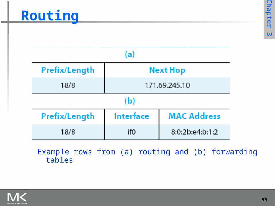
Example rows from (a) routing and (b) forwarding tables
100
Chapter 3
Chapter 3
Routing
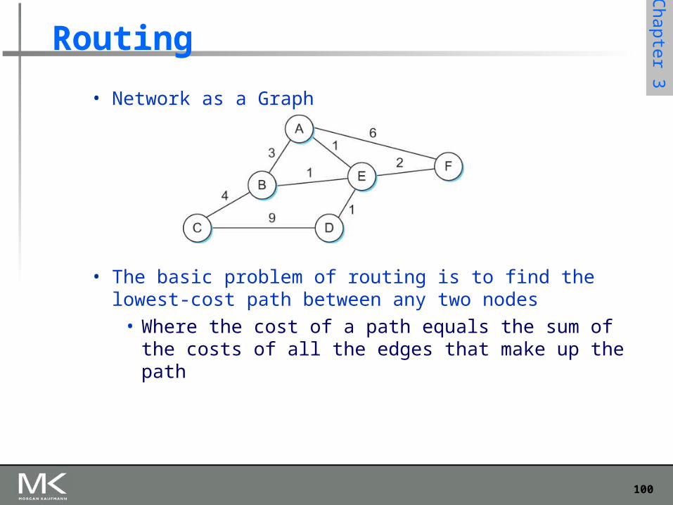
• Network as a Graph
• The basic problem of routing is to find the lowest-cost path between any two nodes
• Where the cost of a path equals the sum of the costs of all the edges that make up the path
101
Chapter 3
Chapter 3
Routing
• For a simple network, we can calculate all shortest paths and load them into some nonvolatile storage on each node.
• Such a static approach has several shortcomings• It does not deal with node or link failures• It does not consider the addition of new nodes or links• It implies that edge costs cannot change
• What is the solution?• Need a distributed and dynamic protocol• Two main classes of protocols
• Distance Vector• Link State
102
Chapter 3
Chapter 3
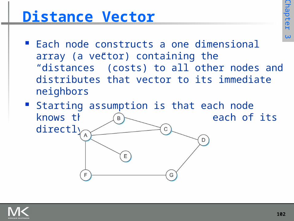
Distance Vector
Each node constructs a one dimensional array (a vector) containing the “distances” (costs) to all other nodes and distributes that vector to its immediate neighbors
Starting assumption is that each node knows the cost of the link to each of its directly connected neighbors
103
Chapter 3
Chapter 3
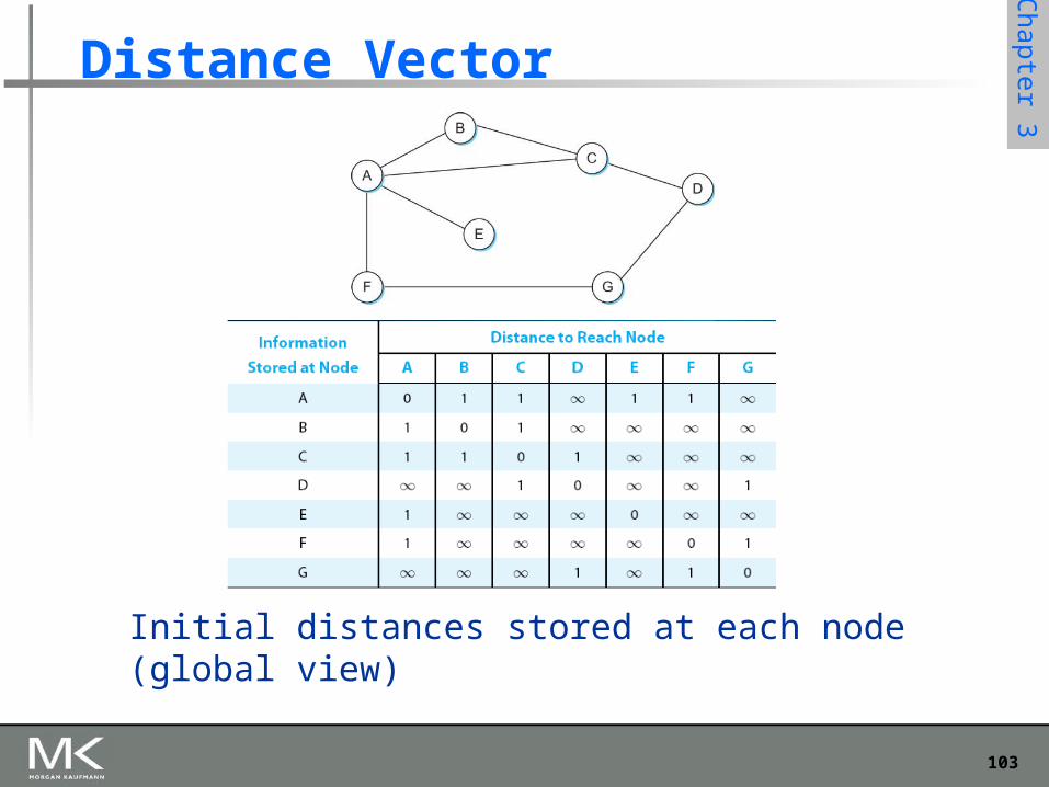
Distance Vector
Initial distances stored at each node (global view)
104
Chapter 3
Chapter 3
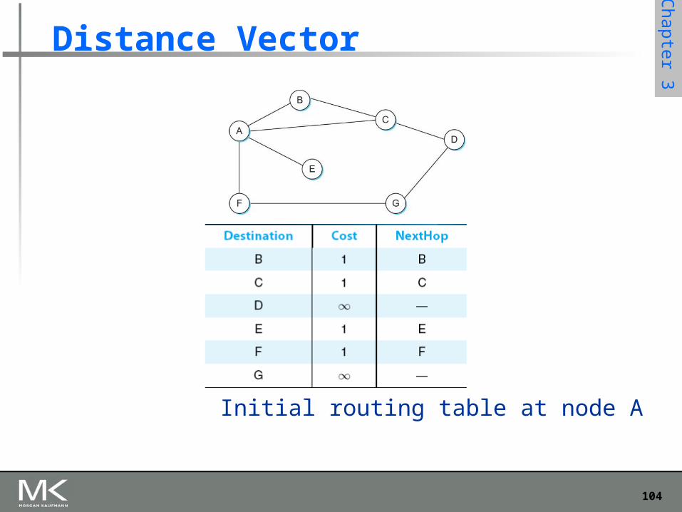
Distance Vector
Initial routing table at node A
105
Chapter 3
Chapter 3
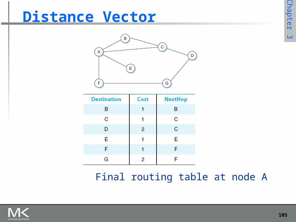
Distance Vector
Final routing table at node A
106
Chapter 3
Chapter 3
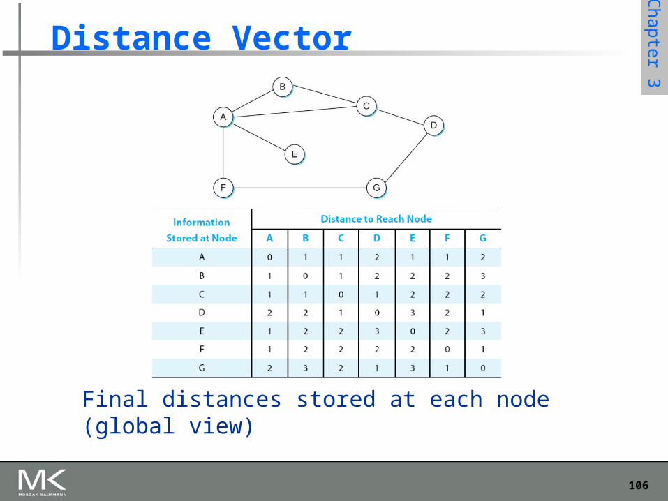
Distance Vector
Final distances stored at each node (global view)
107
Chapter 3
Chapter 3
Distance Vector
The distance vector routing algorithm is sometimes called as Bellman-Ford algorithm
Every T seconds each router sends its table to its neighbor each each router then updates its table based on the new information
Problems include fast response to good new and slow response to bad news. Also too many messages to update
108
Chapter 3
Chapter 3
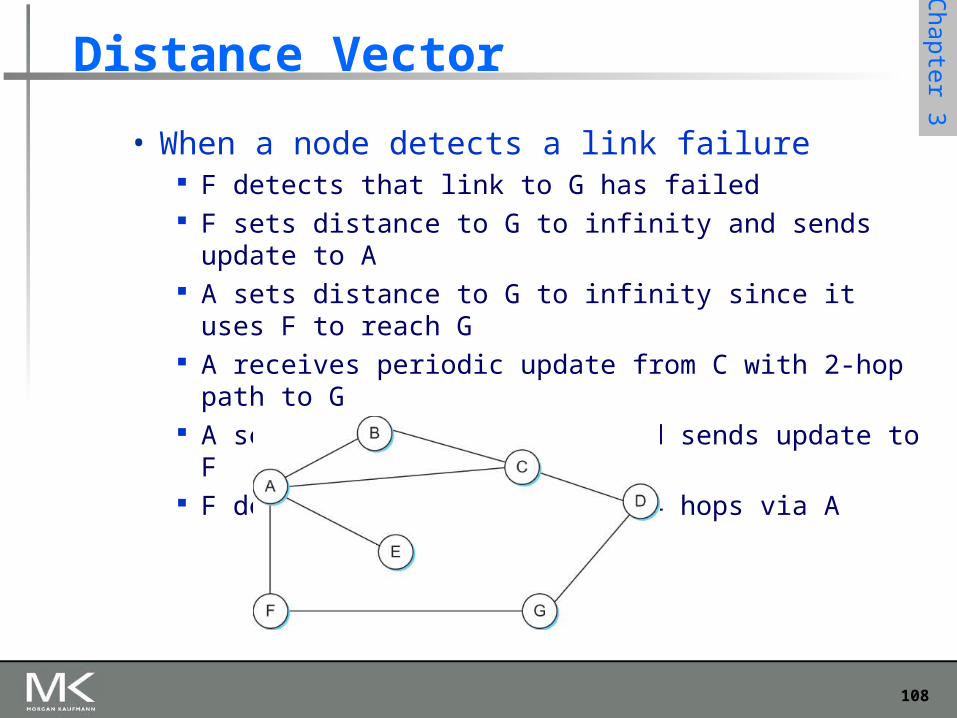
Distance Vector
• When a node detects a link failure F detects that link to G has failed F sets distance to G to infinity and sends update to A A sets distance to G to infinity since it uses F to reach G A receives periodic update from C with 2-hop path to G A sets distance to G to 3 and sends update to F F decides it can reach G in 4 hops via A
109
Chapter 3
Chapter 3
Distance Vector
Slightly different circumstances can prevent the network from stabilizing
Suppose the link from A to E goes down In the next round of updates, A advertises a distance of infinity to E, but
B and C advertise a distance of 2 to E Depending on the exact timing of events, the following might happen
Node B, upon hearing that E can be reached in 2 hops from C, concludes that it can reach E in 3 hops and advertises this to A
Node A concludes that it can reach E in 4 hops and advertises this to C Node C concludes that it can reach E in 5 hops; and so on. This cycle stops only when the distances reach some number that is large
enough to be considered infinite Count-to-infinity problem
110
Chapter 3
Chapter 3
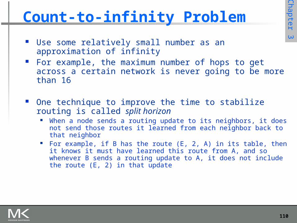
Count-to-infinity Problem
Use some relatively small number as an approximation of infinity For example, the maximum number of hops to get across a certain
network is never going to be more than 16
One technique to improve the time to stabilize routing is called split horizon
When a node sends a routing update to its neighbors, it does not send those routes it learned from each neighbor back to that neighbor
For example, if B has the route (E, 2, A) in its table, then it knows it must have learned this route from A, and so whenever B sends a routing update to A, it does not include the route (E, 2) in that update
111
Chapter 3
Chapter 3
Count-to-infinity Problem
In a stronger version of split horizon, called split horizon with poison reverse
B actually sends that back route to A, but it puts negative information in the route to ensure that A will not eventually use B to get to E
For example, B sends the route (E, ∞) to A
112
Chapter 3
Chapter 3
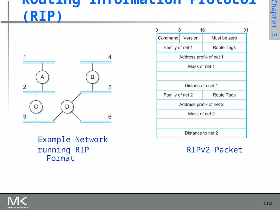
Routing Information Protocol (RIP)
Example Networkrunning RIP RIPv2 Packet Format
113
Chapter 3
Chapter 3
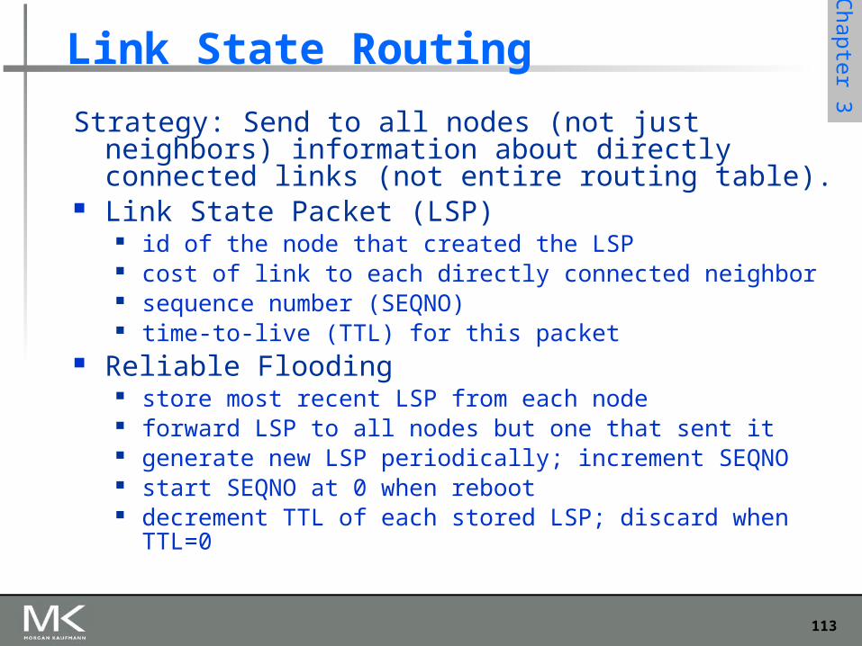
Link State Routing
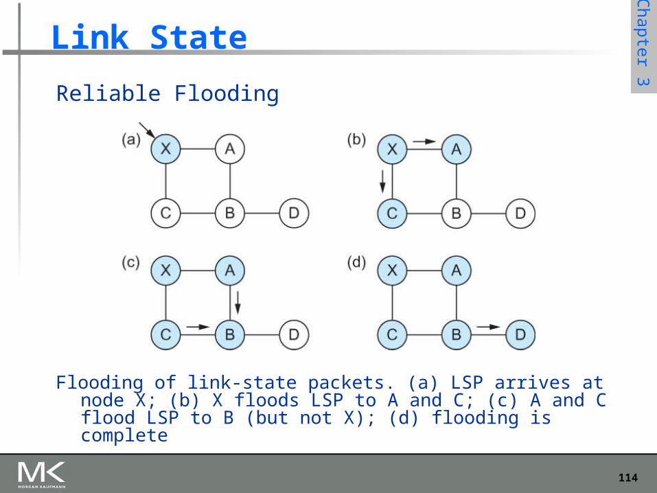
Strategy: Send to all nodes (not just neighbors) information about directly connected links (not entire routing table).
Link State Packet (LSP) id of the node that created the LSP cost of link to each directly connected neighbor sequence number (SEQNO) time-to-live (TTL) for this packet
Reliable Flooding store most recent LSP from each node forward LSP to all nodes but one that sent it generate new LSP periodically; increment SEQNO start SEQNO at 0 when reboot decrement TTL of each stored LSP; discard when TTL=0
114
Chapter 3
Chapter 3
Link State
Reliable Flooding
Flooding of link-state packets. (a) LSP arrives at node X; (b) X floods LSP to A and C; (c) A and C flood LSP to B (but not X); (d) flooding is complete
115
Chapter 3
Chapter 3
Shortest Path Routing
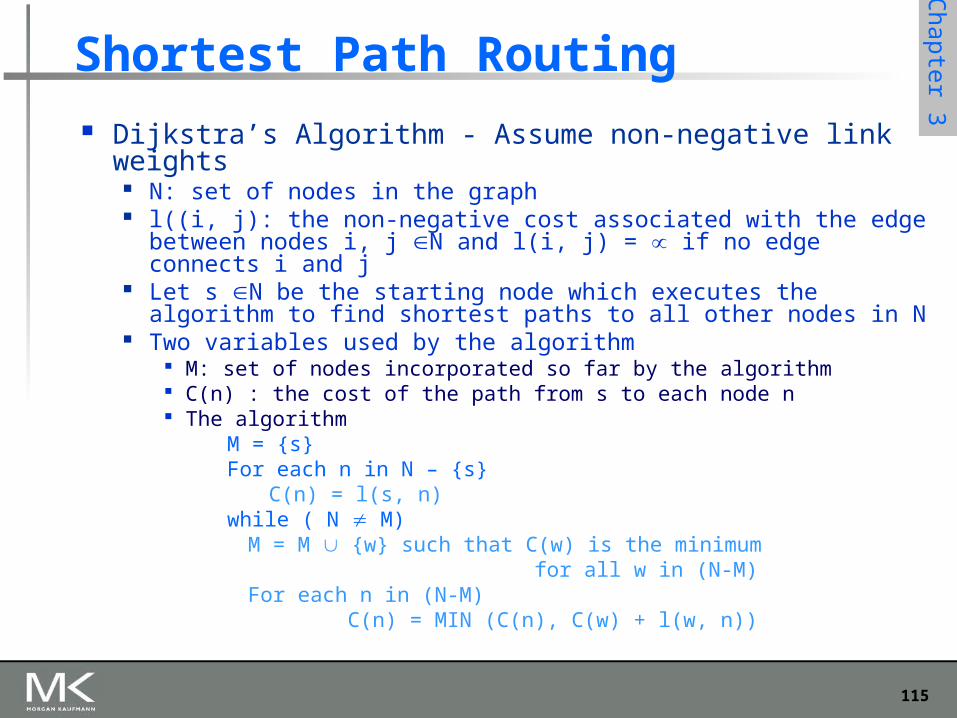
Dijkstra’s Algorithm - Assume non-negative link weights N: set of nodes in the graph l((i, j): the non-negative cost associated with the edge between
nodes i, j N and l(i, j) = if no edge connects i and j Let s N be the starting node which executes the algorithm to
find shortest paths to all other nodes in N Two variables used by the algorithm
M: set of nodes incorporated so far by the algorithm C(n) : the cost of the path from s to each node n The algorithm
M = {s}For each n in N – {s}
C(n) = l(s, n)while ( N M)M = M {w} such that C(w) is the minimum for all w in (N-M)For each n in (N-M) C(n) = MIN (C(n), C(w) + l(w, n))
116
Chapter 3
Chapter 3
Shortest Path Routing
In practice, each switch computes its routing table directly from the LSP’s it has collected using a realization of Dijkstra’s algorithm called the forward search algorithm
Specifically each switch maintains two lists, known as Tentative and Confirmed
Each of these lists contains a set of entries of the form (Destination, Cost, NextHop)
# Chapter S
ubtitle
117
Chapter 3
Chapter 3
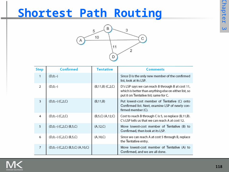
Shortest Path Routing
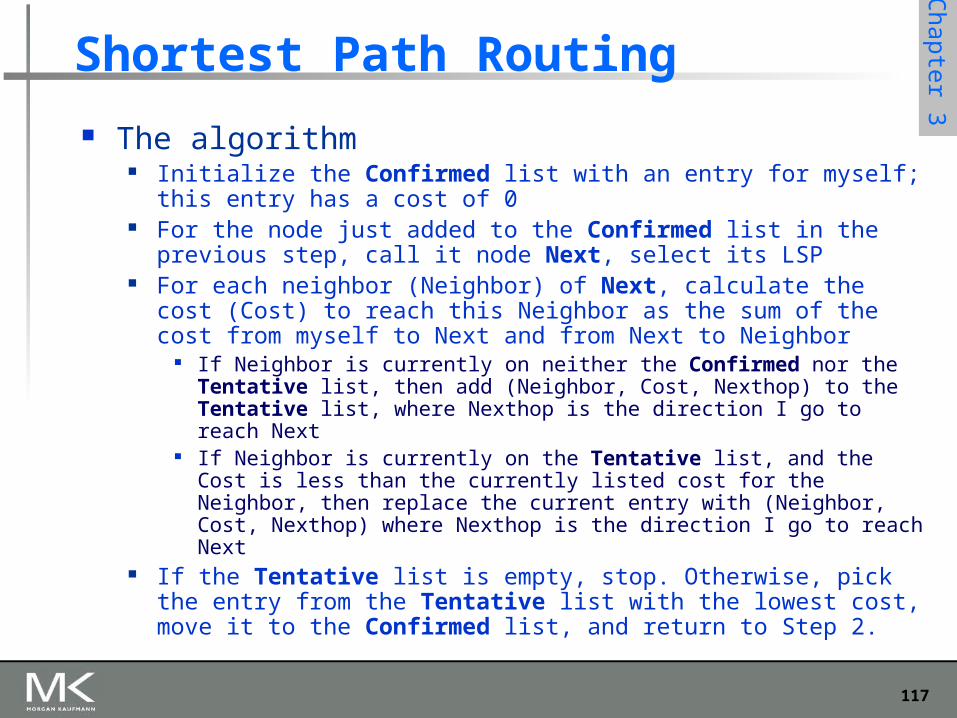
The algorithm Initialize the Confirmed list with an entry for myself; this entry has a cost
of 0 For the node just added to the Confirmed list in the previous step, call it
node Next, select its LSP For each neighbor (Neighbor) of Next, calculate the cost (Cost) to reach
this Neighbor as the sum of the cost from myself to Next and from Next to Neighbor
If Neighbor is currently on neither the Confirmed nor the Tentative list, then add (Neighbor, Cost, Nexthop) to the Tentative list, where Nexthop is the direction I go to reach Next
If Neighbor is currently on the Tentative list, and the Cost is less than the currently listed cost for the Neighbor, then replace the current entry with (Neighbor, Cost, Nexthop) where Nexthop is the direction I go to reach Next
If the Tentative list is empty, stop. Otherwise, pick the entry from the Tentative list with the lowest cost, move it to the Confirmed list, and return to Step 2.
118
Chapter 3
Chapter 3
Shortest Path Routing
119
Chapter 3
Chapter 3
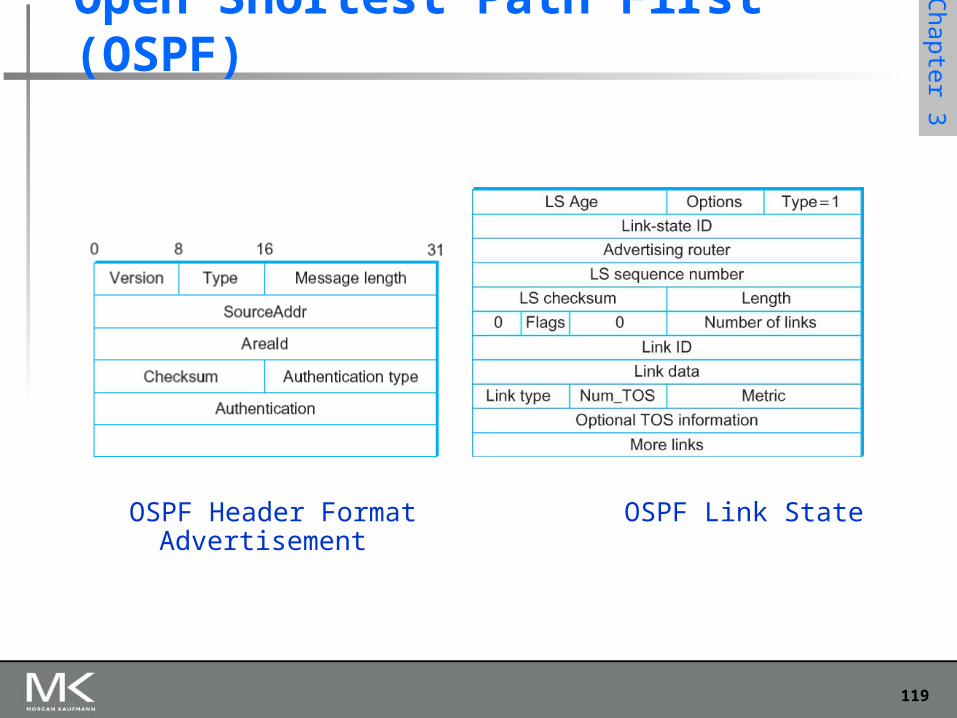
Open Shortest Path First (OSPF)
OSPF Header Format OSPF Link State Advertisement
120
Chapter 3
Chapter 3
Summary
We have looked at some of the issues involved in building scalable and heterogeneous networks by using switches and routers to interconnect links and networks.
To deal with heterogeneous networks, we have discussed in details the service model of Internetworking Protocol (IP) which forms the basis of today’s routers.
We have discussed in details two major classes of routing algorithms
Distance Vector Link State