Unit 3

UNIT-3

Points to be covered:

(A) Test of H:ypothesis-I

• Introduction and procedure

• Null and alternative hypothesis

• Simple and composite hypothesis

• Sample error, level of significance, one and two tail.

(B) Test of Hypothesis-II

• Difference between large and small sample test

• Degree of freedom

• Condition for applying T-Test.

(C )Application of T-Test:

• Test of significance of mean

• Test of significance of difference of two mean

• Paired T-Test

(D) Large Sample test (Z test):

• Test of significance of mean

• Test of significance of difference of two mean,

• Test of significance between two S.D.

(A)Testing of Hypothesis-1

Introduction:

The main objective of taking a sample from a population is to get reliable information about the population.

From the information obtained from the sample, conclusions are drawn about the population.

This is called statistical inference.

It may consist of two parts:

(1) Estimation of parameters

(2) Test of statistical hypothesis

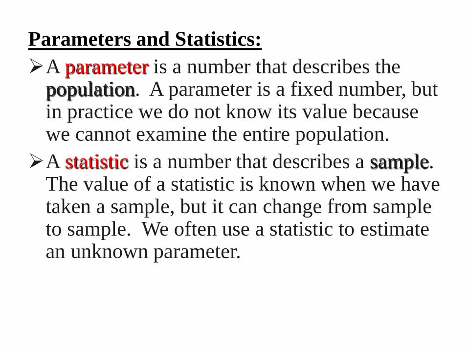
Parameters and Statistics:

A parameter is a number that describes the population. A parameter is a fixed number, but in practice we do not know its value because we cannot examine the entire population.

A statistic is a number that describes a sample. The value of a statistic is known when we have taken a sample, but it can change from sample to sample. We often use a statistic to estimate an unknown parameter.

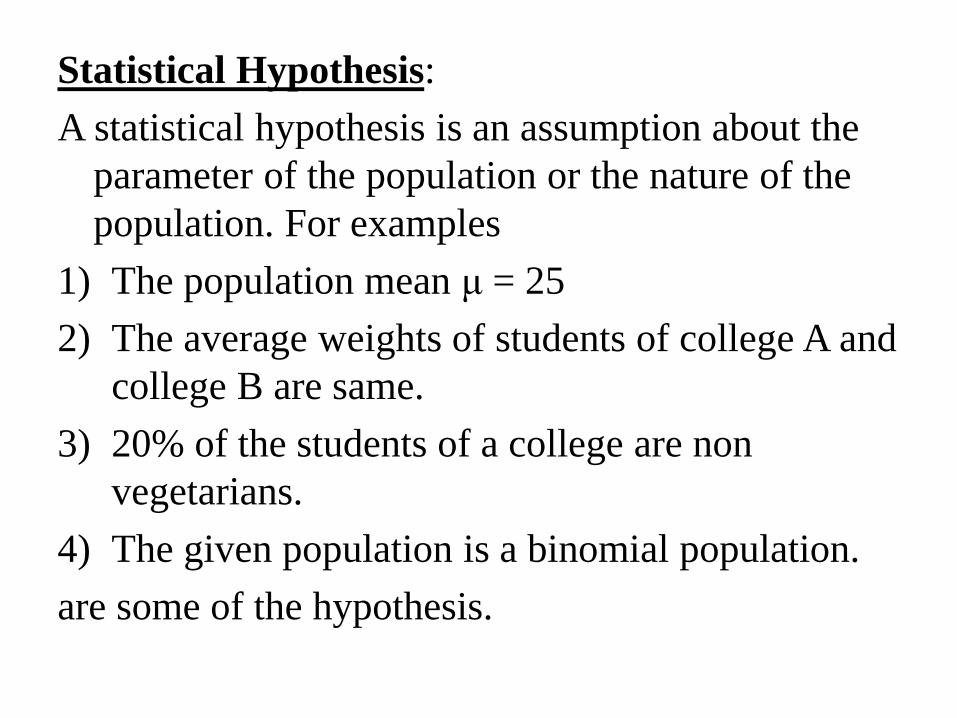
Statistical Hypothesis:

A statistical hypothesis is an assumption about the

parameter of the population or the nature of the

population. For examples

1) The population mean μ = 25

2) The average weights of students of college A and

college B are same.

3) 20% of the students of a college are non

vegetarians.

4) The given population is a binomial population.

are some of the hypothesis.

Null Hypothesis:

A statistical hypothesis which is taken for the possible acceptance is called a null hypothesis and it is denoted by H0

The neutral attitude of the decision maker, before the sample observations are taken is the key note of the null hypothesis.

For examples:

1) Mean of the population is 60. H0 : μ = 60.

2) Means of both populations are equal. H0 : μ1 = : μ2

3) The proportion of drinkers in both the cities are equal

H0 : P1 = P2

Alternative Hypothesis:

A hypothesis is complementary to the null

hypothesis is called alternative hypothesis and

it is denoted by H1.

For examples:

(1)H1: μ ≠ 60

(2)H1 : μ1 ≠ μ2

(3)H1: P1 ≠ P2

are alternative hypothesis.

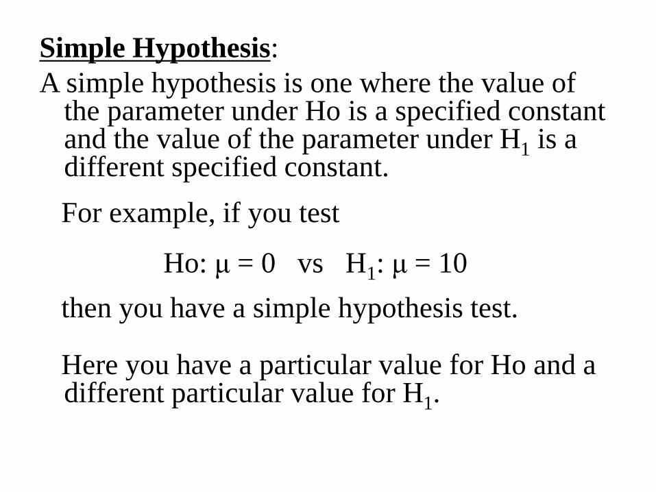
Simple Hypothesis:

A simple hypothesis is one where the value of the parameter under Ho is a specified constant and the value of the parameter under H1 is a different specified constant.

For example, if you test

Ho: μ = 0 vs H1: μ = 10

then you have a simple hypothesis test.

Here you have a particular value for Ho and a different particular value for H1.

Composite Hypothesis:

Most problems involve more than a single alternative. Such hypotheses are called composite hypotheses.

Examples of composite hypotheses:

Ho: μ = 0 vs H1: μ ≠ 0

which is a two-sided H1.

A one-sided H1 can be written as

Ho: μ = 0 vs H1: μ > 0

or

Ho: μ = 0 vs H1: μ < 0

All of these hypotheses are composite because they include more than one value for H1.

Sample Error (standard Error):

The standard deviation of the sample statistic is called standard error of the statistics.

For example, if different samples of the same size n are drawn from a population, we get different values of sample mean (x-bar).

The S.D. of (x-bar) is called standard error of (x-bar).

Standard error of (x-bar) will depend upon the size of the sample and the variability of the population.

It can be derived that S.E. = (σ / √n).

Standard errors of some well known statistics:

NO. STATISTICS S.E

1. Mean (x-bar)

2. Difference between two means

3. Sample Proportion p

4. Difference between two

proportions

P1’ – p2’

n

1 2x x2 2

1 2

1 2n n

PQ

n

1 1 2 2

1 2

PQ PQ

n n

Uses of S.E:

1) To test whether a given value of a statistic differs significantly from the intended population parameter. i.e. whether the difference between value of the sample statistic and population parameter is significant and the difference may be attribute to chance.

2) To test the randomness of a sample i.e. to test whether the given sample be regarded as a random sample from the population.

3) To obtain confidence interval for the parameter of the population.

4) To determine the precision of the sample estimate, because precision of a statistic

= 1/ S.E. of the statistic

Type I and type II Errors:

In testing of a statistical hypothesis the following situations

may arise:

1) The hypothesis may be true but it is rejected by the test.

2) The hypothesis may be false but it is accepted by the test.

3) The hypothesis may be true and is accepted by the test.

4) The hypothesis may be false and is rejected by the test.

(3) and (4) are the correct decisions while (1) and (2) are

errors.

The error committed in rejecting a hypothesis which is true

is called Type-I error and its probability is denoted by α

The error committed in accepting a hypothesis which is

false is called Type-II error and its probability is denoted by

β.

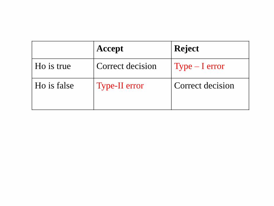
Accept Reject

Ho is true Correct decision Type – I error

Ho is false Type-II error Correct decision

Level of Significance:

In any test procedure both the types of errors should be kept minimum.

They are inter-related it is not possible to minimize both the errors simultaneously.

Hence in practice, the probability of type-I error is fixed and type –II error is minimized.

The fixed value of type-I error is called level of significance and it is denoted by α.

Thus level of significance is the probability of rejecting a hypothesis might to be accepted.

Most commonly used l.o.s. are 5% and 1%.

When decision is taken at 5% l.o.s., it means that in 5 cases out of 100, it is likely to reject a hypothesis which might to be accepted.

i.e. our decision to reject Ho is 95% correct.

Critical Region:

If test statistic falls in some interval which

support alternative hypothesis, we reject the null

hypothesis. This interval is called rejection region

It test statistic falls in some interval which support

null hypothesis, we fail to reject the alternative

hypothesis. This interval is called acceptance

region

The value of the point, which divide the rejection

region and acceptance one is called critical value

24 - 19

One-Sided or One-Tailed Hypothesis Tests

In most applications, a two-sided or two-tailed

hypothesis test is the most appropriate approach. This

approach is based on the expression of the null and

alternative hypotheses as follows:

H0: = 170 vs H1: ≠ 170

To test the above hypothesis, we set up the rejection

and acceptance regions as shown on the next slide,

where we are using = 0.05.

Reject H0

0.025

Reject H0

0.025

Accept H0

Z

0.95

In this example, the rejection region probabilities

are equally split between the two tails, thus the

reason for the label as a two-tailed test.

This procedure allows the possibility of rejecting

the null hypothesis, but does not specifically

address, in the sense of statistical significance,

the direction of the difference detected.

There may be situations when it would be

appropriate to consider an alternative hypothesis

where the directionality is specifically addressed.

That is we may want to be able to select between

a null hypothesis and one that explicitly goes in

one direction. Such a hypothesis test can best be

expressed as:

H0: = 170 vs H1: > 170

The expression is sometimes given as:

H0: ≤ 170 vs H1: > 170

The difference between the two has to do with how

the null hypothesis is expressed and the implication

of this expression.

The first expression above is the more theoretically

correct one and carries with it the clear connotation

that an outcome in the opposite direction of the

alternative hypothesis is not considered possible.

This is, in fact, the way the test is actually done.

The process of testing the above hypothesis is identical to that for the two-tailed test except that all the rejection region probabilities are in one tail.

For a test, with α = 0.05, the acceptance region would be, for example, the area from the extreme left up to the point below which lies 95% of the area.

The rejection region would be the 5% area in the upper tail.

24 - 25

Critical values at important level of significance

are given below.

1% 5% 10%

Two tailed test 2.58 1.96 1.645

One tailed test 2.33 1.645 1.282

(B) Testing Of Hypothesis -2:

Introduction:

• The value of a statistics obtained from a large sample is generally close to the parameter of the population.

• But there are situations when one has to take a small sample. E.g. if a new medicine is to be introduced, a doctor cannot test the new medicine by giving it to many patients.

• Thus he takes a small sample.

• Generally a sample having number of observations less than or equal to 30 is regarded as a small sample.

Difference between Large and Small sample

Sr. No. Large sample Small sample

1. The sample size is greater than 30. The sample size is 30 or less than 30

2. The value of a statistic obtain from the sample can be taken as an estimate of the population parameter.

The value of a statistic obtain from the sample can not be taken as an estimate of the population parameter.

3. Normal distribution is used for testing.

Sampling distribution like t, F etc. are used for testing.

Degree of freedom:

• Degree of freedom is the number of independent observations of the variable.

• The number of independent observations is different for different statistics.

• Suppose we are asked to select any five observation. There is no restriction on the selection of these observations. Hence degree of freedom is 5.

• Suppose we want to select five observations whose sum is 100. Here four observations can be can be selected freely but the 5th

observation is automatically selected by the restriction of total 100.

• We are not free to select all the five observations but our freedom is restricted to the selection of only 4 observations.

• Thus the degree of freedom for selecting n observation when one such restriction is given is n-1.

• If two such restrictions are given the degree of freedom will be n-2.

• The degree of freedom associated with some

of the important statistics are given below:

(a)

(b)

.f .of ixD x is n

n

22 (x )

. .( ) 1i xD f S n

n

Student’s t-distribution:

• This is very important distribution was given by W.S.Gosset in 1908.

• He published his work under the pen-name of student.

• Hence the distribution is known as student’s t distribution.

• If x1, x2,…..,xn is a random sample of n observations drawn from a normal population with mean μ and S.D. σ then the distribution of

is defined as t distribution

on n-1degree of freedom.

1

xt

sn

• The probability density function of t

distribution is

12

2

1(t) '

1. ( , )(1 )

2 2

nf t

n tn

n

Assumption of t-distribution:

1) The population from which the sample is drawn is normal.

2) The sample is random.

3) The population S.D. σ is not known.

Properties of t-distribution:

1) The probability curve of t-distn. is symmetrical.

2) The tails of the curve are asymptotic to x-axis.

3) When n→ ∞, t-distn tends to normal distribution.

4) The form of the t-dist. Varies with the degrees of freedom.

Uses of t-distribution:

1) For testing the significance of the difference

between sample mean and population mean.

2) For testing the difference between means of

two samples.

3) For testing significance of the observed

correlation co-efficient.

4) For testing the significance of observed

regression co-efficient.

-4 -2 2 4

0.05

0.1

0.15

0.2

0.25

0.3

0.35

Student T Distribution with 1 degrees of freedom

Red: t distribution Blue: standard normal curve

-4 -2 2 4

0.05

0.1

0.15

0.2

0.25

0.3

0.35



-4 -2 2 4

0.05

0.1

0.15

0.2

0.25

0.3

0.35



-4 -2 2 4

0.05

0.1

0.15

0.2

0.25

0.3

0.35



-4 -2 2 4

0.05

0.1

0.15

0.2

0.25

0.3

0.35



-4 -2 2 4

0.05

0.1

0.15

0.2

0.25

0.3

0.35



-4 -2 2 4

0.05

0.1

0.15

0.2

0.25

0.3

0.35



-4 -2 2 4

0.05

0.1

0.15

0.2

0.25

0.3

0.35



-4 -2 2 4

0.05

0.1

0.15

0.2

0.25

0.3

0.35



-4 -2 2 4

0.05

0.1

0.15

0.2

0.25

0.3

0.35



-4 -2 2 4

0.05

0.1

0.15

0.2

0.25

0.3

0.35



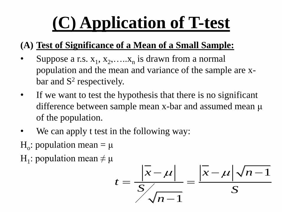
(C) Application of T-test

(A) Test of Significance of a Mean of a Small Sample:

• Suppose a r.s. x1, x2,…..xn is drawn from a normal

population and the mean and variance of the sample are x-

bar and S2 respectively.

• If we want to test the hypothesis that there is no significant

difference between sample mean x-bar and assumed mean μ

of the population.

• We can apply t test in the following way:

Ho: population mean = μ

H1: population mean ≠ μ

1

1

x x nt

S Sn

• The D.f. associated with statistic t is n-1.

• The value of t is compared with the table value

of t on appropriate degree of freedom and at a

required level of significance.

• If tcal < ttab the Ho may be accepted.

• If tcal > ttab the Ho may be rejected.

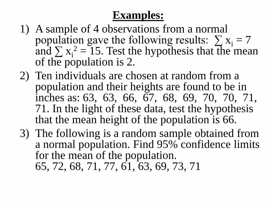
Examples:

1) A sample of 4 observations from a normal population gave the following results: ∑ xi = 7 and ∑ xi

2 = 15. Test the hypothesis that the mean of the population is 2.

2) Ten individuals are chosen at random from a population and their heights are found to be in inches as: 63, 63, 66, 67, 68, 69, 70, 70, 71, 71. In the light of these data, test the hypothesis that the mean height of the population is 66.

3) The following is a random sample obtained from a normal population. Find 95% confidence limits for the mean of the population. 65, 72, 68, 71, 77, 61, 63, 69, 73, 71

(4) For a sample of 9 observations the following

information is obtained. Find 99% C.I. for

population mean.

2

49, (x ) 52.ix x

(B) Test of Significance of difference between

Means of Two Small Samples:

• Suppose two independent small samples of

size n1 and n2 are drawn from two normal

populations and the means of the samples are

x1-bar and x2-bar respectively.

• Under the assumption that both the population

have the same variance.

1 2 1 21 2

1 2

1 2

1 1

x x x x n nt

S n nS

n n

• where

• t is based on n1+n2-2 degrees of freedom.

2 2 2

2 2

1 2

1{ (x ) (x )

2iS x x

n n

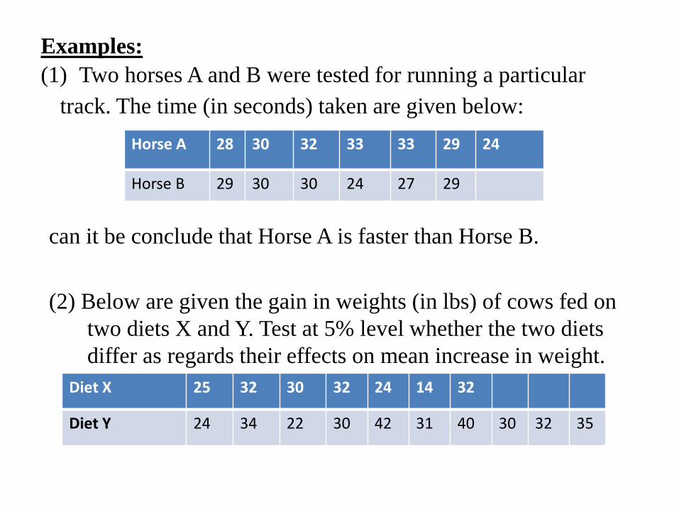
Examples:

(1) Two horses A and B were tested for running a particular

track. The time (in seconds) taken are given below:

can it be conclude that Horse A is faster than Horse B.

(2) Below are given the gain in weights (in lbs) of cows fed on

two diets X and Y. Test at 5% level whether the two diets

differ as regards their effects on mean increase in weight.

Horse A 28 30 32 33 33 29 24

Horse B 29 30 30 24 27 29

Diet X 25 32 30 32 24 14 32

Diet Y 24 34 22 30 42 31 40 30 32 35

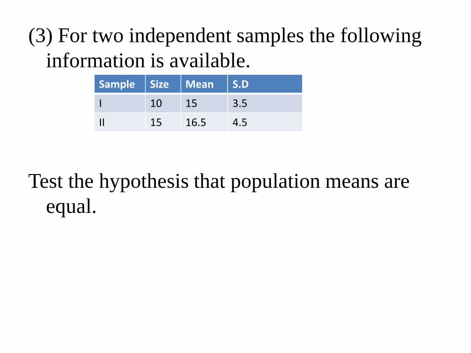
(3) For two independent samples the following

information is available.

Test the hypothesis that population means are

equal.

Sample Size Mean S.D

I 10 15 3.5

II 15 16.5 4.5

Paired t test for difference of means:

• We use the paired t-test when there is one measurement

variable and two nominal variables. One of the nominal

variables has only two values. The most common design is that

one nominal variable represents different individuals, while

the other is "before" and "after" some treatment. Sometimes

the pairs are spatial rather than in order, such as left vs. right,

injured limb vs. uninjured limb, above a dam vs. below a dam,

etc.

• An example would be the performance of undergraduates on a

test of manual dexterity before and after drinking a cup of tea.

For each student, there would be two observations, one before

the tea and one after.

http://udel.edu/~mcdonald/statvartypes.html

http://udel.edu/~mcdonald/statvartypes.html

• Using a paired t-test has much more statistical

power when the difference between groups is

small relative to the variation within groups.

• The paired t-test is only appropriate when

there is just one observation for each

combination of the nominal values. For the tea

example, that would be one measurement of

dexterity on each student before drinking tea,

and one measurement after drinking tea.

Calculation:

• Under the hypothesis that there is no difference in the population, t test can be applied in the following way.

Ho: μ = 0 Vs. H1: μ ≠ 0

• The value of t is computed from the given data and compared with the table value of n-1 degree of freedom.

2 21 1(d )

i

i

dd nt whered andS d

S n n

Examples:

1. The sales data of an item in six shops before and after a special promotion campaign are as under:

Can the campaign be judged as success. Test at 5% L.O.S.

2. A drug is given to 10 patients and the increments in their blood pressure were recorded as

8, 3, 6, 10, 2, -2, 3, 0, -6, 1

Is it reasonable to believe that the drug has no effect on change of B.P.?

shops A B C D E F

Before campaign 53 28 32 48 50 42

After campaign 58 32 30 50 56 45

(D) Large Sample Test: (Z test)

For testing a given hypothesis a random

sample is drawn from a population.

If the number of units in the sample is greater

than 30, it is generally regarded as a large

sample.

Steps for testing a given hypothesis:

1. Starting clearly null and alternative hypothesis.

2. Finding out the difference between observed

value and the value taken in null hypothesis.

3. Calculate S.E. of statistic.

4. Computing the value of Z = difference/ S.E.

The computed value of Z is then compared with the

table value of Z at a rejected level of

significance and the decision regarding

acceptance or rejection of the null hypothesis is

taken.

Critical values at important level of significance

are given below.

1% 5% 10%

Two tailed test 2.58 1.96 1.645

One tailed test 2.33 1.645 1.282

(A)Test of significance of a mean:

Suppose a r.s. of size n is drawn from a large

population.

Suppose the mean of the sample is (x-bar).

If we want to test the hypothesis that

population mean is μ0 i.e.H0 : μ = μ0

(i) H0 : μ = μ0 ; H1 : μ ≠ μ0

(ii) Difference = │(x-bar) - μ0│

(iii) S.E. of (x-bar) = σ / √n

(iv) Z = difference / S.E.

Examples:

1) A sample of 400 students have a mean height of 171.38 cms. Can it be reasonably regarded as a random sample from a large population with mean height 171.17 and standard deviation 3.3 cms.?

2) A stenographer claims that he can write at an average speed of 120 words per minute. In 100 trials he obtained an average speed of 116 words per minute with a S.D. of 15 words. Is the claim justified? Use 5% l.o.s.

3) A random sample of 400 items gave mean 4.5 and variance 4. can the sample be regarded as drawn from a normal population with mean 4?

(B) Test of Significance of difference between two means:

Suppose two independent random samples are drawn from two different populations and their means are respectively x1-bar and x2-bar.

If we want to test the hypothesis that the population means are equal i.e. H0: μ1 = μ2, we can follow the following steps:

(i) H0: μ1 = μ2, H1: μ1 ≠ μ2,

(ii) Difference =

(iii) S.E. of (x1bar - x2bar) =


2 2

1 2

1 2n n

1 2x x

Examples:

(1) The average life of 150 electric bulbs of a company A is 1400 hrs with a S.D. of 120 hrs while the average life of 200 electric bulbs of company B is 1200 hrs. with a S.D. of 80 hrs. Is the difference between the average lives of the bulbs significant?

(2) The mean of a random sample of 1000 units is 17.6 and the mean of another random sample of 800 units is 18. can it be conclude that both the samples come from the same population with S.D. = 2.6.

(3) The average daily wage of 1000 laborers‘ of a factory A is Rs.47 with S.D. of Rs. 28. The average daily wage of 1500 laborers‘ of a factory B is Rs.49 with S.D. of Rs. 40. can it be said that the average daily wage of factory B is more than the average daily wage of factory A?

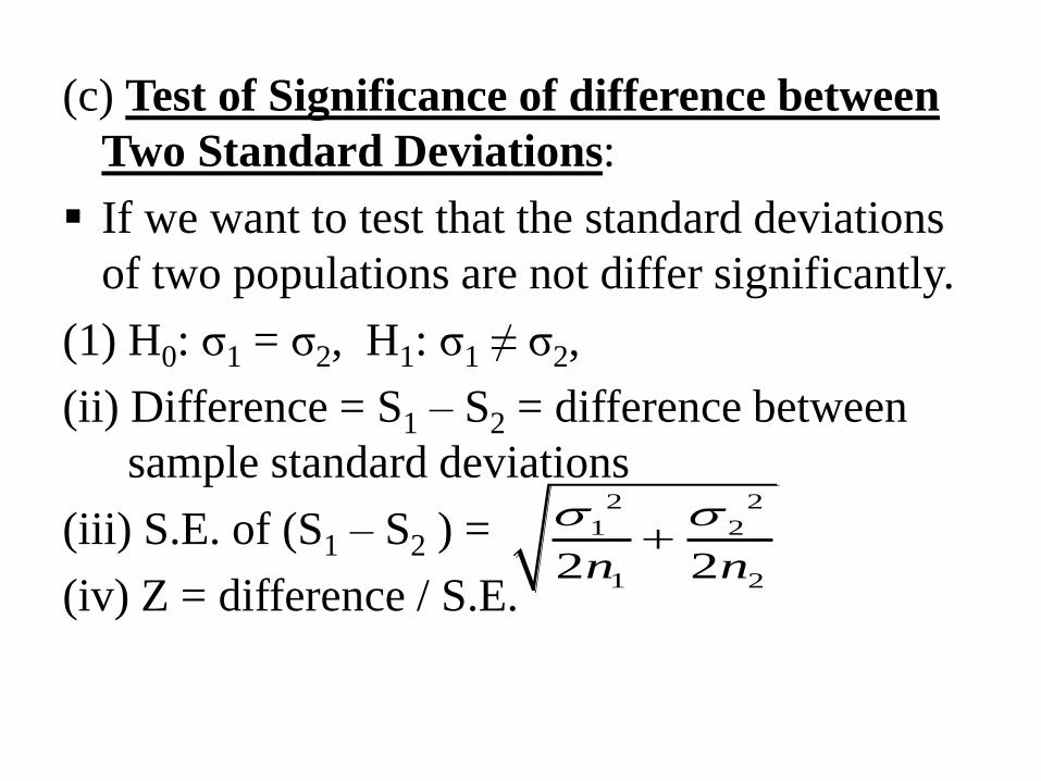
(c) Test of Significance of difference between

Two Standard Deviations:

If we want to test that the standard deviations

of two populations are not differ significantly.

(1) H0: σ1 = σ2, H1: σ1 ≠ σ2,

(ii) Difference = S1 – S2 = difference between

sample standard deviations

(iii) S.E. of (S1 – S2 ) =


2 2

1 2

1 22 2n n

Examples:

(1) The information regarding marks of boys and girls of a

college is given below:

Sample Mean S.D. Sample Size

Boys 83 10 121

Girls 81 12 81

Test whether the difference in standard deviation is significant.

(2)From the following data, test whether the difference between standard deviations is significant or not?

S.D. Size

Sample-I 53.83 1390

Sample-II 56.56 630

Education

Unit 3