Phenomenology of large scale structure

Ravi K Sheth (ICTP/UPenn)

• The Halo Model–Observations/Motivation

• The Excursion Set approach–The ansatz–Correlated steps–Large scale bias–Ensemble averages: Halos and peaks–Modified gravity

Galaxy spatial distribution depends on galaxy type (luminosity, color, etc.)

Not all galaxies can be unbiased tracers of the underlying Mass distribution

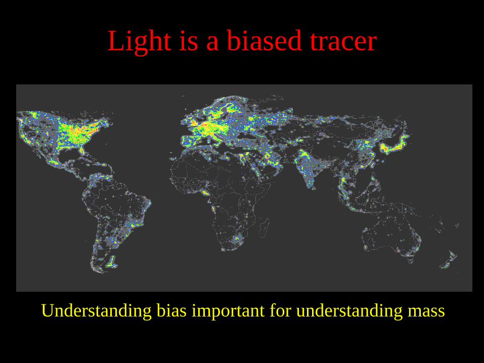
Light is a biased tracer

Understanding bias important for understanding mass

How to describe different point processes which are all built from the same underlying distribution?

THE HALO MODEL

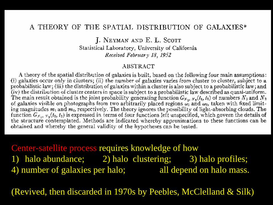
Center-satellite process requires knowledge of how 1) halo abundance; 2) halo clustering; 3) halo profiles; 4) number of galaxies per halo; all depend on halo mass.

(Revived, then discarded in 1970s by Peebles, McClelland & Silk)

The halo-model of clustering• Two types of pairs: both particles in same halo, or

particles in different halos

• ξobs(r) = ξ1h(r) + ξ2h(r)

• All physics can be decomposed similarly: ‘nonlinear’ effects from within halo, ‘linear’ from outside

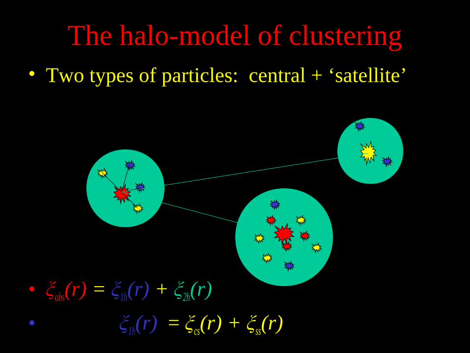
The halo-model of clustering• Two types of particles: central + ‘satellite’

• ξobs(r) = ξ1h(r) + ξ2h(r)

• ξ1h(r) = ξcs(r) + ξss(r)

To implement Neyman-Scott program

need model for cluster abundance

and cluster clustering

Next generation of surveys will have 109 galaxies in105 clusters

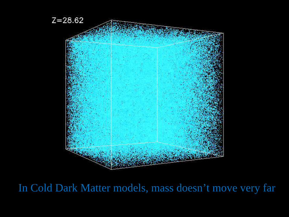
In Cold Dark Matter models, mass doesn’t move very far

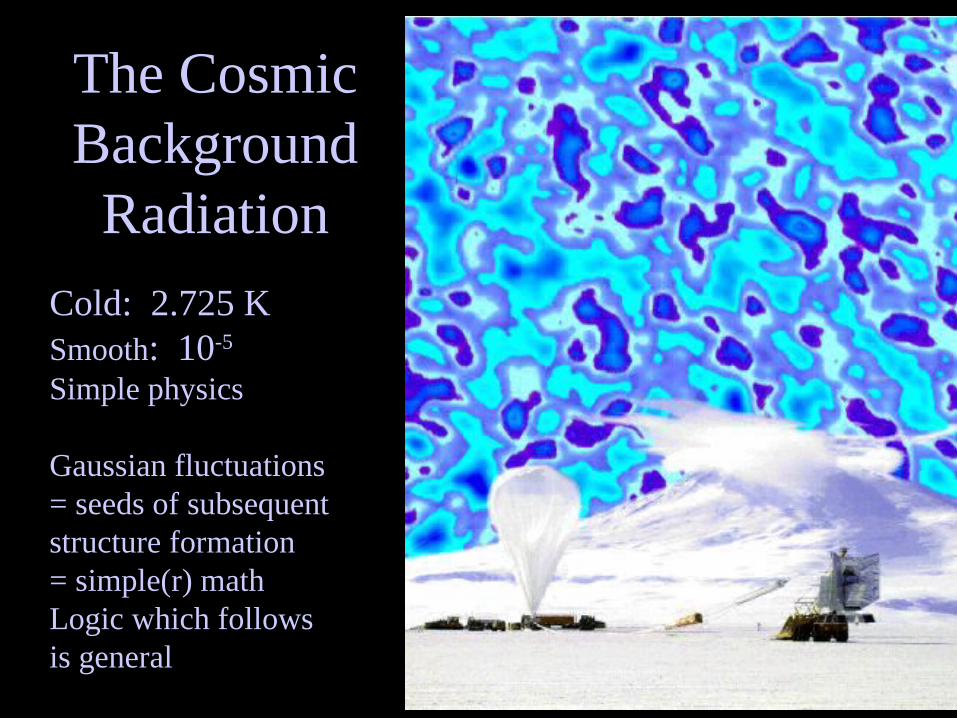
The Cosmic Background

Radiation

Cold: 2.725 KSmooth: 10-5

Simple physics

Gaussian fluctuations = seeds of subsequent structure formation = simple(r) mathLogic which follows is general

Birkhoff’s theorem important

Use initial conditions (CMB) +

model of nonlinear gravitational clustering

to make inferences about late-time, nonlinear structures

Hierarchical clustering in GR

= the persistence of memory

THE EXCURSION SET APPROACH

(Epstein 1983; Bond et al. 1991; Lacey & Cole 1993; Sheth 1998; Sheth & van de Weygaert 2004; Shen et al. 2006)

N-body simulations of

gravitational clustering

in an expanding universe

Assume a spherical cow …

(Gunn & Gott 1972)

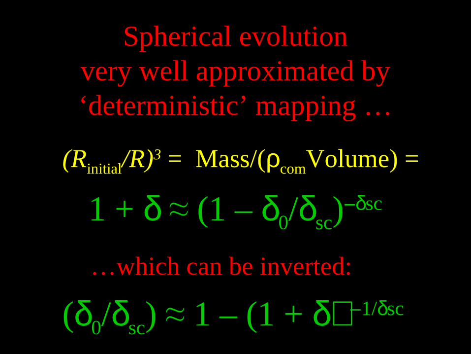
Spherical evolutionvery well approximated by ‘deterministic’ mapping …

(Rinitial/R)3 = Mass/(ρcomVolume) =

1 + δ ≈ (1 – δ0/δsc)−δsc

…which can be inverted:

(δ0/δsc) ≈ 1 – (1 + δ) 1/− δsc

δcrit

δ0(M/V)

Linear theory over-density

MASS

Halo of mass m<M within this patch (M,v)

This patch of volume v contains mass M

The Nonlinear PDF

V v

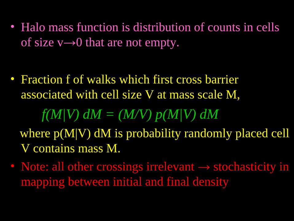
• Halo mass function is distribution of counts in cells of size v→0 that are not empty.

• Fraction f of walks which first cross barrier associated with cell size V at mass scale M,

f(M|V) dM = (M/V) p(M|V) dM where p(M|V) dM is probability randomly placed cell

V contains mass M.

• Note: all other crossings irrelevant → stochasticity in mapping between initial and final density

Higher RedshiftCritical

over-density

MASS

smaller mass patch within more massive region

This patch forms halo of mass M

The Random Walk Model

From Walks to Halos: Ansätze

• f(δc,s)ds = fraction of walks which first cross δc(z) at s

≈ fraction of initial volume in patches of comoving volume V(s) which were just dense enough to collapse at z

≈ fraction of initial mass in regions which each initially contained m =ρV(1+δc) ≈ ρV(s) and which were just dense enough to collapse at z (ρ is comoving density of background)

≈ dm m n(m,δc)/ρ

High-z

Low-zover-density

MASS

small mass at high-z

larger mass at low z

Random Walk = Accretion history

Major merger

‘sm

ooth

’

accr

etion

Time evolution of barrier depends on cosmology

Mapping between σ2 and M depends on P(k)

σ2(M)

Simplification because…

• Everything local• Evolution determined by cosmology (competition

between gravity and expansion)• Statistics determined by initial fluctuation field:

since Gaussian, statistics specified by initial power-spectrum P(k)

• Fact that only very fat cows are spherical is a detail (crucial for precision cosmology); in excursion set approach, mass-dependent barrier height increases with distance along walk

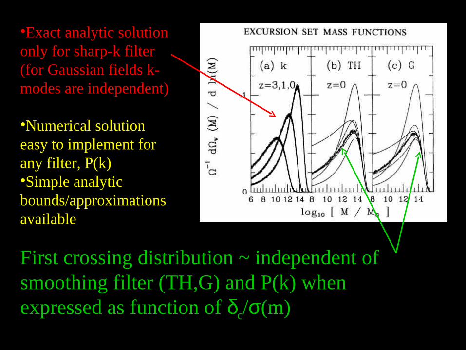
First crossing distribution ~ independent of smoothing filter (TH,G) and P(k) when expressed as function of δc/σ(m)

•Exact analytic solution only for sharp-k filter (for Gaussian fields k-modes are independent)

•Numerical solution easy to implement for any filter, P(k)•Simple analytic bounds/approximations available

Assumptions of convenience• Uncorrelated steps

– Correlated steps (Peacock & Heavens 1990; Bond et al. 1991;

Maggiore & Riotto 2010; Paranjape et al. 2011)

– Non-Gaussian mass function (Matarrese et al. 2001) ~ given by changing PDF but keeping uncorrelated steps (Lam & Sheth 2009)

• Barrier is sharp – Fuzzy/porous barriers (Sheth, Mo, Tormen 2001; Sheth

&Tormen 2002 ; Maggiore & Riotto 2010; Paranjape et al 2011)

• Ensemble of walks is also random – The real cloud-in-cloud problem

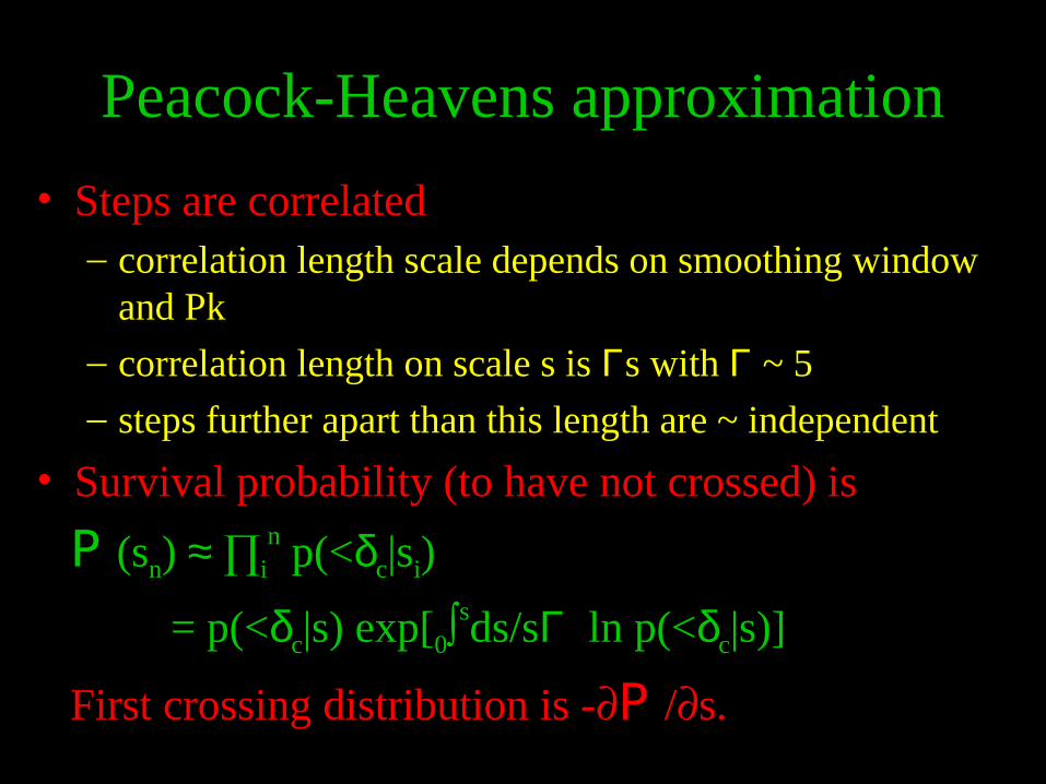
Peacock-Heavens approximation

• Steps are correlated– correlation length scale depends on smoothing window

and Pk– correlation length on scale s is Γs with Γ ~ 5– steps further apart than this length are ~ independent

• Survival probability (to have not crossed) is

P (sn) ≈ ∏in p(<δc|si)

= p(<δc|s) exp[0∫sds/sΓ ln p(<δc|s)]

First crossing distribution is -∂P / s.∂

Critical

over-density

MASS

Typical mass smaller at early times: hierarchical clustering

Completely correlated steps

Critical

initialover-density

MASS

Easier to get here from over-dense environment

This patch forms halo of mass M

Correlations with environment

over-dense

under-dense

‘Top-heavy’ mass function in dense regions

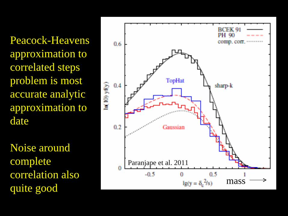
Paranjape et al. 2011

Peacock-Heavens approximation to correlated steps problem is most accurate analytic approximation to date

Noise around complete correlation also quite good

mass

Extensions (Paranjape, Lam, Sheth 2011)

– conditional distributions (environmental trends)– large-scale bias – can both be understood as arising from fact that

p(x|y) = Gaussian with <x|y> = y <xy>/<yy>– so simply make this replacement in PH expressions– moving barriers (ellipsoidal collapse, PDF),

• Generalization of PH to constrained walks:

p(<δc|s) p(<→ δc,s|δ0, S0)

is trivial and accurate

δ1 – (Sx/S0) δ0

ν10 = ------------------ √S1- (Sx/S0)2 S0

• Read fine print (and correct the typos!) in Bond et al. (1991)

mass

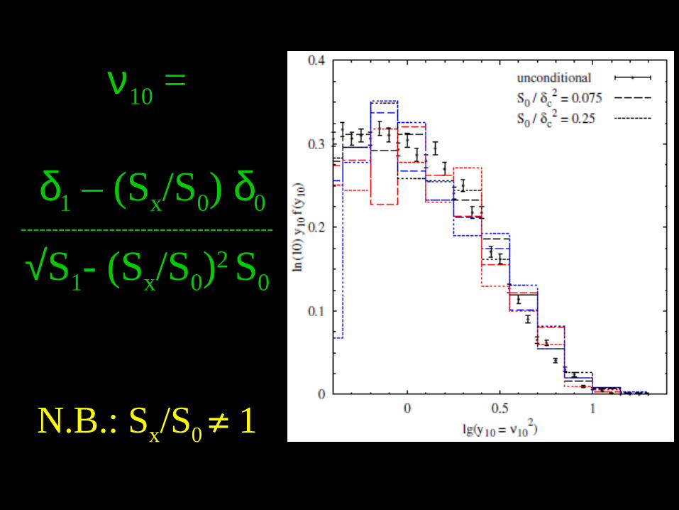
ν10 =

δ1 – (Sx/S0) δ0----------------------------------------

√S1- (Sx/S0)2 S0

N.B.: Sx/S0 1≠

Large scale bias

• f(m|δ0)/f(m) – 1 ~ f(ν10)/f(ν) – 1

~ (Sx/S) b(ν) δ0

where b is usual (Mo-White) bias factor

• So, real space bias should differ from Fourier space bias by factor (Sx/S)

• N.B. exactly same effect seen for peaks (Desjacques et al. 2010); in essence, this is same calculation as the ‘peak’ density profile (BBKS 1986)

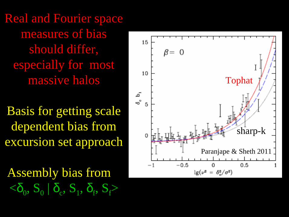
Real and Fourier space measures of bias

should differ, especially for most

massive halos

Basis for getting scale dependent bias from

excursion set approach

Assembly bias from <δ0, S0 | δc, S1, δf, Sf>

Paranjape & Sheth 2011

Tophat

sharp-k

Most of apparent difference is due to difference between real and Fourier space bias

Real difference in Fourier space bias is small – but significant at small masses

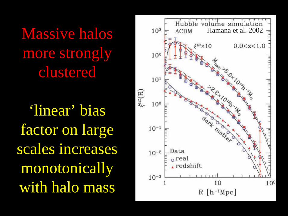
Massive halos more strongly

clustered

‘linear’ bias factor on large scales increases monotonically with halo mass

Hamana et al. 2002

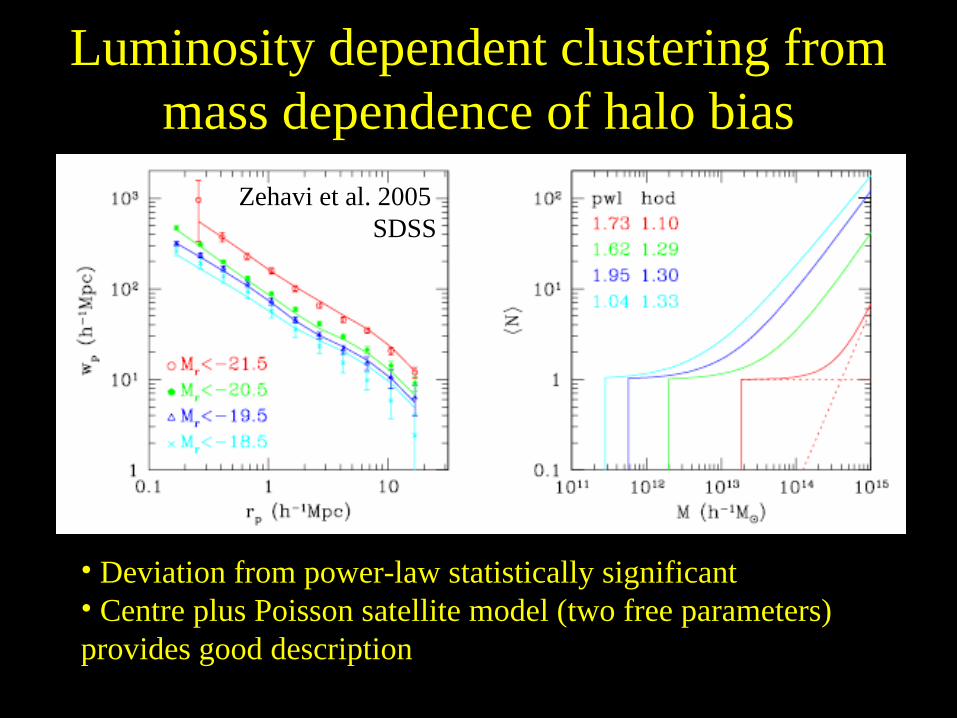
Luminosity dependent clustering from mass dependence of halo bias

Zehavi et al. 2005 SDSS

• Deviation from power-law statistically significant• Centre plus Poisson satellite model (two free parameters) provides good description

Summary• Intimate connection between abundance and

clustering of dark halos– Can use cluster clustering as check that cluster mass-

observable relation correctly calibrated– Almost all correlations with environment arise through halo

bias (massive halos populate densest regions)

• Next step in random walk ~ independent of previous – History of object ~ independent of environment– Not true for correlated steps

• Description quite detailed; sufficiently accurate to complete Neyman-Scott program (The Halo Model)

Success to date motivates search for more accurate

(better than 10%) models of halo

abundance/clustering:

Quest for Halo Grail?

Work in progress• Correlated steps

– Assembly bias

• Correlated walks – What is correct ensemble?

– Generically increase high-m abundance (ST99 parameter ‘a’)

• Dependence on parameters other than δ – Higher dimensional walks

– What is correct basis set? (e,p)? (I2,I3)?

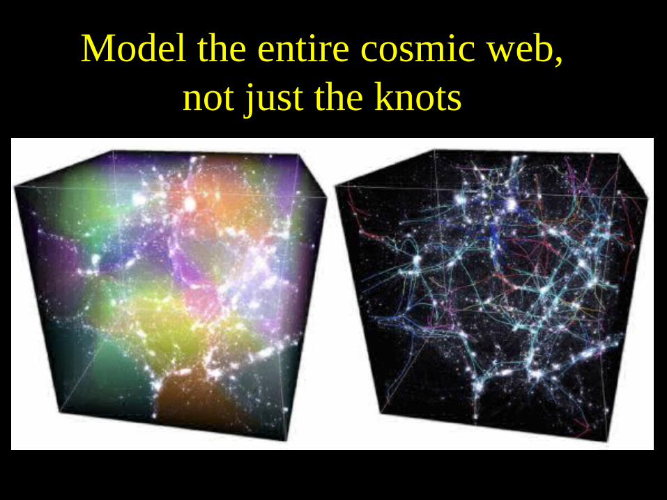
Model the entire cosmic web, not just the knots

Study of random walks with correlated steps

(i.e. path integral methods) =

Cosmological constraints from large scale structures

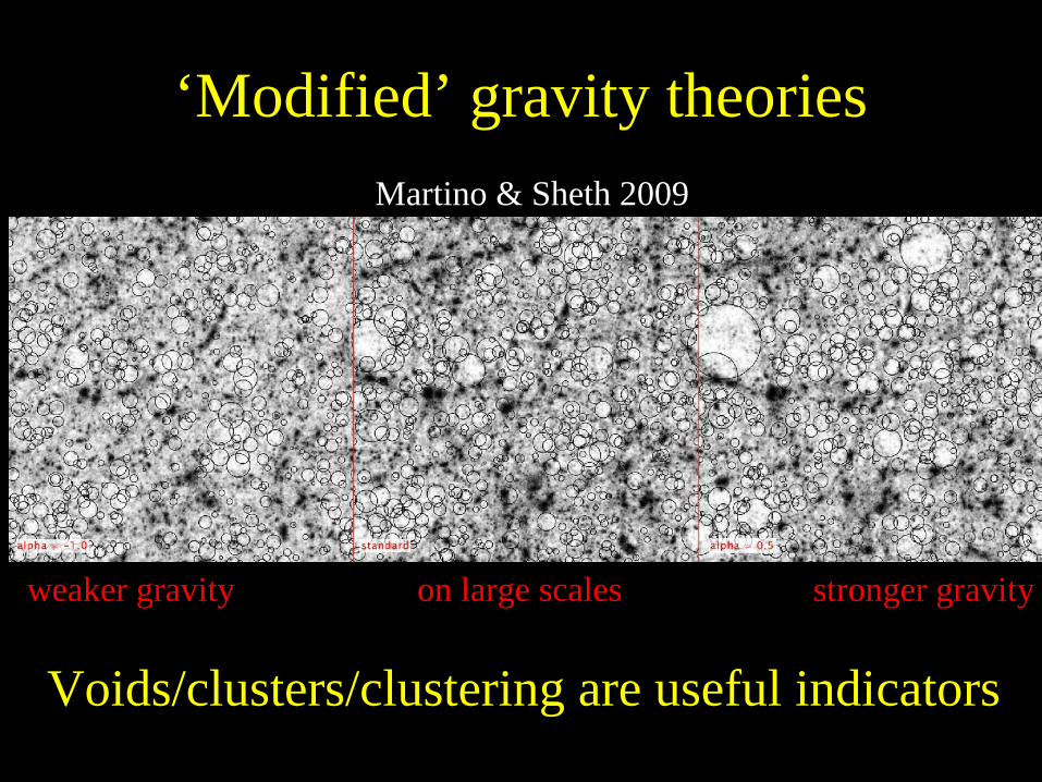
‘Modified’ gravity theories

Voids/clusters/clustering are useful indicators

weaker gravity on large scales stronger gravity

Martino & Sheth 2009

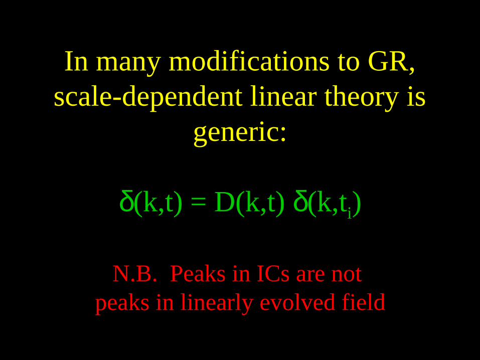
In many modifications to GR,scale-dependent linear theory is

generic:

δ(k,t) = D(k,t) δ(k,ti)

N.B. Peaks in ICs are not peaks in linearly evolved field

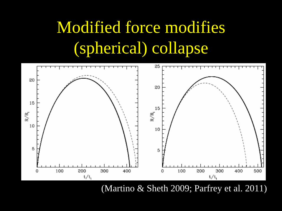
Modified force modifies (spherical) collapse

(Martino & Sheth 2009; Parfrey et al. 2011)

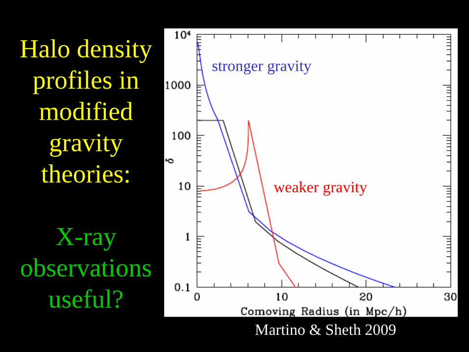
Halo density profiles in modified gravity

theories:

X-ray observations

useful?

stronger gravity

weaker gravity

Martino & Sheth 2009

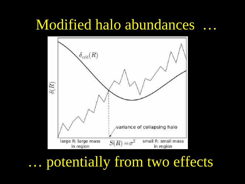
Modified halo abundances …

… potentially from two effects

δc(m) and σ(m)

• In standard GR, σ(m) is an integral over initial P(k), evolved using linear theory to later (collapse) time.

• In modified theories, D(k,t) means there is a difference between calculating in ICs vs linearly evolved field.

• Energy conservation arguments suggest better to work in ICs.

Critical overdensity required for

collapse at present becomes mass

dependent: δc(m)

This is generic.

Implication for halo bias

• Halos are linearly biased tracers of initial field

• D(k) means they are not linearly biased tracers of linearly-evolved field (Parfrey et al. 2011)

• Simulations in hand too small to test, but if real, this is an important systematic