CENTURION UNIVERSITY OF TECHNOLOGY & MANAGEMENT

A L L U R I N A G A R , P A R A L A K H E M U N D I .

2014

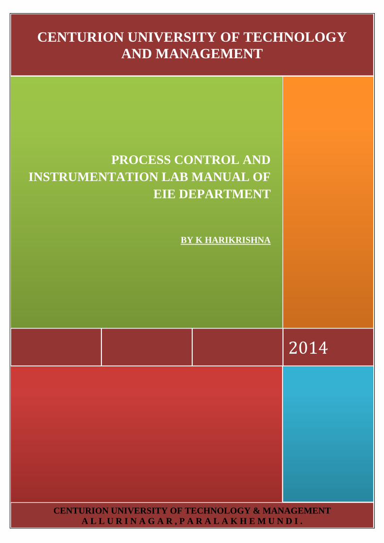
PROCESS CONTROL AND

INSTRUMENTATION LAB MANUAL OF

EIE DEPARTMENT

BY K HARIKRISHNA

CENTURION UNIVERSITY OF TECHNOLOGY

AND MANAGEMENT

1

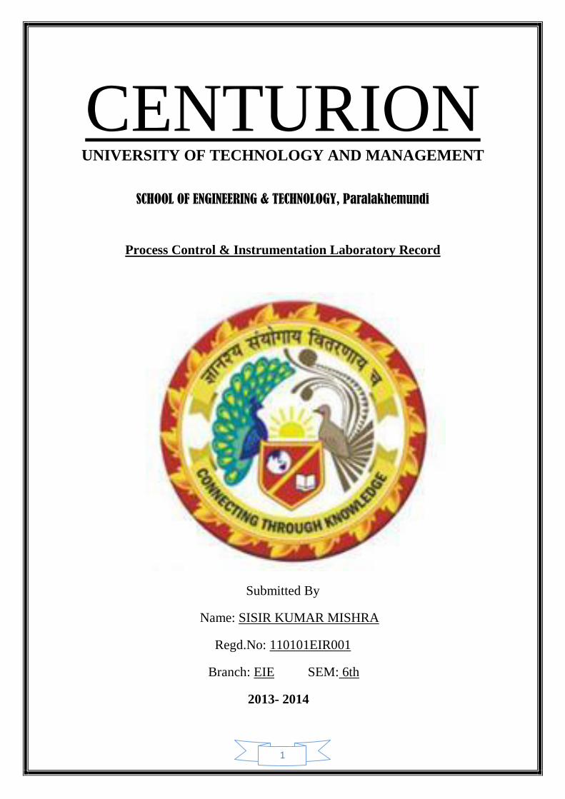
CENTURION UNIVERSITY OF TECHNOLOGY AND MANAGEMENT

SCHOOL OF ENGINEERING & TECHNOLOGY, Paralakhemundi

Process Control & Instrumentation Laboratory Record

Submitted By

Name: SISIR KUMAR MISHRA

Regd.No: 110101EIR001

Branch: EIE SEM: 6th

2013- 2014

2

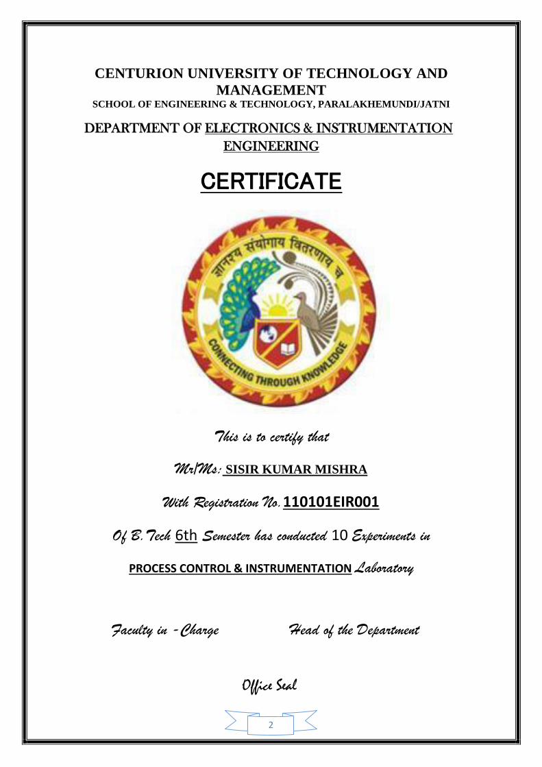
CENTURION UNIVERSITY OF TECHNOLOGY AND

MANAGEMENT SCHOOL OF ENGINEERING & TECHNOLOGY, PARALAKHEMUNDI/JATNI

DEPARTMENT OF ELECTRONICS & INSTRUMENTATION

ENGINEERING

CERTIFICATE

This is to certify that

Mr/Ms: SISIR KUMAR MISHRA

With Registration No.110101EIR001

Of B.Tech 6th Semester has conducted 10 Experiments in

PROCESS CONTROL & INSTRUMENTATION Laboratory

Faculty in -Charge Head of the Department

Office Seal

3

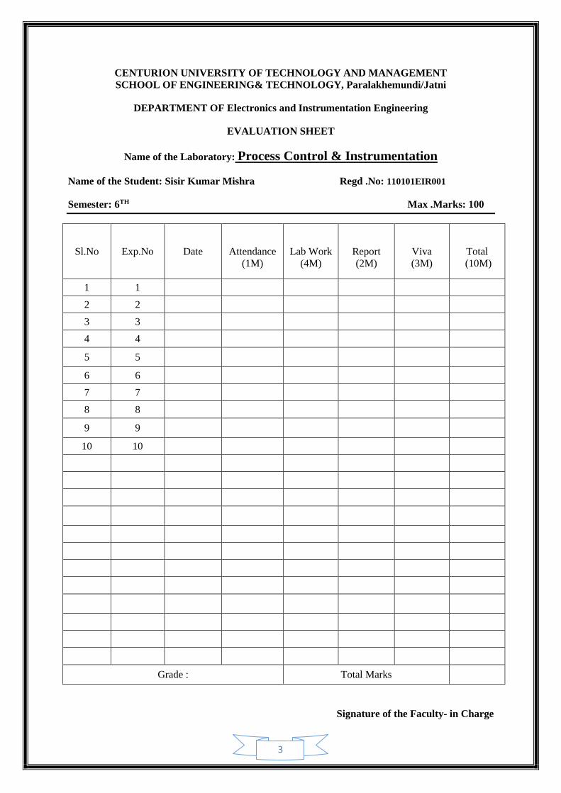
CENTURION UNIVERSITY OF TECHNOLOGY AND MANAGEMENT

SCHOOL OF ENGINEERING& TECHNOLOGY, Paralakhemundi/Jatni

DEPARTMENT OF Electronics and Instrumentation Engineering

EVALUATION SHEET

Name of the Laboratory: Process Control & Instrumentation

Name of the Student: Sisir Kumar Mishra Regd .No: 110101EIR001

Semester: 6TH Max .Marks: 100

Sl.No Exp.No Date

Attendance

(1M)

Lab Work

(4M)

Report

(2M)

Viva

(3M)

Total

(10M)

1 1

2 2

3 3

4 4

5 5

6 6

7 7

8 8

9 9

10 10

Grade : Total Marks

Signature of the Faculty- in Charge

4

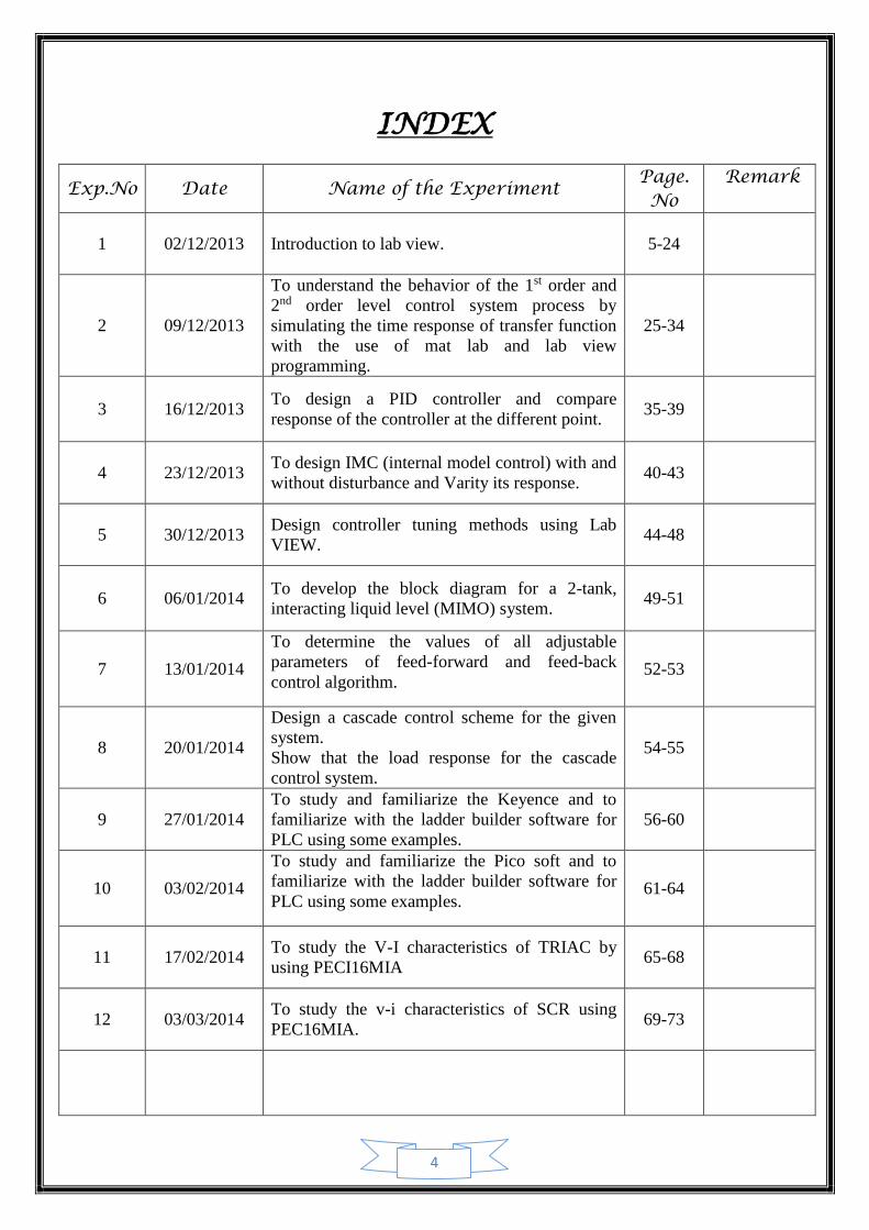
INDEX

Exp.No Date Name of the Experiment Page. No

Remark

1 02/12/2013 Introduction to lab view. 5-24

2 09/12/2013

To understand the behavior of the 1st order and

2nd order level control system process by

simulating the time response of transfer function

with the use of mat lab and lab view

programming.

25-34

3 16/12/2013 To design a PID controller and compare

response of the controller at the different point. 35-39

4 23/12/2013 To design IMC (internal model control) with and

without disturbance and Varity its response. 40-43

5 30/12/2013 Design controller tuning methods using Lab

VIEW. 44-48

6 06/01/2014 To develop the block diagram for a 2-tank,

interacting liquid level (MIMO) system. 49-51

7 13/01/2014

To determine the values of all adjustable

parameters of feed-forward and feed-back

control algorithm. 52-53

8 20/01/2014

Design a cascade control scheme for the given

system.

Show that the load response for the cascade

control system.

54-55

9 27/01/2014

To study and familiarize the Keyence and to

familiarize with the ladder builder software for

PLC using some examples.

56-60

10 03/02/2014

To study and familiarize the Pico soft and to

familiarize with the ladder builder software for

PLC using some examples. 61-64

11 17/02/2014 To study the V-I characteristics of TRIAC by

using PECI16MIA 65-68

12 03/03/2014 To study the v-i characteristics of SCR using

PEC16MIA. 69-73

5

EXPERIMENT-1

AIM OF THE EXPERIMENT:-

Introduction to lab view

SOFTWARE REQUIRED:-

Lab view 2010

THEORY:-

Introduction Lab VIEW:

Lab VIEW is a development system for industrial, experimental, and educational

measurement and automation applications based on graphical programming, in contrast to

textual programming - however, textual programming is supported in Lab VIEW.

Lab VIEW has a large number of functions for numerical analysis and design and

visualization of data.

Lab VIEW now has several toolkits and modules which brings the Lab VIEW to the same

level of functionality as Matlab and Simulink in analysis and design in the areas of control,

signal processing, system identification, mathematics, and simulation, and more.

In addition, Lab VIEW has, of course, inbuilt support for the broad range of measurement

and automation hardware produced by National Instruments. Communication with third party

hardware is also possible thanks to the availability of a large number of drivers and the

support for communication standards as OPC, Modbus, GPIB, etc.

Lab VIEW is produced by National Instruments.

Lab VIEW (short for Laboratory Virtual Instrumentation Engineering Workbench) is a

platform and development environment for a visual programming language from National

Instruments. The purpose of such programming is automating the usage of processing and

measuring equipment in any laboratory setup.

The graphical language is named "G" (not to be confused with G-code). Originally released

for the Apple Macintosh in 1986, Lab VIEW is commonly used for data acquisition,

instrument control, and industrial automation on a variety of platforms including Microsoft

Windows, various versions of UNIX, Linux, and Mac OS X.

The programming language used in Lab VIEW, also referred to as G, is a dataflow

programming language.

Execution is determined by the structure of a graphical block diagram (the LV-source code)

on which the programmer connects different function-nodes by drawing wires.

These wires propagate variables and any node can execute as soon as all its input data

become available. Since this might be the case for multiple nodes simultaneously, G is

inherently capable of parallel execution. Multi-processing and multi-threading hardware is

6

automatically exploited by the built-in scheduler, which multiplexes multiple OS threads over

the nodes ready for execution.

Lab VIEW ties the creation of user interfaces (called front panels) into the development

cycle. Lab VIEW programs/subroutines are called virtual instruments (VIs).

Each VI has three components: a block diagram, a front panel and a connector panel.

The last is used to represent the VI in the block diagrams of other, calling VIs. Controls and

indicators on the front panel allow an operator to input data into or extract data from a

running virtual instrument.

However, the front panel can also serve as a programmatic interface.

Thus a virtual instrument can either be run as a program, with the front panel serving as a

user interface, or, when dropped as a node onto the block diagram, the front panel defines the

inputs and outputs for the given node through the connector pane.

The graphical approach also allows non-programmers to build programs by dragging and

dropping virtual representations of lab equipment with which they are already familiar. The

Lab VIEW programming environment, with the included examples and documentation,

makes it simple to create small applications. This is a benefit on one side, but there is also a

certain danger of underestimating the expertise needed for high-quality G programming

. For complex algorithms or large-scale code, it is important that the programmer possesses

an extensive knowledge of the special Lab VIEW syntax and the topology of its memory

management. The most advanced Lab VIEW development systems offer the possibility of

building stand-alone applications. Furthermore, it is possible to create distributed

applications, which communicate by a client/server scheme, and are therefore easier to

implement due to the inherently parallel nature of G.

Command lab view short cut:

File:

Clrtl+N = create new VI

Clrtl+O = open file

Clrtl+W = close file

Clrtl+S = save VI

Clrtl+I = display VI properties

Clrtl+Q = quit Lab VIEW

Edit:

Clrtl+V = paste object

Clrtl+Shift+F = display search results

Clrtl+U = clean up diagram

Clrtl+space = activate quick drop

Clrtl+B = remove broken wires 3

Clrtl+X = cut object

Clrtl+Z = undo last action

Clrtl+Shift+z = redo last action

7

Operate:

Clrtl+R = run VI

Clrtl+M = change run /edit node

Clrtl = atomic VI

Window:

Clrtl+E = display block diagram / front panel

Right click =display controls/functions palette

Shift = display tool palette

Clrtl+L = display error list

Clrtl+T = title block diagram and front panel windows

Clrtl+l = adjust window to full size

Help:

Clrtl+H = display window to full size

Clrtl+? = display help contents & index

Clrtl+Shift +L = lock context help

National instruments of lab view is an industry leading software tool for designing test,

National Instruments Lab VIEW is an industry-leading software tool for designing test,

measurement, and control systems.

Since its introduction in 1986, engineers and scientists worldwide who have relied on NI Lab

VIEW graphical development for projects throughout the product design cycle have gained

improved quality, shorter time to market, and greater engineering and manufacturing

efficiency.

By using the integrated Lab VIEW environment to interface with real-world signals, analyze

data for meaningful information, and share results, you can boost productivity throughout

your organization.

Because Lab VIEW has the flexibility of a programming language combined with built-in

tools designed specifically for test, measurement, and control, you can create applications

that range from simple temperature monitoring to sophisticated simulation and control

systems.

No matter what your project is, Lab VIEW has the necessary tools to make you successful

quickly.

.

This course prepares you to do the following:

• Use LabVIEW to create applications.

8

• Understand front panels, block diagrams, and icons and connector panes.

• Use built-in LabVIEW functions.

• Create and save programs in LabVIEW so you can use them as subroutines.

• Create applications that use plug-in DAQ devices.

This course does not describe any of the following:

• Programming theory

• Every built-in LabVIEW function or object

• Analog-to-digital (A/D) theory

NI does provide free reference materials on the above topics on ni.com.

Virtual Instrumentation:-

For more than 30 years, National Instruments has revolutionized the way engineers and

scientists in industry, government, and academia approach measurement and automation.

Leveraging PCs and commercial technologies, virtual instrumentation increases productivity

and lowers costs for test, control, and design applications through easy-to-integrate software,

such as NI Lab VIEW, and modular measurement and control hardware for PXI, PCI, USB,

and Ethernet.

With virtual instrumentation, engineers use graphical programming software to create user-

defined solutions that meet their specific needs, which is a great alternative to proprietary,

fixed-functionality traditional instruments.

Additionally, virtual instrumentation capitalizes on the ever-increasing performance of

personal computers.

For example, in test, measurement, and control, engineers have used virtual instrumentation

to downsize automated test equipment (ATE) while experiencing up to a 10 times increase in

productivity gains at a fraction of the cost of traditional instrument solutions.

Virtual Instrumentation Applications:-

Virtual instrumentation is effective in many different types of applications, from design to

prototyping to deployment.

The Lab VIEW platform provides specific tools and models to meet specific application

challenges, ranging from designing signal processing algorithms to making voltage

measurements, and can target any number of platforms from the desktop to embedded

devices – with an intuitive, powerful graphical paradigm. Lab VIEW scales from design and

development on PCs to several embedded targets, from rugged toaster-size prototypes to

embedded systems on chips.

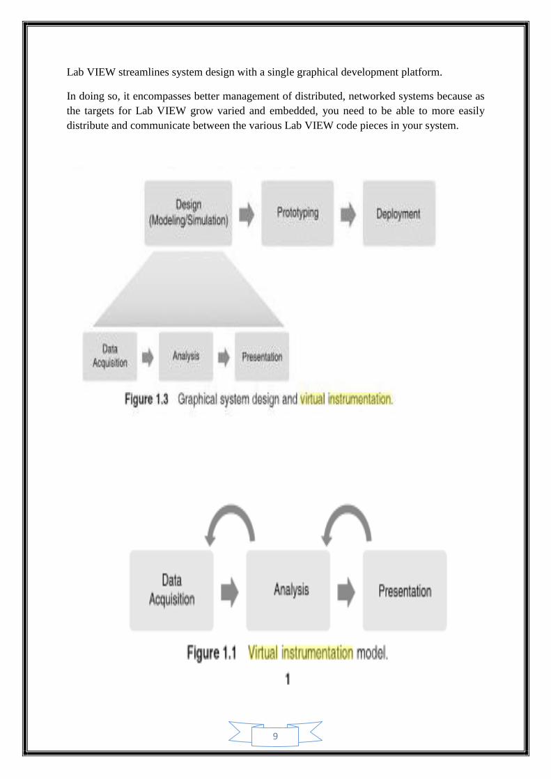
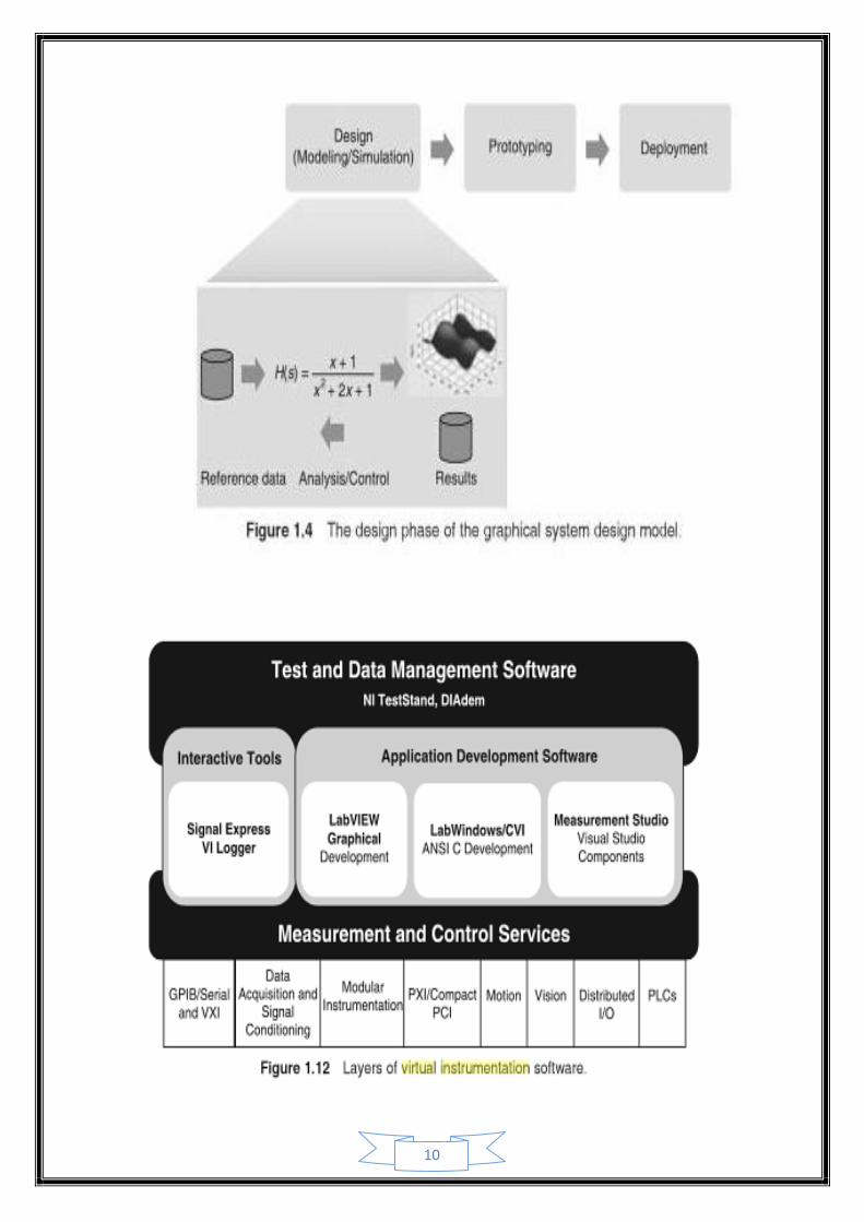
9

Lab VIEW streamlines system design with a single graphical development platform.

In doing so, it encompasses better management of distributed, networked systems because as

the targets for Lab VIEW grow varied and embedded, you need to be able to more easily

distribute and communicate between the various Lab VIEW code pieces in your system.

10

11

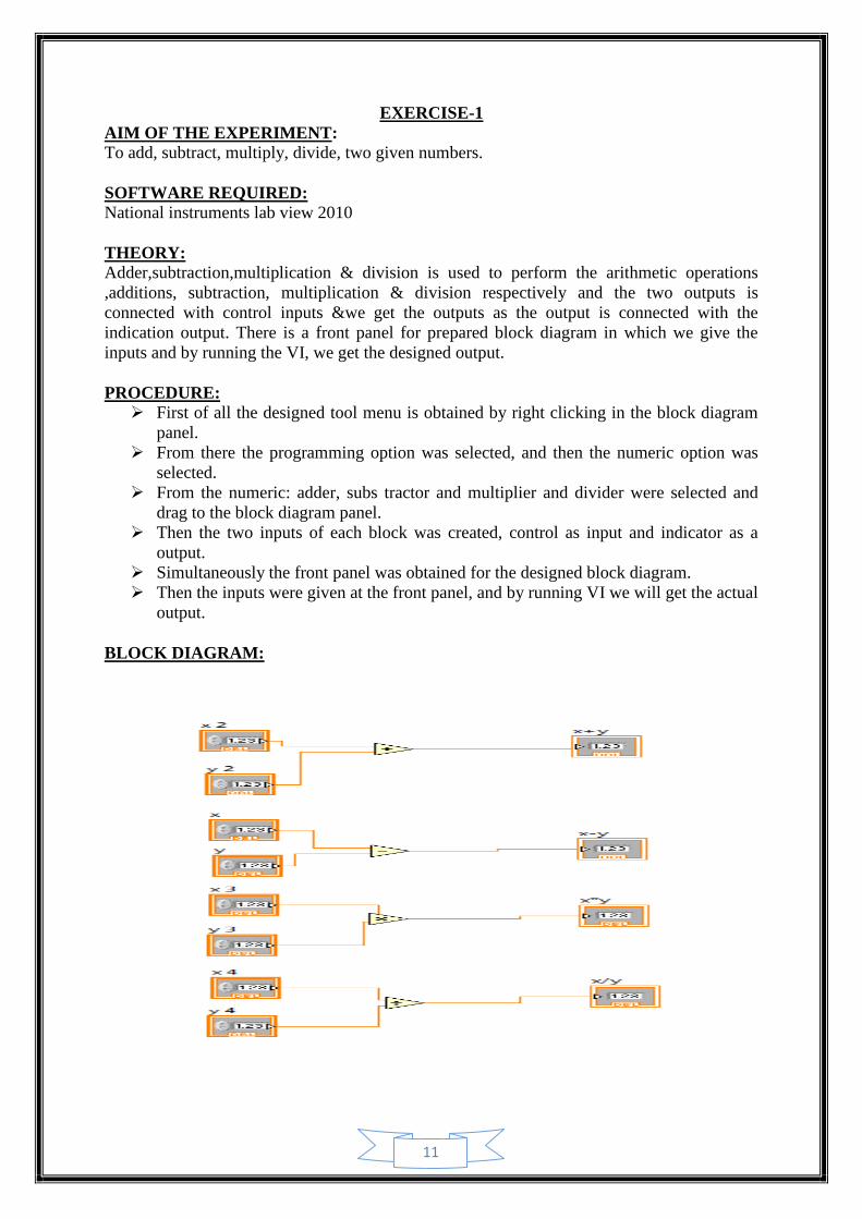
EXERCISE-1

AIM OF THE EXPERIMENT: To add, subtract, multiply, divide, two given numbers.

SOFTWARE REQUIRED: National instruments lab view 2010

THEORY:

Adder,subtraction,multiplication & division is used to perform the arithmetic operations

,additions, subtraction, multiplication & division respectively and the two outputs is

connected with control inputs &we get the outputs as the output is connected with the

indication output. There is a front panel for prepared block diagram in which we give the

inputs and by running the VI, we get the designed output.

PROCEDURE: First of all the designed tool menu is obtained by right clicking in the block diagram

panel.

From there the programming option was selected, and then the numeric option was

selected.

From the numeric: adder, subs tractor and multiplier and divider were selected and

drag to the block diagram panel.

Then the two inputs of each block was created, control as input and indicator as a

output.

Simultaneously the front panel was obtained for the designed block diagram.

Then the inputs were given at the front panel, and by running VI we will get the actual

output.

BLOCK DIAGRAM:

12

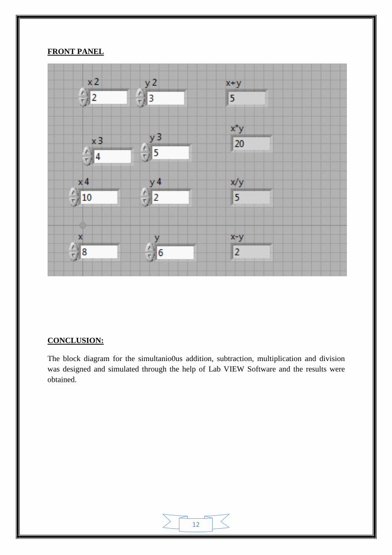
FRONT PANEL

CONCLUSION:

The block diagram for the simultanio0us addition, subtraction, multiplication and division

was designed and simulated through the help of Lab VIEW Software and the results were

obtained.

13

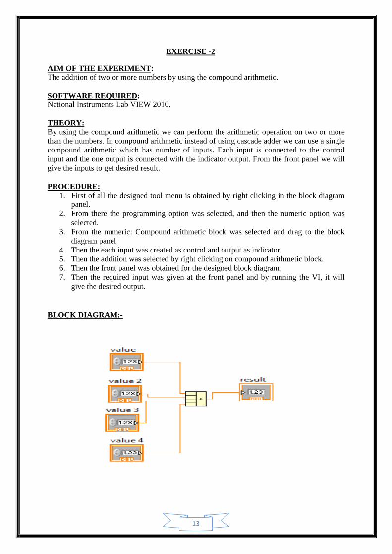
EXERCISE -2

AIM OF THE EXPERIMENT: The addition of two or more numbers by using the compound arithmetic.

SOFTWARE REQUIRED: National Instruments Lab VIEW 2010.

THEORY: By using the compound arithmetic we can perform the arithmetic operation on two or more

than the numbers. In compound arithmetic instead of using cascade adder we can use a single

compound arithmetic which has number of inputs. Each input is connected to the control

input and the one output is connected with the indicator output. From the front panel we will

give the inputs to get desired result.

PROCEDURE:

1. First of all the designed tool menu is obtained by right clicking in the block diagram

panel.

2. From there the programming option was selected, and then the numeric option was

selected.

3. From the numeric: Compound arithmetic block was selected and drag to the block

diagram panel

4. Then the each input was created as control and output as indicator.

5. Then the addition was selected by right clicking on compound arithmetic block.

6. Then the front panel was obtained for the designed block diagram.

7. Then the required input was given at the front panel and by running the VI, it will

give the desired output.

BLOCK DIAGRAM:-

14

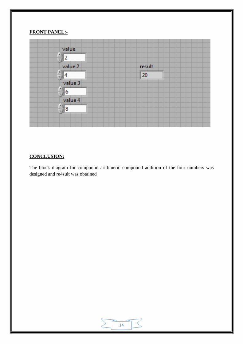
FRONT PANEL:-

CONCLUSION:

The block diagram for compound arithmetic compound addition of the four numbers was

designed and re4sult was obtained

15

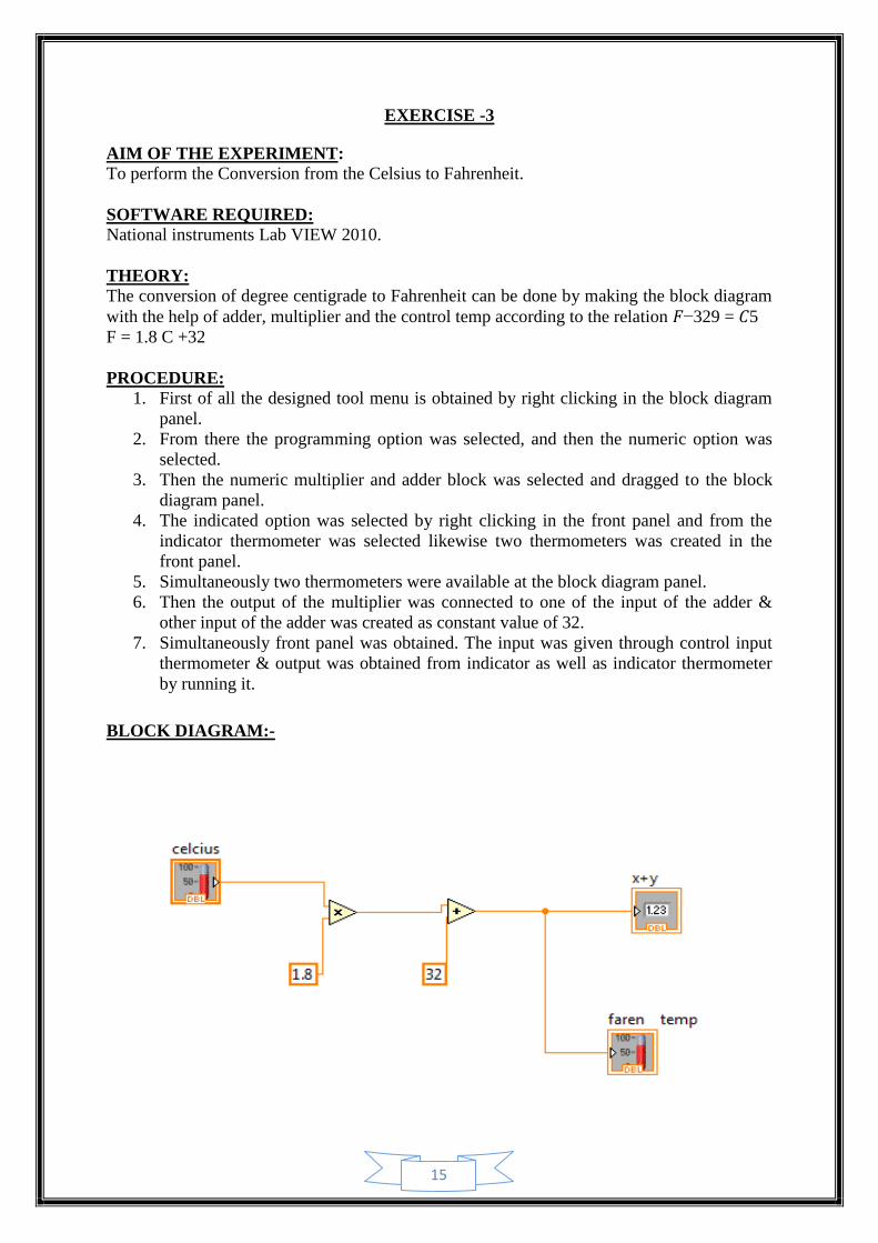
EXERCISE -3

AIM OF THE EXPERIMENT:

To perform the Conversion from the Celsius to Fahrenheit.

SOFTWARE REQUIRED: National instruments Lab VIEW 2010.

THEORY:

The conversion of degree centigrade to Fahrenheit can be done by making the block diagram

with the help of adder, multiplier and the control temp according to the relation 𝐹−329 = 𝐶5

F = 1.8 C +32

PROCEDURE: 1. First of all the designed tool menu is obtained by right clicking in the block diagram

panel.

2. From there the programming option was selected, and then the numeric option was

selected.

3. Then the numeric multiplier and adder block was selected and dragged to the block

diagram panel.

4. The indicated option was selected by right clicking in the front panel and from the

indicator thermometer was selected likewise two thermometers was created in the

front panel.

5. Simultaneously two thermometers were available at the block diagram panel.

6. Then the output of the multiplier was connected to one of the input of the adder &

other input of the adder was created as constant value of 32.

7. Simultaneously front panel was obtained. The input was given through control input

thermometer & output was obtained from indicator as well as indicator thermometer

by running it.

BLOCK DIAGRAM:-

16

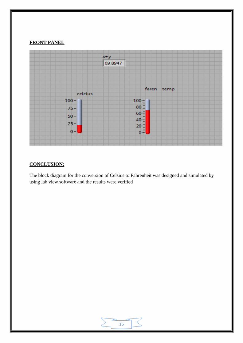
FRONT PANEL

CONCLUSION:

The block diagram for the conversion of Celsius to Fahrenheit was designed and simulated by

using lab view software and the results were verified

17

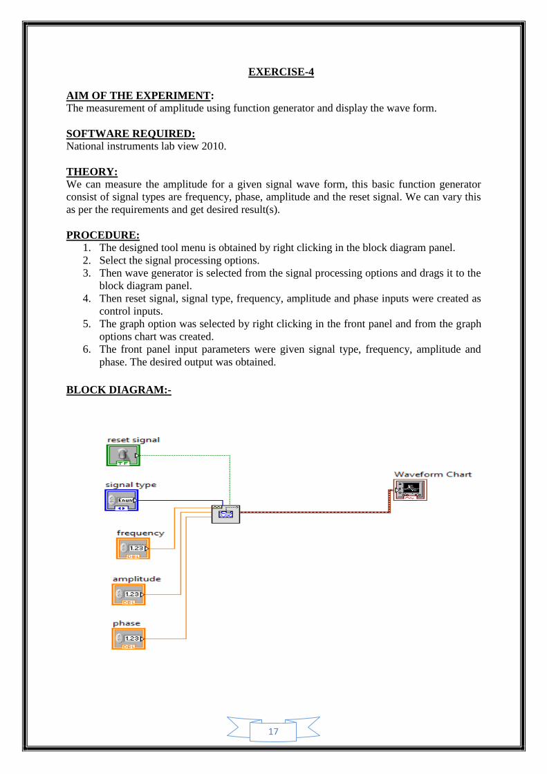
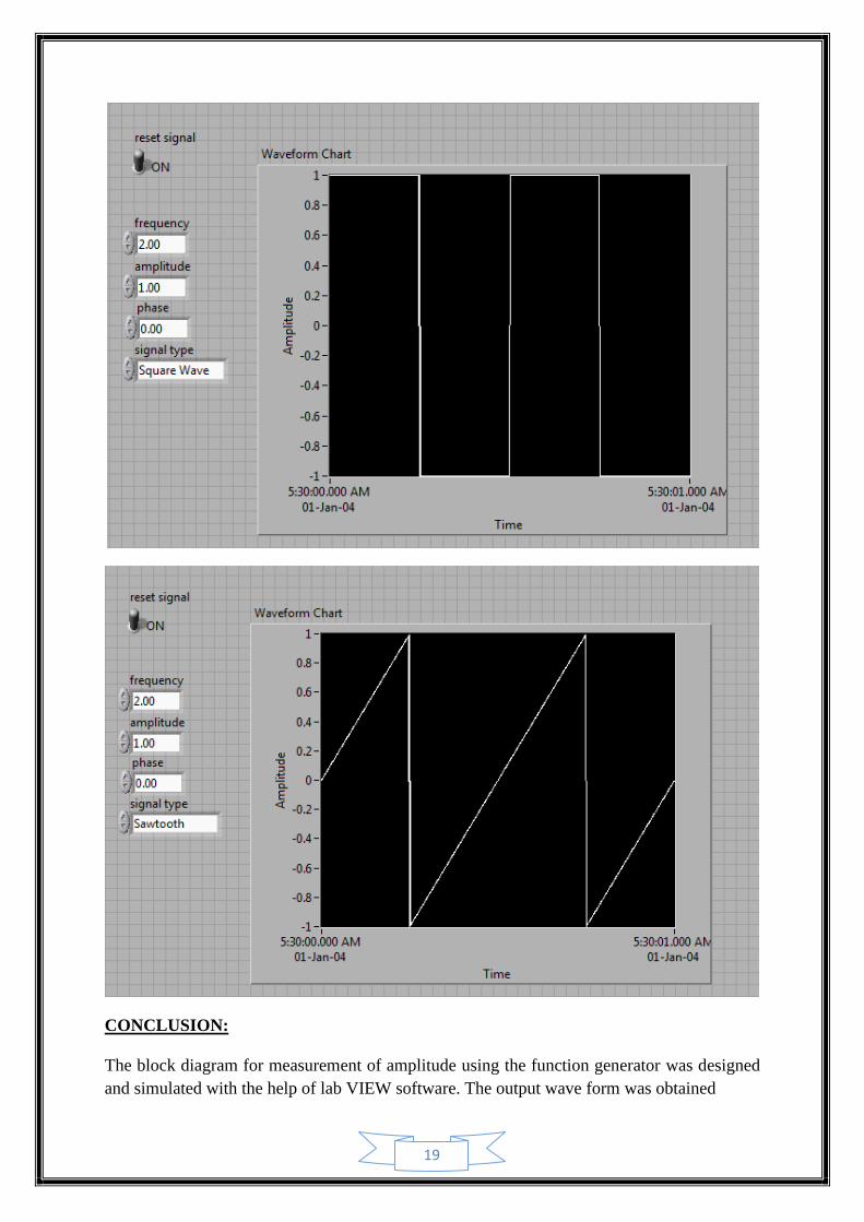
EXERCISE-4

AIM OF THE EXPERIMENT: The measurement of amplitude using function generator and display the wave form.

SOFTWARE REQUIRED: National instruments lab view 2010.

THEORY: We can measure the amplitude for a given signal wave form, this basic function generator

consist of signal types are frequency, phase, amplitude and the reset signal. We can vary this

as per the requirements and get desired result(s).

PROCEDURE: 1. The designed tool menu is obtained by right clicking in the block diagram panel.

2. Select the signal processing options.

3. Then wave generator is selected from the signal processing options and drags it to the

block diagram panel.

4. Then reset signal, signal type, frequency, amplitude and phase inputs were created as

control inputs.

5. The graph option was selected by right clicking in the front panel and from the graph

options chart was created.

6. The front panel input parameters were given signal type, frequency, amplitude and

phase. The desired output was obtained.

BLOCK DIAGRAM:-

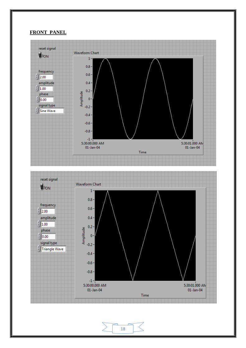
18

FRONT PANEL

19

CONCLUSION:

The block diagram for measurement of amplitude using the function generator was designed

and simulated with the help of lab VIEW software. The output wave form was obtained

20

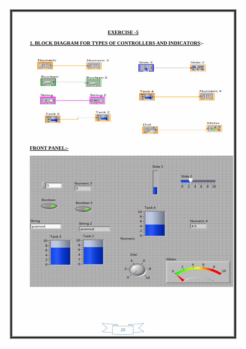
EXERCISE -5

1. BLOCK DIAGRAM FOR TYPES OF CONTROLLERS AND INDICATORS:-

FRONT PANEL:-

21

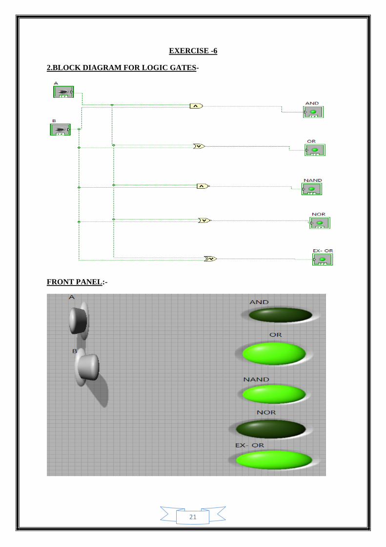
EXERCISE -6

2.BLOCK DIAGRAM FOR LOGIC GATES-

FRONT PANEL:-

22

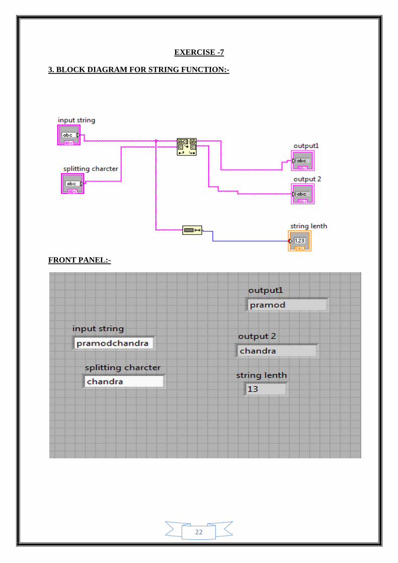
EXERCISE -7

3. BLOCK DIAGRAM FOR STRING FUNCTION:-

FRONT PANEL:-

23

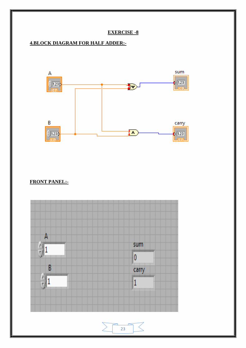
EXERCISE -8

4.BLOCK DIAGRAM FOR HALF ADDER:-

FRONT PANEL:-

24

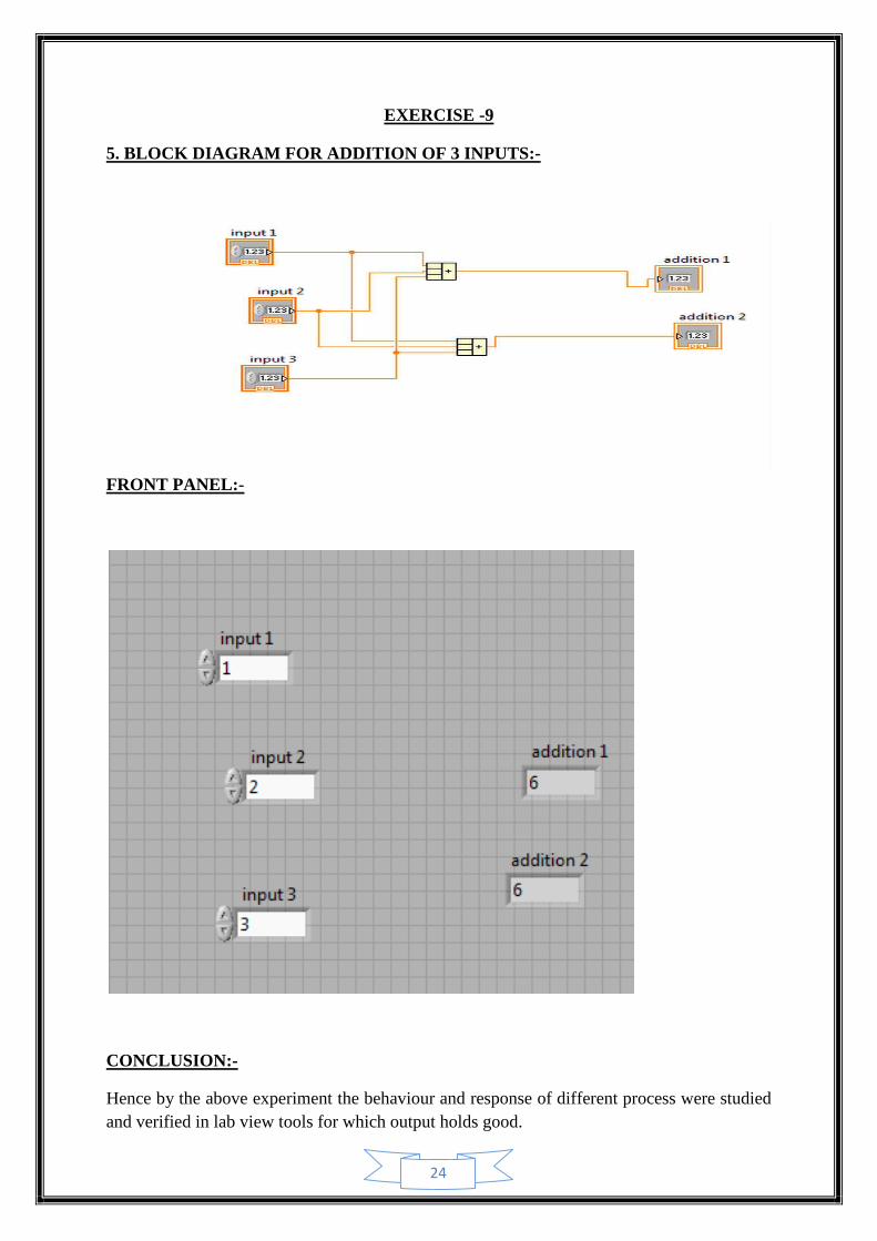
EXERCISE -9

5. BLOCK DIAGRAM FOR ADDITION OF 3 INPUTS:-

FRONT PANEL:-

CONCLUSION:-

Hence by the above experiment the behaviour and response of different process were studied

and verified in lab view tools for which output holds good.

25

EXPERIMENT-2

AIM OF THE EXPERIMENT

To understand the behaviour of the 1st order and 2nd order level control system process by

simulating the time response of transfer function with the use of mat lab and lab view

programming.

SOFTWARE REQUIRED

1. Mat lab R2010a

2. Lab view 2009

THEORY

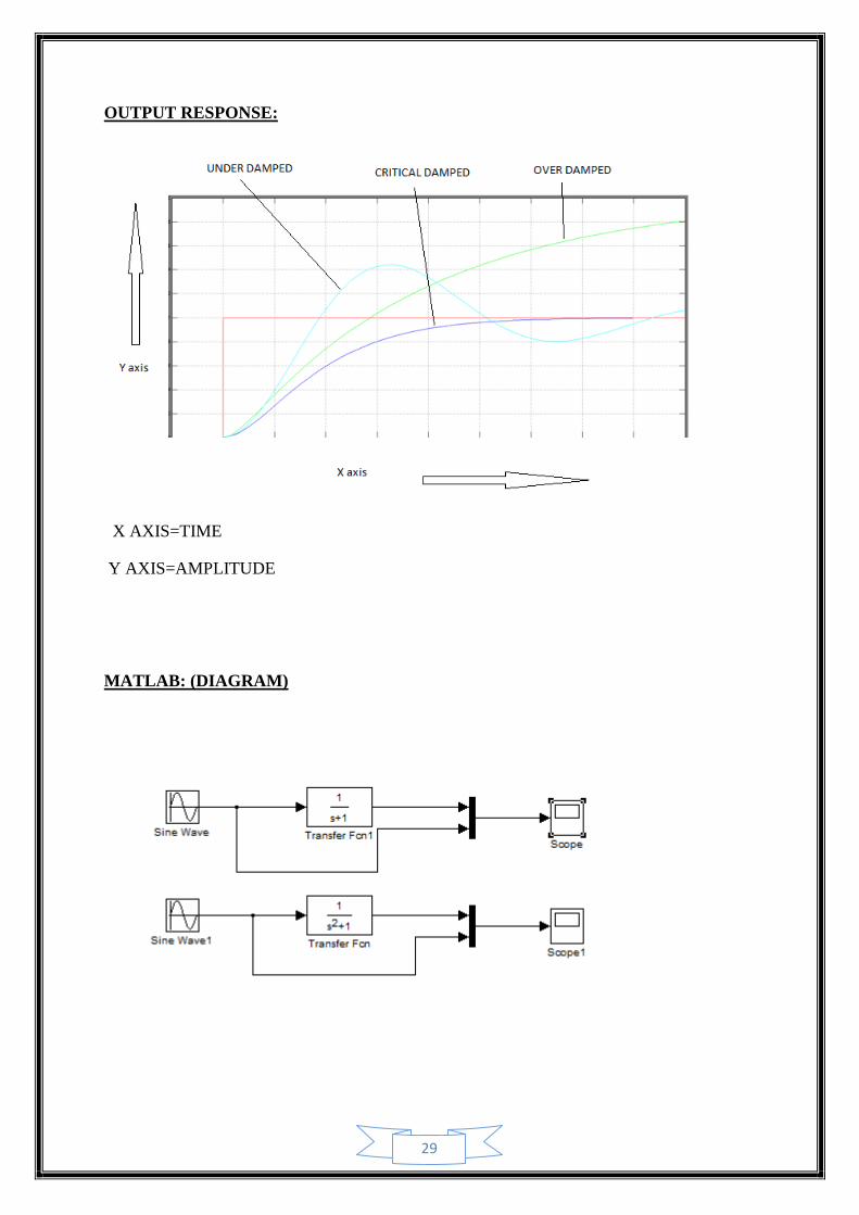
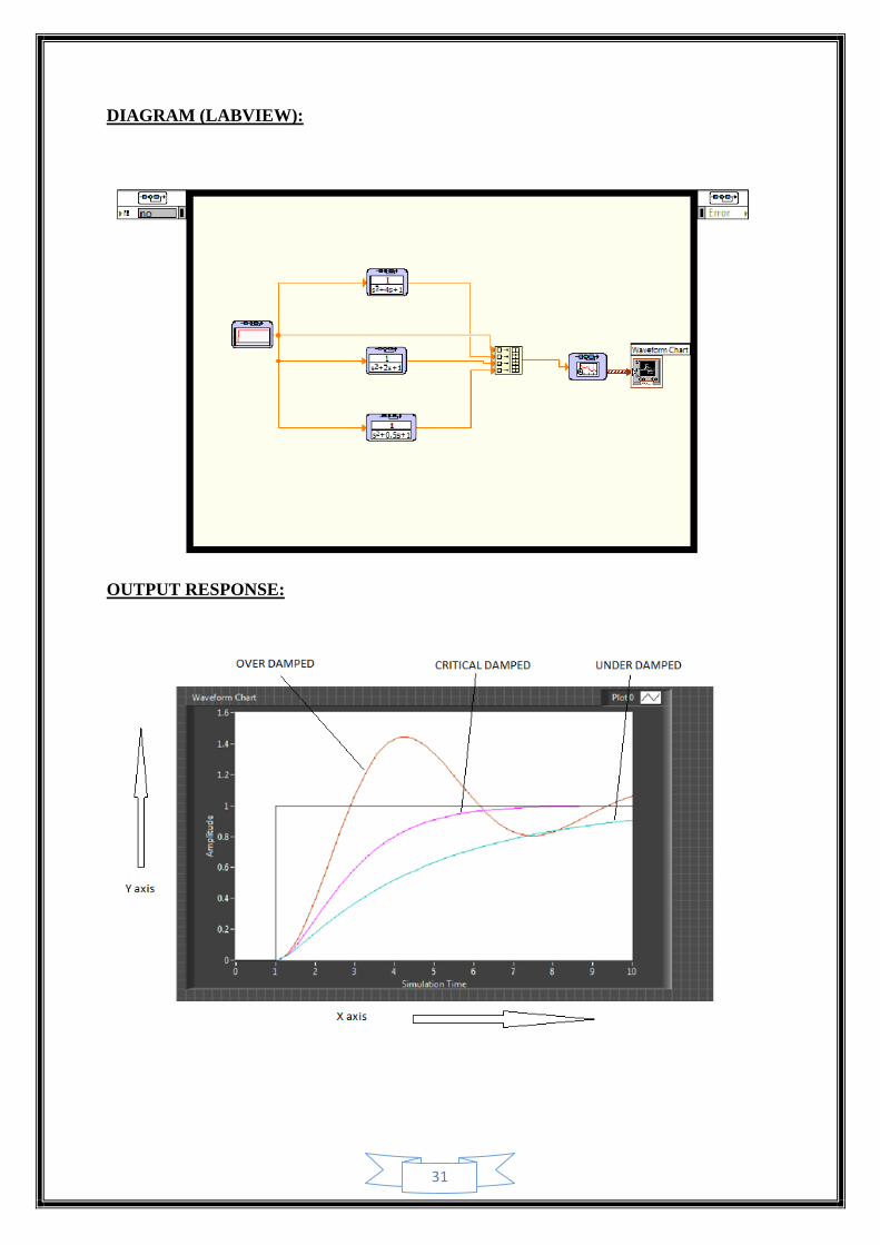
Every practical system takes finite time to reach its steady state and during this period, it

oscillates or increases exponentially .every system has a tendency to oppose oscillatory

behaviour of the system which is called damping. This damping is measured by a factor or a

ratio called damping ratio of the system. A standard second order system takes the transfer

function.

𝐶(𝑠)

𝑅(𝑠) =

𝜔𝑛²

𝑠2+2𝜉𝜔𝑛𝑠+𝜔𝑛²

For 1˂ ξ ˂∞

The output is purely exponentially .this means damping is so high that there are no oscillation

in the output and is purely exponential. Hence such system are called over damped

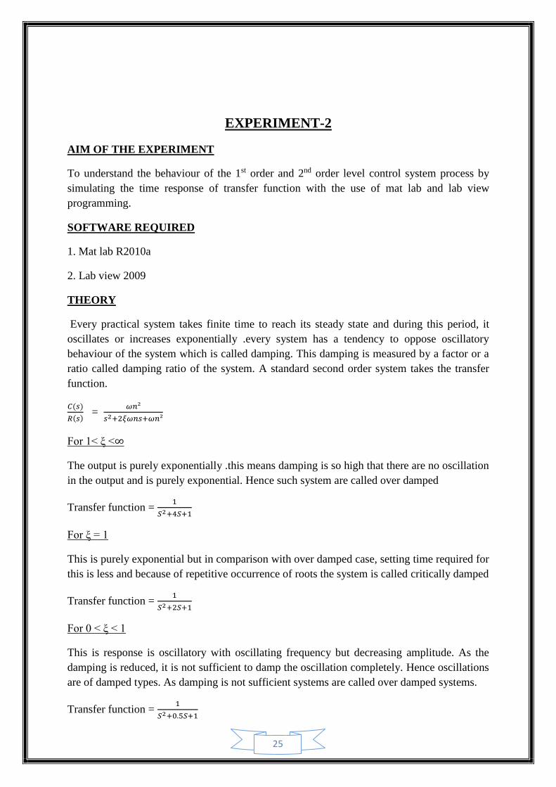
Transfer function = 1

𝑆2+4𝑆+1

For ξ = 1

This is purely exponential but in comparison with over damped case, setting time required for

this is less and because of repetitive occurrence of roots the system is called critically damped

Transfer function = 1

𝑆2+2𝑆+1

For 0 ˂ ξ ˂ 1

This is response is oscillatory with oscillating frequency but decreasing amplitude. As the

damping is reduced, it is not sufficient to damp the oscillation completely. Hence oscillations

are of damped types. As damping is not sufficient systems are called over damped systems.

Transfer function = 1

𝑆2+0.5𝑆+1

26

DIAGRAM: (MATLAB)

OUTPUT RESPONSE:

X AXIS=TIME

Y AXIS=AMPLITUDE

27

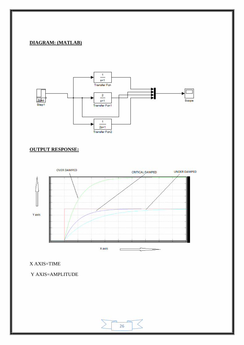
DIAGRAM: (MATLAB)

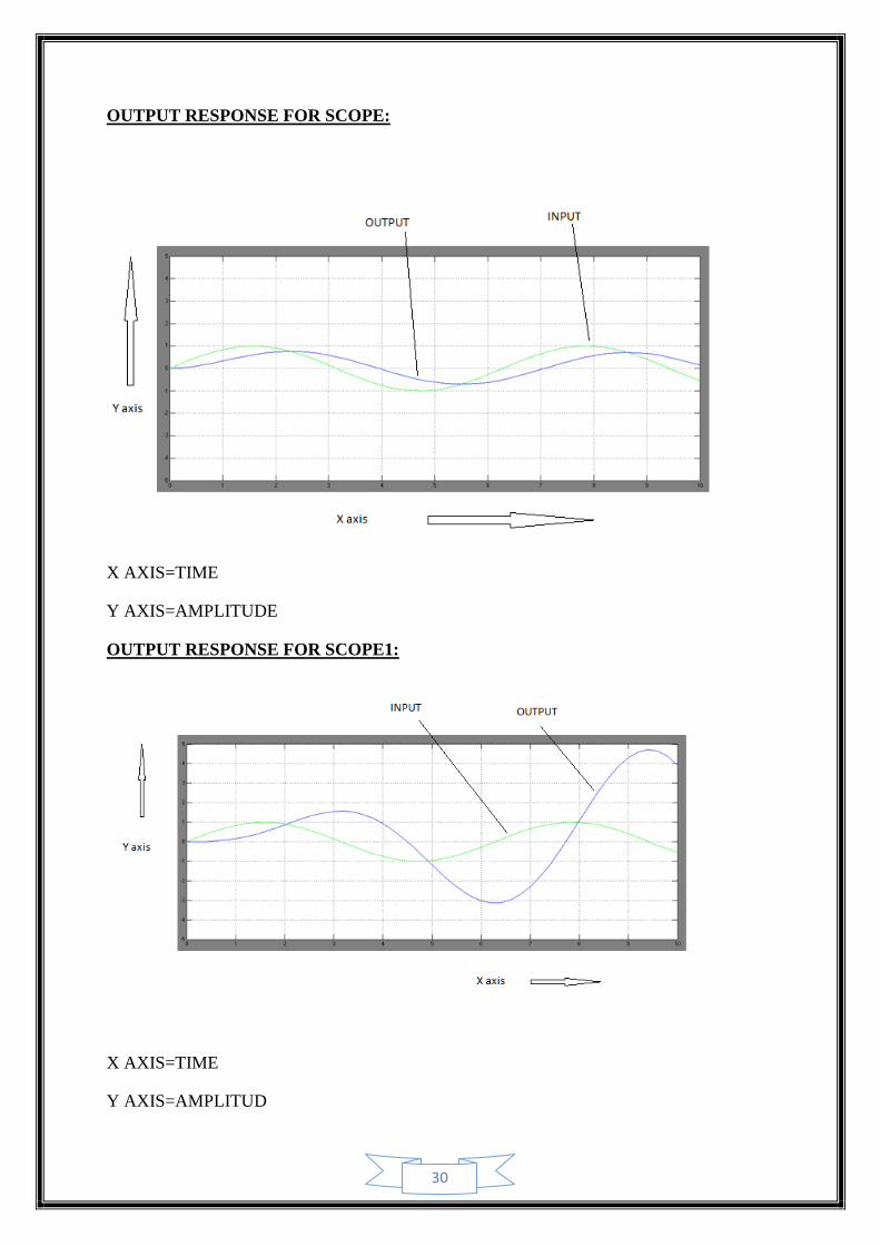
OUTPUT RESPONSE FOR SCOPE:

X AXIS=TIME

Y AXIS=AMPLITUDE

28

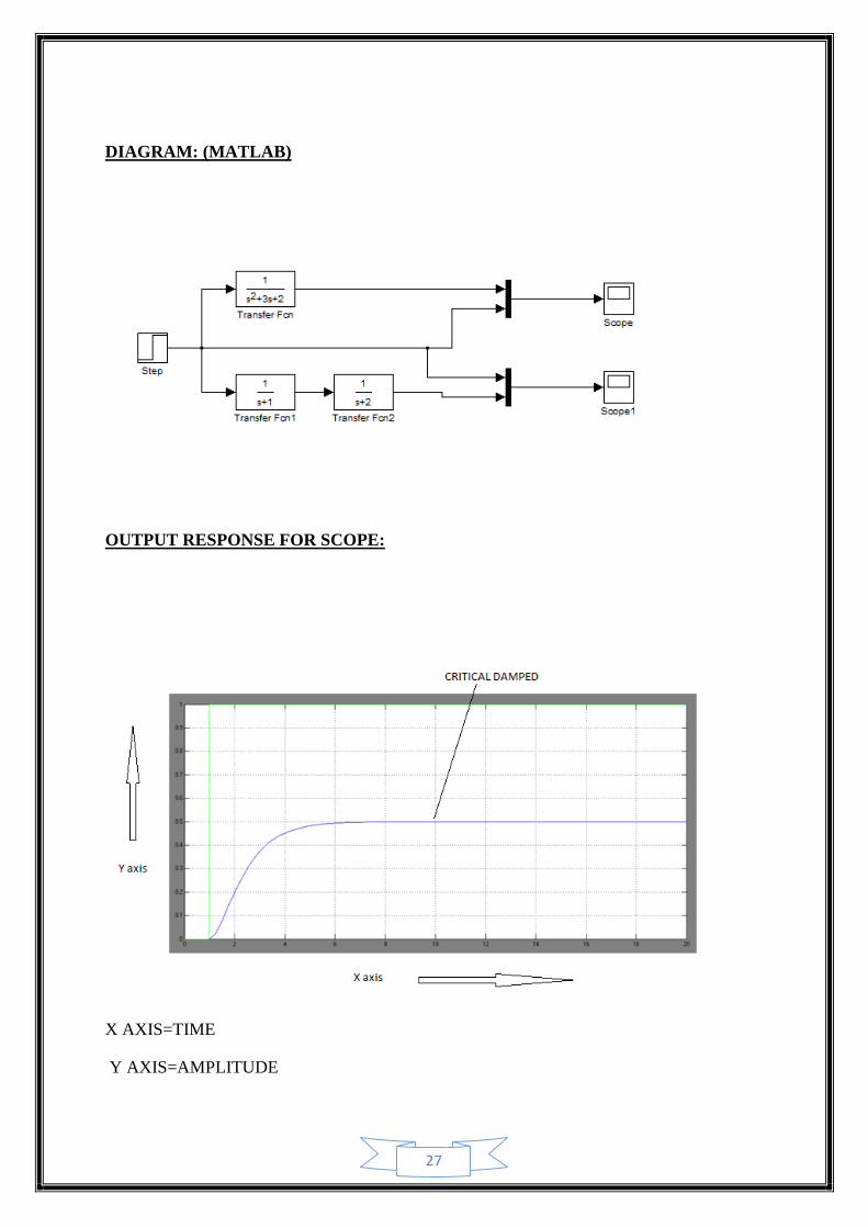
OUTPUT RESPONSE FOR SCOPE1:

X AXIS=TIME

Y AXIS=AMPLITUDE

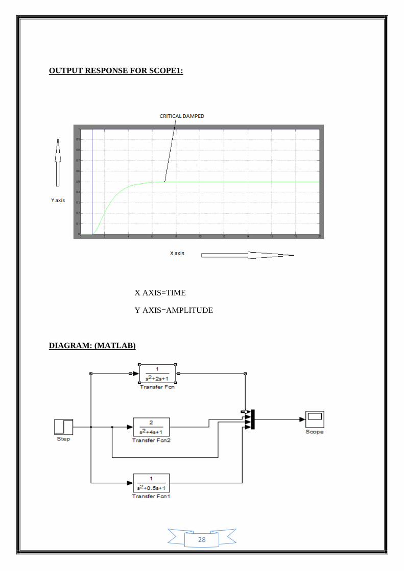
DIAGRAM: (MATLAB)

29

OUTPUT RESPONSE:

X AXIS=TIME

Y AXIS=AMPLITUDE

MATLAB: (DIAGRAM)

30

OUTPUT RESPONSE FOR SCOPE:

X AXIS=TIME

Y AXIS=AMPLITUDE

OUTPUT RESPONSE FOR SCOPE1:

X AXIS=TIME

Y AXIS=AMPLITUD

31

DIAGRAM (LABVIEW):

OUTPUT RESPONSE:

32

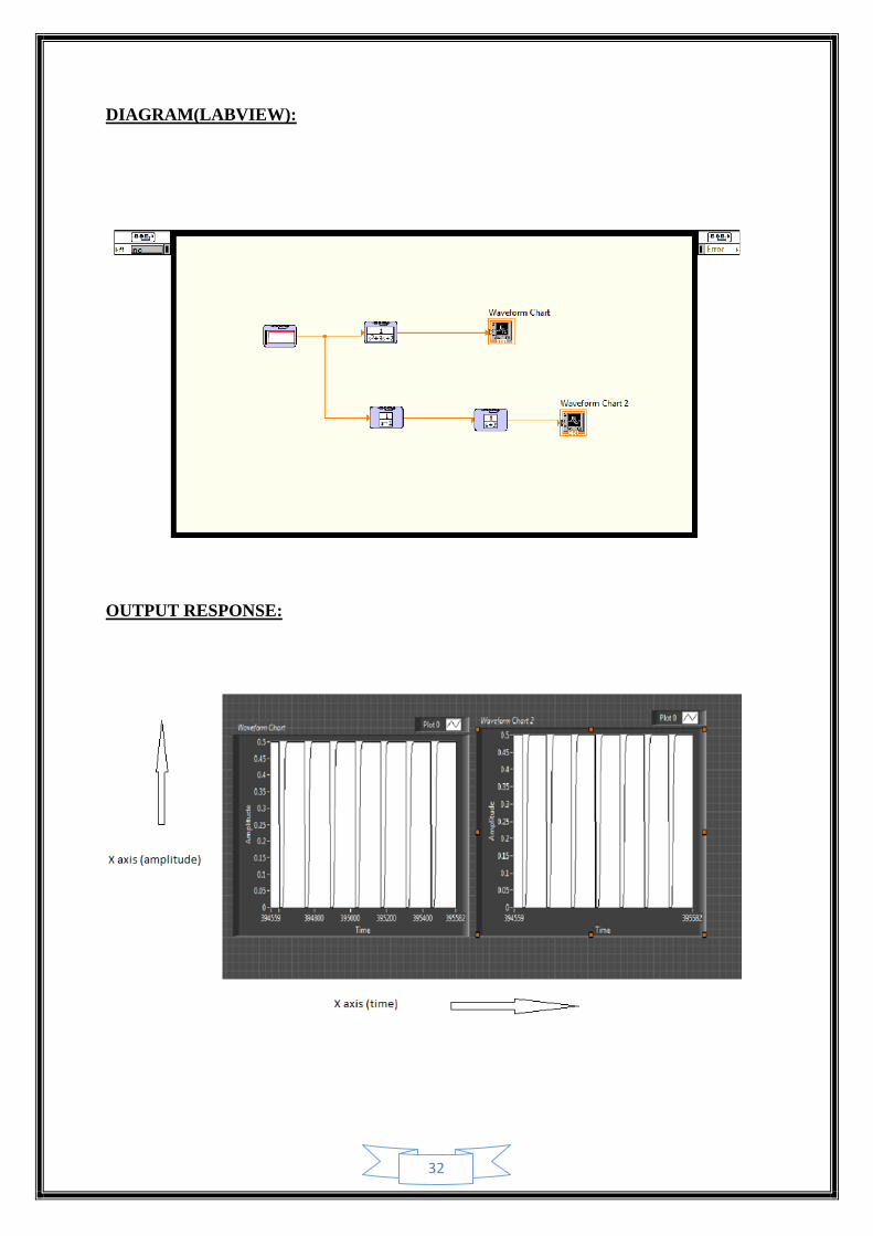
DIAGRAM(LABVIEW):

OUTPUT RESPONSE:

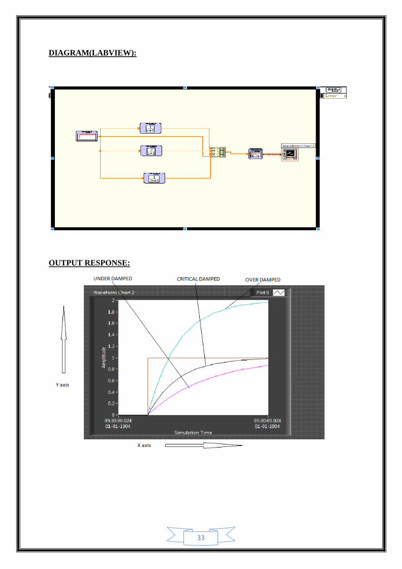
33

DIAGRAM(LABVIEW):

OUTPUT RESPONSE:

34

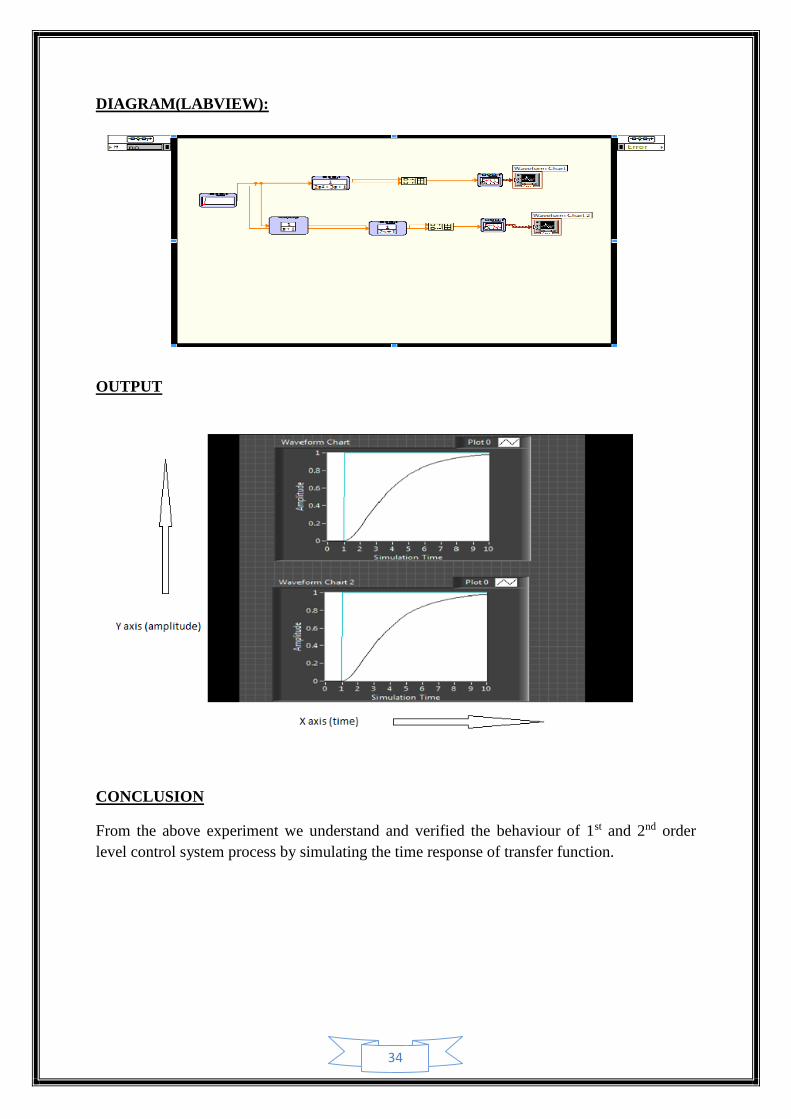
DIAGRAM(LABVIEW):

OUTPUT

CONCLUSION

From the above experiment we understand and verified the behaviour of 1st and 2nd order

level control system process by simulating the time response of transfer function.

35

EXPERIMENT-3

AIM OF THE EXPERIMENT:

To design a PID controller and compare response of the controller at the different point.

SOFTWARE REQUIREMENT:

MATLAB 2009b & LABVIEW 2010

THEORY: A proportional-integral-derivative controller (PID controller)is a

Common feedback loop component in industrial control systems (see also

Control theory).

The controller takes a measured value from a process or other apparatus

And compares it with a reference set point value. The difference (or “error" signal) is then

used to adjust some input to the process in order to bring the process' measured value back to

its desired set point. Unlike simpler controllers, the PID can adjust process outputs based on

the history and rate of change of the error signal, which gives more accurate and stable

control. PID controllers do not require advanced mathematics to design and can be easily

adjusted (or "tuned") to the desired application, unlike more complicated control algorithms

based on optimal control theory.

Control loop basics

Intuitively, the PID loop tries to automate what an intelligent operator with a gauge and a

control knob would do. The operator would read a gauge showing the output measurement of

a process, and use the knob to adjust the input of the process (the “action") until the process's

output measurement stabilizes at the desired value on the gauge. In older control literature

this adjustment process is called a "reset" action. The position of the needle on the gauge is a

"measurement", "process value" or “process variable". The desired value on the gauge is

called a "set point" (also called "set value"). The difference between the

Gauge’s needle and the set point is the "error".

A control loop consists of three parts:

1. Measurement by a sensor connected to the process (or the "plant"),

2. Decision in a controller element,

3. Action through an output device ("actuator") such as a control valve.

As the controller reads a sensor, it subtracts this measurement from the "setpoint" to

determine the "error". It then uses the error to calculate a correction to the process's input

variable (the "action") so that this correction will remove the error from the process's output

measurement.

In a PID loop, correction is calculated from the error in three ways: cancel out the current

error directly (Proportional), the amount of time the error has continued uncorrected

(Integral), and anticipate the future error from the rate of change of the error over time.

36

THEORY:

The PID loop adds positive corrections, removing error from the process's controllable

variable (its input).Differing terms are used in the process control industry: The "process

variable" is also called the "process's input" or "controller's

Output." The process's output is also called the "measurement" or "controller's input. “This

"up a bit, down a bit" movement of the process's input variable is how the PID loop

automatically finds the correct level of input for the process. "Turning the control knob"

reduces error, adjusting the process's input to keep the process's measured output at the set

point.

The error is found by subtracting the measured quantity from the set point.

"PID" is named after its three correcting calculations, whose sum constitutes the output of the

PID controller.

1. Proportional - To handle the immediate error, the error is multiplied by a constant P

(for "proportional"), and added to the controlled quantity. P is only valid in the band

over which a controller's output is proportional to the error of the system. For

example, for a heater, a controller with a proportional band of 10 °C and a set point of

20 °C would have an output of 100% at 10 °C, 50% at 15 °C and 10% at 19 °C. Note

that when the error is zero, a proportional controller's output is zero.

2. Integral - To learn from the past, the error is integrated (added up) over a period of

time, and then multiplied by a constant I (making an average), and added to the

controlled quantity. A simple proportional system either oscillates, moving back and

forth around the set point because there's nothing to remove the error when it

overshoots, or oscillates and/or stabilizes at a too low or too high value. By adding a

proportion of the average error to the process input, the average difference between

the process output and the set point is continually reduced. Therefore, eventually, a

well-tuned PID loop's process output will settle down at the set point. As an example,

a system that has a tendency for a lower value (heater in a cold environment), a

simple proportional system would oscillate and/or stabilize at a too low value because

when zero error is reached P is also zero thereby halting the system until it again is

too low.

3. Derivative - To handle the future, the first derivative (the slope of the error) over time

is calculated, and multiplied by another constant D, and also added to the controlled

quantity. The derivative term controls the response to a change in the system. The

larger the derivative term, the more rapidly the controller responds to changes in the

process's output. Its D term is the reason term is the reason a PID loop is also

sometimes called a "predictive controller." The D term is reduced when trying to

dampen a controller's response to short term changes. Practical controllers for slow

processes can even do without D term.

More technically, a PID loop can be characterized as a filter applied to a complex frequency-

domain system. This is useful in order to calculate whether it will actually reach a stable

value. If the values are chosen incorrectly, the controlled process input can oscillate, and the

process output may never stay at the set point.

37

A PID controller is called a PI, PD, or P controller in the absence of respective control

actions. It may be noted that EWMA (Exponential Weighted Moving Average) controller is

equivalent to PI controller.

The generic transfer function for a PID controller of the interacting form is

With C being a constant which depends on the bandwidth of the controlled system.

Traditionally, the output of the controller (i.e. the input to the process) is given by

Where Pcontrib, Icon rib, and Dcontrib are the feedback contributions from the PID

controller, defined below:

Where e(t) = Set point�� Measurement (t) is the error signal, and Kp, Ki, Kd are contents

that are used to tune the PID control loop:

1. Kp: Proportional Gain - Larger Kp typically means faster response since the larger

the error, the larger the feedback to compensate.

2. Ki: Integral Gain - Larger Ki implies steady state errors are eliminated quicker. The

trade-off is larger overshoot: any negative error integrated during transient response

must be integrated away by positive error before we reach steady state.

3. Kd: Derivative Gain - Larger Kd decreases overshoot, but slows down transient

response.

Normally the controller is implemented with the Kp gain applied to the Icontrib, and Dcontrib

terms as well in the following form;

Most standard tuning methods, such as Ziegler-Nichols and others, are based on this form, as

it reduces interaction. In this form, the Kip and Kdp gains relate only to dynamics of the

process, and the Kp (proportional gain) relates to the gain of the process. Often, one deals

with discrete time intervals instead of the continuity. Thus, the PID controller may also be

dealt with recursively:

38

39

CONCLUSION:

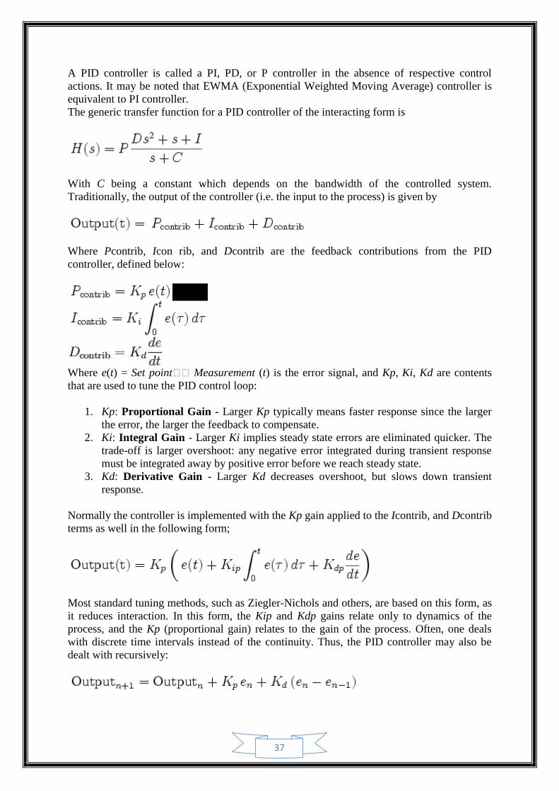
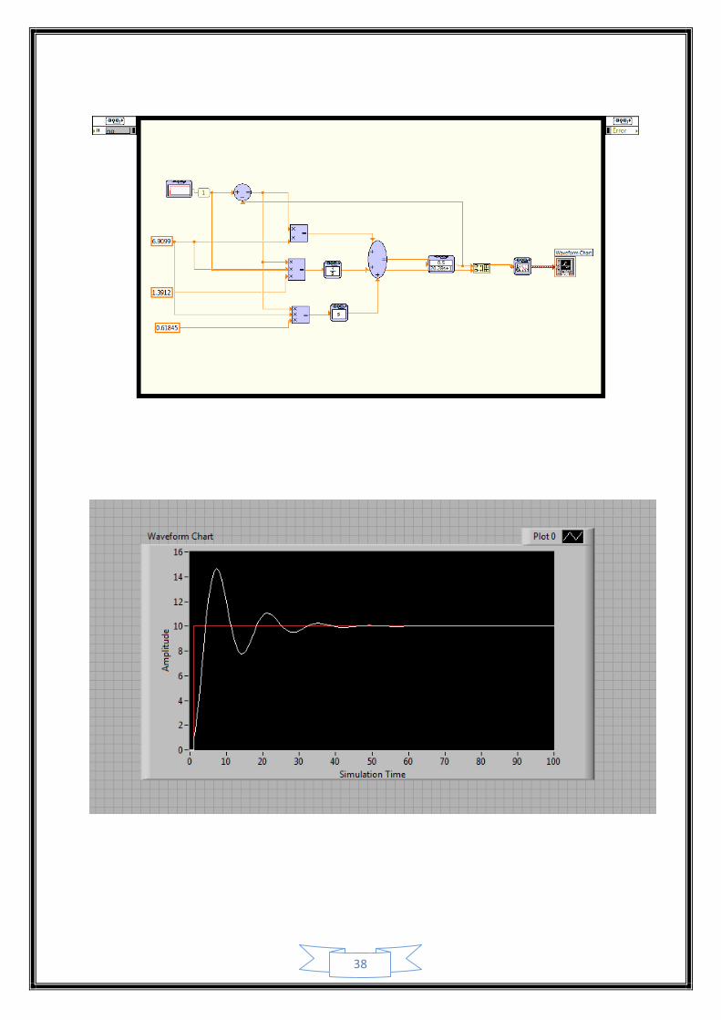
We have done the PID experiment using LABVIEW successfully.

40

EXPERIMENT-4

AIM OF THE EXPERIMENT:-

To design IMC (internal model control) with and without disturbance and Varity its response.

SOFTWARE REQUIRED:-

I. MATLAB R2009b

II. LABVIEW 2010

THEORY:-

Internal model control (IMC) has been the subject of intense research since about 1980.this

method of control which is based on an accurate model of process, leads to the design of the

control system i.e. stable and robust. A robust control system is one which maintains

satisfactory controls in spite of the changes in the dynamics of the process. In applying the

IMC method of control system design, the following information must be specified:

Process model

Model uncertainty

Type of input (step, ramp etc.)

Performance objective (integral square error, overshoot etc.)

In many industrial applications for control systems, one of the above item is available, with

the result that the system usually performs in ales than optimum manner. Determining the

mathematical model and its uncertainty can be a difficult task. When the process is not

sufficiently understood to obtain a mathematical model by applying fundamental principles,

one must obtain a model experimentally.

41

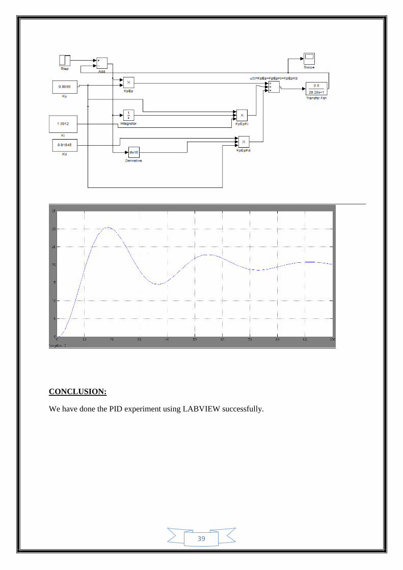
Design for IMC

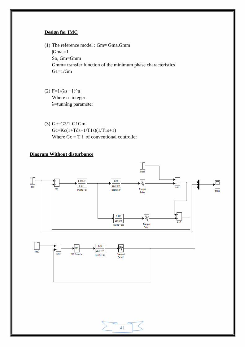
(1) The reference model : Gm= Gma.Gmm

|Gma|=1

So, Gm=Gmm

Gmm= transfer function of the minimum phase characteristics

G1=1/Gm

(2) F=1/(λs +1)^n

Where n=integer

λ=tunning parameter

(3) Gc=G2/1-G1Gm

Gc=Kc(1+Tds+1/T1s)(1/T1s+1)

Where Gc = T.f. of conventional controller

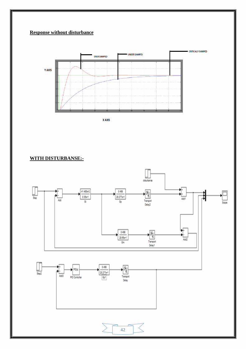
Diagram Without disturbance

42

Response without disturbance

WITH DISTURBANSE:-

43

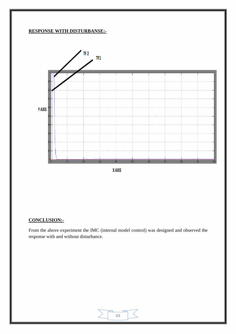
RESPONSE WITH DISTURBANSE:-

CONCLUSION:-

From the above experiment the IMC (internal model control) was designed and observed the

response with and without disturbance.

44

EXPERIMENT-5

AIM OF THE EXPERIMENT:

Design controller tuning methods using Lab VIEW.

APPARATUS REQUIRED:

Lab VIEW 2010 software.

THEORY:-

PID controllers are probably the most commonly used controller structures in industry. They

do, however, present some challenges to control and instrumentation engineers in the aspect

of tuning of the gains required for stability and good transient performance. There are several

prescriptive rules used in PID tuning. An example is that proposed by Ziegler and Nichols in

the 1940's and described in this note.

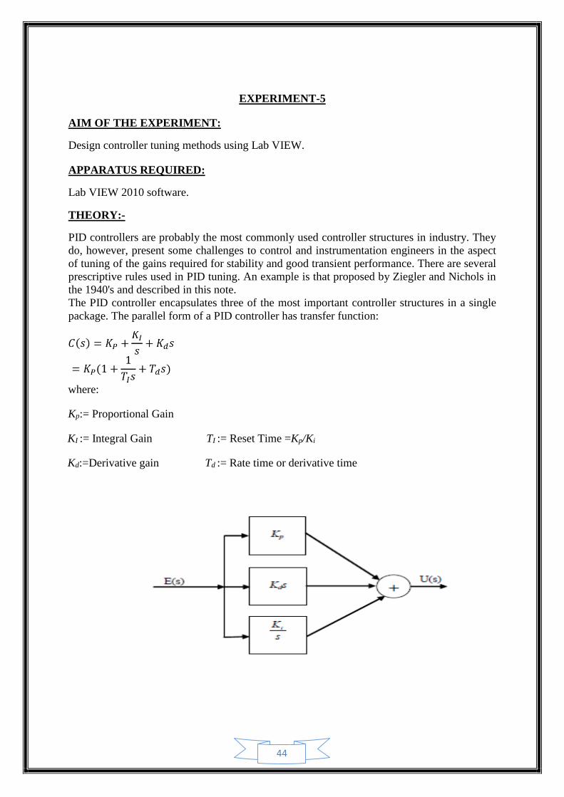
The PID controller encapsulates three of the most important controller structures in a single

package. The parallel form of a PID controller has transfer function:

where:

Kp:= Proportional Gain

KI := Integral Gain TI := Reset Time =Kp/Ki

Kd:=Derivative gain Td := Rate time or derivative time

45

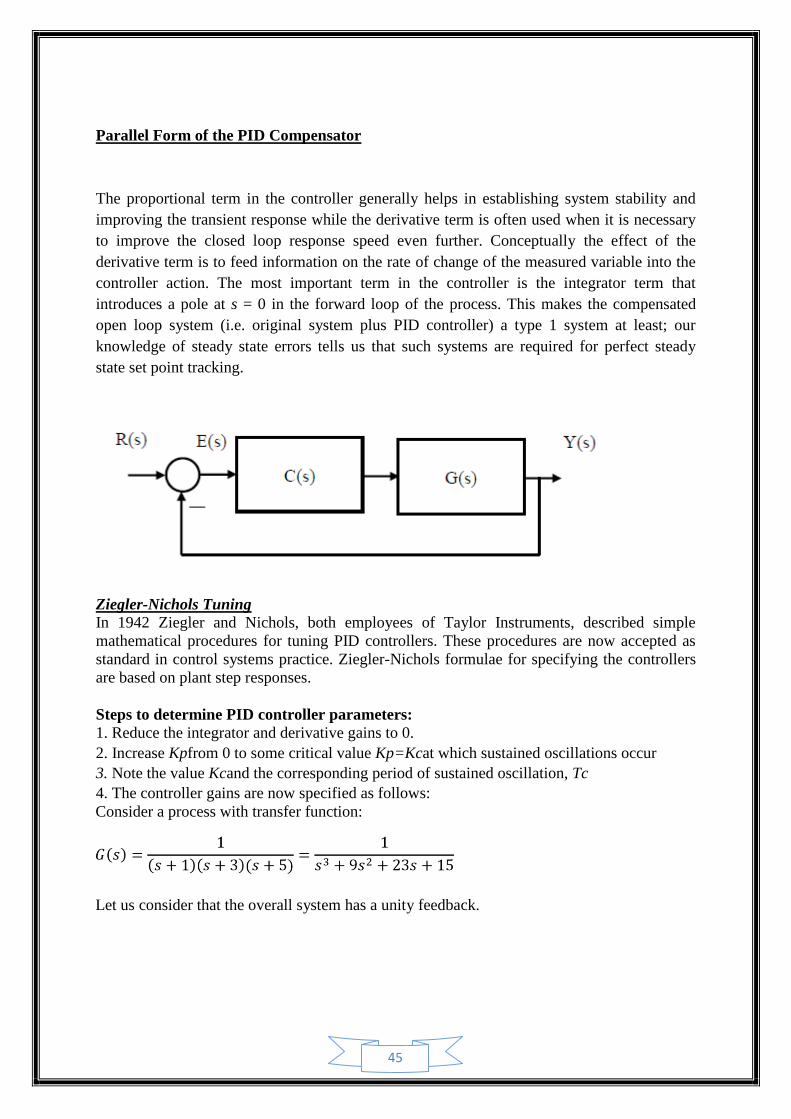
Parallel Form of the PID Compensator

The proportional term in the controller generally helps in establishing system stability and

improving the transient response while the derivative term is often used when it is necessary

to improve the closed loop response speed even further. Conceptually the effect of the

derivative term is to feed information on the rate of change of the measured variable into the

controller action. The most important term in the controller is the integrator term that

introduces a pole at s = 0 in the forward loop of the process. This makes the compensated

open loop system (i.e. original system plus PID controller) a type 1 system at least; our

knowledge of steady state errors tells us that such systems are required for perfect steady

state set point tracking.

Ziegler-Nichols Tuning

In 1942 Ziegler and Nichols, both employees of Taylor Instruments, described simple

mathematical procedures for tuning PID controllers. These procedures are now accepted as

standard in control systems practice. Ziegler-Nichols formulae for specifying the controllers

are based on plant step responses.

Steps to determine PID controller parameters:

1. Reduce the integrator and derivative gains to 0.

2. Increase Kpfrom 0 to some critical value Kp=Kcat which sustained oscillations occur

3. Note the value Kcand the corresponding period of sustained oscillation, Tc

4. The controller gains are now specified as follows:

Consider a process with transfer function:

Let us consider that the overall system has a unity feedback.

46

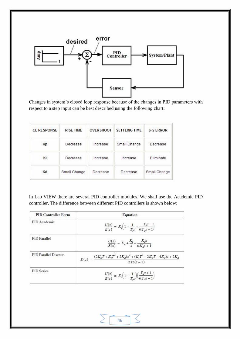
Changes in system’s closed loop response because of the changes in PID parameters with

respect to a step input can be best described using the following chart:

In Lab VIEW there are several PID controller modules. We shall use the Academic PID

controller. The difference between different PID controllers is shown below:

47

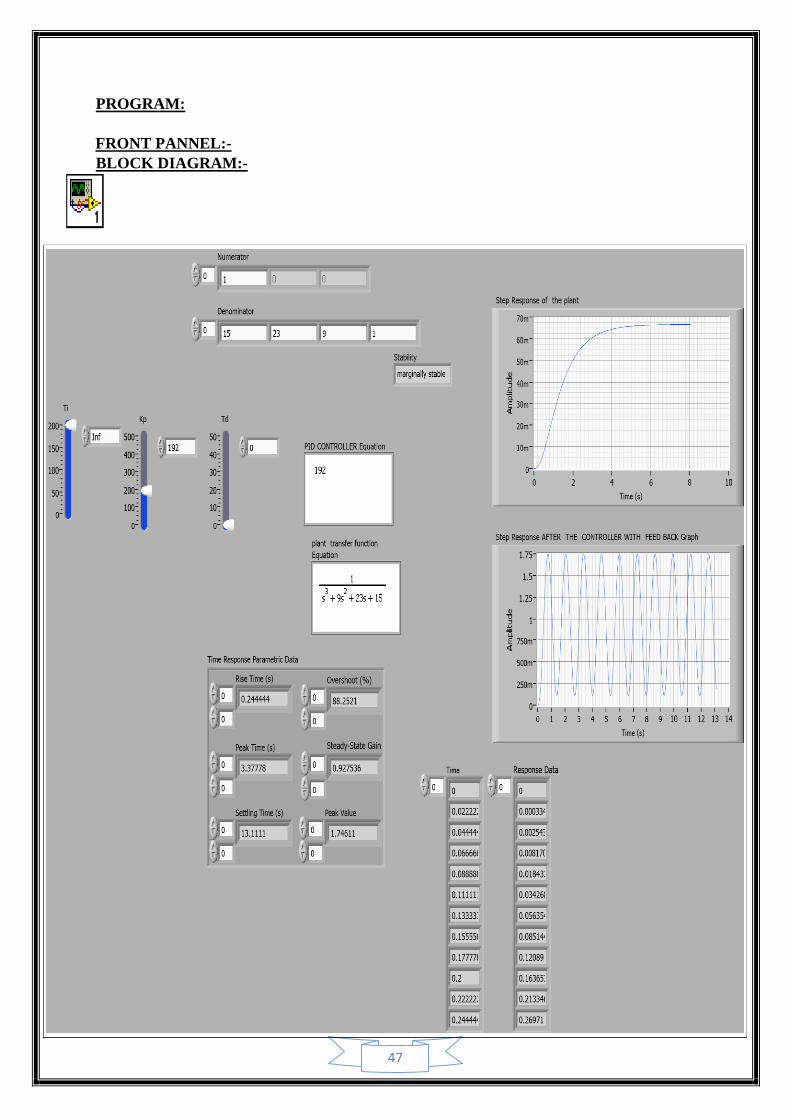
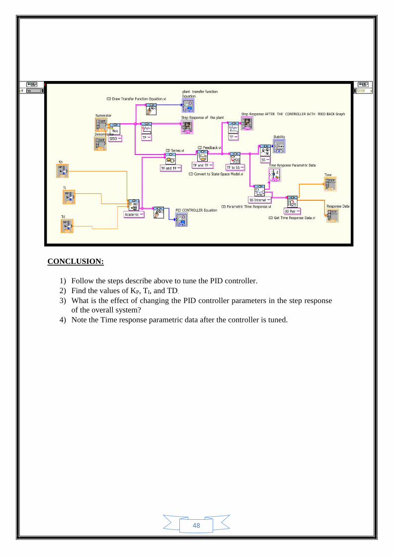
PROGRAM:

FRONT PANNEL:-

BLOCK DIAGRAM:-

48

CONCLUSION:

1) Follow the steps describe above to tune the PID controller.

2) Find the values of KP, TI, and TD.

3) What is the effect of changing the PID controller parameters in the step response

of the overall system?

4) Note the Time response parametric data after the controller is tuned.

49

EXPERIMENT-6

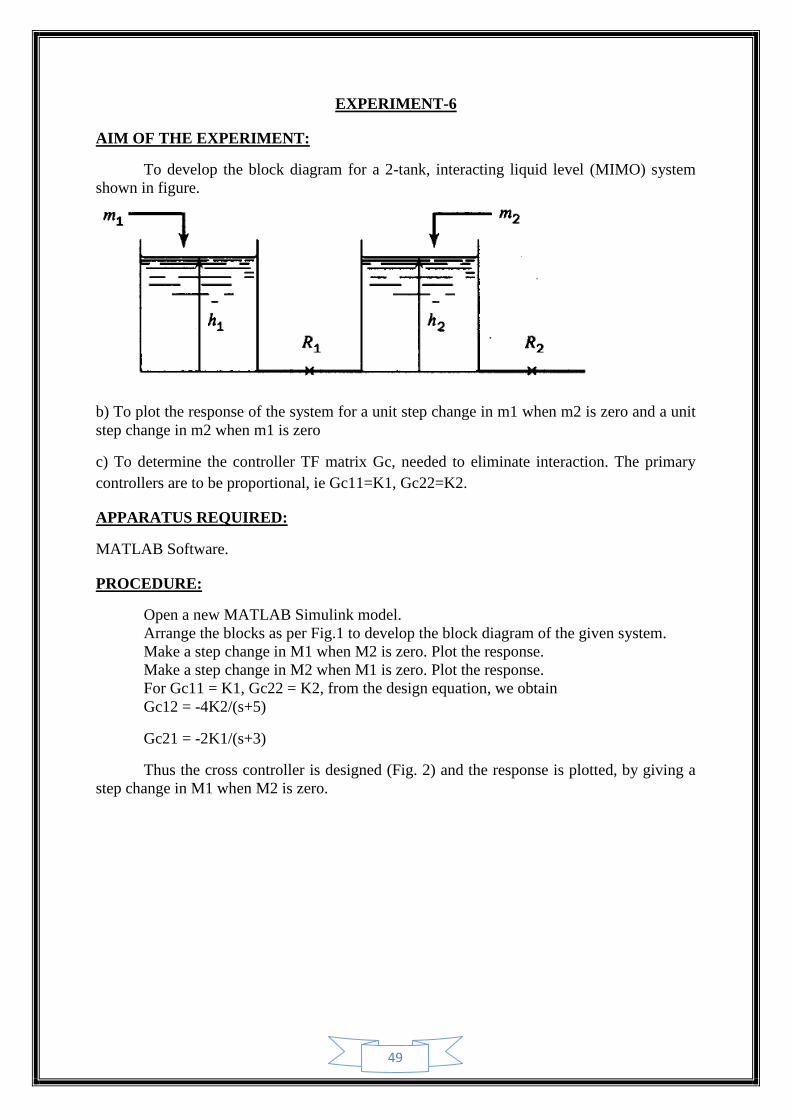
AIM OF THE EXPERIMENT:

To develop the block diagram for a 2-tank, interacting liquid level (MIMO) system

shown in figure.

b) To plot the response of the system for a unit step change in m1 when m2 is zero and a unit

step change in m2 when m1 is zero

c) To determine the controller TF matrix Gc, needed to eliminate interaction. The primary

controllers are to be proportional, ie Gc11=K1, Gc22=K2.

APPARATUS REQUIRED:

MATLAB Software.

PROCEDURE:

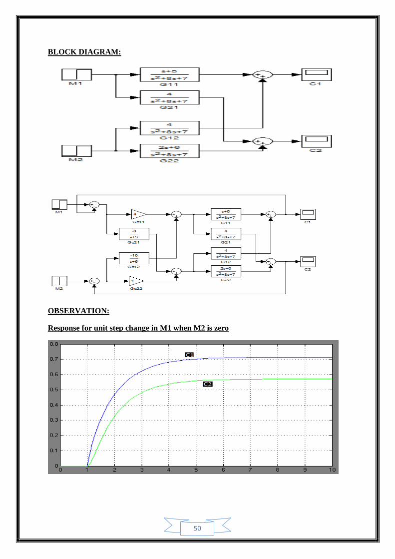
Open a new MATLAB Simulink model.

Arrange the blocks as per Fig.1 to develop the block diagram of the given system.

Make a step change in M1 when M2 is zero. Plot the response.

Make a step change in M2 when M1 is zero. Plot the response.

For Gc11 = K1, Gc22 = K2, from the design equation, we obtain

Gc12 = -4K2/(s+5)

Gc21 = -2K1/(s+3)

Thus the cross controller is designed (Fig. 2) and the response is plotted, by giving a

step change in M1 when M2 is zero.

50

BLOCK DIAGRAM:

OBSERVATION:

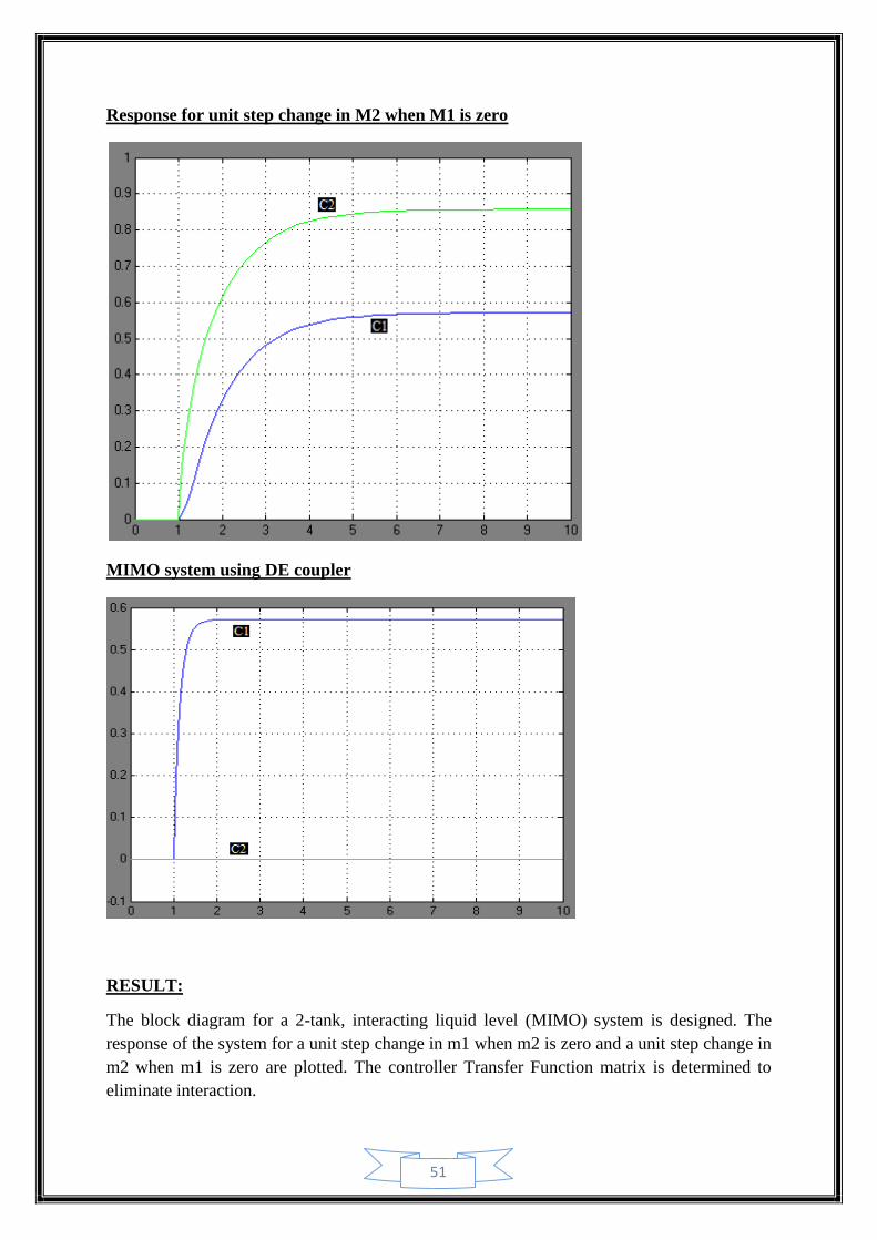
Response for unit step change in M1 when M2 is zero

51

Response for unit step change in M2 when M1 is zero

MIMO system using DE coupler

RESULT:

The block diagram for a 2-tank, interacting liquid level (MIMO) system is designed. The

response of the system for a unit step change in m1 when m2 is zero and a unit step change in

m2 when m1 is zero are plotted. The controller Transfer Function matrix is determined to

eliminate interaction.

52

EXPERIMENT-7

AIM OF THE EXPERIMENT:

a) To determine the values of all adjustable parameters of feed-forward and feed-back control

algorithm

b) To compare the response of the system for a unit step change in load for feed-back control

and feed-forward - feed-back control

APPARATUS REQUIRED:

MATLAB Software.

PROCEDURE:

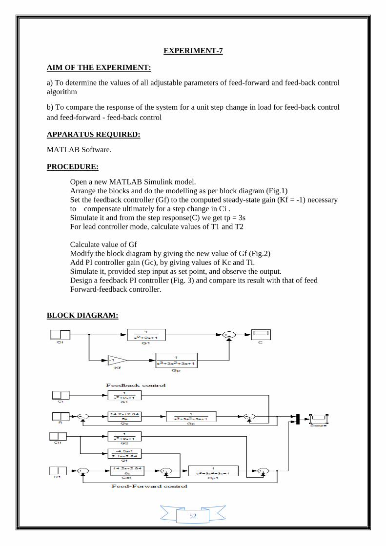
Open a new MATLAB Simulink model.

Arrange the blocks and do the modelling as per block diagram (Fig.1)

Set the feedback controller (Gf) to the computed steady-state gain (Kf = -1) necessary

to compensate ultimately for a step change in Ci .

Simulate it and from the step response(C) we get tp = 3s

For lead controller mode, calculate values of T1 and T2

Calculate value of Gf

Modify the block diagram by giving the new value of Gf (Fig.2)

Add PI controller gain (Gc), by giving values of Kc and Ti.

Simulate it, provided step input as set point, and observe the output.

Design a feedback PI controller (Fig. 3) and compare its result with that of feed

Forward-feedback controller.

BLOCK DIAGRAM:

53

CALCULATION:

tp = 3s

T1 = 1.5tp = 1.5 x 3 = 4.5s

T2 = 0.7tp = 0.7 x 3 = 2.1s

Gf(s) = Kf (T1s+1) / (T2s+1)

Kc = 2.84; Ti = 5s

OBSERVATION:

Feed-forward Control

Feed-forward – Feed-back Control Vs Feed-back Control

RESULT:

The design of feed forward controller is studied and the values of all adjustable parameters of

feed-forward and feed-back control algorithm are determined. Also, step response of this

system is improved, while comparing with feed-back control.

54

EXPERIMENT-8

AIM OF THE EXPERIMENT:

Design a cascade control scheme for the given system.

Show that the load response for the cascade control system is far superior to the load

response of the conventional control system.

Plot the responses to step change in set point for single-loop control and cascade

controller.

PROCEDURE:

Develop the closed-loop transfer functions for a cascade control system and for a

conventional control.

Arrange and connect the blocks as per the given block diagram.

Initialize the value of step time to zero.

Simulate the block and get the response.

Compare the responses of both conventional and cascade control.

BLOCK DIAGRAM:

55

OUTPUT RESPONSE:

LOAD RESPONSE:

RESPONSES TO STEP CHANGE IN SET POINT:

OBSERVATION:

Cascade control is especially useful in reducing the effect of a load disturbance that moves

through the control system slowly. The inner loop has the effect of reducing the lag in the

outer loop, with the result that the cascade system responds more quickly with a higher

frequency of oscillation.

RESULT:

Thus the conventional control and cascade control was designed and their output responses

were compared.

56

EXPERIMENT-9

AIM OF THE EXPERIMENT:-

To study and familiarize the Keyence and to familiarize with the ladder builder software for

PLC using some examples.

THEORY:-

Programmable Controller

The modern solution for the problem of how to provide discrete- state control is to use a

computer based device called a programmable controller (PC) or programmable logical

controller.

The move from relay logic controllers to computer based controllers was an obvious one

because

The input and output variables of discrete state control systems are binary in nature

just as with a computer.

Many of the control relays of the ladder diagrams can be replaced by software which

means less hardware failure.

It is very easy to make changes in the programmed sequence of events when it is only

a change in software.

Special software such as time delay action and counters are easy to form in software.

The semiconductor industry developed solid-state devices that can control high power

ac/dc in response to low level commands from a computer including SCR’s and TRIAC’s.

Basic Elements:-

There are three basic elements:

The processor

The input/output modules

Software

BLOCK DIAGRAM

Add i/o and cpu module block diagram.

Processor

The processor is a computer that executes a program to perform operation specified in a

ladder diagram or a set of Boolean equations. The processor performs arithmetic and logic

operations on input variable data and determines the proper state of the output variables. The

processor operates under a permanent supervisory operating system that directs overall

operations from data inputs and outputs to execute users program.

57

Programming unit

It is an external electronic package that is connected to the programmable controller when

programming occurs. The unit then transmits that program into the memory of programmable

controller

Processor:

It’s a computer that executes a program to perform the operations specified in a ladder

diagram. The processor performs the arithmetic and logic operations at the input variable data

and determines the proper state of output variable.

Input modules:

The input modules examine the state of physical switches and other input devices and their

state in to a form suitable for the processor. It is able to accommodate a number of inputs

called channels. Each channel is often equipped with an indicator light to show if the

particular input is ON or OFF.

Output modules:

They supply ac power to external devices such as motors, lights, solenoids and so on just as

required in the ladder diagram. Internally, the output module accepts a 1 or 0 input from the

processor and uses this to turn ON or OFF ac power control devices such as TRIAC.

In this state output relay is solid state relay. An output module will have one to several

channels per unit. Each channel is provided with an indicator light to show if the particular

channel is being driven ON or OFF.

Description:-

The KV-16 contains 16 I/O modules, 10 input modules and 6 output modules.KV-16 PLC is

programmed using software (via) ladder builder.PLC is using RC232C for communication

with PC.

Using above software all functions of PLC can be created on same principle as a relay

diagram. A KV ladder diagram can be created on same principle as a relay diagram.

Basic Operations using Ladder builder for KV editor:-

The editor offers following functions:

Creates ladder diagram using diversified instructions of ladder diagram language.

Performs editing function.

Register comments to contact and transfer, the converted diagram to PLC.

The maximum number of times that can be edited to one ladder diagrams is KV is 9999.

Entering and Detecting Symbols and Connection Lines:-

A ladder symbol is automatically entered when an instruction word is specified on by

entering as ‘0’ contact or an ‘a’ contact or a ‘b’ contact or a coil in the current cursor

position.

The following keys are available in KV.

58

No contact input (F3)

Normally closed contact input (Shift + F3)

Coil (F4)

Normally closed contact coil (Shift + F4)

Additional symbols can be selected by pressing F2 key.

PROCEDURE:-

1. Switch on PC.

2. From KV ladder menu select ‘Edit’ option

3. In edit select ‘new ladder file’

4. In that type a file name with extension

5. Select KV-16 type of PLC.

6. Then in the editor screen, enter the program.

7. To compile and simulate the entered program, select F1

8. In that select, compile + simulated

9. To simulate the program give appropriate input and observe the result

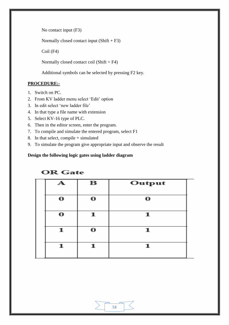
Design the following logic gates using ladder diagram

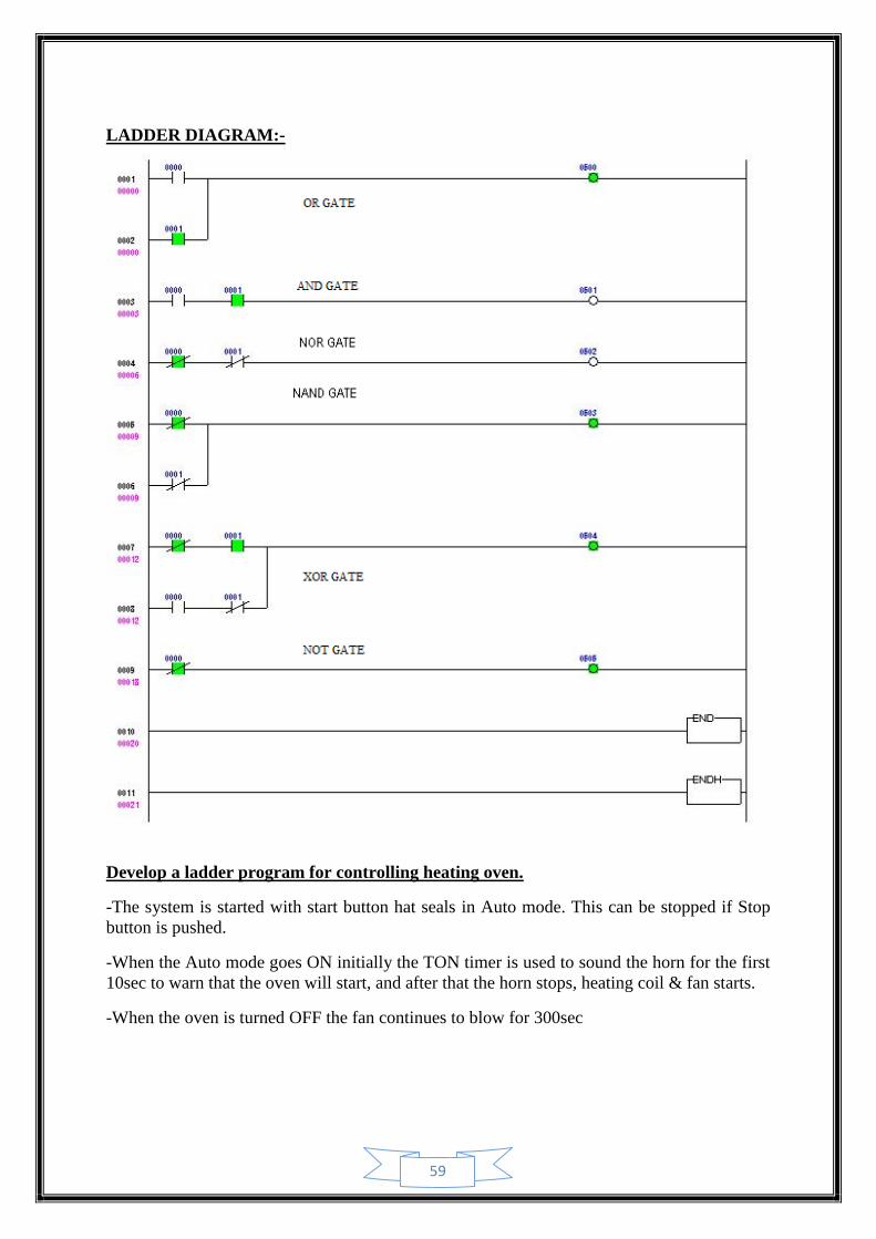
59

LADDER DIAGRAM:-

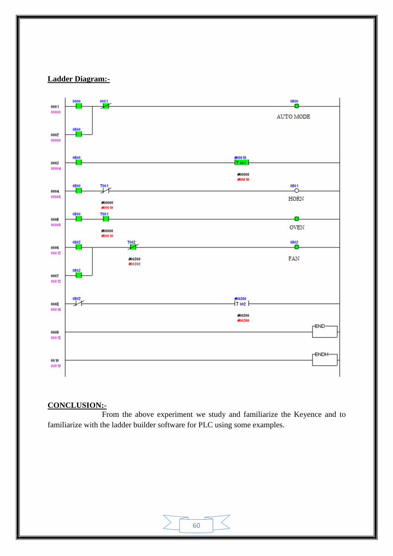
Develop a ladder program for controlling heating oven.

-The system is started with start button hat seals in Auto mode. This can be stopped if Stop

button is pushed.

-When the Auto mode goes ON initially the TON timer is used to sound the horn for the first

10sec to warn that the oven will start, and after that the horn stops, heating coil & fan starts.

-When the oven is turned OFF the fan continues to blow for 300sec

60

Ladder Diagram:-

CONCLUSION:-

From the above experiment we study and familiarize the Keyence and to

familiarize with the ladder builder software for PLC using some examples.

61

EXPERIMENT-10

AIM OF THE EXPERIMENT:-

To study and familiarize the Pico soft and to familiarize with the ladder builder software for

PLC using some examples.

PROCEDURE:-

1) Open the Pico soft software from the start menu.

2) Select a new file.

3) Go to any block and press enter. A window will pop up. Select input, output and timer

clicking on I, O and T respectively and also choose the members for naming the inputs and

outputs.

4) Using this method, implement the ladder logic for the given problem and save the file.

5) Compile and Run the program.

6) An input and output window will pop up. Now change the inputs as required to see the

desired output.

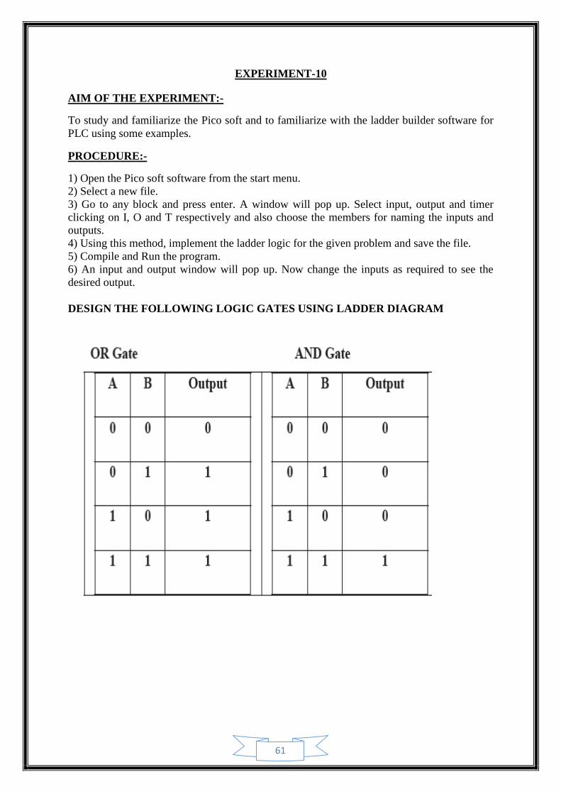
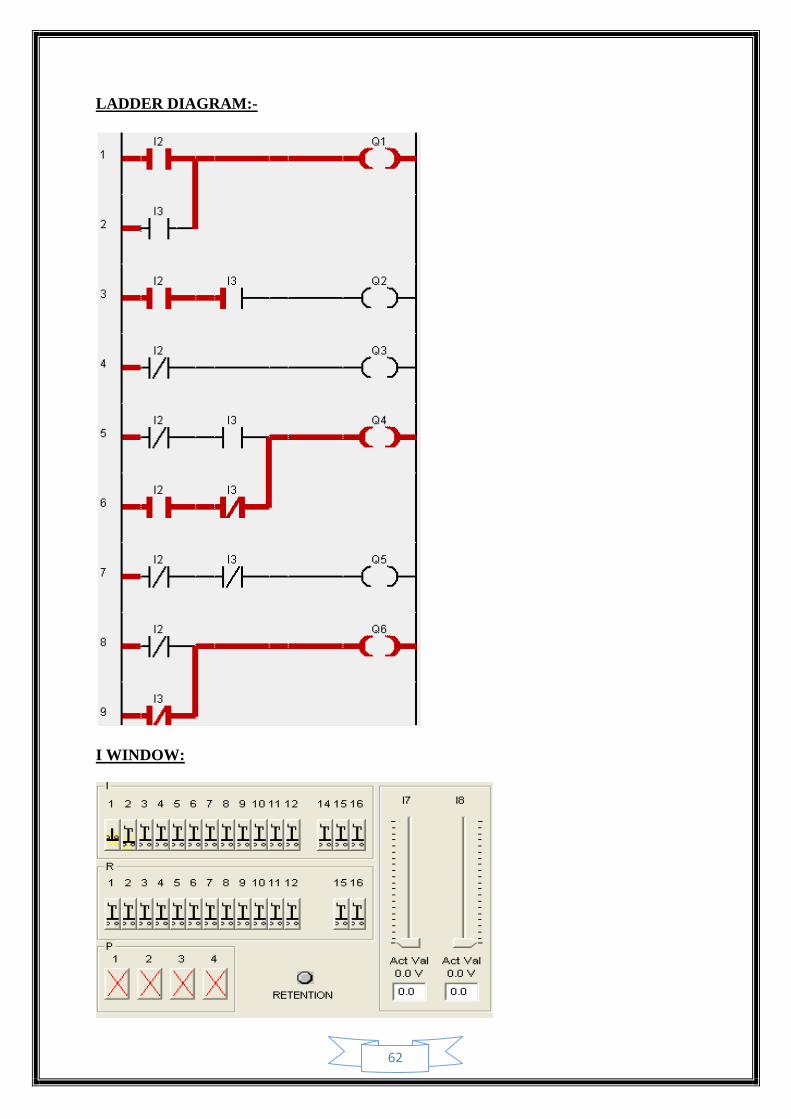
DESIGN THE FOLLOWING LOGIC GATES USING LADDER DIAGRAM

62

LADDER DIAGRAM:-

I WINDOW:

63

Q WINDOW:

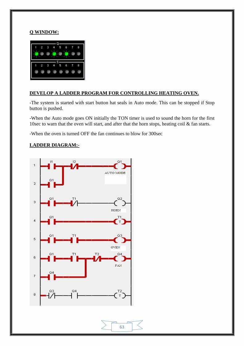
DEVELOP A LADDER PROGRAM FOR CONTROLLING HEATING OVEN.

-The system is started with start button hat seals in Auto mode. This can be stopped if Stop

button is pushed.

-When the Auto mode goes ON initially the TON timer is used to sound the horn for the first

10sec to warn that the oven will start, and after that the horn stops, heating coil & fan starts.

-When the oven is turned OFF the fan continues to blow for 300sec

LADDER DIAGRAM:-

64

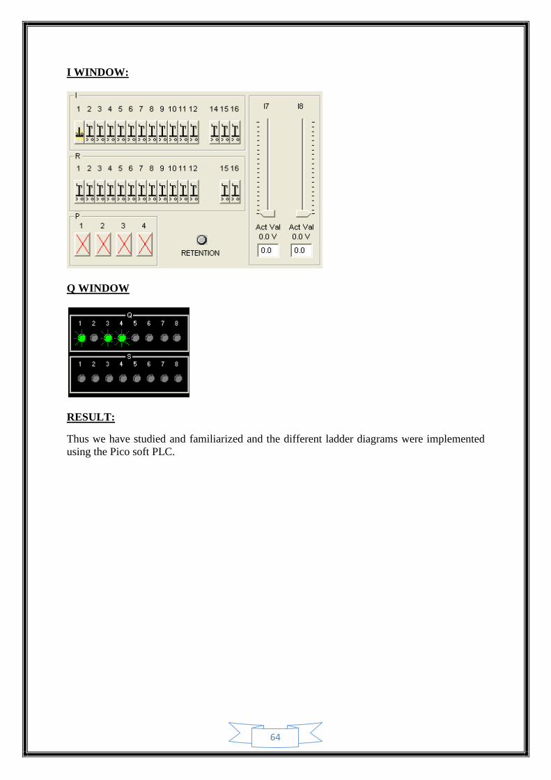
I WINDOW:

Q WINDOW

RESULT:

Thus we have studied and familiarized and the different ladder diagrams were implemented

using the Pico soft PLC.

65

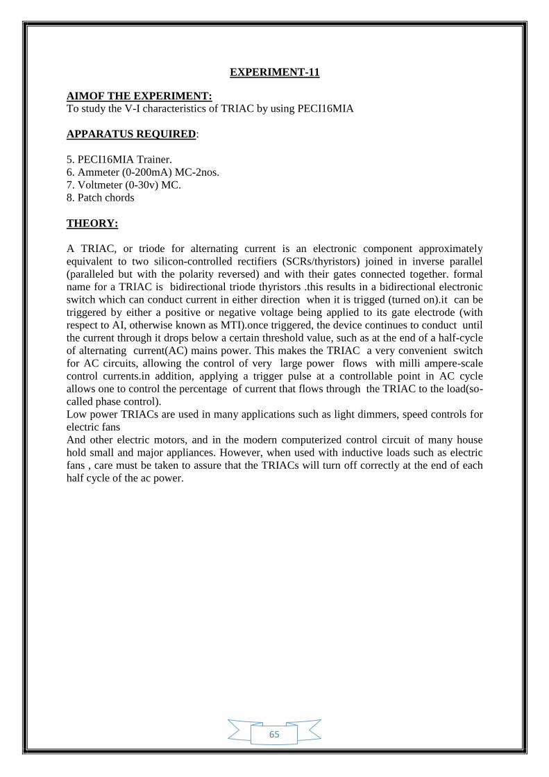
EXPERIMENT-11

AIMOF THE EXPERIMENT:

To study the V-I characteristics of TRIAC by using PECI16MIA

APPARATUS REQUIRED:

5. PECI16MIA Trainer.

6. Ammeter (0-200mA) MC-2nos.

7. Voltmeter (0-30v) MC.

8. Patch chords

THEORY:

A TRIAC, or triode for alternating current is an electronic component approximately

equivalent to two silicon-controlled rectifiers (SCRs/thyristors) joined in inverse parallel

(paralleled but with the polarity reversed) and with their gates connected together. formal

name for a TRIAC is bidirectional triode thyristors .this results in a bidirectional electronic

switch which can conduct current in either direction when it is trigged (turned on).it can be

triggered by either a positive or negative voltage being applied to its gate electrode (with

respect to AI, otherwise known as MTI).once triggered, the device continues to conduct until

the current through it drops below a certain threshold value, such as at the end of a half-cycle

of alternating current(AC) mains power. This makes the TRIAC a very convenient switch

for AC circuits, allowing the control of very large power flows with milli ampere-scale

control currents.in addition, applying a trigger pulse at a controllable point in AC cycle

allows one to control the percentage of current that flows through the TRIAC to the load(so-

called phase control).

Low power TRIACs are used in many applications such as light dimmers, speed controls for

electric fans

And other electric motors, and in the modern computerized control circuit of many house

hold small and major appliances. However, when used with inductive loads such as electric

fans , care must be taken to assure that the TRIACs will turn off correctly at the end of each

half cycle of the ac power.

66

67

CONNECTION PROCEDURE:

Connect the MT2 terminal of TRIAC is positive with respective to MT1 and gate

current also positive.

Connect the ammeter in anode terminal as indicated in the connection diagram.

Connect the ammeter in gate terminal as indicated in the connection diagram.

Connect the voltmeter in between TRIAC MT1 and MT2.

EXPERIMENTAL PROCEDURE:

1. Now switch on the 230 volt Ac supply.

2. Now vary the pot 3 and set the gate current IG.

3. Now slowly increase theMT1 and MT2 voltage by varying the pot 4 till the

TRIAC is turned on and note the voltage(VMT1),current (IF) readings as

shown in the table.

4. Now measure the break over voltage VB01.

5. Further increase the MT1-MT2 voltage and note the current IA.

6. Plot the Vf Vs If in a graph sheet.

TABULATION:

IG

=4.5MA(F.B)

IG =4.5MA(R.B)

SL NO VmT1 IA VmT1 If

1 3.3 0.3 -2.2 -2.0

2 3.5 0.4 -2.3 -1.9

3 4.4 0.5 -2.4 -1.7

4 5.3 0.6 -2.5 -1.6

5 5.8 0.6 -2.6 -1.5

6 6.8 0.7 -2.7 -1.4

7 7.7 0.8 -2.8 -1.3

8 8.7 0.9 -2.9 -1.1

9 9.1 0.9 -3.0 -1.0

10 9.9 1.0 -3.1 -0.92

68

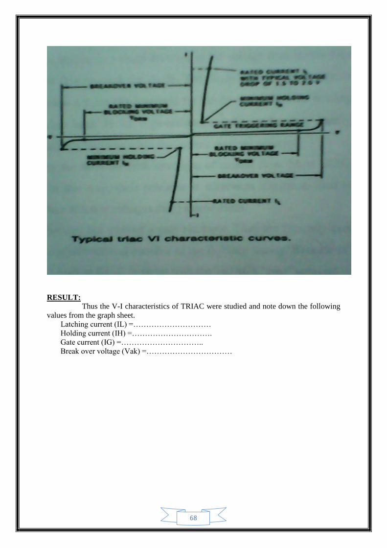
RESULT:

Thus the V-I characteristics of TRIAC were studied and note down the following

values from the graph sheet.

Latching current (IL) =…………………………

Holding current (IH) =………………………….

Gate current (IG) =…………………………..

Break over voltage (Vak) =……………………………

69

EXPERIMENT-12

AIM OF THE EXPERIMENT:

To study the v-i characteristics of SCR using PEC16MIA.

APPARATUS REQUIRED:

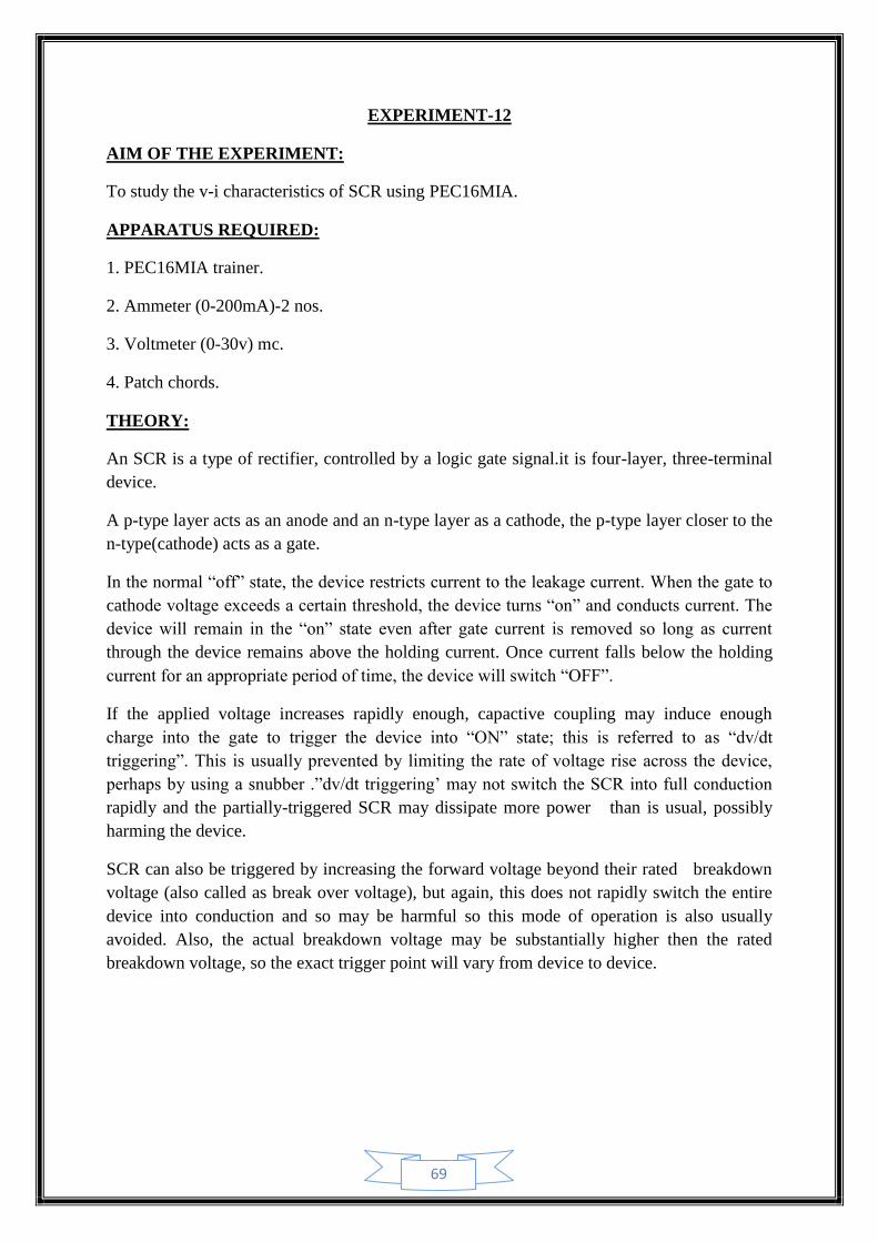
1. PEC16MIA trainer.

2. Ammeter (0-200mA)-2 nos.

3. Voltmeter (0-30v) mc.

4. Patch chords.

THEORY:

An SCR is a type of rectifier, controlled by a logic gate signal.it is four-layer, three-terminal

device.

A p-type layer acts as an anode and an n-type layer as a cathode, the p-type layer closer to the

n-type(cathode) acts as a gate.

In the normal “off” state, the device restricts current to the leakage current. When the gate to

cathode voltage exceeds a certain threshold, the device turns “on” and conducts current. The

device will remain in the “on” state even after gate current is removed so long as current

through the device remains above the holding current. Once current falls below the holding

current for an appropriate period of time, the device will switch “OFF”.

If the applied voltage increases rapidly enough, capactive coupling may induce enough

charge into the gate to trigger the device into “ON” state; this is referred to as “dv/dt

triggering”. This is usually prevented by limiting the rate of voltage rise across the device,

perhaps by using a snubber .”dv/dt triggering’ may not switch the SCR into full conduction

rapidly and the partially-triggered SCR may dissipate more power than is usual, possibly

harming the device.

SCR can also be triggered by increasing the forward voltage beyond their rated breakdown

voltage (also called as break over voltage), but again, this does not rapidly switch the entire

device into conduction and so may be harmful so this mode of operation is also usually

avoided. Also, the actual breakdown voltage may be substantially higher then the rated

breakdown voltage, so the exact trigger point will vary from device to device.

70

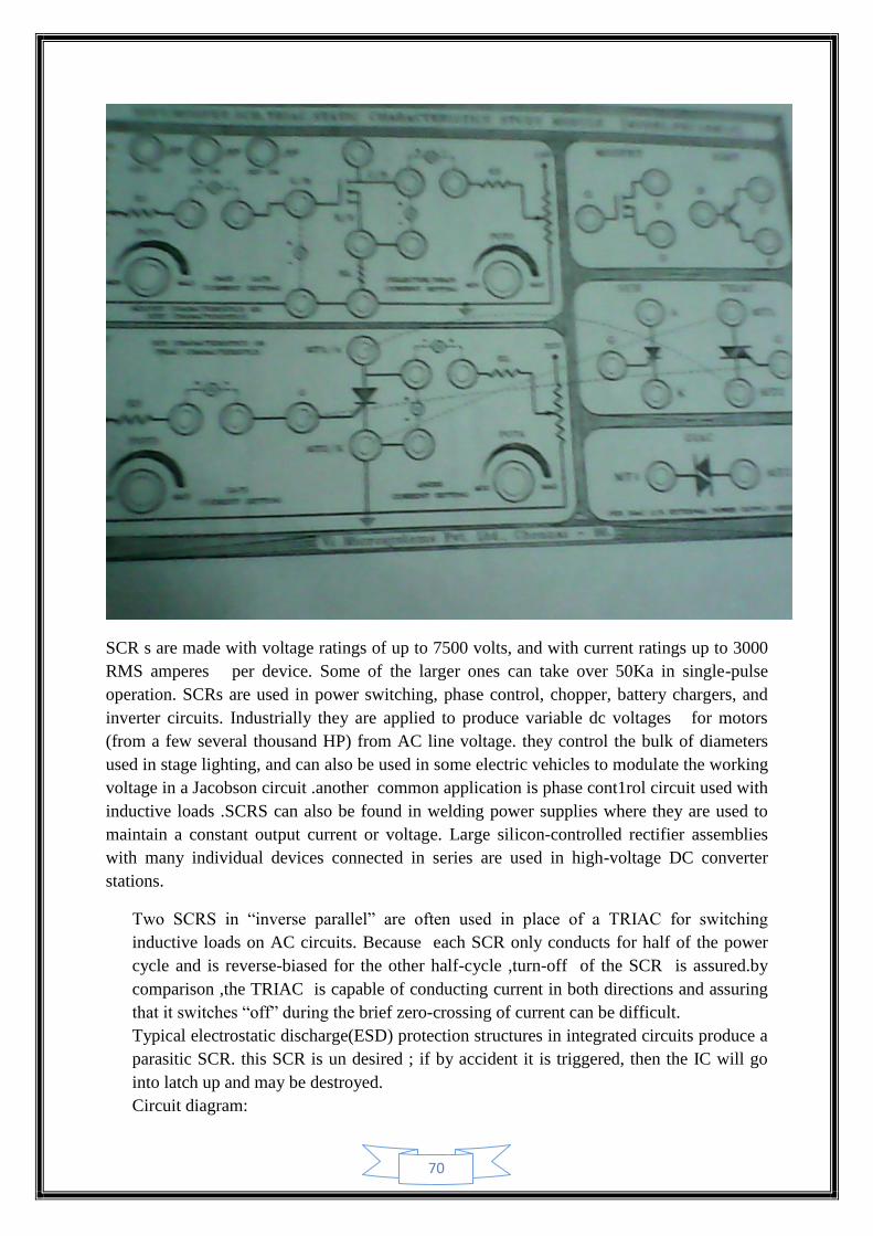
SCR s are made with voltage ratings of up to 7500 volts, and with current ratings up to 3000

RMS amperes per device. Some of the larger ones can take over 50Ka in single-pulse

operation. SCRs are used in power switching, phase control, chopper, battery chargers, and

inverter circuits. Industrially they are applied to produce variable dc voltages for motors

(from a few several thousand HP) from AC line voltage. they control the bulk of diameters

used in stage lighting, and can also be used in some electric vehicles to modulate the working

voltage in a Jacobson circuit .another common application is phase cont1rol circuit used with

inductive loads .SCRS can also be found in welding power supplies where they are used to

maintain a constant output current or voltage. Large silicon-controlled rectifier assemblies

with many individual devices connected in series are used in high-voltage DC converter

stations.

Two SCRS in “inverse parallel” are often used in place of a TRIAC for switching

inductive loads on AC circuits. Because each SCR only conducts for half of the power

cycle and is reverse-biased for the other half-cycle ,turn-off of the SCR is assured.by

comparison ,the TRIAC is capable of conducting current in both directions and assuring

that it switches “off” during the brief zero-crossing of current can be difficult.

Typical electrostatic discharge(ESD) protection structures in integrated circuits produce a

parasitic SCR. this SCR is un desired ; if by accident it is triggered, then the IC will go

into latch up and may be destroyed.

Circuit diagram:

71

Connection procedure:

Connect the SCR anode, cathode, gate terminal to SCR Characteristic circuit

Connect the ammeter in anode terminal as indicated in the connection diagram

Connect the ammeter is gate terminal.

Connect the voltmeter to across of anode and cathode terminal.

EXPERIMENTALPROCEDURE:

1. Switch on the 230v Ac supply.

2. Now vary the pot3 and set the gate current (IG) in the range of 4mA to 5 mA.

3. Now slowly increase the anode-cathode voltage (Vak) by varying the pot4 till the

thyristor get turned on, note down the ammeter (Ia), voltmeter (Vak) readings.

4. For various gate current take the reading and tabulate in Table I.

5. Plot vak vsia in a graph sheet.

6. After note down the max anode current remove the gate current by switch OFF the switch

Si.

72

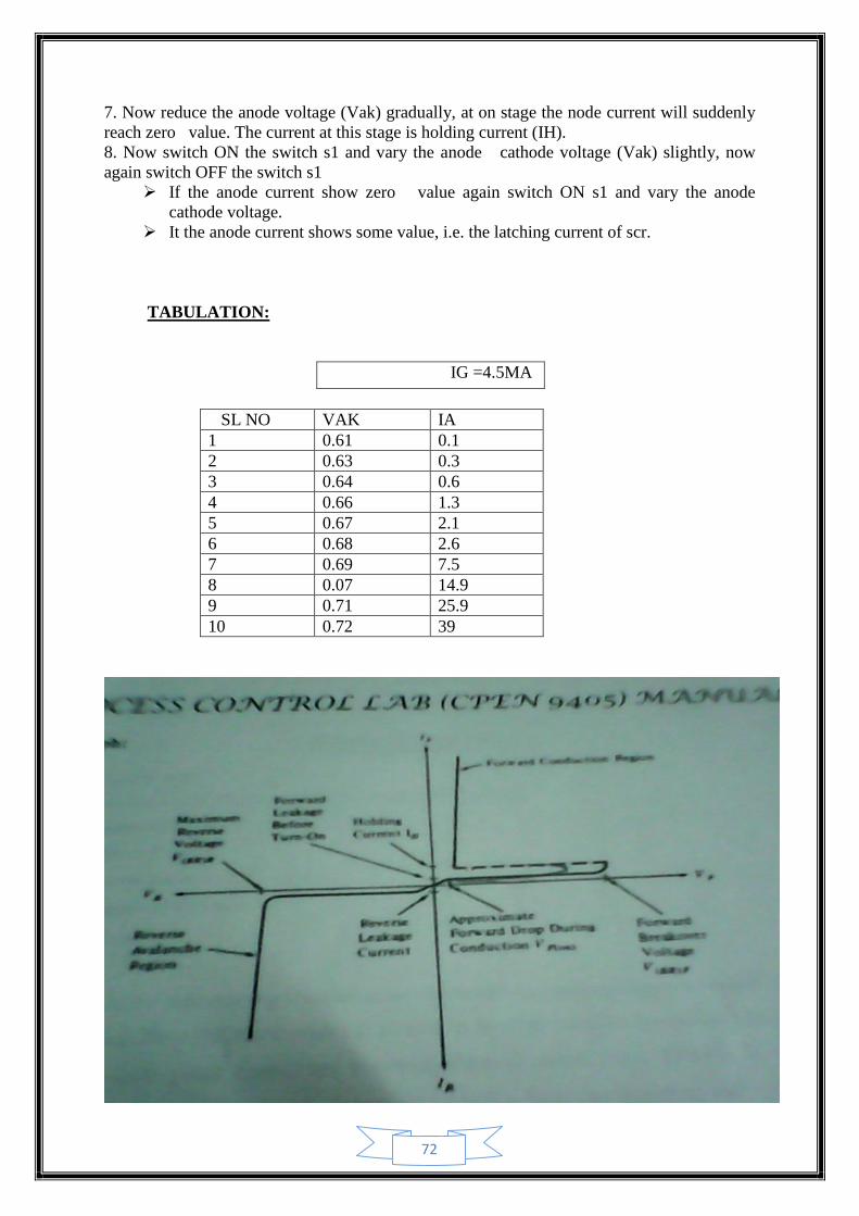
7. Now reduce the anode voltage (Vak) gradually, at on stage the node current will suddenly

reach zero value. The current at this stage is holding current (IH).

8. Now switch ON the switch s1 and vary the anode cathode voltage (Vak) slightly, now

again switch OFF the switch s1

If the anode current show zero value again switch ON s1 and vary the anode

cathode voltage.

It the anode current shows some value, i.e. the latching current of scr.

TABULATION:

IG =4.5MA

SL NO VAK IA

1 0.61 0.1

2 0.63 0.3

3 0.64 0.6

4 0.66 1.3

5 0.67 2.1

6 0.68 2.6

7 0.69 7.5

8 0.07 14.9

9 0.71 25.9

10 0.72 39

73

RESULT:

Thus the V-I characteristic of SCR were drawn and note the following values from the graph

sheet.

1. Latching current (IL) =----------------------.

2. Holding current (Ih) =----------------------.

3. Gate current (Ig) =--------------------------.

4. Break over voltage (Vak) =----------------.