Embed Size (px)
Citation preview

Chapter 2Chapter 2
Parallel Computing PlatformsParallel Computing Platforms
Dr. Muhammad Hanif Durad
Department of Computer and Information Sciences
Pakistan Institute Engineering and Applied Sciences
Some slides have bee adapted with thanks DANA PETCU'S athttp://web.info.uvt.ro/~petcu/index.html

Dr. Hanif Durad 2
Lecture Outline (1/2)
Implicit Parallelism: Trends in Microprocessor Architectures
Limitations of Memory System Performance Dichotomy of Parallel Computing Platforms Communication Model of Parallel Platforms

Dr. Hanif Durad 3
Lecture Outline (2/2)
Communication Costs in Parallel Machines Messaging Cost Models and Routing
Mechanisms Mapping Techniques Case Studies

Dr. Hanif Durad 4
Scope of Parallelism (1/2)
Conventional architectures coarsely comprise of a processor, memory system, and the datapath.
Each of these components present significant performance bottlenecks.
Parallelism addresses each of these components in significant ways.

Dr. Hanif Durad 5
Scope of Parallelism (2/2)
Different applications utilize different aspects of parallelism - e.g., data itensive applications utilize high aggregate throughput, server applications utilize high aggregate network bandwidth, and scientific applications typically utilize high processing and memory system performance.
It is important to understand each of these performance bottlenecks.

Dr. Hanif Durad 6
2.1 Implicit Parallelism: Trends in Microprocessor Architectures (1/2)
Microprocessor clock speeds have posted impressive gains over the past two decades (two to three orders of magnitude).
Higher levels of device integration have made available a large number of transistors.
The question of how best to utilize these resources is an important one.
Dr. Hanif Durad 7
2.1 Implicit Parallelism: Trends in Microprocessor Architectures (2/2)
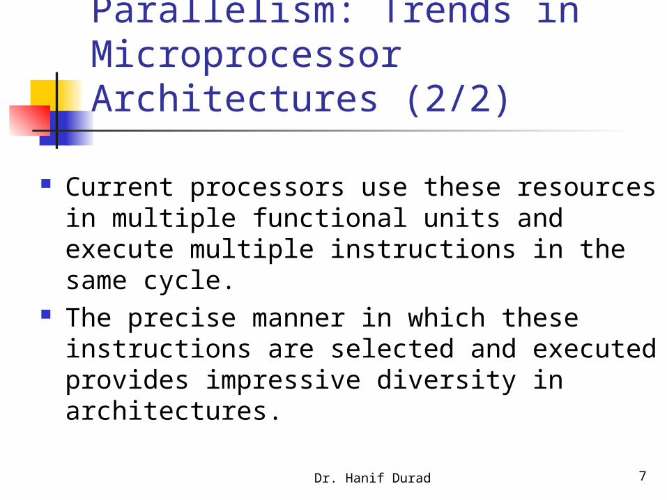
Current processors use these resources in multiple functional units and execute multiple instructions in the same cycle.
The precise manner in which these instructions are selected and executed provides impressive diversity in architectures.

Dr. Hanif Durad 8
2.1.1 Pipelining and Superscalar Execution (1/4)
Pipelining overlaps various stages of instruction execution to achieve performance.
At a high level of abstraction, an instruction can be executed while the next one is being decoded and the next one is being fetched.
This is akin to an assembly line for manufacture of cars.

Dr. Hanif Durad 9
Pipelining and Superscalar Execution (2/4)
Pipelining, however, has several limitations. The speed of a pipeline is eventually limited by
the slowest stage. For this reason, conventional processors rely
on very deep pipelines (20 stage pipelines in state-of-the-art Pentium processors).

Dr. Hanif Durad 10
Pipelining and Superscalar Execution (3/4)
However, in typical program traces, every 5-6th instruction is a conditional jump! This requires very accurate branch prediction.
The penalty of a misprediction grows with the depth of the pipeline, since a larger number of instructions will have to be flushed.
One simple way of alleviating these bottlenecks is to use multiple pipelines.
The question then becomes one of selecting these instructions

Dr. Hanif Durad 11
Superscalar Execution: An Example (2.1)
(a) Three different code fragments for a list of four numbers

Dr. Hanif Durad 12
Superscalar Execution: An Example
Execution Schedule for code fragment (i) above

Dr. Hanif Durad 13
Superscalar Execution: An Example
In the above example, there is some wastage of resources due to data dependencies.
The example also illustrates that different instruction mixes with identical semantics can take significantly different execution time.
load R1, @1000 and add R1, @1004etc.

Dr. Hanif Durad 14
Pipelining Execution
Instruction i IF ID EX WB
IF ID EX WB
IF ID EX WB
IF ID EX WB
IF ID EX WB
Instruction i+1
Instruction i+2
Instruction i+3
Instruction i+4
Instruction # 1 2 3 4 5 6 7 8
Cycles
IF: Instruction fetch ID : Instruction decodeEX : Execution WB : Write back

Dr. Hanif Durad 15
Super-Scalar Execution
Instruction type31 2 4 5 6 7
Cycles
Integer IF ID EX WB
Floating point IF ID EX WB
Integer
Floating point
Integer
Floating point
Integer
Floating point
IF ID EX WB
IF ID EX WB
IF ID EX WB
IF ID EX WB
IF ID EX WB
IF ID EX WB
2-issue super-scalar machine
Dr. Hanif Durad 16
Superscalar Execution
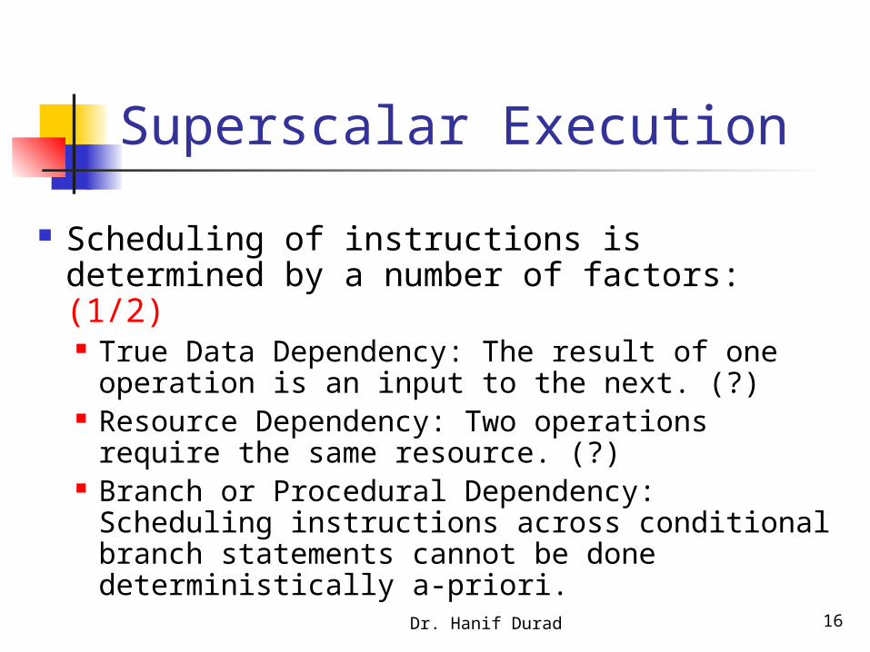
Scheduling of instructions is determined by a number of factors: (1/2) True Data Dependency: The result of one operation is
an input to the next. (?) Resource Dependency: Two operations require the
same resource. (?) Branch or Procedural Dependency: Scheduling
instructions across conditional branch statements cannot be done deterministically a-priori.

Dr. Hanif Durad 17
Superscalar Execution
Scheduling of instructions is determined by a number of factors: (2/2) The scheduler, a piece of hardware looks at a large
number of instructions in an instruction queue and selects appropriate number of instructions to execute concurrently based on these factors.
The complexity of this hardware is an important constraint on superscalar processors.

Dr. Hanif Durad 18
Legend for next slide taken from CA course
Fetch Instruction (FI) Decode Instruction (DI) Calculate operands (i.e. EAs) (CO) Fetch Operands (FO) Execute Instructions (EI) Write Operands (WO)
Overlap these operations

Dr. Hanif Durad 19
Timing Diagram for Instruction Pipeline Operation

Dr. Hanif Durad 20
The Effect of a Conditional Branch on Instruction Pipeline Operation No inst completed
in these 4 cycles
Know about conditional jump
Must be flushed

Dr. Hanif Durad 21
Superscalar Execution: Issue Mechanisms
In the simpler model, instructions can be issued only in the order in which they are encountered. That is, if the second instruction cannot be issued because it has a data dependency with the first, only one instruction is issued in the cycle. This is called in-order issue.

Dr. Hanif Durad 22
Superscalar Execution: Issue Mechanisms
In a more aggressive model, instructions can be issued out-of-order. In this case, if the second instruction has data dependencies with the first, but the third instruction does not, the first and third instructions can be co-scheduled. This is also called dynamic instruction issue.
Performance of in-order issue is generally limited.
Dr. Hanif Durad 23
Superscalar Execution: Efficiency Considerations
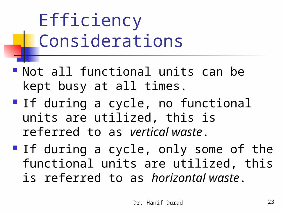
Not all functional units can be kept busy at all times.
If during a cycle, no functional units are utilized, this is referred to as vertical waste.
If during a cycle, only some of the functional units are utilized, this is referred to as horizontal waste.

Dr. Hanif Durad 24
Superscalar Execution: An Example
Hardware utilization trace for schedule in (b).

Dr. Hanif Durad 25
Superscalar Execution: Efficiency Considerations
Due to limited parallelism in typical instruction traces, dependencies, or the inability of the scheduler to extract parallelism, the performance of superscalar processors is eventually limited.
Conventional microprocessors typically support four-way superscalar execution.

Dr. Hanif Durad 26
2.1.2 Very Long Instruction Word (VLIW) Processors
The hardware cost and complexity of the superscalar scheduler is a major consideration in processor design.
To address this issues, VLIW processors rely on compile time analysis to identify and bundle together instructions that can be executed concurrently.

Dr. Hanif Durad 27
Very Long Instruction Word (VLIW) Processors
These instructions are packed and dispatched together, and thus the name very long instruction word.
This concept was used with some commercial success in the Multiflow Trace machine (circa 1984).
Variants of this concept are employed in the Intel IA64 processors.

Dr. Hanif Durad 28
VLIW Processors: Considerations
Issue hardware is simpler. Compiler has a bigger context from which to
select co-scheduled instructions. Compilers, however, do not have runtime
information such as cache misses. Scheduling is, therefore, inherently conservative.
Branch and memory prediction is more difficult.

Dr. Hanif Durad 29
VLIW Processors: Considerations
Very sensitive to the compilers' ability to detect data and resource dependencies and read and write hazards, and to schedule instructions for maximum parallelism.
A number of techniques such as loop unrolling, speculative execution, branch prediction are critical.
Typical VLIW processors are limited to 4-way to 8-way parallelism.

Dr. Hanif Durad 30

Dr. Hanif Durad 31
2.2 Limitations of Memory System Performance
Memory system, and not processor speed, is often the bottleneck for many applications.
Memory system performance is largely captured by two parameters, latency and bandwidth.
Latency is the time from the issue of a memory request to the time the data is available at the processor.
Bandwidth is the rate at which data can be pumped to the processor by the memory system.

Dr. Hanif Durad 32
Memory System Performance: Bandwidth and Latency
It is very important to understand the difference between latency and bandwidth.
Consider the example of a fire-hose. If the water comes out of the hose two seconds after the hydrant is turned on, the latency of the system is two seconds.
Once the water starts flowing, if the hydrant delivers water at the rate of 5 gallons/second, the bandwidth of the system is 5 gallons/second.
If you want immediate response from the hydrant, it is important to reduce latency.
If you want to fight big fires, you want high bandwidth.

Dr. Hanif Durad 33
Memory Latency: An Example (2.2)
Consider a processor operating at 1 GHz (1 ns clock) connected to a DRAM with a latency of 100 ns (no caches). Assume that the processor has two multiply-add units and is capable of executing four instructions in each cycle of 1 ns. The following observations follow: The peak processor rating is 4 GFLOPS. Since the memory latency is equal to 100 cycles and
block size is one word, every time a memory request is made, the processor must wait 100 cycles before it can process the data.

Dr. Hanif Durad 34

Dr. Hanif Durad 35
Memory Latency: An Example
On the above architecture, consider the problem of computing a dot-product of two vectors. A dot-product computation performs one multiply-add
on a single pair of vector elements, i.e., each floating point operation requires one data fetch.
It follows that the peak speed of this computation is limited to one floating point operation every 100 ns, or a speed of 10 MFLOPS, a very small fraction of the peak processor rating! Solution ?

Dr. Hanif Durad 36
2.2.1 Improving Effective Memory Latency Using Caches
Caches are small and fast memory elements between the processor and DRAM.
This memory acts as a low-latency high-bandwidth storage. If a piece of data is repeatedly used, the effective latency of this
memory system can be reduced by the cache. The fraction of data references satisfied by the cache is called the
cache hit ratio of the computation on the system. Cache hit ratio achieved by a code on a memory system often
determines its performance.

Traditional (ISA) (with cache)

Dr. Hanif Durad 38
Impact of Caches: Example (2.3)
Consider the architecture from the previous example. In this case, we introduce a cache of size 32 KB with a latency of 1 ns or one cycle. We use this setup to multiply two matrices A and B of dimensions 32 × 32. We have carefully chosen these numbers so that the cache is large enough to store matrices A and B, as well as the result matrix C.

Dr. Hanif Durad 39
Impact of Caches: Example (continued)
The following observations can be made about the problem: Fetching the two matrices into the cache corresponds to fetching
2K words, which takes approximately 200 µs. Multiplying two n × n matrices takes 2n3 operations. For our
problem, this corresponds to 64K operations, which can be performed in 16K cycles (or 16 µs) at four instructions per cycle.
The total time for the computation is therefore approximately the sum of time for load/store operations and the time for the computation itself, i.e., 200 + 16 µs.
This corresponds to a peak computation rate of 64K/216 or 303 MFLOPS.

Dr. Hanif Durad 40
Impact of Caches
Repeated references to the same data item correspond to temporal locality.
In our example, we had O(n2) data accesses and O(n3) computation. This asymptotic difference makes the above example particularly desirable for caches.
• Data reuse is critical for cache performance.

Dr. Hanif Durad 41
2.2.2 Impact of Memory Bandwidth
Memory bandwidth is determined by the bandwidth of the memory bus as well as the memory units.
Memory bandwidth can be improved by increasing the size of memory blocks.
The underlying system takes l time units (where l is the latency of the system) to deliver b units of data (where b is the block size).

Dr. Hanif Durad 42
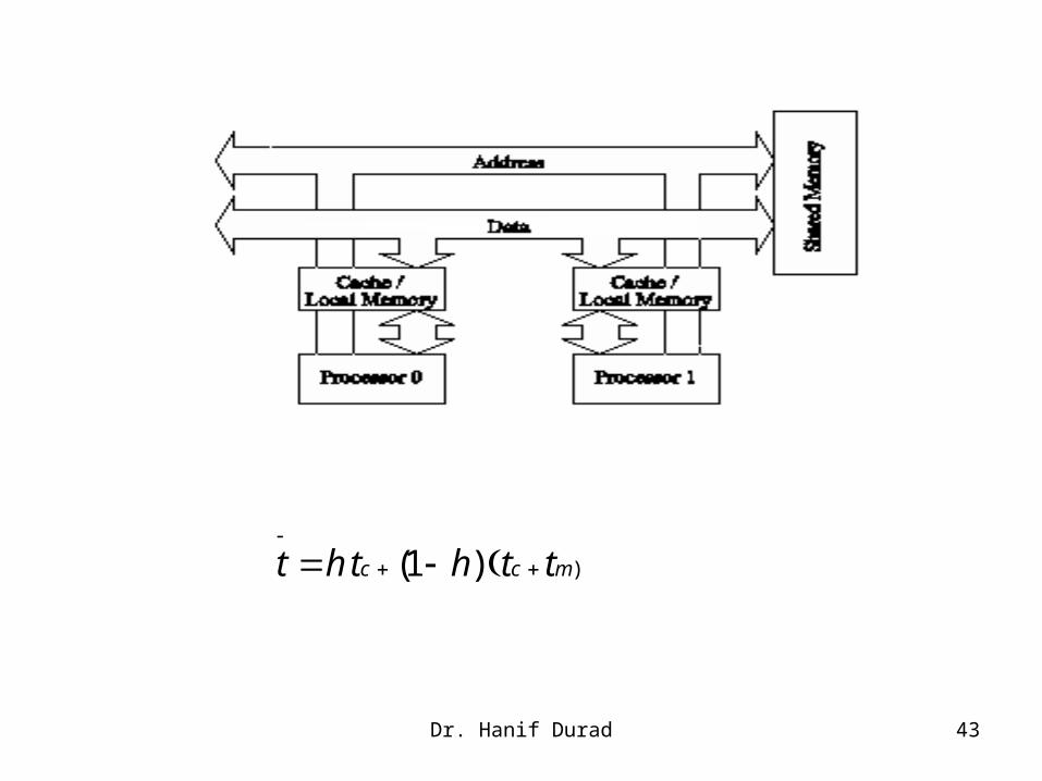
Consider the same setup as before, except in this case, the block size is 4 words instead of 1 word i.e., the processor can fetch a four-word cache line every 100 cycles. We repeat the dot-product computation in this scenario: Assuming that the vectors are laid out linearly in memory, eight
FLOPs (four multiply-adds) can be performed in 200 cycles. This is because a single memory access fetches four consecutive
words in the vector. Therefore, two accesses can fetch four elements of each of the
vectors. This corresponds to a FLOP every 25 ns, for a peak speed of 40 MFLOPS. (Exact? )
Impact of Memory Bandwidth: Example (2.4)
Dr. Hanif Durad 43
)(1 )c c mt h t h t t

Dr. Hanif Durad 44
Impact of Memory Bandwidth It is important to note that increasing block size does not
change latency of the system. Physically, the scenario illustrated here can be viewed as a
wide data bus (4 words or 128 bits) connected to multiple memory banks.
In practice, such wide buses are expensive to construct. In a more practical system, consecutive words are sent on
the memory bus on subsequent bus cycles after the first word is retrieved. (What change ?)

Dr. Hanif Durad 45
Impact of Memory Bandwidth
The above examples clearly illustrate how increased bandwidth results in higher peak computation rates.
The data layouts were assumed to be such that consecutive data words in memory were used by successive instructions (spatial locality of reference).
If we take a data-layout centric view, computations must be reordered to enhance spatial locality of reference.

Example 2.5 Impact of Strided Access
Consider the following code fragment:
for (i = 0; i < 1000; i++)
b[i] = 0.0;
for (j = 0; j < 1000; j++)
b[i] += A[j][i];
The code fragment sums columns of the matrix A into a vector b.
Dr. Hanif Durad 46

Dr. Hanif Durad 47
Multiplying a matrix with a vector: (a) multiplying column-by-column, keeping a running sum;
Small & fits cache

Dr. Hanif Durad 48
Impact of Memory Bandwidth: Example
The vector b is small and easily fits into the cache The matrix A is accessed in a column order. The strided access results in very poor performance.

Dr. Hanif Durad 49
Example 2.6 Eliminating Strided Access
We can fix the above code as follows:
for (i = 0; i < 1000; i++)
b[i] = 0.0;
for (j = 0; j < 1000; j++)
for (i = 0; i < 1000; i++)
b[i] += A[j][i];
In this case, the matrix is traversed in a row-order and performance can be expected to be significantly better.

Dr. Hanif Durad 50
Multiplying a matrix with a vector: (b) computing each element of the result as a dot product of a row of the
matrix with the vector.
The concept is called tiling or loop tiling

Dr. Hanif Durad 51
Memory System Performance: Summary
The series of examples presented in this section illustrate the following concepts: Exploiting spatial and temporal locality in applications is critical
for amortizing memory latency and increasing effective memory bandwidth.
The ratio of the number of operations to number of memory accesses is a good indicator of anticipated tolerance to memory bandwidth.
Memory layouts and organizing computation appropriately can make a significant impact on the spatial and temporal locality.

Dr. Hanif Durad 52
2.2.3 Alternate Approaches for Hiding Memory Latency
• Consider the problem of browsing the web on a very slow network connection. We deal with the problem in one of three possible ways: – we anticipate which pages we are going to browse ahead of
time and issue requests for them in advance; – we open multiple browsers and access different pages in each
browser, thus while we are waiting for one page to load, we could be reading others; or
– we access a whole bunch of pages in one go - amortizing the latency across various accesses.
• The first approach is called prefetching, the second multithreading, and the third one corresponds to spatial locality (already discussed) in accessing memory words.

2.2.3.1 Multithreading for Latency Hiding
A thread is a single stream of control in the flow of a program.
We illustrate threads with a simple example:
for (i = 0; i < n; i++) c[i] = dot_product(get_row(a, i), b);
Each dot-product is independent of the other, and therefore represents a concurrent unit of execution.
We can safely rewrite the above code segment as: for (i = 0; i < n; i++) c[i] = create_thread(dot_product,get_row(a, i),
b);
Example 2.7 Threaded execution of matrix multiplication

Dr. Hanif Durad 54
Multithreading for Latency Hiding: Example
In the code, the first instance of this function accesses a pair of vector elements and waits for them.
In the meantime, the second instance of this function can access two other vector elements in the next cycle, and so on.
After l units of time, where l is the latency of the memory system, the first function instance gets the requested data from memory and can perform the required computation.
In the next cycle, the data items for the next function instance arrive, and so on. In this way, in every clock cycle, we can perform a computation.

Dr. Hanif Durad 55
Multithreading for Latency Hiding
The execution schedule in the previous example is predicated upon two assumptions: the memory system is capable of servicing multiple outstanding requests, and the processor is capable of switching threads at every cycle.
It also requires the program to have an explicit specification of concurrency in the form of threads.
Machines such as the HEP and Tera rely on multithreaded processors that can switch the context of execution in every cycle. Consequently, they are able to hide latency effectively.

56
2.2.3.2 Prefetching for Latency Hiding
Misses on loads cause programs to stall. Why not advance the loads so that by the time
the data is actually needed, it is already there! The only drawback is that you might need more
space to store advanced loads. However, if the advanced loads are overwritten,
we are no worse than before! Hiding latency by prefetching Example 2.8
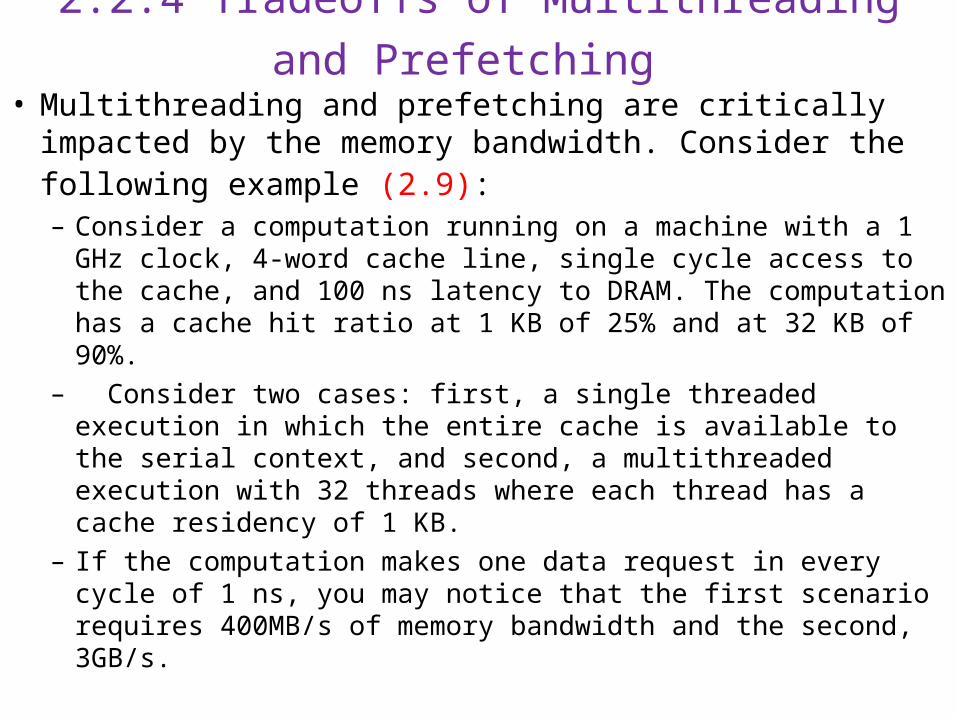
2.2.4 Tradeoffs of Multithreading and Prefetching • Multithreading and prefetching are critically impacted
by the memory bandwidth. Consider the following example (2.9): – Consider a computation running on a machine with a 1 GHz
clock, 4-word cache line, single cycle access to the cache, and 100 ns latency to DRAM. The computation has a cache hit ratio at 1 KB of 25% and at 32 KB of 90%.
– Consider two cases: first, a single threaded execution in which the entire cache is available to the serial context, and second, a multithreaded execution with 32 threads where each thread has a cache residency of 1 KB.
– If the computation makes one data request in every cycle of 1 ns, you may notice that the first scenario requires 400MB/s of memory bandwidth and the second, 3GB/s.

Tradeoffs of Multithreading and Prefetching
• Bandwidth requirements of a multithreaded system may increase very significantly because of the smaller cache residency of each thread.
• Multithreaded systems become bandwidth bound instead of latency bound.
• Multithreading and prefetching only address the latency problem and may often exacerbate the bandwidth problem.
• Multithreading and prefetching also require significantly more hardware resources in the form of storage.

Dr. Hanif Durad 59
Explicitly Parallel Platforms

Dr. Hanif Durad 60
2.3 Dichotomy of Parallel Computing Platforms
An explicitly parallel program must specify concurrency and interaction between concurrent subtasks.
The former is sometimes also referred to as the control structure and the latter as the communication model.

Example 2.10 Parallelism from single instruction on multiple processors
Consider the following code segment that adds two vectors:
for (i = 0; i < 1000; i++) c[i] = a[i] + b[i]; various iterations of the loop are independent
of each other; can all be executed independently on all the processors with appropriate data
we could execute this loop much fasterDr. Hanif Durad 61

Dr. Hanif Durad 62
2.3.1 Control Structure of Parallel Programs
Parallelism can be expressed at various levels of granularity - from instruction level to processes.
Between these extremes exist a range of models, along with corresponding architectural support.
Best explained by Flynn’s Taxonomy of Computer Architecture

Dr. Hanif Durad 63
Flynn’s Taxonomy of ComputerArchitecture
Processing units in parallel computers either operate under the centralized control of a single control unit or work independently.
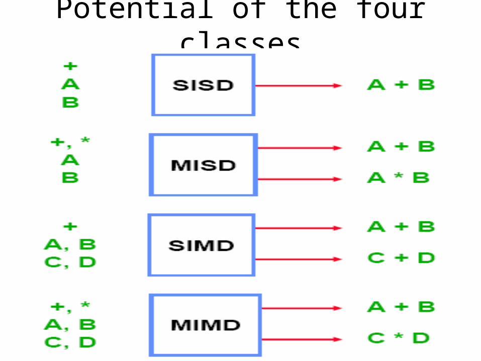
Single Instruction Single Data (SISD) Single Instruction Multiple Data (SIMD) Multiple Instruction Multiple Data (MIMD) Multiple Instruction Single Data (MISD)
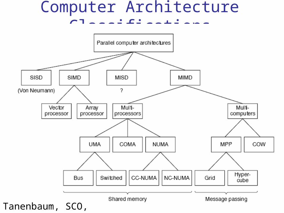
Computer Architecture Classifications
Tanenbaum, SCO, P-104
Dr. Hanif Durad 65
Potential of the four classes

Dr. Hanif Durad 66
2.3.1.1 SISD Architecture
A single-processor computer (uniprocessor) in which a single stream of instructions is generated from the program.
Hesham, P-5

Dr. Hanif Durad 67
2.3.1.2 SIMD Architecture
Each instruction is executed on a different set of data by different processors. (Used for vector and array processing)

SIMD Architecture
Dr. Hanif Durad 68

Dr. Hanif Durad 69
2.3.1.3 MIMD Architecture
If each processor has its own control control unit, each processor can execute different instructions on different data items. This model is called multiple instruction stream, multiple data stream (MIMD).

Dr. Hanif Durad 70
SIMD and MIMD Architectures
A typical SIMD architecture (a) and a typical MIMD architecture (b).

Dr. Hanif Durad 71
SIMD Processors
Some of the earliest parallel computers such as the Illiac IV, MPP, DAP, CM-2, and MasPar MP-1 belonged to this class of machines.
Variants of this concept have found use in co-processing units such as the MMX units in Intel processors and DSP chips such as the Sharc.

Dr. Hanif Durad 72
SIMD Processors
SIMD relies on the regular structure of computations (such as those in image processing).
It is often necessary to selectively turn off operations on certain data items. For this reason, most SIMD programming paradigms allow for an ``activity mask'', which determines if a processor should participate in a computation or not.

Dr. Hanif Durad 73
Example 2.11 Execution of conditional statements on a SIMD architecture
If (B==0)
C=A;
Else
C=A/B;
Executing a conditional statement on an SIMD computer with four processors: (a) the conditional statement;.
(a)

Dr. Hanif Durad 74
Conditional Execution in SIMD Processors
(b) the execution of the statement in two steps.

Dr. Hanif Durad 75
MIMD Processors
In contrast to SIMD processors, MIMD processors can execute different programs on different processors.
A variant of this, called single program multiple data streams (SPMD) executes the same program on different processors.
Dr. Hanif Durad 76
MIMD Processors
It is easy to see that SPMD and MIMD are closely related in terms of programming flexibility and underlying architectural support.
Examples of such platforms include current generation Sun Ultra Servers, SGI Origin Servers, multiprocessor PCs, workstation clusters, and the IBM SP.

Dr. Hanif Durad 77
SIMD-MIMD Comparison SIMD computers require less hardware than MIMD
computers (single control unit). However, since SIMD processors ae specially designed,
they tend to be expensive and have long design cycles. Not all applications are naturally suited to SIMD
processors. In contrast, platforms supporting the SPMD paradigm can
be built from inexpensive off-the-shelf components with relatively little effort in a short amount of time.

Dr. Hanif Durad 78
2.3.1.3 Multiple Instruction Single Data (MISD)
• Multiple PEs operate on different Instructions but use same data• Never been commercially implemented • More of an intellectual exercise than a practical configuration• Some people say systolic arrays
Data InputStream
Data OutputStream
Processor
A
Processor
B
Processor
C
InstructionStream A
InstructionStream B
Instruction Stream C
With thanks to Rajkumar BuyyaFile: ParallelCompOverview.ppt

Dr. Hanif Durad 79
2.3.2 Communication Model of Parallel Platforms
There are two primary forms of data exchange between parallel tasks - accessing a shared data space and exchanging messages.
Platforms that provide a shared data space are called shared-address-space machines or multiprocessors.
Platforms that support messaging are also called message passing platforms or multicomputers.

Computer Architecture Classifications
Tanenbaum, SCO, P-104
(SMP) (SMP)
threads (POSIX, NT) and directives (OpenMP) MPI and PVM

Dr. Hanif Durad 81
2.3.2 .1 Shared-Address-Space Platforms
Part (or all) of the memory is accessible to all processors. Processors interact by modifying data objects stored in this
shared-address-space. If the time taken by a processor to access any memory
word in the system global or local is identical, the platform is classified as a uniform memory access (UMA), else, a non-uniform memory access (NUMA) machine.

Dr. Hanif Durad 82
NUMA and UMA Shared-Address-Space Platforms
Typical shared-address-space architectures: (a) Uniform-memory access shared-address-space computer; (b) Uniform-memory-access shared-address-space computer with caches and memories; (c) Non-uniform-memory-access shared-address-space computer with local memory only.

NUMA and UMA The distinction between NUMA and UMA platforms
is important from the point of view of algorithm design.
NUMA machines require locality from underlying algorithms for performance.
Programming these platforms is easier since reads and writes are implicitly visible to other processors.
However, read-write data to shared data must be coordinated (this will be discussed in greater detail when we talk about threads programming) Caches in such machines require coordinated access to multiple copies. This leads to the cache coherence problem.

Dr. Hanif Durad 84
NUMA and UMA Shared-Address-Space Platforms
Caches in such machines require coordinated access to multiple copies. This leads to the cache coherence problem.
A weaker model of these machines provides an address map, but not coordinated access. These models are called non cache coherent shared address space machines.

Shared-Address-Space Platforms
Shared-address-space programming paradigms such as threads (POSIX, NT) and directives (OpenMP) therefore support synchronization using locks and related mechanisms.
Dr. Hanif Durad 85
Dr. Hanif Durad 86
Shared-Address-Space vs. Shared Memory Machines
It is important to note the difference between the terms shared address space and shared memory.
We refer to the former as a programming abstraction and to the latter as a physical machine attribute.
It is possible to provide a shared address space using a physically distributed memory.

Dr. Hanif Durad 87
2.3.2 .2 Message-Passing Platforms
These platforms comprise of a set of processors and their own (exclusive) memory.
Instances of such a view come naturally from clustered workstations and non-shared-address-space multicomputers.
These platforms are programmed using (variants of) send and receive primitives.
Libraries such as MPI and PVM provide such primitives.

Dr. Hanif Durad 88
Message Passing vs. Shared Address Space Platforms
Message passing requires little hardware support, other than a network.
Shared address space platforms can easily emulate message passing. The reverse is more difficult to do (in an efficient manner).

Dr. Hanif Durad 89
Wilkinson, P-15 Wilkinson, P-27

Dr. Hanif Durad 90
2.4 Physical Organization of Parallel Platforms
We begin this discussion with an ideal parallel machine called Parallel Random Access Machine, or PRAM.

Dr. Hanif Durad 91
2.4.1 Architecture of an Ideal Parallel Computer
A natural extension of the Random Access Machine (RAM) serial architecture is the Parallel Random Access Machine, or PRAM.
PRAMs consist of p processors and a global memory of unbounded size that is uniformly accessible to all processors.
Processors share a common clock but may execute different instructions in each cycle.

Dr. Hanif Durad 92
Architecture of an Ideal Parallel Computer
Depending on how simultaneous memory accesses are handled, PRAMs can be divided into four subclasses. Exclusive-read, exclusive-write (EREW) PRAM. Concurrent-read, exclusive-write (CREW) PRAM. Exclusive-read, concurrent-write (ERCW) PRAM. Concurrent-read, concurrent-write (CRCW) PRAM.
Dr. Hanif Durad 93
Architecture of an Ideal Parallel Computer
What does concurrent write mean, anyway? Common: write only if all values are identical. Arbitrary: write the data from a randomly selected
processor. Priority: follow a predetermined priority order. Sum: Write the sum of all data items. (?)

Dr. Hanif Durad 94
2.4.1.1 Architectural Complexity of an Ideal Parallel Computer
Processors and memories are connected via switches.
Since these switches must operate in O(1) time at the level of words, for a system of p processors and m words, the switch complexity is O(mp).
Clearly, for meaningful values of p and m, a true PRAM is not realizable.

Dr. Hanif Durad 95
2.4.2 Interconnection Networks for Parallel Computers
Interconnection networks carry data between processors and to memory.
Interconnects are made of switches and links (wires, fiber).
Interconnects are classified as static or dynamic.

Dr. Hanif Durad 96
Interconnection Networks for Parallel Computers
Static networks consist of point-to-point communication links among processing nodes and are also referred to as direct networks.
Dynamic networks are built using switches and communication links. Dynamic networks are also referred to as indirect networks.

Dr. Hanif Durad 97
Static and Dynamic Interconnection Networks
Classification of interconnection networks: (a) a static network; and (b) a dynamic network.

Dr. Hanif Durad 98
Interconnection Networks
Switches map a fixed number of inputs to outputs.
The total number of ports on a switch is the degree of the switch.
The cost of a switch grows as the square of the degree of the switch, the peripheral hardware linearly as the degree, and the packaging costs linearly as the number of pins.
Dr. Hanif Durad 99
Interconnection Networks: Network Interfaces
Processors talk to the network via a network interface.
The network interface may hang off the I/O bus or the memory bus.
In a physical sense, this distinguishes a cluster from a tightly coupled multicomputer.
The relative speeds of the I/O and memory buses impact the performance of the network.

Dr. Hanif Durad 100
2.4.3 Network Topologies
A variety of network topologies have been proposed and implemented.
These topologies tradeoff performance for cost. Commercial machines often implement hybrids
of multiple topologies for reasons of packaging, cost, and available components.
Dr. Hanif Durad 101
2.4.3.1 Network Topologies: Buses
Some of the simplest and earliest parallel machines used buses.
All processors access a common bus for exchanging data.
The distance between any two nodes is O(1) in a bus. The bus also provides a convenient broadcast media.

Dr. Hanif Durad 102
Network Topologies: Buses
However, the bandwidth of the shared bus is a major bottleneck.
Typical bus based machines are limited to dozens of nodes.
Sun Enterprise servers and Intel Pentium based shared-bus multiprocessors are examples of such architectures.
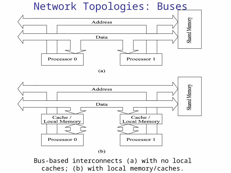
Network Topologies: Buses
Bus-based interconnects (a) with no local caches; (b) with local memory/caches.
Dr. Hanif Durad 104
Network Topologies: Buses
Since much of the data accessed by processors is local to the processor, a local memory can improve the performance of bus-based machines.
Dr. Hanif Durad 105
2.4.3.2 Network Topologies: Crossbars
A crossbar network uses an p×m grid of switches to connect p inputs to m outputs in a non-blocking manner

Dr. Hanif Durad 106
Figure 8.17 Crossbar switch with three inputs and four outputs
FOROUZAN, P-228

Dr. Hanif Durad 107
Network Topologies: Crossbars
A completely non-blocking crossbar network connecting p processors to b memory banks.

Dr. Hanif Durad 108
Network Topologies: Crossbars
The cost of a crossbar of p processors grows as O(p2).
This is generally difficult to scale for large values of p.
Examples of machines that employ crossbars include the Sun Ultra HPC 10000 and the Fujitsu VPP500.

Dr. Hanif Durad 109
2.4.3.3 Network Topologies: Multistage Networks
Crossbars have excellent performance scalability but poor cost scalability.
Buses have excellent cost scalability, but poor performance scalability.
An intermediate class of networks called multistage interconnection networks (MINs) strike a compromise between these extremes

Dr. Hanif Durad 110
Network Topologies: Multistage Networks
The schematic of a typical multistage interconnection network.

Dr. Hanif Durad 111
Network Topologies: Multistage Omega Network
One of the most commonly used multistage interconnects is the Omega network.
This network consists of log p stages, where p is the number of inputs/outputs.
At each stage, input i is connected to output j if:

Dr. Hanif Durad 112
Network Topologies: Multistage Omega Network
Each stage of the Omega network implements a perfect shuffle as follows:
A perfect shuffle interconnection for eight inputs and outputs.

Dr. Hanif Durad 113
Network Topologies: Multistage Omega Network
The perfect shuffle patterns are connected using 2×2 switches.
The switches operate in two modes – crossover or passthrough.
Two switching configurations of the 2 × 2 switch: (a) Pass-through; (b) Cross-over.
Dr. Hanif Durad 114
A complete Omega network with the perfect shuffle interconnects and switches can now be illustrated:
Network Topologies: Multistage Omega Network

Network Topologies: Multistage Omega Network
•A complete omega network connecting eight inputs and eight outputs.•An omega network has p/2 × log p switching nodes, and the cost of such a network grows as (p log p). Here p=8
p/2 × log p=4x3=12p log p=8x3=24

Dr. Hanif Durad 116
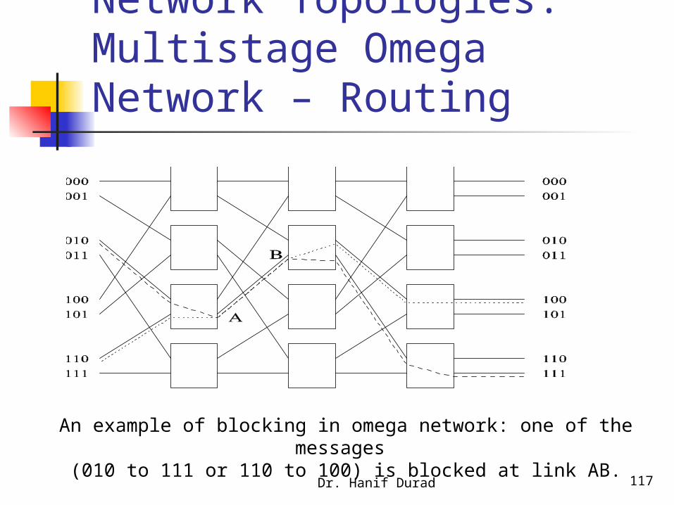
Network Topologies:Multistage Omega Network – Routing
Let s be the binary representation of the source and d be that of the destination processor.
The data traverses the link to the first switching node. If the most significant bits of s and d are the same, then the data is routed in pass-through mode by the switch else, it switches to crossover.
This process is repeated for each of the log p switching stages.
Note that this is not a non-blocking switch.
Dr. Hanif Durad 117
Network Topologies: Multistage Omega Network – Routing
An example of blocking in omega network: one of the messages (010 to 111 or 110 to 100) is blocked at link AB.

Dr. Hanif Durad 118
Figure 8.18 Multistage switchFOROUZAN, P-228

Dr. Hanif Durad 119
In a three-stage switch, the total number of cross-points is
2kN + k(N/n)2
which is much smaller than the number of cross-points in a single-stage switch
(N2).
FOROUZAN, P-229

Dr. Hanif Durad 120
Design a three-stage, 200 × 200 switch (N = 200) with k = 4 and n = 20.
SolutionIn the first stage we have N/n or 10 crossbars, each of size 20 × 4. In the second stage, we have 4 crossbars, each of size 10 × 10. In the third stage, we have 10 crossbars, each of size 4 × 20. The total number of crosspoints is 2kN + k(N/n)2, or 2000 crosspoints. This is 5 percent of the number of crosspoints in a single-stage switch (200 × 200 = 40,000).
Example 8.3
FOROUZAN, P-229

Dr. Hanif Durad 121
2.4.3.4 Completely Connected Network
Each processor is connected to every other processor. The number of links in the network scales as O(p2). While the performance scales very well, the hardware
complexity is not realizable for large values of p. In this sense, these networks are static counterparts of
crossbars. # of interconnections=?

Dr. Hanif Durad 122
Completely Connected Networks
Example of an 8-node completely connected network.
(a) A completely-connected network of eight nodes;

Dr. Hanif Durad 123
2.4.3.5 Star Connected Network
Every node is connected only to a common node at the center.
Distance between any pair of nodes is O(1). However, the central node becomes a bottleneck
In this sense, star connected networks are static counterparts of buses.

Dr. Hanif Durad 124
Star Connected Networks
Example of an 8-node star connected network.
(b) a star connected network of nine nodes.

Dr. Hanif Durad 125
2.4.3.6 Linear Arrays, Meshes, and k-d Meshes
Due to the large number of links in completely connected networks, sparser networks are typically used to build parallel computers
A family of such networks spans the space of linear arrays and hypercubes

Dr. Hanif Durad 126
2.4.3.6.1 Linear Arrays
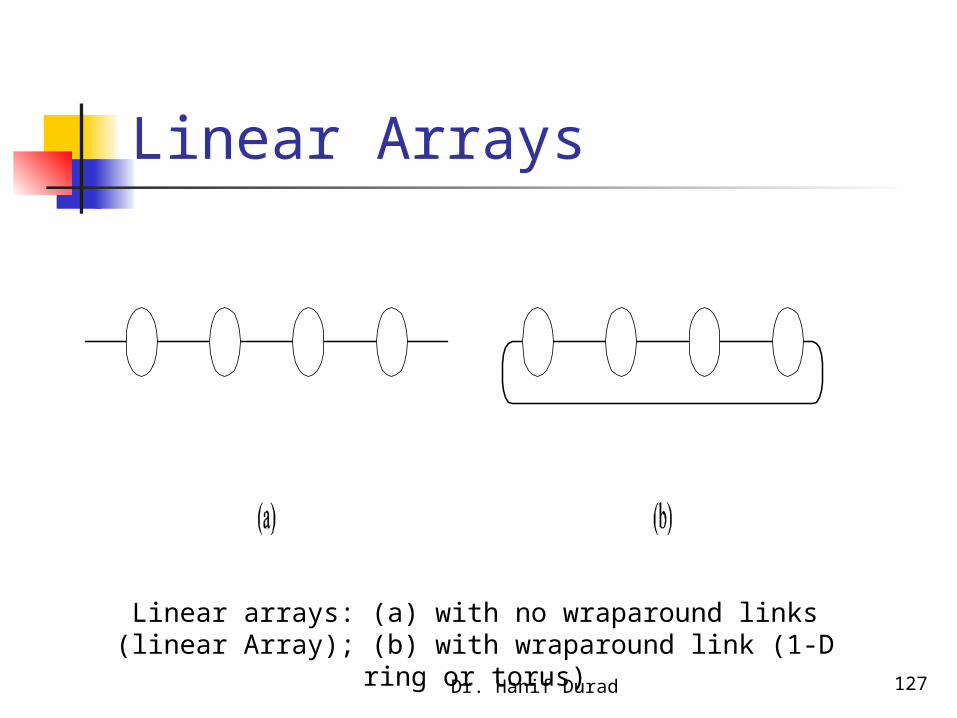
In a linear array, each node has two neighbors, one to its left and one to its right. If the nodes at either end are connected, we refer to it as a 1-D torus or a ring.
Dr. Hanif Durad 127
Linear Arrays
Linear arrays: (a) with no wraparound links (linear Array); (b) with wraparound link (1-D ring or torus)
Dr. Hanif Durad 128
2.4.3.6.2 Meshes, and k-d Meshes
A generalization to 2 dimensions has nodes with 4 neighbors, to the north, south, east, and west.
A further generalization to d dimensions has nodes with 2d neighbors.

Dr. Hanif Durad 129
Two- and Three Dimensional Meshes
Two and three dimensional meshes: (a) 2-D mesh with no wraparound; (b) 2-D mesh with wraparound link (2-D torus); and
(c) a 3-D mesh with no wraparound.

Dr. Hanif Durad 130
2.4.3.6.3 Hypercubes

Properties of Hypercubes
A special case of a d-dimensional mesh is a hypercube. Here, d = log p, where p is the total number of nodes
The distance between any two nodes is at most log p Each node has log p neighbors. The distance between two nodes is given by the
number of bit positions at which the two nodes differ (XOR)

Dr. Hanif Durad 132
Hypercubes and their Construction

Dr. Hanif Durad 133
2.4.3.6.4 Tree-Based Networks
Complete binary tree networks: (a) a static tree network; and (b) a dynamic tree network.
Dr. Hanif Durad 134
Tree Properties
The distance between any two nodes is no more than 2logp
Links higher up the tree potentially carry more traffic than those at the lower levels.
For this reason, a variant called a fat-tree, fattens the links as we go up the tree.
Trees can be laid out in 2D with no wire crossings. This is an attractive property of trees.

Dr. Hanif Durad 135
Fat Trees
A fat tree network of 16 processing nodes.

Dr. Hanif Durad 136
2.4.4 Evaluating Static Interconnection Networks
Various criteria used to characterize the cost and performance of static interconnection include Diameter Bisection Width Cost

Dr. Hanif Durad 137
2.4.4.1 Diameter
Diameter: The distance between the farthest two nodes in the network.
The diameter of linear array is p − 1, mesh is 2( − 1), tree and hypercube is log p, completely connected network is O(1).
Dr. Hanif Durad 138
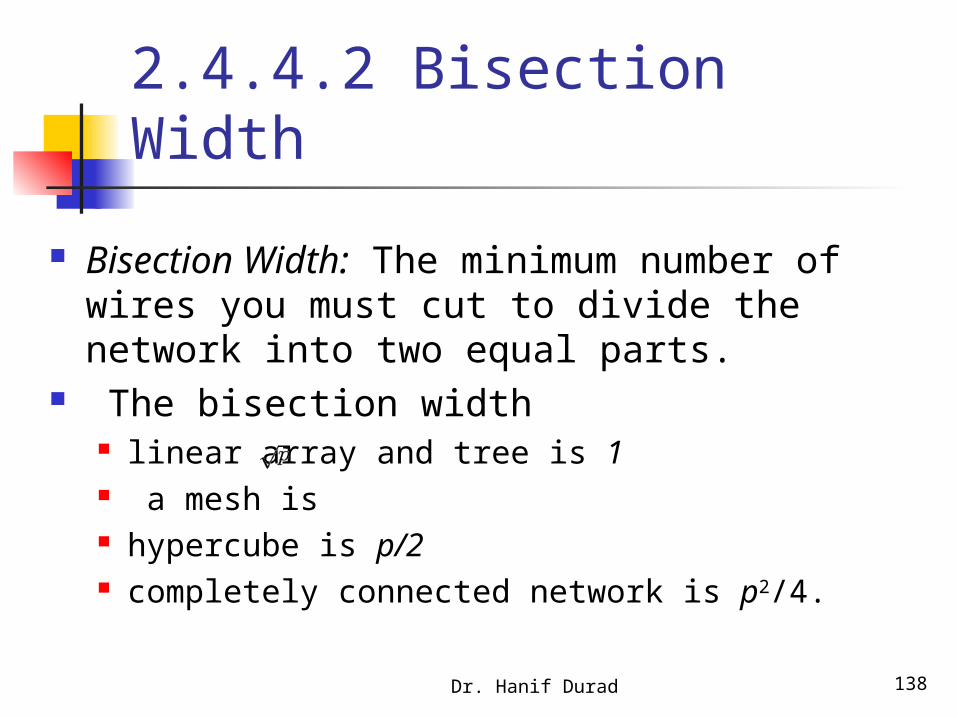
2.4.4.2 Bisection Width
Bisection Width: The minimum number of wires you must cut to divide the network into two equal parts.
The bisection width linear array and tree is 1 a mesh is hypercube is p/2 completely connected network is p2/4.

Dr. Hanif Durad 139
2.4.4.2 Cost
The number of links or switches (whichever is asymptotically higher) is a meaningful measure of the cost.
However, a number of other factors, such as the ability to layout the network, the length of wires, etc., also factor in to the cost.

140
Evaluating Static Interconnection Networks
Network Diameter BisectionWidth
Arc Connecti-vity
Cost (No. of links)
Completely-connected
Star
Complete binary tree
Linear array
2-D mesh, no wraparound
2-D wraparound mesh
Hypercube
Wraparound k-ary d-cube
Not Discussed

Dr. Hanif Durad 141
2.4.5 Evaluating Dynamic Interconnection Networks
Network Diameter Bisection Width
Arc Connectivity
Cost (No. of links)
Crossbar
Omega Network
Dynamic Tree
Self Study
*This measure appears off..
Our 3 stage, 8 in/out network has 32 links or p*(log(p) + 1) links
2.4.6 Cache Coherence in Multiprocessor Systems
One or two levels of cache typically associated with each processor – this is essential for performance
Problem Multiple copies of same data in different caches Can result in an inconsistent view of memory

Write Policy Review Write back policy
Write goes only to cache Main memory updated only when cache block is
replaced Can lead to inconsistency
Write through policy All writes made to cache and main memory Inconsistencies can occur unless all caches monitor
memory traffic

Dr. Hanif Durad 144
Basic Cache Coherency Methods
Cache-memory coherence using two policies:
Hesham, Chapter 04, P-8/61

Software Solutions
Compiler and operating system deal with problem Overhead transferred to compile time Design complexity transferred from hardware to
software Software tends to make conservative decisions
leading to inefficient cache utilization Analyze code to determine safe periods for
caching shared variables WSCOA7e, P-650
Hardware Solution
Cache coherence protocols Dynamic recognition of potential problems Run time More efficient use of cache Transparent to programmer Snoopy protocols Directory protocols

Dr. Hanif Durad 147
Snoopy Protocols-Cache Coherence in Multiprocessor
Systems
Cache coherence in multiprocessor systems: (a) Invalidate protocol;
When the value of a variable is changes, all its copies must either be invalidated or updated.

Dr. Hanif Durad 148
Cache Coherence in Multiprocessor Systems
Cache coherence in multiprocessor systems: (b) Update protocol for shared variables.

Dr. Hanif Durad 149
Cache Coherence: Update and Invalidate Protocols
• If a processor just reads a value once and does not need it again, an update protocol may generate significant overhead
• If two processors make interleaved test and updates to a variable, an update protocol is better.
• Both protocols suffer from false sharing overheads (two words that are not shared, however, they lie on the same cache line).
• Most current machines use invalidate protocols
Dr. Hanif Durad 150
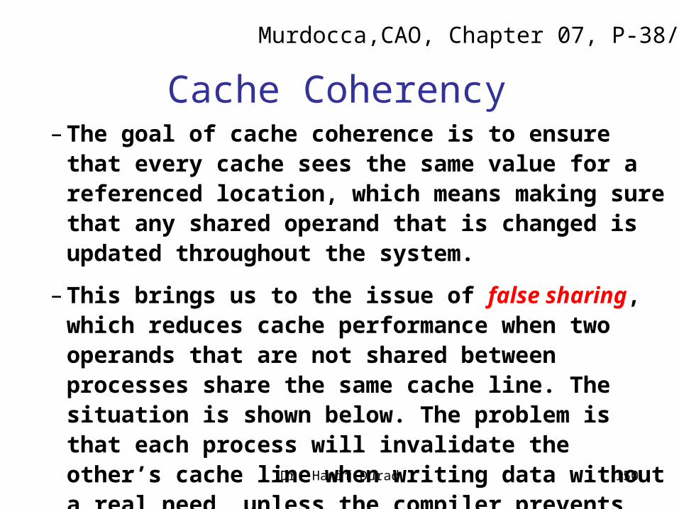
Cache Coherency– The goal of cache coherence is to ensure that every cache sees
the same value for a referenced location, which means making sure that any shared operand that is changed is updated throughout the system.
– This brings us to the issue of false sharing, which reduces cache performance when two operands that are not shared between processes share the same cache line. The situation is shown below. The problem is that each process will invalidate the other’s cache line when writing data without a real need, unless the compiler prevents this.
Murdocca,CAO, Chapter 07, P-38/53

Dr. Hanif Durad 151
Cache Coherency
Murdocca, CAO, Chapter 07, P-38/53

Dr. Hanif Durad 152
2.4.6.1 Maintaining Coherence Using Invalidate Protocols
• Each copy of a data item is associated with a state.
• One example of such a set of states is shared, invalid, or dirty.
• In shared state, the line in the shared by many processors
• In dirty/modified state, only one copy exists and therefore, no invalidates need to be generated.
• In invalid state, the data copy is invalid, therefore, a read generates a data request (and associated state changes).

Cache line has 4 states
Each line of a cache has associated with it two bits – four states
Modified – line in this cache is modified and only valid in this cache
Exclusive – line in this cache is same as that in memory (unmodified) and not present in any other cache
Shared – line in this cache is same as that in memory (unmodified) and may also be present in another cache
Invalid – line in this cache contains bad data
MESI-ProtocolUsed in Intel
MSI-Protocol MOESI-ProtocolUsed in AMDHB PC & Stat. , P-51

Dr. Hanif Durad 154
Maintaining Coherence Using Invalidate Protocols
State diagram of a simple three-state coherence protocol.
MSI-Protocol

Dr. Hanif Durad 155
Maintaining Coherence Using Invalidate Protocols
Example of parallel program execution with the simple
three-state coherence protocol.
D=Modified /DirtyS=SharedI=Invalid

Write Invalidate (a.k.a. MESI) Multiple readers, one writer When a write is required, command is issued and
all other caches of the line are invalidated Writing processor then has exclusive (cheap)
access until line required by another processor A state is associated with every line
Modified Exclusive Shared Invalid

Write Update (a.k.a. write broadcast)
Multiple readers and writers Updated word is distributed to all other
processors

Snoopy Protocols –Implementations Performance of these two implementations
depends on number of caches and pattern of read/writes
Some systems use adaptive protocols to use both methods
Write invalidate most common – Used in Pentium 4 and PowerPC systems

MESI Protocol Each line of a cache has associated with it two bits –
four states Modified – line in this cache is modified and only valid
in this cache Exclusive – line in this cache is same as that in memory
(unmodified) and not present in any other cache Shared – line in this cache is same as that in memory
(unmodified) and may also be present in another cache Invalid – line in this cache contains bad data Write throughs from an L1 cache to an L2 cache makes
it visible to the MESI protocol

MESI Protocol (continued)

MESI – State Transition Diagram

Dr. Hanif Durad 162
Snoopy Cache Systems•How are invalidates sent to the right processors?•In snoopy caches, there is a broadcast media that listens to all invalidates and read requests and performs appropriate coherence operations locally.
A simple snoopy bus based cache coherence system.

Performance of Snoopy Caches
Once copies of data are tagged dirty, all subsequent operations can be performed locally on the cache without generating external traffic.
If a data item is read by a number of processors, it transitions to the shared state in the cache and all subsequent read operations become local.
If processors read and update data at the same time, they generate coherence requests on the bus - which is ultimately bandwidth limited.
Dr. Hanif Durad 163

2.4.6.2 Directory Based Systems
In snoopy caches, each coherence operation is sent to all processors. This is an inherent limitation.
Why not send coherence requests to only those processors that need to be notified?
This is done using a directory, which maintains a presence vector for each data item (cache line) along with its global state
Dr. Hanif Durad 164

Directory Protocols – Central control
Central memory controller maintains directory of: where blocks are held in which caches they are held what state the data is in
Appropriate transfers are performed by controller

Directory Protocols – Write Process
Requests to write to a line are made to controller Using directory, controller tells all other processors
with copy of same data to invalidate Write is granted to requesting processor and that
processor has exclusive rights to that data Request to read from another processor forces
controller to issue command to processor with exclusive rights to update (write back) main memory.

Directory Protocols (continued)
Problems Creates central bottleneck Communication overhead
Effective in large scale systems with complex interconnection schemes

Dr. Hanif Durad 168
Directory Based Systems
Architecture of typical directory based systems: (a) a centralized directory; and (b) a distributed directory.

Performance of Directory Based Schemes
The need for a broadcast media is replaced by the directory.
The additional bits to store the directory may add significant overhead.
The underlying network must be able to carry all the coherence requests.
The directory is a point of contention, therefore, distributed directory schemes must be used.
Dr. Hanif Durad 169

2.5 Communication Costs in Parallel Machines (1/2)
Major overheads in the execution of parallel programs: from communication of information between processing elements.
The cost of communication is dependent on a variety of features including: programming model semantics, network topology, data handling and routing, and associated software protocols.
170
Communication Costs in Parallel Machines (2/2)
Time taken to communicate a message between two nodes in a network = time to prepare a message for transmission + time taken by the message to traverse the network to its destination.
Dr. Hanif Durad 171

2.5.1 Message Passing Costs in Parallel Computers (1/3)
Startup time (ts): The startup time is the time required to handle a message at the sending and receiving nodes.
Includes the time to prepare the message (adding header, trailer & error
correction information), the time to execute the routing algorithm, and the time to establish an interface between the local node and the
router. This delay is incurred only once for a single message
transfer.Dr. Hanif Durad 172

Message Passing Costs in Parallel Computers (2/3)
Per-hop time (th): After a message leaves a node, it takes a finite amount
of time to reach the next node in its path. The time taken by the header of a message to travel
between two directly connected nodes in the network It is also known as node latency Is directly related to the latency within the routing
switch for determining which output buffer or channel the message should be forwarded to.
Dr. Hanif Durad 173

2.5.1 Message Passing Costs in Parallel Computers (3/3)
Per-word transfer time (tw): If the channel bandwidth is r words per second, then
each word takes time tw = 1/r to traverse the link. This time includes network as well as buffering
overheads..
Dr. Hanif Durad 174

Terminalogy
transmission time time taken to emit all bits into medium
propagation time time for a bit to traverse the link
Dr. Hanif Durad 175
Latency=propagation time+ transmission time+ queing time+ processing delay
FOROUZAN DCN , P-90
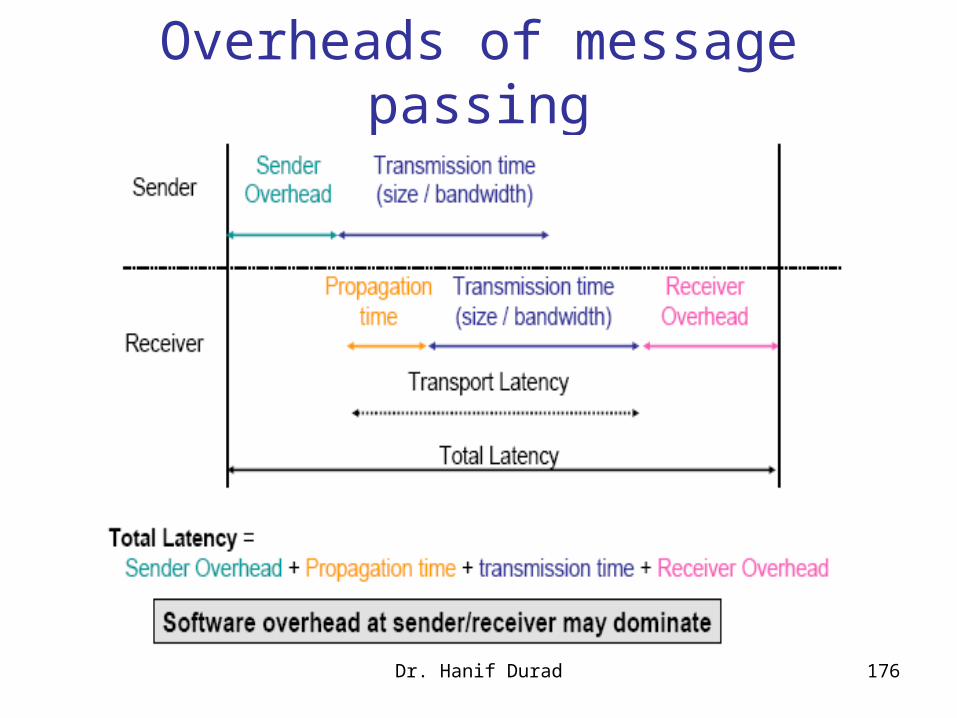
Overheads of message passing
Dr. Hanif Durad 176

2.5.1.1 Store-and-Forward Routing
When a message is traversing a path with multiple links, each intermediate node on the path forwards the message to the next node after it has received and stored the entire message.
Suppose that a message of size m is being transmitted through such a network. Assume that it traverses l links.
At each link, the message incurs a cost th for the header and twm for the rest of the message to traverse the link.
Dr. Hanif Durad 177

Store-and-Forward Routing
Since there are l such links, the total time is (th + twm)l.
Therefore, for store-and-forward routing, the total communication cost for a message of size m words to traverse l communication links is
Dr. Hanif Durad 178

Store-and-Forward Routing
In current parallel computers, the per-hop time th is quite small.
For most parallel algorithms, it is less than twm even for small values of m and thus can be ignored.
For parallel platforms using store-and-forward routing, the time given by the above equation can be simplified to
Dr. Hanif Durad 179

Dr. Hanif Durad 180
Store-and-Forward Routing
The environment of the network layer protocols.
Tanenbaum, Chapter 05, Fig 5-1

Dr. Hanif Durad 181
Store-and-Forward Routing
Passing a message from node P0 to P3 (a) through a store-and-forward communication network;

2.5.1.2 Packet Routing (1/8)
Store-and-forward: message is sent from one node to the next only after the entire message has been received
Consider the scenario in which the original message is broken into two equal sized parts before it is sent. An intermediate node waits for only half of the
original message to arrive before passing it on.
Dr. Hanif Durad 182

Packet Routing (2/8)
A step further: breaks the message into four parts.
In addition to better utilization of communication resources, this principle offers other advantages: lower overhead from packet loss (errors), possibility of packets taking different paths, and better error correction capability.
Dr. Hanif Durad 183

Packet Routing (3/8)
This technique is the basis for long-haul communication networks such as the Internet, where error rates, number of hops, and variation in network state can be higher.
The overhead here is that each packet must carry routing, error correction, and sequencing information.
Dr. Hanif Durad 184

Dr. Hanif Durad 185
Packet Routing (4/8)
Passing a message from node P0 to P3 (b) and (c) extending the concept to cut-through routing. The shaded regions represent the time that the message is in transit. The startup time associated with this message transfer is assumed to be zero.

Dr. Hanif Durad 186
Packet Routing (5/8)
Passing a message from node P0 to P3 (b) and (c) extending the concept to cut-through routing. The shaded regions represent the time that the message is in transit. The startup time associated with this message transfer is assumed to be zero.

Packet Routing (6/8)
Consider the transfer of an m word message through the network.
Assume: routing tables are static over the time of message transfer - all
packets traverse the same path The time taken for programming the network interfaces &
computing the routing info, is independent of the message length and is aggregated into the startup time ts
Size of a packet: r + s, r = original message, s = additional information carried in the packet
187

Packet Routing (7/8)
Time for packetizing the message is proportional to the length of the message: mtw1.
The network is capable of communicating one word every tw2 seconds,
Incurs a delay of th on each hop, and The first packet traverses l hops,
Then the packet takes time thl + tw2(r + s) to reach the destination.
Dr. Hanif Durad 188
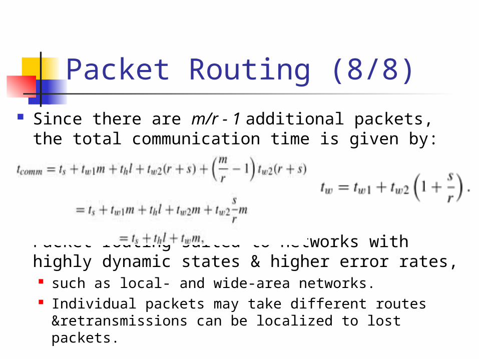
Packet Routing (8/8)
Since there are m/r - 1 additional packets, the total communication time is given by:
Packet routing suited to networks with highly dynamic states & higher error rates, such as local- and wide-area networks. Individual packets may take different routes &retransmissions
can be localized to lost packets.

General Observation (1/2)
In interconnection networks for parallel computers, additional restrictions can be imposed on message transfers to further reduce the overheads associated with packet switching
By forcing all packets to take the same path, we can eliminate the overhead of transmitting routing information with each packet.
By forcing in-sequence delivery, sequencing information can be eliminated.
Dr. Hanif Durad 190

General Observation (2/2)
By associating error information at message level rather than packet level, the overhead associated with error detection and correction can be reduced.
Finally, since error rates in interconnection networks for parallel machines are extremely low, lean error detection mechanisms can be used instead of expensive error correction schemes.
Routing scheme resulting from these optimizations: cut-through routing.

Dr. Hanif Durad 192
2.5.1.3 Cut-Through Routing (1/2)
A message is broken into fixed size units called flow control digits or flits.
Flits do not contain the overheads of packets, they can be much smaller than packets.
A tracer is first sent from the source to the destination node to establish a connection.
Once a connection has been established, all flits follow the same path in a dovetailed fashion.

Dr. Hanif Durad 193
Cut-Through Routing (2/2)
An intermediate node does not wait for the entire message to arrive before forwarding it
As soon as a flit is received at an intermediate node, the flit is passed on to the next node.
No necessary a buffer at each intermediate node to store the entire message. cut-through routing uses less memory at intermediate
nodes, and is faster.

Cost of cut-through routing (1/3)
Assume: the message traverses l links, and th is the per-hop time the header of the message
takes time lth to reach the destination. the message is m words long => the entire message
arrives in time twm after the arrival of the header of the message.
The total communication time for cut-through routing is

Cost of cut-through routing (2/3)
If the communication is between nearest neighbors (that is, l = 1), or if the message size is small, then the communication time is similar for store-and- forward
Most current parallel computers & many LANs support cut-through routing. The size of a flit is determined by a variety of network
parameters. The control circuitry must operate at the flit rate. Select a very small flit size, for a given link bandwidth, the
required flit rate becomes large.Dr. Hanif Durad 195
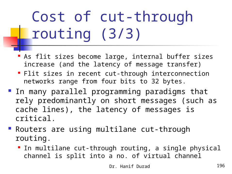
Cost of cut-through routing (3/3) As flit sizes become large, internal buffer sizes increase (and
the latency of message transfer) Flit sizes in recent cut-through interconnection networks range
from four bits to 32 bytes. In many parallel programming paradigms that rely
predominantly on short messages (such as cache lines), the latency of messages is critical.
Routers are using multilane cut-through routing. In multilane cut-through routing, a single physical channel is
split into a no. of virtual channelDr. Hanif Durad 196

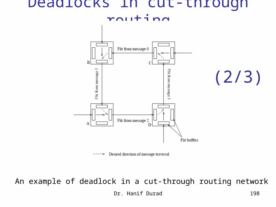
Deadlocks in cut-through routing (1/3)
While traversing the network, if a message needs to use a link that is currently in use, then the message is blocked.
This may lead to deadlock. Fig. illustrates a deadlock in a cut through routing
network The destinations of messages 0, 1, 2, and 3 are A, B, C, and D,
respectively. A flit from message 0 occupies the link CB (and the associated
buffers).
Dr. Hanif Durad 197
Dr. Hanif Durad 198
Deadlocks in cut-through routing
An example of deadlock in a cut-through routing network
(2/3)

Deadlocks in cut-through routing (3/3)
Since link BA is occupied by a flit from message 3, the flit from message 0 is blocked.
Similarly, the flit from message 3 is blocked since link AD is in use.
No messages can progress in the network and the network is deadlocked.
Can be avoided by using appropriate routing techniques & message buffers.
199
Reducing the Cost (1/4)
The equation of cost of communicating a message between two nodes l hops away using cut-through routing implies that in order to optimize the cost of message transfers:
1. Communicate in bulk: instead of sending small messages and paying a startup cost ts for
each, aggregate small messages into a single large message and amortize the startup latency across a larger message.
Because on typical platforms such as clusters and message-passing machines, the value of ts is much larger than those of th or tw.

Reducing the Cost (2/4)
2. Minimize the volume of data. To minimize the overhead paid in terms of per-word transfer
time tw, it is desirable to reduce the volume of data communicated as much as possible.
3. Minimize distance of data transfer. Minimize the number of hops l that a message must traverse.
First two objectives s are relatively easy to achieve, third is difficult (unnecessary burden algorithm designer)
Dr. Hanif Durad 201

Reducing the Cost (3/4)
In mess-pass lib. (e.g. MPI), the programmer has little control on the mapping of processes onto physical processors. In such paradigms, while tasks might have well defined topologies
and may communicate only among neighbors in the task topology, the mapping of processes to nodes might destroy this structure
Many architectures rely on randomized (two-step) routing, A message is first sent to a random node from source and from this
intermediate node to the destination.

Reducing the Cost (4/4) This alleviates hot-spots & contention on the network. Minimizing number of hops in a randomized routing network
yields no benefits.
The per-hop time (th) is typically dominated either by the startup latency (ts)for small messages or by perword component (twm) for large messages.
Since the max no. hops (l) in most networks is relatively small, the per-hop time can be ignored
Dr. Hanif Durad 203

2.5.1.4 Simplified Cost Model (1/3)
Cost of transferring a message between two nodes on a network is given by:
It takes the same amount of time to communicate between any pair of nodes it corresponds to a completely connected network.
Instead of designing algs for each specific arch (a mesh, hypercube, or tree), we design algs with this cost model in mind & port it to any target parallel comp.
Dr. Hanif Durad 204

Simplified Cost Model (2/3)
Loss of accuracy (or fidelity) of prediction when the alg is ported from our simplified model (for a completely connected network) to an actual machine arch. If our initial assumption that the th term is typically
dominated by the ts or tw terms is valid, then the loss in accuracy should be minimal.
Dr. Hanif Durad 205

Simplified Cost Model (3/3)
Valid only for uncongested networks. Architectures have varying thresholds for when they get
congested; a linear array has a much lower threshold for congestion
than a hypercube. Valid only as long as the communication pattern does
not congest the network. Different communication patterns congest a given network
to different extents.
206

Example 2.15 Effect of congestion on communication cost (1/5)
Consider a mesh in which each node is only communicating with its nearest neighbor. Since no links in the network are used for more than
one communication, the time for this operation is ts + twm, where m is the number of words communicated.
This time is consistent with our simplified model.
Dr. Hanif Durad 207
p p

Effect of congestion on communication cost (2/5)
Consider an alternate scenario in which each node is communicating with a randomly selected node.
This randomness implies that there are p/2 communications (or p/4 bi-directional communications) occurring across any equi-partition of the machine (since the node being communicated with could be in either half with equal probability).
Dr. Hanif Durad 208

Effect of congestion on communication cost (3/5)
From our discussion of bisection width, we know that a 2-D mesh has a bisection width of .
From these two, we can infer that some links would now have to carry at least messages, assuming bi-directional communication channels.
These messages must be serialized over the link. If each message is of size m, the time for this
operation is at least
p
/4 / 4p
pp
)( s wt t m p

Effect of congestion on communication cost (4/5)
This time is not in conformity with our simplified model
For a given architecture some communication patterns can be non-congesting & others congesting
This makes the task of modeling communication costs dependent not just on the architecture, but also on the communication pattern.
To address this, we introduce the notion of effective bandwidth.

Effective Bandwidth
also known as throughput is the fraction of aggregate bandwidth delivered
by the network to an application
Dr. Hanif Durad 211

Effect of congestion on communication cost (5/5)
For communication patterns that do not congest the network, is identical to the link bandwidth
For communication operations that congest the network, is the link bandwidth scaled down by the degree of congestion on the most congested link.
Difficult to estimate: it is a function of process to node mapping, routing algorithms, & communication schedule.
Therefore, we use a lower bound on the message communication time: The associated link bandwidth is scaled down by a factor p/b, b is the bisection width of the network.

2.5.2 Cost Models for Shared Address Space Machines (1/3)
Difficulty reasons: Memory layout is typically determined by the system. Finite cache sizes can result in cache thrashing Overheads associated with invalidate and update operations
are difficult to quantify Spatial locality is difficult to model Prefetching can play a role in reducing the overhead
associated with data access. False sharing and contention are difficult to model. Contention in shared accesses is often a major contributing
overhead in shared address space machines.

Cost Models for Shared Address Space Machines (2/3)
Building these into a single cost model results in a model that is too cumbersome to design programs for and too specific to individual machines to be generally
applicable. A simplified model presented above accounts
primarily for remote data access but does not model a variety of other overheads (see the textbook)
214

Cost Models for Shared Address Space Machines (3/3)
Accurate cost model for shared memory communication is difficult Same equation
can applied keeping in mind difference that the value of the constant ts relative to tw is likely to be much
smaller on a shared-memory machine than on a distributed memory machine (tw is likely to be near zero for a UMA machine).

2.6 Routing Mechanisms for Interconnection Networks (1/4)
Critical to the performance of parallel computers A routing mechanism
Determine the path a message takes through the network to get from source to destination
It takes as input a message's source and destination nodes It may also use information about the state of the network It returns one or more paths through the network from the source
to the destination

Routing Mechanisms for Interconnection Networks (2/4)
Classification based on route selection: A minimal routing mechanism
always selects one of the shortest paths between the source and the destination.
each link brings a message closer to its destination, can lead to congestion in parts of the network.
A non-minimal routing scheme may route the message along a longer path to avoid network
congestion.

Routing Mechanisms for Interconnection Networks (3/4)
Classification on the basis on information regarding the state of the network A deterministic routing scheme
determines a unique path for a message, based on its source and destination.
It does not use any information regarding the state of the network.
may result in uneven use of the communication resources in a network.
Routing Mechanisms for Interconnection Networks (4/4)
An adaptive routing scheme uses information regarding the current state of the netw to
determine the path of the mes detects congestion in the network and routes messages around it

Dimension-Ordered Routing (DOR)
Commonly used deterministic minimal routing technique
Assigns successive channels for traversal by a message based on a numbering scheme determined by the dimension of the channel.
For a two-dimensional mesh is called XY-routing For a hypercube is called E-cube routing
Dr. Hanif Durad 220

DOR XY-Routing (1/2)
Consider a two-dimensional mesh without wraparound connections.
A message is sent first along the X dimension until it reaches the column of the destination node and then along the Y dimension until it reaches its destination.
Let PSy,Sx represent the position of the source node and PDy,Dx represent that of the destination node.
Any minimal routing scheme should return a path of length |Sx - Dx| + |Sy - Dy|.
Dr. Hanif Durad 221

DOR XY-Routing (2/2)
Assume that Dx Sx and Dy Sy. The message is passed through intermediate nodes
PSy,Sx+1, PSy,Sx+2, ..., PSy,Dx along the X dimension and
Then through nodes PSy+1,Dx, PSy+2,Dx, ..., PDy,Dx along the Y dimension to reach the destination
Note that the length of this path is indeed Sx - Dx| + |Sy - Dy|.
Dr. Hanif Durad 222

E-cube Routing (1/4)
Consider a d-dimensional hypercube of p nodes. Let Ps and Pd be the labels of the source and destination
nodes We know that the binary representations of these labels
are d bits long. The minimum distance between these nodes is given by
the number of ones in Ps Pd , where represents the bitwise exclusive-OR operation.
Dr. Hanif Durad 223

E-cube Routing (2/4)
Node Ps computes Ps Pd and sends the message along dimension k, where k is the position of the least significant nonzero bit in Ps Pd .
At each intermediate step, node Pi , which receives the message, computes Pi Pd and forwards the message along the dimension corresponding to the least significant nonzero bit.
This process continues until the message reaches its destination.
Dr. Hanif Durad 224

E-cube routing- Example (3/4)
Let Ps = 010 and Pd = 111 represent the source and destination nodes for a message.
Node Ps computes 010 111 = 101.
In the first step, Ps forwards the message along the dimension corresponding to the least significant bit to node 011.
Node 011 sends the message along the dimension corresponding to the most significant bit (011 111 = 100)
The message reaches node 111, which is the destination of the message.

Dr. Hanif Durad 226
E-cube routing- Example (4/4)
Routing a message from node Ps (010) to node Pd (111) in a three-dimensional hypercube using E-cube routing.

2.7 Impact of Process-Processor Mapping (1/4)
programmer often does not have control over how logical processes are mapped to physical nodes in a network
For this reason, even communication patterns that are not inherently congesting may congest the network.
We illustrate this with the following example:
Dr. Hanif Durad 227

Impact of Process-Processor Mapping (2/4)
Problem: A programmer often does not have control over
how logical processes are mapped to physical nodes in a network. even communication patterns that are not inherently
congesting may congest the network
Dr. Hanif Durad 228

Impact of Process-Processor Mapping (3/4)
Dr. Hanif Durad 229
Processes and their interactions
Processors
G (E,V)G′(E′,V′)

Impact of process mapping (4/4)
An intuitive mapping of processes to nodes
a single link in the underlying architecture only carries data corresponding to a single communication channel between processes.
a random mapping of processes to nodes
each link in the machine carries up to six channels of data between processes.considerably larger communication times if the required data rates on communication channels between processes is high
Congestion=1Congestion=6 ?Map a=1, b=6
Dr. Hanif Durad 231
2.7.1 Mapping Techniques for Graphs
Often, we need to embed a known communication pattern into a given interconnection topology. We may have an algorithm designed for one network, which we are porting to another topology.
For these reasons, it is useful to understand mapping between graphs.
Mapping Techniques for Graphs
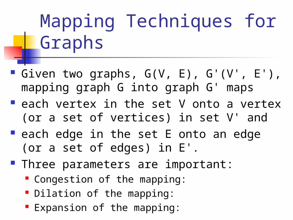
Given two graphs, G(V, E), G'(V', E'), mapping graph G into graph G' maps
each vertex in the set V onto a vertex (or a set of vertices) in set V' and
each edge in the set E onto an edge (or a set of edges) in E'.
Three parameters are important: Congestion of the mapping: Dilation of the mapping: Expansion of the mapping:

2.7.1 Mapping Techniques for Graphs
Congestion of the mapping: The maximum number of edges in E mapped onto any edge in E' it is possible that more than one edge in E is mapped onto a
single edge in E'. Dilatation of the mapping:
The maximum number of edges in E' that any edge in E is mapped onto
An edge in E may be mapped onto multiple contiguous edges in E'. This is significant because traffic on the corresponding communication
link must traverse more than one link, possibly contributing to congestion on the network.
233

Mapping Techniques for Graphs
Expansion of the mapping: It is the ratio of the number of nodes in the set V' to
that in set V The sets V and V' may contain different numbers of
vertices. In this case, a node in V corresponds to more than one node in V'.
In the context of process-processor mapping, the expansion of the mapping must be identical to the ratio of virtual & physical processors.
Dr. Hanif Durad 234

Embedding a logical topology into a physical topology
Example: embedding a 7 node binary tree into 3x3 mesh
Embedding = node mapping + edge mapping
Behrooz,P-263
G (E,V) G′(E′,V′)

Embedding a logical topology into a physical topology
Example: embedding a 7 node binary tree into 2x4 mesh
Embedding = node mapping + edge mapping
Behrooz,P-263
G (E,V)
G′(E′,V′)

Embedding a logical topology into a physical topology
Example: embedding a 7 node binary tree into 2x2 meshEmbedding = node mapping + edge mapping
Behrooz,P-263
G (E,V)G′(E′,V′)
Dilation =?

Properties of embeddings
2D-mesh Sizes 3x3 2x4 2x2
Congestion: maximum number of logical edges (joining processes) mapped onto one physical edge (joining processors) (sort of edge ratio)
1 2 2
Dilation: length of the longest path to which a logical edge (joining processes) is mapped
1 2 1
Load Factor: maximum number of logicalnodes (processes) mapped onto one physical node (processor) (sort node ratio)
1 1 2
Expansion: ratio of the number of nodes in the two topologies (over all node ratio)
9/7 8/7 4/7?

2.7.1.1 Embedding a Linear Array into a Hypercube (1/5)
Dr. Hanif Durad 239
Meshcube.pdf, P-1

Dr. Hanif Durad 240
Embedding a Linear Array into a Hypercube (2/5)
A linear array (or a ring) composed of 2d nodes (0 :2d − 1) can be embedded into a d-dimensional hypercube by mapping node i of the linear array onto node G(i, d) of the hypercube
The function G(i, x) is defined as follows:
0

Dr. Hanif Durad 241
Embedding a Linear Array into a Hypercube (3/5)
G : the binary reflected Gray code (RGC). The entry G(i, d) denotes the ith entry in the sequence of
Gray codes of d bits. Gray codes of d + 1 bits are derived from Gray codes of
d bits by reflecting the table & prefixing the reflected entries with a 1 & the original entries with a 0.
Adjoining entries (G(i, d) and G(i + 1, d)) differ from each other at only one bit position.

Dr. Hanif Durad 242
Embedding a Linear Array into a Hypercube (4/5)
Node i in the linear array is mapped to node G(i, d), and node i + 1 is mapped to G(i + 1, d) is a direct link in the hypercube that corresponds to each direct link in the linear array.
Mapping specified by the function G has a dilation of one and a congestion of one.

Dr. Hanif Durad 243
Embedding a Linear Array into a Hypercube: Example
(a) A three-bit reflected Gray code ring; and (b) its embedding into a three-dimensional hypercube.
Dilation 1
Congestion 1
(5/5)

Dr. Hanif Durad 244
2.7.1.2 Embedding a Mesh into a Hypercube (1/4)
A 2r × 2s wraparound mesh can be mapped to a 2r+s-node hypercube by mapping node (i, j) of the mesh onto node G(i, r) || G(j, s) of the hypercube (where || denotes concatenation of the two Gray codes).
Note :Mistake in book

Dr. Hanif Durad 245
Embedding a Mesh into a Hypercube
(a) A 4 × 4 mesh illustrating the mapping of mesh nodes to the nodes in a four-dimensional hypercube;
(2/4)

Embedding a Mesh into a Hypercube
(a) A 4 × 4 mesh illustrating the mapping of mesh nodes to the nodes in a four-dimensional hypercube;
A 4-Dimensional hypercube4 × 4 mesh
A better presentation workout mapping yourself (?)
Dilation 1
Congestion 1communication.pdf, P-7
(3/4)

Dr. Hanif Durad 247
Embedding a Mesh into a Hypercube
(b) a 2 × 4 mesh embedded into a three-dimensional hypercube.
Once again, the congestion, dilation, and expansion of the mapping is 1
(4/4)

Dr. Hanif Durad 248
2.7.1.3 Embedding a Mesh into a Linear Array (1/5)
An intuitive mapping of a linear array into a mesh is illustrated in Figure (a): the solid lines correspond to links in the linear array
and normal lines to links in the mesh. congestion-one, dilation-one mapping of a linear
array to a mesh is possible

Dr. Hanif Durad 249
Embedding a Mesh into a Linear Array: Example
(a) Embedding a 16 node linear array into a 2-D mesh; Solid lines correspond to links in the linear array and normal lines to links in the mesh.
Dilation 1
Congestion 1
(2/5)

Dr. Hanif Durad 250
Embedding a Mesh into a Linear Array (3/5)
Consider now the inverse of this mapping, given a mesh, map vertices of the mesh to those in a linear
array using the inverse of the same mapping function-Fig. (b) solid lines correspond to edges in the linear array and normal
lines to edges in the mesh. the congestion of the mapping in this case is five – i.e., no
solid line carries more than five normal In general: the congestion of this (inverse) mapping is +1
for a general p-node mapping (one for each of the edges to the next row, and one additional edge).

Dr. Hanif Durad 251
Embedding a Mesh into a Linear Array: Example
(b) the inverse of the mapping. Solid lines correspond to links in the linear array and normal lines to links in the mesh.
(4/5)

Embedding a Mesh into a Linear Array (5/5)
We can do better? Congestion of any mapping is lower bounded by
see textbook – why
In general: the lower bound on congestion of a mapping of network
S with x links into network Q with y links is x/y. In the case of the mapping from a mesh to a linear array,
this would be 2p/p, or 2. see textbook – why not?

Dr. Hanif Durad 253
2.7.1.4 Embedding a Hypercube into a 2-D Mesh (1/3)
p-node hypercube into a p-node 2-D mesh, p is an even power of two
visualize the hypercube as subcubes, each with nodes. let d = log p be the dim of the hypercube . take the d/2 least significant bits and use them to define individual
subcubes of nodes. For example, in the case of a 4D hypercube, we use the lower two
bits to define the subcubes as (0000, 0001, 0011, 0010), (0100, 0101, 0111, 0110), (1100, 1101, 1111, 1110), and (1000, 1001, 1011, 1010).

Dr. Hanif Durad 254
Embedding a Hypercube into a 2-D Mesh (2/3)
The (row) mapping from a hypercube to a mesh can now be defined as follows:
Each node subcube is mapped to a node row of the mesh. We do this by simply inverting the linear-array to hypercube mapping. The congestion: /2
Fig: p = 16 and p = 32 Column mapping:
We map the hypercube nodes into the mesh in such a way that nodes with identical d/2 least significant bits in the hypercube are mapped to the same column.
The congestion: /2

Dr. Hanif Durad 255
Embedding a Hypercube into a 2-D Mesh: Example
Embedding a hypercube into a 2-D mesh.
Congestion /2
(3/3)
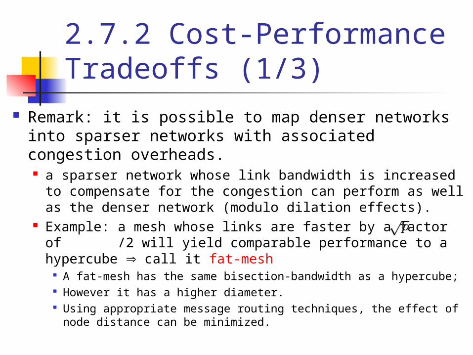
2.7.2 Cost-Performance Tradeoffs (1/3)
Remark: it is possible to map denser networks into sparser networks with associated congestion overheads. a sparser network whose link bandwidth is increased to
compensate for the congestion can perform as well as the denser network (modulo dilation effects).
Example: a mesh whose links are faster by a factor of /2 will yield comparable performance to a hypercube call it fat-mesh
A fat-mesh has the same bisection-bandwidth as a hypercube; However it has a higher diameter. Using appropriate message routing techniques, the effect of node distance
can be minimized.

Cost-Performance Tradeoffs (2/3)
Analyzing the performance of a mesh & a hypercube network with identical costs: Cost of a network is proportional to the number of
wires, A -node wraparound mesh with (log p)/4 wires per
channel costs as much as a p-node hypercube with one wire per channel
Average communication times of these two networks. See textbook

Cost-Performance Tradeoffs (3/3)
For p > 16 and sufficiently large message sizes, a mesh outperforms a hypercube of the same cost. For large enough messages, a mesh is always better than a
hypercube of the same cost, provided the network is lightly loaded.
Even when the network is heavily loaded, the performance of a mesh is similar to that of a hypercube of the same cost.

Dr. Hanif Durad 259
Case Studies: The IBM Blue-Gene Architecture
The hierarchical architecture of Blue Gene.

Dr. Hanif Durad 260
Case Studies:The Cray T3E Architecture
Interconnection network of the Cray T3E: (a) node architecture; (b) network topology

Dr. Hanif Durad 261
Case Studies: The SGI Origin 3000 Architecture
Architecture of the SGI Origin 3000 family of servers.

Dr. Hanif Durad 262
Case Studies: The Sun HPC Server Architecture
Architecture of the Sun Enterprise family of servers.

Self Study
1. Chapter 4- Advanced computer architecture and parallel processing by Hesham and Mostafa (provided in soft form on data server folder)
2. Chapter 2 - Handbook of Parallel Computing and Statistic (provided in soft form on data server folder)
Dr. Hanif Durad 263