Embed Size (px)
Citation preview

© 2012 McGraw-Hill Education (Asia)Garrison, Noreen, Brewer, Cheng & Yuen
Standard Costs and Operating
Performance Measures
Chapter 12

McGraw-Hill Education (Asia) Garrison, Noreen, Brewer, Cheng & YuenMcGraw-Hill/Irwin Slide 2
Standard Costs
Standards are benchmarks or “norms” for
measuring performance. In managerial accounting,
two types of standards are commonly used.
Quantity standards
specify how much of an
input should be used to
make a product or
provide a service.
Price standards
specify how much
should be paid for
each unit of the
input.
Examples: Firestone, Sears, McDonald’s, hospitals,
construction and manufacturing companies.

McGraw-Hill Education (Asia) Garrison, Noreen, Brewer, Cheng & YuenMcGraw-Hill/Irwin Slide 3
Standard Costs
DirectMaterial
Deviations from standards deemed significant
are brought to the attention of management, a
practice known as management by exception.
Type of Product Cost
Am
ou
nt
DirectLabor
ManufacturingOverhead
Standard

McGraw-Hill Education (Asia) Garrison, Noreen, Brewer, Cheng & YuenMcGraw-Hill/Irwin Slide 4
Variance Analysis Cycle
Prepare standard
cost performance
report
Analyze
variances
Begin
Identify
questions
Receive
explanations
Take
corrective
actions
Conduct next
period’s
operations

McGraw-Hill Education (Asia) Garrison, Noreen, Brewer, Cheng & YuenMcGraw-Hill/Irwin Slide 5
Accountants, engineers, purchasing
agents, and production managers
combine efforts to set standards that encourage
efficient future operations.
Setting Standard Costs

McGraw-Hill Education (Asia) Garrison, Noreen, Brewer, Cheng & YuenMcGraw-Hill/Irwin Slide 6
Setting Standard Costs
Should we use
ideal standards that
require employees to
work at 100 percent
peak efficiency?
Engineer Managerial Accountant
I recommend using practical
standards that are currently
attainable with reasonable
and efficient effort.

McGraw-Hill Education (Asia) Garrison, Noreen, Brewer, Cheng & YuenMcGraw-Hill/Irwin Slide 7
Learning Objective 1
Explain how direct
materials standards and
direct labor
standards are set.

McGraw-Hill Education (Asia) Garrison, Noreen, Brewer, Cheng & YuenMcGraw-Hill/Irwin Slide 8
Setting Direct Material Standards
Price
Standards
Summarized in
a Bill of Materials.
Final, delivered
cost of materials,
net of discounts.
Quantity
Standards

McGraw-Hill Education (Asia) Garrison, Noreen, Brewer, Cheng & YuenMcGraw-Hill/Irwin Slide 9
Setting Standards
Six Sigma advocates have sought to
eliminate all defects and waste, rather than
continually build them into standards.
As a result allowances for waste and
spoilage that are built into standards
should be reduced over time.

McGraw-Hill Education (Asia) Garrison, Noreen, Brewer, Cheng & YuenMcGraw-Hill/Irwin Slide 10
Setting Direct Labor Standards
Rate
Standards
Often a single
rate is used that reflects
the mix of wages earned.
Time
Standards
Use time and
motion studies for
each labor operation.
McGraw-Hill Education (Asia) Garrison, Noreen, Brewer, Cheng & YuenMcGraw-Hill/Irwin Slide 11
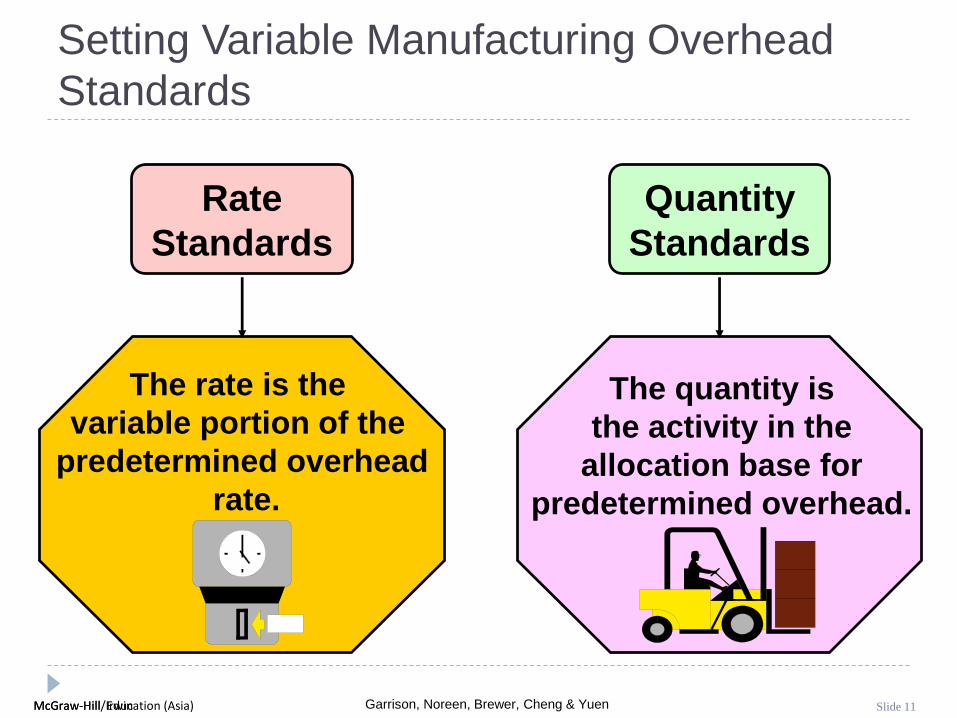
Setting Variable Manufacturing Overhead
Standards
Rate
Standards
The rate is the
variable portion of the
predetermined overhead
rate.
Quantity
Standards
The quantity is
the activity in the
allocation base for
predetermined overhead.

McGraw-Hill Education (Asia) Garrison, Noreen, Brewer, Cheng & YuenMcGraw-Hill/Irwin Slide 12
Standard Cost Card – Variable Production Cost
A standard cost card for one unit of
product might look like this:
A A x B
Standard Standard Standard
Quantity Price Cost
Inputs or Hours or Rate per Unit
Direct materials 3.0 lbs. 4.00$ per lb. 12.00$
Direct labor 2.5 hours 14.00 per hour 35.00
Variable mfg. overhead 2.5 hours 3.00 per hour 7.50
Total standard unit cost 54.50$
B

McGraw-Hill Education (Asia) Garrison, Noreen, Brewer, Cheng & YuenMcGraw-Hill/Irwin Slide 13
Price and Quantity Standards
Price and quantity standards are
determined separately for two reasons:
The purchasing manager is responsible for raw
material purchase prices and the production manager
is responsible for the quantity of raw material used.
The buying and using activities occur at different times.
Raw material purchases may be held in inventory for a
period of time before being used in production.

McGraw-Hill Education (Asia) Garrison, Noreen, Brewer, Cheng & YuenMcGraw-Hill/Irwin Slide 14
A General Model for Variance Analysis
Variance Analysis
Price Variance
Difference between
actual price and
standard price
Quantity Variance
Difference between
actual quantity and
standard quantity

McGraw-Hill Education (Asia) Garrison, Noreen, Brewer, Cheng & YuenMcGraw-Hill/Irwin Slide 15
Variance Analysis
Materials price variance
Labor rate variance
VOH rate variance
Materials quantity variance
Labor efficiency variance
VOH efficiency variance
A General Model for Variance Analysis
Price Variance Quantity Variance

McGraw-Hill Education (Asia) Garrison, Noreen, Brewer, Cheng & YuenMcGraw-Hill/Irwin Slide 16
Price Variance Quantity Variance
Actual Quantity Actual Quantity Standard Quantity× × ×
Actual Price Standard Price Standard Price
A General Model for Variance Analysis

McGraw-Hill Education (Asia) Garrison, Noreen, Brewer, Cheng & YuenMcGraw-Hill/Irwin Slide 17
Price Variance Quantity Variance
Actual Quantity Actual Quantity Standard Quantity× × ×
Actual Price Standard Price Standard Price
A General Model for Variance Analysis
Actual quantity is the amount of direct
materials, direct labor, and variable
manufacturing overhead actually used.

McGraw-Hill Education (Asia) Garrison, Noreen, Brewer, Cheng & YuenMcGraw-Hill/Irwin Slide 18
Price Variance Quantity Variance
Actual Quantity Actual Quantity Standard Quantity× × ×
Actual Price Standard Price Standard Price
A General Model for Variance Analysis
Standard quantity is the standard quantity
allowed for the actual output of the period.
McGraw-Hill Education (Asia) Garrison, Noreen, Brewer, Cheng & YuenMcGraw-Hill/Irwin Slide 19
Price Variance Quantity Variance
Actual Quantity Actual Quantity Standard Quantity× × ×
Actual Price Standard Price Standard Price
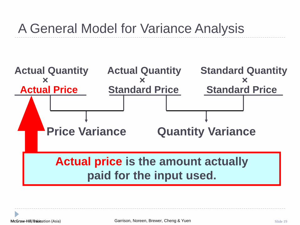
A General Model for Variance Analysis
Actual price is the amount actually
paid for the input used.

McGraw-Hill Education (Asia) Garrison, Noreen, Brewer, Cheng & YuenMcGraw-Hill/Irwin Slide 20
A General Model for Variance Analysis
Standard price is the amount that should
have been paid for the input used.
Price Variance Quantity Variance
Actual Quantity Actual Quantity Standard Quantity× × ×
Actual Price Standard Price Standard Price

McGraw-Hill Education (Asia) Garrison, Noreen, Brewer, Cheng & YuenMcGraw-Hill/Irwin Slide 21
A General Model for Variance Analysis
(AQ × AP) – (AQ × SP) (AQ × SP) – (SQ × SP)
AQ = Actual Quantity SP = Standard Price
AP = Actual Price SQ = Standard Quantity
Price Variance Quantity Variance
Actual Quantity Actual Quantity Standard Quantity× × ×
Actual Price Standard Price Standard Price
McGraw-Hill Education (Asia) Garrison, Noreen, Brewer, Cheng & YuenMcGraw-Hill/Irwin Slide 22
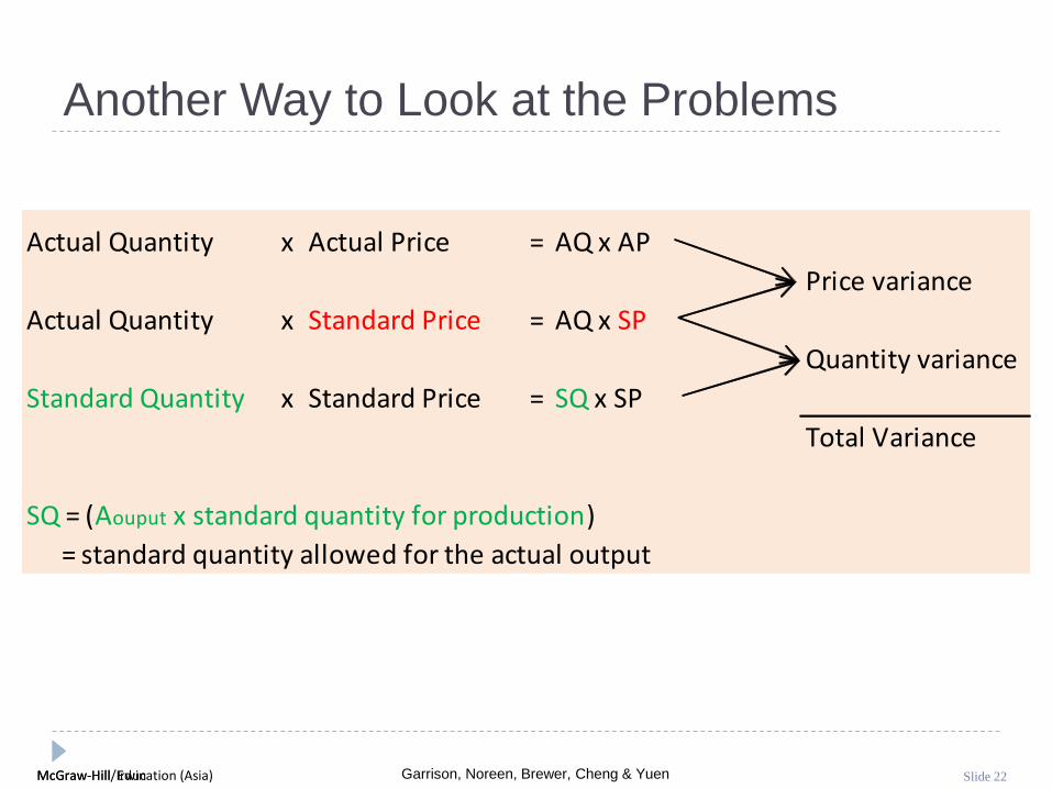
Another Way to Look at the Problems
Actual Quantity x Actual Price = AQ x AP
Price variance
Actual Quantity x Standard Price = AQ x SP
Quantity variance
Standard Quantity x Standard Price = SQ x SP
Total Variance
SQ = (Aouput x standard quantity for production)
= standard quantity allowed for the actual output

McGraw-Hill Education (Asia) Garrison, Noreen, Brewer, Cheng & YuenMcGraw-Hill/Irwin Slide 23
Learning Objective 2
Compute the direct
materials price and
quantity variances and
explain their significance.

McGraw-Hill Education (Asia) Garrison, Noreen, Brewer, Cheng & YuenMcGraw-Hill/Irwin Slide 24
Glacier Peak Outfitters has the following direct
material standard for the fiberfill in its mountain
parka.
0.1 kg. of fiberfill per parka at $5.00 per kg.
Last month 210 kgs. of fiberfill were purchased and
used to make 2,000 parkas. The material cost a
total of $1,029.
Material Variances – An Example

McGraw-Hill Education (Asia) Garrison, Noreen, Brewer, Cheng & YuenMcGraw-Hill/Irwin Slide 25
Material Variances: The Line-by-line Method
AQ x AP = 210 x AP = 1,029
(21) F Price variance
AQ x SP = 210 x 5 = 1,050
50 U Quantity variance
SQ x SP = (2000 x 0.1) x 5 = 1,000
29 U Total Variance
SQ = (Aouput x standard quantity for production)
= standard quantity allowed for the actual output
Calculation of Actual Purchase Price (AP) per unit can be done but is
not necessary because AP will not be used in subsequent calculation
and the total actual purchase cost in total is sufficient for the variance
calculation.

McGraw-Hill Education (Asia) Garrison, Noreen, Brewer, Cheng & YuenMcGraw-Hill/Irwin Slide 26
210 kgs. 210 kgs. 200 kgs.
× × ×
$4.90 per kg. $5.00 per kg. $5.00 per kg.
= $1,029 = $1,050 = $1,000
Price variance
$21 favorable
Quantity variance
$50 unfavorable
Actual Quantity Actual Quantity Standard Quantity× × ×
Actual Price Standard Price Standard Price
Material Variances Summary

McGraw-Hill Education (Asia) Garrison, Noreen, Brewer, Cheng & YuenMcGraw-Hill/Irwin Slide 27
210 kgs. 210 kgs. 200 kgs.
× × ×
$4.90 per kg. $5.00 per kg. $5.00 per kg.
= $1,029 = $1,050 = $1,000
Price variance
$21 favorable
Quantity variance
$50 unfavorable
Actual Quantity Actual Quantity Standard Quantity× × ×
Actual Price Standard Price Standard Price
$1,029 210 kgs
= $4.90 per kg
Material Variances Summary

McGraw-Hill Education (Asia) Garrison, Noreen, Brewer, Cheng & YuenMcGraw-Hill/Irwin Slide 28
210 kgs. 210 kgs. 200 kgs.
× × ×
$4.90 per kg. $5.00 per kg. $5.00 per kg.
= $1,029 = $1,050 = $1,000
Price variance
$21 favorable
Quantity variance
$50 unfavorable
Actual Quantity Actual Quantity Standard Quantity× × ×
Actual Price Standard Price Standard Price
0.1 kg per parka 2,000 parkas
= 200 kgs
Material Variances Summary

McGraw-Hill Education (Asia) Garrison, Noreen, Brewer, Cheng & YuenMcGraw-Hill/Irwin Slide 29
Material Variances:Using the Factored Equations
Materials price variance
MPV = AQ (AP - SP)
= 210 kgs ($4.90/kg - $5.00/kg)
= 210 kgs (-$0.10/kg)
= $21 F
Materials quantity variance
MQV = SP (AQ - SQ)
= $5.00/kg (210 kgs-(0.1 kg/parka 2,000 parkas))
= $5.00/kg (210 kgs - 200 kgs)
= $5.00/kg (10 kgs)
= $50 U

McGraw-Hill Education (Asia) Garrison, Noreen, Brewer, Cheng & YuenMcGraw-Hill/Irwin Slide 30
Isolation of Material Variances
I need the price variancesooner so that I can better
identify purchasing problems.
You accountants just don’tunderstand the problems thatpurchasing managers have.
I’ll start computing
the price variance
when material is
purchased rather
than when it’s used.

McGraw-Hill Education (Asia) Garrison, Noreen, Brewer, Cheng & YuenMcGraw-Hill/Irwin Slide 31
Material Variances
Hanson purchased and used 1,700 pounds.
How are the variances computed if the amount purchased differs from
the amount used?
The price variance is computed on the entire
quantity purchased.
The quantity variance is computed only on
the quantity used.
McGraw-Hill Education (Asia) Garrison, Noreen, Brewer, Cheng & YuenMcGraw-Hill/Irwin Slide 32
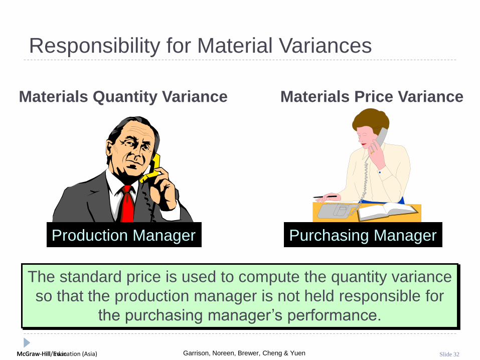
Materials Price VarianceMaterials Quantity Variance
Production Manager Purchasing Manager
The standard price is used to compute the quantity variance
so that the production manager is not held responsible for
the purchasing manager’s performance.
Responsibility for Material Variances

McGraw-Hill Education (Asia) Garrison, Noreen, Brewer, Cheng & YuenMcGraw-Hill/Irwin Slide 33
I am not responsible forthis unfavorable material
quantity variance.
You purchased cheapmaterial, so my peoplehad to use more of it.
Your poor scheduling sometimes requires me to
rush order material at a higher price, causing
unfavorable price variances.
Responsibility for Material Variances

McGraw-Hill Education (Asia) Garrison, Noreen, Brewer, Cheng & YuenMcGraw-Hill/Irwin Slide 34
Hanson Inc. has the following direct material standard to manufacture one Zippy:
1.5 pounds per Zippy at $4.00 per pound
Last week, 1,700 pounds of material were purchased and used to make 1,000 Zippies. The
material cost a total of $6,630.
Zippy
Quick Check

McGraw-Hill Education (Asia) Garrison, Noreen, Brewer, Cheng & YuenMcGraw-Hill/Irwin Slide 35
Quick Check
AQ x AP = 1,700 x AP = 6,630
(170) F Price variance
AQ x SP = 1,700 x 4 = 6,800
800 U Quantity variance
SQ x SP = (1000 x 1.5) x 4 = 6,000
630 U Total Variance
SQ = (Aouput x standard quantity for production)
= standard quantity allowed for the actual output
Zippy

McGraw-Hill Education (Asia) Garrison, Noreen, Brewer, Cheng & YuenMcGraw-Hill/Irwin Slide 36
Quick Check Zippy
Hanson’s material price variance (MPV)
for the week was:
a. $170 unfavorable.
b. $170 favorable.
c. $800 unfavorable.
d. $800 favorable.

McGraw-Hill Education (Asia) Garrison, Noreen, Brewer, Cheng & YuenMcGraw-Hill/Irwin Slide 37
Hanson’s material price variance (MPV)
for the week was:
a. $170 unfavorable.
b. $170 favorable.
c. $800 unfavorable.
d. $800 favorable.
MPV = AQ(AP - SP)
MPV = 1,700 lbs. × ($3.90 - 4.00)
MPV = $170 Favorable
Quick Check Zippy
AQ x AP = 1,700 x AP = 6,630
(170) F Price variance
AQ x SP = 1,700 x 4 = 6,800

McGraw-Hill Education (Asia) Garrison, Noreen, Brewer, Cheng & YuenMcGraw-Hill/Irwin Slide 38
Quick Check
Hanson’s material quantity variance (MQV)
for the week was:
a. $170 unfavorable.
b. $170 favorable.
c. $800 unfavorable.
d. $800 favorable.
Zippy

McGraw-Hill Education (Asia) Garrison, Noreen, Brewer, Cheng & YuenMcGraw-Hill/Irwin Slide 39
Hanson’s material quantity variance (MQV)
for the week was:
a. $170 unfavorable.
b. $170 favorable.
c. $800 unfavorable.
d. $800 favorable.MQV = SP(AQ - SQ)
MQV = $4.00(1,700 lbs - 1,500 lbs)
MQV = $800 unfavorable
Quick Check Zippy
AQ x SP = 1,700 x 4 = 6,800
800 U Quantity variance
SQ x SP = (1000 x 1.5) x 4 = 6,000

McGraw-Hill Education (Asia) Garrison, Noreen, Brewer, Cheng & YuenMcGraw-Hill/Irwin Slide 40
1,700 lbs. 1,700 lbs. 1,500 lbs.
× × ×
$3.90 per lb. $4.00 per lb. $4.00 per lb.
= $6,630 = $ 6,800 = $6,000
Price variance
$170 favorable
Quantity variance
$800 unfavorable
Actual Quantity Actual Quantity Standard Quantity× × ×
Actual Price Standard Price Standard Price
Zippy
Quick Check

McGraw-Hill Education (Asia) Garrison, Noreen, Brewer, Cheng & YuenMcGraw-Hill/Irwin Slide 41
Hanson Inc. has the following material standard to
manufacture one Zippy:
1.5 pounds per Zippy at $4.00 per pound
Last week, 2,800 pounds of material were
purchased at a total cost of $10,920, and 1,700
pounds were used to make 1,000 Zippies.
Zippy
Quick Check Continued

McGraw-Hill Education (Asia) Garrison, Noreen, Brewer, Cheng & YuenMcGraw-Hill/Irwin Slide 42
Quick Check Continued
AQp x AP = 2,800 x AP = 10,920
(280) F Price variance
AQp x SP = 2,800 x 4 = 11,200
4,400 U Inventory @ Std cost
AQu x SP = 1,700 x 4 = 6,800
800 U Usage variance
SQ x SP = (1000 x 1.5) x 4 = 6,000 (Quantity variance)
4,920 U Total Variance
AQp = Actual Quantity Purchased
AQu = Actual Quantity used
SQ = (Aouput x standard quantity for production use)
= standard quantity allowed for the actual output
Zippy

McGraw-Hill Education (Asia) Garrison, Noreen, Brewer, Cheng & YuenMcGraw-Hill/Irwin Slide 43
Actual Quantity Actual QuantityPurchased Purchased
× ×Actual Price Standard Price
2,800 lbs. 2,800 lbs.
× ×
$3.90 per lb. $4.00 per lb.
= $10,920 = $11,200
Price variance
$280 favorable
Price variance increases
because quantity
purchased increases.
Zippy
Quick Check Continued

McGraw-Hill Education (Asia) Garrison, Noreen, Brewer, Cheng & YuenMcGraw-Hill/Irwin Slide 44
Actual QuantityUsed Standard Quantity
× ×Standard Price Standard Price
1,700 lbs. 1,500 lbs.
× ×
$4.00 per lb. $4.00 per lb.
= $6,800 = $6,000
Quantity variance
$800 unfavorable
Quantity variance is
unchanged because
actual and standard
quantities are unchanged.
Zippy
Quick Check Continued

McGraw-Hill Education (Asia) Garrison, Noreen, Brewer, Cheng & YuenMcGraw-Hill/Irwin Slide 45
Learning Objective 3
Compute the direct labor
rate and efficiency
variances and explain
their significance.

McGraw-Hill Education (Asia) Garrison, Noreen, Brewer, Cheng & YuenMcGraw-Hill/Irwin Slide 46
Glacier Peak Outfitters has the following direct labor
standard for its mountain parka.
1.2 standard hours per parka at $10.00 per hour
Last month, employees actually worked 2,500 hours
at a total labor cost of $26,250 to make 2,000
parkas.
Labor Variances – An Example

McGraw-Hill Education (Asia) Garrison, Noreen, Brewer, Cheng & YuenMcGraw-Hill/Irwin Slide 47
Labor Variances
AH x AR = 2,500 x AR = 26,250
1,250 U Rate variance
AH x SR = 2,500 x 10 = 25,000
1,000 U Efficiency variance
SH x SR = (2000 x 1.2) x 10 = 24,000
2,250 U Total Variance
AH = Actual hour paid (and worked in this case)
AR = Actual rate per hour
SR = Standard rate per hour
SH = (Aouput x standard hours for the production)
= standard hours allowed for the actual output

McGraw-Hill Education (Asia) Garrison, Noreen, Brewer, Cheng & YuenMcGraw-Hill/Irwin Slide 48
Rate variance
$1,250 unfavorable
Efficiency variance
$1,000 unfavorable
Actual Hours Actual Hours Standard Hours× × ×
Actual Rate Standard Rate Standard Rate
Labor Variances Summary
2,500 hours 2,500 hours 2,400 hours
× × ×
$10.50 per hour $10.00 per hour. $10.00 per hour
= $26,250 = $25,000 = $24,000

McGraw-Hill Education (Asia) Garrison, Noreen, Brewer, Cheng & YuenMcGraw-Hill/Irwin Slide 49
Labor Variances Summary
2,500 hours 2,500 hours 2,400 hours
× × ×
$10.50 per hour $10.00 per hour. $10.00 per hour
= $26,250 = $25,000 = $24,000
Actual Hours Actual Hours Standard Hours× × ×
Actual Rate Standard Rate Standard Rate
$26,250 2,500 hours
= $10.50 per hour
Rate variance
$1,250 unfavorable
Efficiency variance
$1,000 unfavorable

McGraw-Hill Education (Asia) Garrison, Noreen, Brewer, Cheng & YuenMcGraw-Hill/Irwin Slide 50
Labor Variances Summary
2,500 hours 2,500 hours 2,400 hours
× × ×
$10.50 per hour $10.00 per hour. $10.00 per hour
= $26,250 = $25,000 = $24,000
Actual Hours Actual Hours Standard Hours× × ×
Actual Rate Standard Rate Standard Rate
1.2 hours per parka 2,000
parkas = 2,400 hours
Rate variance
$1,250 unfavorable
Efficiency variance
$1,000 unfavorable

McGraw-Hill Education (Asia) Garrison, Noreen, Brewer, Cheng & YuenMcGraw-Hill/Irwin Slide 51
Labor Variances:Using the Factored Equations
Labor rate variance
LRV = AH (AR - SR)
= 2,500 hours ($10.50 per hour – $10.00 per hour)
= 2,500 hours ($0.50 per hour)
= $1,250 unfavorable
Labor efficiency variance
LEV = SR (AH - SH)
= $10.00 per hour (2,500 hours – 2,400 hours)
= $10.00 per hour (100 hours)
= $1,000 unfavorable

McGraw-Hill Education (Asia) Garrison, Noreen, Brewer, Cheng & YuenMcGraw-Hill/Irwin Slide 52
Responsibility for Labor Variances
Production Manager
Production managers are
usually held accountable
for labor variances
because they can
influence the:
Mix of skill levels
assigned to work tasks.
Level of employee
motivation.
Quality of production
supervision.
Quality of training
provided to employees.

McGraw-Hill Education (Asia) Garrison, Noreen, Brewer, Cheng & YuenMcGraw-Hill/Irwin Slide 53
I am not responsible forthe unfavorable laborefficiency variance!
You purchased cheapmaterial, so it took more
time to process it.
I think it took more time to process the
materials because the Maintenance
Department has poorly maintained your
equipment.
Responsibility for Labor Variances

McGraw-Hill Education (Asia) Garrison, Noreen, Brewer, Cheng & YuenMcGraw-Hill/Irwin Slide 54
Hanson Inc. has the following direct laborstandard to manufacture one Zippy:
1.5 standard hours per Zippy at$12.00 per direct labor hour
Last week, 1,550 direct labor hours wereworked at a total labor cost of $18,910
to make 1,000 Zippies.
Zippy
Quick Check

McGraw-Hill Education (Asia) Garrison, Noreen, Brewer, Cheng & YuenMcGraw-Hill/Irwin Slide 55
Quick Check
AH x AR = 1,550 x AR = 18,910
310 U Rate variance
AH x SR = 1,550 x 12 = 18,600
600 U Efficiency variance
SH x SR = (1000 x 1.5) x 12 = 18,000
910 U Total Variance
AH = Actual hour paid (and worked in this case)
AR = Actual rate per hour
SR = Standard rate per hour
SH = (Aouput x standard hours for the production)
= standard hours allowed for the actual output

McGraw-Hill Education (Asia) Garrison, Noreen, Brewer, Cheng & YuenMcGraw-Hill/Irwin Slide 56
Hanson’s labor rate variance (LRV) for the
week was:
a. $310 unfavorable.
b. $310 favorable.
c. $300 unfavorable.
d. $300 favorable.
Quick Check Zippy

McGraw-Hill Education (Asia) Garrison, Noreen, Brewer, Cheng & YuenMcGraw-Hill/Irwin Slide 57
Hanson’s labor rate variance (LRV) for the
week was:
a. $310 unfavorable.
b. $310 favorable.
c. $300 unfavorable.
d. $300 favorable.
Quick Check
LRV = AH(AR - SR)
LRV = 1,550 hrs($12.20 - $12.00)
LRV = $310 unfavorable
Zippy
AH x AR = 1,550 x AR = 18,910
310 U Rate variance
AH x SR = 1,550 x 12 = 18,600

McGraw-Hill Education (Asia) Garrison, Noreen, Brewer, Cheng & YuenMcGraw-Hill/Irwin Slide 58
Hanson’s labor efficiency variance (LEV)
for the week was:
a. $590 unfavorable.
b. $590 favorable.
c. $600 unfavorable.
d. $600 favorable.
Quick Check Zippy

McGraw-Hill Education (Asia) Garrison, Noreen, Brewer, Cheng & YuenMcGraw-Hill/Irwin Slide 59
Hanson’s labor efficiency variance (LEV)
for the week was:
a. $590 unfavorable.
b. $590 favorable.
c. $600 unfavorable.
d. $600 favorable.
Quick Check
LEV = SR(AH - SH)
LEV = $12.00(1,550 hrs - 1,500 hrs)
LEV = $600 unfavorable
Zippy
AH x SR = 1,550 x 12 = 18,600
600 U Efficiency variance
SH x SR = (1000 x 1.5) x 12 = 18,000

McGraw-Hill Education (Asia) Garrison, Noreen, Brewer, Cheng & YuenMcGraw-Hill/Irwin Slide 60
Actual Hours Actual Hours Standard Hours× × ×
Actual Rate Standard Rate Standard Rate
Rate variance
$310 unfavorable
Efficiency variance
$600 unfavorable
1,550 hours 1,550 hours 1,500 hours
× × ×
$12.20 per hour $12.00 per hour $12.00 per hour
= $18,910 = $18,600 = $18,000
Zippy
Quick Check

McGraw-Hill Education (Asia) Garrison, Noreen, Brewer, Cheng & YuenMcGraw-Hill/Irwin Slide 61
Learning Objective 4
Compute the variable
manufacturing overhead
rate and efficiency
variances.

McGraw-Hill Education (Asia) Garrison, Noreen, Brewer, Cheng & YuenMcGraw-Hill/Irwin Slide 62
Glacier Peak Outfitters has the following direct variable manufacturing overhead labor standard for its mountain
parka.
1.2 standard hours per parka at $4.00 per hour
Last month, employees actually worked 2,500 hours to make 2,000 parkas. Actual variable manufacturing
overhead for the month was $10,500.
Variable Manufacturing Overhead Variances – An Example

McGraw-Hill Education (Asia) Garrison, Noreen, Brewer, Cheng & YuenMcGraw-Hill/Irwin Slide 63
Variable Manufacturing Overhead Variances
AH x AR = 2,500 x AR = 10,500
500 U Rate variance
AH x SR = 2,500 x 4 = 10,000
400 U Efficiency variance
SH x SR = (2000 x 1.2) x 4 = 9,600
900 U Total Variance
AH = Actual hour paid (and worked in this case)
AR = Actual rate per hour
SR = Standard rate per hour
SH = (Aouput x standard hours for the production)
= standard hours allowed for the actual output

McGraw-Hill Education (Asia) Garrison, Noreen, Brewer, Cheng & YuenMcGraw-Hill/Irwin Slide 64
2,500 hours 2,500 hours 2,400 hours
× × ×
$4.20 per hour $4.00 per hour $4.00 per hour
= $10,500 = $10,000 = $9,600
Rate variance
$500 unfavorable
Efficiency variance
$400 unfavorable
Actual Hours Actual Hours Standard Hours× × ×
Actual Rate Standard Rate Standard Rate
Variable Manufacturing Overhead Variances Summary

McGraw-Hill Education (Asia) Garrison, Noreen, Brewer, Cheng & YuenMcGraw-Hill/Irwin Slide 65
Actual Hours Actual Hours Standard Hours× × ×
Actual Rate Standard Rate Standard Rate
2,500 hours 2,500 hours 2,400 hours
× × ×
$4.20 per hour $4.00 per hour $4.00 per hour
= $10,500 = $10,000 = $9,600
Rate variance
$500 unfavorable
Efficiency variance
$400 unfavorable
$10,500 2,500 hours
= $4.20 per hour
Variable Manufacturing Overhead Variances Summary

McGraw-Hill Education (Asia) Garrison, Noreen, Brewer, Cheng & YuenMcGraw-Hill/Irwin Slide 66
Actual Hours Actual Hours Standard Hours× × ×
Actual Rate Standard Rate Standard Rate
2,500 hours 2,500 hours 2,400 hours
× × ×
$4.20 per hour $4.00 per hour $4.00 per hour
= $10,500 = $10,000 = $9,600
Rate variance
$500 unfavorable
Efficiency variance
$400 unfavorable
1.2 hours per parka 2,000
parkas = 2,400 hours
Variable Manufacturing Overhead Variances Summary

McGraw-Hill Education (Asia) Garrison, Noreen, Brewer, Cheng & YuenMcGraw-Hill/Irwin Slide 67
Variable Manufacturing Overhead Variances: Using Factored Equations
Variable manufacturing overhead rate variance
VMRV = AH (AR - SR)
= 2,500 hours ($4.20 per hour – $4.00 per hour)
= 2,500 hours ($0.20 per hour)
= $500 unfavorable
Variable manufacturing overhead efficiency variance
VMEV = SR (AH - SH)
= $4.00 per hour (2,500 hours – 2,400 hours)
= $4.00 per hour (100 hours)
= $400 unfavorable

McGraw-Hill Education (Asia) Garrison, Noreen, Brewer, Cheng & YuenMcGraw-Hill/Irwin Slide 68
Hanson Inc. has the following variablemanufacturing overhead standard to
manufacture one Zippy:
1.5 standard hours per Zippy at$3.00 per direct labor hour
Last week, 1,550 hours were worked to make1,000 Zippies, and $5,115 was spent for
variable manufacturing overhead.
Zippy
Quick Check

McGraw-Hill Education (Asia) Garrison, Noreen, Brewer, Cheng & YuenMcGraw-Hill/Irwin Slide 69
Quick Check
AH x AR = 1,550 x AR = 5,115
465 U Rate variance
AH x SR = 1,550 x 3 = 4,650
150 U Efficiency variance
SH x SR = (1000 x 1.5) x 3 = 4,500
615 U Total Variance
AH = Actual hour paid (and worked in this case)
AR = Actual rate per hour
SR = Standard rate per hour
SH = (Aouput x standard hours for the production)
= standard hours allowed for the actual output

McGraw-Hill Education (Asia) Garrison, Noreen, Brewer, Cheng & YuenMcGraw-Hill/Irwin Slide 70
Hanson’s rate variance (VMRV) for variable
manufacturing overhead for the week was:
a. $465 unfavorable.
b. $400 favorable.
c. $335 unfavorable.
d. $300 favorable.
Quick Check Zippy

McGraw-Hill Education (Asia) Garrison, Noreen, Brewer, Cheng & YuenMcGraw-Hill/Irwin Slide 71
Hanson’s rate variance (VMRV) for variable
manufacturing overhead for the week was:
a. $465 unfavorable.
b. $400 favorable.
c. $335 unfavorable.
d. $300 favorable.
Quick Check
VMRV = AH(AR - SR)
VMRV = 1,550 hrs($3.30 - $3.00)
VMRV = $465 unfavorable
Zippy
AH x AR = 1,550 x AR = 5,115
465 U Rate variance
AH x SR = 1,550 x 3 = 4,650

McGraw-Hill Education (Asia) Garrison, Noreen, Brewer, Cheng & YuenMcGraw-Hill/Irwin Slide 72
Hanson’s efficiency variance (VMEV) for
variable manufacturing overhead for the week
was:
a. $435 unfavorable.
b. $435 favorable.
c. $150 unfavorable.
d. $150 favorable.
Quick Check Zippy

McGraw-Hill Education (Asia) Garrison, Noreen, Brewer, Cheng & YuenMcGraw-Hill/Irwin Slide 73
Hanson’s efficiency variance (VMEV) for
variable manufacturing overhead for the week
was:
a. $435 unfavorable.
b. $435 favorable.
c. $150 unfavorable.
d. $150 favorable.
Quick Check
VMEV = SR(AH - SH)
VMEV = $3.00(1,550 hrs - 1,500 hrs)
VMEV = $150 unfavorable
1,000 units × 1.5 hrs per unit
Zippy
AH x SR = 1,550 x 3 = 4,650
150 U Efficiency variance
SH x SR = (1000 x 1.5) x 3 = 4,500

McGraw-Hill Education (Asia) Garrison, Noreen, Brewer, Cheng & YuenMcGraw-Hill/Irwin Slide 74
Rate variance
$465 unfavorable
Efficiency variance
$150 unfavorable
1,550 hours 1,550 hours 1,500 hours
× × ×
$3.30 per hour $3.00 per hour $3.00 per hour
= $5,115 = $4,650 = $4,500
Actual Hours Actual Hours Standard Hours× × ×
Actual Rate Standard Rate Standard Rate
Zippy
Quick Check

McGraw-Hill Education (Asia) Garrison, Noreen, Brewer, Cheng & YuenMcGraw-Hill/Irwin Slide 75
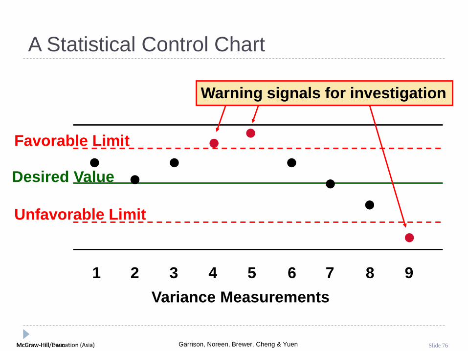
Variance Analysis and Management by Exception
How do I know
which variances to
investigate?
Larger variances, in dollar amount or as a percentage of the
standard, are investigated first.
McGraw-Hill Education (Asia) Garrison, Noreen, Brewer, Cheng & YuenMcGraw-Hill/Irwin Slide 76
A Statistical Control Chart
1 2 3 4 5 6 7 8 9
Variance Measurements
Favorable Limit
Unfavorable Limit
••
•• •
••
••
Warning signals for investigation
Desired Value
McGraw-Hill Education (Asia) Garrison, Noreen, Brewer, Cheng & YuenMcGraw-Hill/Irwin Slide 77
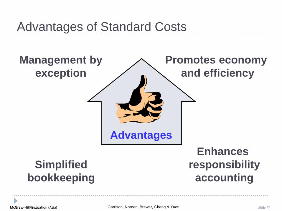
Advantages of Standard Costs
Management by
exception
Advantages
Promotes economy
and efficiency
Simplified
bookkeeping
Enhances
responsibility
accounting

McGraw-Hill Education (Asia) Garrison, Noreen, Brewer, Cheng & YuenMcGraw-Hill/Irwin Slide 78
Potential
Problems
Emphasis onnegative may
impact morale.
Emphasizing standardsmay exclude other
important objectives.
Favorablevariances may
be misinterpreted.
Continuousimprovement maybe more important
than meeting standards.
Standard costreports may
not be timely.
Invalid assumptionsabout the relationship
between laborcost and output.
Potential Problems with Standard Costs

McGraw-Hill Education (Asia) Garrison, Noreen, Brewer, Cheng & YuenMcGraw-Hill/Irwin Slide 79
Learning Objective 5
Compute delivery cycle
time, throughput time, and
manufacturing cycle
efficiency (MCE).

McGraw-Hill Education (Asia) Garrison, Noreen, Brewer, Cheng & YuenMcGraw-Hill/Irwin Slide 80
Process time is the only value-added time.
Delivery Performance Measures
Wait TimeProcess Time + Inspection Time
+ Move Time + Queue Time
Delivery Cycle Time
Order Received
ProductionStarted
Goods Shipped
Throughput Time

McGraw-Hill Education (Asia) Garrison, Noreen, Brewer, Cheng & YuenMcGraw-Hill/Irwin Slide 81
Manufacturing
Cycle
Efficiency
Value-added time
Manufacturing cycle time=
Wait TimeProcess Time + Inspection Time
+ Move Time + Queue Time
Delivery Cycle Time
Order Received
ProductionStarted
Goods Shipped
Throughput Time
Delivery Performance Measures

McGraw-Hill Education (Asia) Garrison, Noreen, Brewer, Cheng & YuenMcGraw-Hill/Irwin Slide 82
Quick Check
A TQM team at Narton Corp has recorded the
following average times for production:
Wait 3.0 days Move 0.5 days
Inspection 0.4 days Queue 9.3 days
Process 0.2 days
What is the throughput time?
a. 10.4 days.
b. 0.2 days.
c. 4.1 days.
d. 13.4 days.

McGraw-Hill Education (Asia) Garrison, Noreen, Brewer, Cheng & YuenMcGraw-Hill/Irwin Slide 83
A TQM team at Narton Corp has recorded the
following average times for production:
Wait 3.0 days Move 0.5 days
Inspection 0.4 days Queue 9.3 days
Process 0.2 days
What is the throughput time?
a. 10.4 days.
b. 0.2 days.
c. 4.1 days.
d. 13.4 days.
Quick Check
Throughput time = Process + Inspection + Move + Queue
= 0.2 days + 0.4 days + 0.5 days + 9.3 days
= 10.4 days

McGraw-Hill Education (Asia) Garrison, Noreen, Brewer, Cheng & YuenMcGraw-Hill/Irwin Slide 84
Quick Check
A TQM team at Narton Corp has recorded the
following average times for production:
Wait 3.0 days Move 0.5 days
Inspection 0.4 days Queue 9.3 days
Process 0.2 days
What is the Manufacturing Cycle Efficiency (MCE)?
a. 50.0%.
b. 1.9%.
c. 52.0%.
d. 5.1%.

McGraw-Hill Education (Asia) Garrison, Noreen, Brewer, Cheng & YuenMcGraw-Hill/Irwin Slide 85
A TQM team at Narton Corp has recorded the
following average times for production:
Wait 3.0 days Move 0.5 days
Inspection 0.4 days Queue 9.3 days
Process 0.2 days
What is the Manufacturing Cycle Efficiency (MCE)?
a. 50.0%.
b. 1.9%.
c. 52.0%.
d. 5.1%.
Quick Check
MCE = Value-added time ÷ Throughput time
= Process time ÷ Throughput time
= 0.2 days ÷ 10.4 days
= 1.9%

McGraw-Hill Education (Asia) Garrison, Noreen, Brewer, Cheng & YuenMcGraw-Hill/Irwin Slide 86
Quick Check
A TQM team at Narton Corp has recorded the
following average times for production:
Wait 3.0 days Move 0.5 days
Inspection 0.4 days Queue 9.3 days
Process 0.2 days
What is the delivery cycle time (DCT)?
a. 0.5 days.
b. 0.7 days.
c. 13.4 days.
d. 10.4 days.

McGraw-Hill Education (Asia) Garrison, Noreen, Brewer, Cheng & YuenMcGraw-Hill/Irwin Slide 87
A TQM team at Narton Corp has recorded the
following average times for production:
Wait 3.0 days Move 0.5 days
Inspection 0.4 days Queue 9.3 days
Process 0.2 days
What is the delivery cycle time (DCT)?
a. 0.5 days.
b. 0.7 days.
c. 13.4 days.
d. 10.4 days.
Quick Check
DCT = Wait time + Throughput time
= 3.0 days + 10.4 days
= 13.4 days

© 2012 McGraw-Hill Education (Asia)Garrison, Noreen, Brewer, Cheng & Yuen
Generalized Model of the Row by Row Approach
and Its Preparation of the Performance Report
(Reconcile Actual Results to the Budgeted Figures)
Supplementary Note

McGraw-Hill Education (Asia) Garrison, Noreen, Brewer, Cheng & YuenMcGraw-Hill/Irwin Slide 89
Generalized Model of the Row by Row Approach and Its
Preparation of the Performance Report
(Reconcile Actual Results to the Budgeted Figures)
Actual Quantity x Actual Price = AQ x AP
Price variance
Actual Quantity x Standard Price = AQ x SP
Quantity variance
Standard Quantity x Standard Price = SQ x SP
Total Flexible Variance
Activity Variance
Budgeted Quantity x Standard Price = BQ x SP
Static variance
SQ = (Aouput x standard quantity for production)
= standard quantity allowed for the actual output
BQ = Budgeted quantity

McGraw-Hill Education (Asia) Garrison, Noreen, Brewer, Cheng & YuenMcGraw-Hill/Irwin Slide 90
Performance Report for Variance Analysis:
Recall Example from Chapter 11

© 2012 McGraw-Hill Education (Asia)Garrison, Noreen, Brewer, Cheng & Yuen
Predetermined Overhead Rates and Overhead
Analysis in a Standard Costing System
Appendix 12A

McGraw-Hill Education (Asia) Garrison, Noreen, Brewer, Cheng & YuenMcGraw-Hill/Irwin Slide 92
Learning Objective 6
(Appendix 12A)
Compute and interpret the
fixed overhead budget and
volume variances.

McGraw-Hill Education (Asia) Garrison, Noreen, Brewer, Cheng & YuenMcGraw-Hill/Irwin Slide 93
Fixed Manufacturing Overhead Variances:
The Line-by-line method
Actual Fixed Overhead
Budget variance
Budgeted Fixed Overhead = BH x SR (Spending variance)
Volume variance
Applied Fixed Overhead = SH x SR
Total Variance
BH = Budgeted hours (a.k.a. Denominator hours)
SH = (Aouput x standard hours for the production)
= standard hours allowed for the actual output

McGraw-Hill Education (Asia) Garrison, Noreen, Brewer, Cheng & YuenMcGraw-Hill/Irwin Slide 94
Budget variance
Fixed Overhead Budget Variance
Actual
Fixed
Overhead
Fixed
Overhead
Applied
Budgeted
Fixed
Overhead
Budget
variance
Budgeted
fixed
overhead
Actual
fixed
overhead
= –

McGraw-Hill Education (Asia) Garrison, Noreen, Brewer, Cheng & YuenMcGraw-Hill/Irwin Slide 95
Volumevariance
Fixed Overhead Volume Variance
Actual
Fixed
Overhead
Fixed
Overhead
Applied
Budgeted
Fixed
Overhead
Volume
variance
Fixed
overhead
applied to
work in process
Budgeted
fixed
overhead
= –

McGraw-Hill Education (Asia) Garrison, Noreen, Brewer, Cheng & YuenMcGraw-Hill/Irwin Slide 96
FPOHR = Fixed portion of the predetermined overhead rateDH = Denominator hoursSH = Standard hours allowed for actual output
SH × FRDH × FR
Fixed Overhead Volume Variance
Actual
Fixed
Overhead
Fixed
Overhead
Applied
Budgeted
Fixed
Overhead
Volume variance FPOHR × (DH – SH)=
Volumevariance

McGraw-Hill Education (Asia) Garrison, Noreen, Brewer, Cheng & YuenMcGraw-Hill/Irwin Slide 97
Computing Fixed Overhead Variances
Budgeted production 30,000 units
Standard machine-hour per unit 3 hours
Budgeted machine-hour 90,000 hours
Actual production 28,000 units
Standard machine-hour allowed for the actual production 84,000 hours
Actual machine-hour 88,000 hours
Production and Machine-Hour Data
ColaCo

McGraw-Hill Education (Asia) Garrison, Noreen, Brewer, Cheng & YuenMcGraw-Hill/Irwin Slide 98
Computing Fixed Overhead Variances
Budgeted variable manufacturing overhead 90,000$
Budgeted fixed manufacturing overhead 270,000
Total budgeted manufacturing overhead 360,000$
Actual variable manufacturing overhead 100,000$
Actual fixed manufacturing overhead 280,000
Total actual manufacturing overhead 380,000$
ColaCo
Cost Data

McGraw-Hill Education (Asia) Garrison, Noreen, Brewer, Cheng & YuenMcGraw-Hill/Irwin Slide 99
Predetermined Overhead Rates
Predetermined
overhead rate
Estimated total manufacturing overhead cost
Estimated total amount of the allocation base=
Predetermined
overhead rate
$360,000
90,000 Machine-hour=
Predetermined
overhead rate= $4.00 per machine-hour
McGraw-Hill Education (Asia) Garrison, Noreen, Brewer, Cheng & YuenMcGraw-Hill/Irwin Slide 100
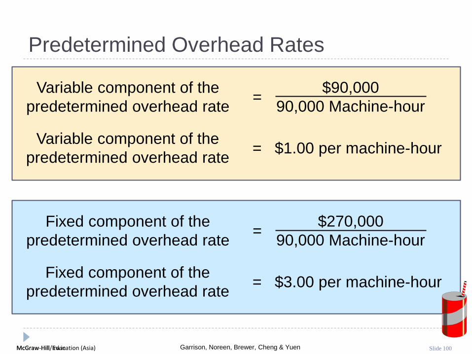
Predetermined Overhead Rates
Variable component of the
predetermined overhead rate
$90,000
90,000 Machine-hour=
Variable component of the
predetermined overhead rate= $1.00 per machine-hour
Fixed component of the
predetermined overhead rate
$270,000
90,000 Machine-hour=
Fixed component of the
predetermined overhead rate= $3.00 per machine-hour

McGraw-Hill Education (Asia) Garrison, Noreen, Brewer, Cheng & YuenMcGraw-Hill/Irwin Slide 101
Applying Manufacturing Overhead
Overhead
applied
Predetermined
overhead rate
Standard hours allowed
for the actual output= ×
Overhead
applied
$4.00 per
machine-hour84,000 machine-hour= ×
Overhead
applied$336,000=

McGraw-Hill Education (Asia) Garrison, Noreen, Brewer, Cheng & YuenMcGraw-Hill/Irwin Slide 102
Fixed Manufacturing Overhead Variances
Actual = = 280,000
10,000 U Budget variance
Budgeted = = 270,000
18,000 U Volume variance
SH x SR = (28000 x 3) x 3 = 252,000
28,000 U Total Underapplied overhead
SH = (Aouput x standard hours for the production)
= standard hours allowed for the actual output

McGraw-Hill Education (Asia) Garrison, Noreen, Brewer, Cheng & YuenMcGraw-Hill/Irwin Slide 103
Computing the Budget Variance
Budget
variance
Budgeted
fixed
overhead
Actual
fixed
overhead
= –
Budget
variance= $280,000 – $270,000
Budget
variance= $10,000 Unfavorable

McGraw-Hill Education (Asia) Garrison, Noreen, Brewer, Cheng & YuenMcGraw-Hill/Irwin Slide 104
Computing the Volume Variance
Volume
variance
Fixed
overhead
applied to
work in process
Budgeted
fixed
overhead
= –
Volume
variance= $18,000 Unfavorable
Volume
variance= $270,000 –
$3.00 per
machine-hour( ×$84,000
machine-hour)

McGraw-Hill Education (Asia) Garrison, Noreen, Brewer, Cheng & YuenMcGraw-Hill/Irwin Slide 105
Computing the Volume Variance
FPOHR = Fixed portion of the predetermined overhead rateDH = Denominator hoursSH = Standard hours allowed for actual output
Volume variance FPOHR × (DH – SH)=
Volume
variance=
$3.00 per
machine-hour (× 90,000
machine-hour
– 84,000
machine-hour)
Volume
variance= 18,000 Unfavorable

McGraw-Hill Education (Asia) Garrison, Noreen, Brewer, Cheng & YuenMcGraw-Hill/Irwin Slide 106
A Pictorial View of the Variances
Actual
Fixed
Overhead
Fixed Overhead
Applied to
Work in Process
Budgeted
Fixed
Overhead
252,000270,000280,000
Total variance, $28,000 unfavorable
Budget variance,
$10,000 unfavorable
Volume variance,
$18,000 unfavorable

McGraw-Hill Education (Asia) Garrison, Noreen, Brewer, Cheng & YuenMcGraw-Hill/Irwin Slide 107
Fixed Overhead Variances –A Graphic Approach
Let’s look at a
graph showing
fixed overhead
variances. We will
use ColaCo’s
numbers from the
previous example.

McGraw-Hill Education (Asia) Garrison, Noreen, Brewer, Cheng & YuenMcGraw-Hill/Irwin Slide 108
Graphic Analysis of FixedOverhead Variances
Machine-hours (000)
Budget
$270,000
90
Denominator
hours
0
0

McGraw-Hill Education (Asia) Garrison, Noreen, Brewer, Cheng & YuenMcGraw-Hill/Irwin Slide 109
Graphic Analysis of FixedOverhead Variances
Actual
$280,000
Machine-hours (000)
Budget
$270,000
90
Denominator
hours
0
0
Budget Variance 10,000 U{

McGraw-Hill Education (Asia) Garrison, Noreen, Brewer, Cheng & YuenMcGraw-Hill/Irwin Slide 110
Actual
$280,000
Applied
$252,000
Machine-hours (000)
Budget
$270,000
Graphic Analysis of FixedOverhead Variances
90840
0
Standard
hoursDenominator
hours
Budget Variance 10,000 U
Volume Variance 18,000 U
{{
McGraw-Hill Education (Asia) Garrison, Noreen, Brewer, Cheng & YuenMcGraw-Hill/Irwin Slide 111
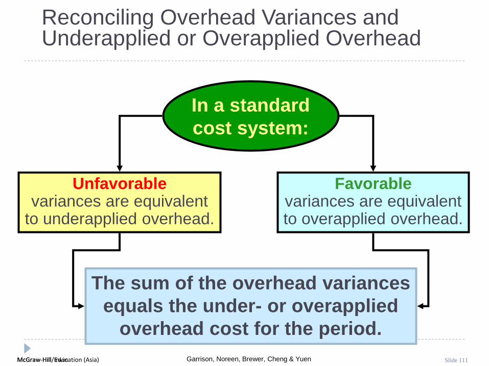
Reconciling Overhead Variances and Underapplied or Overapplied Overhead
In a standard
cost system:
Unfavorablevariances are equivalent
to underapplied overhead.
Favorablevariances are equivalentto overapplied overhead.
The sum of the overhead variances
equals the under- or overapplied
overhead cost for the period.

McGraw-Hill Education (Asia) Garrison, Noreen, Brewer, Cheng & YuenMcGraw-Hill/Irwin Slide 112
Reconciling Overhead Variances and Underapplied or Overapplied Overhead
Predetermined overhead rate (a) 4.00$ per machine-hour
Standard hours allowed for the actual output (b) 84,000 machine hours
Manufacturing overhead applied (a) × (b) 336,000$
Actual manufacturing overhead 380,000$
Manufacturing overhead underapplied or
overapplied 44,000$ underapplied
Computation of Underapplied Overhead
ColaCo
McGraw-Hill Education (Asia) Garrison, Noreen, Brewer, Cheng & YuenMcGraw-Hill/Irwin Slide 113
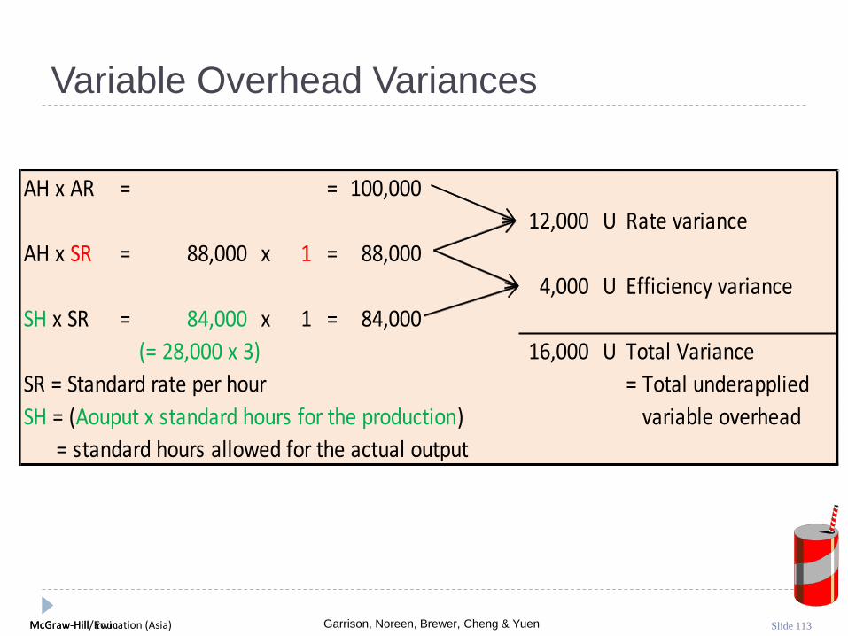
Variable Overhead Variances
AH x AR = = 100,000
12,000 U Rate variance
AH x SR = 88,000 x 1 = 88,000
4,000 U Efficiency variance
SH x SR = 84,000 x 1 = 84,000
(= 28,000 x 3) 16,000 U Total Variance
SR = Standard rate per hour = Total underapplied
SH = (Aouput x standard hours for the production) variable overhead
= standard hours allowed for the actual output

McGraw-Hill Education (Asia) Garrison, Noreen, Brewer, Cheng & YuenMcGraw-Hill/Irwin Slide 114
Computing the Variable Overhead Variances
Variable manufacturing overhead rate varianceVMRV = (AH × AR) – (AH × SR)
= $100,000 – (88,000 hours × $1.00 per hour)
= $12,000 unfavorable

McGraw-Hill Education (Asia) Garrison, Noreen, Brewer, Cheng & YuenMcGraw-Hill/Irwin Slide 115
Computing the Variable Overhead Variances
Variable manufacturing overhead efficiency varianceVMEV = (AH × SR) – (SH × SR)
= $88,000 – (84,000 hours × $1.00 per hour)
= $4,000 unfavorable

McGraw-Hill Education (Asia) Garrison, Noreen, Brewer, Cheng & YuenMcGraw-Hill/Irwin Slide 116
Computing the Sum of All Variances
Variable overhead rate variance 12,000$ U
Variable overhead efficiency variance 4,000 U
Fixed overhead budget variance 10,000 U
Fixed overhead volume variance 18,000 U
Total of the overhead variances 44,000$ U
Computing the Sum of All variances
ColaCo

© 2012 McGraw-Hill Education (Asia)Garrison, Noreen, Brewer, Cheng & Yuen
Journal Entries to Record
Variances
Appendix 12B

McGraw-Hill Education (Asia) Garrison, Noreen, Brewer, Cheng & YuenMcGraw-Hill/Irwin Slide 118
Learning Objective 7
(Appendix 12B)
Prepare journal entries
to record standard
costs and variances.

McGraw-Hill Education (Asia) Garrison, Noreen, Brewer, Cheng & YuenMcGraw-Hill/Irwin Slide 119
Appendix 12BJournal Entries to Record Variances
We will use information from the Glacier Peak Outfitters
example presented earlier in the chapter to illustrate journal
entries for standard cost variances. Recall the following:
Material
AQ × AP = $1,029
AQ × SP = $1,050
SQ × SP = $1,000
MPV = $21 F
MQV = $50 U
Labor
AH × AR = $26,250
AH × SR = $25,000
SH × SR = $24,000
LRV = $1,250 U
LEV = $1,000 U
Now, let’s prepare the entries to record
the labor and material variances.

McGraw-Hill Education (Asia) Garrison, Noreen, Brewer, Cheng & YuenMcGraw-Hill/Irwin Slide 120
GENERAL JOURNAL Page 4
Date Description
Post.
Ref. Debit Credit
Raw Materials 1,050
Materials Price Variance 21
Accounts Payable 1,029
To record the purchase of material
Work in Process 1,000
Materials Quantity Variance 50
Raw Materials 1,050
To record the use of material
Appendix 12BRecording Material Variances

McGraw-Hill Education (Asia) Garrison, Noreen, Brewer, Cheng & YuenMcGraw-Hill/Irwin Slide 121
GENERAL JOURNAL Page 4
Date Description
Post.
Ref. Debit Credit
Work in Process 24,000
Labor Rate Variance 1,250
Labor Efficiency Variance 1,000
Wages Payable 26,250
To record direct labor
Appendix 12BRecording Labor Variances

McGraw-Hill Education (Asia) Garrison, Noreen, Brewer, Cheng & YuenMcGraw-Hill/Irwin Slide 122
Cost Flows in a Standard Cost System
Inventories are recorded at standard cost.
Variances are recorded as follows:
Favorable variances are credits, representing
savings in production costs.
Unfavorable variances are debits, representing
excess production costs.
Standard cost variances are usually closed out
to cost of goods sold.
Unfavorable variances increase cost of goods sold.
Favorable variances decrease cost of goods sold.

McGraw-Hill Education (Asia) Garrison, Noreen, Brewer, Cheng & YuenMcGraw-Hill/Irwin Slide 123
End of Chapter 12