Debt Crises

For Whom the Bell Tolls

Harold Cole Daniel Neuhann Guillermo Ordonez

UPenn UPenn UPenn

September 3, 2016

1 / 37

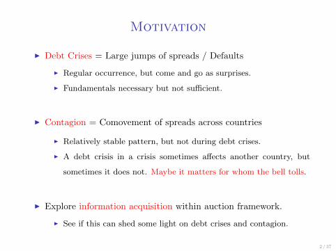
Motivation

I Debt Crises = Large jumps of spreads / Defaults

I Regular occurrence, but come and go as surprises.

I Fundamentals necessary but not sufficient.

I Contagion = Comovement of spreads across countries

I Relatively stable pattern, but not during debt crises.

I A debt crisis in a crisis sometimes affects another country, but

sometimes it does not. Maybe it matters for whom the bell tolls.

I Explore information acquisition within auction framework.

I See if this can shed some light on debt crises and contagion.

2 / 37

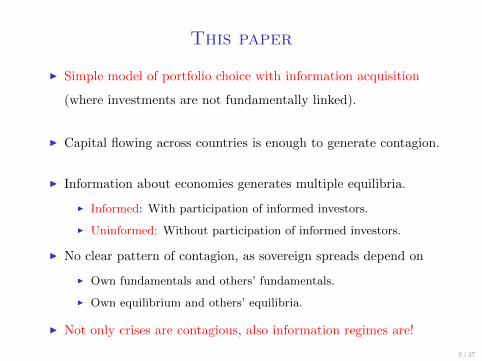
This paper

I Simple model of portfolio choice with information acquisition

(where investments are not fundamentally linked).

I Capital flowing across countries is enough to generate contagion.

I Information about economies generates multiple equilibria.

I Informed: With participation of informed investors.

I Uninformed: Without participation of informed investors.

I No clear pattern of contagion, as sovereign spreads depend on

I Own fundamentals and others’ fundamentals.

I Own equilibrium and others’ equilibria.

I Not only crises are contagious, also information regimes are!

3 / 37

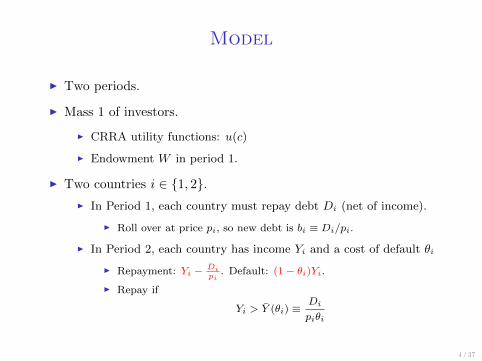
Model

I Two periods.

I Mass 1 of investors.

I CRRA utility functions: u(c)

I Endowment W in period 1.

I Two countries i ∈ {1, 2}.I In Period 1, each country must repay debt Di (net of income).

I Roll over at price pi, so new debt is bi ≡ Di/pi.

I In Period 2, each country has income Yi and a cost of default θi

I Repayment: Yi − Dipi

. Default: (1− θi)Yi.I Repay if

Yi > Y (θi) ≡Di

piθi

4 / 37

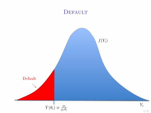
Default

5 / 37

f(Yi)

YiY (θi) ≡ Di

piθi

↘Default

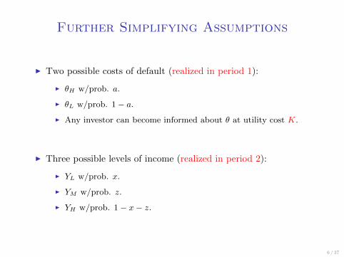
Further Simplifying Assumptions

I Two possible costs of default (realized in period 1):

I θH w/prob. a.

I θL w/prob. 1 − a.

I Any investor can become informed about θ at utility cost K.

I Three possible levels of income (realized in period 2):

I YL w/prob. x.

I YM w/prob. z.

I YH w/prob. 1 − x− z.

6 / 37

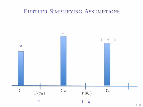
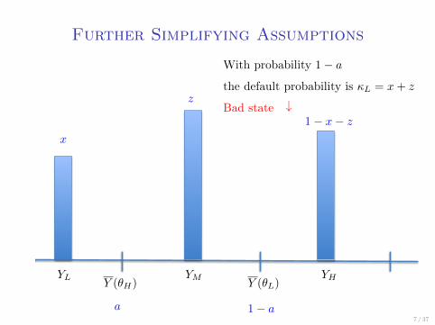
Further Simplifying Assumptions

7 / 37

YHYMYLY (θH) Y (θL)

1− x− z

z

x

a 1− a

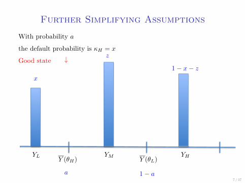
Further Simplifying Assumptions

7 / 37

YHYMYLY (θH) Y (θL)

1− x− z

z

x

a 1− a

With probability a

the default probability is κH = x

Good state ↓

Further Simplifying Assumptions

7 / 37

YHYMYLY (θH) Y (θL)

1− x− z

z

x

a 1− a

With probability 1− a

the default probability is κL = x+ z

Bad state ↓

Auctions

I In period 1 each country rolls over its debt using auctions

I Investors submit pair-orders (p, b).

I The country fills orders in decreasing order of p until it raises D.

I If there is a marginal price p, no reason to bid any other p.

Uninformed do not learn from prices before bidding, but they know

which are the possible prices in equilibrium after the bidding!

I No short-selling for commitment and information reasons (b ≥ 0).

8 / 37

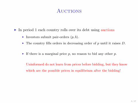
Auctions

I In period 1 each country rolls over its debt using auctions

I Investors submit pair-orders (p, b).

I The country fills orders in decreasing order of p until it raises D.

I If there is a marginal price p, no reason to bid any other p.

Uninformed do not learn from prices before bidding, but they know

which are the possible prices in equilibrium after the bidding!

I No short-selling for commitment and information reasons (b ≥ 0).

8 / 37

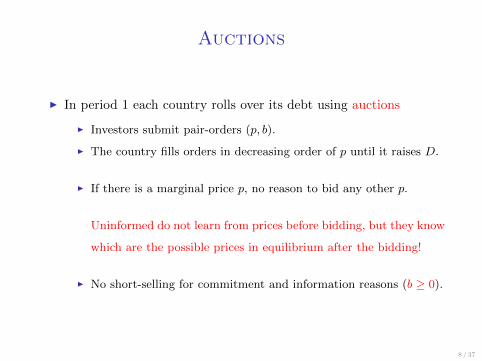
A Single Country

9 / 37

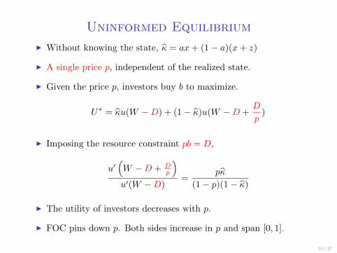
Uninformed Equilibrium

10 / 37

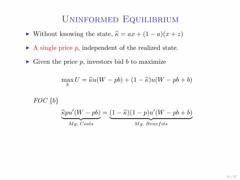
I Without knowing the state, κ = ax+ (1− a)(x+ z)

I A single price p, independent of the realized state.

I Given the price p, investors bid b to maximize

maxbU = κu(W − pb) + (1− κ)u(W − pb+ b)

FOC {b}

κpu′(W − pb)︸ ︷︷ ︸Mg. Costs

= (1− κ)(1− p)u′(W − pb+ b)︸ ︷︷ ︸Mg. Benefits

Uninformed Equilibrium

10 / 37

I Without knowing the state, κ = ax+ (1− a)(x+ z)

I A single price p, independent of the realized state.

I Given the price p, investors bid b to maximize

maxbU = κu(W − pb) + (1− κ)u(W − pb+ b)

FOC {b}

u′(W − pb+ b)

u′(W − pb)=

pκ

(1− p)(1− κ)=⇒ b( p

(−), κ(−)

)

I If p = 1− κ, then b = 0. Investors charge a risk premium!

Uninformed Equilibrium

10 / 37

I Without knowing the state, κ = ax+ (1− a)(x+ z)

I A single price p, independent of the realized state.

I Given the price p, investors buy b to maximize.

U∗ = κu(W −D) + (1− κ)u(W −D +D

p)

I Imposing the resource constraint pb = D,

u′(W −D + D

p

)u′(W −D)

=pκ

(1− p)(1− κ)

I The utility of investors decreases with p.

I FOC pins down p. Both sides increase in p and span [0, 1].

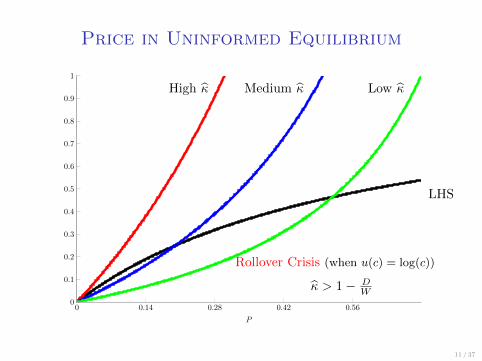
Price in Uninformed Equilibrium

0 0.14 0.28 0.42 0.560

0.1

0.2

0.3

0.4

0.5

0.6

0.7

0.8

0.9

1

P

11 / 37

High κ Medium κ Low κ

LHS

Rollover Crisis (when u(c) = log(c))

κ > 1− DW

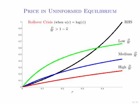
Price in Uninformed Equilibrium

0 0.1 0.2 0.3 0.40

0.1

0.2

0.3

0.4

0.5

0.6

0.7

0.8

0.9

1

P

12 / 37

Low DW

Medium DW

High DW

RHSRollover Crisis (when u(c) = log(c))

DW > 1− κ

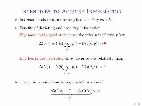
Incentives to Acquire Information

13 / 37

I Information about θ can be acquired at utility cost K.

Incentives to Acquire Information

13 / 37

I Information about θ can be acquired at utility cost K.

I Benefits of deviating and acquiring information:

Buy more in the good state, since the price p is relatively low.

∆(UH) ≡ U(b( κH︸︷︷︸x

, p))− U(b(κ, p)) > 0

Buy less in the bad state, since the price p is relatively high.

∆(UL) ≡ U(b( κL︸︷︷︸x+z

, p))− U(b(κ, p)) > 0

I There are no incentives to acquire information if

a∆(UH) + (1− a)∆(UL)︸ ︷︷ ︸χU

< K

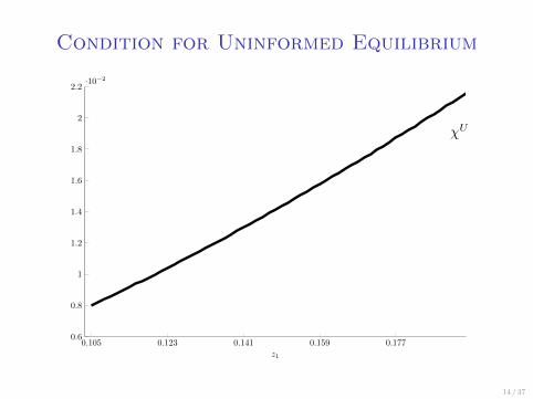
Condition for Uninformed Equilibrium

0.105 0.123 0.141 0.159 0.1770.6

0.8

1

1.2

1.4

1.6

1.8

2

2.2·10−2

z1

14 / 37

χU

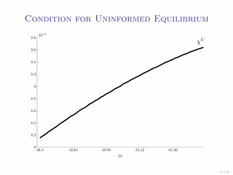
Condition for Uninformed Equilibrium

36.4 42.64 48.88 55.12 61.368

8.2

8.4

8.6

8.8

9

9.2

9.4

9.6

9.8·10−3

D1

15 / 37

χU

Informed Investors

16 / 37

I Informed investors know the state, κH = x and κL = x+ z

I Same maximization as before, but knowing the state s ∈ {L,H}.

Then

u′(W − psbIs + bIs)

u′(W − psbIs)=

psκs(1− ps)(1− κs)

=⇒ bIs( ps(−), κs(−)

)

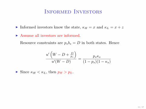
Informed Investors

16 / 37

I Informed investors know the state, κH = x and κL = x+ z

I Assume all investors are informed.

Resource constraints are psbs = D in both states. Hence

u′(W −D + D

ps

)u′(W −D)

=psκs

(1− ps)(1− κs)

I Since κH < κL, then pH > pL.

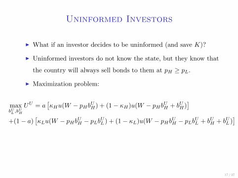
Uninformed Investors

17 / 37

I What if an investor decides to be uninformed (and save K)?

I Uninformed investors do not know the state, but they know that

the country will always sell bonds to them at pH ≥ pL.

I Maximization problem:

maxbUL ,b

UH

UU = a[κHu(W − pHbUH) + (1− κH)u(W − pHbUH + bUH)

]+(1− a)

[κLu(W − pHbUH − pLbUL ) + (1− κL)u(W − pHbUH − pLbUL + bUH + bUL )

]

Uninformed Investors

17 / 37

I FOC {bUH} They always get to buy at pH .

a[pHκHu′(W−pHbUH)] +(1−a)[pHκLu

′(W−pHbUH−pLbUL )]

= a[(1−pH)(1−κH)u′(W−pHbUH+bUH)]+(1−a)[(1−pH)(1−κL)u′(W−pHbUH−pLbUL+bUH+bUL )]

I FOC {bUL}When they get to buy at pL, they also buy part at pH .

pLκLu′(W−pHbUH−pLb

UL ) = (1−pL)(1−κL)u′(W−pHbUH−pLb

UL+bUH+bUL )

Uninformed Investors

17 / 37

I FOC {bUH} They always get to buy at pH .

a[pHκHu′(W−pHbUH)] +(1−a)[pHκLu

′(W−pHbUH−pLbUL )]

= a[(1−pH)(1−κH)u′(W−pHbUH+bUH)]+(1−a)[(1−pH)(1−κL)u′(W−pHbUH−pLbUL+bUH+bUL )]

I FOC {bUL}When they get to buy at pL, they also buy part at pH .

pLκLu′(W−pHbUH−pLb

UL ) = (1−pL)(1−κL)u′(W−pHbUH−pLb

UL+bUH+bUL )

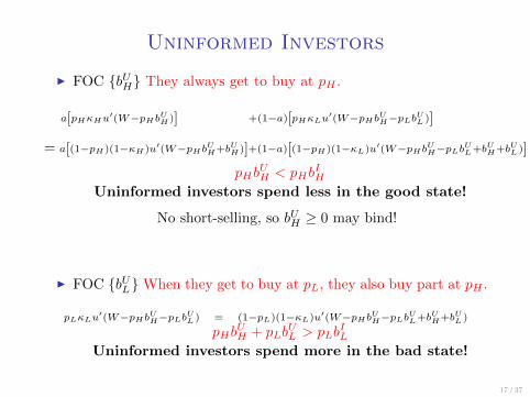
pHbUH + pLb

UL > pLb

IL

Uninformed investors spend more in the bad state!

pHbUH < pHb

IH

Uninformed investors spend less in the good state!

No short-selling, so bUH ≥ 0 may bind!

Resource Constraints

18 / 37

Denote by n the fraction of informed investors.

npHbIH + (1− n)pHb

UH = D

npLbIL + (1− n)[pHb

UH + pLb

UL ] = D

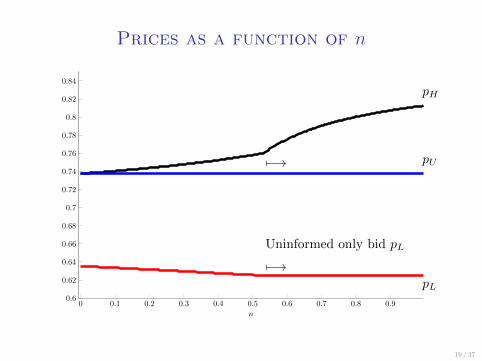
Prices as a function of n

0 0.1 0.2 0.3 0.4 0.5 0.6 0.7 0.8 0.90.6

0.62

0.64

0.66

0.68

0.7

0.72

0.74

0.76

0.78

0.8

0.82

0.84

n

19 / 37

7−→

7−→

Uninformed only bid pL

pH

pL

pU

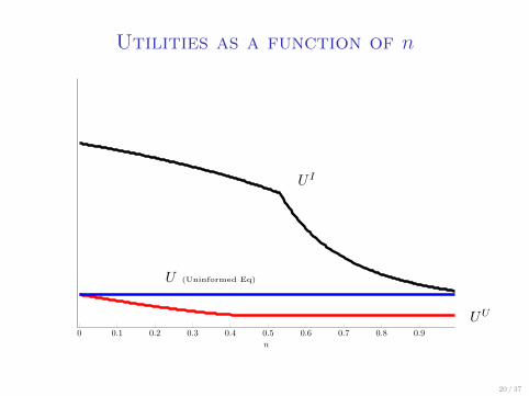
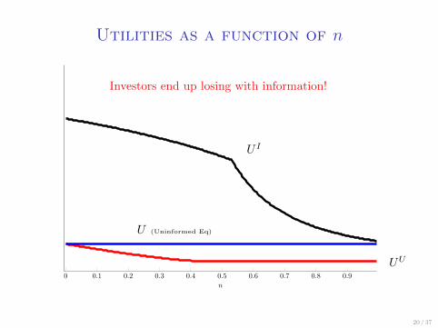
Utilities as a function of n

0 0.1 0.2 0.3 0.4 0.5 0.6 0.7 0.8 0.9

n

20 / 37

U I

UU

U (Uninformed Eq)

Utilities as a function of n

0 0.1 0.2 0.3 0.4 0.5 0.6 0.7 0.8 0.9

n

20 / 37

U I

UU

U (Uninformed Eq)

Investors end up losing with information!

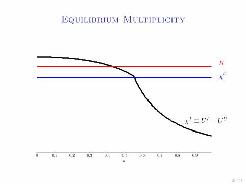
Equilibrium Multiplicity

0 0.1 0.2 0.3 0.4 0.5 0.6 0.7 0.8 0.9

n

21 / 37

χI ≡ U I − UU

χU

K

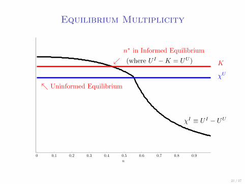
Equilibrium Multiplicity

0 0.1 0.2 0.3 0.4 0.5 0.6 0.7 0.8 0.9

n

21 / 37

χI ≡ U I − UU

χU

K

↖ Uninformed Equilibrium

n∗ in Informed Equilibrium

↙ (where U I −K = UU )

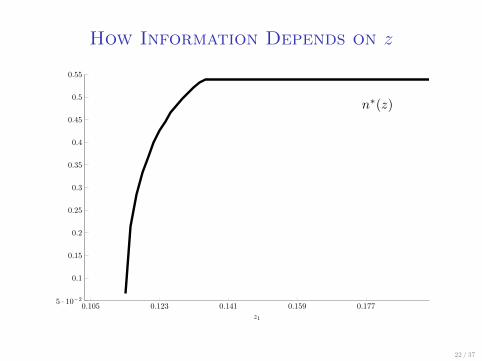
How Information Depends on z

0.105 0.123 0.141 0.159 0.1775 · 10−2

0.1

0.15

0.2

0.25

0.3

0.35

0.4

0.45

0.5

0.55

z1

22 / 37

n∗(z)

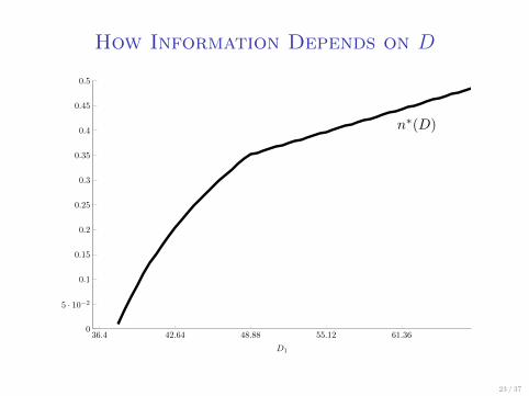
How Information Depends on D

36.4 42.64 48.88 55.12 61.360

5 · 10−2

0.1

0.15

0.2

0.25

0.3

0.35

0.4

0.45

0.5

D1

23 / 37

n∗(D)

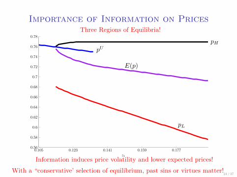
Importance of Information on Prices

0.105 0.123 0.141 0.159 0.1770.56

0.58

0.6

0.62

0.64

0.66

0.68

0.7

0.72

0.74

0.76

0.78

z1

24 / 37

pH

pL

pU

E(p)

Three Regions of Equilibria!

Information induces price volatility and lower expected prices!

With a “conservative’ selection of equilibrium, past sins or virtues matter!

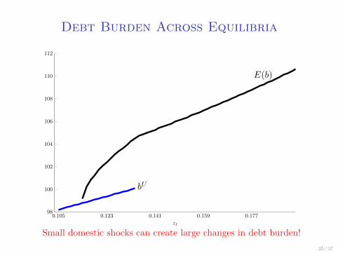
Debt Burden Across Equilibria

0.105 0.123 0.141 0.159 0.17798

100

102

104

106

108

110

112

z1

25 / 37

bU

E(b)

Small domestic shocks can create large changes in debt burden!

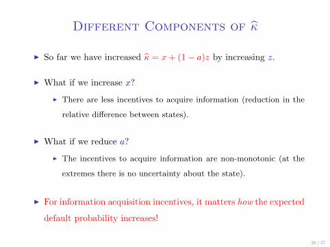
Different Components of κ

I So far we have increased κ = x+ (1− a)z by increasing z.

I What if we increase x?

I There are less incentives to acquire information (reduction in the

relative difference between states).

I What if we reduce a?

I The incentives to acquire information are non-monotonic (at the

extremes there is no uncertainty about the state).

I For information acquisition incentives, it matters how the expected

default probability increases!

26 / 37

Two Countries

27 / 37

Two Country Model

28 / 37

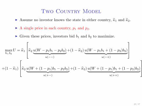
I Assume no investor knows the state in either country, κ1 and κ2.

I A single price in each country, p1 and p2.

I Given these prices, investors bid b1 and b2 to maximize.

maxb1,b2

U = κ1

κ2 u(W − p1b1 − p2b2)︸ ︷︷ ︸u(−−)

+(1− κ2)u(W − p1b1 + (1− p2)b2)︸ ︷︷ ︸u(−+)

+(1− κ1)

κ2 u(W + (1− p1)b1 − p2b2)︸ ︷︷ ︸u(+−)

+(1− κ2)u(W + (1− p1)b1 + (1− p2)b2)︸ ︷︷ ︸u(++)

Symmetric Simple Setting

I To hold # of prices and bids we assume that investors

1. Allocate funds between country 1 and 2.

2. Choose whether to become informed in country 1 or 2 or both.

3. Bid in each country.

I We also assume countries are completely symmetric

I Only 2 prices: pH and pL.

I Only 4 bids: biH and biL (conditional on θi only if informed).

29 / 37

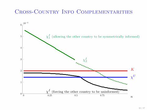
Cross-Country Info Complementarities

0 0.25 0.5 0.750

1

2

3

4

5

6·10−2

30 / 37

χI (forcing the other country to be uninformed)

χI1 (allowing the other country to be symmetrically informed)

χI2

χU

K

n

Cross-Country Info Complementarities

0 0.25 0.5 0.750

1

2

3

4

5

6·10−2

30 / 37

χI2

χU

K

n

χI

χI1

If the other country is uninformed

Only uninformed equilibrium is feasible!

If the other country is symmetrically informed

Uninformed and “very” informed equilibrium coexist!

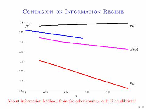
Contagion on Information Regime

0.1 0.13 0.16 0.19 0.220.45

0.5

0.55

0.6

0.65

0.7

0.75

0.8

z1

32 / 37

pU pH

pL

E(p)

Absent information feedback from the other country, only U equilibrium!

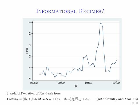
Informational Regimes?

31 / 37

.51

1.5

22.5

3sdres

2000q1 2005q1 2010q1 2015q1tq

Standard Deviation of Residuals from

Y ieldsit = (β1 + β2Ic)∆GDPit + (β3 + β4Ic) DebtGDP it

+ εit (with Country and Year FE)

Contagion on Information Regime

0.1 0.13 0.16 0.19 0.220.45

0.5

0.55

0.6

0.65

0.7

0.75

0.8

z1

32 / 37

pU pH

pL

E(p)

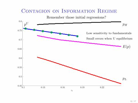
Remember those initial regressions?

•••••••Low sensitivity to fundamentals

Small errors when U equilibrium

Contagion on Information Regime

0.1 0.13 0.16 0.19 0.220.45

0.5

0.55

0.6

0.65

0.7

0.75

0.8

z1

32 / 37

pU pH

pL

E(p)

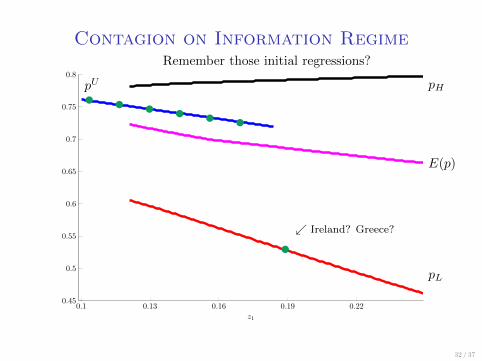
Remember those initial regressions?

••••••

•↙ Ireland? Greece?

Contagion on Information Regime

0.1 0.13 0.16 0.19 0.220.45

0.5

0.55

0.6

0.65

0.7

0.75

0.8

z1

32 / 37

pU pH

pL

E(p)

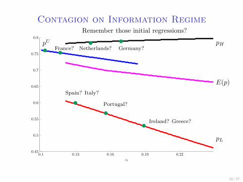
Remember those initial regressions?

••

•

•

•

•

•

Ireland? Greece?

Germany?Netherlands?France?

Portugal?

Spain? Italy?

Contagion on Information Regime

0.1 0.13 0.16 0.19 0.220.45

0.5

0.55

0.6

0.65

0.7

0.75

0.8

z1

32 / 37

pU pH

pL

E(p)

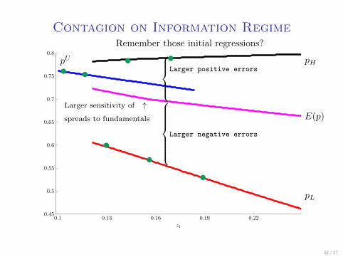
Remember those initial regressions?

••

•

•

•

•

•

Larger sensitivity of ↑

spreads to fundamentals

Larger positive errors

Larger negative errors

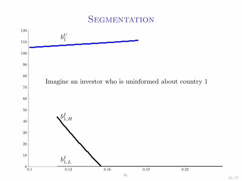
Segmentation

0.1 0.13 0.16 0.19 0.220

10

20

30

40

50

60

70

80

90

100

110

120

z133 / 37

Imagine an investor who is uninformed about country 1

bU1

bI1,H

bI1,L

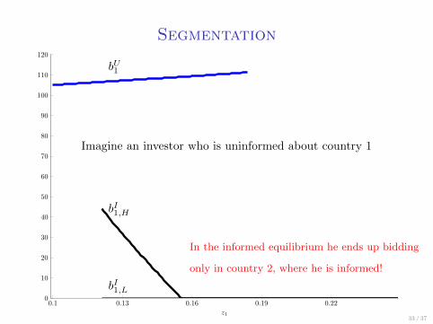
Segmentation

0.1 0.13 0.16 0.19 0.220

10

20

30

40

50

60

70

80

90

100

110

120

z133 / 37

Imagine an investor who is uninformed about country 1

bU1

bI1,H

bI1,L

In the informed equilibrium he ends up bidding

only in country 2, where he is informed!

Magnification of Contagion

I So far we have discussed contagion in its purest form, but there

are magnifying forces.

I Endogenous probability of default (κi depends on pi).

I Fundamental linkages (κi depends on κ−i).

I Time-varying prudence (risk-aversion that changes with wealth).

I Market segmentation concentrates contagion.

I Structure of information costs across countries.

34 / 37

Suggestive Thoughts

I How can Japan or the U.S. sustain very large debt/GDP ratios

with low and stable spreads?

Uninformed Equilibrium?

I Why can many countries not raise their debt/GDP ratio without

triggering high volatility and increases in spreads?

Informed Equilibrium?

35 / 37

Extensions

I Extension to K states and I countries.

I Just add FOCs and resource constraints.

I Extension to a continuous distribution of Y .

I Thresholds Y (θk) are endogenous and jointly determined with the

probability of default in each state.

36 / 37

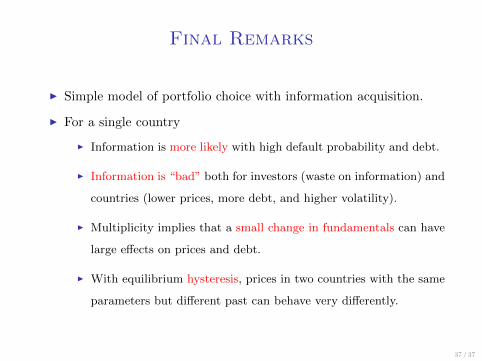
Final Remarks

I Simple model of portfolio choice with information acquisition.

I For a single country

I Information is more likely with high default probability and debt.

I Information is “bad” both for investors (waste on information) and

countries (lower prices, more debt, and higher volatility).

I Multiplicity implies that a small change in fundamentals can have

large effects on prices and debt.

I With equilibrium hysteresis, prices in two countries with the same

parameters but different past can behave very differently.

37 / 37

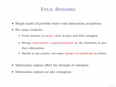
Final Remarks

I Simple model of portfolio choice with information acquisition.

I For many countries

I Given investor prudence, there is price and debt contagion.

I Strong cross-country complementarities on the incentives to pro-

duce information.

I Shocks in one country can cause changes of equilibrium in others.

I Information regimes affect the strength of contagion.

I Information regimes are also contagious.

37 / 37

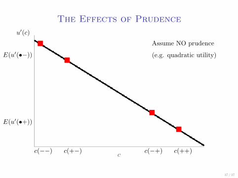
The Effects of Prudence

C

37 / 37

Assume NO prudence

(e.g. quadratic utility)

u′(c)

c(−−) c(+−) c(−+) c(++)

�

�

�

�

E(u′(•−))

E(u′(•+))

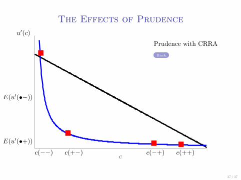
The Effects of Prudence

C

37 / 37

Prudence with CRRA

Back

u′(c)

c(−−) c(+−) c(−+) c(++)

�

�� �

E(u′(•−))

E(u′(•+))