Embed Size (px)
Citation preview
Bayesian Graphical Models for Structural VectorAutoregressive Processes
SYstemic Risk TOmography:Signals, Measurements, Transmission Channels, and Policy Interventions
D. F. Ahelegbey, Ca’ Foscari University of Venice (Italy)M. Billio, Ca’ Foscari University of Venice (Italy)R. Casarin, Ca' Foscari University of Venice (Italy)
ENSAE. November 21, 2013.
Bayesian Graphical Models for Structural VectorAutoregressive Processes
Daniel Felix Ahelegbey, Monica Billio, Roberto Casarin
Department of Economics, Ca’ Foscari University of Venice, Italy
Networks in Economics and Finance,ENSAE-Paris Tech, November 18 - 22, 2013
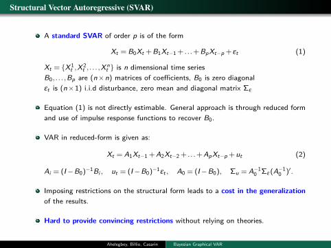
Structural Vector Autoregressive (SVAR)
A standard SVAR of order p is of the form
Xt = B0Xt + B1Xt−1 + . . .+ BpXt−p + εt (1)
Xt = X1t ,X2
t , . . . ,Xnt is n dimensional time series
B0, . . . ,Bp are (n×n) matrices of coefficients, B0 is zero diagonalεt is (n×1) i.i.d disturbance, zero mean and diagonal matrix Σε
Equation (1) is not directly estimable. General approach is through reduced formand use of impulse response functions to recover B0.
VAR in reduced-form is given as:
Xt = A1Xt−1 + A2Xt−2 + . . .+ ApXt−p + ut (2)
Ai = (I−B0)−1Bi , ut = (I−B0)−1εt , A0 = (I−B0), Σu = A−10 Σε (A−1
0 )′.
Imposing restrictions on the structural form leads to a cost in the generalizationof the results.
Hard to provide convincing restrictions without relying on theories.
Ahelegbey, Billio, Casarin Bayesian Graphical VAR
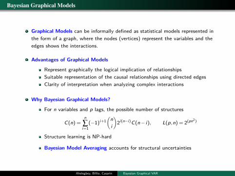
Bayesian Graphical Models
Graphical Models can be informally defined as statistical models represented inthe form of a graph, where the nodes (vertices) represent the variables and theedges shows the interactions.
Advantages of Graphical Models
Represent graphically the logical implication of relationshipsSuitable representation of the causal relationships using directed edgesClarity of interpretation when analyzing complex interactions
Why Bayesian Graphical Models?
For n variables and p lags, the possible number of structures
C(n) =n∑i=1
(−1)i+1(
ni
)2i(n−i)C(n− i), L(p,n) = 2(pn2)
Structure learning is NP-hard
Bayesian Model Averaging accounts for structural uncertainties
Ahelegbey, Billio, Casarin Bayesian Graphical VAR
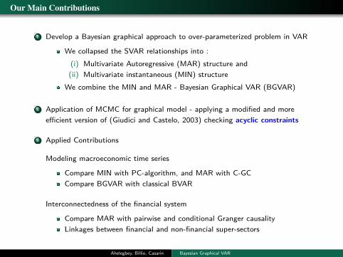
Our Main Contributions
1 Develop a Bayesian graphical approach to over-parameterized problem in VAR
We collapsed the SVAR relationships into :(i) Multivariate Autoregressive (MAR) structure and(ii) Multivariate instantaneous (MIN) structure
We combine the MIN and MAR - Bayesian Graphical VAR (BGVAR)
2 Application of MCMC for graphical model - applying a modified and moreefficient version of (Giudici and Castelo, 2003) checking acyclic constraints
3 Applied Contributions
Modeling macroeconomic time series
Compare MIN with PC-algorithm, and MAR with C-GCCompare BGVAR with classical BVAR
Interconnectedness of the financial system
Compare MAR with pairwise and conditional Granger causalityLinkages between financial and non-financial super-sectors
Ahelegbey, Billio, Casarin Bayesian Graphical VAR
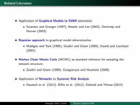
Related Literature
Application of Graphical Models to SVAR estimation
Swanson and Granger (1997), Bessler and Lee (2002), Demiralp andHoover (2003)
Bayesian approach to graphical model determination
Madigan and York (1995), Giudici and Green (1999), Dawid and Lauritzen(2001)
Markov Chain Monte Carlo (MCMC) as standard inference for sampling thenetwork structure
Giudici and Green (1999), Grzegorczyk and Husmeier (2008)
Application of Networks to Systemic Risk Analysis
Hautsch et al. (2012), Billio et al. (2012), Diebold and Yilmaz (2013)
Ahelegbey, Billio, Casarin Bayesian Graphical VAR
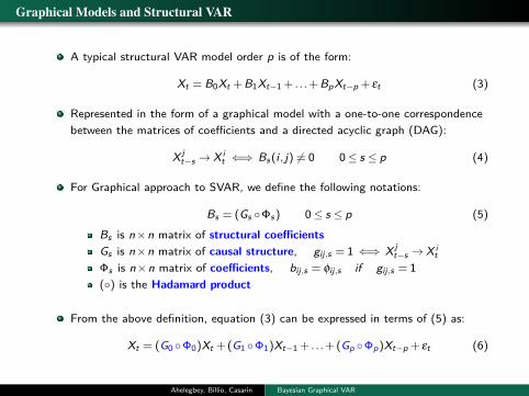
Graphical Models and Structural VAR
A typical structural VAR model order p is of the form:
Xt = B0Xt + B1Xt−1 + . . .+ BpXt−p + εt (3)
Represented in the form of a graphical model with a one-to-one correspondencebetween the matrices of coefficients and a directed acyclic graph (DAG):
X jt−s → X i
t ⇐⇒ Bs (i , j) 6= 0 0≤ s ≤ p (4)
For Graphical approach to SVAR, we define the following notations:
Bs = (Gs Φs ) 0≤ s ≤ p (5)
Bs is n×n matrix of structural coefficientsGs is n×n matrix of causal structure, gij,s = 1 ⇐⇒ X j
t−s → X it
Φs is n×n matrix of coefficients, bij,s = φij,s if gij,s = 1() is the Hadamard product
From the above definition, equation (3) can be expressed in terms of (5) as:
Xt = (G0 Φ0)Xt + (G1 Φ1)Xt−1 + . . .+ (Gp Φp)Xt−p + εt (6)
Ahelegbey, Billio, Casarin Bayesian Graphical VAR

Efficient Inference Scheme
We assume the marginal prior distribution on gij is a Bernoulli, therefore we havea uniform prior over all DAGs
Following (Geiger and Heckerman, 1994), we assume parameter independenceand modularity. This allows for marginalizing out the parameters to estimate thedependence structure.
Assume variables are samples from a multivariate normal distribution
Assume normal-Wishart prior (Geiger and Heckerman, 1994)
Score DAGs with Bayesian Gaussian equivalent (BGe) metric.
Search involves Addition or Removal of an edge at each iteration
Modify the proposal by (Giudici and Castelo, 2003) for acyclic constraints incontemporaneous dependence
Use the standard acceptance and rejection criterion for MCMC
Ahelegbey, Billio, Casarin Bayesian Graphical VAR
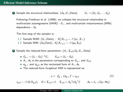
Efficient Model Inference Scheme
1 Sample the structural relationships: (G0,G+|Data), G+ = (G1,G2, . . . ,Gp)
Following Friedman et al. (1998), we collapse the structural relationship inmultivariate autoregressive (MAR) - G+, and multivariate instantaneous (MIN)dependence - G0
The first step of the sampler is:
1.1 Sample MAR: (G+|Data), : X it |Xt−p ∼N (µ+,Σ+)
1.2 Sample MIN: (G0|Data), : X it |Xt\i ∼N (µ0,Σ0)
2 Sample the reduced-form parameters: (A+,Σa,0|G0,G+,Data)
Ga,+ = (In−G0)−1G+ Ga,0 = (In−G0)
A+,A0 is the parameters corresponding to Ga,+ and Ga,0αg ,+ and αg ,0 as the vectorized form of A+,A0The reduced-form Graphical VAR is represented as:
y = Zg ,+ (αg ,+)′+ vg ,0 (7)
vg ,0 ∼N (0,Ωg ,0), Ω = Σa,0⊗ I, Σa,0 = A−10 (A−1
0 )′ A0 = In− (G0 Φ0)
Ahelegbey, Billio, Casarin Bayesian Graphical VAR
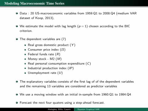
Modeling Macroeconomic Time Series
Data : 20 US-macroeconomic variables from 1959:Q1 to 2008:Q4 (medium VARdataset of Koop, 2013),
We estimate the model with lag length (p = 1) chosen according to the BICcriterion.
The dependent variables are (7)
Real gross domestic product (Y )Consumer price index (Π)Federal funds rate (R)Money stock - M2 (M)Real personal consumption expenditure (C)Industrial production index (IP)Unemployment rate (U)
The explanatory variables consists of the first lag of of the dependent variablesand the remaining 13 variables are considered as predictor variables
We use a moving window with an initial in-sample from 1960:Q1 to 1984:Q4
Forecast the next four quaters using a step-ahead forecast.
Ahelegbey, Billio, Casarin Bayesian Graphical VAR
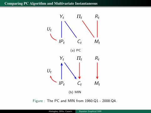
Comparing PC Algorithm and Multivariate Instantaneous
Ut
IPt
Yt Πt Rt
Ct Mt
(a) PC
Ut
IPt
Yt Πt Rt
Ct Mt
(b) MIN
Figure : The PC and MIN from 1960:Q1 - 2008:Q4.
Ahelegbey, Billio, Casarin Bayesian Graphical VAR
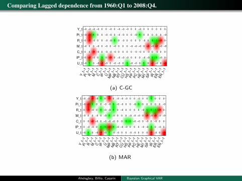
Comparing Lagged dependence from 1960:Q1 to 2008:Q4.
−0
−0
0
−0
0
0
−0
−0
−1
−1
0
0
−1
1
−0
1
−0
0
−1
−0
0
−0
0
0
−0
−0
0
−0
0
0
0
0
0
1
−1
0
−0
−0
−0
−0
0
−0
−0
−0
−0
0
−0
−1
0
0
0
1
−0
−0
0
−0
−0
−0
0
0
0
−0
−0
−0
−0
−0
0
0
−0
0
−0
0
0
0
0
−0
1
0
0
0
−0
0
0
−0
0
−0
0
−0
−0
0
−0
−0
1
0
−0
−0
0
0
0
0
−0
0
0
−0
1
0
0
0
−1
−0
−0
0
0
0
1
−0
0
1
−1
0
0
1
−1
−0
1
−0
0
0
−1
−0
0
−0
0
0
−0
0
−0
0
0
−1
Y_t−
1P
i_t−
1R
_t−
1M
_t−
1C
_t−
1IP
_t−
1U
_t−
1M
P_t−
1N
B_t−
1R
T_t−
1C
U_t−
1H
S_t−
1P
P_t−
1P
C_t−
1H
E_t−
1M
1_t−
1S
P_t−
1IR
_t−
1E
R_t−
1E
N_t−
1
Y_t
Pi_t
R_t
M_t
C_t
IP_t
U_t
(a) C-GC
−0
−0
0
−0
0
0
−0
−0
−1
−1
0
0
−0
1
−1
1
−0
0
−1
−0
0
−0
0
0
−0
−0
0
−0
1
0
1
0
0
1
−1
0
−0
−0
−0
−0
1
−0
−1
−0
−0
1
−0
−1
1
0
1
1
−0
−0
1
−0
−0
−0
0
0
0
−0
−0
−0
−0
−0
0
0
−0
0
−0
0
0
0
1
−0
0
0
0
0
−0
1
0
−0
0
−0
0
−0
−0
0
−0
−0
1
0
−0
−0
0
0
0
0
−0
0
0
−0
0
0
0
1
−1
−0
−0
0
1
0
1
−0
0
1
−1
0
0
1
−1
−0
0
−0
0
0
−1
−0
0
−0
0
0
−0
0
−0
0
0
−1
Y_t−
1P
i_t−
1R
_t−
1M
_t−
1C
_t−
1IP
_t−
1U
_t−
1M
P_t−
1N
B_t−
1R
T_t−
1C
U_t−
1H
S_t−
1P
P_t−
1P
C_t−
1H
E_t−
1M
1_t−
1S
P_t−
1IR
_t−
1E
R_t−
1E
N_t−
1
Y_t
Pi_t
R_t
M_t
C_t
IP_t
U_t
(b) MAR
Ahelegbey, Billio, Casarin Bayesian Graphical VAR
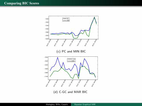
Comparing BIC Scores
−1620
−1600
−1580
−1560
−1540
−1520
−1500
60:Q
1−84:Q
4
64:Q
1−88:Q
4
68:Q
1−92:Q
4
72:Q
1−96:Q
4
76:Q
1−00:Q
4
80:Q
1−04:Q
4
84:Q
1−08:Q
4
PC
MIN
(c) PC and MIN BIC
−1700
−1680
−1660
−1640
−1620
−1600
60:Q
1−84:Q
4
64:Q
1−88:Q
4
68:Q
1−92:Q
4
72:Q
1−96:Q
4
76:Q
1−00:Q
4
80:Q
1−04:Q
4
84:Q
1−08:Q
4
C−GC
MAR
(d) C-GC and MAR BIC
Ahelegbey, Billio, Casarin Bayesian Graphical VAR
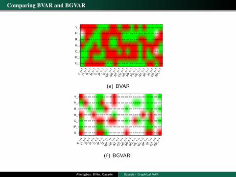
Comparing BVAR and BGVAR
−0.15
0.00
0.07
−0.27
0.07
0.08
0.02
−0.10
−0.80
−0.34
0.34
0.18
0.32
−0.10
−0.01
−0.03
0.32
0.15
−0.12
−0.03
−0.08
−0.06
0.01
0.18
−0.29
−0.20
0.19
−0.19
0.32
0.11
0.22
0.11
−0.11
0.32
−0.19
0.20
−0.14
−0.02
−0.08
0.03
0.43
−0.23
0.19
−0.34
−0.19
−0.01
−0.13
−0.23
0.07
−0.05
−0.06
0.06
0.23
−0.19
−0.14
0.11
−0.22
−0.31
0.05
0.34
−0.03
−0.12
−0.06
0.40
−0.38
−0.17
−0.11
0.29
−0.03
0.01
−0.33
0.17
0.08
−0.02
−0.07
−0.06
0.28
−0.03
0.11
0.08
−0.19
0.27
−0.08
0.01
0.16
0.04
0.24
−0.42
−0.04
−0.16
0.08
−0.06
0.61
0.06
−0.03
−0.36
−0.17
0.09
0.02
0.09
−0.04
0.01
0.21
0.07
0.03
−0.09
0.05
−0.08
−0.16
−0.01
−0.07
0.15
0.24
0.05
0.11
−0.20
0.16
0.27
−0.14
0.02
0.12
0.37
−0.48
−0.14
0.23
−0.12
0.05
0.00
−0.08
−0.05
0.00
−0.12
0.11
0.62
−0.29
−0.11
0.28
0.37
−0.12
−0.50
Y_t−
1P
i_t−
1R
_t−
1M
_t−
1C
_t−
1IP
_t−
1U
_t−
1M
P_t−
1N
B_t−
1R
T_t−
1C
U_t−
1H
S_t−
1P
P_t−
1P
C_t−
1H
E_t−
1M
1_t−
1S
P_t−
1IR
_t−
1E
R_t−
1E
N_t−
1
Y_t
Pi_t
R_t
M_t
C_t
IP_t
U_t
(e) BVAR
−0.08
0.03
−0.00
−0.19
0.16
0.19
−0.06
0.00
−0.78
0.00
0.00
0.00
0.00
0.00
0.00
0.00
0.37
0.00
0.00
0.00
0.00
0.00
0.00
0.00
−0.07
0.00
0.00
0.00
0.27
0.06
0.25
0.00
−0.21
0.21
−0.11
0.05
−0.05
0.04
0.00
−0.03
0.34
−0.14
0.00
0.00
−0.19
0.00
0.00
0.00
0.07
0.00
0.00
0.00
0.00
−0.12
0.00
0.00
−0.22
−0.46
0.00
0.03
−0.08
0.00
0.00
0.00
0.00
0.00
0.00
0.00
0.00
0.00
0.00
0.00
0.00
0.00
0.00
0.00
0.00
0.00
0.00
0.08
0.00
0.19
0.00
−0.16
0.00
0.00
0.00
0.00
0.00
0.00
0.00
0.00
0.63
0.00
0.00
−0.23
0.00
0.00
0.00
0.08
0.00
0.00
0.16
0.00
0.00
0.00
0.00
0.00
−0.30
0.00
0.00
0.00
0.18
0.05
0.04
0.00
0.19
0.21
−0.04
0.05
0.10
0.24
−0.31
−0.09
0.15
−0.06
0.00
0.00
0.00
0.00
0.00
0.00
0.00
0.24
0.00
0.02
0.00
0.26
0.00
−0.39
Y_t−
1P
i_t−
1R
_t−
1M
_t−
1C
_t−
1IP
_t−
1U
_t−
1M
P_t−
1N
B_t−
1R
T_t−
1C
U_t−
1H
S_t−
1P
P_t−
1P
C_t−
1H
E_t−
1M
1_t−
1S
P_t−
1IR
_t−
1E
R_t−
1E
N_t−
1
Y_t
Pi_t
R_t
M_t
C_t
IP_t
U_t
(f) BGVAR
Ahelegbey, Billio, Casarin Bayesian Graphical VAR
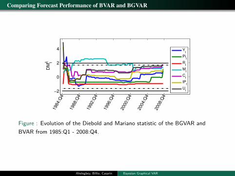
Comparing Forecast Performance of BVAR and BGVAR
−2
0
2
4 D
Mij t
1984:Q
4
1988:Q
4
1992:Q
4
1996:Q
4
2000:Q
4
2004:Q
4
2008:Q
4
Yt
Pit
Rt
Mt
Ct
IPt
Ut
Figure : Evolution of the Diebold and Mariano statistic of the BGVAR andBVAR from 1985:Q1 - 2008:Q4.
Ahelegbey, Billio, Casarin Bayesian Graphical VAR
Interconnectedness of the Financial System
Data : 19 super-sectors of Euro Stoxx 600 from January 2001 to August 2013,obtained from Datastream
Financial : Banks, Insurance, Financial Services and Real Estate
Non-Financial: Construction & Materials, Industrial Goods & Services,Automobiles & Parts, Food & Beverage, Personal & Household Goods,Retail, Media, Travel & Leisure, Chemicals, Basic Resources, Oil & Gas,Telecommunications, Health Care, Technology, Utilities
We estimate the model with lag length (p = 1) chosen according to the BICcriterion.
Compare MAR with pairwise (P-GC) and conditional Granger causality (C-GC)
Percentage of all possible links among the super-sectors
Linkages between Financial and Non-financial super-sectors
Following Billio et al. (2012), we use a 36-month moving window with an initialin-sample from January 2001 to December 2013
Ahelegbey, Billio, Casarin Bayesian Graphical VAR
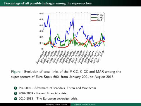
Percentage of all possible linkages among the super-sectors
0
0.1
0.2
0.3
0.4
0.5
0.6
Jan01−D
ec0
3
Jul0
1−Ju
n04
Jan02−D
ec0
4
Jul0
2−Ju
n05
Jan03−D
ec0
5
Jul0
3−Ju
n06
Jan04−D
ec0
6
Jul0
4−Ju
n07
Jan05−D
ec0
7
Jul0
5−Ju
n08
Jan06−D
ec0
8
Jul0
6−Ju
n09
Jan07−D
ec0
9
Jul0
7−Ju
n10
Jan08−D
ec1
0
Jul0
8−Ju
n11
Jan09−D
ec1
1
Jul0
9−Ju
n12
Jan10−D
ec1
2
Jul1
0−Ju
n13
P−GC
C−GC
MAR
Figure : Evolution of total links of the P-GC, C-GC and MAR among thesuper-sectors of Euro Stoxx 600, from January 2001 to August 2013.
1 Pre-2005 - Aftermath of scandals, Enron and Worldcom2 2007-2009 - Recent financial crisis3 2010-2013 - The European sovereign crisis.
Ahelegbey, Billio, Casarin Bayesian Graphical VAR
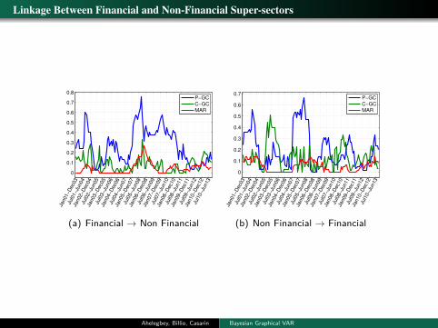
Linkage Between Financial and Non-Financial Super-sectors
0
0.1
0.2
0.3
0.4
0.5
0.6
0.7
0.8
Jan01−D
ec0
3
Jul0
1−Ju
n04
Jan02−D
ec0
4
Jul0
2−Ju
n05
Jan03−D
ec0
5
Jul0
3−Ju
n06
Jan04−D
ec0
6
Jul0
4−Ju
n07
Jan05−D
ec0
7
Jul0
5−Ju
n08
Jan06−D
ec0
8
Jul0
6−Ju
n09
Jan07−D
ec0
9
Jul0
7−Ju
n10
Jan08−D
ec1
0
Jul0
8−Ju
n11
Jan09−D
ec1
1
Jul0
9−Ju
n12
Jan10−D
ec1
2
Jul1
0−Ju
n13
P−GC
C−GC
MAR
(a) Financial → Non Financial
0
0.1
0.2
0.3
0.4
0.5
0.6
0.7
Jan01−D
ec0
3
Jul0
1−Ju
n04
Jan02−D
ec0
4
Jul0
2−Ju
n05
Jan03−D
ec0
5
Jul0
3−Ju
n06
Jan04−D
ec0
6
Jul0
4−Ju
n07
Jan05−D
ec0
7
Jul0
5−Ju
n08
Jan06−D
ec0
8
Jul0
6−Ju
n09
Jan07−D
ec0
9
Jul0
7−Ju
n10
Jan08−D
ec1
0
Jul0
8−Ju
n11
Jan09−D
ec1
1
Jul0
9−Ju
n12
Jan10−D
ec1
2
Jul1
0−Ju
n13
P−GC
C−GC
MAR
(b) Non Financial → Financial
Ahelegbey, Billio, Casarin Bayesian Graphical VAR

Comparing BIC Scores
−1400
−1300
−1200
−1100
−1000
−900
−800
Jan01−D
ec0
3
Jul0
1−Ju
n04
Jan02−D
ec0
4
Jul0
2−Ju
n05
Jan03−D
ec0
5
Jul0
3−Ju
n06
Jan04−D
ec0
6
Jul0
4−Ju
n07
Jan05−D
ec0
7
Jul0
5−Ju
n08
Jan06−D
ec0
8
Jul0
6−Ju
n09
Jan07−D
ec0
9
Jul0
7−Ju
n10
Jan08−D
ec1
0
Jul0
8−Ju
n11
Jan09−D
ec1
1
Jul0
9−Ju
n12
Jan10−D
ec1
2
Jul1
0−Ju
n13
P−GC
C−GC
MAR
Figure : BIC scores of P-GC, C-GC and MAR for linkages among thesuper-sectors of Euro Stoxx 600.
Ahelegbey, Billio, Casarin Bayesian Graphical VAR
Conclusion: Relevance of Results
Our graphical approach allows for inference of the lagged dependence andcontemporaneous structure from the data providing a natural way to insertrestriction in the VAR dynamics
The BGVAR is more parsimonious than the BVAR and the forecast performs aresignificantly equivalent.
Able to learn from the data the structure and sign restrictions on thecontemporaneous relationships
Not only are financial institutions highly interconnected before and during crisisperiods (Billio et al 2012)
Financial and Non-financial institutions are also highly interconnected duringsuch periods
Pairwise Granger causality (P-GC) overestimates links and Conditional Granger(C-GC) suffers due to over-fitting.
The MAR deliver satisfactory results on the causal structures by accounting forcausal uncertainties when applying Bayesian model averaging.
Ahelegbey, Billio, Casarin Bayesian Graphical VAR

Thank you !for your attention
Research supported by funding from the European Union, Seventh FrameworkProgramme FP7/2007-2013 under grant agreement SYRTO-SSH-2012-320270
Ahelegbey, Billio, Casarin Bayesian Graphical VAR

This project has received funding from the European Union’s Seventh Framework Programme for research, technological
development and demonstration under grant agreement n° 320270
www.syrtoproject.eu