Wage inequality, business strategy and productivity:
evidence from Portugal�
P. Ferreiray, J. Cerejeira, M. Portela, S. Sousa
Department of Economics, University of Minhoz
Preliminary version: please do not quote
3rd November 2014
Abstract
Using longitudinal linked employer-employee data we estimate �rm- and worker-e¤ects in wages using AKM methods of analysis. We then select di¤erent groupsof �rms, associated to di¤erent productivity levels and HRM pro�les, and identifydi¤erences across the groups both in terms the observed composition of the work-force and in terms of the estimated unobserved factors. Additionaly, we decomposewage inequality by the subgroups of �rms. Between group inequality explains avery small fraction of wage inequality. We follow up and analyse the contributionof the estimated e¤ects of observed and unobserved characteristics of workers and�rms to within group wage inequality. We conclude that time invariant unmeas-ured human capital is the major source of inequality within groups of �rms, yetdi¤erences in compensation policies across �rms (net of industry e¤ects) are also arelevant factor.
Keywords: Wage structure, human capital, productivity, HRM, LEED
JEL Classi�cation: C33, J31, J53
�Acknowledgments: This research was partially funded by Fundação para a Ciência e a Tecnolo-gia (Portugal) through the research project ref. no. PTDC/EGE-ECO/122126/2010 and the AppliedMicroeconomics Research Unit (NIMA), award no. PEst-OE/EGE/UI3181/2011.
yCorresponding author: Dept. of Economics, EEG �University of Minho, Braga 4710-057, Portugal.Email: [email protected], Phone: +351253601938, Fax: +351253601380
zFerreira is a¢ liated to the research unit NIMA; Cerejeira, Portela and Sousa are a¢ liated to theresearch unit NIPE.
1

1 Introduction
Signi�cant inter-industry wage di¤erentials are commonly found in most empirical ana-
lyses of wages using cross sectional data. The wage structure across industries can arise
as a consequence of imperfect measures of worker and �rm characteristics (Krueger and
Summers, 1988). That is, industries may di¤er on the type of workers employed or on the
compensation policies of �rms. These di¤erences may be responsible for the wage struc-
ture, e.g., high wage industries can either be hiring high wage workers or be composed
of high wage �rms, or have a combination of both. Previous research has attempted
to decompose wage di¤erentials paying particular attention to the structure (observed
characteristics) of �rms (Davis and Haltiwanger, 1991); others relate wages to di¤erent
supervision schemes across industries and �nds no evidence that interindustry di¤erences
in monitoring contribute to inter-industry wage di¤erentials which contradicts explan-
ations of industry wage premiums being caused by e¢ ciency wage models of shirking
(Neal, 1993). Groshen (1991) studies intraindustry establishment wage di¤erentials and
concludes that they are not random variations or returns to usual measures of human cap-
ital and suggests that further investigation is needed into inter-industry wage di¤erences
on sorting by unmeasured worker quality, compensating variations, e¢ ciency wages, and
rent-sharing.
Since the wage structure can be a consequence of omitted variable bias in cross-
sectional analyses, some authors attempt to identify the sources of the industry wage
structure using longitudinal linked employer-employee data. For example, Goux and
Maurin (1999) use French data and �nd that the wage structure is mainly due to un-
measured labour quality and that the potential wage gains from switching industries
would be less than 3%. Also using French data, Abowd et al. [AKM] (1999) conclude
that person e¤ects are relatively more important in explaining the di¤erentials found
in cross-sectional analyses. The same result is obtained by Abowd, Finer and Kramarz
(1999) with data for the State of Washington and applying the same decomposition as
AKM (1999). Controlling for worker-�rm match e¤ects Woodcock (2008)1 using Amer-
ican data �nds that �rm e¤ects are responsible for 72% of the variance in raw interindustry
wage di¤erentials, and Ferreira (2009) using Portuguese data �nds that 27% of the cross-
sectional wage di¤erences across industries are due to person unmeasured e¤ects and
70% of the wage structure are generated by �rm e¤ects.2 Overall, these studies provide
1In contrast with the other studies using linked employer-employee that disaggregate industry codingto a detailed level (more than 90 industries) Woodcock (2008) uses only 8 SIC Major Divisions.
2The di¤erence between the �ndings of Goux and Maurin (1999) and the other papers using matched
2
evidence that, after controlling for worker, �rm and match unobserved characteristics,
(true) inter-industry wage di¤erentials exist and persist over time. An industry can be
regarded as a wage contour and the industry wage e¤ect is determined by the pay policies
of �rms that compose the contour. However, empirical evidence suggests that �rms are
heterogeneous and that they di¤er with a high degree of persistence in several respects,
e.g., human resource management, productivity, and pay policies; while workers di¤er
in education, physical attributes and ability and human capital even within narrowly
de�ned industries (Doms et al., 1997; Syverson, 2011).
In this paper we use the Portuguese LEED Quadros de Pessoal to, �rstly, estimate
unobserved person- and �rm-e¤ects in wages using the AKM (1999) method. This allows
us to identify high- and low-wage �rms, and the industry wage structure. Secondly,
we analyse di¤erences and similarities of high-road and low-road industries and �rms
with respect to elements of human resources strategy. We investigate whether di¤erent
management structures, usually associated to higher-levels of productivity, are associated
to di¤erent pay policies of �rms (high- or low-wage �rms) within an industry. Following
Tor (2012), we identify di¤erent management strategies of �rms by focusing on contrasts
between: (i) exporters versus non-exporters; (ii) multi- vs single-plant �rms; (iii) foreign-
versus domestic-owned �rms.
Our results indicate the existence of a di¤erent wage structure across industries, after
controlling for time-invariant unobserved characteristics of the workers, which suggests
that the di¤erentials estimated from cross-sectional data are not due to compositional
e¤ects of the workforce and that di¤erent �rms pay di¤erent wages to workers with
the same characteristics (measured or unmeasured). This means that substantial wage
growth can be attained via mobility across industries. We also �nd considerable dis-
persion in �rm compensation policies within both high- and low-road industries. Given
this heterogeneity in �rm compensation policies within industries, and assuming that
di¤erences in productivity lead to di¤erences in wages, we followed up to describe and
decompose wage inequality into some of its components over mutually exclusive groups
of �rms de�ned according to productivity levels. Our results suggest there are di¤erences
across the groups of �rms both in terms the observed composition of the workforce and in
terms of the estimated unobserved factors. The results also indicate that between group
inequality explains a very small fraction of wage inequality, i.e., it is not the di¤erence in
worker-�rm data might be essentially due to the di¤erent techniques applied. The other studies usesimilar statistical methods to decompose the raw interindustry wage di¤erentials found in cross-sectionaldata.
3

productivity levels that generates the wage structure. The wage structure is mostly due
to some characteristics that are present in every group of �rms. When we analyse the
contribution of the estimated e¤ects of observed and unobserved characteristics of workers
and �rms to within group wage inequality we conclude that time invariant unmeasured
human capital is the major source of inequality within groups of �rms, yet di¤erences
in compensation policies across �rms (net of industry e¤ects) are also a relevant factor.
Therefore, it is by decreasing the di¤erences in the workforce human capital (transversal
skills, training, speci�c capital), that wage di¤erences would be reduced.
The paper is structured as follows. In the next section we describe the data used
and the statistical methods of the analysis. In section 3 we present and discuss our
results. Firstly we identify which �rms are high-wage and which are low wage and the
industry wage structure. Secondly, we describe di¤erences, both in terms of the observed
composition of the workforce and in terms of the estimated unobserved factors, across
subgroups of �rm pro�les. Thirdly, we describe wage inequality and decompose it (in
terms of between- and within-group inequality) by �rm type. We follow up and analyse
the contribution of the estimated unobserved �rm and worker e¤ects to within group
wage inequality. Section 4 summarizes and concludes our analysis.
2 Data and methods
2.1 Data
The main data set used in this analysis are the Quadros de Pessoal (QP) from Portugal,
a longitudinal data set with matched information on workers and �rms. These data have
been collected annually since 1985 by the Portuguese Ministry of Employment and the
participation of �rms with registered employees is compulsory. The data include all �rms
(over 250 thousand per year) and employees (more than two million per year) within
the Portuguese private sector. Each �rm and each worker have a unique registration
number which allows them to be traced over time. All information (on workers, plants,
and �rms) is reported by the �rm and, generally, relates to the situation observed in
the month when the survey is collected. The administrative nature of the data and
its public availability at the workplace, as determined by law, result in a high degree
of coverage and reliability. Information on workers includes, for example, gender, age,
educational level, quali�cations (skill), occupation, type of contract of employment, date
of entry to the �rm and date of last promotion, monthly hours of work and earnings
4
(split into a few components). Firm level data include, for example, the year of creation,
industry, location, total number of workers, number of establishments, sales volume, legal
structure and ownership structure (shares of participation of private, public or foreign
capital). We also use the International Trade data collected by the Portuguese O¢ ce
of National Statiscs (INE). This data set includes the universe of monthly export and
import transactions by �rms located in Portugal. Each transaction includes the �rm�s
identi�er making it possible combine this data with the QP data. For the purposes of
our analysis we use the data on export transactions to identify whether or not the �rm
is an exporter.
In our empirical analyses we estimate models with two-way �xed e¤ects. Abowd et al.
(2002) show that the identi�cation of the unobserved e¤ects using �xed e¤ects techniques
can be obtained by constructing groups of connected workers and �rms. Mobility of
workers across �rms is necessary for constructing such groups, each of which contains
all workers who have ever worked for any particular �rm and all the �rms at which any
particular worker was ever employed. We restrict our analysis to the biggest connected
group of workers and �rms for the years 2002 to 2009, and focus workers employed in
�rms operating within industries from the manufacturing and services sectors for which
there is non-missing information in the covariates relevant to our study. Our sample
contains 13,385,663 worker-year observations, relating to 3,323,016 workers and 246,564
�rms.3
Our dependent variable is the log hourly real wage (in euro) of the worker and is
constructed by adding up its components which are: (i) the base pay �gross amount
of money paid (in the reference month) to workers on a regular monthly basis for the
normal hours of work; (ii) tenure related payments; and (iii) regular payments. To obtain
the real hourly wages, the monthly wages are de�ated using the CPI and then divided by
the number of hours of work. The vector of observed time-varying covariates includes:
age and seniority at the �rm (and their squares), the type of contract of employment
(whether open- or closed-end contract), whether the worker works part- or full-time,
the skill level (low-, medium, high-skill), and the education level (ISCED1, ISCED2,
ISCED3, and ISCED5/6)4 We also control for �rm characteristics, such as: log of the
3Abowd et al. (2002) show that the identi�cation of the unobserved e¤ects using �xed e¤ects tech-niques can be obtained by constructing groups of connected workers and �rms. Mobility of workers across�rms is necessary for constructing such groups, each of which contains all workers who have ever workedfor any particular �rm and all the �rms at which any particular worker was ever employed. Since 93%of our original sample is part of the biggest connected group (the sample we work with), we concludethat there is considerable worker mobility in the economy.
4ISCED 1 � up to primary education, includes the �rst and second stages of basic education in
5

�rm size (size is measured by the number of workers employed by the �rm), the log of
real sales volume (in thousands of euro), ownership status (whether private, public or
foreign owned, depending on whether more than 50% of the �rms�social capital is owned
by private, public or foreign investors, respectively), whether the �rm is an exporter and
whether the �rm is multi-plant. Industry, region (NUTs I: North, Center, Lisbon and Tejo
Valley, Inland, Algarve, and Islands) and year dummies (2002-2009) are also included to
control for regional e¤ects and aggregate economic shocks. Descriptive statistics of our
sample are presented on Table 1.
[Table 1 about here]
Over the period the average hourly wage was 4.57 euro (hence its natural log is 1.52).
57% of the workers in our sample are males, the average age is 37 years and the mean
seniority at the �rm is nearly 8 years. Considering education and skill, 68% of the workers
have only up to 9 years os schooling (ISCED1 and 2), and about 11% of the workforce
has a university degree. The distribution of workers by skill levels is more even, 41%
of them are medium skilled and 21% high-skilled. As expected, a larger proportion
of workers are in open-ended contracts (73%) and in full-time jobs (97%). From these
statistics it seems that �rms in our sample prefer temporary-contracts (27%) to part-time
jobs (3%). Regarding the observed characteristics of �rms, the weighted mean of the real
sales volume of �rms in our sample is about 4 million euro (hence the natural log is 15,22)
and �rms employ, on average, 77 workers (ln �rm size is 4,34). About 47% of the workers
are on �rms that export, 38% in multi-establishment �rms and 12% of them in �rms
that are owned by foreigners. The majority of our workers are located in the Lisbon and
Tejo Valley (42%) and in the North Coast (28%) regions. Worker-year observations are
fairly evenly distributed across the years under analysis (proportions ranging between 11
and 14%). We use a �ne disaggregation of industry classi�cation and consider 46 distinct
industries. These are listed in Table 2 together with their relative frequencies in the data.
[Table 2 about here]
As we have mentioned before, we focus on two sectors of activity: manufacturing and
services. Looking at the distribution of the workers over these two sectors 71% of the
Portugal (up to 6 years of schooling); ISCED 2 �lower secondary education, includes the third stage ofbasic education (9 years of schooling); ISCED 3 �upper secondary education (12 years of schooling);ISCED 5/6 �higher education, includes �rst and second stages of tertiary education (more than 15 yearsof schooling corresponding to university degrees).
6

workers are employed in �rms providing services while the remaining 29% are employed
in manufacturing �rms. The industries that have larger shares of the workforce are
Construction (12,5%), Other business activities (10%), Retail (9%) and Wholesale (8%)
trade, and Hotels and restaurants (7%).
2.2 Empirical strategy
In the competitive model the wages of workers do not depend on �rm or industry a¢ li-
ation. This prediction is usually tested by de�ning a wage function as follows:
yijt = x�t� + k(j(i;t))�+ �ij (1)
where yijt is the logarithm of real hourly wages of worker i = 1; :::; N in �rm j = 1; :::; J
in period t = 1; :::; T ; x�t is the vector of observed time varying covariates of workers (i)
and �rms (j); k = 1; :::; K is a vector of mutually exclusive dummy variables indicating
the industry a¢ liation of �rm j; and �ij is the idiosyncratic error. If wages do not depend
on industry a¢ liation, then the parameters � should be jointly equal to zero. We test
this prediction in the next section.
If cross sectional industry e¤ects are statistically di¤erent from zero, raw-interindustry
wage di¤erentials exist. We proceed by investigating if these e¤ects hold after controlling
for unobserved e¤ects of workers and �rms. To this end we specify a competitive model
of wage determination that considers the longitudinal structure of the data and includes
observed characteristics of workers and �rms, as well as time invariant unobserved worker
and �rm characteristics as determinants of wages.5 The estimation of this model allows
for the identi�cation of �true� interindustry wage structure, that is, wage di¤erentials
that exist after controlling for the unobserved / unmeasured quality of the workers and
compensation policies of �rms. This structure is given by the average of the �rm e¤ects
within industries.
The person and �rm e¤ects model estimates a wage equation of the type:
y = X� +D� + F + � (2)
where y is a (N� � 1) vector of log monthly real wages (in deviations from the grand
mean); X(N��Z) is the matrix of observable time varying covariates (also in deviations
from the grand mean); D(N��N) is the matrix of indicators for worker i = 1; :::; N ; F(N��J)
5This section follows very closely the framework developed in AKM (1999).
7
is the matrix of indicators for the �rm at which worker i works at period t: The set of
parameters to estimate are �; the Z � 1 vector of coe¢ cients on the covariates; �, theN � 1 vector of worker e¤ects; , the J � 1 vector of �rm e¤ects. Worker e¤ects capture
time invariant characteristics of workers that a¤ect the worker�s wages in any �rm across
time, it is a portable component of compensation. Firm e¤ects capture time invariant
characteristics of �rms that a¤ect the wages of all workers within a �rm in the same way
across time. We can perform an orthogonal decomposition of the time invariant worker
e¤ects (�) into observable (�) and unobservable (�) components as follows:
�i = �i + �i�; (3)
where � can be interpreted as time invariant human capital or abilities of the worker that
are not measured in our survey, while � reports the e¤ects of observed time-invariant
covariates of the worker (which in our study are gender and education). A similar de-
composition can be made for the time invariant �rm e¤ects. Considering that each
industry is a wage contour, an industry e¤ect can be de�ned as a characteristic of the
�rm and the pure interindustry wage structure, conditional on the same information as
in equation (2), is de�ned as �k for some industry classi�cation k = 1; :::; K. Being a
characteristic of the �rm, it follows that the de�nition of the pure industry e¤ect (�k) is
the aggregation of the pure �rm e¤ects ( ) within the industry, that is
�k �NXi=1
TXt=1
�1(K(J(i; t)) = k) J(i;t)
Nk
�(4)
where
Nk �JXj=1
1(K(j) = k)Nj
and K(j) is a function denoting the industry a¢ liation of �rm j. This aggregation of J
�rm e¤ects into �k industry e¤ects, weighted so as to be representative of individuals, cor-
responds to including industry indicator variables in equation (2), �K(J(i;t)), and de�ning
what is left of the pure �rm e¤ect as a deviation from industry e¤ects, J(i;t) � �K(J(i;t))
(�rm e¤ects net of industry e¤ects).6
We will use our estimates of the pure interindustry wage structure to identify high- and
6Authors attempt to use industry classi�cations as detailed as to have more than 90 industry codes.The reason for decomposing industrial aggregates into the most detailed level possible is related to thepossibility that average compensation policies of �rms may vary across �ner levels of classi�cation andnot within aggregates, and so estimates can be subject to aggregation biases. The pure industry e¤ects,however, are not subject to this bias because they are computed from �rm-level estimates.
8
low-road industries. We will present alternative de�nitions of high/low-road industries
and describe them in terms of observed and unobserved characteristics. This allows the
identi�cation of similarities and di¤erences in behaviour and composition depending on
the business strategy. We then decompose the wage di¤erentials across high/low roads
in terms of within and between-inequality. Since our results suggest that most of the
wage di¤erences are due to within inequality (that is, wage structures regardless of the
business strategy type), we decompose the within-inequality in terms of shares due to
observed factors and unobserved characteristics of workers (human capital and ability)
and �rms (compensation policies).
3 Results
3.1 Firm compensation policies and the interindustry wage struc-
ture
To assess the existence of cross-sectional relative wages across industries we regress model
(1) on the annual data for the period from 2002 to 2009. The vector X includes covariates
on workers and �rms as described in subsection 2.1, and k assigns each �rm to each of
the K = 46 de�ned industries. An overview of the distribution of the year-on-year
raw interindustry wage di¤erentials is shown in Figure 1. Our estimates suggest the
existence of a cross sectional interindustry wage structure. The industry parameters are
jointly statistically signi�cant (yearly F-tests reject the hypothesis that the estimated
industry coe¢ cients are jointly equal to zero) and there is considerable dispersion on
the wage premia across industries. Considerable dispersion in raw-interindustry wage
di¤erentials was also found by Hartog et al. (2000) for the period 1982-1992 in Portugal,
the authors suggest these results are similar to those of countries with a decentralised
wage setting environment and note the potential �exibility to exploit industry (�rm)
speci�c conditions.
[Figure 1 about here]
However, as mentioned previously, wage di¤erentials obtained from cross-sectional
data may be generated by temporary disequilibrium in the labour market (thus being a
transitory phenomenon) or by systematic di¤erences in unobserved labour quality or in
�rm characteristics across industries (Krueger and Summers, 1998; Gibbons and Katz,
1992). Several studies have estimated wage equations where unobserved characteristics of
9
workers and �rms were controlled for and concluded that the composition of the workforce
was the main factor driving the inter-industry wage structure (Goux and Maurin, 1999;
AKM, 1999; Abowd, Finer and Kramarz, 1999). To investigate the existence of a �true�
interindustry wage structure, we have estimated a wage equation where we include time
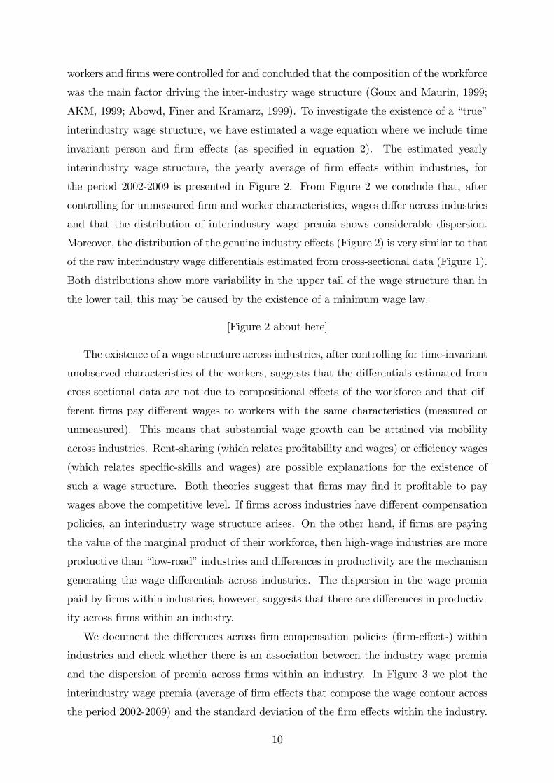
invariant person and �rm e¤ects (as speci�ed in equation 2). The estimated yearly
interindustry wage structure, the yearly average of �rm e¤ects within industries, for
the period 2002-2009 is presented in Figure 2. From Figure 2 we conclude that, after
controlling for unmeasured �rm and worker characteristics, wages di¤er across industries
and that the distribution of interindustry wage premia shows considerable dispersion.
Moreover, the distribution of the genuine industry e¤ects (Figure 2) is very similar to that
of the raw interindustry wage di¤erentials estimated from cross-sectional data (Figure 1).
Both distributions show more variability in the upper tail of the wage structure than in
the lower tail, this may be caused by the existence of a minimum wage law.
[Figure 2 about here]
The existence of a wage structure across industries, after controlling for time-invariant
unobserved characteristics of the workers, suggests that the di¤erentials estimated from
cross-sectional data are not due to compositional e¤ects of the workforce and that dif-
ferent �rms pay di¤erent wages to workers with the same characteristics (measured or
unmeasured). This means that substantial wage growth can be attained via mobility
across industries. Rent-sharing (which relates pro�tability and wages) or e¢ ciency wages
(which relates speci�c-skills and wages) are possible explanations for the existence of
such a wage structure. Both theories suggest that �rms may �nd it pro�table to pay
wages above the competitive level. If �rms across industries have di¤erent compensation
policies, an interindustry wage structure arises. On the other hand, if �rms are paying
the value of the marginal product of their workforce, then high-wage industries are more
productive than �low-road�industries and di¤erences in productivity are the mechanism
generating the wage di¤erentials across industries. The dispersion in the wage premia
paid by �rms within industries, however, suggests that there are di¤erences in productiv-
ity across �rms within an industry.
We document the di¤erences across �rm compensation policies (�rm-e¤ects) within
industries and check whether there is an association between the industry wage premia
and the dispersion of premia across �rms within an industry. In Figure 3 we plot the
interindustry wage premia (average of �rm e¤ects that compose the wage contour across
the period 2002-2009) and the standard deviation of the �rm e¤ects within the industry.
10

We �nd considerable dispersion in �rm compensation policies within both high- and
low-road industries suggesting that there is weak association between the industry wage
premia and the dispersion of compensation policies across �rms within an industry. In
fact, the correlation between the industry wage premia and the dispersion of �rm e¤ects
within industries is small and positive (0.14, as is re�ected by the small positive slope of
the linear prediction line depicted in Figure 3).
[Figure 3 about here]
Within the group of high-wage and low-dispersion industries (the median being the
threshold separating high/low-wage (high/low-dispersion)) we �nd: 41 Water collection,
treatment and distribution; 64 Post and telecommunications, 65 Financial intermediation
and 66 Insurance. These are industries with low levels of competition. Amongst the in-
dustries that pay, on average, high wages and have high dispersion in the premia paid,
the industries forming the wage contour include: 67Auxilliary activities to �nancial inter-
mediation; 61 Water transport; 63 Travel agents and tourism; 24 Chemicals and chemical
products. Within the set of low industry wage premia and low dispersion, we �nd low
value-added manufactures such as: 17 Textiles, 18 Manufacture of wearing apparel, dress-
ing and dying of fur; 19 Leather; and 36 Manufacture of furniture. Industries with low
wages and high dispersion in �rm compensation policies include: 45 Construction; 50
Sales and maintenance of vehicles; 52 Retail trade; 74 Other businesses; and 93 Other
services. This group involves a series of �rms that undertake various low value-added
businesses and services, and the mix of activities involved may be the cause of larger
dispersion in the compensation policies across �rms.
3.2 Measuring and decomposing wage di¤erentials: productiv-
ity of �rms and inequality
Firms are heterogeneous and empirical evidence suggests that they persistently di¤er in
several respects relating to, for example, their human resource management, productivity,
and pay policies (Syverson, 2011). The analysis in the previous section supports this
argument in that it concludes for the existence of di¤erent compensation policies across
�rms within industries. Assuming that di¤erences in productivity lead to di¤erences
in wages, in this section we describe and decompose wage inequality into some of its
components over mutually exclusive groups of �rms.7 Therefore, to inspect di¤erent
7Cowell and Fiorio (2010) provide a good survey on the decomposition approaches that we use.
11

behaviours of high- and low-road industries and �rms we �rst compare the top and bottom
5 industries, the top (bottom) include the 5 industries for which the estimated e¤ect (�)
is highest, while the bottom includes the 5 industries for which the estimated e¤ect is
lowest. We also compare the behaviour of the �rms that are ranked in the top (bottom)
decile of the distribution of the estimated �rm e¤ects ( ). However, the structure and
organisational form of the �rm is likely to a¤ect productivity (Garicano and Heaton
2007), as does the quality of the management practices and characteristics (Bloom and
Van Reenen 2007; Bertrand and Schoar 2003). The latter however are often unobserved in
surveys of �rms (Syverson 2011). To account for di¤erences in productivity we follow Tor
(2012) and focus on contrasts between: (i) exporting versus non-exporting �rms; ii) multi-
versus single-plant �rms; iii) foreign versus domestic owned �rms. Exporting �rms have
been shown to be more productive than non-exporting �rms even prior to exporting, and
the onset of exporting further raises productivity (Girma et al., 2004). Evidence suggests
that multi-establishment �rms are likely to have accumulated more knowledge about the
economic environment and may also have a more experienced management structure than
single establishment �rms (Audretsch and Mahmood, 1995), thus reducing their chances
of failure when faced with negative economic shocks. Previous research also suggests that
foreign-owned �rms have higher levels of productivity than home-owned, and �rms which
are acquired by foreign companies exhibit an increase in labour productivity of 13% (e.g.
Conyon, et al., 2002).
To measure wage inequality we adopt some alternative indicators: (i) the decile dis-
persion ratio (P90/P10); (ii) the Gini coe¢ cient; and (iii) generalized entropy measures:
Theil�s T and L. The decile dispersion ratio is computed as the ratio of the average real
hourly wage of the richest 10 percent group of workers to the average real hourly wage of
the poorest 10 percent of workers. Hence the decile dispersion ratio expresses the wages
of the top 10 percent (the �high-wage�) as a multiple of that of workers in the poorest
decile of the wage distribution (the �low-wage�). However, this ratio ignores information
about incomes in the middle of the wage distribution and does not use information about
the distribution of wages within the top and bottom deciles. The Gini coe¢ cient plots
the proportion of total wages that is cumulatively earned by the bottom x% of workers.
The lower the Gini coe¢ cient the more equal the distribution, with 0 corresponding to
complete equality, while higher Gini coe¢ cients indicate a more unequal distribution. For
example, a Gini coe¢ cient of 1 corresponds to one worker receiving 100% of total wages.
The Gini coe¢ cient may not be perfectly decomposable or additive across groups (when
12
ranking by subgroup wages overlaps a positive residual is generated, this has implications
for the decompositions of subsection 3.2.2). The Generalized Entropy (GE) measures
have the property of additive decomposability, that is, they are decomposable without a
residual term. The values of GE(�) measures vary between zero and in�nity, with zero
representing an equal distribution and higher values representing higher levels of inequal-
ity. The parameter � in the GE class represents the weight given to distances between
wages at di¤erent parts of the wage distribution and can take any real value. For lower
values of �, GE is more sensitive to changes in the lower tail of the distribution, and for
higher values of � GE is more sensitive to changes that a¤ect the upper tail. The most
common values of � used are 0, 1, and 2. GE(1) corresponds to Theil�s T index, GE(0)
is known as Theil�s L and is sometimes referred to as the mean log deviation measure.
In the sections that follow we �rst describe the various subgroups of the population in
terms of means of the observed and estimated factors, as well as in terms of correlations
between the unobserved e¤ects of workers and �rms (proxy for positive/negative sorting in
the labour market). We then compute various measures of inequality for the Portuguese
labour market overall and for the subgroups of the population we presented earlier in
this section. We follow up and decompose the overall structure of inequality in terms of
between and within group inequality and in terms of shares of contribution to inequality
by factors such as the observed covariates, the estimated time invariant (measured and
unmeasured) e¤ects of workers and �rms, and the unexplained part of the model.
3.2.1 Di¤erences in composition across partitions of the population
In this subsection we describe the di¤erent groups of the population in terms: (i) of the
time-varying observed characteristics of workers and �rms; (ii) of the e¤ects estimated
from the model speci�ed in equation (2); and (iii) of the pattern of sorting of workers
and �rms. The comparison of characteristics of workers and �rms helps establishing
di¤erences and similarities across types of business strategies and assess whether wages
and employment are a function of �rm productivity. The relevant statistics are presented
in Table 3.
[Table 3 about here]
Considering the set of observed covariates (�rst panel of Table 3), our results suggest
that more productive industries and �rms employ larger shares of highly-educated and
high-skilled workers, and have lower shares of workers in temporary contracts. Moreover,
13

they report higher sales volumes, and are on average larger �rms. The average wages
paid by the groups of more productive �rms pay are higher than those paid by the less
productive ones. Looking at the composition of the top (bottom) 5 industries (column
ii) the top 5 industries pay, on average, the double of the wage paid by the low-road
industries. The share of workers with university degrees in high-roads in 3 times larger
than that of the economy overall (34% vs 11%) and they use twice as much high-skilled
workers than that we observed for the economy-wide average (49% vs 21%). Within the
top 5 industries we �nd larger proportions of more productive �rms: exporters (54%), is
multiplant (86%), and foreign owned (21%) than what we observe in the economy overall.
On the other hand, low-roads employ only a very small share of highly-educated and high-
skilled workers (2% and 8%, respectively), and the proportion of more productive �rms
(multiplant, foreign owned) is also smaller. If instead we rank �rms in terms of their
compensation policies (column iii) we conclude that �rms in the top decile of the �rm-
e¤ects distribution have lower shares of temporary workers, larger shares of educated and
skilled workers, they are larger in size and have bigger sales volumes than �rms in the �rst
decile. The share of exporting, multiplant and foreign-owned �rms is also larger in the
top decile. When we describe our sample in terms of business strategy across industries,
i.e. whether �rms are exporting (column iv), multiplant (column v) or foreign owned
(column vi) the same sort of di¤erences arises. Therefore, both the high road industries
and the high-road �rms are composed, in terms of observed covariates, di¤erently from
their counterparts.
Inspection of the mean of the estimated e¤ects (second panel of Table 3) reveals that
the average of the e¤ects within high-road industries and �rms are above the economy-
wide average. High-roads perform better in terms of the observed time-varying charac-
teristics of workers and �rms (observed covariates), but they are also composed of better
workers and �rms with respect to the estimated time-invariant unmeasured e¤ects (the
unobserved human capital, �; and the �rm e¤ects net of industry e¤ects). For example,
the mean of the estimated unobserved human capital for the economy as a whole is 0.06,
whilst the mean in the top 5 industries is 0.35, in the top decile �rms is 0.08, for exporters
it is 0.09, for multiplant �rms is 0.10 and for foreign owned �rms is 0.11. Interestingly,
the estimated �rm e¤ects (net of industry e¤ects) are more or less similar across business
types.8 Overall, the lack of clear di¤erences in the component of the estimated �rm ef-
fects suggests that most di¤erences across business types may be generated by di¤erences
8These e¤ects are clearly di¤erent when we split the economy into the deciles of �rms, in column iii,this is explained by the splitting itself since it is done using the distribution of �rm e¤ects.
14

in characteristics of the workforce rather than in di¤erences in compensation policies of
�rms (this will be tested in subsection 3.2.3).
Considering the di¤erences in composition in the observed covariates and in the e¤ects
estimated from model speci�ed in equation (2) our results are in line with those of Doms
et al. (1997) in that workers in more productive �rms and industries have larger observed
and unobserved abilities. The existence of complementarities between workers abilities
and �rm productivity motivated our brief analysis on the type of matching, de�ned as
the correlation between the time invariant e¤ects of workers and �rms, observed across
the di¤erent groups of the population. There is positive assortative matching when the
most productive �rms employ the most skilled workers (Davidson et al., 2010). In our
setting, similar to Goux and Maurin (1999) and Abowd et al. (2002), this translates into
positive correlation coe¢ cients between worker and �rm estimated e¤ects. Considering
�rstly the economy overall (column i) we �nd a very small and positive (0.09) correlation
between the time-invariant worker and �rm e¤ects (� and ; respectively). But these
e¤ects include the time invariant characteristics of workers (gender and education) and
�rms (industry a¢ liation). The correlation of unmeasured human capital (�) and �rm
compensation policies ( ) is nearly zero, suggesting there is no assortative matching in
the labour market. Looking at the type of matching across high- and low-road industries
(column ii) there seems to be negative matching, that is, either we have high-wage workers
in low-wage industries (bottom 5 with correlations of -0.15 and -0.20) or we have low-
wage workers in high-wage industries (top 5 with correlations of -0.22 and -0.24), the same
type of conclusions can be reported when we split the sample into the top and bottom
decile of �rm e¤ects (column iii). Results are clearly di¤erent when our splitting of the
population is based on business strategies. We �nd positive assortative matching in �rms
that export (column iv), in the multi-establishment (column v) and in the foreign owned
�rms (column vi), and negative matching in their counterparts. Helpman et al. (2010)
argued that more productive �rms screen more intensely and have a workforce of higher
average ability than less productive �rms, which seems to be the case for these 3 types
of businesses. Our results suggest that these �rms seem to have larger returns to worker-
�rm complementarities, this must have increased their incentive to screen workers, hence
increase the matching quality.9
9Helpman (2010) and Davidson et al. (2010) also conclude that when the economy is opened totrade more productive �rms select into exporting, this increases their revenue relative to less productive�rms, which further increases the incentives to screen workers. Therefore exporting increases the wagespaid by a �rm with a given productivity. Overall, increased openness improves the e¢ ciency of matchingin the labour market (particularly whithin the group of more productive �rms with more comparative
15

3.2.2 Inequality within and between high- and low-roads
In this subsection we compute several measures of inequality and explore the structure
of inequality. We decompose the Theil�s T index (GE(1)) by subgroups of the popula-
tion (relating to di¤erent business strategies) to infer on the extent to which di¤erences
between the population sub-groups explain overall inequality in wages. In Table 4 we
describe the distribution of the population and of total wages across the subgroups we
de�ned previously, we also show the di¤erent measures of inequality (P90/P10 disper-
sion ratio, Gini, GE(0), G(1)) and decompose wage inequality (based on the Theil�s T
index (GE(1)) into within and between-group components. In such decomposition, the
component relating to between inequality captures the share of inequality that is due
to the variability of wages across the di¤erent sub-groups of the population, while the
component relating to within-inequality captures the share of overall inequality that is
due to the dispersion of wages within each sub-group of the population. The decompos-
ability requirements of inequality indices (Shorrocks, 1984) lead us to focus on one of the
Generalized Entropy indices, i.e., the Theil�s T index (GE(1)).10 Given the partitions of
the population the most general decomposition of an inequality index has the following
form
I = Iwithin + Ibetween + residual (5)
The GE indices are perfectly decomposable into within and between elements without
a residual term, and their decomposition can be expressed as
GE� =mXg=1
�ygy
�� �ngn
�1��GE(�)g +
1
�2 � �
mXg=1
�ygy
��ngn� 1!
(6)
where GE� is the overall GE index and GE(�)g is the GE index of the gth subgroup.
The �rst term on the RHS is the weighted average of the GE indices for each subgroup
g = 1; :::;m (where weights are represented by the total income share, i.e., the product of
population shares and relative mean incomes). This is the within part of the decomposi-
tion. The second term is the index calculated using the subgroup means instead of actual
wages, in order to capture variability amongst the groups, and it gives the between part
of the decomposition.
Our inequality indices and the decomposition of Theil�s T index are presented in Table
advantages).10Results on the decomposition on within and between components of inequality is similar using the
other GE index, G(0). Results can be shown upon request from the author.
16

4. The �rst column of the Table shows estimates of our inequality indices for the labour
market overall. The following three columns in the table report estimate of the Gini
coe¢ cient and the GE indices by sub-groups of the population according to exporting
status, whether or not the �rm is multi-plant and by ownership (whether national or
foreign capital). The labour market�s P90/P10 dispersion ratio reveals that workers in
the top decile of the wage distribution receive wages that are almost four times those
of workers in the bottom decile of the distribution. The estimate of the overall Gini
index for the labour market is 0,31 and the estimates of Theil�s L and T are 0,15 and 0,18
respectively. Looking at the inequality measures by groups of �rms (columns ii-iv), all our
indices suggest that there is more inequality in wages in the groups of �rms we associate
to higher productivity levels (exporters, multi-plant, and foreign-owned �rms) than in
the groups of �rms we associate to lower levels of productivity. Yet, the decomposition
of the Theil�s T index, GE(1), into within and between components indicates that over
94% of overall inequality comes from dispersion in wages within groups of �rms. That is,
wages are relatively equally distributed across types of business strategy and almost all
inequality comes from di¤erences in wages between workers within the groups of �rms.
[Table 4 about here]
Since inequality coming from wage di¤erences within groups of �rms has such a major
contribution to overall inequality, compared to inequality coming from di¤erences in wages
between groups of �rms, we will proceed with our analysis by decomposing the structure
of the within inequality into factor sources.
3.2.3 Factor source decomposition of within inequality: the role of unob-
served human capital and compensation policies
In this subsection we disaggregate within inequality into contributions of di¤erent factors.
This type of decomposition analysis of inequality is important for understanding the main
determinants of inequality. The determinants we consider are the set of components
estimated from model (2), the proportional decomposition of wage inequality is computed
as follows:
Cov(y; xb�)V ar(y)
+Cov(y;b�)V ar(y)
+Cov(y; b )V ar(y)
+Cov(y; �)
V ar(y)=V ar(y)
V ar(y)= 1; (7)
where cov (�) stands for covariance and var (�) stands for variance. The sum of the con-
tributions of the observed time varying covariates (xb�), the worker (b�) and �rm (b )17
time-invariant e¤ects, and the unexplained part of the model (�) give the aggregate in-
equality value, and their proportional contributions add up to one (Shorrocks, 1982).
Since we are interested in disentangling within inequality we perform this type of decom-
position by groups of �rms. The results are presented in Table 5. Columns (i) to (vi)
report the decompositions by type high- low-roads. As mentioned in Section 2.2 we can
decompose the time invariant e¤ects of workers and �rms into observable and unobserv-
able components (see, e.g., equation (3) for the worker e¤ects). Therefore, in Table 5
we perform such decompositions in order to identify the shares of inequality due to: (i)
observed characteristics of workers and �rms (including time-varying characteristics, and
the time invariant gender, education, and industry a¢ liation of the �rm) i.e., the share of
observed covariates combines the e¤ects of xb�+�b�+kb�; (ii) total worker invariant e¤ects(b�) and unmeasured human capital (b�); total �rm e¤ects (b ), and unmeasured compens-ation policies of the �rm (�rm e¤ects net of industry e¤ects:
�b � b��) this allows oneto infer on the importance of education and gender on the contribution of worker time
invariant e¤ects, and the importance of industry a¢ liation on the contribution of �rm
time invariant e¤ects.
[Table 5 about here]
Considering the economy overall (column i) wage di¤erentials can be decomposed
as follows: Unmeasured human capital (b�) accounts for the greatest share of the wagestructure we observed in the economy, 42% of the di¤erence in wages across workers is
due to this component. The second most important factor explaining the di¤erences in
wages across workers are the observed characteristics of workers and �rms, that account
for 38% of the di¤erentials. Within the observed component, education and gender
account for about 17p.p. (b�� b�) of the observed wage inequality and industry a¢ liationof the �rm (kb�) is responsible for about 7p.p. (20:42� 13:14) of the structure in wages.Compensation policies of the �rm that di¤er from the compensation policies common to
all �rms within each industry�b � b�� are responsible for 13% of the wage inequality.
Finally, 6% of the estimated inequality is not explained either observed or unobserved
components of the model. These results are in line with those obtained by Goux and
Maurin (1999), AKM (1999) and Abowd, Finer and Kramarz (1999) in that they suggest
that most of the di¤erences in wages are accounted for unmeasured human capital.
As mentioned in the previous section, we have an interest in investigating what is be-
hind the within inequality. That is, despite the partitions created according to di¤erent
productivity proxies, we concluded that most inequality was generated within groups of
18

the population rather than between groups. Hence, most of the observed wage di¤eren-
tials are not due to di¤erences in productivity across �rms but these exist within groups
of high- and low-road industries and �rms, they are transversal to the type of group-
ing we make. The decomposition of the di¤erentials within groups of the population is
presented in columns (ii) - (vi). Considering column ii, where we distinguish between the
industries that pay the highest and lowest wage premia in the economy, we realize that
within these two extremes observed characteristics of workers and �rms are responsible
for a smaller share of the wage di¤erences (when compared to the economy overall, col.
i), only 31% of the wage di¤erentials are explained by this component. The loss in ex-
planatory power of the observed characteristics is caused by the loss in importance of
industry a¢ liation (probably because it was the factor used for the division). We can see
that reduced explanatory power of industry a¢ liation if we compare the contribution of
the �rm e¤ect�b � and the net �rm e¤ect �b � b�� which are essentially the same around
11% for the bottom 5, and 7% for the top 5. Within these groups of the population the
largest share of the di¤erential is accounted for by the worker time invariant character-
istics (b� = 66%), and more than 50% is due to unmeasured human capital (b�). When wesplit the population into deciles of �rms, �rm unobserved e¤ects do not make a positive
contribution to wage inequality (as expected, since this grouping is based on the distribu-
tion of estimated �rm e¤ects). Within the two deciles (p90 or p10) the �rm compensation
policies contribute to equalizing the di¤erences in wages (contribution of �6%). On theother hand, time-invariant characteristics of the workers have their share increased and
more 76% of the di¤erentials in wages within these groups are accounted for worker time
invariant e¤ects, and at least 60% of that is accounted for unmeasured human capital.
Therefore when we have very homogeneous groups of �rms in terms of their compensation
policies (across industries), worker abilities become the major factor underlying the wage
structure. Our partitions of the population based on exporting, multiplant and foreign
ownership as proxies for productivity are also informative in that we realize that in the
more productive groups (exporters, multiplant and foreign owned) only about 5% of the
wage structure is not considered by our model. The contribution of worker time invariant
e¤ects, in general, and of unmeasured human capital, in particular, is largest in the most
productive groups than in their counterparts (and even larger than that observed in the
economy overall). Although using cross-sectional data, (Doms et al. 1997) �nd a similar
result in that they conclude that di¤erence in time invariant unobserved worker quality
are the main source of the cross-sectional correlation between productivity (technology
19

use) and worker wages. For exporters and multi-establishment �rms the contribution of
observed characteristics of workers and �rms is larger (38%) than that observed for the
non-exporters and single-plant �rms (35%). Firm compensation policies net of industry
e¤ects are also less powerful in determining wage di¤erentials within these groups (11%
for exporters and multiplant vs. 13% for the economy overall). In the case of foreign
owned �rms (column vi) there seems to be a trade-o¤ in the importance of observed char-
acteristics, which account for only 35% of the di¤erentials (compared to 38% in the other
partitions), and the �rm compensation policies (net of industry e¤ects) which account for
almost 15% of the wage structure - the largest contribution across all types of partitions
we have made.
Therefore, while in the previous section we have understood that most inequality
comes from within productivity groups of �rms, in this section we were able to demon-
strate that most of the inequality observed within groups of �rms (aggregated by pro-
ductivity levels) is induced by unobserved di¤erences in the workers�human capital. We
have also realized that whilst industry a¢ liation explains about 7% of the di¤erentials,
�rm-speci�c compensation policies are also important as they account for at least 11% of
the wage structure. Therefore, although changing �rms (or industry) may be a stepping
stone for wage growth, investments in human capital may have greater e¤ects for that
matter.
4 Conclusion
Using Portuguese LEED Quadros de Pessoal data under the AKM framework, we es-
timate unobserved person- and �rm-e¤ects identifying high- and low-wage �rms, and the
industry wage structure. Then, we analyse di¤erences and similarities of high-road and
low-road industries and �rms with respect to elements of human resources strategy. Our
results indicate the existence of di¤erent wage policies across industries, after controlling
for time-invariant unobserved characteristics of the workers, which suggests that the dif-
ferentials estimated from cross-sectional data are not due to compositional e¤ects of the
workforce and that di¤erent �rms pay di¤erent wages to workers with the same charac-
teristics (measured or unmeasured). This means that substantial wage growth can be
attained via mobility across industries. We also �nd considerable dispersion in �rm com-
pensation policies within both high- and low-road industries. Furthermore, the results
suggest di¤erences across the groups of �rms both in terms the observed composition of
20
the workforce and in terms of the estimated unobserved factors. We also conclude that
time invariant unmeasured human capital is the major source of inequality within groups
of �rms, yet di¤erences in compensation policies across �rms (net of industry e¤ects)
are also a relevant factor. Therefore, it is by decreasing the di¤erences in the workforce
human capital (transversal skills, training, speci�c capital), that wage di¤erences would
be reduced.
References
Abowd, John M., Robert H. Creecy and Francis Kramarz (2002) �Computing personand �rm e¤ects using linked longitudinal employer-employee data.� U.S. CensusBureau Technical Paper No. TP-2002-06.
Abowd, John M., Hampton Finer and Francis Kramarz (1999) �Individual and �rm het-erogeneity in compensation: an analysis of matched longitudinal employer-employeedata for the State of Washington.� in Haltiwanger, J. C., J. I. Lane, J. R. Splet-zer, J. J. M. Theeuwes and K. R. Troske (editors): The Creation and Analysis ofEmployer-Employee Matched Data. North-Holland, Amsterdam: 3-24.
Abowd, John M., Francis Kramarz and David N. Margolis (1999) �High wage workersand high wage Firms.�, Econometrica, 67(2): 251-333.
Audretsch, David B. and Talat Mahmood (1995) �New �rm survival: new results usinga hazard function.�, Review of Economics and Statistics, 77(1): 97-103.
Bertrand, Marianne and Antoinette Schoar (2003) �Managing with style: the e¤ect ofmanagers on �rm policies�, Quarterly Journal of Economics, 118(4): 1169-1208.
Bloom, Nicholas and John Van Reenen (2007) �Measuring and explaining managementpractices across �rms and countries�, Quarterly Journal of Economics 122(4): 1351-1408.
Conyon, Martin J., S. Girma, S. Thompson and P. W. Wright (2002) �The productiv-ity and wage e¤ects of foreign acquisition in the United Kingdom.�, Journal ofIndustrial Economics, 50(1): 85-102.
Cowell, Frank A. and C. V. Fiorio (2010) �Inequality decompositions: A Reconciliation�,Journal of Economic Inequality, 9(4): 509-528.
Davidson, Carl; Fredrik Heynman, Steven Matusz, Fredrik Sjöholm and Susan Zhu(2010) �Globalization and imperfect labor market sorting.�, Research Institute ofIndustrial Economics, IFN Working Paper No 856.
Davis, Steve J. and John Haltiwanger (1991) �Wage dispersion between and within U.S.manufacturing plants, 1963-1986�, in Martin Baily and Cli¤ord Winston (editors):Brookings papers on Economic Activity, Microeconomics:.115-200.
21

Doms, Mark; Timothy Dunne and Kenneth R. Troske (1997) �Workers, wages, andtechnology.�, Quarterly Journal of Economics, 112(1): 253-290.
Ferreira, Priscila (2009) �The sources of interindustry wage di¤erentials.�, ISER WPN.2009-13, Colchester, University of Essex.
Fiorio, Carlo V. and Stephen P. Jenkins (2010) �INEQRBD: Stata module to calcu-late regression-based inequality decomposition.�, Statistical Software ComponentsS456960, Boston College Department of Economics.
Garicano, Luis and Paul Heaton (2007) �Information technology, organization, and pro-ductivity in the public sector: evidence from police departments.�, Journal of LaborEconomics, 28(1): 167-201.
Girma, Sourafel; Avid Greenaway, and Richard Kneller (2004) �Does Exporting In-crease Productivity? A Microeconometric Analysis of Matched Firms.�, Review ofInternational Economics, 12(5): 855-866.
Gibbons, Robert and Lawrence Katz (1992) �Does unmeasured ability explain inter-industry wage di¤erentials?�, Review of Economic Studies, 59: 515-535.
Goux, Dominique and Eric Maurin (1999) �Persistence of interindustry wage di¤eren-tials: A reexamination using matched worker-�rm panel data.�, Journal of LaborEconomics, 17(3): 492-533.
Groshen, Erica L. (1991) �Sources of intra-industry wage dispersion: How much doemployers matter?�, Quarterly Journal of Economics, 106(3): 869-884.
Hartog, Joop; Pedro T. Pereira and José C. Vieira (2000) �Inter-industry wage dispersionin Portugal.�, Empirica, 27: 353-364.
Helpman, Elhanan; Oleg Itskhoki and Stephen Redding (2010) �Inequality and unem-ployment in a global economy�, Econometrica, 78(4): 1239-1283.
Jenkins, Stephen P. (2010) �INEQDEC0: Stata module to calculate inequality indiceswith decomposition by subgroup.�, Statistical Software Components S366007, Bo-ston College Department of Economics.
Krueger, Alan B. and Lawrence H. Summers (1988) �E¢ ciency wages and the inter-industry wage structure.�, Econometrica, 56(2): 259-293.
Shorrocks, A. F. (1984) �Inequality decomposition by population subgroups.�, Econo-metrica, 52(6): 1369-1385.
Syverson, Chad (2011) �What determines productivity?�, Journal of Economic Literat-ure, 49(2): 326-365.
Tor, Erikson (2012) �Progression of HR practices in Danish �rms during two decades�,unpublished paper, Aarhus University.
Woodcock, Simon (2008) �Wage di¤erentials in the presence of unobserved worker, �rmand match heterogeneity.�, Labour Economics, 15(4): 772-794.
22

Appendix: Tables and Figures
Table 1: Summary statisticsWorkers Mean Std Dev. Macroeconomic Mean Std Dev.
ln(real hourly wage) 1.52 0.51 Region
Age 37.74 11.10 North Coast 0.28
Tenure 7.66 8.37 Center Coast 0.15
Gender Lisbon & Tagus Valley 0.42
Male 0.57 Inland 0.07
Female 0.43 Algarve 0.04
Education Islands 0.04
ISCED1 0.46 Year
ISCED2 0.22 2002 0.11
ISCED3 0.21 2003 0.11
ISCED5/6 0.11 2004 0.12
Skill-level 2005 0.13
Low 0.37 2006 0.13
Medium 0.41 2007 0.13
High 0.21 2008 0.14
Type of contract of employment 2009 0.13
Open-end 0.73
Closed-end 0.27
Type of work
Full-time 0.97
Part-time 0.03
Firms
ln(real sales volume) 15.22 2.60
ln(�rm size) 4.34 2.15
Exporter
No 0.53
Yes 0.47
Multi-establishment
No 0.62
Yes 0.38
Ownership
National 0.88
Foreign 0.12
No. of worker-year obs 13,385,663
No. of workers 3,323,016
No. of �rms 246,564
23

Table 2: Summary statistics - industries at SIC2 levelIndustry description %
15 Manuf. of food, beverages and tobacco 3.69
17 Manuf. of textiles 2.91
18 Manuf. of wearing apparel; dressing and dying of fur 3.47
19 Tanning and dressing of leather; Manuf. of luggage, handbags, saddlery, harness and footwear 1.99
20 Manuf. of wood, products of wood & cork, except furniture; Manuf. of articles of straw & plaiting 1.43
21 Manuf. of pulp, paper and paper products 0.51
22 Publishing, printing and reproduction of recorded media 1.32
24 Manuf. of chemicals and chemical products, coke, re�ned petroleum products and nuclear fuel 0.97
25 Manuf. of rubber and plastic products 1.01
26 Manuf. of other non-metallic mineral products 2.12
27 Manuf. of basic metals 0.42
28 Manuf. of fabricated metal products, except machinery and equipment 2.96
29 Manuf. of machinery and equipment n.e.c 1.49
31 Manuf. of electrical machinery and apparatus n.e.c. 0.78
32 Manuf. of radio, television and communication equipment and apparatus 0.56
33 Manuf. of medical, precision and optical instruments, watches and clocks 0.22
34 Manuf. of motor vehicles, trailers and semi-trailers 1.32
35 Manuf. of other transport equipment 0.32
36 Manuf. of furniture; other manufacturing activities n.e.c. 1.72
37 Recycling 0.12
40 Production and distribution of electricity, gas, steam and hot water supply 0.25
41 Water collection, treatment and distribution 0.16
45 Construction 12.45
50 Sale. maintenance and repair of motor vehicles and motorcycles; retail sale of automotive fuel 3.60
51 Wholesale trade and commission trade, except of motor vehicles and motorcycles 7.56
52 Retail trade, except of motor vehicles and motorcycles; repair of personal and household goods 9.32
55 Hotels and restaurants 7.20
60 Land transport; transport via pipelines 3.12
61 Water transport 0.09
62 Air transport 0.47
63 Supporting and auxiliary transport activities; activities of travel agencies and other tourist activ. 1.46
64 Post and telecommunications 1.58
65 Financial intermediation, except insurance and pension funding 1.44
66 Insurance, pension funding and other complementary activities of social security 0.55
67 Activities auxiliary to �nancial intermediation 0.20
70 Real estate activities 0.67
71 Renting of machinery and equipment without operator, and of personal and household goods 0.31
72 Computer and related activities 0.98
73 Research and development 0.09
74 Other business activities 10.17
80 Education 1.74
85 Health and social work 4.64
90 Sewage and refuse disposal, sanitation and similar activities 0.21
91 Activities of membership organizations n.e.c. 0.72
92 Recreational. cultural and sporting activities 0.99
93 Other services 0.68
24

Table3:High-andlow-roads:descriptivestatistics
All
Industries
Firms
Firm:Exporter
Firm:Multi-plant
Firm:Ownership
(i)
(ii)
(iii)
(iv)
(v)
(vi)
Observedcovariates:
Bottom5
Top5
pct10
pct90
No
Yes
No
Yes
National
Foreign
ln(realhourlywage)
1.52
1.20
2.35
1.15
2.08
1.40
1.66
1.43
1.67
1.49
1.76
Woman
0.43
0.64
0.41
0.37
0.37
0.44
0.41
0.41
0.46
0.43
0.46
Age
37.74
37.58
39.01
38.06
38.86
37.6
37.92
37.85
37.58
37.97
36.05
Tenure
7.66
9.94
11.30
6.34
8.59
5.92
9.35
7.13
8.50
7.60
8.08
Close-end
0.27
0.18
0.10
0.24
0.22
0.31
0.23
0.28
0.27
0.28
0.26
ISCED
20.22
0.16
0.13
0.22
0.18
0.21
0.22
0.21
0.23
0.21
0.24
30.21
0.08
0.45
0.19
0.31
0.19
0.24
0.17
0.28
0.20
0.30
560.11
0.02
0.34
0.07
0.24
0.10
0.12
0.09
0.13
0.10
0.16
Skilllevel
medium
0.41
0.48
0.40
0.49
0.37
0.43
0.40
0.44
0.37
0.42
0.33
high
0.21
0.08
0.49
0.17
0.42
0.18
0.25
0.19
0.25
0.21
0.28
ln(realsalesvolume)
15.22
14.35
18.42
12.78
15.46
13.77
16.86
14.11
17.00
14.89
17.60
ln(size)
4.34
4.03
6.04
2.24
3.93
3.36
5.44
3.37
5.89
4.08
6.24
Exporter
0.47
0.64
0.54
0.17
0.47
��
0.36
0.64
0.42
0.86
Multi-plant
0.38
0.13
0.86
0.12
0.38
0.26
0.52
��
0.35
0.63
Foreignowner
0.12
0.08
0.21
0.02
0.18
0.03
0.22
0.07
0.20
��
Estimatede¤ects:
Observedcovariates
-0.03
-0.05
0.10
-0.12
-0.01
-0.09
0.03
-0.08
0.03
-0.05
0.06
Workere¤ects(�)
0-0.21
0.44
0.19
0.11
-0.05
0.05
-0.04
0.06
-0.01
0.09
observedtimeinvariant(�)
-0.06
-0.16
0.09
-0.07
0.03
-0.07
-0.04
-0.07
-0.04
-0.06
-0.02
unobs.humancapital(�)
0.06
-0.05
0.35
0.27
0.08
0.02
0.09
0.03
0.10
0.05
0.11
Firme¤ects( )
0.02
-0.08
0.28
-0.46
0.44
-0.00
0.04
0.01
0.03
0.01
0.07
Industry(�)
0.02
-0.08
0.28
-0.01
0.09
0.01
0.03
0.01
0.04
0.02
0.03
Firmnetofindustrye¤.
0-0.00
0.00
-0.45
0.35
-0.01
0.01
0.00
-0.01
-0.01
0.04
Correlationoftimeinvariante¤ects:
�vs.
0.09
-0.15
-0.22
-0.58
-0.24
-0.05
0.23
-0.03
0.28
0.04
0.36
�vs.
-0.01
-0.20
-0.24
-0.59
-0.28
-0.16
0.14
-0.14
0.19
-0.06
0.27
�vs.( ��)
-0.11
-0.20
-0.24
-0.60
-0.39
-0.23
0.02
-0.20
0.05
-0.16
0.17
No.ofobservations
13,385,663
1,442,767
338,963
366,645
1,063,719
7,111,232
6,274,431
8,256,113
5,129,550
11,770,622
1,615,041
Note:Sincemodelswereestimatedwithallvariables(dependentandindependent)indeviationsfrom
thegrandmeanE[Y]iszerointhemodelusingthefullsample,
Inpracticalterms,theexpectedvalueofwagesisgivenby
thesumoftheconstant(0.017)withtheestimated
e¤ectoftheobserved
covariates(-0.034)plusthe
estimated�rm
e¤ect(0.017).Di¤erencesinthemeansoftheestimatede¤ects,acrossgroupsofthepopulation,arestatisticallysigni�cantat1%
signi�cancelevel.
25

Table4:High-andlow-roads:measuresofinequalityinrealhourlywages
All
SIC2
SIC2
Firms
Firm:Exporter
Firm:Multi-plant
Firm:Ownership
(i)
(ii)
(iii)
(iv)
(v)
(vi)
(vii)
(46groups)
Bottom5
middle36
Top5
P10
interdecile
P90
No
Yes
No
Yes
National
Foreign
Workersshare(%)
1187
22.74
89.31
7.95
5347
6238
8812
Incomeshare(%)
787
61.74
84.39
13.87
4654
5545
8416
p90/p10
3.654
1.980
3.509
3.018
2.097
3.267
4.496
2.948
4.060
3.078
4.182
3.460
4.459
Gini
0.313
0.196
0.305
0.233
0.195
0.293
0.304
0.278
0.324
0.285
0.330
0.304
0.334
GE(0)Theil�sL
0.155
0.072
0.146
0.090
0.067
0.137
0.151
0.126
0.164
0.131
0.170
0.146
0.171
GE(1)Theil�sT
0.179
0.093
0.169
0.086
0.084
0.160
0.146
0.153
0.180
0.156
0.186
0.166
0.187
WithinandbetweendecompositionofTheil�sT
WithininequalityGE(1)
0.135
0.159
0.157
0.168
0.170
0.173
%oftotalinequality
75.4
89.1
87.7
93.9
95.0
96.7
BetweeninequalityGE(1)
0.044
0.019
0.022
0.011
0.009
0.005
%oftotalinequality
24.6
10.9
12.3
6.1
5.0
2.8
Note:ThedecompositionswerecomputedusingtheStatamoduleINEQDECObyJenkins(2010).
26
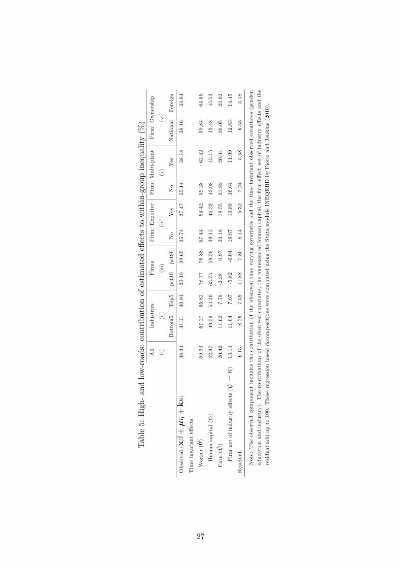
Table5:High-andlow-roads:contributionofestimatede¤ectstowithin-groupinequality(%)
All
Industries
Firms
Firm:Exporter
Firm:Multi-plant
Firm:Ownership
(i)
(ii)
(iii)
(iv)
(v)
(vi)
Bottom5
Top5
pct10
pct90
No
Yes
No
Yes
National
Foreign
Observed(x�+��+k�)
38.34
31.11
30.94
30.19
38.65
35.74
37.47
35.14
38.18
38.16
34.84
Timeinvariante¤ects
Worker(�)
59.90
67.27
65.82
78.77
76.38
57.44
64.42
59.23
62.42
59.84
64.55
Humancapital(�)
42.37
49.59
54.40
63.75
59.59
39.45
46.32
40.98
45.15
42.48
45.53
Firm( )
20.42
11.62
7.78
-2.38
0.97
23.18
18.55
21.82
20.04
20.05
22.02
Firmnetofindustrye¤ects( ��)
13.14
11.04
7.07
-5.82
-6.04
16.67
10.89
16.64
11.09
12.83
14.45
Residual
6.15
8.26
7.59
11.88
7.80
8.14
5.32
7.24
5.58
6.53
5.18
Note:Theobservedcomponentincludesthecontribution
oftheobservedtimevaryingcovariatesandthetimeinvariantobservedcovariates(gender,
education
andindustry).Thecontributionsoftheobservedcovariates,theunmeasuredhuman
capital,the�rm
e¤ectnetofindustrye¤ectsandthe
residualaddupto100.TheseregressionbaseddecompositionswerecomputedusingtheStatamoduleINEQRBDbyFiorioandJenkins(2010).
27

Figure 1: Raw interindustry wage di¤erentials, cross sectional speci�cation
21
01
23
Dis
tribu
tion
of ra
w in
dust
ry w
age
effe
cts
2002 2003 2004 2005 2006 2007 2008 2009Note. Standardized industry effects. Raw effects estimated from crosssectional specification. Excludes outside values.
Figure 2: �True�interindustry wage di¤erentials, AKM speci�cation
21
01
23
Dis
tribu
tion
of tr
ue in
dust
ry w
age
effe
cts
2002 2003 2004 2005 2006 2007 2008 2009Note. Standardized industry effects. True effects estimated from the person & firm effects model. Excludes outside values.
28

Figure 3: Association between the dispersion of �rm e¤ects and the industry wage premia
36
18
93
1917
55
5274
4550
2885
35
15
34
33
2071
29
70
32
60
27
51
26
91
31
22
62
25
21
72
37
80
7390
92
64
6324
41
61
67
66
65
40
0.09
0.28
med
ian=
.18
Stan
dard
dev
iatio
n of
firm
effe
cts
with
in in
dust
ies
1.68 2.26median=.16Standardized industry effects (mean of firm effects)
Dispersion Fitted values
29
Recommended