Volatility Modeling Using the Student’s t Distribution
Maria S. Heracleous
Dissertation submitted to the Faculty of the
Virginia Polytechnic Institute and State University
in partial fulfillment of the requirements for the degree of
Doctor of Philosophy
in
Economics
Aris Spanos, Chair
Richard Ashley
Raman Kumar
Anya McGuirk
Dennis Yang
August 29, 2003
Blacksburg, Virginia
Keywords: Student’s t Distribution, Multivariate GARCH, VAR, Exchange Rates
Copyright 2003, Maria S. Heracleous

Volatility Modeling Using the Student’s t Distribution
Maria S. Heracleous
(ABSTRACT)
Over the last twenty years or so the Dynamic Volatility literature has produced a wealth of uni-variate and multivariate GARCH type models. While the univariate models have been relativelysuccessful in empirical studies, they suffer from a number of weaknesses, such as unverifiable param-eter restrictions, existence of moment conditions and the retention of Normality. These problemsare naturally more acute in the multivariate GARCH type models, which in addition have theproblem of overparameterization.
This dissertation uses the Student’s t distribution and follows the Probabilistic Reduction (PR)methodology to modify and extend the univariate and multivariate volatility models viewed asalternative to the GARCH models. Its most important advantage is that it gives rise to internallyconsistent statistical models that do not require ad hoc parameter restrictions unlike the GARCHformulations.
Chapters 1 and 2 provide an overview of my dissertation and recent developments in the volatil-ity literature. In Chapter 3 we provide an empirical illustration of the PR approach for modelingunivariate volatility. Estimation results suggest that the Student’s t AR model is a parsimoniousand statistically adequate representation of exchange rate returns and Dow Jones returns data.Econometric modeling based on the Student’s t distribution introduces an additional variable −the degree of freedom parameter. In Chapter 4 we focus on two questions relating to the ‘degree offreedom’ parameter. A simulation study is used to examine: (i) the ability of the kurtosis coefficientto accurately capture the implied degrees of freedom, and (ii) the ability of Student’s t GARCHmodel to estimate the true degree of freedom parameter accurately. Simulation results reveal thatthe kurtosis coefficient and the Student’s t GARCH model (Bollerslev, 1987) provide biased andinconsistent estimators of the degree of freedom parameter.
Chapter 5 develops the Students’ t Dynamic Linear Regression (DLR) model which allows usto explain univariate volatility in terms of: (i) volatility in the past history of the series itself and(ii) volatility in other relevant exogenous variables. Empirical results of this chapter suggest thatthe Student’s t DLR model provides a promising way to model volatility. The main advantage ofthis model is that it is defined in terms of observable random variables and their lags, and notthe errors as is the case with the GARCH models. This makes the inclusion of relevant exogenousvariables a natural part of the model set up.
In Chapter 6 we propose the Student’s t VAR model which deals effectively with several keyissues raised in the multivariate volatility literature. In particular, it ensures positive definiteness ofthe variance-covariance matrix without requiring any unrealistic coefficient restrictions and providesa parsimonious description of the conditional variance-covariance matrix by jointly modeling theconditional mean and variance functions.
Acknowledgments
I am extremely grateful to my advisor, Aris Spanos, for encouraging me to pursue a Ph.D. and
helping me navigate through the complex field of Econometrics. His inspiring teaching and invalu-
able advice have been absolutely vital for the development of this research. My special thanks also
go to Anya McGuirk for her genuine commitment, constructive suggestions and her enthusiastic
support that enabled me to complete my dissertation.
I would like to thank my other committee members, Richard Ashley, Raman Kumar and Dennis
Yang for their valuable suggestions and interest in my work. I am also grateful to Abon Mozumdar
and Andrew Feltenstein who were originally on my committee and gave me guidance when I first
started working on this dissertation.
My sincere thanks go to Sudipta Sarangi for his entertaining phone calls and constant encour-
agement, and to Andreas Koutris for making sure I had fun while writing the dissertation. I am
also thankful to the staff members of our department: Sherry Williams, Barbara Barker and Mike
Cutlip for all their assistance. The department would not be the same without them.
Special thanks go to my roommates: Ana Martin, for her endless stories during my first year
of adjustment in Blacksburg and Yea Sun Chung for her patience during my last year of writing.
For the three years in between I am particularly thankful to Stavros Tsiakkouris who helped me
with all kinds of little things and made my life in Blacksburg hi-tech, easier and fun!
Last but not least, I would like to thank my parents, Stelios and Panayiota, who have taught
me the important things in life and have supported all my endeavors. My parents and my sister
Elpida have given me great affection and support while patiently enduring my long absence from
home.
iii

Contents
1 Introduction 1
1.1 Background . . . . . . . . . . . . . . . . . . . . . . . . . . . . . . . . . . . . . . . . . 1
1.2 Econometrics of Multivariate Volatility Models . . . . . . . . . . . . . . . . . . . . . 5
1.3 A Brief Overview . . . . . . . . . . . . . . . . . . . . . . . . . . . . . . . . . . . . . . 8
2 Towards a Unifying Methodology for Volatility Modeling 14
2.1 Introduction . . . . . . . . . . . . . . . . . . . . . . . . . . . . . . . . . . . . . . . . . 14
2.2 GARCH Type Models: Univariate . . . . . . . . . . . . . . . . . . . . . . . . . . . . 16
2.3 GARCH Type Models: Multivariate . . . . . . . . . . . . . . . . . . . . . . . . . . . 21
2.4 Probabilistic Reduction Approach . . . . . . . . . . . . . . . . . . . . . . . . . . . . 32
2.4.1 The VAR(1) from the Probabilistic Reduction Perspective . . . . . . . . . . . 36
2.5 Conclusion . . . . . . . . . . . . . . . . . . . . . . . . . . . . . . . . . . . . . . . . . 38
3 Univariate Volatility Models 40
3.1 Introduction . . . . . . . . . . . . . . . . . . . . . . . . . . . . . . . . . . . . . . . . . 40
3.2 A Picture’s Worth a Thousand Words . . . . . . . . . . . . . . . . . . . . . . . . . . 41
3.3 Statistical Model Comparisons . . . . . . . . . . . . . . . . . . . . . . . . . . . . . . 53
3.3.1 Normal Autoregressive Model . . . . . . . . . . . . . . . . . . . . . . . . . . . 54
3.3.2 Heteroskedastic Models . . . . . . . . . . . . . . . . . . . . . . . . . . . . . . 55
iv

3.3.3 Student’s t Autoregressive Model with Dynamic Heteroskedasticity . . . . . . 57
3.4 Empirical Results . . . . . . . . . . . . . . . . . . . . . . . . . . . . . . . . . . . . . . 59
3.5 Conclusion . . . . . . . . . . . . . . . . . . . . . . . . . . . . . . . . . . . . . . . . . 69
4 Degrees of Freedom, Sample Kurtosis and the Student’s t GARCH Model 70
4.1 Simulation Set Up . . . . . . . . . . . . . . . . . . . . . . . . . . . . . . . . . . . . . 71
4.1.1 Theoretical Questions . . . . . . . . . . . . . . . . . . . . . . . . . . . . . . . 71
4.1.2 Data Generation . . . . . . . . . . . . . . . . . . . . . . . . . . . . . . . . . . 72
4.2 Results . . . . . . . . . . . . . . . . . . . . . . . . . . . . . . . . . . . . . . . . . . . . 74
4.2.1 Estimates of α4 and the Implied Degrees of Freedom . . . . . . . . . . . . . . 75
4.2.2 Estimates of the Student’s t GARCH parameters . . . . . . . . . . . . . . . . 76
4.3 Conclusion . . . . . . . . . . . . . . . . . . . . . . . . . . . . . . . . . . . . . . . . . 82
5 Student’s t Dynamic Linear Regression 83
5.1 Student’s t DLR Model . . . . . . . . . . . . . . . . . . . . . . . . . . . . . . . . . . 84
5.1.1 Specification . . . . . . . . . . . . . . . . . . . . . . . . . . . . . . . . . . . . 84
5.1.2 Maximum Likelihood Estimation . . . . . . . . . . . . . . . . . . . . . . . . . 88
5.2 Empirical Results . . . . . . . . . . . . . . . . . . . . . . . . . . . . . . . . . . . . . . 91
5.2.1 Data and Motivation . . . . . . . . . . . . . . . . . . . . . . . . . . . . . . . . 91
5.2.2 Empirical Specification and Results . . . . . . . . . . . . . . . . . . . . . . . 92
5.3 Conclusion . . . . . . . . . . . . . . . . . . . . . . . . . . . . . . . . . . . . . . . . . 106
6 The Student’s t VAR Model 107
6.1 Introduction . . . . . . . . . . . . . . . . . . . . . . . . . . . . . . . . . . . . . . . . . 107
6.2 Statistical Preliminaries . . . . . . . . . . . . . . . . . . . . . . . . . . . . . . . . . . 108
6.2.1 Matrix Variate t distribution . . . . . . . . . . . . . . . . . . . . . . . . . . . 109
6.2.2 Some Important Results on Toeplitz Matrices . . . . . . . . . . . . . . . . . . 115
v

6.2.3 Matrix Calculus and Differentials . . . . . . . . . . . . . . . . . . . . . . . . . 118
6.3 Student’s t VAR Model . . . . . . . . . . . . . . . . . . . . . . . . . . . . . . . . . . 121
6.3.1 Specification . . . . . . . . . . . . . . . . . . . . . . . . . . . . . . . . . . . . 121
6.3.2 Maximum Likelihood Estimation . . . . . . . . . . . . . . . . . . . . . . . . . 130
6.4 Statistical Model Comparisons . . . . . . . . . . . . . . . . . . . . . . . . . . . . . . 134
6.5 Conclusion . . . . . . . . . . . . . . . . . . . . . . . . . . . . . . . . . . . . . . . . . 137
7 Conclusion 139
A Student’s t VAR Derivatives 156
vi

List of Figures
3-1 Standardized t-plot (DEM) . . . . . . . . . . . . . . . . . . . . . . . . . . . . . . . . . . 43
3-2 Standardized t-plot (FRF) . . . . . . . . . . . . . . . . . . . . . . . . . . . . . . . . . . 43
3-3 Standardized t-plot (CHF) . . . . . . . . . . . . . . . . . . . . . . . . . . . . . . . . . . 44
3-4 Standardized t-plot (GBP) . . . . . . . . . . . . . . . . . . . . . . . . . . . . . . . . . . 44
3-5 Standardized Normal P-P plot (FRF) . . . . . . . . . . . . . . . . . . . . . . . . . . . . 46
3-6 Standardized Student’s t P-P plot, ν = 6, (FRF) . . . . . . . . . . . . . . . . . . . . . . 46
3-7 Standardized Student’s t P-P plot, ν = 7, (FRF) . . . . . . . . . . . . . . . . . . . . . . 47
3-8 Standardized Student’s t P-P plot, ν = 8, (FRF) . . . . . . . . . . . . . . . . . . . . . . 47
3-9 Standardized t-plot (DJ) . . . . . . . . . . . . . . . . . . . . . . . . . . . . . . . . . . . 49
3-10 Standardized Normal P-P plot (DJ) . . . . . . . . . . . . . . . . . . . . . . . . . . . . . 49
3-11 Standardized Student’s t P-P plot, ν = 3, (DJ) . . . . . . . . . . . . . . . . . . . . . . . 50
3-12 Standardized Student’s t P-P plot, ν = 4, (DJ) . . . . . . . . . . . . . . . . . . . . . . . 50
3-13 Standardized Student’s t P-P plot, ν = 5, (DJ) . . . . . . . . . . . . . . . . . . . . . . . 51
4-1 Kernel density for nu, ν = 6, σ2 = 1, n = 50 . . . . . . . . . . . . . . . . . . . . . . . . 79
4-2 Kernel density for nu, ν = 6, σ2 = 1, n = 100 . . . . . . . . . . . . . . . . . . . . . . . 79
4-3 Kernel density for nu, ν = 6, σ2 = 1, n = 500 . . . . . . . . . . . . . . . . . . . . . . . 80
4-4 Kernel density for nu, ν = 6, σ2 = 1, n = 1000 . . . . . . . . . . . . . . . . . . . . . . . 80
4-5 Kernel density for nu, ν = 6, σ2 = 0.25, n = 500 . . . . . . . . . . . . . . . . . . . . . 81
vii

4-6 Kernel density for nu, ν = 6, σ2 = 4, n = 500 . . . . . . . . . . . . . . . . . . . . . . . 81
viii

List of Tables
2.1 The PR Approach: Normal VAR(1) Model . . . . . . . . . . . . . . . . . . . . . . . 38
3.1 Degrees of Freedom: P-P Plots and Sample Kurtosis Coefficient . . . . . . . . . . . . 52
3.2 Descriptive Statistics: Exchange Rates and Dow Jones . . . . . . . . . . . . . . . . . 52
3.3 Correlation Matrix: Exchange Rates . . . . . . . . . . . . . . . . . . . . . . . . . . . 53
3.4 Reduction and Probability Model Assumptions: Normal AR . . . . . . . . . . . . . . 54
3.5 Reduction and Probability Model Assumptions: Student’s t AR . . . . . . . . . . . 58
3.6 OLS Estimations: AR(2) and AR(3) . . . . . . . . . . . . . . . . . . . . . . . . . . . 60
3.7 Misspecification Tests for AR Models . . . . . . . . . . . . . . . . . . . . . . . . . . . 61
3.8 Estimation Results: Normal ARCH(5) . . . . . . . . . . . . . . . . . . . . . . . . . . 62
3.9 Misspecification Testing: ARCH(5) . . . . . . . . . . . . . . . . . . . . . . . . . . . . 63
3.10 Estimation Results and Misspecification Tests: Normal GARCH(1,1) . . . . . . . . . 64
3.11 Estimation Results and Misspecification Tests: Student’s t GARCH . . . . . . . . . 66
3.12 Estimation Results and Misspecification Tests: Student’s t AR Models . . . . . . . . 68
4.1 Descriptive Statistics for Sample Kurtosis and inu . . . . . . . . . . . . . . . . . . . 75
4.2 Descriptive Statistics for Estimated nu . . . . . . . . . . . . . . . . . . . . . . . . . . 77
4.3 Descriptive Statistics for the Student’s t GARCH parametes, n=500 . . . . . . . . . 78
4.4 Descriptive Statistics for the constant in the Student’s t GARCH model, n=500 . . . 78
5.1 The PR Approach: Student’s t DLR Specification . . . . . . . . . . . . . . . . . . . . 87
ix

5.2 Reduction and Probability Model Assumptions: Student’s t DLR . . . . . . . . . . . 88
5.3 Normal DLR: Exchange Rates 1973-1991 . . . . . . . . . . . . . . . . . . . . . . . . . 93
5.4 Normal DLR: Exchange Rates 1986-2000 . . . . . . . . . . . . . . . . . . . . . . . . . 94
5.5 Student’s t DLR: Exchange Rates 1973-1991 . . . . . . . . . . . . . . . . . . . . . . 96
5.6 Student’s t DLR: Deutschemark and French Franc 1986-2000 . . . . . . . . . . . . . 97
5.7 Student’s t DLR: Deutschemark and Swiss Franc 1986-2000 . . . . . . . . . . . . . . 98
5.8 Student’s t DLR: French Franc and Swiss Franc 1986-2000 . . . . . . . . . . . . . . 99
5.9 Student’s t AR: Exchange Rates 1973-1991 . . . . . . . . . . . . . . . . . . . . . . . 101
5.10 Student’s t AR: Exchange Rates 1986-2000 . . . . . . . . . . . . . . . . . . . . . . . 101
5.11 Normal GARCH-X: Exchange Rates 1973-1991 . . . . . . . . . . . . . . . . . . . . . 103
5.12 Normal GARCH-X: Exchange Rates: 1986-2000 . . . . . . . . . . . . . . . . . . . . . 103
5.13 Normal DLR and Student DLR: Dow Jones and T-bill rate . . . . . . . . . . . . . . 105
5.14 Normal GARCH(1,1)-X: Dow Jones and T-bill rate . . . . . . . . . . . . . . . . . . . 105
6.1 The PR Approach: Student’s t VAR(1) Specification . . . . . . . . . . . . . . . . . . 129
6.2 Reduction and Probability Model Assumptions: Student’s t VAR . . . . . . . . . . 130
x

Chapter 1
Introduction
1.1 Background
Modeling, analyzing, and forecasting volatility has been the subject of extensive research among
academics and practitioners over the last twenty years. Typically volatility models provide volatility
forecasts. This information is used in risk management, derivative pricing and hedging, portfolio
selection and even policy making. But what precisely do we mean by volatility in Economics and
Finance? After all, as Granger (2002, p.452) pointed out “volatility is not directly observed or
publicly recorded.” The term has been used by numerous researchers in different contexts and it is
not clear that they all refer to the same attribute. To understand volatility we need to consider
how one can measure volatility from observed data by linking it to concepts of uncertainty and
risk. Volatility1, as being used in everyday language, refers to variability in prices or returns such
as stock returns and exchange rate returns. The most popular measure of this type of volatility
is the standard deviation. Other commonly used measures include the interquartile range and the
mean absolute return.
In order to model volatility rigorously we need to consider its two different dimensions: (i)
univariate volatility, which involves only a single series, and (ii) multivariate volatility, which
1Volatility is often equated to uncertainty although this connection is debatable. The link between volatility andrisk is even more tenuous, in particular, volatility exists both in the upper and lower tail of the returns distributionbut risk is often associated only with the lower tail of the distribution.
1

involves the interactions of multiple series. For example, one may consider a case where volatility
in the United States stock market may be only affected by volatility observed in the United States
stock market on the previous day. This is univariate volatility − it involves only the past history ofthe series itself! A more realistic scenario today however, would be to consider the situation where
volatility in the United States stock market is affected by its own history as well as volatilities
observed earlier in the Asian and European markets. This is an example of multivariate volatility
since it involves not only the past history of volatilities but correlations among other variables as
well. Engle, Ito and Lin (1990b) refer to these as “heat waves” and “meteor shower effects”. The
Asian financial crisis, of 1996-1997, is an excellent example of a “meteor shower effect” since it
involves financial volatility transmission between foreign exchange markets. Fleming and Lopez
(1999) find that unlike London and Tokyo, yield volatilities for US treasury bills in New York do
not depend on global factors and hence can be characterized by “heat waves”.
Another example of multivariate volatility arises naturally when we consider several assets in
the same market. One can argue that each individual stock is influenced by the volatility of the
market as a whole as well as its own volatility − temporal variations in idiosyncratic volatility.
This is a natural implication of the Capital Asset Pricing Model (CAPM). To clearly understand
this kind of phenomena we really need to consider the notion of multivariate volatility.
In the last two decades there has been an explosion in volatility research. The “Dynamic
Volatility Era”2 began with the introduction of the Autoregressive Conditional Heteroskedastic
Model (ARCH), by Engle in 1982. The ARCH(p) model expresses the conditional variance as a
p−th order weighted average of past (squared) disturbances and thus is able to describe volatilityclustering3 in financial series. Following this, an enormous body of research has focused on extend-
ing and generalizing the ARCH model, mainly by providing alternative functional forms for the
conditional variance. Some of the most important contributors to the dynamic volatility literature
have been Engle, Bollerslev, Nelson and Ding. Bollerslev (1986) proposed the Generalized ARCH
(GARCH), as a more parsimonious way of modeling volatility dynamics. A limitation of both
2Andreou, Pittis and Spanos (2001) identify three distinct periods since the early twentieth century in relation tothe modeling of speculative prices. The next chapter provides a brief description of these different historical eras involatility modeling.
3Volatility clustering refers to the tendency for large (small) price changes to be followed by other large (small)price changes (see Mandelbrot, (1963)).
2

the ARCH and the GARCH models is that they only use information on the magnitude of the
returns while completely ignoring information on the sign of the returns. To remedy this Nelson
(1991) introduced the Exponential GARCH (EGARCH) model, which was the first in the family
of asymmetric4 GARCH models.
During this period a number of advancements were also made in other areas of the volatility
literature. One important contribution was the development of theoretical results regarding the sta-
tistical properties of the most popular ARCH and Stochastic Volatility models (Drost and Nijman
1993, Nelson 1990), as well as the development of MLE, QMLE, Bayesian, and Adaptive Estimation
procedures (see for example Geweke (1989) and Bollerslev and Wooldridge (1992)). Another major
development has been the extension to the family of multivariate GARCH models. The advantage
of the multivariate framework is that it can model temporal dependencies in the conditional co-
variances as well as the conditional variances. Although the multivariate models provide a better
description of reality, they unfortunately suffer from the overparametrization problem.
The most significant contribution of this extensive volatility research is that now we have a much
clearer and better understanding of the probabilistic features of speculative returns data. This is of
crucial importance in the search for an overarching framework, which will be able to first capture the
empirical regularities adequately, and ultimately give us reliable volatility forecasts. The extensions
and modifications of the GARCH family of models are numerous, and some discussion of the most
popular ones can be found in Chapter 2. There are also a number of extensive surveys5 of the
literature including for instance Bollerslev, Chou and Kroner (1992a), Bollerslev Engle and Nelson
(1994a), and Ding and Engle (2001).
The flurry of research in modeling dynamic volatility and the impact of the GARCH family
of models should not be surprising. Volatility is topical, and naturally relevant to modeling and
forecasting economic and financial phenomena. It plays a major role in investment security valua-
tion, risk management and the formation of monetary policy. For example in the US, the Federal
Reserve takes into account the volatility of stocks, bonds, currencies and commodities in establish-
ing monetary policy (Nasar, 1992). Similarly the Bank of England has made frequent references to
4Other asymmetric models include the Threshold ARCH (TARCH), by Rabemananjara and Zakoian (1993), andGlosten, Jaganathan and Runkle (1993).
5It should be emphasized however that this is a fast changing literature and survey papers quickly become outdated.
3

market sentiment and implied densities of key financial variables in its monetary policy meetings.
The importance of volatility forecasting in financial risk management can also be highlighted by
the fact that in 1996, the Basle Accord made volatility forecasting a compulsory risk management
exercise for many financial institutions around the world.
This has eventually led to the establishment of the new and flourishing discipline of Financial
Econometrics. Over the last decade the field of Financial Econometrics has been responsible for a
number of developments in theoretical and applied econometrics, many of which were extensions
and modifications of the original ARCH model. This has provided researchers and practitioners
with a rich set of tools and techniques for investigating new and old questions in finance. The
spectacular growth of applications of econometrics to finance was spurred by a variety of reasons,
including increasing availability of high quality financial data, the acceleration of computer power,
as well as the greater interest in the performance of financial markets around the world.
While many variations of the GARCH model have been used in numerous applications, and
some have been quite successful, they are all plagued by a common set of problems and suffer from
quite severe limitations. Moreover many theoretical issues still remain unresolved (see Frances and
McAleer (2002a,b)). For example statistical inference such as estimation, testing, and prediction
require conditions for the existence of moments and often these conditions are unknown. Further,
Engle (2002b) provides an excellent discussion of “What we have Learned in 20 Years of GARCH,”
and the limitations of the current literature. He indicates five new frontiers for ARCH models,
one of which is the area of multivariate models. This opens the door to new directions in the
area of volatility modeling and in particular multivariate volatility modeling. The first step in this
direction would be to bridge the gap between the theoretical questions of interest in finance and the
statistical models. This can be implemented by applying a new approach to multivariate volatility
modeling which incorporates new concepts as well as the empirical regularities.
In the next section we discuss some of the main issues and recent developments in the area of
econometrics for multivariate volatility models and how these motivated our work. Based on our
discussion of the existing literature, we define the objective and the methodology adopted in this
dissertation. Section 3 of this chapter provides a brief overview of the dissertation and discusses
the main themes of the different chapters.
4

1.2 Econometrics of Multivariate Volatility Models
In today’s world of economic globalization, international integration of financial markets and the
advancements in the area of Internet communication, which have accelerated all this, the issue of
multivariate volatility becomes all-important. Financial markets, such as stock markets and foreign
exchange markets are more dependent on each other than ever before. Price movements in one
market ripple easily and instantly to other markets. Consequently, it is of paramount importance
to consider these markets jointly to better understand how these markets are interrelated.
The issue of volatility transmission is of great interest to diverse groups of people. International
traders, investors and financial managers are all concerned with managing their financial risk expo-
sures. Correlations are a critical input for many financial activities such as hedges, asset allocation
and the construction of an optimal portfolio. Also governments wishing to maintain stability in
their financial system are particularly concerned with exchange rate volatility because of its impact
on several key macroeconomic variables. For example volatility in exchange rates can affect the
value of domestic currency and domestic currency value of debt payments, which in turn can affect
domestic wages, prices, output and employment.
The importance of the multivariate framework was acknowledged early on in the literature of
volatility dynamics. The first multivariate ARCH model was introduced in 1982 by Kraft and
Engle, shortly after the development of the first univariate ARCH model. Although the extension
of the univariate to the multivariate GARCH type models seems quite natural and sometimes
poses a few theoretical difficulties, its implementation is a challenge due to the large number of
parameters involved in the conditional variance-covariance matrix. This gave rise to a growing
body of research, which has focused on choosing a model primarily by choosing a parameterization
for the conditional covariance matrix. Researchers were faced with the formidable task of reducing
the number of unknown parameters in sensible and tractable ways. Several specifications for the
conditional variance were suggested and even used in a wide variety of applications. Essentially,
each one represents a different approach to reducing the number of parameters by imposing a
different set of restrictions. A major concern of such models was whether these various restrictions
ensured the required positive definiteness of the variance-covariance matrix without requiring any
other non-testable characteristics. Other important issues of course include Granger causality,
5

persistence and the existence of moments.
The best known multivariate models include the VECH of Bollerslev Wooldridge and Engle
(1988), the Constant Conditional Correlation model of Bollerslev (1990), the Latent Factor model
of Diebold (1989), the Factor ARCH model of Engle Ng and Rothschild (1990a), and the BEKK
model studied by Engle and Kroner (1995). For an extensive survey of the literature on multivariate
models see Bollerslev, Chou and Kroner (1992a), Bollerslev, Engle and Nelson (1994b), Ding and
Engle (2001), and Bauwens, Laurent and Rombouts (2003). Recent empirical results have indicated
that the assumption of constant correlation, which is common to most of these models, is usually
violated. This evidence gave rise to a new line of research − that of time-varying correlation, whichis gaining popularity in the literature. The main contributors to date are Engle (2002a) and Tsui
and Tse (2002), who have independently developed multivariate models that allow for time varying
correlations.
Although the extensive volatility literature has produced a variety of multivariate specifications,
in practice these multivariate extensions of the univariate GARCH type models have constrained
researchers to estimating models with either unappetizing restrictions or models of limited scope.
As Engle (2001a) points out:
“Although various multivariate models have been proposed, there is no consensus on
simple models that are satisfactory for big problems”.
We can categorize the problems with the multivariate extensions in two groups. First, the relation-
ship between the different models has not been explored and also there seems to be no systematic
way of choosing the best model for the data. Second, statistical inference such as estimation,
testing, and prediction require conditions for the existence of moments, but these conditions are
unknown in many situations.
This dissertation addresses some of the main issues in the area of multivariate volatility model-
ing by adopting the Probabilistic Reduction (PR) approach to statistical modeling (Spanos 1986),
which exploits information conveyed by data plots and specifies the statistical model as a reduction
from the joint distribution of the observable random variables. The primary objective of econo-
6

metric modeling in the context of the Probabilistic Reduction6 approach is the “systematic study
of economic phenomena using observed data in the context of a statistical framework” (Spanos,
1986, pp.170-1). A particularly important component of the PR approach is that of a statistical
model − a consistent set of probabilistic assumptions relating to the observable random variables
underlying the data chosen. The key to successful econometric modeling is to be able to detect the
“chance regularity patterns” in the data and then choose the appropriate probabilistic concepts
from three broad categories: Distribution, Dependence, and Heterogeneity.
Empirical modeling in the context of the PR approach involves four interrelated stages: specifi-
cation, misspecification, respecification and identification. The primary role of the first three stages
is to establish the link between the (available) observed data and the assumptions making up the
statistical model. Taken together these three interrelated stages lead to the all important notion
of statistical adequacy. A statistically adequate model or a well specified model is one for which
the data satisfies the probabilistic assumptions underlying the model. Once statistical adequacy is
established the model is considered to be reliable, and forms a credible basis for statistical inference
such as estimation testing, prediction and policy recommendations. It is of paramount importance
to guarantee statistical adequacy of the model before we proceed to making any kind of inference.
The fourth stage, identification, makes the final link between a statistically adequate model and the
theoretical model of interest. The most important advantage of the PR approach is that it provides
a systematic way of constructing sensible models for learning from data by enabling reliable and
precise statistical inference. This allows us to better bridge the gap between theoretical questions
of interest and data.
The primary objective of my dissertation is to develop the Student’s t Vector Autoregressive
model as an alternative to the GARCH type multivariate models by following the Probabilistic
Reduction methodology. A motivating factor behind the adoption of the Probabilistic Reduction
methodology has been the desire to develop a model that can capture the probabilistic structure
or “stylized facts” present in real data. As Engle and Patton (2001d) point out “A good volatility
model, then, must be able to capture and reflect these stylized facts”. The PR approach is the
ideal approach for these purposes since it utilizes information from graphical techniques such as
6This reduction exercise can be related to Fisher’s notion of “the reduction of data to a few numerical values; areduction which adequately summarizes all the relevant information in the original data.” (Fisher 1922, pg. 311).
7

t-plots, scatter plots, P-P-plots and many more to make informed decisions about the probabilistic
assumptions needed to capture the empirical regularities observed in the data. Another element
that plays a major role in my dissertation is the notion of a “statistically adequate model”, i.e. a
model that incorporates the probabilistic features of the data allowing credible inference. Such a
model can be used to generate reliable forecasts from data like speculative price data that tend to
exhibit substantial volatility. In the next section we provide a brief overview of the investigations
undertaken in this dissertation and relate them to the econometrics of volatility modeling discussed
above.
1.3 A Brief Overview
In Chapter 2 we provide an account of the most important developments in the area of volatility
modeling. We focus on the post 1980s period − the “Dynamic Volatility Era” and in particularon the GARCH family of volatility models. We begin by revisiting the univariate GARCH models
which were developed to account for the empirical features of speculative price data. These features
include the bell-shaped symmetry, leptokurticity and volatility clustering which were observed over
the years and confirmed by numerous studies. The developments in the area of univariate volatility
were largely driven by the need to capture such characteristics through choosing the most parsi-
monious and appropriate functional form for the conditional variance. We argue that although the
univariate models have been relatively successful in empirical studies they lack economic interpre-
tation and suffer from a number of other limitations:
1. Ad-hoc specification,
2. Complicated parameter restrictions that are not verifiable and
3. Unnatural distribution assumption (Normal distribution) that enters the specification through
the error term.
These problems naturally transfer to the multivariate extensions of these models in an even more
serious manner. Overparametrization seems to be the major problem in the case of multivariate
specifications and research in this area has concentrated on finding estimators which preserve the
8

parsimony and simplicity of the univariate specifications. However, the complexity and number of
restrictions that need to be imposed for estimation often come at the cost of economic interpretation.
Moreover evidence shows that these type of models have not been adequately successful in empirical
work. Engle (2002b) alludes to this by saying that:
“Although the research on multivariate GARCH models has produced a wide variety of
models and specifications, these have not yet been successful in financial applications
as they have not been capable of generalization to large covariance matrices”.
We argue that research in this area is far from complete and there is a clear need for an
alternative framework for deriving better models. This brings us to the second aim of this chapter
which is to propose the PR approach to statistical modeling as a way of resolving these issues in
a unifying and coherent framework. This methodology allows the structure of the data to play
an important role in specifying plausible statistical models. Using the probabilistic information in
our data we can derive conditional specifications by imposing the relevant reduction assumptions
on the joint distributions. We give a brief overview of the PR methodology and illustrate it
by revisiting the VAR model from the PR perspective. The reduction assumptions on the joint
distribution of the process Zt, t ∈ T, that will give rise to the VAR(1) are: (i) Normal, (ii)Markov and (iii) Stationary. By looking at the VAR specification it becomes clear that it cannot
accommodate the empirical regularities of volatility clustering exhibited by most speculative price
data. The way to overcome this problem by using the PR approach is to postulate an alternative
distribution assumption which embodies these features of the data. The multivariate Student’s
t distribution seems to be a natural choice in this case. We contend that the PR approach will
provide a sufficiently flexible framework to make the choice of the functional form for the conditional
variance an informed and systematic procedure instead of an ad-hoc specification.
The third chapter is an empirical illustration of the PR methodology for modeling univariate
volatility. This analysis is necessary to identify patterns and for providing useful insights that
enable us to derive sensible multivariate specifications later. We consider two types of data −weekly exchange rate returns for four currencies, and daily returns for the Dow Jones Price index.
The exchange rate returns are the log differences of the weekly spot rates of the British Pound
(GBP), Deutschemark (DEM), French Franc (FRF), and the Swiss Franc (CHF) vis-a-vis the U.S.
9

Dollar, recorded every Wednesday over the period January 1986 through August 2000. The second
data set consists of high frequency data set which contains 3030 observations of Dow Jones daily
returns from August 1988 to August 2000.
In the first part of this chapter, we illustrate the use of a set of graphical techniques such as
t-plots and P-P plots to explore the probabilistic features of our data sets. Time plots (t-plots)
have the values of the variable on the ordinate and the index (dimension) t on the abscissa. They
can be used to identify patterns of heterogeneity, dependence as well as to assess the distributional
assumption. These graphical techniques constitute an integral and innovative part of the PR
approach. We also employ the more traditional way of looking at the data by providing descriptive
statistics. We conclude from this preliminary data analysis that the assumption of Normality is
largely inappropriate for our data, given the leptokurtosis observed in the data plots. This is also
verified by the reported kurtosis coefficients. In fact, the presence of leptokurtosis and second order
dependence suggest that the Student’s t distribution might more appropriate for modeling this
type of data. The degree of freedom parameter of the Student’s t distribution reflects the extent
of leptokurtosis. An interesting feature of this chapter is the creative use of P-P plots in choosing
the most appropriate degrees of freedom for each series.
Having explored the probabilistic features of the data we then proceed to discuss some of the
most popular models in the literature of univariate volatility and their ability to capture the above
mentioned characteristics of the data. We also raise a number of theoretical questions in relation
to the GARCH family of models. Among these are the unnatural Normality assumption while
allowing for heteroskedasticity, the complicated coefficient restrictions and the ad hoc specification.
Finally the results of this chapter show that the Student’s t Autoregressive (AR) model provides
a parsimonious and adequate representation of the probabilistic features of the exchange rate data
set. Furthermore, misspecification testing reveals that the Student’s t AR specification outperforms
the GARCH type formulations on statistical adequacy grounds.
In Chapter 4 we make a digression from the central theme of the dissertation to investigate some
issues relating to the degree of freedom parameter in the Student’s t distribution. In particular we
focus on two questions: ( i) the ability of the kurtosis coefficient to accurately capture the implied
degrees of freedom, and ( ii) the ability of Student’s t GARCH model to estimate the true degree
of freedom parameter accurately. We perform a simulation study to examine these two questions.
10

First we generate a raw series of Student’s t random numbers with mean 0 and variance 1. Then,
we use Cholesky factorization to impose the necessary dependence structure on the generated data.
We consider a number of different scenarios. We consider sample sizes of 50, 100, 500 and 1000 and
three different degrees of freedom ν = 4, 6, and 8. For each combination of the sample size and ν,
1000 data sets were generated. Also for sample size 500 we allowed σ2 to vary, taking the values of
1, 0.25 and 4.
The results of this study reveal that the kurtosis coefficient provides a biased and inconsistent
estimator for the degree of freedom parameter. Secondly, the results suggest that the Student’s
t GARCH model (Bollerslev 1987) provides a biased and inconsistent estimator for the degree of
freedom parameter. More importantly however, when σ2 is allowed to vary the constant term in
the conditional variance equation is the only parameter that is affected. The conditional mean
parameters along with the ARCH and GARCH coefficients and the degree of freedom parameter
are not affected by varying σ2. Thus the effect of the σ2 (the missing parameter) in Bollerslev’s
formulation is fully absorbed by the constant term in the conditional variance equation.
The fifth chapter brings us back to the central theme of the dissertation − volatility modelingusing the Student’s t distribution. This chapter develops the Students’ t Dynamic Linear Regression
model (DLR) from the PR perspective which allows us to explain univariate volatility in terms of:
(i) volatility in the past history of the series itself and (ii) volatility in other relevant exogenous
variables. This model can be viewed as a generalization of the Student’s t AR model presented in
Chapter 3 to the case of including contemporaneous variables and their lags as possible exogenous
variables that affect volatility. This generalization is an important one since it has been documented
in the literature that other exogenous variables might be responsible for volatility. Engle and Patton
(2001d) point out that researchers believe that financial asset prices do not evolve independently
of the market, and expect that other variables may contain information pertaining to the volatility
of the series. However very few studies have addressed this issue by including exogenous variables
in the GARCH formulation (see Engle, Ito and Lin (1990b), Glosten, Jagannathan and Runkle
(1993) among others). In this chapter we show that by adopting the PR methodology we can
develop a volatility model that naturally contains the past history of the series and other exogenous
variables for explaining volatility. This is achieved by starting with the joint distribution of all
relevant variables which incorporates statistical as well as economic theory information in a coherent
11

framework.
In the first part of this chapter we present the Student’s t DLR specification and discuss the
maximum likelihood estimation. Then we illustrate this approach using two exchange rate data
sets that span different time periods and a data set which consists of daily returns of the Dow
Jones Industrial Price Index and the Three-month treasury bill rate. We compare the estimated
Student’s t DLR models with the traditional Normal DLR, the Student’s t AR and the Normal
GARCH which allows for exogenous variables in the conditional variance.
Empirical results of this chapter suggest that the Student’s t DLR model provides a promising
way of modeling volatility. Moreover it raises some questions regarding the appropriateness of the
existing GARCH which simply include an exogenous variable in the conditional variance equation.
The very different estimation results from the GARCH type models and the Student’s t DLR illus-
trate the importance of appropriate model choice and indicate the need for formal misspecification
tests to check the validity of each specification. Finally the Student’s t DLR can provide us with
useful insights for the specification of a multivariate volatility model and takes us one step closer
to the multivariate Student’s t model which is the subject of the next chapter.
In Chapter 6 we develop an alternative model for multivariate volatility, which follows the
PR methodology. The proposed model can be viewed as an extension of the traditional Nor-
mal/Linear/Homoskedastic VAR in the direction of non-Normal distributions. It is also an exten-
sion of the univariate Student’s t AR model presented in Chapter 3, to the multivariate case.
First we present some useful results on the matrix-variate t distribution, and Toeplitz matrices
and their inverses. These results will be essential in the derivation of the Student’s t VAR model
and the specification of the conditional variance-covariance matrix which arises from it. We begin
with the most general description of the information in our data, in the form of a matrix variate
distribution of all the relevant observable random variables over the entire sample period. Then
by utilizing the empirical regularities exhibited by speculative price data shown in Chapter 3, we
impose the following assumptions on the matrix variate distribution: (1) Student’s t, (2) Markov
dependence, and (3) Second Order Stationarity. This allows us to express the information in the
matrix Student’s t distribution as a product of multivariate Student’s t distributions. Consequently
we obtain an operational Student’s t VARmodel that is specified in terms of the first two conditional
12
moments. The conditional mean has a linear vector autoregressive form like the Normal VARmodel.
The conditional variance-covariance matrix however is a quadratic recursive form of the past history
of all the variables and thus can capture the second order dependence observed in speculative price
data.
To bring out the salient feature of this model we also provide a comparison between the con-
ditional variance specification which arises from this type of model and those of the most popular
multivariate GARCH type formulations. We show that the Student’s t VAR specification deals ef-
fectively with several key theoretical issues raised in the multivariate volatility literature discussed
earlier on. In particular it ensures positive definiteness of the variance-covariance matrix without
requiring any unrealistic and contradictory coefficient restrictions. It provides a parsimonious de-
scription of the conditional variance and covariances by jointly modeling the conditional mean and
variance parameters. Furthermore, it proposes a coherent framework for modeling non-linear de-
pendence and heteroskedasticity that will give us a richer understanding of multivariate volatility.
The last chapter summarizes the results of the study and suggests directions for future research.
13

Chapter 2
Towards a Unifying Methodology for
Volatility Modeling
2.1 Introduction
This chapter has two main objectives. The first is to provide an overview of the most important
developments pertaining to the GARCH family of models with emphasis on the post 1980s dynamic
volatility literature. We begin by examining the alternative specifications of the univariate and
multivariate GARCH family of models. The strengths and weaknesses of these models are evaluated
using the Probabilistic Reduction perspective. By focusing on the structure of the conditional
variance of the univariate and multivariate models we compare them in terms of their ease of
estimation, parsimony and loss in interpretation due to parameter restrictions. The second objective
is to argue that the PR approach to statistical model specification and selection can address some
of the shortcomings of the existing volatility literature. We contend that this methodology provides
a framework that is sufficiently flexible to make empirical modeling an informed and systematic
procedure instead of an ad hoc specification.
Financial volatility has been a topic of interest since the turn of the century1. Empirical research
1For a historical overview of the various statistical models proposed in the literature since the 1900s see Andreou etal. (2001). The three historical eras described in this section follow the classification introduced in the aformentionedpaper.
14

began with the work of Working (1934), Cowles (1933) and Cowles and Jones (1937). Working
concluded that stock returns behaved like “numbers from a lottery” while Cowles could find little
evidence that market analysts could predict future price changes. This stimulated further research
on the hypothesis that these price changes are independent events, a finding that was later called
the random walk model. Interestingly, the theoretical framework for the random walk model had
been developed two decades earlier by the French mathematician Bachelier (1900) in his Ph.D.
thesis2. Bachelier applied his theory to prices of French government bonds and concluded that they
were consistent with the random walk model. The unpredictability of price changes became a major
theme of the financial research during this period which we can refer to as the Bachelier-Kendal
Era (1900-1960)3. Moreover, at around the same time theoretical research on the foundations of
financial markets led to the development of the Efficient Market Hypothesis (Fama, 1965, 1970)
which justified the unpredictability of returns.
Empirical evidence accumulated over this period however, indicated the inappropriateness of the
random walk model for modeling speculative prices. In particular, the assumptions of Independence,
Identically Distributed and Normality were called into question. While investigating weekly price
changes of the Chicago wheat series Kendal (1953) observed that the distribution of returns is
symmetric, but has fatter tails and is more peaked than the Normal, i.e., the distribution is most
likely leptokurtic. He also found evidence against the identical distribution assumption in the
form of non-constant variance in the two sub-samples he had examined. Finally, Kendal noted the
presence of serial correlation in the British Industrial (weekly) share index prices, and the New
York (monthly) cotton prices.
The next major development took place in the 1960s, following the publication of several influ-
ential papers by Mandelbrot and can be labelled as the Mandelbrot Era (1960-1980). Mandelbrot
(1963) proposed replacing the Normality assumption with that of the Pareto-Levy (Stable) fam-
ily of distributions in an attempt to capture the empirical features of leptokurticity and infinite
variance in the distribution of returns. Another significant contribution of Mandelbrot was the use
2Even more remarkably he also developed many of the mathematical properties of Brownian motion, which werederived later on by Einstein.
3Some of the early papers on financial market analysis can be found in the collection of Cootner (1964). Further,Granger and Morgenstern (1970) provide an account of the most important developments and refinements of therandom walk model.
15

of graphical techniques and his astute description of the features exhibited by speculative price
data based on these techniques. This generated a new literature4 on using the “Stable” family
to model speculative price data. However Mandelbrot himself realized that the Pareto family of
models could not take into account the empirical regularity of volatility clustering. In other words
the Pareto-Levy family of models could not explain the fact that “large changes tend to be followed
by large price changes (of either sign) and small changes tend to be followed by small changes”.
Finally the “Dynamic Volatility Era” (1980−present) began with the introduction of the ARCHmodel by Engle in 1982. This was the first attempt to capture the phenomenon of volatility
clustering, which had been documented in the literature by numerous researchers5. Following the
seminal paper by Engle, numerous alternative functional forms for the conditional variance were
proposed giving rise to a new family of time series models. These models were labeled as the
GARCH family of volatility models. In the next two sections of this chapter we provide an up
to date survey of the developments in the dynamic volatility literature, and in particular of the
multivariate GARCH family of models.
2.2 GARCH Type Models: Univariate
The GARCH family of models was developed primarily to account for the empirical regularities
of a certain category of financial data − speculative price data. In order to best understand thedevelopment of GARCH models we first need to take stock of the empirical features of speculative
price data. The following are the most important “stylized facts” regarding such data:
1. Thick tails : The data seem to be leptokurtic with a large concentration of observations around
the mean and have more outliers relative to the Normal distribution.
2. Volatility clustering : This is best described by Mandelbrot (1963), “...large changes tend to
be followed by large changes, of either sign, and small changes tend to be followed by small
changes...”
4For more on this see Fama (1963, 1970), Westerfield (1977), and Akgiray and Booth (1988).5The empirical regularity of volatility clustering had been observed as early as Mandelbrot (1963) and Fama
(1965). This feature has also been documented by numerous other studies including Baillie, Bollerslev and Mikkelsen(1996), Chou (1988) and Schwert (1989).
16

3. Bell-shaped symmetry: In general the distributions seem to be bell-shaped and symmetric.
4. Leverage effects: This relates to the tendency of stock returns to be negatively correlated
with changes in return volatility.
5. Co-movements in volatilities: Black (1976) observed that “In general it seems fair to say that
when stock volatilities change, they all tend to change in the same direction”. This indicates
that common factors may explain temporal variation in conditional second moments and also
the possibility of linkages or spillovers between markets.
In his seminal paper, Mandelbrot (1963) had already observed some of these empirical regulari-
ties. In relation to the distribution of this type of data he noted: “The histograms of price changes
are indeed unimodal and their central ‘bells’ remind one of the Gaussian ogive” (pg. 394). In our
terminology, the above observation relates to the stylized fact of bell-shaped symmetry. Mandelbrot
went on to say that these empirical distributions seemed too ‘peaked’ and had extraordinarily long
tails to come from a Normal distribution. This statement can be related to the stylized fact of thick
tails and leptokurticity of the distribution of speculative price data mentioned above. Apart from
the stylized facts listed above, Mandelbrot made another vital observation: “the second (sequential
sample) moment. . .does not seem to tend to any limit even though the sample size is enormous by
economic standards, and even though the series to which it applies is presumably stationary” (pg.
395). In modern terminology this observation refers to variance heterogeneity and can be related
to the stylized fact of thick tails and volatility clustering.
By the end of 1970s it was largely recognized that existing volatility models, based on the
Pareto family, were unable to account for volatility clustering in speculative price data. This gave
rise to a new line of research which has produced univariate and multivariate models by adopting
a dynamic specification for volatility. The univariate volatility models mainly deal with (1)-(4),
while the multivariate models are concerned with all five of the empirical regularities mentioned
above.
The first attempt to capture volatility clustering through modeling the conditional variance was
made by Engle in 1982. He proposed a regression model with errors following an ARCH process
to model the means and variances of inflation in United Kingdom. This model can be specified in
terms of the first two conditional moments.
17

The form of the conditional mean is given by:
yt = β0 +lXi=1
βiyt−1 + ut, l > 0, ut/Ft−1 ∼ N(0, h2t ) (2.1)
where Ft−1 represents the past history of the dependent variable. The ARCH conditional variancefor this model takes the form:
h2t = a0 +mXi=1
aiu2t−i, m ≥ 1, ut/Ft−1 ∼ N(0, h2t ) (2.2)
where the parameter restrictions a0 > 0, ai ≥ 0, are required for ensuring that the conditional
variance is always positive. AlsomPi=1ai < 1 is required for the convergence of the conditional
variance.
For a number of applications however, it was found that a rather long lag structure for the
conditional variance is required to capture the long memory present in the data. In light of this
evidence Bollerslev (1986) proposed a GARCH (p, q) model that allows for both long memory as
well as a more flexible lag structure. The extension of the ARCH to the GARCH process for the
conditional variance in many ways resembles the extension of the AR to the ARMA process for the
conditional mean. The more parsimonious GARCH formulation of the conditional variance can be
written as follows:
h2t = a0 +
pXi=1
aiu2t−i +
qXj=1
γjh2t−j , p ≥ 1, q ≥ 1 (2.3)
where the parameter restrictions a0 > 0, ai ≥ 0, γj ≥ 0 are required for ensuring that the conditionalvariance is always positive. As before
pPi=1ai +
qPj=1
γj < 1 is required for the convergence of the
conditional variance. A special case of the GARCH model is the Integrated GARCH (IGARCH),
which arises whenpPi=1ai +
qPj=1
γj= 1 (see Engle and Bollerslev 1986). The IGARCH model was
an important development for capturing volatility persistence, which is common in high frequency
data. Other advantages of such models is their parsimonious nature and ease of estimation.
18

In view of the fact that the Gaussian GARCH model could not explain the leptokurtosis exhib-
ited by asset returns, Bollerslev (1987) suggested replacing the assumption of conditional Normal-
ity of the error with that of Conditional Student’s t distribution. He argued that this formulation
would permit us to distinguish between conditional leptokurtosis and conditional heteroskedasticity
as plausible causes of the unconditional kurtosis observed in the data. The distribution of the error
term according to Bollerslev (1987) takes the form:
f(ut/Ypt−1) =
Γ£12 (ν + 1)
¤π12Γ£12ν¤ £
(ν − 2)h2t¤− 1
2
·1 +
u2t(ν − 2)h2t
¸− 12(ν+1)
(2.4)
McGuirk, Robertson and Spanos (1993) investigate this issue from the PR perspective. They derive
the form of the conditional Student’s t distribution from the joint distribution of the observables
and show that it is not equivalent to Bollerslev’s formulation given by equation (2.4). In particular
they note that one can obtain equation (2.4) by substituting the conditional variance, h2t in the
functional form of the marginal Student’s t distribution and re-arranging the scale parameter.
This however leads to a formulation which ignores the interaction between the degree of freedom
parameter, ν and σ2. Estimation of the degrees of freedom parameter, will likely result in the
estimation of a mixture of ν and σ2 since the above model ignores their interaction.
Another limitation of both the ARCH and the GARCH models was their inability to capture
the “leverage effect” since the conditional variance is specified in terms of only the magnitude of
the lagged residuals and ignores the signs. This led to an important class of asymmetric models.
Nelson (1991) introduced the EGARCH model, which depends on both the size and the sign of the
lagged residuals. The conditional variance of the EGARCH model can be written as:
ln(ht) = at +
qXi=1
βi¡ϕyt + γ
£ηt−i −E|ηt−i|
¤¢+
qXi=1
δi ln(ht−i) (2.5)
where β1 = 1, ηt = yt/ht, and ϕyt represents the magnitude effect while the term γ£ηt−i −E|ηt−i|
¤represents the sign effect. It is also worth pointing out that the log specification ensures that
the conditional variance is positive in contrast to the GARCH models, which require additional
restrictions on the parameters. Another advantage of the EGARCH formulation is that it can
be shown to be a discrete-time approximation to some of the continuous-time models in finance
19

(see Harvey, Ruiz and Shephard, 1994). This aspect of the EGARCH models gave rise to the
Stochastic Volatility family of models which have been proposed for capturing the empirical features
of speculative price data. For an extensive survey on the family of Stochastic Volatility models see
Ghysels, Harvey and Renault (1996).
New applications, emerging stylized facts about the financial series, theoretical considerations
and developments in statistics have encouraged numerous other extensions and refinements of the
GARCH model. Among the most influential are the class of power models such as those proposed by
Higgins and Bera (1992), Engle and Bollerslev (1986), and Ding and Engle (1993) and the joined
models such as the Structural ARCH (STARCH), Quadratic ARCH (QARCH), and Switching
ARCH (SWARCH). During this period a number of important theoretical developments relating to
the moments, autocorrelations, and stationarity properties of some of these models also occurred.
See for example Nelson (1990), He and Terasvirta (1999) and Ling and McAleer (2002a,b).
In summary, the post 1980s literature on univariate volatility has concentrated on capturing
the empirical regularities of speculative price data by using conditional distributions, and in par-
ticular choosing functional forms for the conditional variance which stem from these conditional
distributions. During this period the emphasis was on capturing volatility clustering (second order
dependence) by modeling the dynamic conditional heteroskedasticity. The issue of leptokurticity
and thick tails was only addressed through the development of Bollerslev’s Student’s t GARCH
model. The most powerful theoretical justification for the different functional forms for the condi-
tional variance is given by Diebold and Lopez (1996) “. . .the GARCH model provides a flexible and
parsimonious approximation to conditional variance dynamics in the same way that the ARMA
models provide a flexible and parsimonious approximation to conditional mean dynamics”. Another
justification of the univariate GARCH models is their empirical success that made them extremely
popular in the finance literature.
However, misspecifications in the GARCH family of models, their ad hoc nature and the weak
link between the empirical and the theoretical models in Economics and Finance indicate the need
for further research in this area and perhaps even a different methodological framework. A beginning
in this direction has been made by Spanos (1990,1994), who proposed the Student’s t Autoregressive
20

family6 of models by using the Probabilistic Reduction methodology and McGuirk, Robertson and
Spanos, (1993). While this model is successful in describing the patterns in univariate series, it
leaves a lot of questions unexplored in particular related to the multivariate framework. As already
mentioned an important concern with financial data is the fact that financial variables are often
interrelated. Therefore, studying them in isolation would lead to incorrect hypotheses and erroneous
conclusions. This opens the door to multivariate analysis which is the topic of discussion in the
next section.
2.3 GARCH Type Models: Multivariate
“While univariate GARCH models have met with widespread empirical success, the
problems associated with the estimation of multivariate GARCH models with time-
varying correlations have constrained researchers to estimating models with either lim-
ited scope or considerable restrictions.” (Engle R. and K. Sheppard (2001b))
The generalization of univariate to multivariate GARCH type models seems quite natural since
cross variable interactions play an important role in Macroeconomics and Finance. It is argued
that many economic variables react to the same information and hence have non-zero covariances
conditional on the information set. Thus, a multivariate framework is more appropriate in capturing
the temporal dependencies in the conditional variances or covariances and should lead to significant
gains in efficiency. The extension of univariate GARCH to multivariate GARCH can be thought
as analogous to the extension of ARMA to Vector ARMA (VARMA) models.
The first substantive multivariate GARCH model was developed by Kraft and Engle (1982)
and was simply an extension of the pure ARCH model. However, the first multivariate model
that gained popularity was the multivariate GARCH (p,q) model proposed by Bollerslev, Engle
and Wooldridge (1988). They apply the “Diagonal” form of this model to a CAPM model with
a market portfolio consisting of three assets − stocks, bonds and bills. We now present the mostgeneral form of the conditional variance-covariance matrix for the multivariate GARCH model.
6A detailed discussion of this model as well as an application can be found in Chapter 3.
21

Vector GARCH
Bollerslev et al. (1988) provided the general form of an m-dimensional Normal GARCH(p, q)
by simply extending the univariate GARCH representation to the vectorized conditional variance
matrix.
εt/Ft−1 ∼ N (0,Ht) (2.6)
where Ht is an m ×m conditional covariance matrix and can be expressed as a vector using the
“vech” notation. In other words Ht can be written as:
V ech(Ht) = vech(Σ) +
qXi=1
Aivech(εt−iε0t−i) +
pXj=1
Bjvech(Ht−j) (2.7)
where vech (.) is the vector−half operator that converts (m×m) matrices into (m (m+ 1) /2× 1)vectors of their lower triangular elements. Here Σ is an m×m positive definite parameter matrix
and Ai and Bj are (m (m+ 1) /2)× (m (m+ 1) /2) parameter matrices. The vech representation iseasily interpreted as an ARMA model for the εitεjt. It is quite flexible since it allows all elements
of Ht to depend on all elements of the lagged covariance matrix, as well as the cross products of
the lagged residuals.
The above specification however, brings forth two major problems concerning the operational
specification of Ht. Firstly, Ht must be positive definite and the conditions to ensure this are
often difficult to impose and verify. Secondly, the unrestricted model involves a large number of
parameters to be operational in empirical work7. More generally there are a number of issues
relating to the parametrization of Ht which can be classified as follows:
a. Does the model impose any untested characteristics on the estimated parameters?
b. Does the model impose positive semi-definiteness of Ht?
c. Granger causality issues
d. Persistence issues
7It can be verified that the number of parameters in the Vector GARCH model is: (m (m+ 1) /2) 1 +(p+ q) (m (m+ 1) /2)2 = O
¡m4¢
22

e. What about linear combinations such as portfolios that are less persistent?
f. Problem of existence of moments
Various strategies have been proposed to deal with the problems of parsimony and positive definite-
ness. We will now discuss some of the alternative approaches to the conditional variance-covariance
matrix specification. We begin with the diagonal form of the GARCH model.
Diagonal GARCH
To overcome the problem of overparametrization, Bollerslev, Engle and Wooldridge (1988)
suggested a “diagonal” specification by assuming that the conditional variance depends only on
it’s own residuals and lagged values. This is equivalent to assuming diagonality of the matrices
Ai and Bj shown in equation (2.7). By setting p = q = 1 and imposing diagonality on Ai and Bj ,
every element of Ht can be written as:
hijt = σij + aijεi(t−1)εj(t−1) + bijhij(t−1) i, j = 1, 2, . . .m (2.8)
Bollerslev et al. (1988), estimated a GARCH (1,1) model for analyzing the returns on treasury
bills, bonds and stocks. Another important application of this formulation is the work by Baillie
and Myers (1991) and Bera, Garcia and Roh (1997) for the estimation of hedge ratios.
The total number of parameters to be estimated in the Diagonal GARCH(p, q) model is reduced
to (p+ q + 1) (m (m+ 1)Á2) = O¡m2¢. This gain in parsimony however, comes at a relatively
high cost since this model has several drawbacks. Most notably, it ignores cross variable volatility
interactions which are an important motivation for the multivariate formulation. Additionally the
diagonality constraint, which has been imposed artificially varies with the composition of the port-
folio. This model does not take into account risk substitutions among different assets because cross
volatility correlations are completely neglected. Further, Gourieroux (1997, pp. 112-113) shows
that diagonality of Ai and Bj is not consistent with the positivity constraint of the conditional
variance-covariance matrix. The model is unable to address some of the key issues raised by the
parametrization of Ht since it does not allow for causality in variance, co-persistence in variance, or
for any asymmetries. To sum up, it imposes complex coefficient restrictions which are non-testable
23

and violate positive definiteness.
BEKK
In order to guarantee positive definiteness, Engle and Kroner (1995) developed a general
quadratic form for the conditional covariance equation which became known as the ‘BEKK8’ rep-
resentation after Baba, Engle, Kraft and Kroner. The BEKK specification for the conditional
variance covariance of the multivariate GARCH (p, q) is given by:
Ht = V 0V +KXk=1
qXi=1
A0kiεt−iε0t−1A
0ki +
KXk=1
pXj=1
B0kjHt−jBkj (2.9)
where V, Aik, i = 1, . . . q, and Bjk, j = 1, . . .K are all m × m matrices. In this formulation if
V 0V is positive definite, and so is Ht.
Engle and Kroner have shown that this representation is sufficiently general since it includes all
positive definite diagonal representations and most positive definite vech representations. While this
model overcomes a major weakness of the vech representation, it still involves (1 + (p+ q)K)m2 =
O(m2) parameters. This considerably restricts the applicability of the BEKK model to situations
involving a small number of variables. More tractable formulations of the BEKK model such as the
scalar and diagonal versions were also suggested. These models are unrealistic since they impose
restrictions that are typically (statistically) invalid. One other disadvantage of the BEKK formu-
lation is that the parameters cannot be easily interpreted and the intuition of the effects on the
parameters is lost.
Factor ARCH
The Factor ARCH model was developed partly to enable for large-scale applicability while
retaining the positive definiteness. A second motivation for the Factor ARCH models is the fact
that components of financial series and speculative markets often exhibit similar volatility patterns.
The commonality in volatility provides an alternative method of reducing the number of unknown
8According to Engle and Kroner (1995), the BEKK acronym is due to an earlier version of their 1995 paper, whichalso included contributions by Yoshi Baba and Dennis Kraft.
24

parameters. Instead of imposing restrictions on matrices Ai and Bj , this model allows only a
small number of factors (variables) to influence the conditional variance. Thus we can replace the
vech(εt−iε0t−i) by a smaller vector. The factor structure has its roots in Ross’s Arbitrage Pricing
Theory (1976) which is based on the idea that risk in financial assets can be accounted for by a
limited number of factors and an idiosyncratic disturbance term. This model was first proposed by
Engle (1987) and is represented in the following way:
yt = µt +Bft + εt (2.10)
where yt represents an m × 1 vector of returns, µt is an m × 1 vector of expected returns, B is a
k ×m matrix of factor loadings, ft is a vector of factors and εt is an m× 1 vector of idiosyncraticshocks. The conditional variance matrix can now be represented as a function of the matrix of
factor loadings as follows:
Ht = V 0V +PKk=1
Pqi=1A
0kiεt−iε
0t−1A0ki +
PKk=1
Ppj=1B
0kjHt−jBkj (2.11)
The above representation is a special case of the BEKK model in which the matrices Ai and Bj
are of rank one, and only differ by a scaling factor. For them variable case the number of parameters
in this model is¡12
¢m2 +
¡52
¢m+ 2, which is significantly less than in the general BEKK model.
This model was implemented empirically by Engle, Ng, and Rothschild (1990a) to explain excess
returns on stocks and Treasury bills with maturities ranging from one to twelve months. They
find that an equally weighted bill portfolio can effectively predict the volatility and risk premia of
individual maturities. Another important application is by Ng, Engle and Rothschild (1992), who
study risk premia and anomalies of the Capital Asset Pricing Model (CAPM) by using data from
the U.S stock market. They show that a three9-dynamic-factor model is a good description of the
behavior of excess returns in ten decile portfolios.
Diebold and Nerlove (1989) suggest a closely related model − the Latent Factor model to
exploit the commonality of volatility shocks. This model is both parsimonious and easy to check
for positive definiteness. The driving force behind these models is an idiosyncratic shock together
9Interestingly one of the dynamic factors is the market itself.
25

with k < m latent shocks for each of the m time series. They apply the Latent Factor model to
a data set of seven nominal exchange rate series. Diebold and Nerlove (1989) show that such a
model provides a good description of the multivariate exchange rate movements. In particular the
factors capture the co-movements across exchange rates and the ARCH form captures the volatility
clustering present in the exchange rate series. The Factor approach has also been applied extensively
for investigating international co-movements in speculative markets and transmissions of volatility.
King, Sentana, and Wadhwani (1994), employ a Factor ARCH approach in an international asset
pricing model. Using a similar approach Engle and Sumsel (1990c) find significant spillover between
the U.S and U.K stock markets. Ng, Chang, and Chou (1991) also find spillovers among the Pacific
Rim countries.
Though the Factor ARCH and Latent Factor models initially seem almost identical, they in
fact differ in some important ways. First, they differ with respect to their information set: the
information set for Engle’s Factor GARCH contains only past values of the observed variables,
whereas that of the Latent Factor model contains past values of the unobserved variables in addition
to the observables. Second, they differ significantly in their definition of the factors. The factors
in Diebold and Nerlove’s model capture the co-movements between the actual observed series.
However in the Factor GARCH model the factors are related to linear combinations of the series
which summarize the co-movements in their conditional variances (for a more formal comparison
between the two see Sentana, 1998).
While the Factor GARCH model is theoretically very appealing, its implementation poses
problems. In particular, we need to identify the unobserved factors representing the portfolios,
to enable estimation of the model. Secondly, estimating such models requires highly non-linear
techniques. Moreover, Gourieroux (1997) alludes to the fact that these models do not explain how
such factors are linked to the underlying observable process and where to find them.
King et al. (1994), employ a Factor ARCH approach in an international asset pricing model.
They extend the original Latent Factor model by allowing the conditional covariance matrix to
depend on prior unobserved factors. This is essentially a Stochastic Volatility (SV) representa-
tion. We now make a brief digression to a family of models called SV models. The motivation
behind the Stochastic Volatility models is to bridge the gap between the existing multivariate
GARCH type models and the theoretical models used in finance theory, such as the generalization
26

of Black−Scholes (1973) model for option theory. They can be viewed as discrete time versions ofthe continuous time models like Black−Sholes model for option pricing developed in finance. Ageneral multivariate representation of the SV models is as follows:
yit = εit
µexp
µhit2
¶¶i = 1, . . . , N, t = 1, . . . , T (2.12)
where εit = (ε1t, . . . , εNt) v NID (0,Σε) and the vector of volatilities ht usually follows a V AR(1)
and sometimes a V ARMA process. In other words:
ht+1 = Φht + ηt (2.13)
where ηt v NID (0,Ση). Unlike the standard multivariate GARCH models, given information up
to time (t− 1) ht is not deterministic. Instead it is modelled as a VAR process which is driven bythe unobserved stochastic process ηt.
Estimation of this model can be carried out by first applying a logarithmic transformation to
the squared observations to get the multivariate state space representation. Consequently, Quasi
Maximum Likelihood estimators are obtained by means of the Kalman filter, (see Harvey, Ruiz
and Shephard, 1994, pg. 251 for details). One advantage of this model is that it can accommodate
common trends and cycles in volatility (see Shephard 1996). Although this model is relatively
parsimonious it has the same drawback as Bollerslev’s (1990) model of Constant Conditional Cor-
relations. These models cannot accommodate time varying correlation and consequently are of
limited interest.
Multivariate Factor SV model
Factor specifications have also been proposed for the multivariate stochastic volatility models,
which are very similar in spirit to the Diebold and Nerlove model (1989). They follow the literature
on common factors related to the Unobserved Components class of time series models (see Harvey
(1989), Chapter 8, Section 5 for a review). A simple one-factor model can be represented as:
yt = βft + ωt t = 1, . . . , T (2.14)
27

where ωt v NID (0,Σω) and ft = εt¡exp
¡ht2
¢¢for t = 1, . . . , T and, ht+1 = γ1ht + ηt and
ηt v NID¡0,σ2η
¢. Harvey, Ruiz and Shephard (1994) have applied such a model to three Euro-
pean currencies and the Japanese Yen. The model fits the data well and captures the co-movements
in volatility. Two factors are identified as driving the volatility − one for the European currenciesand a second one for the Yen. After this brief detour we now return to discussing the multivariate
GARCH type models and in particular the Constant Conditional Correlation model of Bollerslev
(1990).
Constant Conditional Correlations (CCC)
Bollerslev (1990) introduced the Constant Conditional Correlations multivariate GARCH spec-
ification to deal with the problem of overparametrization. The CCC model is built on the as-
sumption that conditional correlations are time invariant and any variation in Ht is entirely due
to the time varying nature of the conditional variances. This formulation greatly simplifies the
overparametrization issue and the conditions on Ht to be positive definite making estimation much
easier. Consequently, the computational simplicity of this model has made it very popular among
empirical researchers. The conditional covariance matrix in this case can be expressed as follows:
Ht = DtΓDt (2.15)
where Γ is the time invariant correlation matrix and Dt represents the m × m diagonal matrix
with the conditional variances along the diagonal. The number of parameters to be estimated is
m (m+ 1)Á2 +m, which is significantly smaller than the general case. Also Ht is guaranteed to
be positive definite almost surely for all t as long as Γ is positive definite and all the conditional
variances along the diagonal of Dt are positive.
For the purposes of illustration assume m = 2. Then the individual variances are assumed to
follow the univariate GARCH(p, q) process and can be written as:
h11t = σ11 +
qXj=1
a1jε21(t−1) +
pXi=1
β1ih11,(t−1) (2.16)
28

Positive definiteness of Ht requires σii > 0, aij ≥ 0, βik ≥ 0, i = 1, . . . ,m, j = 1, . . . , q,
and k = 1, . . . , p. Estimation of this model is relatively easy and involves two stages. We first
estimate univariate GARCH models for each asset, and then estimate the correlation matrix using
transformed residuals. The model has certain advantages with regard to numerical optimization and
interpretation. It is well adapted for risk premium analysis since it can account for the correlations
between different securities. Furthermore, it facilitates comparisons between subperiods. This
formulation10 was used by Bollerslev (1990), in comparing the exchange rates between the European
currencies both pre and post the European Monetary System.
Although the notion of constant correlations seems plausible, it is often taken for granted, and
is rarely tested. Several recent studies have found evidence against constant correlations for certain
financial data series. For instance, Bera and Kim (2002) developed a bivariate test, the Information
Matrix (IM) test for constant correlations and found that stock returns across national markets
exhibit time varying correlation. Bera and Roh (1991) suggested a test for constant conditional
correlations and found that it is rejected for many financial series. Tsui and Yu (1999) apply the
information matrix test to a bivariate GARCH(1,1) model of the two stock exchange markets in
China and find that the assumption of constant correlation in the two markets is rejected by the
data. Tse (1999) developed a more general multivariate LM test for constant correlations. He
applied the LM test to three different data sets and found evidence of time varying correlations
across national stock market returns. However, his results also indicate that spot-futures prices
and the foreign exchange data have constant correlations. While the validity of the assumption of
constant correlation remains an open empirical question, the CCC model also suffers from other
drawbacks of the multivariate GARCH models such as being too restrictive and invariant to the
portfolio composition.
Dynamic Conditional Correlations (DCC)
The main motivation behind research in the direction of Dynamic Conditional Correlation
models was the well known fact that correlations and volatilities vary over time − and sometimes
10For other applications of the Constant Conditional Correlation model the interested reader can refer to Baillieand Bollerslev (1990), Bera, Garcia and Roh (1990), Bekaert and Hodric (1992), Kroner and Sultan (1991), Kronerand Claessens (1991) and Schwert and Seguine (1990).
29

abruptly. The mere fact that risk management, asset allocation, derivative pricing and hedging
strategies, all rely on correlations and volatilities makes the quest for well specified and reliable
models of volatility even more challenging. An equally important issue is finding a model that can
be used for more realistic cases with potentially thousands of assets in a portfolio. As Ding and
Engle (2001) pointed out:
“ one difficulty in modeling the conditional second moment for multiple series is that
the model usually involves a huge number of parameters which is the same as in the
VAR model”
Recently Engle (2002a) introduced a new class of multivariate GARCH models, which are
capable of estimating large time varying covariance matrices. The proposed DCC specification
can be viewed as a generalization of Bollerslev’s (1990) constant conditional correlation model
by allowing for time varying correlations. The specification of the variance-covariance matrix is
different from that in equation (2.16) by allowing Γ to be time varying and is shown below:
Ht = DtΓtDt (2.17)
Estimation of the Dynamic Conditional Correlations model requires a two-step maximum like-
lihood procedure. In the first stage univariate GARCH models are estimated for each return and
standardized residuals are constructed (returns divided by conditional standard deviations). In
the second stage, correlations11 between the standardized residuals obtained from the first stage
are estimated using a small number of parameters. Ensuring positive definiteness is easy in this
case but still requires the same ad-hoc restrictions that are imposed on the univariate GARCH
processes.
Note that the Dynamic Conditional Correlation model preserves the computational simplicity
of Bollerslev’s model while allowing for time varying correlations. Additionally the number of
parameters estimated using maximum likelihood is O(m), a significant improvement over the vech
11Various method for calculating the time varying correlations have been proposed: (i) Moving average, whichcalculates correlations using a rolling window, (ii) Exponential smoothing, whereby a decay parameter λ is selectedso as to smooth the cross products and get covariances, variances and correlations, and (iii) Mean reverting ARMA.
30

and BEKK model. It is worth mentioning that the number of parameters to be simultaneously
estimated is only O(1). Engle and Sheppard (2001b) investigate the theoretical and empirical
properties of the Dynamic Conditional Correlation models and illustrate this new method by using a
hundred S&P 500 sector stocks and thirty Dow Jones Industrial Average stocks. Another advantage
of this model is that it can be easily extended to allow for any asymmetric effects in volatility, or
to include exogenous variable in the correlation model. In another paper Engle (2002a) finds that
although “all the models are misspecified, the DCC models are competitive with the multivariate
GARCH specifications and superior to moving average methods”.
A similar line of research has been pursued by Tse and Tsui (1998), who proposed a multivariate
GARCH model with time varying correlations. They assume a vech − diagonal representation ofthe conditional variance like Bollerslev (1990) where each conditional variance follows a univariate
GARCH formulation. What is different in their model is the structure of the conditional covariances.
They adopt an autoregressive moving average formulation for the conditional correlation matrix.
Unlike Engle and Sheppard (2001b) they do not attempt to estimate separately the univariate
GARCH processes and the dynamic conditional correlation. Nor do they allow for reversion to
the unconditional correlation in the correlation estimator. Thus, this method allows for dynamic
correlations, but it still requires the estimation of a large number of parameters£O(m2)
¤, which is
only slightly less than the typical BEKK formulation. Positive definiteness is ensured by suitable
restrictions on the correlation matrix. The proposed model is applied to three data sets − interestrates, exchange rates and stock prices. Results indicate that the estimated correlation path can
give us important insights that would have otherwise been lost. Despite the encouraging empirical
results and the more realistic nature of these formulations, the DCC models still suffer from the
usual drawbacks of the other multivariate GARCH models.
To sum up, the extensive research on the dynamic volatility literature has given rise to a
wealth of univariate and multivariate GARCH type models. Developments in this area were largely
driven by the need to capture the empirical regularities exhibited by speculative price data in
a parsimonious way. Refinements and extensions of the basic ARCH model were the result of
a combination of factors including a wide variety of financial applications, increased availability
of data, and acceleration in computing power. While the univariate models have been relatively
successful in empirical studies, they seem to lack any economic theory justification and suffer from
31

a number of limitations as well. First, their specification is ad hoc, and successful estimation
requires complex parameter restrictions which are not verifiable. Second, they concentrate on
the conditional moments, and the distribution, (Normality), adopted often does not fit the data
and enters the specification through the error term. Third, they raise theoretical considerations
regarding the existence of moment conditions. These problems naturally transfer to the multivariate
extensions of the univariate models− in fact they become more acute. Moreover, the complexity andnumber of restrictions that need to be imposed for estimation often come at the cost of economic
interpretation. Overparametrization seems to be a major problem in this case, and research in this
area has concentrated on finding estimators which preserve the parsimony and simplicity of the
univariate specifications. Although multivariate models are more realistic and can be related to
theoretical models in the literature they have not yet been adequately successful in empirical work.
Engle (2001a) alludes to some of the problems related to the multivariate GARCH type models by
saying:
“The most significant unsolved problem is the multivariate extension of many of
these methods. Although various multivariate GARCH models have been proposed,
there is no consensus on simple models that are satisfactory for big problems. There
has been little work on multivariate tail properties or other conditional moments. There
is intriguing evidence of interesting non-linearities in correlation”
This naturally leads to the topic of the next section, which provides an alternative methodolog-
ical framework to deal with some of the problems raised in the quantitative finance literature.
2.4 Probabilistic Reduction Approach
The PR approach provides a methodological framework for econometric modeling which combines
economic theory models with statistical theory models in an coherent way. In this section we
provide an overview of the PR methodology and highlight the advantages it offers for empirical
modeling. Following the discussion we illustrate the PR approach by revisiting the Normal VAR
model from this perspective. We use it to argue in favor of adopting the PR approach for developing
univariate and multivariate models for speculative prices in subsequent chapters.
32

The PR approach differs from the traditional approach to empirical modeling in many impor-
tant ways. In particular, it clearly distinguishes at the outset between (1) the Theory model, (2)
the actual Data Generating Process (DGP) and (3) the estimable model. One of the main problems
in econometric modeling is the substantial gap between what a theory might suggest as important
features to be investigated, and the available observed data. Thus, the distinction between the
different models (Statistical vs Theory) in the PR approach is potentially advantageous since it
acknowledges the observed12 nature of the data in economics. The daunting task for an econo-
metrician is to bridge this gap between the theory and the available data and to apply statistical
procedures that will ensure the reliability of the empirical evidence.
The PR methodology allows the structure of the data to play an important role in specifying
plausible statistical models. This is achieved by utilizing information from graphical techniques
such as t-plots, scatter plots, bivariate kernels, and P-P plots to make informed decisions about the
probabilistic assumptions needed to capture the empirical regularities in the observed data. The
statistical model is then derived from the joint distribution of the observable random variables by
sequentially imposing a number of reduction assumptions. These reduction assumptions reflect the
probabilistic features of the data and are classified into three broad categories:
(D) Distribution (M) Dependence (H) Heterogeneity
The Distribution category relates to choosing the particular distribution that best describes
our data. There are numerous members in this category such as the Normal, Student’s t, Pareto
etc. The Dependence category relates to the nature of temporal dependence present in our data
set. Some examples are: Markov(p), m−dependence, martingale etc. Finally the Heterogeneitycategory relates to the trends, seasonal patterns and shifts in the mean and variance of our data.
The most popular assumptions from this category are the Identical Distribution and the Stationarity
assumptions.
In fact, all possible types of statistical models can be constructed by using different assumptions
12The data generated in economics is rarely the result of some type of controlled experiment. In an experiment ifthe assumptions on the error are violated we can re-design or re-run the experiment. However, since we do not havesuch flexibility in gathering economic data the task of building coherent models becomes even more important.
33

from these three categories. As a result of the systematic reduction using the PR approach the
statistical model can be viewed as a consistent set of assumptions relating to the observable random
variables underlying the data. Moreover, it is specified exclusively in terms of the observable random
variables involved rather than the error term. Unlike the GARCH framework, the PR approach
selects the appropriate conditional statistical model in a systematic way that is uniquely determined
by the form of the joint distribution. The primary objective of the statistical model is to capture
the systematic attributes (real effects) of the observable phenomenon of interest by describing the
statistical information present in the data in an organized and methodical way.
In the context of the PR approach empirical modeling involves four interrelated stages: Spec-
ification, Misspecification, Respecification, and Identification. The primary purpose of the first
three stages is to provide the link between the available observed data and the assumptions making
up the model. The fourth stage − Identification provides the final link between the statisticallyadequate model and the theoretical model. Specification refers to the actual choice of the statistical
model, in view of the information available. This is achieved by imposing the appropriate reduction
assumptions of the joint distribution. There are three sources of information at this stage: the-
ory, measurement and sample information. Theory information affects the choice of variables and
the form of the Statistical Generating Mechanism (SGM). Measurement information refers to the
units and system of measurement, and sample information refers to the nature and structure of the
observed data. The statistical model is fully specified in terms of three interrelated components:
(i) SGM, (ii) Probability model and (iii) Sampling model. The main purpose of the SGM is to
provide a bridge between the statistical model and the theoretical model of interest. It achieves
that by defining the probabilistic mechanism that serves as an approximation to the actual Data
Generating Process (DGP). The Probability model is defined by the probability distribution un-
derlying the SGM. Finally, the Sampling model provides the link between the observed data and
the probability model by making assumptions about the observable random variables that give rise
to the particular data set.
Once the model is fully specified we then proceed to the stage of misspecification in order to
assess the validity of the underlying probabilistic assumptions. The misspecification stage involves
both informal graphical techniques (for example t-plots and P-P plots) and formal testing. It
34

is at this stage that the notion of severity13 becomes indispensable. Neyman-Pearson tests are
reinterpreted as severe tests rather than ready made rules for rejecting and accepting hypotheses.
Misspecification testing is performed in a piece meal way by testing the underlying model assump-
tions individually as well as jointly. When the model is misspecified we proceed to the stage of
respecification, where the knowledge gained through the tests is taken into account. Respecifica-
tion refers to the choice of an alternative statistical model when the original fails to pass all the
misspecification tests. It amounts to imposing a different set of reduction assumptions on the joint
distribution of the observable random variables. Misspecification and respecification are repeated
until we finally reach a statistically adequate model. The relationship between the reduction and
model assumptions is of paramount importance at the specification, misspecification and respec-
ification stage. By adopting this systematic and rigorous procedure we finally reach the goal of
specifying a statistically adequate model. A statistically adequate model is one that satisfies the
probabilistic assumptions underlying the model and thus can provide a reliable14 summary of the
systematic information in the data. In fact reliability of empirical evidence is built into the PR
approach by insisting on statistical adequacy. Only after statistical adequacy is established, the
model is considered a credible basis for statistical inference such as estimation, testing, prediction
and policy recommendations.
Once we have established statistical adequacy, Identification makes the final link by relating
the statistical model to some theoretical model of interest. This stage involves a reparametrization
of the estimated SGM in view of the estimable model, so as to transform the statistical parameters
to theoretically meaningful ones. The reparametrization leads to the specification of an empirical
econometric model which incorporates both statistical and theoretical meaning.
The PR methodology has been used successfully in a number of empirical studies. The Student’s
t Autoregressive model was applied by McGuirk et al. (1993) for modeling exchange rates. The
authors show that this model outperforms the alternative GARCH type formulations on grounds
13The idea of a severe test is defined by Mayo and Spanos (2000) as follows:Hypothesis H passes a severe test with data x if,(i) x agrees with H (for a suitable notion of agreement), and(ii) with very high probability, test T would have produced a result that fits H less well than x does, if H were false
or incorrect.For more on the notion of severity and hypothesis testing see Mayo and Spanos (2000).14By reliable evidence we mean accurate findings that contain all the systematic information.
35

of statistical adequacy. Andreou and Spanos (2002) also apply the PR approach in revisiting the
empirical results of Nelson and Plosser (1982) and Perron (1989). They show that once statistical
adequacy is taken into account, some of the models proposed in these two papers need to be respeci-
fied and some of the inferences need to be modified. Recently Spanos and McGuirk (2001) illustrate
the advantages of the PR approach over the traditional textbook and Bayesian approaches to sta-
tistical model specification in econometrics, by performing several simulation experiments. They
show that the major advantage of the PR approach lies in the use of a battery of misspecification
tests. Results from these tests not only detect departures from the assumptions of the specified
model, but more importantly they guide us towards a more adequate statistical model. Apart from
these exceptions however, no other work has been done in this area. The PR approach still remains
a fruitful area of research especially in the context of non-Normal distributions, and multivariate
series.
In this dissertation we develop the Student’s t VAR model using the PR methodology. As a
prelude to the specification of the Student’s t VAR model we illustrate the PR approach by using
it to develop the traditional Normal/Linear/Homoskedastic VAR model.
2.4.1 The VAR(1) from the Probabilistic Reduction Perspective
The Normal VAR model, which we will now recast in terms of the PR perspective, was first pro-
posed15 in econometrics by Sims (1980) as an alternative to the large scale, structural macroeco-
nomic models used at the time. The reduction assumptions on the joint distribution of the process
Zt, t ∈ T, that will give rise to the VAR(1) are: (i) Normal, (ii) Markov and (iii) Stationary.The reduction takes the form shown below:
D(Z1,...,ZT ;ψ(t)) = D1(Z1;ϕ1)TQt=2D(Zt | Zt−1,Zt−2, ...Z1;ϕ2(t))
M(1)= D(Z1;ϕ1(t))
TQt=2D(Zt | Zt−1;ϕ2(t))
SS= D(Z1;ϕ1)
TQt=2D(Zt | Zt−1;ϕ2), (Z1,Z2,Z3, ...ZT ) ∈ RmT
(2.18)
15The VAR model was first introduced in the time series literature. See Rozanov (1967) and Hannan (1970).
36

The first equality shows that the joint distribution can be decomposed into a product of (T −1)conditional distributions and one marginal distribution. The assumption of Markov(1) changes the
conditioning information set to (Zt−1). Thus we no longer have the problem where each subsequent
conditional distribution depends on a different information set. The third equality shows that under
the assumption of second order stationarity, the statistical parameters ϕ1 and ϕ2 are time invariant.
This leads to a reduction in the number of unknown parameters. Finally the Normality assumption
implies weak exogeneity16. Thus the specification of the statistical VAR model is based on the
conditional distribution, D(Zt | Zt−1;ϕ). Normality, Markovness and Stationarity enable us toconcentrate on the following distribution:
Zt
Zt−1
∼ N µ
µ
, Σ(0) Σ(1)Σ0(1) Σ(0)
, t ∈ T, (2.19)
The Statistical Generating Mechanism takes the following form:
Zt = α0 +A1Zt−1 + ut t ∈ T (2.20)
The statistical parameters φ := (α0,A1,Ω) are related to the primary parameters ψ := (µ,
Σ(0), Σ(1)) via:
α0 = (I−A1)µ, A1 = Σ0(1)Σ(0)−1, and Ω = Σ(0)−Σ0(1)Σ(0)−1Σ(1).
16Weak exogeneity arises in the case where the parameters ϕ1and ϕ2 are variation free. For more on the notion ofWeak exogeneity and variation freeness see Spanos, 1999, pp. 366-367.
37

The VAR(1) Model
I. Statistical GM: Zt = α0 +A1Zt−1 +Ut, t ∈ T.
[1]Dt = Zt−1 is the relevant conditioning information set withµt = E(Zt | Zt−1) = α0 +A1Zt−1 : the systematic component, andUt = Zt −E(Zt | Zt−1) : the non-systematic component.[2]ϕ := (α0,A1,Ω,), are the statistical parameters of interest, where
α0 = E (Zt)−A1Zt−1, A1 = [cov(Zt−1)]−1 cov¡Zt,Zt−1
¢,
[3]The roots of det [Imλ−A1, ] = 0 have modulus less than one.[4]No a priori restrictions on ϕ := (α0,A1,Ω).[5]Rank(Z1,...,ZT ) = m.
II. Probability model: Φ = D(Zt | Zt−1;ϕ), ϕ := (α0,A1,,Ω), Zt ∈ Rm .
[6]
(i) D(Zt | Zt−1;ϕ) is Normal,(ii) E(Zt | Zt−1;ϕ) = α0 +A1Zt−1 is linear in Zt−1,(iii) Cov(Zt | Zt−1) = Ω is homoskedastic.
[7]The parameters ϕ := (α0,A1,Ω) are t-invariant.
III. Sampling model:[8](Z1,Z2,...,ZT ) is a Markov/stationary sample drawn from D(Zt | Zt−1;ϕ), t ∈ T.
Table 2.1: The PR Approach: Normal VAR(1) Model
By looking at the VAR(1) model proposed above (Table 2.1) we observe that the conditional
variance is homoskedastic and homogeneous. Financial data however exhibit the empirical regulari-
ties of thick tails and volatility clustering which imply that the conditional variance is heteroskedas-
tic. The challenge is to derive a VAR model which can account for these feature by starting from
a different distribution assumption. We show that the multivariate Student’s t distribution seems
to be a natural choice for modeling speculative price data in later chapters.
2.5 Conclusion
The twofold tasks of this chapter has been to revisit the GARCH literature, and in particular the
multivariate GARCH literature and to provide a formal introduction to the PR methodology. The
initial half of the chapter provides a comprehensive overview of the literature from the PR perspec-
tive. While the existing multivariate models are theoretically appealing and have a wide variety of
38

important applications, they also suffer from severe limitations. There are three major problems
with the existing models: (i) overparametrization due to large variance-covariance matrices, (ii)
ad hoc model specification, and (iii) unnatural distribution assumptions. The first problem can be
addressed to a limited extent through increased computing power which allows for the handling of
large correlation matrices. However, even if one allows for the rapid technological developments the
problem does not entirely vanish until we adopt a statistical approach to the overparametrization
issue. We believe that the second and third issue can only be explored by adopting an alternative
methodological framework. This brings us to the second aim of this chapter which has been to
propose the Probabilistic Reduction methodology to statistical modeling as a way of resolving these
issues in a unifying and coherent framework. This approach renders the choice of a functional form
for the conditional variance an informed activity by utilizing the probabilistic nature of the data.
Using this information we derive conditional specifications by imposing the relevant reduction as-
sumptions on the joint distributions. The search for multivariate volatility models that can capture
the empirical regularities observed in financial data as well as answer theoretical questions of in-
terest is still on going and the results are quite promising. As Pagan (1996, pg. 92) remarks: “It is
this interplay between statistics and theoretical work in economics which needs to become dominant
in financial econometrics in the next decade”.
39

Chapter 3
Univariate Volatility Models
3.1 Introduction
Speculative prices as the name suggests refer to goods or commodities traded in markets which
involve uncertainty and risk. Examples of speculative prices include stock prices, interest rates,
and exchange rates. They all share the well documented probabilistic features of leptokurticity and
second order dependence. It is the very nature of these markets and their inherent uncertainty that
generates speculative price data, posing innumerable empirical modeling challenges.
The primary objective of this chapter is to apply the PR methodology for modeling univariate
volatility. This is a necessary stepping stone for developing more realistic and complex volatility
models in subsequent chapters. In this chapter we illustrate that the PR approach is relevant for
modeling volatility by showing that it works in its simplest form, which is the univariate case.
Moreover univariate models allow for a better understanding of the usefulness of this approach.
Second, we believe that the univariate results will identify patterns and provide useful insights nec-
essary for deriving a sensible multivariate specification. Finally, this chapter serves as a robustness
check for the PR approach by showing that it applies equally well to two different data sets, of
weekly and daily frequencies respectively.
The nature and economic effects of volatility have been of great concern among researchers and
thus have been extensively explored in the empirical literature. In this chapter we consider exchange
rate returns for four currencies as well as daily returns for the Dow Jones Industrial Price Index.
40

Exchange rate movements have significant implications for many issues in international finance.
For instance, volatility of exchange rates can create uncertainty in prices of exports and imports,
in the value of international reserves and for open positions in foreign currency. Furthermore,
volatility in exchange rates can affect domestic wages, prices, output and employment through
the impact on domestic currency value of debt payments. An understanding of the exchange rate
dynamics is thus crucial in answering several policy-oriented questions by relating their impact
on different macroeconomic variables. We have also chosen the Dow Jones returns index since it
involves volatility in a different market − the stock market. The most obvious reason for choosingDow Jones returns is that it represents about a fifth of the total value of the US stock market and
is of interest to a large number of people. Another reason for choosing it is the daily nature of the
data.
In the next section we demonstrate the significance of using a set of graphical techniques
at the specification stage of statistical modeling. These graphical techniques are an integral and
innovative part of the PR approach. We will argue that the insights gained at this stage are useful in
all the three stages of specification, misspecification and respecification. They provide an informal
yet systematic way of identifying the appropriate probabilistic assumptions and for checking the
validity of those assumptions. In Section 3.3 we discuss the most popular econometric models of
speculative prices. Unlike Chapter 2 we examine each one of the models in the context of graphical
findings from Section 3.2 through the lenses of the probabilistic reduction methodology. Section 3.4
provides the empirical estimations of all the different models. The final section has some concluding
remarks.
3.2 A Picture’s Worth a Thousand Words
The ultimate goal of empirical modeling is learning from data. Graphical techniques are an indis-
pensable tool and are often the only way to utilize the data at the specification stage. The trick
consists of knowing how to look at data plots and what to look for in a data plot so as to glean the
systematic information present in it. In fact the connection between the probabilistic concepts of (i)
Distribution, (ii) Heterogeneity and (iii) Memory and the patterns depicted in the plots, provide
great insight on the nature of the statistical model that might be appropriate for a particular data
41
set.
The first data set considered in this study consists of four nominal exchange series that have
been extensively used in the empirical literature. They are the log differences of the weekly spot
rates of the British Pound (GBP), Deutschemark (DEM), French Franc (FRF), and Swiss Franc
(CHF) vis-a-vis the US. Dollar, recorded every Wednesday over the period January 1986 through
August 2000. We obtained daily data starting from 1/2/86 to 21/8/00 from Datastream. The daily
series were then turned to weekly by using the observations for every Wednesday thus giving us a
total of 763 observations. We have chosen Wednesday so as to avoid the so called Tuesday-Thursday
effects. The series are defined as 100 ∗ ln(et) − ln(et−1),where et represents the relevant spot rate.The second data set consists of Dow Jones daily returns from 23 August 1988 to 22 August 2000.
This is a high frequency data set which contains 3130 observations. We take log differences of the
value of the index to convert the data into continuously compounded returns.
To explore the probabilistic features of the data a battery of graphical techniques were used.
These provide a bridge between the theoretical probabilistic concepts and the chance regularity
patterns observed in the data. We first present time plots (t-plots) which have the values of the
variable on the ordinate and the index (dimension) t on the abscissa. They can be used to identify
patterns of heterogeneity, dependence as well as to assess the distributional assumption. Figures
3-1 − 3-4 depict the time plots for the standardized log exchange rate changes. Observe that
these time plots share some common features which we expect to see in speculative price data.
First, all the series seem to be stationary in that the mean over time seems to be constant and the
variation around the mean appears to be relatively constant as well. The data exhibits bell-shaped
symmetry since there seem to be as many points above the mean as below it. However, compared
to the Normal distribution there seems to be a larger concentration of points around the mean and
many more outliers. The data can be viewed as a number of sequences where clusters of small
changes succeed big changes and this is symptomatic of second order dependence. Looking at the
t-plots more closely we can see that the British Pound seems to be a little bit skewed and we can
identify an outlier at September 16, 1992, which is known as Black Wednesday, i.e. the date when
the British pound was forced out of the Exchange Rate Mechanism (ERM). Over this period the
French Franc and Swiss Franc are moving in tandem with the Deutschemark.
42

Figure 3-1: Standardized t-plot (DEM)
Figure 3-2: Standardized t-plot (FRF)
43

Figure 3-3: Standardized t-plot (CHF)
Figure 3-4: Standardized t-plot (GBP)
44

To further investigate the possible departure from Normality the P-P plots for the different series
were also utilized. The P-P plot amounts to plotting an ordered sample (or a transformation of it)
against some theoretical reference sample. Given the leptokurtic nature of the data set we choose
the Cauchy distribution as the reference curve because it represents the Student’s t distribution
with one degree of freedom. When the postulated distribution is valid this graph will give us a
straight line that coincides with the diagonal. To illustrate the use of these plots we focus on the
French Franc which is quite representative of the data set . Figure 3-5 represents the standardized
Normal P-P plot for the French Franc with Cauchy as the reference distribution (inverted S).
Observe that the graph for the French Franc does not form a straight line. This indicates that it
cannot be adequately described by a Normal distribution. Furthermore, it shows departures in the
direction of Cauchy which reveals that a more leptokurtic distribution such as the Student’s t might
provide a more reasonable description of the data. The extent of leptokurtosis in the Student’s t
distribution is reflected in the degree of freedom parameter. The difficulty lies in choosing the most
appropriate degrees of freedom for the particular data set. One way to approaching this problem is
by using the standardized Student’s t P-P plot. Figures 3-6 − 3-8 show the standardized Student’st P-P plots with different degrees of freedom for the case of French Franc. Student’s t distribution
with 7 degrees of freedom seems to provide a remarkable fit but 6 and 8 degrees of freedom also
indicate very good fits. By visual inspection it is hard to distinguish between these plots. To help
in our decision we enlist the support of some distance measures such as the Watson Statistic (1961,
1962) and Cramer-Von Mises statistic (1981). For the French Franc both test statistics provide
evidence in favor of seven degrees of freedom. It should be emphasized that these plots are only
used as guides and the final choice of the degrees of freedom will be made on statistical adequacy
grounds.
45

Figure 3-5: Standardized Normal P-P plot (FRF)
Figure 3-6: Standardized Student’s t P-P plot, ν = 6, (FRF)
46

Figure 3-7: Standardized Student’s t P-P plot, ν = 7, (FRF)
Figure 3-8: Standardized Student’s t P-P plot, ν = 8, (FRF)
47
Next we present time plots and P-P plots for the Dow Jones daily returns. The t-plot in
figure 3-9 exhibits similar features as those observed in the exchange rate data time plots of bell-
shaped symmetry, leptokurticity and second order dependence. In this case however, the extent of
leptokurtosis seems to be more accentuated. The Normal P-P plot in figure 3-10 clearly indicates
that Normality cannot describe the data as shown by the departures toward the Cauchy distribution.
Figure 3-11 shows the P-P plot for the Student’s t distribution with 3 degrees of freedom with the
Cauchy distribution as the reference curve. The Cauchy can serve as a guide for increasing or
decreasing the degrees of freedom. In this case we still observe departures from the diagonal, in the
direction of the Cauchy which tells us to increase the degrees of freedom for a better fit. Increasing
the degrees of freedom to 4 seems to provide a much better fit as shown in figure 3-12. To check if
this is the best fit we repeat the same exercise for 5 degrees of freedom in figure 3-13. As we can see,
the first half of the observations lie above the diagonal while the second half lie below the diagonal,
thus showing departures away from the Cauchy distribution. To correct the problem we need to
decrease the degrees of freedom. Through this visual inspection of the data we can thus conclude
that this data can be best described by a Student’s t distribution with 4 degrees of freedom.
Besides the visual technique described above another way of determining the degrees of freedom
is by using the sample kurtosis coefficient defined as α4 = 3+6
ν−4 . Table 3.1 lists the suggestions for
the degree of freedom parameter made by the P-P plots and those made by the kurtosis coefficient.
In this case it seems that these different approaches offer similar suggestions for the most appropriate
degrees of freedom In this chapter the final choice of ν will be made on statistical adequacy grounds1.
1The way of choosing the correct degrees of freedom for the t distribution still remains an open question and hasbeen the subject of research in the finance literature.
48

Figure 3-9: Standardized t-plot (DJ)
Figure 3-10: Standardized Normal P-P plot (DJ)
49

Figure 3-11: Standardized Student’s t P-P plot, ν = 3, (DJ)
Figure 3-12: Standardized Student’s t P-P plot, ν = 4, (DJ)
50

Figure 3-13: Standardized Student’s t P-P plot, ν = 5, (DJ)
Finally, we present the traditional way of looking at the data by providing the descriptive statis-
tics of the data sets. These are provided in Table 3.2 and they seem to strengthen our conclusion
regarding non-Normality. The sample skewness and kurtosis coefficients point in the direction of
non-Normality although one should proceed with caution due to the presence of dependence in the
data. In particular the skewness coefficient conveys some evidence in favor of asymmetry−especiallyin the case of the British pound and Dow Jones. The kurtosis coefficient appears to be significantly
greater than 3, which indicates that the underlying unconditional distribution has much fatter tails
than the Normal distribution. It is also interesting to note that the kurtosis coefficient for the daily
returns on Dow Jones is significantly larger than the kurtosis coefficient of the weekly exchange
rates indicating more leptokurtosis.
51

P-P Plot Sample Kurtosis α4 = 3 +6
ν−4
FRFν = 7ν = 8
4.77410 ν = 8
CHFν = 10ν = 9
4.05184ν = 10ν = 9
DEMν = 8ν = 9
4.59872 ν = 8
GBPν = 5ν = 6
7.71517 ν = 6
GBP1ν = 6ν = 7
5.03320 ν = 7
Dow Jones ν = 4 9.04738 ν = 4
Note: GBP1 refers to the exchange rate returns for theBritish Pound after we “dummy out” the observation for Black Wednesday
Table 3.1: Degrees of Freedom: P-P Plots and Sample Kurtosis Coefficient
GBP DEM FRF CHF Dow Jones(DJ)
Mean 0.00517 0.01861 0.00686 0.02666 0.05504
Std 1.40982 1.54178 1.50679 1.67071 0.01624
Skewness -0.89089 -0.14410 -0.14891 0.08738 -0.52662
Kurtosis 7.71517 4.59872 4.77410 4.05184 9.04738
Table 3.2: Descriptive Statistics: Exchange Rates and Dow Jones
52

GBP DEM FRF CHF
GBP 1
DEM 0.7500 1
FRF 0.7314 0.9701 1
CHF 0.7125 0.9308 0.9116 1
Table 3.3: Correlation Matrix: Exchange Rates
The correlation matrix of the vector of exchange rates is also presented in Table 3.3. Over the
period of 1986-2000 we observe strong positive correlations between the central European exchange
rates. These finding suggest that the European currencies are responding to a similar information
set and their volatilities can be investigated best in a multivariate framework.
Having explored the probabilistic features of the data in a number of different ways, we now
proceed to the next section which discusses the theoretical underpinnings of some models as well
as our intuition about their success in capturing the chance regularity patterns observed in the
exchange rate data set.
3.3 Statistical Model Comparisons
In this section we provide a selective account of the most popular models proposed in the time series
literature for capturing the probabilistic features exhibited by speculative price data. We discuss the
properties and assumptions underlying each model and provide comparisons between them using
the PR methodology. Moreover, we indicate how well they capture the underlying characteristics
of the data set described above. We start with the Normal Autoregressive model simply to bring
out its major drawbacks in modeling financial data as well as to motivate the development of the
Student’s t Autoregressive (AR) model based on the PR approach. Besides the Normal AR we
also present the ARCH model of Engle (1982), the GARCH model proposed by Bollerslev (1986)
and the Student’s t-GARCH model by Bollerslev (1987). Finally, we conclude with the Student’s
t Autoregressive model (Spanos 1990) that incorporates dynamic heteroskedasticity.
53

Reduction Assumptions: Model Asumptions:yt, t ∈ T (yt | Ft−1;ϕ), t ∈ T
Normality −→(i) D(yt | Ft−1;ϕ) is Normal(ii) E(yt | Ft−1;ϕ) = a0 + a1yt−1 is linear in yt−1(iii) Cov(yt | Ft−1) = σ2 is homoskedastic,
Markov −→ (iv)(ut | Ft−1) , t ∈ T is a martingale difference process
Stationarity −→ (v) The parameters (a0, a1,σ2) are t-invariant.
Table 3.4: Reduction and Probability Model Assumptions: Normal AR
3.3.1 Normal Autoregressive Model
The Normal Linear Autoregressive model takes the form:
yt = a0 +lXi=1
aiyt−1 + ut, ut/Ft−1 ∼ N(0,σ2), l > 0 (3.1)
where Ft−1 = σ(Y 0t−1) is sigma field which forms the conditioning information set generated by the
past history of yt.
To better understand the role of each of the assumptions behind this model it is useful at this
point to revisit the Autoregressive model from the PR perspective. In this approach the form of
the autoregressive function depends crucially on the underlying joint distribution. The relevant
reduction assumptions on the joint distribution that would give rise to equation (3.1) are: (i) (D)
Normal, (ii)(M) Markov(1) and (iii) (H) Stationarity. These reduction assumptions give rise to
the model assumptions and the two sets of assumptions are related as shown in Table 3.4.
The connection between the reduction and model assumptions is crucial for both the misspec-
ification and respecification stage of statistical modeling. At the misspecification stage we can
assess the validity of the model assumptions indirectly by testing the reduction assumptions. A
crude but effective way to do this is by utilizing the graphical techniques shown in Section 3.2.
A quick glance at the t-plots and P-P plots of the data indicates that the Autoregressive formu-
54

lation is inappropriate for modeling speculative prices for a number of reasons. First, we expect
the assumption of Normality to be violated since our data are clearly leptokurtic, as evidenced
from the kurtosis coefficients and the t-plots. Since the reduction assumption of joint Normality
implies model assumptions (i)-(iii), we anticipate that formal misspecification tests for Normality,
homoskedasticity and linearity will possibly display violations of these three assumptions. Second,
we know that Normality can only accommodate linear dependence and thus we expect the Normal
Autoregressive model to also reveal departures in the direction of higher order dependence. In
other words, it will be unable to capture the volatility clustering observed in the t-plots.
Taken together, these violations point in the direction of a different joint distribution - one
that can accommodate leprokurticity and dynamic heteroskedasticity. It is actually the very failure
of the linear, homoskedastic models to account for the characteristics of this type of data that
stimulated the extensive on going research on conditional heteroskedastic models.
3.3.2 Heteroskedastic Models
There are a number of different ways to model heteroskedasticity for speculative prices. This section
discusses the three main ones from the GARCH family.
[A] Conditional Normal ARCH Model
The genesis of the GARCH family of models can be traced to the 1982 seminal paper by Engle.
The basic idea underlying the ARCH was to supplement the standard regression model with a
second equation that models the conditional variance. This could then accommodate the volatility
clustering present in speculative price data. The form of the conditional mean is identical to that
in equation (3.1):
yt = a0 +lXi=1
aiyt−1 + ut, ut/Ft−1 ∼ N(0, h2t ), l > 0
The ARCH conditional variance takes the form:
h2t = a0 +mXi=1
aiu2t−i, m ≥ 1, ut/Ft−1 ∼ N(0, h2t ) (3.2)
55

where the parameter restrictions a0 > 0, ai ≥ 0, are required for ensuring that the conditional
variance is always positive. AlsomPi=1ai < 1 is required for the convergence of the conditional
variance.
This formulation retains the conditional Normality but the unconditional (marginal) distri-
bution will be leptokurtic since the changing conditional variance will allow for the tails of the
distribution to be fatter than usual (see Engle 1982). Before we discuss the appropriateness of this
model for speculative price data, we present two important extensions of the original ARCH model.
[B] Conditional Normal GARCH Model
Empirical applications of the ARCH have indicated a problem of long lags in the conditional
variance for capturing the long memory present in many financial series. This evidence led to the
development of the GARCH (p, q) model by Bollerslev (1986) which allows for a more parsimonious
representation of the conditional variance as shown below:
h2t = a0 +
pXi=1
aiu2t−i +
qXj=1
γjh2t−j , p ≥ 1, q ≥ 1 (3.3)
where a0 > 0, ai ≥ 0, γj ≥ 0, andpPi=1ai+
qPj=1
γj< 1, are required positivity of the variance and its
stability.
Although having fewer parameters this formulation retains the conditional Normality assump-
tion which is largely inappropriate for capturing the leptokurtosis. The problem becomes partic-
ularly acute in high frequency data (i.e. we expect that this model will not perform well for the
Dow Jones returns).
[C] Conditional “Student’s t” GARCH Model
In view of the above problem Bollerslev (1987) proposed the Conditional Student’s t GARCH
model which replaced the assumption of conditional Normality of the error with that of Conditional
Student’s t distribution. The distribution of the error term for this specification takes the form:
f(ut/Ypt−1) =
Γ£12 (ν + 1)
¤π12Γ£12ν¤ £
(ν − 2)h2t¤− 1
2
·1 +
u2t(ν − 2)h2t
¸− 12(ν+1)
(3.4)
56

In terms of the empirical regularities observed in the previous section we anticipate that the
GARCH family of models will be successful in capturing volatility clustering but will probably
indicate departures from the assumption of Normality. This is an improvement over the Normal
AR model since the GARCH formulation can model the volatility clustering in the data. Also, the
non-linearity problem that could be present in the AR specification might disappear if we are able
to capture the dynamic components of the data in a satisfactory manner.
A number of theoretical issues arise in relation to the GARCH family of models. First, the choice
of functional form for the conditional variance is ad-hoc and based on lags of the squared residual
rather than the observed random variables. Second, to ensure a positive conditional variance a
number of unrealistic coefficient restrictions are required which become increasingly complicated
and impossible to verify as the number of lags in the conditional variance increases. Third, although
the first two conditional moments are supposed to come from the same joint distribution they are
modelled separately. This ignores any interrelationship between the two sets of parameters in the
joint distribution. Finally, there seems to be a contradiction in retaining Normality while allowing
for a heteroskedastic conditional variance. Next we present an alternative approach to univariate
volatility modeling which is based on the PR methodology to address these problems.
3.3.3 Student’s t Autoregressive Model with Dynamic Heteroskedasticity
The Student’s t Autoregressive (STAR) model with dynamic heteroskedasticity, (l, p; ν), was first
proposed by Spanos (1990). The STAR model takes the form:
yt = β0 +lXi=1
βiyt−i + ut l > 0, t ∈ N
where ut = yt −E(yt|Ft−1) is distributed St(0,ω2t ; ν). The conditional variance, ω2t is given by:
ω2t ≡·
υ
ν + t− 3¸σ2
1 + t−1Xi=1
pXj=−p
q|j| [yt−i − µ] [yt−j−i − µ] ,
qj = 0 for all |j| > p (3.5)
where µ = E(yt), ν > 2 is the degrees of freedom, Ft−1 = σ(Y 0t−1) is the conditioning information
57

Reduction Assumptions: Model Asumptions:yt, t ∈ T (yt | Ft−1;ϕ), t ∈ T
Student’s t −→
(i) D(yt | Ft−1;ϕ) is Student’s t(ii) E(yt | Ft−1;ϕ) = β0 +
lPi=1
βiyt−1 is linear in yt−1
(iii) Cov(yt | Ft−1) = ω2t is heteroskedastic,
Markov −→ (ut | Ft−1) , t ∈ T is a martingale difference process
Stationarity −→ The parameters (β0, βili=1,σ2) are t-invariant.
Table 3.5: Reduction and Probability Model Assumptions: Student’s t AR
set generated by the past history of yt.
The reduction assumptions that would give rise to equation (3.5) are (i) (D) Student’s t,
(ii)(M) Markov(l) and (iii) (H) Stationarity. These reduction assumptions give rise to the model
assumptions and are related as shown in Table 3.5.
It is interesting to note that the conditional mean is linear in the conditioning variables as in the
case of Normal autoregressive model. The assumption of Student’s t however leads to a conditional
variance function which is both heterogeneous and heteroskedastic. In particular heterogeneity
enters the conditional variance specification through the presence of t in the denominator, and
dynamic heteroskedasticity enters through lags of the conditioning variables. The conditional vari-
ance is a quadratic function of all the past information, but is parameterized only in terms of q0js
of which p+ 1 are unknown.
This model addresses a number of theoretical issues related to the GARCH family of models.
First and foremost the systematic reduction leads to an internally consistent set of assumptions
in terms of the observed random variables. This allows us to develop a formulation that is no
longer ad-hoc and can be formally tested. We can obtain a statistically adequate model with a very
specific functional form arising directly from the nature of the Student’s t distribution. In contrast
to the GARCH type formulations no coefficient restrictions are required for ensuring positivity of
the conditional variance as this is guaranteed by the derivation of the conditional moments from the
58

joint distribution. Moreover, the conditional mean and conditional variance are modelled jointly
since they are interrelated through the parameters of the joint distribution thus permitting more
efficient estimation.
3.4 Empirical Results
In this section we report the estimation results based on the above models and discuss the appro-
priateness of each one for modeling volatility. We start with the traditional Normal Autoregressive
and (Homoskedastic) presentation. We have chosen the AR(2) representation for the exchange rate
returns and the AR(3) representation for the Dow Jones returns so as to capture any weak form
of linear dependence that might be present in the data set. The OLS estimation results for these
models are summarized in Table 3.6. The various misspecification results are based on the scaled
residuals and are reported in Table 3.7.
We observe that the coefficients on the lags are generally insignificant, indicating that the ex-
change rate returns exhibit no autocorrelation. The Dow Jones returns exhibit some autocorrelation
as shown by the significance of the third lag.
Moreover, the autoregressive specifications seem to be badly misspecified in the directions
that we have discussed in Section 3.2. A number of different misspecification tests are applied
to investigate possible departures from the underlying model assumptions. The Bera-Jarque and
D’ Agostino and Pearson Normality tests are denoted by BJ and DAP respectively. DK and DS
denote the D’Agostino kurtosis and skewness tests. LM stands for the Langrange multiplier test
for autocorrelation. ARCH represent a modification of Engle’s ARCH test (1982) which includes
the squares and cross-products of the regressors under the null. LB denotes the Ljung- Box (1978)
test of linear dependence while ML denotes the McLeod-Li test of second order dependence. FF-
RESET is an F-type test of linearity, which includes higher power of the fitted values under the
null. Finally HH-RESET denotes a static heteroskedasticity test which includes the fitted values of
the regressors under the null. In some cases the White’s test for heteroskedasticity is also reported.
The Normality tests indicate considerable skewness and excess kurtosis in the scaled residuals.
Although there seems to be no autocorrelation as suggested by the LM and LB tests, there is an
indication of non-linear dependence as shown by the ML tests. The exchange rate returns series,
59

GBP DEM FRF CHF DJ (AR(3)
β0 0.005 0.015 0.0044 0.024 0.057*
(.051) (.056) (0.055) (0.061) (0.016)
β1 0.016 -0.019 -0.043 -0.007 0.015
(.036) (.036) (.036) (.036) (0.018)
β2 0.052 0.065 0.053 0.054 -0.017
(0.036) (.036) (.036) (.036) (0.018)
β3 -0.043*
(0.018)
Notes:
1 The numbers in the brackets refer to the standard deviations
2 (*) refers to the rejection of the null hypothesis at the 5% level of significance
Table 3.6: OLS Estimations: AR(2) and AR(3)
appear to have problems of static and dynamic heteroskedasticity as indicated by the HH-Reset(2)
and ARCH tests. The linearity assumption is problematic in the case of the British pound and
the Deutschemark, while static heteroskedasticity poses problems for all the series. The Dow Jones
returns exhibit all of the above problems in addition to some linear dependence problem shown by
LM(4). These findings indicate the danger of using models that do not fully account for the features
of the data and further questions the validity of the test statistics based on sample moments, when
applied on series that exhibit unmodeled dependence.
60

GBP DEM FRF CHF DJ (AR(3)
BJ 793.466 93.093 117.473 36.993 5013.19
(.000)* (.000)* (.000)* (.000)* (.000)*
DAP 160.376 34.538 39.380 18.908 546.63
(.000)* (.000)* (.000)* (.000)* (.000)*
DK 9.319 5.647 6.045 4.225 20.146
(.000)* (.000)* (.000)* (.000)* (.000)*
DS -8.575 -1.628 -1.684 1.027 -11.864
(.000)* (.052) (.046)* (.152)* (.000)
LM(2) 0.222 0.152 0.130 0.193 1.563
(.801) (.859) (.088) (.824) (.290)
LM(3) 0.866 0.279 0.266 0.379 2.180
(.458) (840) (.850) (.769) (.088)
LM(4) 0.697 0.412 0.253 0.338 3.942
(.594) (.800) (.908) (.852) (.003)*
FF −RESET (2) 3.956 4.727 2.028 2.064 0.453
(.047)* (.030)* (.155) (.151) (.501)
HH −RESET (2) 5.607 4.835 3.641 3.147 11.377
(0.004)* (0.008)* (.027)* (.044)* (.000)*
ARCH(1) 11.706 0.390 0.958 0.048 126.237
(.001)* (.533) (.328) (.827) (.000)*
ARCH(4) 7.330 5.543 7.100 2.793 37.465
(.000)* (.000)* (.000)* (.025)* (.000)*
LB(16) 15.965 11.907 10.221 10.435 35.026
(.594) (0.750) (.855) (.852) (.004)*
ML(16) 69.040 39.330 44.912 31.982 354.025
(.000)* (.001)* (.000)* (.010)* (.000)*
Notes:
1. The numbers in the brackets refer to the p-values
2 (*) refers to the rejection of the null hypothesis at the 5% level of significance
Table 3.7: Misspecification Tests for AR Models
61

GBP DEM FRF CHF DJ
β0 0.0008 0.0009 -0.0002 0.068
(.005) (.005) (.005) (.015)*
β1 0.010 -0.007 -0.032 0.055
(.038) (.035) (.039) (.020)*
β2 0.039 0.071 0.071 0.037
(.035) (.038) (.038) (.020)
β3 -0.047
(0.020)*
α0 0.012 0.016 0.014 0.448
(.001)* (.002)* (.031)* (.025)*
α1 0.062 0.014 0.033 0.101
(.033)* (.025) (.031) (.021)*
α2 0.006 0.057 0.079 0.126
(.018) (.033) (.034)* (.022)*
α3 0.276 0.183 0.199 0.042
(.064)* (.055)* (.057)* (.019)*
α4 0.059 0.027 0.046 0.075
(.060)* (.045) (.046) (.022)*
α5 0.031 0.058 0.049 0.119
(0.036) (0.045) (.043) (.028)*
LogL 447.573 361.055 382.187 3977.747
Notes:
1. The numbers in the brackets refer to the standard deviations
2 (*) refers to the rejection of the null hypothesis at the 5% level of significance
Table 3.8: Estimation Results: Normal ARCH(5)
Next we provide the results from the GARCH type Heteroskedastic models. Table 3.8 provides
a summary of the Maximum Likelihood estimation for AR(2)-ARCH(5) models for the exchange
rate returns. For the Dow Jones returns we present the results of an AR(3)-ARCH(5) model. The
relevant misspecification tests are reported in Table 3.9. As in the case of the AR models none of
the conditional mean coefficients seem to be significant for the exchange rate returns whereas most
of the conditional variance coefficients are indeed significant. The misspecification tests indicate
significant departures from the Normality assumption as we expected and this seems to be mainly
caused by excess kurtosis. Contrary to the AR results however, there seems to be no problems
with heteroskedasticity and second order dependence. For the Dow Jones returns we observe that
the conditional mean coefficients are significant. This model however exhibits problems with the
62
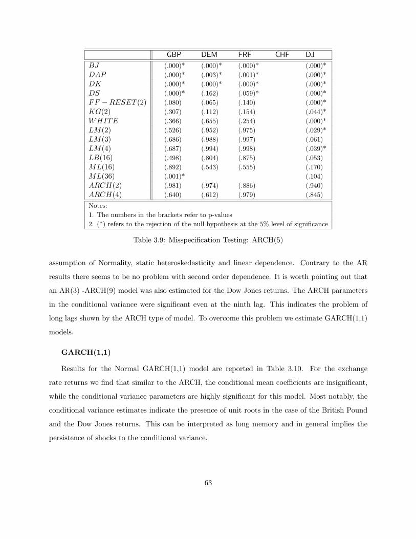
GBP DEM FRF CHF DJ
BJ (.000)* (.000)* (.000)* (.000)*
DAP (.000)* (.003)* (.001)* (.000)*
DK (.000)* (.000)* (.000)* (.000)*
DS (.000)* (.162) (.059)* (.000)*
FF −RESET (2) (.080) (.065) (.140) (.000)*
KG(2) (.307) (.112) (.154) (.044)*
WHITE (.366) (.655) (.254) (.000)*
LM(2) (.526) (.952) (.975) (.029)*
LM(3) (.686) (.988) (.997) (.061)
LM(4) (.687) (.994) (.998) (.039)*
LB(16) (.498) (.804) (.875) (.053)
ML(16) (.892) (.543) (.555) (.170)
ML(36) (.001)* (.104)
ARCH(2) (.981) (.974) (.886) (.940)
ARCH(4) (.640) (.612) (.979) (.845)
Notes:
1. The numbers in the brackets refer to p-values
2. (*) refers to the rejection of the null hypothesis at the 5% level of significance
Table 3.9: Misspecification Testing: ARCH(5)
assumption of Normality, static heteroskedasticity and linear dependence. Contrary to the AR
results there seems to be no problem with second order dependence. It is worth pointing out that
an AR(3) -ARCH(9) model was also estimated for the Dow Jones returns. The ARCH parameters
in the conditional variance were significant even at the ninth lag. This indicates the problem of
long lags shown by the ARCH type of model. To overcome this problem we estimate GARCH(1,1)
models.
GARCH(1,1)
Results for the Normal GARCH(1,1) model are reported in Table 3.10. For the exchange
rate returns we find that similar to the ARCH, the conditional mean coefficients are insignificant,
while the conditional variance parameters are highly significant for this model. Most notably, the
conditional variance estimates indicate the presence of unit roots in the case of the British Pound
and the Dow Jones returns. This can be interpreted as long memory and in general implies the
persistence of shocks to the conditional variance.
63
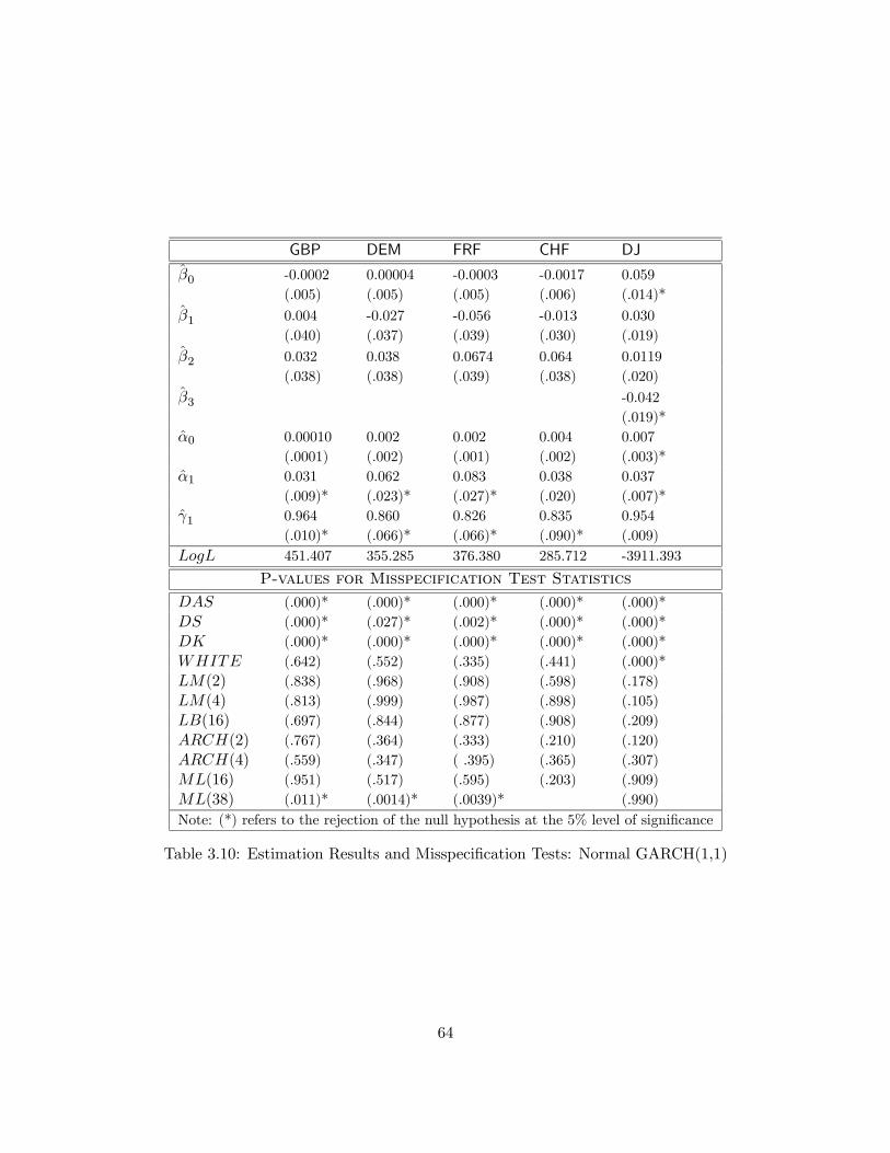
GBP DEM FRF CHF DJ
β0 -0.0002 0.00004 -0.0003 -0.0017 0.059
(.005) (.005) (.005) (.006) (.014)*
β1 0.004 -0.027 -0.056 -0.013 0.030
(.040) (.037) (.039) (.030) (.019)
β2 0.032 0.038 0.0674 0.064 0.0119
(.038) (.038) (.039) (.038) (.020)
β3 -0.042
(.019)*
α0 0.00010 0.002 0.002 0.004 0.007
(.0001) (.002) (.001) (.002) (.003)*
α1 0.031 0.062 0.083 0.038 0.037
(.009)* (.023)* (.027)* (.020) (.007)*
γ1 0.964 0.860 0.826 0.835 0.954
(.010)* (.066)* (.066)* (.090)* (.009)
LogL 451.407 355.285 376.380 285.712 -3911.393
P-values for Misspecification Test Statistics
DAS (.000)* (.000)* (.000)* (.000)* (.000)*
DS (.000)* (.027)* (.002)* (.000)* (.000)*
DK (.000)* (.000)* (.000)* (.000)* (.000)*
WHITE (.642) (.552) (.335) (.441) (.000)*
LM(2) (.838) (.968) (.908) (.598) (.178)
LM(4) (.813) (.999) (.987) (.898) (.105)
LB(16) (.697) (.844) (.877) (.908) (.209)
ARCH(2) (.767) (.364) (.333) (.210) (.120)
ARCH(4) (.559) (.347) ( .395) (.365) (.307)
ML(16) (.951) (.517) (.595) (.203) (.909)
ML(38) (.011)* (.0014)* (.0039)* (.990)
Note: (*) refers to the rejection of the null hypothesis at the 5% level of significance
Table 3.10: Estimation Results and Misspecification Tests: Normal GARCH(1,1)
64

In terms of misspecifications, the Normal GARCH models suffer from excess kurtosis and skew-
ness and thus violate the Normality assumption. The ML statistics suggest some dynamic mis-
specification in the case of the British pound, the Deutschemark and the French Franc. In some
sense misspecifications are more pronounced here than in the Normal ARCH case. The results for
Dow Jones returns indicate that only the third lag in the conditional mean is significant. In terms
of misspecifications it seems that the GARCH(1,1) is performing better than the ARCH but still
exhibits problems with Normality and static heteroskedasticity. Next we change the distribution
assumption to Student’s t and estimate Bollerslev’s Student’s t GARCH (1987).
Student’s t GARCH
The estimated parameters and the relevant misspecification tests are shown in Table 3.11. The
estimated conditional mean parameters are all insignificant as in the case of the Normal GARCH
model. Note that the conditional mean estimates are similar in magnitude to the OLS, ARCH
and GARCH estimates. Misspecification tests indicate that despite the adoption of the Student’s
t distribution this formulation still suffers from skewness and excess kurtosis2. The next model
based on the PR approach addresses these issues systematically.
2Recall that excess kurtosis is an inherent feature of the Student’s t distribution.
65

GBP DEM FRF CHF DJ
β0 0.044 0.014 -0.017 -0.0005 0.076
(.043) (.062) (.099) (.006) (.013)*
β1 -0.011 -0.024 -0.042 -0.002 0.010
(.044) (.035) (.041) (.031) (.017)
β2 0.035 0.075 0.072 0.069 -0.027
(.036) (.037)* (.038) (.037) (.017)
β3 -0.049
(.017)*
α0 0.029 0.165 0.172 0.003 0.006
(.019) (.100) (.108) (.002) (.002)*
α1 0.044 0.058 0.073 0.041 0.038
(.015)* (.023)* (.029)* (.021) (.008)*
γ1 0.939 0.872 0.850 0.866 0.956
(.021)* (.056)* (.067)* (.074)* (.009)*
ν 7.289 9.664 8.997 9.333 5.061
(1.581)* (2.803)* (2.513)* (2.702)* (0.474)
LogL -839.625 -949.517 -927.142 729.81
P-values for Misspecification Test Statistics
DAS (.000)* (.000)* (.000)* (.000)* (.000)*
DS (.000)* (.028)* (.003)* (.200) (.000)*
DK (.000)* (.000)* (.000)* (.000)* (.000)*
WHITE (.734) (.554) (.333) (.468)
AC(2) (.794) (.976) (.960) (.656)
AC(4) (.789) (.999) (.993) (.921)
LB(16) (.703) (.847) (.898) (.916)
ARCH(2) (.755) (.366) (.325) (.245)
ARCH(4) (.693) (.344) (.372) (.397)
ML(16) (.987) (.560) (.571) (.242)
Note:
1. (*) refers to the rejection of the null hypothesis at the 5% level of significance
Table 3.11: Estimation Results and Misspecification Tests: Student’s t GARCH
66

Student’s t Autoregressive models with dynamic heteroskedasticity
The probabilistic features of the data in hand, point to the direction of a Student’s t Autore-
gressive model as a convenient framework for analyzing both the temporal dependence and the
leptokurtosis. We now provide a formal illustration of the PR methodology by presenting the re-
sults from this model in Table 3.12. Note that the misspecification tests presented in Table 3.12
are based on the weighted residuals3 proposed by Spanos (1990).
A STAR(2,2,9) model was found to be statistically adequate for the Deutschemark and the
Swiss Franc, while a STAR(2,2,8) was required for the French Franc. The British Pound was
best described by a STAR(2,2,5). To get a statistically adequate model for the British Pound we
“dummy” the observation for “Black Wednesday”. It is also interesting to note that the estimates
of the conditional mean differ in magnitude from those obtained using the OLS, ARCH, and the
Normal GARCH specifications. However they are much closer to the Student’s t GARCH. This
can perhaps be explained by the fact that the data looks much closer to the Student’s t distribution
rather than the Normal. For the Dow Jones a STAR(3,3,4) was found to be statistically adequate.
Compared to the Normal GARCH we observe that misspecification tests suggest no problems with
static heteroskedasticity in this case.
3The weighted residuals are defined as . utωt− ωtεt, where ut = yt − β0 +
lPi=1
βiyt−i, and εt ∼ St(0, 1; ν) is a
simulated standard i.i.d. Student’s t series. These residuals are a modification of the usual (Pearson) residuals,where the additional term purports to account for the non-linear effects of the conditional variance on yt.
67

GBP(ν = 5) DEM(ν = 9) FRF(ν = 8) CHF(ν = 9) DJ(ν = 4)
β1 0.0050 -0.0070 -0.0199 0.0074 0.028
(.026) (.0411) (.043) (.037) (.023)
β2 0.0524 0.0731 0.0755 0.0702 -0.022
(.0391) (.0404) (.039) (.039) (.034)
β3 -0.052*
(.020)
q0 0.1970 0.1096 0.1235 0.1092 0.249
(.012)* (.006)* (.007)* (.006)* (.005)*
q1 0.002 0.0017 0.004 -0.000068 -.007
(.006)* (.004) (.005) (.005) (.005)
q2 -0.0117 -0.0097 -0.0109 -0.0093 0.004
(.008) (.005)* (.005)* (.005)* (.005)
q3 -0.006
(.005)
σ2 0.9527 1.6073 1.451 0.485
(.061)* (.094)* (.086)* (.029)*
LogL -1,396 -1,379 -930
P-values for Misspecification Test Statistics
DS (.000)* (.414) (.066) (.40) (.021)*
DK (.000)* (.000)* (.000)* (.000)* (.000)*
WHITE (.201) (.800) (.180) (.280) (.944)
LM(2) (.345) (.860) (.549) (.600) (.668)
LM(4) (.431) (.955) (.534) (.336) (.298)
LB(16) (.500) (.970) (.408) (.740) (.710)
ARCH(2) (.433) (.607) (.640) (.580) (.302)
ARCH(4) (.500) (.565) ( 650) (.745) (.286)
ML(26) (.450) (.987) (.720) (.730) (.292)
ML(38) (.54) (.640) (.80) (.760) (.757)
Note: (*) refers to the rejection of the null hypothesis at the 5% level of significance
Table 3.12: Estimation Results and Misspecification Tests: Student’s t AR Models
68

3.5 Conclusion
In this chapter we illustrate the use of graphical techniques for identifying chance regularity patterns
in the data and guiding us to a valid specification for exchange rate volatility. In view of the
preliminary data analysis, Normality was rejected as being inappropriate for this data. Also the
presence of second order dependence and leptokurtosis suggested that the Student’s t distribution
was likely to be more appropriate. This gave rise to the Student’s t autoregressive formulation for
modeling speculative prices which directly takes into account the nature of the data. An important
aspect of the graphical techniques is the creative use of the P-P plots which provide a reasonably
good approximation for the actual degrees of freedom involved.
The empirical analysis of this chapter shows that the Student’s t Autoregressive model provides
a parsimonious account of the probabilistic features of the exchange rate data. Furthermore, mis-
specification testing reveals that the Student’s t AR specification outperforms the GARCH type
formulations on statistical adequacy grounds. Estimation results suggest that there are substantial
similarities in the movements of European exchange rate returns which indicate the necessity of
the multivariate framework. Moreover the well specified univariate volatility models seem to share
similar degrees of freedom thus allowing us to explore the possibility of the Student’s t VAR model.
Finally this chapter illustrates that the PR approach provides a systematic technique for for-
mulating well specified models. Its comprehensive toolkit consisting of graphical techniques and
the systematic reduction leads to an internally consistent statistical model. This gives us confi-
dence that we can extend the univariate Student’s t AR formulation to the multivariate framework
without having to resort to ad hoc restrictions and contradictory assumptions.
69

Chapter 4
Degrees of Freedom, Sample Kurtosis
and the Student’s t GARCH Model
In this chapter we make a digression from the central theme of the dissertation −modeling volatility− to examine certain interesting side issues. As shown in Chapter 2 there is plenty of evidence in theliterature that points to leptokurtosis and the presence of second order dependence in economic and
financial data. Using plots of financial data, in Chapter 3, we find that the Student’s t distribution
provides a better description of this type of data.
Econometric modeling based on the Student’s t distribution introduces an additional parameter
− the degree of freedom parameter, which measures the extent of leptokurtosis in the data. One
can also interpret this as a measure of the extent of departure from the Normal distribution. Two
questions naturally arise at this stage in the context of the Student’s t distribution. The first one
relates to using the sample kurtosis coefficient for determining the appropriate degree of freedom
parameter. The second question is concerned with the reliability of the estimated degree of freedom
parameter from Bollerslev’s (1987) Student’s t GARCH model. In this chapter a simulation study
was performed to investigate these questions.
In the next section we describe the design of the simulation set up. Section 4.2 presents the
analysis of results. The final section has some concluding remarks.
70

4.1 Simulation Set Up
We begin by providing a formal description of the two questions of interest. Next we describe the
simulation design to study these questions.
4.1.1 Theoretical Questions
The sample kurtosis coefficient defined as α4 = 3 +6
ν−4 provides one way of choosing the degrees
of freedom parameter ν for the Student’s t distribution. Despite its popularity, the sample kurtosis
coefficient − the standardized fourth central moment has been criticized a lot in the in the statisticsliterature as a “vague concept”(Mosteller and Tuckey, 1977). Also Ballanda and MacGillivray
(1988) point out that “although moments play an important role in statistical inference they are
very poor indicators of distributional shape”. Given these criticisms it is not apparent that the
kurtosis coefficient is a useful way to compute the implied degrees of freedom. Hence we use a
simulation study to investigate the sampling distribution of the kurtosis coefficient and the sampling
distribution of the implied degrees of freedom parameter.
The second objective of this simulation study is to examine the reliability of the estimated
degrees of freedom parameter from the Student’s t GARCH model. Bollerslev (1987) introduced
the Student’s t GARCH model by suggesting the following distribution of the error term
f(ut/Ypt−1; θ1) =
Γ£12 (ν + 1)
¤π12Γ£12ν¤ £
(ν − 2)h2t¤− 1
2
·1 +
u2t(ν − 2)h2t
¸− 12(ν+1)
(4.1)
Recall from Chapter 2 that h2t is the GARCH formulation of the conditional variance and can
be written as follows:
h2t = ω +
pXi=1
aiu2t−i +
qXj=1
γjh2t−j , p ≥ 1, q ≥ 1 (4.2)
where the parameter restrictions ω > 0, ai ≥ 0, γj ≥ 0 ensure that the conditional variance is
always positive. As beforepPi=1ai +
qPj=1
γj < 1 is required for the convergence of the conditional
variance.
71

McGuirk et al. (1993) point out that the above distribution in equation (4.1) can be obtained
by substituting the conditional variance h2t in the functional form of the marginal Student’s t
distribution and re-arranging the scale parameter. This would be indeed the correct strategy for
the Normal distribution, since one does not have to be concerned about the degree of freedom
parameter. In the case of the Student’s t distribution however, the degrees of freedom in the
conditional distribution change depending on the number of the conditioning variables. In fact
McGuirk et al. (1993) further show that if we derive the conditional distribution from the joint
distribution of the observables f(yt, yt−1,...yt−p;ψ) we get the expression shown in equation (4.3)
below:
f(ut/Ypt−1; θ2) =
Γ£12 (ν + p+ 1)
¤π12Γ£12ν + p
¤ £νσ2h2t
¤− 12
·1 +
u2tνσ2h2t
¸− 12(ν+p+1)
(4.3)
Note that the parameter in the gamma function in the two equations are different. More
importantly however, we observe that σ2 does not appear in equation (4.1). This suggests that
estimation of the degree of freedom parameter, ν from the Student’s t GARCH model ala Bollerslev
(1987), that ignores σ2 will give an incorrect mixture of both ν and σ2. To investigate this issue
further we allow σ2 to vary and examine its effect on all estimated parameters from the Student’s
t GARCH model.
4.1.2 Data Generation
This simulation study uses a program developed by Paczkowski (1997)1. The data for this sim-
ulation were generated in the following way. First, a raw series of Student’s t random numbers
with mean 0 and variance 1 is generated. The degree of freedom parameter was allowed to vary in
different simulations according to the needs of the study. The true structure of the data is given
by:
Y1t ∼ Stt
¡1tµ,Σ
1t , ν¢, t = 1, . . . , T,
1By running a series of Monte Carlo experiments Paczkowski (1997) investigates the usefuleness of the Student’st regression models for estimation and testing, and their ability to capture dynamic heteroskedasticity.
72

where Y1t = (Y1, Y2, . . . , Yt)
0 , µ = 0, and (Σ1t )−1 is
(Σ1t )−1 =
1 −0.4 −0.2−0.4 1.16 −0.32 −0.2−0.2 −0.32 1.20 −0.32 −0.2
−0.2 −0.32 1.20 −0.32 −0.2. . . .
. . . .
−0.2 −0.32 1.20 −0.32 −0.20−0.2 −0.32 1.16 −0.4
−0.2 −0.4 1
(4.4)
Using µ = 0 and equation (4.4) the remaining parameters can be computed as follows:
β =
β2
β1
=
0.2
0.4
, σ2 = 1, β0 = 0.
Next, we use the Cholesky factorization as shown below to impose the necessary dependence
structure on the generated data.
Y1T = chol
µν
ν − 2Σ1T
¶J (4.5)
where J is the series of raw Student’s t numbers and Σ1T is the scale matrix, and chol(.) refers to
the Cholesky factorization.
The raw Student’s t numbers were generated using the algorithm proposed by Dagpunar (1988).
This algorithm uses numbers from a uniform distribution as an input, allowing the user to control
the seed. The following procedure was chosen in order to enable easy reproduction of the data
from any given run. First the initial seed was set to 211− 1 and series of Student’s t numbers weregenerated. The generated data were tested for skewness and kurtosis using tolerance levels used
in Paczkowski (1997). Only samples that met the standards were used in the simulation study.
73
Maximum allowable skewness was set to ±0.1. The tolerance for kurtosis was set to ±0.5 aroundthe value implied by the degree of freedom parameter according to the relationship shown below:
α4 = 3 +6
ν − 4; ν > 4 (4.6)
Note that for ν = 4 the above relationship breaks down and the allowable kurtosis range was set
to 7.5−8.5.
To study the questions of interest discussed in Section 4.1.1 we consider a number of different
scenarios. Sample sizes (n) of 50, 100, 500 and 1000 were chosen since financial data series can be
available annually, monthly, weekly or daily. Three different degrees of freedom ν = 4, 6, and 8
were used in this study. The true value of α4 is 6 when ν = 6 and 4.5 when ν = 8. For ν = 4 α4
is undefined. Most financial data are leptokurtic and thus can be described by degrees of freedom
in the range of 4−8. Also as ν increases above 8 the distribution looks much closer to the Normal.Hence it would be uninteresting to consider larger degrees of freedom. For each combination of the
sample size and ν, 1000 data sets were generated. Also for sample size 500 we allowed σ2 to vary.
It took the values 1, 0.25 and 4. In each of these instances the value of σ2 affects only the scale
matrix Σ1t , leaving the other parameters unchanged. For σ2 = 1, (Σ1t )
−1 takes the values given in
equation (4.3). In general for σ2 = k, k > 0, the inverse of the scale matrix in equation (4.3) is
multiplied by the factor of 1k .
The computer code for this simulation exercise was written in GAUSS 4.0 and the Student’s t
GARCH model was estimated using the FANPAC toolbox which is part of the GAUSS package.
4.2 Results
In this section we present the results of the simulation study. In the first part we present the
results for the sample kurtosis coefficient α4 and the implied degrees of freedom parameter (inu)
computed using α4. In the second part we focus on the degrees of freedom parameter as estimated
in Bollerslev’s (1987) model. By allowing σ2 to take different values we examine its impact on all
estimated parameters.
74

Parameter DF Sample size Mean Empirical s.e Skewness Kurtosis
ν = 4
50
100
500
1000
5.2981
5.5234
5.6626
5.6577
.9064
.9170
.6454
.5183
.4637
.3247
.6828
.6625
3.2697
3.0346
4.3656
4.4543
α4 ν = 6
50
100
500
1000
4.3069
4.4364
4.5507
4.5317
.7529
.7100
.4824
.3960
.5666
.5382
.5406
.5921
3.7797
3.7072
3.6502
3.3306
ν = 8
50
100
500
1000
3.6416
3.7211
3.7202
3.7350
.6341
.5630
.3554
.2914
.4985
.6295
.7278
.7100
3.2237
3.7385
4.0377
4.0557
ν = 4
50
100
500
1000
6.7046
6.8047
6.3920
6.3441
10.0026
2.0034
.6194
.4664
-20.6339
2.8237
1.3633
.9253
458.6991
95.6585
7.1254
5.5797
inu ν = 6
50
100
500
1000
10.3436
14.6619
8.3120
8.1886
21.9843
145.1031
1.6467
1.1193
-.2979
30.0049
2.4282
0.9077
74.1571
929.4971
14.7343
4.2954
ν = 8
50
100
500
1000
-1.4269
992.27.62
15.5592
13.1225
314.2906
30878
26.7089
25.5438
-22.8729
31.5739
6.0128
-28.1416
631.6351
997.9412
316.9994
864.1377
Table 4.1: Descriptive Statistics for Sample Kurtosis and inu
4.2.1 Estimates of α4 and the Implied Degrees of Freedom
In Table 4.1 we report descriptive statistics for the empirical distribution of the estimates. We
observe that the sample kurtosis coefficient, α4 is relatively stable around 5.6 for ν = 4. Similarly it
is stable around 4.5 for ν = 5, and around 3.7 for ν = 6. Also note that as ν increases, α4 decreases
as expected. However, once we use α4 to derive the implied degrees of freedom (inu), we find some
interesting features. In all three cases (ν = 4, 6, 8) the implied degrees of freedom consistently
exceeds the true ones. For ν = 4, inu is around 6 (starting at 6.7 for sample size of 50 and going
down to 6.3 for sample size of 1000). Also note that the standard error decreases dramatically from
a value of 10 (n = 50) to a value of 0.46 (n = 1000). For ν = 6, at sample size 50, inu = 10, but
75

stabilizes around 8 for sample sizes 500 and 1000. Interestingly for sample size 100 it jumps to 14
and the standard error is high as well. For ν = 8 we find evidence of erratic behavior especially
for sample sizes of 50 and 100 where inu = −1.4 and inu = 992 respectively. As the sample sizeincreases the implied degrees of freedom parameter decreases to 13 for n = 1000 and possibly could
decrease even more for sample sizes beyond 1000. This erratic behavior at small sample sizes can
largely be explained by the fact that a few bad draws can affect the (mean) estimates for small
sample sizes. Also as mentioned before, for ν = 6 and ν = 8, we find that α4 is around 4 and 3
respectively. Recall that inu = 4 + 6α4−3 . Hence for ν = 6 and ν = 8 there is a higher probability
of getting unusually large values for inu. This can explain the erratic behavior observed above.
Overall, the results suggest that the sample kurtosis coefficient is not a good measure of the true
degrees of freedom.
4.2.2 Estimates of the Student’s t GARCH parameters
Table 4.2 provides descriptive statistics for the empirical distribution of the degree of freedom
parameter (nu), estimated by Bollerslev’s (1987) model. The results suggest that the Student’s
t GARCH model consistently overestimates the true degree of freedom parameter. For instance
when ν = 4, the estimated value is around 8. Also note that for small sample sizes the empirical
standard error of the parameters is larger than their estimated value. Even if sample size increases
the standard error is quite large giving rise to imprecise estimates. For ν = 4 estimated nu is stable
around the value of 8. For ν = 6 and ν = 8 as the sample size increases we observe a downward
trend towards the true value of ν, although the final estimates are nowhere close to it.
Next we present Table 4.3 which shows how the estimates of the conditional variance from the
Student’s t GARCH model vary for different values of σ2. We chose to use a sample size of 500 in
this case to avoid any problems with small sample sizes. Recall that σ2 is not a free parameter to
be estimated in Bollerslev’s (1987) formulation (see equation 4.1). Therefore we can interpret this
as the σ2 = 1 case, that serves as the benchmark. Interestingly, we find that the only parameter
which varies with σ2 is ω − the constant term in the conditional variance equation. Moreover, we
observe that there is an approximate relationship between σ2and ω. For example when ν = 4 and
σ2 = 4 the estimate of ω is 4.5016 which is roughly four times the value of ω when σ2 = 1. This
76

Parameter DF Sample size Mean Empirical s.e Skewness Kurtosis
ν = 4
50
100
500
1000
7.8161
8.2640
7.9918
8.1036
12.4646
10.9403
2.7387
1.8096
5.2276
5.3855
3.0789
1.8848
31.7047
35.1996
22.0161
9.4895
nu ν = 6
50
100
500
1000
13.0683
12.2761
10.9033
11.0866
20.7030
16.1543
4.1220
2.8603
3.0020
3.5597
1.9758
1.2313
10.9406
15.7681
8.9713
5.0127
ν = 8
50
100
500
1000
20.7026
20.3718
17.7961
15.4479
27.1638
24.1092
10.3940
4.5214
1.8269
2.0239
2.9042
1.9255
4.9891
6.0065
16.7992
13.8620
Table 4.2: Descriptive Statistics for Estimated nu
relationship holds for ν = 6, 8 (see Table 4.4). We can also see from Table 4.3 that the estimated
degree of freedom (nu), and the GARCH and ARCH parameters in the conditional variance remain
unchanged as σ2 varies.
These results suggest that the effect of the σ2 (the missing parameter) in Bollerslev’s formulation
is fully absorbed by the constant in the conditional variance equation.
We also present Normal kernel density estimates of the empirical distribution of nu for various
sample sizes and ν = 6 in Figures 4—1− 4-6. Graphs for ν = 4 and ν = 8 exhibit similar patterns.
The dashed lines in the pictures represent the contour of the Normal density, with the same mean
and variance as the data whose distribution is shown in the graph. The pictures in Figure 4—1 −4-6 indicate that the distribution is skewed to the left and the mode and the mean are far from the
true value (ν = 6). The graphs also show strong evidence of leptokurticity.
77

Parameter DF σ2 Mean Empirical s.e Skewness Kurtosis
nu ν = 41
0.25
4
7.9918
7.8868
7.8574
2.7387
2.5311
2.5787
3.0789
3.0377
3.2067
22.0161
24.2803
27.3063
ω ν = 41
0.25
4
1.1164
.2778
4.5016
.3846
.0959
1.5929
.4161
.3616
.4569
3.1568
3.0933
3.1791
γ1 ν = 41
0.25
4
.2226
.2264
.2196
.2074
.2072
.2121
-.0394
.0119
-.0699
2.8308
2.8227
2.8588
a1 ν = 41
0.25
4
.2229
.2219
.2219
.0642
.0642
.0641
.3804
.3653
.3451
3.2621
3.1943
3.0918
Note:
1. γ1 is the GARCH parameter, a1 is the ARCH parameter and ω is the constantin the Student’s t GARCH model (Bollerslev, 1987)
Table 4.3: Descriptive Statistics for the Student’s t GARCH parametes, n=500
Parameter DF σ2 Mean Empirical s.e Skewness Kurtosis
ω ν = 41
0.25
4
1.1164
.2778
4.5016
.3846
.0959
1.5929
.4161
.3616
.4569
3.1568
3.0933
3.1791
ω ν = 61
0.25
4
.9111
.2246
3.6325
.4027
.0987
.1896
.6434
.5478
.5383
4.0782
3.6875
3.7684
ω ν = 81
0.25
4
.9728
.2454
3.8037
.5244
.1310
2.0297
.7333
.7034
.6705
3.2792
3.2997
3.2348
Table 4.4: Descriptive Statistics for the constant in the Student’s t GARCH model, n=500
78

Figure 4-1: Kernel density for nu, ν = 6, σ2 = 1, n = 50
Figure 4-2: Kernel density for nu, ν = 6, σ2 = 1, n = 100
79

Figure 4-3: Kernel density for nu, ν = 6, σ2 = 1, n = 500
Figure 4-4: Kernel density for nu, ν = 6, σ2 = 1, n = 1000
80

Figure 4-5: Kernel density for nu, ν = 6, σ2 = 0.25, n = 500
Figure 4-6: Kernel density for nu, ν = 6, σ2 = 4, n = 500
81

4.3 Conclusion
In this chapter we investigate some interesting side questions relating to the degree of freedom
parameter in the Student’s t distribution. In particular we have focused on: (i) the ability of the
kurtosis coefficient to accurately capture the implied degrees of freedom and (ii) the ability of Stu-
dent’s t GARCH model to estimate the true degree of freedom parameter accurately. With regard
to the first question the simulation study reveals that the kurtosis coefficient provides a biased and
inconsistent estimator of the degree of freedom parameter. With regard to the second question,
our findings can be summarized as follows. First, the simulation results show that the Student’s t
GARCH model provides a biased and inconsistent estimator of the degree of freedom parameter.
More importantly however, when σ2 is allowed to vary the constant term in the conditional variance
equation is the only parameter that is affected. The conditional mean parameters along with the
ARCH and GARCH coefficients and the degree of freedom parameter are not affected by varying
σ2.
82
Chapter 5
Student’s t Dynamic Linear
Regression
Until now we have considered models of univariate volatility involving only the past history of the
series itself to explain volatility. In fact Pagan (1996) claims that a purely statistical approach has
dominated the univariate modeling of financial data. However, in recent years it has been pointed
out in the literature that other exogenous variables might also be responsible for volatility. Granger
(2002) suggests that “volume or perhaps daily trade would be interesting explanatory variables to
include in a model of volatility particularly as both of these variables appear to be forecastable”.
Along the same lines Engle and Patton (2001d) point out: “Of course no-one believes that financial
asset prices evolve independently of the market around them, and so we expect that other variables
may contain relevant information for the volatility of the series”. Evidence in this direction can
be found in earlier papers by Engle et al. (1990b), Engle and Mezrich (1996), and Bollerslev and
Melvin (1994b). Glosten, Jagannathan and Runkle (1993) also find evidence that indicator variables
can help to explain dynamic conditional volatility of equity returns. Moreover deterministic events
such as macroeconomic announcements and scheduled company announcements are also believed
to have an influence on volatility. For example Andersen and Bollerslev (1998) find that volatility
of the Deutschemark-Dollar exchange rate increases around the time of announcements of US
macroeconomic data such as the quarterly GDP and the Producer Price Index. Although the
literature has recognized the importance of exogenous variables in explaining volatility, very little
83

work has been done to explore this issue. This is primarily because the GARCH framework models
volatility through the error term making it hard to justify the inclusion of other contemporaneous
variables.
The primary objective of this chapter is to develop a Student’s t Dynamic Linear Regression
(DLR) model for univariate volatility in terms of the volatility of the series itself, as well as other
relevant exogenous variables. We illustrate this approach by using two different exchange rate
returns data sets and a data set which consists of daily returns of the Dow Jones Industrial Price
index and the Three -month treasury bill rate.
In the next section we introduce some notation and develop the specification of the Student’s t
DLR model. We also discuss the maximum likelihood estimation of this model. In Section 5.2 we
provide the empirical results. The estimated Student’s t DLR model is compared to the traditional
Normal DLR, the Student’s t AR and the Normal GARCH−X (which allows for exogenous variablesin the conditional variance). Finally in Section 5.3 we conclude by summarizing the empirical results
and their implications.
5.1 Student’s t DLR Model
5.1.1 Specification
In the context of the Probabilistic Reduction approach, the operational Student’s t DLR model is
specified by imposing certain reduction assumptions on the joint distribution of the vector stochastic
process Zt, t ∈ T where Zt ≡ (yt,x0t)0. Here yt is the dependent variable and xt is a (k × 1) vectorof exogenous variables. The reduction assumptions are derived from the probabilistic features of the
underlying stochastic process and as before can be summarized into three categories: Distributional
assumption, Dependence and (time) Heterogeneity assumptions. For the Student’s t DLR model
the reduction assumptions are given by:
1. Distribution: Student’s t
2. Dependence: Markov of order p
3. Heterogeneity: Second Order Stationarity
84

Using these assumptions the reduction can be performed in the following way:
D(Z1,Z2,Z3, ...ZT ;ψ(t)) = D1(Z1;ϕ1)TQt=2D(Zt | Zt−1,Zt−2, ...Z1;ϕ(t))
M(p)= D(Zp;ϕ1(t))
TQt=p+1
D(Zt | Zt−1,Zt−2, ...Zt−p;ϕ2(t))
= D(Zp;ϕ1(t))TQ
t=p+1D(Zt | Zt−pt−1;ϕ2(t))
SS= D(Zp;ϕ1)
TQt=p+1
D(Zt | Zt−pt−1;ϕ2)
= D(Zp;ϕ1)TQ
t=p+1D(yt | Zt−pt−1 xt; θ1)D(xt | Zt−pt−1; θ2)
(5.1)
where Zt−pt−1 :=¡Zt−1,Zt−2, ...,Zt−p
¢denotes the past history of Zt and Zp ≡
¡Z1, . . . ,Zp
¢denotes
the initial conditions. Also ψ(t), ϕ1, and ϕ2 denote the parameters in the joint, marginal and
conditional distributions respectively. The first equality shows that the joint distribution can be
decomposed into a product of (T −1) conditional distributions and one marginal distribution. Theassumption of Markov(p) changes the conditioning information set to
¡Zt−1,Zt−2, ...,Zt−p
¢. This
allows us to have an information set that can be handled more easily since it depends only on the
past p periods. The third equality shows that under the assumption of second order stationarity,
the statistical parameters ϕ1 and ϕ2 are time invariant. This leads to a reduction in the number
of unknown parameters. In the last equality we simply decompose Zt into (yt,x0t)0. Taken together
these assumptions allow us to express the Student’s t DLR model in terms of the first two moments
as shown in the next page.
85
The Student’s t Dynamic Linear Regression Model
[A] The conditional mean takes the form:
yt = β00xt +pXi=1
αiyt−i +pXi=1
β0ixt−i + ut, t ∈ T (5.2)
where ut = yt −E(yt|Ft−1) is distributed St(0, h2t ; ν), and Ft−1 = σ(Y0t−1),X0
t = x0t .
Y0t−1 ≡ (yt−1 , yt−2, . . . , y1), and X0t ≡ (xt,xt−1, . . . ,x1).
[B] The conditional variance, h2t is given by:
h2t ≡·
υ
ν + k1− 2¸σ2£1 + (X∗t −M∗
t )0Σ−122 (X
∗t −M∗
t )¤, (5.3)
where X∗t = (x0t, yt−1, . . . yt−p,x0t−1, . . .x0t−p)0,M∗t = (µ
0x, µy1t−p, µx1t−p)0, are both (k1×1) vectors
and k1 = k(p + 1) + p is the number of conditioning variables and Σ22 is the variance-covariance
matrix of X∗t .
The Student’s t DLR can be fully specified as shown in Table 5.1.
86

The Student’s t Dynamic Linear Model
I. Statistical GM: yt = β00xt +pPi=1
αiyt−i +pPi=1
β0ixt−i + ut, t > p.
[1]Dt = Z0t−1,Xt is the relevant conditioning information set withµt = E(yt | σ(Y0
t−1),X0t = x
0t ) = β00xt +
pPi=1
αiyt−i +pPi=1
β0ixt−i : the systematic component,
and ut = yt −E(yt | σ(Y0t−1),X0
t = x0t ) : the non-systematic component.
[2]θ∗ := (α1,α2, . . . ,αp,β0,β1,...βp,σ2,Σ−122 ), are the statistical parameters of interest,
[3]The parameters α ≡ (α1,α2, . . . ,αp)0 satisfy the restriction that all the roots of the polynomial(λp −
pPi=1
αiλp−i) = 0 are less than one in absolute value.
[4]No a priori restrictions on θ∗ := (α1,α2, . . . ,αp,β0,β1,...βp,p,σ2,Σ−122 )
[5]Rank(X∗) = k(p+ 1) + p for all the observable values of Y0t−p, T > k(p+ 1) + p.
II. Probability model: Φ =©D(yt | σ(Yt−1),X0
t = x0t ;θ
∗), Zt ∈ Rmª.
[6]
(i) D(yt | σ(Yt−1),X0
t = x0t ;θ
∗) is Student’s t,(ii) E(yt | σ(Y0
t−1),X0t = x
0t ;θ
∗) = β∗X∗t is linear in X∗t ,
(iii)V ar(yt | σ(Y0
t−1),X0t = x
0t ) =h
νν+k1−2
iσ2£1 + (X∗t −M∗
t )0Σ−122 (X
∗t −M∗
t )¤is heteroskedastic.
[7]The parameters ϕ are t-invariant.
III. Sampling model:[8]y ≡ (yp+1, yp+2, . . . , yT ) is stationary asymptotically independent sample sequentiallydrawn from D(yt | σ(Z0t−1),X0
t = x0t ;θ
∗), t = p+ 1, p+ 2, . . . , T, respectively.
Table 5.1: The PR Approach: Student’s t DLR Specification
It is also interesting to see how the reduction assumptions relate to the probabilistic assump-
tions of the Student’s t DLR model. Observe that in Table 5.2 the conditional mean is linear
in the conditioning variables as in the case of Normal DLR model. (For details on the Normal
DLR see Spanos (1986)). The assumption of Student’s t however leads to a conditional variance
function which is different from that of the Normal DLR model. It accommodates both static and
dynamic heteroskedasticity. In particular static heteroskedasticity enters the conditional variance
specification through the presence of contemporaneous variables, and dynamic heteroskedasticity
enters through the lags of the conditioning variables. We now discuss the estimation of this model.
87

Reduction Assumptions: Model Assumptionsyt, t ∈ T (yt | σ(Y 0t−1),X0
t = x0t ; θ
∗), t ∈ T
Student’s t −→(i) D(yt | σ(Y 0t−1),X0
t = x0t ; θ
∗) is Student’s t(ii) E(yt | σ(Y 0t−1),X0
t = x0t ; θ
∗) = β∗X∗t is linear in X∗t(iii) Cov(yt | σ(Y 0t−1),X0
t = x0t ; θ
∗) = h2t is heteroskedastic,
Markov −→ ¡ut | σ(Y0t−1),X0
t = x0t
¢, t ∈ T
is a martingale difference process
Stationarity −→ The parameters θ∗ := (α1,α2, . . . ,αp,β0,β1,...βp, σ2,Σ−122 )
are t-invariant.
Table 5.2: Reduction and Probability Model Assumptions: Student’s t DLR
5.1.2 Maximum Likelihood Estimation
To estimate the Student’s t DLR model typically one should substitute the functional form of
D(yt | Zt−pt−1 Xt;ϕ2) and D(Xt | Zt−pt−1;ϕ3) in equation (5.1) to obtain the likelihood function of the
Student’s t DLR model. The logarithmic form of the likelihood function can then be differentiated
to obtain the first order conditions. These can be solved to get the estimators of the parameters
of interest. However, instead of following this approach we use an easier technique based on the
reparametrization of the joint density. When Zt is distributed multivariate Student’s t its density
takes the form:
D(Zt) =Γ£12 (ν + k1 + 1)
¤(πν)
k1+12 Γ
£12 (ν)
¤ (detΣ)−12
·1 +
1
ν(Zt − µ)0Σ−1 (Zt − µ)
¸ 12(ν+k1+1)
(5.4)
Using results from Searle (1982 pg.258 and pg 260)) the above equation can be rewritten as:
D(Zt) =Γ[ 12 (ν+k1+1)]
(πν)k1+12 Γ[ 12 (ν)]
σ2(detΣ22)− 12£
1 + 1ν (Xt − µ2)0Σ−122 (Xt − µ2) + 1
νσ2
¡yt − β0 − β0Xt
¢¤ 12(ν+k1+1)
(5.5)
The advantage of this approach is that all the parameters of interest appear explicitly. The
most important reason for adopting this approach however is that it facilitates the Student’s t
DLR model in the case of Markov variance. By applying Searle’s results we can now write the
88

loglikelihood function as:
The Loglikelihood Function:
lnL (θ;Z1,Z2,Z3, ...ZT ) = T lnΓ£12 (ν + k1 + 1)
¤− T ln (πν)−TΓ £12 (ν)¤+ 1
2T ln(det (L0L))
−12T ln(σ2)− 12 (ν + k1 + 1)
TPt=2ln det(γt)
(5.6)
where γt =£1 + 1
ν (X∗t −M∗
t )0Σ−122 (X
∗t −M∗
t ) +1
νσ2(yt − c0−β00xt −α0yt−p − β0xt−p
¤,
yt−p = (yt−1, . . . yt−p)0,xt−p = (xt−1, . . . xt−p)0 and L0L = Σ−122 .
For obtaining the derivatives we substitute c0 with µy − β00µx − αµy − β0µx. Differentiatingthe loglikelihood function (LLF) with respect to β0,α,β1, µy, µx,σ and L we derive the following
first order conditions:
1. ∂LLF∂β0
= ν+k1+1ν
TPt=1
1γt
utσ2(xt − µx)0
2. ∂LLF∂β1
= ν+k1+1ν
TPt=1
1γt
utσ2(xt−p − µx)0
3. ∂LLF∂α = ν+k1+1
ν
TPt=1
1γt
utσ2(yt−p − µy)0
4. ∂LLF∂µy
= ν+k1+1ν
TPt=1
1γt
£(X∗t −M∗
t )0L0L (iY ) + ut
σ2(1−α0)¤
5. ∂LLF∂µx
= ν+k1+1ν
TPt=1
1γt
£(X∗t −M∗
t )0L0L (iX) + ut
σ2
¡β00 + β0
¢¤6. ∂LLF
∂σ = −Tσ + ν+k1+1ν
1σ3
TPt=1
1γtu2t
7.
∂LLF∂vechL = T
hvec(L
0L)−1
i0GH(L
0 ⊗ Ik1)G
−ν+k1+1ν
TPt=1
1γt(X∗t −M∗
t )0 ⊗ (X∗t −M∗
t )0GH(L0 ⊗ Ik1)G
where H is a selector matrix transforming vec(L0L) into vech(L0L). The reverse operation is
performed by the selector matrix G, and Ik1 is a (k1× k1) identity matrix. The matrix iY is an
89

indicator matrix that assigns the value of zero to all other variables apart from µy. Similarly iX is
doing the same thing for µx, and all other symbols are defined as before.
The first order conditions are non-linear and have to be solved iteratively by a numerical
procedure. It is worth pointing out at this stage that numerical algorithms are likely to encounter
problems with positive definiteness of Σ−122 and σ2. To tackle these problems we follow the approach
used by Paczkowski (1997) for the Student’s t Autoregressive model. To obtain the derivative of
σ2 we take the derivative with respect to σ instead. This ensures that regardless of the value of
σ the value of σ2 will always be positive. We use the same technique for Σ−122 . One can factorize
Σ−122 as the product of two matrices, that is Σ−122 = L0L where L can be a symmetric matrix or
a Cholesky factorization. In this case we assume that L is a symmetric matrix. These simple
modifications allow us to obtain an operational model. The model is estimated using procedures
written in GAUSS.
Before we proceed further we have a few observations about the standard errors of the estimates.
Maximum likelihood estimation of this model yields estimates of β0,β1,α, µy, µx,σ,L. Asymptotic
standard errors for these estimates are obtained from the inverse of the final Hessian. To obtain
estimates of Σ−122 and their standard errors we rely on the invariance property of the maximum
likelihood estimators. Note that Σ−122 can be calculated using the fact that Σ−122 = L0L. It’s
standard errors can be derived using the δ−method1. The equation of the estimated variance-covariance matrix (vc) for the distinct elements of Σ−122 is given by:
vc(vechΣ−122 ) =hH (Ik12 +Kk1,k1) (Ik1 ⊗ L0)G
i4hH (Ik12 +Kk1,k1) (Ik1 ⊗ L0)G
i0(5.7)
where 4 is the estimated variance-covariance matrix of the distinct elements of L, and Kk1,k1 is a
commutation matrix2.
1The δ−method is a convenient technique for approximating the distribution of an arbitrary function of a randomvariable, when the distribution of that variable is known. This method is useful for finding estimates and theirapproximate standard errors when the estimable model cannot be expressed in term of the parametes of interest. Formore details on this see Oehlert G. W. (1992).
2A commutation matrix K consists of re-arranged rows of an identity matrix, such that vecX = KmnvecX0, for
any matrix X of dimensionality (m× n). For details see Magnus and Neudecker (1999).
90

5.2 Empirical Results
We begin this section by describing our data sets and providing the motivation for the Student’s
t DLR model. This is followed by the empirical specification and the results. We provide the
estimation results from the Normal and Student’s t DLR models, the Student’s t Autoregressive
model and the GARCH-X model which allows for exogenous variables in the conditional variance
equation.
5.2.1 Data and Motivation
In this study we use two exchange rate data sets which span different time periods. First we explore
the data set used by McGuirk et al. (1993). It consists of the log differences of weekly interbank
spot rates for the Japanese Yen (JAt), German Mark (GEt), Swiss Franc (SWt) and British Pound
(BRt) vis-a- vis the U.S dollar. The weekly data were recorded every Wednesday over the period
July 1973 through October 1991 which amounts to 953 observations.
The second data set consists of three European exchange rates whose features are described
in detail in Chapter 3. We focus on the interrelationship between the Deutschemark (DEM) the
French Franc (FRF) and the Swiss Franc (CHF). These were major currencies before the Euro and
as shown in Chapter 3 they exhibit similar probabilistic features and are strongly and positively
correlated with each other.
The move to the DLR framework is important for a number of reasons. The primary reason
for exploring this model is the non-zero covariances among exchange rate innovations which in-
dicate the need for simultaneous multivariate estimation for full efficiency. The DLR approach
can be seen as an intermediate step before the multivariate framework which takes into account
some contemporaneous co-variation between the different rates. Moreover evidence from economic
theory, such as the portfolio-balance approach to exchange rates implies such covariations since
new information coming to the market affects all dollar rates as agents’ asset demands shift and
portfolios are rebalanced.
The third data set consists of daily closing price data on the Dow Jones Industrial Index over
the period 23 August 1988 to 22 August 2000 representing 3130 observations. The Dow Jones
91

Industrial Price Index is comprised of 30 industrial companies’ stocks and represents about a fifth
of the total value of the US stock market. We take log differences of the value of the index to convert
the data into continuously compounded returns. This data set also contains the Three-month US
treasury bill rate over the same period. It is believed that the T-bill rate is correlated with the cost
of borrowing to firms, and may contain information that is relevant to the volatility of the Dow
Jones industrial Index. A volatility model that incorporates the T-bill rate can potentially offer
some structural or economic explanation for the volatility. This idea was explored by Engle and
Patton (2001d) and Glosten et al. (1993). We report their findings in Section 5.2.2.
5.2.2 Empirical Specification and Results
In this section we present the empirical specifications and report estimation results based on the
Normal DLR, the Student’s t DLR the Student’s t AR and the Normal GARCH-X models. We
begin with the traditional homoskedastic Normal DLR model.
[A] Normal Dynamic Linear Regression Model (NDLR)
The Normal DLR model takes the form shown in equation (5.8). The reader can refer to Spanos
(1986) for more details on the Normal DLR model.
yt = β00xt +pXi=1
αiyt−i +pXi=1
β0ixt−i + ut, ut/Ft−1 ∼ N(0,σ2), t > p. (5.8)
where Ft−1 = σ(Y0t−1),X0
t = x0t forms the conditioning information set which contains exogenous
variables, the past history of those variables as well as the past history of yt. The important
difference between the Normal and Student’s t model is in the form of the conditional variance.
The Normal specification cannot accommodate heteroskedasticity or non-linear dependence.
For the first exchange rate data set (1973-1991) we focus on two pairs of Dynamic Linear
Regression models. The first pair consists of the GermanMark and the Swiss Franc while the second
includes the British Pound and the Japanese Yen. This choice was primarily made for comparison
purposes. McGuirk et al. (1993) use this data set to investigate exchange rate dynamics. They find
that a Student’s t AR model with 9 degrees of freedom was statistically adequate for the British
92

y GEt SWt BRt JAt
x SWt GEt JAt BRt
β0 .073* .0956* -.515* -.4623*
(46.79) (46.79) (-17.18) (-17.18)
α1 -.030 -.046 -.024 .0243
(-.94) (-1.42) (-.738) (.750)
α2 -0.066* -0.109* .0009 .0947*
(-2.01) -3.39 (.0276) (2.93)
β1 .0224 .0748* .0008 -.0541
(.79) (2.02) (.023) -1.754
β2 .0751* .0124* .002 .0308
(2.66) (3.344) (.0546) (.998)
Notes:
1. The numbers in the brackets refer to the t-statistics
2 (*) refers to the rejection of the null hypothesis at the 5% level of significance
Table 5.3: Normal DLR: Exchange Rates 1973-1991
Pound and the Japanese Yen while for the German Mark and Swiss Franc 7 degrees of freedom
were adequate. Results of the Normal DLR model with two lags are shown in Table 5.3. Observe
that the contemporaneous variable is highly significant in all cases. For the pair of the German
Mark and the Swiss Franc it seems that the second lags of both the dependent and the independent
variables are also significant. This is not however the case with the British Pound and the Japanese
Yen. A reason for this might be the fact that Switzerland and Germany are neighboring European
economies while this is not the case with Great Britain and Japan.
We now discuss the results from the second exchange rate data set (1986-2000). In particular we
look at three pairs of Dynamic Linear Regressions: Deutschemark with French Franc, Deutschemark
with Swiss Franc and French Franc with Swiss Franc. The estimation results can be found in Table
5.4. Again we observe that the contemporaneous regressor in each case is highly significant. Also
the first lag of the contemporaneous regressor seems to be significant except in the Swiss Franc on
Deutschemark and Swiss Franc on French Franc case. A reason for this might be that Switzerland
is not part of the European Union. Also over this period the other two economies were already
preparing to adopt the Euro as their currency.
It should be pointed out however that before making any inferences and policy recommenda-
93

y DEM FRF DEM CHF FRF CHF
x FRF DEM CHF DEM CHF FRF
β0 .9986* .09434* .8579* 1.009* .818* 1.014*
(110.712) (110.7119) (-69.79) (69.794) (60.568) (60.568)
α1 -.1775* -.2042* -.0687 -0.053 -.108 -.0669
(-4.822) (-5.574) (-1.879) (-1.458) (-2.948) (-1.815)
α2 -0.0047* -0.0112 -.0188 -.0276 -.0018 .0030
(0.1267) (-.3049) (-.5133) (-.7549) (-.0499) (.0805)
β1 .1762* .2027* .0724* .0457 .107* .058
(4.647) (5.6971) (2.1489) (1.15034) (3.260) (1.399)
β2 .00132 .0085 .020 .0362 .0038 .0058
(0.035) (.2379) (.5949) (.9123) (.1145) (.1416)
Notes:
1.The numbers in the brackets refer to the t-statistics
2 (*) refers to the rejection of the null hypothesis at the 5% level of significance
Table 5.4: Normal DLR: Exchange Rates 1986-2000
tions we need to ensure that the models are well specified. Misspecification tests such as those
discussed in Chapter 3 were applied on the above specifications. They indicate problems with
heteroskedasticity (both static and dynamic) and non-linear dependence. Since these models are
not well specified inferences and policy recommendations based on them will be invalid. Next we
change the distribution assumption from Normal to Student’s t and estimate the Student’s t DLR
model. Graphical and empirical evidence from Chapter 3 indicate that the Student’s t distribution
may be more suitable for capturing the leptokurticity and non-linear dependence present in this
type of data.
[B] Student’s t Dynamic Linear Regression Model
The detailed specification of the Student’s t DLR model can be found in Section 5.1 of this
chapter (see Table 5.1). To better understand the interpretation of the parameters in the conditional
variance specification consider the case of including one exogenous variable x and two lags in the
empirical specification. This implies that X∗t = (xt, yt−1, yt−2, xt−1, xt−2)0. The matrix on the
left hand side of equation (5.9) represents the cross product terms between the five conditioning
variables which are present in the conditional variance equation. The elements of the matrix on
the right hand side represent the corresponding coefficient in front of the cross-product terms. For
94

instance l11 is the coefficient of x2t and l21 is the coefficient of xtyt−1.
x2t
xtyt−1 y2t−1xtyt−2 yt−1yt−2 y2t−2xtxt−1 yt−1xt−1 yt−2xt−1 x2t−1xtxt−2 yt−1xt−2 yt−2xt−2 xt−1xt−2 x2t−2
→
l11
l21 l22
l31 l32 l33
l41 l42 l43 l44
l51 l52 l53 l54 l55
(5.9)
Table 5.5 presents the estimation results from the Student’s t DLR model with two lags for
the 1973-1991 exchange rate data set. It is interesting to note that the contemporaneous variable
is still highly significant and that the size of the coefficients is very similar to that of the Normal
DLR model. This is not the case however with the rest of the parameters. Only the second
autoregressive lag of the German Mark and the Japanese Yen remain significant and interestingly
very similar in size to the Normal DLR estimates. The conditional variance coefficients indicate that
the cross product terms involving the lags of the exogenous variable are significant. In particular
the cross product of yt−1xt−1, and xt−1xt−2 are significant indicating that exogenous variables
have significant information relevant to the volatility of the exchange rate returns.
We now discuss the results of the Student’s t DLR for the second exchange rate data set (1986-
2000). Table 5.6 shows the relevant results for the pair of Deutschemark and Swiss Franc followed
by Table 5.7 which presents the results for the pair of Deutschemark and Swiss Franc. Finally
the estimation results for the French Franc and Swiss Franc are summarized in Table 5.8. Again
observe that the contemporaneous variable in the conditional mean equation appears to be highly
significant in all cases and is similar in size to the estimates of the Normal DLR model. The first
autoregressive lag seems to be significant in most specifications with the exception of the DLR
for the Swiss Franc, where none of the lagged variables in the conditional mean appears to be
significant. The reason for this might be that the Swiss Franc does not exhibit as much temporal
dependence and volatility as the other two series. Also recall the results of the Normal DLR model
which indicates that the first lag of the exogenous variable is significant in the conditional mean.
We only see this in the case of Student’s t DLR of French Franc on Deutschemark. In terms of the
95

y GEt t-stat SWt t-stat BRt t-stat JAt t-stat
x SWt GEt JAt BRt
β0 .078* (54.087) 1.0024* (54.27) -.5314* (-16.334) -.4647* (-16.236)
α1 .027 (.776) .0205 (0.579) .0043 (.124) .0432 (1.227)
α2 .0.076* (2.169) .0385 (1.099) .0269 (.784) .1086* (3.163)
β1 -.0074 (-.235) -.0275 (-.687) .003 (.081) -.0286 (-.880)
β2 -.0423 (-1.374) -.0505 (-1.278) .009 (.247) .0215 (.677)
µy -.0061 (-.223) -.029 (-.954) -.0529* (-2.081) -.0226 (-.900)
µx -.029 (-.954) -.0061 (-.223) -.0226 (-.900) -.0529* (-2.081)
σ .05919* (37.678) .6713* (37.518) 1.0508* (36.856) .9826* (36.803)
l11 .6961* (38.52) .7678* (30.664) .8805* (36.782) .8251* (36.974)
l21 -.0068 (-.441) -.0803 (-1.812) .0216 (1.408) .0122 (.800)
l31 -.0284 (-1.85) -.0932* (-2.144) .0033 (.218) .0263 (1.726)
l41 -.0179 (-1.246) -.0691 (-1.722) -.0268 (-1.667) -.012 (-.802)
l51 -.0079 (-.554) -.1257* (-3.17) -.0589* (-3.66) -.012 (-.805)
l22 1.4898* (39.751) .6575* (18.215) .9245* (37.574) .9863* (37.384)
l32 -.0058 (-.235) .0153 (.617) .0026 (.164) -.0221 (-1.299)
l42 -.8310* (-28.362) -1.358* (-43.487) .2579* (14.801) .2585* (14.844)
l52 -.0103 (-.462) .0207 (.784) .0057 (.357) .0263 (1.635)
l33 1.4827* (39.56) .657* (17.923) .9135* (37.463) .9761* (37.087)
l43 -.0001 (-.004) .0052 (.195) .0265 (1.646) .0072 (.451)
l53 -.8233* (28.171) -1.3461* (-42.78) .2472* (14.316) .2467* (14.314)
l44 1.2620* (40.123) 1.0307* (25.049) .9872* (37.362) .9241* (37.574)
l54 -.0062 (-0.303) .0104 (0.37) -.02 (-1.176) .0028 (.176)
l55 1.2534* (39.977) 1.03* (24.989) .9808* (37.101) .9136* (37.457)
Notes:
1.The numbers in the brackets refer to the t-statistics
2 (*) refers to the rejection of the null hypothesis at the 5% level of significance
Table 5.5: Student’s t DLR: Exchange Rates 1973-1991
conditional variance parameters we observe that all the cross product terms involving the lagged
variables are significant in most specifications. It should be emphasized however that one should
pass these models through a battery of misspecification tests to establish their statistical adequacy
before making any inferences from them.
96

DEM t-stat FRF t-stat
FRF DEM
β0 1.0193* (159.034) .9552* (158.512)
α1 -.0792* (-1.959) -.0800* (-1.983)
α2 .0483 (1.237) .0417 (1.075)
β1 .0077 (1.847) .0814* (2.083)
β2 -.0477 (-1.187) -.0401 (-1.065)
µy -.0001 (-.004) -.0010 (-.035)
µx -.0010 (-.035) -.0001 (-.004)
σ .2195* (31.894) .2125* (31.969)
l11 .7484* (28.468) .7380* (34.581)
l21 .0010 (.019) .0159 (.798)
l31 -.1184* (2.430) -.0014 (-.068)
l41 .0354 (.708) -.0060 (-.307)
l51 -.0868 (-1.821) -.0368 (-1.888)
l22 2.9304* (28.786) 3.6784* (33.858)
l32 .1492* (2.279) .1609* (2.345)
l42 -3.5766* (-34.432) -3.0452* (-29.738)
l52 -.1443* (-2.147) -.1668* (-2.498)
l33 2.8975* (28.497) 3.6187* (33.507)
l43 -.1772* (-2.629) -.1386* (-2.082)
l53 -3.5134* (-33.930) -2.9967* (-29.388)
l44 3.1666* (29.371) 3.4769* (33.905)
l54 .1532* (2.217) .1562* (2.408)
l55 3.1170* (29.001) 3.4331* (33.599)
Notes:
1. The numbers in the brackets refer to the t-statistics
2 (*) refers to the rejection of the null hypothesis at the 5% level of significance
Table 5.6: Student’s t DLR: Deutschemark and French Franc 1986-2000
97

y DEM t-stat CHF t-stat
x CHF DEM
β0 .8602* (66.910) 1.0140* (67.401)
α1 -.0371* (-.949) -.0276 (-.708)
α2 -.0129 (-.331) -.0075 (-.192)
β1 .0411 (1.147) .0204 (.482)
β2 .0100 (.279) .0223 (.527)
µy -.0122 (.394) -.0017 (-.050)
µx -.0017 (-.050) .0122 (.394)
σ .4858* (34.562) .5275* (34.342)
l11 -.6759* (-34.654) .7345* (34.703)
l21 .0259 (.975) -.0205 (-1.188)
l31 -.0095 (.359) -.0150 (-.875)
l41 -.0288 (-1.168) .0242 (1.325)
l51 .0247 (.999) -.0181 (-.990)
l22 1.2788* (25.965) 1.5287* (36.699)
l32 .0422 (1.241) .0190 (.691)
l42 -1.6237* (-39.25) -1.1263* (-28.287)
l52 .0475 (-1.488) -.0134 (-.455)
l33 1.2766* (25.898) 1.5294* (36.833)
l43 -.0099 (-.311) -.0393 (-1.331)
l53 -1.6251* (-39.425) -1.1236* (-28.331)
l44 .9820* (22.460) 1.7345* (36.442)
l54 .0123 (.411) .0412 (1.294)
l55 .9796* (22.430) 1.7340* (36.490)
Notes:
1.The numbers in the brackets refer to the t-statistics
2 (*) refers to the rejection of the null hypothesis at the 5% level of significance
Table 5.7: Student’s t DLR: Deutschemark and Swiss Franc 1986-2000
98

y FRF t-stat CHF t-stat
x CHF FRF
β0 .8159* (59.359) 1.0337* (59.525)
α1 -.0543* (-1.376) -.0359 (-.918)
α2 .0101 (.262) .0173 (.445)
β1 .0601 (1.731) .0222 (.502)
β2 -.0088 (-.256) -.0034 (-.078)
µy -.0145 (.490) -.0060 (.178)
µx .0060 (.178) -.0145 (.490)
σ .5158* (34.147) .5805* (34.108)
l11 -.6779* (-34.586) .7652* (34.714)
l21 .0465 (1.673) -.0337* (-1.943)
l31 .0150 (.541) -.0167 (-.964)
l41 -.0495 (-1.989) -.0416* (2.209)
l51 .0210 (.836) -.0194 (-1.036)
l22 1.2325* (25.241) 1.4048* (36.770)
l32 .0588 (1.757) .0240* (.957)
l42 -1.5250* (-39.347) -1.0198* (-27.504)
l52 -.0778* (-2.526) -.0077 (-.279)
l33 1.2178* (25.016) 1.4014* (36.783)
l43 .0016 (.052) -.0600* (-2.163)
l53 -1.5201* (-39.435) -1.0109* (-27.404)
l44 .8229* (20.042) 1.6786* (36.047)
l54 .0134 (.475) .0571 (1.848)
l55 .8207* (19.986) 1.6649* (35.984)
Notes:
1.The numbers in the brackets refer to the t-statistics
2 (*) refers to the rejection of the null hypothesis at the 5% level of significance
Table 5.8: Student’s t DLR: French Franc and Swiss Franc 1986-2000
99

Next we present the results from the Student’s t AR model discussed in Chapter 3. Note
that this model is not directly comparable to the Student’s t DLR model, since they are based
on different information sets. However, it is worth comparing them to see the change in results
when we retain the Distribution, Dependence and Heterogeneity assumptions while we expand the
information set to include other relevant exogenous variables.
[C] Student’s t AR Model (STAR(p, p, ν)
The Student’s t AR model can be specified as follows: For more details on this model see
Spanos (1990, 1994).
yt = β0 +
pXi=1
βiyt−i + ut p > 0, t ∈ N (5.10)
where ut = yt −E(yt|Ft−1) is distributed St(0,ω2t ; ν). The conditional variance, ω2t is given by:
ω2t ≡·
ν
ν + p− 2¸σ2
1 + pXi=1
pXj=1
qij [yt−i − µ] [yt−j − µ] , (5.11)
qij = 0 for|i− j| > p, qij = qkl for|i− j| = |k − l|
where µ = E(yt), ν > 2 is the degrees of freedom, Ft−1 = σ(Y 0t−1) is the conditioning information
set generated by the past history of yt.
We estimate the following models based on the above specification. For the exchange rate data
set (1973-1991) we estimate a STAR(2,2,9) while for the British Pound and the Japanese Yen we
estimate a STAR (2,2,7). We report the estimation results in Table 5.9. These suggest that the
first two autoregressive lags are significant in the case of the German Mark and the Japanese Yen.
It is interesting to note that in the case of the Student’s t DLR only the second autoregressive lags
remain significant.
For the second exchange rate data set (1986-2000) we estimate a STAR(2,2,9) for Swiss Franc
and the Deutschemark and a STAR(2,2,8) for the French Franc. The results are summarized in
100

y GEt (ν = 9) SWt (ν = 9) BRt (ν = 7) JAt (ν = 7)
α1 .0687* .0656 .0417 .0797*
(1.972) (1.881) (1.177) (2.258)
α2 .0974* .0541 .0583 .1209*
(2.785) (1.537) (1.654) (3.443)
µy -.0271 -.0394 -.0445 -.0176
(-.971) (-1.248) (-1.732) (-.704)
σ 1.2780* 1.466* 1.1978* 1.1082*
(37.88) (37.761) (36.292) (35.901)
q11 .777* .6791* .8343* 0.8937*
(37.903) (37.772) (36.432) (36.066)
q21 -.0199 -.0194 -.0139 -.0364*
(-1.461) (-1.625) (-0.943) (-2.292)
q31 .7775* .6811* .8322* .8923*
(37.877) (37.753) (36.414) (-2.292)
Note:
1. The numbers in the brackets refer to the t-statistics
2 (*) refers to the rejection of the null hypothesis at the 5% level of significance
Table 5.9: Student’s t AR: Exchange Rates 1973-1991
y DEM(ν = 9) FRF (ν = 8) CHF (ν = 9)
α1 -0.145 -.0279 .0015
(-.374) (-.720) (.0040)
α2 .0809* .0816* .0768*
(2.080) (2.096) (1.971)
µy .0188 .0164 .0112
(.06) .546 .320
σ 1.3583* 1.3164* 1.4874*
(34.171) (34.111) 34.171
q11 .732* .7552* .6653*
(34.138) 34.080 (34.174)
q21 -.0078 .0146 -.0016
(.548) (.0995) (-.124)
Notes:
1. t-statistics in parentheses
2 (*) refers to the rejection of the null hypothesis at the 5% level of significance
Table 5.10: Student’s t AR: Exchange Rates 1986-2000
101

Table3 5.10. Observe that the second lag is significant in all series.
In the Student’s t DLR specifications however, this was not the case. In fact only the first
autoregressive lag was significant in some of the estimated models. The last class of models we
consider is the Normal GARCH model which allows for exogenous variables in the conditional
variance.
[D] Normal GARCH with Exogenous Variables
The conditional variance of the GARCH model with exogenous variables takes the form shown
in equation (5.12).
h2t = α0 +
pXi=1
aiu2t−i +
qXj=1
γjh2t−j ,+ϕXt (5.12)
and Xt represents the contemporaneous exogenous variable that we include in the conditional
variance equation.
For easier comparisons with the results from the previous specifications we estimate a GARCH(1,1)
model with two lags in the conditional mean and one exogenous variable in the conditional variance.
This model will be denoted by AR(2) -GARCH(1,1) -X model. The results from the exchange rate
data set (1973-1991) are reported in Table 5.11. Observe that the second autoregressive lag is
significant but the exogenous variable in the conditional variance equation is not significant in any
of the models. Also note that the last column (which refers to the estimation of Japanese Yen
with the British Pound as the exogenous variable) is empty since the model had problems with
convergence and returning estimates of the parameters. These results suggest that the exogenous
variable does not contain any relevant information for the volatility of the series, as opposed to the
results we obtain from the Student’s t DLR model. Table 5.12 summarizes the results from the
second exchange rate data set (1986-2000). In this case we observe that the Deutschemark and the
French Franc seem to carry information related to the volatility of the Swiss Franc.
3Note that although the specification of the Student’s t AR in this chapter is the same as in Chapter 3, the numberof parameters in the condicional variance is different here. We estimate p unkown parameters while in Chapter 3 weestimated p+ 1.
102

y GEt SWt BRt JAt
x SWt GEt JAt BRt
β0 -.060 -.045 -.045 .(1.463) (-.978) (1.00) .
β1 .054 .028 .041 .(1.636) (.8) (1.17) .
β2 .095* .068* .048 .(2.87) (2.0) (1.371) .
α0 .026 .04 .086 .(1.733) (1.818) (3.739) .
α1 .090* .098* .094 .(4.5) (5.158) (4.947) .
γ1 .902* .892* .867 .(41) (44.6) (37.70) .
ϕ .003 -.001 -.007 .(.214) -.001 (-.022) .
Notes:
1. The numbers in the brackets refer to the t-statistics
2 (*) refers to the rejection of the null hypothesis at the 5% level of significance
Table 5.11: Normal GARCH-X: Exchange Rates 1973-1991
y DEM FRF DEM CHF FRF CHF
x FRF DEM CHF DEM CHF FRF
β0 .018 .021 -.018 -.021 -.003 -.018
(.462) (.477) (-.196) (.045) (-.077) (.155)
β1 -.028 -.056 -.027 -.002 -.057 -.02
(-.636) (-1.436) (-.6) (-.043) (-1.462) (.071)
β2 .076* .074 .069 .039 .068 .04
(1.949) (1.897) (1.816) (.003) (1.659) (1.21)
α0 .252 .290 .149 .024* .216 .019
(1.605) (1.895) (1.461) (2.182) (1.478) (1.727)
α1 .069* .093* .057* . .084 .
(2.76) (3.20) (2.375) . (2.8) .
γ1 .824* .779* .88* .991* .821* .993*
(10.05) (9.274) (14.667) (24.78) (9.659) (248.25)
ϕ -.023 -.026 .017 .050 -.003 .049
(.676) (.867) (.548) (3.71) (.0937) (4.08)
Note:
1. The numbers in the brackets refer to the t-statistics
2 (*) refers to the rejection of the null hypothesis at the 5% level of significance
Table 5.12: Normal GARCH-X: Exchange Rates: 1986-2000
103

Next we consider the third data set which consists of daily returns of the Dow Jones index and
the T-bill rate. Economic theory suggests that the T-bill rate might contain information relevant to
the volatility of the Dow Jones. For easier comparisons with the univariate specification for the Dow
Jones Price index in Chapter 3 we use three lags and 4 degrees of freedom in the Student’s t DLR
specification. Recall that in Chapter 3 we found that a STAR(3,3,4) was statistically adequate for
the Dow Jones. Table 5.13 summarizes the results from the Normal DLR (NDLR) and the Student’s
t DLR.(StTDLR). Note that we only report the significant coefficients for the conditional variance
equation. We observe some important differences between the two models. In the Normal DLR
the exogenous variable (T-bill rate) is not significant but it’s third lag is significant. Also the first
autoregressive lag for the Dow Jones is significant. The picture is very different for the Student’s
t DLR. model. In this case the interest rate is significant and the third lag of the Dow Jones is
also significant in the conditional mean specification. For the conditional variance a lot of the cross
product terms which involve the lags of both variables are significant.
Now consider the GARCH model with exogenous variables estimated by Engle and Patton
(2001d) for comparison purposes. In particular Engle and Patton (2001d) consider the following
model:
yt = β0 + ut (5.13)
h2t = ω +
pXi=1
aiu2t−i +
qXj=1
γjh2t−j ,+ϕXt−1 (5.14)
where Xt−1 represents the lagged level of the three-month treasury bill rate.
We reproduce their results in Table 5.14. It is clear from their results that while the impact
of the T- bill rate is small (.003), it is quite significant. Engle and Patton claim that the “positive
signs suggests that high interest rates are generally associated with higher levels of equity return
volatility”. This result was also documented earlier by Glosten et al. (1993) who find that T-bill
rate is positively related to equity return volatility.
104

NDLR t-stat StTDLR t-stat
β0 .2787 (1.084) -.7690* (-2.381)
α1 -.6544* (-1.976) .0316 (1.639)
α2 .3368 (1.016) -.0259 (-1.339)
α3 .0414 (.1612) -.0545* (-2.841)
β1 .0168 (.9395) .6694 (1.506)
β2 -.0185 -1.034 .2224 (.501)
β3 -.0435* (-2.437) -.1181 (-.370)
µy .0716 (10.439)
µx 5.0910 (182.459)
σ .07065 (64.292)
l11 19.5916* (63.437)
l51 -12.5391* (-45.158)
l61 -4.2620* (-18.769)
l71 -3.1263* (-16.633)
l22 1.4148* (64.495)
l33 1.4155* (64.480)
l73 -.0494* (-2.184)
l44 1.4058* (64.248)
l55 27.9140* (63.276)
l65 -11.5175* (-37.295)
l75 -4.2104* (-18.602)
l66 28.0014* (63.311)
l76 -12.5838* (-44.913)
l77 19.5633* (63.503)
Notes:
1. The numbers in the brackets refer to the t-statistics
2 (*) refers to the rejection of the null hypothesis at the 5% level of significance
Table 5.13: Normal DLR and Student DLR: Dow Jones and T-bill rate
GARCH(1,1) -X model
GARCH t-stat
β0 0.060 (1.818)
ω -.001 (.625)
α1 .044* (5.5)
γ1 .938 (.1612)
ϕ .003* (72.15)
Notes:
1.The numbers in the brackets refer to the t-statistics
2 (*) refers to the rejection of the null hypothesis at the 5% level of significance
Table 5.14: Normal GARCH(1,1)-X: Dow Jones and T-bill rate
105

The Student’s t DLR results however suggest that the current T-bill rate is significant in both
the conditional mean and the conditional variance equation as shown in Table 5.13. Furthermore
the cross products of the T-bill rate with its lags are also significant in the conditional variance
equation.
5.3 Conclusion
This chapter has developed the Student’s t Dynamic Linear Regression for modeling volatility by
using the PR methodology. The main advantage of this model is that it is defined in terms of
observable random variables and their lags, and not the errors as is the case with the GARCH
models, making the inclusion of relevant exogenous variables a natural part of the model set up.
The Student’s t DLR can be viewed as a generalization of the Student’s t AR model presented in
Chapter 3 since it allows us to explain univariate volatility in terms of: (i) volatility in the past
history of the series itself as well as (ii) volatility in other relevant exogenous variables.
The proposed model utilizes statistical information as well as economic theory information in
a statistically coherent way to explore volatility modeling. Statistical information comes in the
form of the three reduction assumptions (i) Student’s t, (ii) Markov (p) and (iii) Second Order
Stationarity, whereas theory information comes in the form of other exogenous variables that might
contain information relevant to the volatility of some series. Another advantage of this model over
the existing GARCH type formulations is that it does not require any positivity restrictions on the
coefficients or any additional memory assumptions for the stability of the conditional variance.
Empirical results of this chapter suggest that the Student’s t DLR model provides a promising
way of modeling volatility. Moreover it raises some questions regarding the appropriateness of
the existing GARCH specifications which simply include an exogenous variable in the conditional
variance equation. The very different estimation results from the GARCH type models and the
Student’s t DLR illustrate the importance of appropriate model choice and indicate the need for
formal misspecification tests to check the validity of each specification. Finally the Student’s t DLR
can provide us with useful insights for the specification of a multivariate volatility model and takes
us one step closer to the multivariate Student’s t model which is the subject of the next chapter.
106

Chapter 6
The Student’s t VAR Model
6.1 Introduction
The task of modeling multivariate volatility has occupied much of the finance literature for the
last two decades. This body of research has produced a wide variety of multivariate models and
specifications. One major trend has been to extend the univariate GARCH family of models to the
multivariate case, though this frequently leads to formulations that are difficult to estimate due
to the large number of parameters involved. Consequently the main focus has shifted to devising
strategies for reducing the number of estimable parameters, while ensuring positive definiteness
of the variance-covariance matrix along with sensible parametrizations. However, most of the
multivariate GARCH models based on this approach are not successful in financial applications for
two main reasons: (i) either they involve unrealistic assumptions on the parameters that cannot
be confirmed by the data, (ii) or they constrain the modeler to estimating systems of limited
dimension. In fact Ding and Engle (2001) make the following remark about modeling speculative
prices:
“It has now become common knowledge that the risk of the financial market, which
is mainly represented by the variance of individual stock returns and the covariance
between different assets or with the market, is highly forecastable. The research in this
area however is far from complete and the application of different econometric models
is just at its beginning”.
107

Clearly, the need for a methodological framework that enables us to derive better models which are
statistically adequate as well as empirically successful is of paramount importance.
In this chapter we propose an alternative approach to modeling multivariate volatility in spec-
ulative prices, which follows the PR methodology. We extend the traditional Normal, Linear,
Homoskedastic VAR in the direction of non-Normal distributions, in particular, we use the Stu-
dent’s t distribution. The theoretical specification for the multivariate Student’s t VAR is derived
in the following sections. The main motivation behind this choice has been the desire to develop
models which enable us to capture the ‘stylized facts’ of leptokurticity, non-linear dependence and
heteroskedasticity observed in speculative price data1. Another important reason for adopting the
PR approach is that it gives rise to coherent models. In other words, models developed using
the PR methodology ensure positive definiteness without requiring any additional or complicated
coefficient restrictions. A third reason for using this approach is that it is ideal for bridging the gap
between the statistical and theoretical volatility models of interest in Finance such as the CAPM
model.
We begin by introducing our notation and present some useful results on the matrix t distri-
bution, Toeplitz matrices and matrix algebra in Section 6.2. In this section we also introduce the
differential approach to matrix calculus. These results will be subsequently used for deriving the
specification of the Student’s t VAR model, which is accomplished in Section 6.3. In this section we
also discuss the maximum likelihood estimation of this model. Section 6.4 compares the Student’s
t VAR model with the traditional Normal, Linear, Homoskedastic VAR and the most popular
GARCH type formulations. A comparison with the univariate Student’s t AR model discussed in
Chapter 3 is also provided. Finally, Section 6.5 concludes by summarizing the main theoretical
points of this chapter.
6.2 Statistical Preliminaries
Before proceeding further we introduce notation and present relevant results on the matrix variate
Student’s t distribution. We then state some important results on Toeplitz matrices, which will be
1An overview of the PR methodology can be found in Chapter 2. In Chapter 3 stylized facts pertaining tospeculative price data are discussed in the context of univariate volatility models.
108

subsequently used in the derivation of the Student’s t VAR model. This section also contains an
assortment of definitions and useful results on matrix algebra and matrix calculus. The material
on matrix algebra presented here can be found in any standard book on this topic like Dhrymes
(2000) and Lutkepohl (1996). The matrix derivative results in this section are largely taken from
Magnus and Neudecker (1999).
6.2.1 Matrix Variate t distribution
Multivariate statistical methods have been extensively used in the literature, with most of the
analysis relying heavily on the multivariate Normal distribution. The main reason for this has
been the mathematical tractability and the application of the central limit theorem which states
that even when the original data is not multivariate Normal, the sampling distribution of certain
scaled statistics can be approximated by the Normal. It was also observed that the assumption
of independence of multivariate observations is usually violated, especially for multivariate time
series data and stochastic processes. These instances motivated the introduction of the matrix
variate Normal distribution. For an excellent presentation of new results and developments in the
continuous matrix variate distribution theory see Gupta and Nagar (1999).
Until recently the dominance of the Normal among the continuous multivariate distributions
was more marked than that of the Normal among the continuous univariate distributions. The
need however, for other usable multivariate distributions was recognized since the early 1970s, and
spurred the growth in research related to non-Normal multivariate distributions. The matrix t
distribution which is of interest to us, was first introduced by Kshirsagar (1961). He showed that
the unconditional distribution of the usual estimator of the matrix of regression coefficients has a
matrix variate t distribution. The results on the matrix variate t distribution presented below are
taken from Gupta and Nagar (1999). We begin with the definition of a random matrix, followed
by the definition of the matrix variate t distribution. We then argue that the multivariate t is just
a special case of the matrix t distribution.
Definition 1 : The matrix ZT×m consisting of Tm elements z11(.), z12(.), . . . , zTm(.) which are
real valued functions defined on the sample space S, is a real random matrix if the range RT×m of
109

z11(.) . . . z1m(.)...
zT1(.) . . . z
Tm(.)
, consists of Borel sets of Tm-dimensional real space and if, for each
Borel set B of real Tm-tuples, arranged in a matrix
z11 . . . z1m...
zT1 . . . z
Tm
, in RT×m,
the set
s ∈ S :z11(s11) . . . z1m(s1m)...
zT1(sT1) . . . zTm(sTm)
∈ B is an event in S.
More specifically, the next definition imposes the Student’s t distribution on the random matrix.
Definition 2 : The random matrix Z (T ×m) is said to have a matrix variate t-distribution withparameters M, V, Ω and ν if its p.d.f. can be expressed as follows:
ΓT [ 12 (ν+m+T−1)]π12mTΓp[ 12 (ν+T−1)]
det (V)−12m det (Ω)−
12T
det¡Im +Ω
−1 (Z−M)V−1 (Z−M)0¢−12(ν+m+T−1)
(6.1)
where Z ∈ RT×m, M ∈ RT×m, Ω(m×m) > 0, V(T×T ) > 0 and ν > 0.
The matrix M represents the matrix of means for each observation. We denote the variance-
covariance matrices by Ω and V which have also been referred to as spread matrices by Dickey,
Dawid and Kadane (1986). Note that if we interpret T as the number of observations and m as
the number of variables, then Ω represents the contemporaneous variance-covariance matrix and V
represents the temporal variance-covariance matrix. The degree of freedom parameter is denoted
by ν and ΓT is the multivariate gamma function2. The matrix variate t distribution will be denoted
by:
Z ∼ ZT,m(ν,M,V,Ω)
2The multivariate gamma function takes the following form:
ΓT (ν) = π14T (T−1)
TYj=1
Γ
·ν − 1
2(j − 1)
¸,Re(h) >
1
2(T − 1).
110

Remark 1: The multivariate Student’s t distribution is a special case of the matrix variate
Student’s t distribution. Consider the case when m = 1, that is when we have a single variable
over T time periods (alternatively consider T = 1, i.e., when we have m variables at the same
point in time). It is easy to see that the matrix variate t distribution now reduces to a multivariate
t distribution. In other words, the matrix formulation is general enough that it includes the
multivariate distribution as a special case. More specifically, when m = 1, Z becomes a (T × 1)vector andM becomes a (T × 1) vector denoted by µ. The temporal variance-covariance matrix isstill represented by V, whereas Ω now becomes a scalar denoted by ω. This is shown in our next
definition.
Definition 3 : The multivariate t distribution can be expressed as follows:
Γ£12 (ν + T )
¤π12TΓ£12 (ν)
¤ det (V)− 12 ω−
12T
µ1 +
1
ω(Z− µ)0V−1 (Z− µ)
¶− 12(ν+T )
, t ∈RT (6.2)
and will be denoted by t ∼ StT (ν,ω,µ,V).
We now define some matrix operations and their properties that will be quite useful to us later.
Vectors and matrices will be denoted by boldface characters while we reserve the normal characters
for scalars. We start with the definition of trace followed by some of its properties.
Definition 4 : The trace of a square (n× n) matrix A, denoted by tr(A) or trA , is the sum of
its diagonal elements:
trA =nXi=1
aii
Some of the more important properties of the trace operator are stated in the next lemma.
Lemma 1 : Properties of the Trace operator.
1. tr (A+B) = tr (A) + tr (B) .
2. tr (λA) = λtrA) where λ is a scalar.
3. tr (A0) = tr (A) .
111
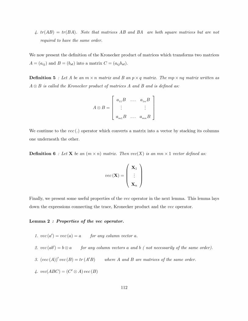
4. tr(AB) = tr(BA). Note that matrices AB and BA are both square matrices but are not
required to have the same order.
We now present the definition of the Kronecker product of matrices which transforms two matrices
A = (aij) and B = (bst) into a matrix C = (aijbst).
Definition 5 : Let A be an m× n matrix and B an p× q matrix. The mp× nq matrix written asA⊗B is called the Kronecker product of matrices A and B and is defined as:
A⊗B =
a11B . . . a1nB...
...
am1B . . . amnB
We continue to the vec (.) operator which converts a matrix into a vector by stacking its columns
one underneath the other.
Definition 6 : Let X be an (m× n) matrix. Then vec(X) is an mn× 1 vector defined as:
vec (X) =
X1...
Xn
Finally, we present some useful properties of the vec operator in the next lemma. This lemma lays
down the expressions connecting the trace, Kronecker product and the vec operator.
Lemma 2 : Properties of the vec operator.
1. vec (a0) = vec (a) = a for any column vector a.
2. vec (ab0) = b⊗ a for any column vectors a and b ( not necessarily of the same order).
3. (vec (A))0 vec (B) = tr (A0B) where A and B are matrices of the same order.
4. vec(ABC) = (C 0 ⊗A) vec (B)
112

5. vec(AB) = (B0 ⊗ Im) vec (A)
= (B0 ⊗A) vec (Im) = (Iq ⊗A) vec (B)
where A is an (m× n) matrix and B is an (n× q) matrix.
The next set of lemmas state some useful properties of the matrix variate t distribution.
Lemma 3 : [Gupta and Nagar (1999), Theorem 4.3.1, pg.135]
Let Z ∼ ZT,m(ν,M,V,Ω), then
E (Z) =M and Cov (vec (Z0)) = 1(ν−2)V⊗Ω, ν > 2.
The above lemma defines the mean and variance-covariance matrix for the matrix variate t
distribution. Our next lemma shows how to use rows and column partitions for deriving the form
of the marginal and conditional distributions starting from the matrix variate t distribution. This
technique is relevant for the derivation of the Student’s t VAR model.
Lemma 4 : [Gupta and Nagar (1999), Theorem 4.3.9]
Let Z ∼ ZT,m(ν,M,V,Ω).
1. Partition Z as follows: Z =
Z1r
Z2r
, where Z1r is a (T1 ×m) matrix and Z2r is a (T2 ×m)and T1 + T2 = T.
2. M can be partitioned in the same way as Z. So M =
M1r
M2r
, where M1r and M2r have
the same dimensions as Z1r and Z2r respectively.
3. V is partitioned as follows: V =
V11 V12
V21 V22
, where V11 is (T1 × T1), V12 is (T1 × T2) ,V21 is (T2 × T1) and V22 is (T2 × T2) .
4. Finally, Ω need not be partitioned since we are partitioning in terms of rows.
113

Then,
(a) the functional form of marginal distribution of this row partition denoted by Z2r ∼ZT2(ν,M2r,V22,Ω) can be represented as follows:
f1(Z2r) =ΓT2
£12 (ν +m+ T2 − 1)
¤π12mT2ΓT2
£12 (ν + T2 − 1)
¤ det (V22)− 12m det (Ω)−
12T2
det¡Im +Ω
−1 (Z2r −M2r)0V−122 (Z2r −M2r)
0¢− 12(ν+m+T2−1)
(b)Similarly, the conditional distribution is denoted as
Z1r|Z2r ∼ ZT1,m ν + T2, M1r +V12V
−122 (Z2r −M2r),
V11.2,Ω(Im +Ω−1(Z2r −M2r)
0V−122 (Z2r −M2r))
where V11.2 = V11 −V12V−122 V21, and the conditional distribution’s functional form is given
by:
f(Z1r|Z2r) = ΓT1 [12(ν+m+T−1)]
π12mT1ΓT1 [
12(ν+T2−1)]
det¡Im +Ω
−1 (Z2r −M2r)0V−122 (Z2r −M2r)
0¢− 12T
det (Ω)−12T1 det((V11.2)
−12m) det(Im + (Im +Ω
−1(Z2r −M2r)0V−122 (Z2r −M2r))
−1
Ω−1(Z1r −M1r −V12V−122 (Z2r −M2r))0
V−111.2(Z1r −M1r −V12V−122 (Z2r −M2r)))− 12(ν+m+T−1)
(6.3)
Remark 2: Row partitions (of the type shown above) can be used to model the temporal in-
terdependencies between the variables. Recall that Ω represents the contemporaneous variance
covariance matrix and therefore need not be partitioned. Note that since we condition on Z2r the
degree of freedom parameter now becomes ν+T2. Column partitions can be done in a similar way.
Using the above lemma on row partitions we can express the matrix variate t distribution
as a product of multivariate densities. By letting T1 = 1, T2 = T − 1, Z1r = Z1 and Z2r =
(Z2,Z3, . . .ZT ), as before the conditional density of this row partition becomes:
114

Z1|Z2r ∼ Z1,m ν + T − 1, M1r +V12V
−122 (Z2r −M2r),
Ω(Im +Ω−1(Z2r −M2r)V
−122 (Z2r −M2r)
0),V11.2
Observe that we can repeat this procedure (T − 1) times sequentially for all variables Zi, i =2, . . . , T − 1. Then we can decompose the density of Z as a product of (T − 1) conditionaldistributions and one marginal distribution as shown below:
f (Z) = f1 (Z1|Z2,Z3, . . .ZT ) f2 (Z2|Z3, . . .ZT ) ...f2 (ZT−1|ZT ) fT (ZT )
where every density on the right hand side is an m dimensional multivariate t density. Information
in the matrix t distribution can thus be expressed by the product of T (m− dimensional) Studentt densities. This decomposition will be crucial in the derivation of the Student’s t VAR model.
Next we present some useful results of Toeplitz matrices and their inverses.
6.2.2 Some Important Results on Toeplitz Matrices
Toeplitz matrices appear in a wide variety of applications including structural engineering, econo-
metrics, seismology, etc. The structure of these matrices3 allows for a reduction in the number of
parameters and is thus useful in estimation and testing. In econometrics we encounter Toeplitz
matrices in time series analysis of stationary stochastic processes and in particular, the variance-
covariance matrices of such processes usually have a Toeplitz structure. We start with the definition
of a Toeplitz matrix.
Definition 7 : A matrix VT (T × T ) is called real Toeplitz matrix if its elements obey the rulevij = vi−j for all i, j = 1, . . . , T, and vij ∈ R. The matrix VT has the following structure:
3For an exhaustive survey of the properties of Toeplitz matrices see Mukherjee and Maiti (1988), and Pustyl’nikov(1984).
115

VT =
v0 v1 v2 . . . vT−2 vT−1
v−1 v0 v1 . . .
v−2 v−1 v0 . . .
v2 v−1 . . .
. . . . . . . . . . . . . . .
v−T+2 . . . v0 v1
v−T+1 . . . v−1 v0
The Toeplitz matrices we encounter in econometric applications are often symmetric and positive
definite. So next we define a symmetric Toeplitz matrix.
Definition 8 : A matrix VT (T × T ) is called real symmetric Toeplitz matrix if its elements obeythe rule vij = v|i−j| for all i, j = 1, . . . T. The matrix VT is a function of T parameters i.e.,
VT = VT (v0, v1, . . . vT−1) and is centrosymmetric4. It has the following structure:
VT =
v0 v1 v2 . . . vT−2 vT−1
v1 v0 v1 . . .
v2 v1 v0 . . .
v2 v1 . . .
. . . . . . . . . . . . . . .
vT−2 . . . v0 v1
vT−1 . . . v1 v0
Another important issue that received a lot of attention in the literature is the problem of in-
version of matrices with Toeplitz structure. This is of particular interest to econometricians, since
Toeplitz matrices with banded inverses arise in studying variance-covariance matrices of autore-
gressive and moving average processes (see Barrett (1984)). Hence, we now present the definition
of a p-banded matrix.
Definition 9 : A matrix Q is p-banded if qij = 0 for |i− j| > p. For p = 2, the matrix Q can bewritten as follows:
4A T × T matrix V is centrosymmetric if vij = vT+1−i,T+1−j for all i, j = 1, . . . , T .
116

Q =
q0 q1 . . . 0
q1 q0 q1 . . . 0
q1 q0 . . . 0
. . . . . . . . . . . . . . .
0 0 0 . . . q1
0 0 0 q1 q0
The next lemma states the conditions that make the inverse of a Toeplitz matrix a p-banded
matrix.
Lemma 5 : [Proposition 1 Spanos (1990), pg. 12]
Let VT = [vi−j ]T−1i,j=0 be a non-singular, symmetric Toeplitz matrix, i.e.
VT =
v0 v1 v2 . . . vT−2 vT−1
v1 v0 v1 . . .
v2 v1 v0 . . .
v2 v1 . . .
. . . . . . . . . . . . . . .
vT−2 . . . v0 v1
vT−1 . . . v1 v0
such that |vk| ≤ cλk, 0 < c <∞, 0 < λ < 1, k = 1, 2, . . .
Then QT = V−1T :
(a) is a p-banded matrix i.e., qij = 0 for |i− j| > p.
(b) qij = qkm for |i− j| = |k −m| > 0 for ordered pairs (i, j) 6= (k,m) .
Hence for p = 2,
117

QT =
q11 q12 q2 0 0 . . . 0 0
q12 q22 q1 q2 0 . . . 0 0
q2 q1 q0 q1 q2 . . . 0 0
0 q2 q1 q0 q1 . . . 0 0
. . . . . . . . . . . . . . . . . . . . . . . .
0 0 0 0 0 . . . q1 q2
0 0 0 0 0 . . . q22 q12
0 0 0 0 0 . . . q12 q11
Note that qij = 0 for |i− j| > p and qij is a function of |i− j| for |i− j| < p, except in the
p× p submatrix in the upper left and lower right corners of QT . These two submatrices are mirrorimages of each other and contain terms that are different from the rest of the matrix. Moreover
each of these matrices is symmetric along its main diagonal. In fact, QT is a quasi -Toeplitz and
persymmetric5 matrix. For p = 2, the number of distinct elements in QT is 6 and when p = 3 it is
10. In general note that the number of distinct elements in the QT matrix is(p+1)(p+2)
2 .
6.2.3 Matrix Calculus and Differentials
The purpose of this sub-section is to introduce the notion of the differential for obtaining partial
derivatives that involve matrix, vector and scalar functions of scalar, vector and matrix variables.
It is has been argued that this approach based on the differential (which is different from the
traditional matrix derivatives approach) is ideally suited for the type of multivariate functions that
we encounter in econometrics6. We begin by defining the differential and then presenting the First
Identification Theorem which is the corner stone of the differential approach since it is used to
obtain the derivative (the Jacobian matrix) from the differential.
Definition 10 Let f : S → Rm be a function defined on a set S in Rn. Let c be an interior
point of S, and let B(c; r) be an n−ball lying in S. Let u be a point in Rn with kuk < r, so that
5A (T × T ) matrix V is persymmetric if it is symmetric with respect to the diagonal from the upper right handcorner to the lower left hand corner. A quasi-Toepltz matrix is a matrix that has a Toeplitz like structure.
6For more on the advantages of this approach and how it differs from the traditional one see the introductorychapters in Magnus and Neudecker (1999).
118

c + u ∈ B(c; r). If there exists a real m × n matrix A, depending on c but not on u, such thatf(c+ u) = f(c) +Ac(u) + rc(u) for all u in Rn with kuk < r, and
limu→0
rc(u)
kuk = 0, (6.4)
then the function f is said to be differentiable at c and rc(u) is the remainder term in the first
order Taylor’s expansion, which is of smaller order than u as u −→ 0. The m× n matrix A(c) isthen called the (first) derivative of f at c, and the m× 1 vector df(c;u) = A(c)u, which is a linearfunction of u is called the (first) differential of f at c (with increment u).
We now state the primary result used in the differential approach.
Lemma 6 : [First Identification Theorem, Magnus and Neudecker, (1999) pg. 87]
(a) For vector function: Let f : S → Rm be a vector function defined on a set S in Rm, and
differentiable at an interior point c of S. Let u be a real n× 1 vector. Then
df (c;u) = (Df (c))u,
where df (c;u) represents the differential at c and Df (c) is an m × n matrix whose elementsDjfi (c)are the partial derivatives of f evaluated at c.
(b) For matrix functions: Let F : S → Rm×p be a matrix function defined on a set S in Rn×q,
and differentiable at an interior point C of S. Then
vecdF (C;U) = A (C) vecU,
for all U ∈ Rn×q if and only if DF (C) = A (C).
This theorem has great practical value since computations with differentials are relatively easy
and once we have found the differential the value of the partial derivatives can be immediately
determined. Another result that we use throughout is the extension of the chain rule for matrix
functions. This is stated in the next lemma.
119
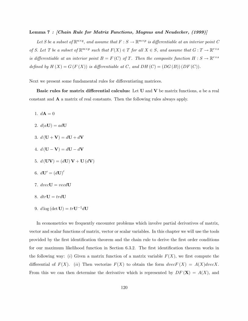
Lemma 7 : [Chain Rule for Matrix Functions, Magnus and Neudecker, (1999)]
Let S be a subset of Rn×q, and assume that F : S → Rm×p is differentiable at an interior point C
of S. Let T be a subset of Rm×p such that F (X) ∈ T for all X ∈ S, and assume that G : T → Rr×s
is differentiable at an interior point B = F (C) of T . Then the composite function H : S → Rr×s
defined by H (X) = G (F (X)) is differentiable at C, and DH (C) = (DG (B)) (DF (C)).
Next we present some fundamental rules for differentiating matrices.
Basic rules for matrix differential calculus: Let U and V be matrix functions, a be a real
constant and A a matrix of real constants. Then the following rules always apply.
1. dA = 0
2. d(aU) = adU
3. d (U+V) = dU+ dV
4. d (U−V) = dU− dV
5. d (UV) = (dU)V +U (dV)
6. dU0 = (dU)0
7. dvecU = vecdU
8. dtrU = trdU
9. d log (detU) = trU−1dU
In econometrics we frequently encounter problems which involve partial derivatives of matrix,
vector and scalar functions of matrix, vector or scalar variables. In this chapter we will use the tools
provided by the first identification theorem and the chain rule to derive the first order conditions
for our maximum likelihood function in Section 6.3.2. The first identification theorem works in
the following way: (i) Given a matrix function of a matrix variable F (X), we first compute the
differential of F (X). (ii) Then vectorize F (X) to obtain the form dvecF (X) = A(X)dvecX.
From this we can then determine the derivative which is represented by DF (X) = A(X), and
120
A(X) contains the partial derivatives. The maximum likelihood function is a scalar function of
potentially scalar, vector and matrix variables. Consequently, to obtain the partial derivatives
from DF (X) we use the result stated below:
Dφ (X) =
µvec
µ∂φ (X)
∂ (X)
¶¶0(6.5)
where φ (.) represents a scalar function and X is a matrix variable.
6.3 Student’s t VAR Model
In this section we specify the Student’s t Vector Autoregressive Model using the Probabilistic
Reduction approach. The VAR representation enables us to model the dynamic interdependence
between the variables in Zt, since every variable depends linearly on the history of all the other
variables. This is particularly important in Financial Econometrics, since it provides a realistic and
sensible model that can capture the dynamic interrelationship between the volatilities of the differ-
ent variables. Moreover, the choice of Student’s t distribution implies a particular functional form
for the conditional variance which enables us to model the empirical regularities of leptokurticity,
non-linear dependence, heteroskedasticity and variance heterogeneity that is observed in speculative
price data.
6.3.1 Specification
In the context of the Probabilistic Reduction approach, the VAR can be viewed as the statistical7
model, that provides a summary of the systematic information in the observed multivariate process
Zt, t ∈ T. The operational VAR model is specified by imposing certain reduction assumptions
on the joint distribution of the vector stochastic process Zt, t ∈ T. The reduction assumptionsare derived from the probabilistic features of the underlying stochastic process and can be sum-
marized into three categories: Distributional assumption, Dependence and (time) Heterogeneity
assumptions. For the Student’ t VAR model the reduction assumptions are given by:
7Note that in the context of the PR approach the statistical model need not coincide with the economic theorymodel under investigation.
121

1. Distribution: Matrix variate t
Let Z be a (T ×m) matrix of m variables over T time periods. The joint distribution of
the underlying vector stochastic process Zt, t ∈ T is a matrix variate t distribution. UsingLemma 3 from Section 6.2 it can be expressed as follows:
vec(Z0) =
Z1
Z2
.
.
.
ZT
∼ StT,m
µ(1)
µ(2)
.
.
.
µ(T )
,
v11Ω v12Ω v13Ω . v1TΩ
v21Ω v22Ω v23Ω . v2TΩ
v31Ω v31Ω v33Ω . .
. . .
. . .
. .
vT1Ω vT2Ω vTTΩ
; ν
(6.6)
where Zt = (Zt1,Zt2, . . . Ztm)0 , and µ(t) =
¡µ1,µ2, . . . µm
¢0are (m × 1) vectors, V is a (T × T )
temporal covariance matrix, Ω is an (m×m) contemporaneous variance-covariance matrix andCov(vec(Z0)) = 1
ν−2 (V⊗Ω) is a (Tm× Tm) matrix.
2. Dependence: Markov(p)
We assume a Markov process of order p so as to allow for any weak form of linear dependence
that might be present in the data. This means that the conditional mean of Zt can be
described by a Markov (p) process.
3. Heterogeneity: Second Order Stationarity
This conditions allows us to express the first two moments. We can write the mean as:
E (Zt) = µ(t) = µ for all t ∈ T.
122
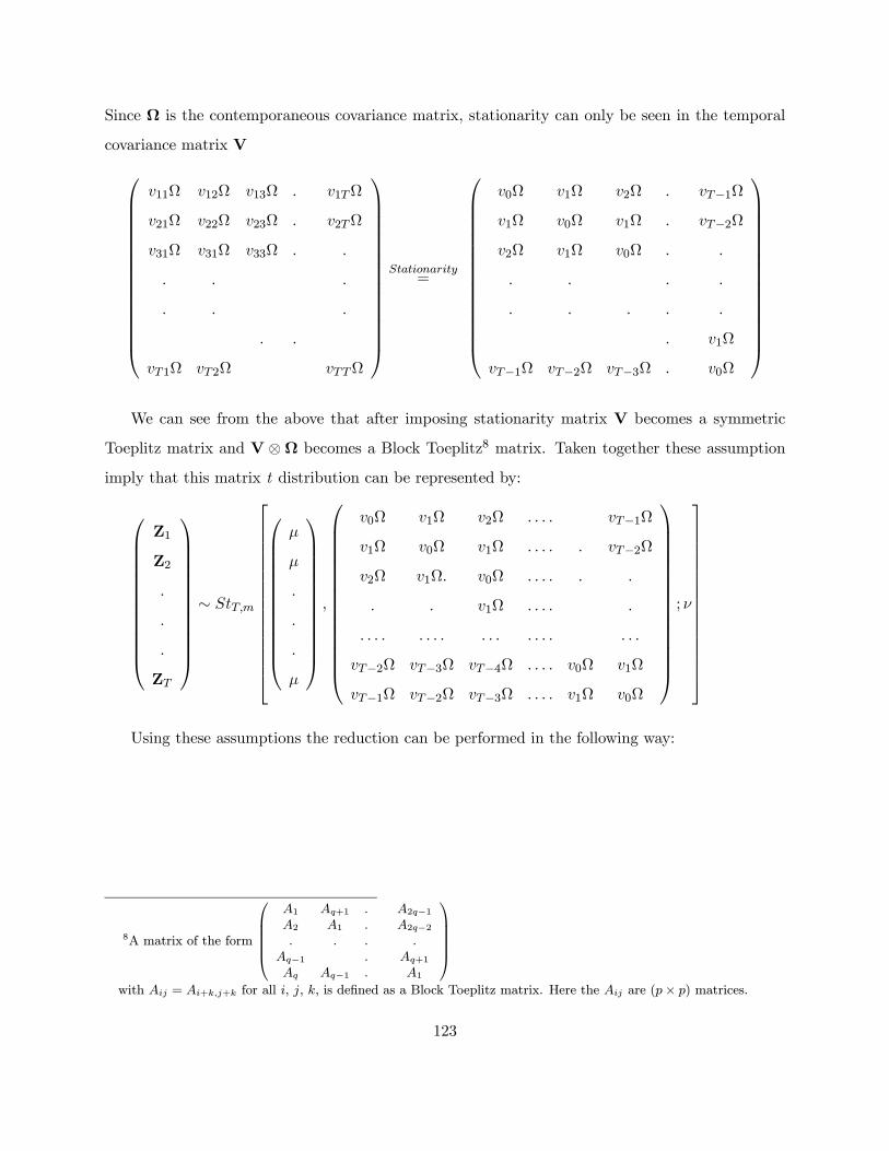
Since Ω is the contemporaneous covariance matrix, stationarity can only be seen in the temporal
covariance matrix V
v11Ω v12Ω v13Ω . v1TΩ
v21Ω v22Ω v23Ω . v2TΩ
v31Ω v31Ω v33Ω . .
. . .
. . .
. .
vT1Ω vT2Ω vTTΩ
Stationarity=
v0Ω v1Ω v2Ω . vT−1Ω
v1Ω v0Ω v1Ω . vT−2Ω
v2Ω v1Ω v0Ω . .
. . . .
. . . . .
. v1Ω
vT−1Ω vT−2Ω vT−3Ω . v0Ω
We can see from the above that after imposing stationarity matrix V becomes a symmetric
Toeplitz matrix and V ⊗Ω becomes a Block Toeplitz8 matrix. Taken together these assumptionimply that this matrix t distribution can be represented by:
Z1
Z2
.
.
.
ZT
∼ StT,m
µ
µ
.
.
.
µ
,
v0Ω v1Ω v2Ω . . . . vT−1Ω
v1Ω v0Ω v1Ω . . . . . vT−2Ω
v2Ω v1Ω. v0Ω . . . . . .
. . v1Ω . . . . .
. . . . . . . . . . . . . . . . . .
vT−2Ω vT−3Ω vT−4Ω . . . . v0Ω v1Ω
vT−1Ω vT−2Ω vT−3Ω . . . . v1Ω v0Ω
; ν
Using these assumptions the reduction can be performed in the following way:
8A matrix of the form
A1 Aq+1 . A2q−1A2 A1 . A2q−2. . . .
Aq−1 . Aq+1Aq Aq−1 . A1
with Aij = Ai+k,j+k for all i, j, k, is defined as a Block Toeplitz matrix. Here the Aij are (p× p) matrices.
123
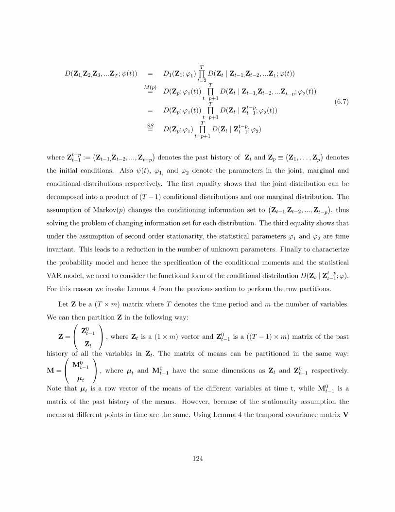
D(Z1,Z2,Z3, ...ZT ;ψ(t)) = D1(Z1;ϕ1)TQt=2D(Zt | Zt−1,Zt−2, ...Z1;ϕ(t))
M(p)= D(Zp;ϕ1(t))
TQt=p+1
D(Zt | Zt−1,Zt−2, ...Zt−p;ϕ2(t))
= D(Zp;ϕ1(t))TQ
t=p+1D(Zt | Zt−pt−1;ϕ2(t))
SS= D(Zp;ϕ1)
TQt=p+1
D(Zt | Zt−pt−1;ϕ2)
(6.7)
where Zt−pt−1 :=¡Zt−1,Zt−2, ...,Zt−p
¢denotes the past history of Zt and Zp ≡
¡Z1, . . . ,Zp
¢denotes
the initial conditions. Also ψ(t), ϕ1, and ϕ2 denote the parameters in the joint, marginal and
conditional distributions respectively. The first equality shows that the joint distribution can be
decomposed into a product of (T −1) conditional distributions and one marginal distribution. Theassumption of Markov(p) changes the conditioning information set to
¡Zt−1,Zt−2, ...,Zt−p
¢, thus
solving the problem of changing information set for each distribution. The third equality shows that
under the assumption of second order stationarity, the statistical parameters ϕ1 and ϕ2 are time
invariant. This leads to a reduction in the number of unknown parameters. Finally to characterize
the probability model and hence the specification of the conditional moments and the statistical
VAR model, we need to consider the functional form of the conditional distribution D(Zt | Zt−pt−1;ϕ).
For this reason we invoke Lemma 4 from the previous section to perform the row partitions.
Let Z be a (T ×m) matrix where T denotes the time period and m the number of variables.
We can then partition Z in the following way:
Z =
Z0t−1Zt
, where Zt is a (1×m) vector and Z0t−1 is a ((T − 1)×m) matrix of the pasthistory of all the variables in Zt. The matrix of means can be partitioned in the same way:
M =
M0t−1µt
, where µt and M0t−1 have the same dimensions as Zt and Z0t−1 respectively.
Note that µt is a row vector of the means of the different variables at time t, while M0t−1 is a
matrix of the past history of the means. However, because of the stationarity assumption the
means at different points in time are the same. Using Lemma 4 the temporal covariance matrix V
124

is partitioned as follows:
V =
V11 V12
V21 V22
=
v0 v1 v2 . . . vT−2
v1 v0 v1 . . .
v2 v1 v0 . . .
v2 v1 . . .
. . . . . . . . . . . .
vT−2 . . . v0
vT−1
. . .
v1
³vT−1 . . . v1
´[v0]
Observe that V11 is a ((T − 1)× (T − 1)) symmetric Toeplitz matrix, V12 is a ((T − 1) × 1)
column vector, V21 is the transpose of V12, and V22 is now a scalar denoted by v0. Consequently
V22.1 is now a scalar since:
V22.1 = V22 −V21 (V11)−1V12
= v0 −³vT−1 . . . v1
´
v0 v1 v2 . . . vT−2
v1 v0 v1 . . .
v2 v1 v0 . . .
v2 v1 . . .
. . . . . . . . . . . .
vT−2 . . . v0
−1
vT−1
. . .
v1
We denote V22.1 by σ
2. Also from Lemma 5 the inverse of V11 is a p-banded matrix denoted by
Q0t−1. Finally Ω, that is the contemporaneous variance-covariance matrix need not be partitioned
since we are partitioning in terms of rows (which in this case is time).
The functional form of the conditional distribution assuming p lags9 can thus be expressed as:
9By assuming Markov of order p, we need to consider only the past history up to p periods.
125

f(Zt|Z0t−1) =Γ[ 12 (ν+m+T−1)]π12mΓ[ 12 (ν+T−1)]
det
µIm +Ω
−1³Zt−pt−1 −Mt−p
t−1´0Qt−pt−1
³Zt−pt−1 −Mt−p
t−1´¶− 1
2
det (Ω)−12
det³σ2)−
12m´det[(Im + (Im +Ω
−1(Zt−pt−1 −Mt−pt−1)
0Qt−pt−1(Zt−pt−1 −Mt−p
t−1))−1
Ω−1(Zt −µt −V21Qt−pt−1(Zt−pt−1 −Mt−p
t−1))0¡
σ2¢−1
(Zt −µt −V21Qt−pt−1(Zt−pt−1 −Mt−p
t−1))]−12(ν+m+T−1)
(6.8)
where m is the number of variables in Zt. Notice that this is similar to the conditional distribution
that we had in Lemma 4. In order to re-write the above in a simpler way. Both Ct and Dt arem×m matrices and can be defined as follows:
Ct =
·(Im +Ω
−1³Zt−pt−1 −Mt−p
t−1´0Qt−pt−1
³Zt−pt−1 −Mt−p
t−1´¸
and
Dt =
µCt +
·1
σ2Ω−1U 0tUt
¸
We define Ut which is an 1×m vector as follows:
Ut =£Zt − µ(Im −B11mp,m)− (B1Z0t−1)0
¤which is an 1×m vector. Note that Ω−1, is an m×m, symmetric and p.d. matrix,
³Qt−pt−1
´, is a
p× p symmetric and p.d. matrix, and σ2, is a positive scalar. Finally note that B1, is an m×mpmatrix of coefficients µ, is an 1×m vector of means, 1mp,m, is a an mp×m matrix of ones, 11×p,
is a 1× p vector of ones, Zpt−1, is an p×m matrix of data and zpt−1, is an mp× 1 vector of data.
This allows us to rewrite equation 6.8 as:
f(Zt|Z0t−1) =Γ[ 12 (ν+m+T−1)]π12mΓ[ 12 (ν+T−1)]
det (Ct)−12 det (Ω)−
12
det³¡σ2¢− 1
2m´det(Ct + 1
σ2Ω−1U 0tUt)−
12(ν+m+T−1)
(6.9)
126

The following proposition enables us to specify the Student’s t VAR model based on the first
two moments of f(Zt|Z0t−1).
Proposition 1 Let Zt, t ∈ T be a Student’s t with ν (ν > 1) degrees of freedom, stationary
stochastic process with stable vector autoregressive representation, then the first two moments of
f(Zt|Z0t−1) take the following form:
The conditional mean can be expressed as:
E(Zt|σ(Zt−1) = B0 +pPi=1BiZt−i +Ut, t ∈ N (6.10)
where p is the number of lags in the conditional mean because of the Markov(p) assumption. The
conditional variance-covariance matrix can be written as:
Cov(Zt|σ(Zt−1)) =h
νν+mp−2
iΩ(Im +Ω
−1 pPi=1
pPj=1
qij(Zt−i − µ)0(Zt−j − µ) (6.11)
where qij = 0 for |i− j| > p, qij = qkl for |i− j| = |k − l|
Proof. The result follows from lemma 4:
E(ZtÁσ(Zt−1) =M1r +V12V−122 (Z2r −M2r)
= µt −V21Q0t−1(Z0t−1 −M0t−1)
= µ(Im −B11mp,m)− (B1Z0t−1)0
Cov(ZtÁσ(Zt−1)) = Ω(Im +Ω−1(Z2r −M2r)V−122 (Z2r −M2r)
0)
= Ω
µIm +Ω
−1³Zt−pt−1 −Mt−p
t−1´0Qt−pt−1
³Zt−pt−1 −Mt−p
t−1´
From lemma (5)³Q (i, j) |t−1i,j=1
´≡³V (|i− j|) |t−1i,j=1
´is p−banded and ‘quasi-Toeplitz’, giving
rise to:
127

Student’s t Vector Autoregressive Model
E(Zt|σ(Zt−1) = B0 +pPi=1BiZt−i +Ut, t ∈ N (6.12)
Cov(Zt|σ(Zt−1)) =h
νν+mp−2
iΩ(Im +Ω
−1 pPi=1
pPj=1
qij(Zt−i − µ)0(Zt−j − µ) (6.13)
where qij = 0 for |i− j| > p, qij = qkl for |i− j| = |k − l| .
The conditional mean is a linear function of the conditioning variables like the Normal VAR(1)
process. The conditional variance however, is heteroskedastic and thus can capture the observed
second order dependence. Moreover, we do not need to worry about positive definiteness of the
conditional variance and coefficient restrictions. The conditional variance is a quadratic function of
the past conditioning information, ensuring positive definiteness. Also, overparametrization does
not seem to be a problem any more since there are only p unknown qijs and m(m+1)/2 parameters
in Ω. The conditional mean and the conditional variance parametrizations are interrelated. In
particular the parameters (the B matrix and the and qij) are both defined in terms of the (QT )
matrix.
Example 1 : For the purpose of exposition we will now show the VAR(1) case. In this case the
reduction takes the form:
D(Z1,...,ZT ;ψ(t)) = D1(Z1;ϕ1)TQt=2D(Zt | Zt−1,Zt−2, ...Z1;ϕ2(t))
M(1)= D(Z1;ϕ1(t))
TQt=2D(Zt | Zt−1;ϕ2(t))
SS= D(Z1;ϕ1)
TQt=2D(Zt | Zt−1;ϕ2) (Z1,Z2,Z3, ...ZT ) ∈ RmT
(6.14)
The specific expressions for D(Zt | Zt−1;ϕ) can be obtained using the results of the previoussection. The Student’s t VAR(1) model can be fully specified as shown in Table 6.1. It is interesting
128

The Student’s t VAR(1) Model
I. Statistical GM: Zt = B0 +B1Zt−1 +Ut, t ∈ T.
[1]Dt = Z0t−1 is the relevant conditioning information set withµt = E(Zt | Z0t−1) = B0 +B1Zt−1 : the systematic component, andUt = Zt −E(Zt | Zt−1) : the non-systematic component.[2]ϕ := (B0,B1,Ω,V11), are the statistical parameters of interest, where
B0 = E (Zt)−B1E(Zt−1), B1 = [cov(Zt−1)]−1 cov¡Zt,Zt−1
¢.
[3]The roots of det [Imλ−B1, ] = 0 have modulus less than one.[4]No a priori restrictions on ϕ := (B0,B1,V11,Ω,).[5]Rank(Z1,...,ZT ) = m.
II. Probability model: Φ = D(Zt | Zt−1;ϕ), ϕ := (B0,B1,V11,Ω), Zt ∈ Rm .
[6]
(i) D(Zt | Zt−1;ϕ) is Student’s t,(ii) E(Zt | Zt−1;ϕ) = B0 +B1Zt−1 is linear in Zt−1,(iii) Cov(Zt | Zt−1) =
hν
ν+m−2iΩ(Im +Ω
−1(Zt−1 − µ)0V−111 (Zt−1 − µ)) is heteroskedastic.[7]The parameters ϕ := (B0,,B1,V11,Ω,) are t-invariant.
III. Sampling model:[8](Z1,Z2,...,ZT ) is a Markov/stationary sample drawn from D(Zt | Z0t−1;ϕ) t ∈ T.
Table 6.1: The PR Approach: Student’s t VAR(1) Specification
to see how the reduction assumptions relate to the probabilistic assumptions of the Student’s t VAR
model. This is shown is Table 6.2.
129

Reduction Assumptions: Model Assumptions:Zt, t ∈ T (Zt | Zt−1;ϕ), t ∈ T
Student’s t −→
(i) D(Zt | Zt−1;ϕ) is Student’s t(ii) E(Zt | Zt−1) = B0 +B1Zt−1 is linear in Zt−1
(iii)
Cov(Zt | Zt−1) =hν
ν+m−2iΩ(Im +Ω
−1(Zt−1 − µ)0V−111 (Zt−1 − µ))is heteroskedastic,
Markov −→ (Ut | Zt−1) , t ∈ T is a martingale difference process
Stationarity −→ The parameters (B0,B1,V11,Ω) are t-invariant.
Table 6.2: Reduction and Probability Model Assumptions: Student’s t VAR
6.3.2 Maximum Likelihood Estimation
The likelihood function is based on the sequential decomposition of the joint distributionD(Z1,Z2,Z3,
...ZT ;ψ(t)) as defined by the Probabilistic Reduction assumptions mentioned earlier. After impos-
ing the assumptions of Markov(p) and Stationarity, and assuming that the past information can be
summarized by the last observations this reduction takes the form:
D(Z1,Z2,Z3, ...ZT ;ψ(t)) = D(Zp;ϕ1)TQ
t=p+1D(Zt | Zt−pt−1;ϕ2)
where Zt−pt−1 :=¡Zt−1,Zt−2, ...,Zt−p
¢denotes the past history of Zt and Zp ≡ (Z1, . . . , Zp) denotes
the initial conditions. The log likelihood takes its usual form
lnL (θ;Z1,Z2,Z3, ...ZT ) ∝ D(Zp;ϕ1)TQ
t=p+1D(Zt | Zt−pt−1;ϕ2)
This allows us to write the likelihood function as shown on the next page:
130

The Loglikelihood Function:
lnL (θ;Z1,Z2,Z3, ...ZT ) = (T − 1) lnΓ £12 (ν +m+ T − 1)¤− 12m(T − 1) ln (π)
− (T − 1)Γ £12 (ν + T − 1)¤+ 12(T − 1) ln(det
¡Ω−1
¢)
−12m(T − 1) ln(detσ2)− 12
TPt=2ln det(Ct)− 1
2
TPt=2ln det(Dt)
(6.15)
The first three terms can be treated as a constant and the log-likelihood can be rewritten as:
lnL (θ;Z1,Z2,Z3, ...ZT ) = constant +12(T − 1) ln(det
¡Ω−1
¢)
−12m(T − 1) ln(det¡σ2¢) −12
TPt=2ln det(Ct)− 1
2
TPt=2ln det(Dt)
Recall that Ω−1 is an m×m symmetric and p.d matrix, and³Qt−pt−1
´is a p× p symmetric and p.d
matrix, while σ2 is a positive scalar. Both Dt and Ct are m×m matrices that have been defined
as follows:
Ct =
·(Im +Ω
−1³Zt−pt−1 − µ. ∗ 11×p
´³Qt−pt−1
´³Zt−pt−1 − µ. ∗ 11×p
´0¸and
Dt =
µCt +
·1
σ2Ω−1UtU
0t
¸
we define Ut which is an m× 1 vector as follows:
Ut =£Zt − (Im −B11mp,m)µ−B1Zt−pt−1
¤Finally note that B1 is an m×mp matrix of coefficients, µ is an m× 1 vector of means, 1mp,m isa an mp×m matrix of ones, 11×p is a 1× p vector of ones, Zt−pt−1 is an m× p matrix of data, andzt−pt−1 is an mp× 1 vector of data.
To estimate the unknown parameters, this likelihood needs to be maximized with respect to
B1, Ω−1, Q0t−1, µ and σ2, i.e., we need the partial derivatives shown below.
∂Lnl∂B1
∂Lnl∂Ω−1
∂Lnl∂(Q0
t−1)∂Lnl∂µ
∂Lnl∂σ2
131

Proposition 2 : The first order conditions for the log likelihood function are as follows:
∂Lnl
∂σ2= −1
2m(T − 1) 1
σ2+1
2
TXt=2
trD−1t1
σ4Ω−1UtU 0t = 0 (6.16)
∂Lnl
∂¡Q0t−1
¢ = −12
TXt=2
(A0t−1Ω0−1 ¡C0−1t ¢
At−1)− 12
TXt=2
(A0t−1Ω0−1 ¡D0−1
t
¢At−1) = 0 (6.17)
∂Lnl
∂ (Ω−1)=
12(T − 1) (Ω)− 1
2
TPt=2(I0mC
0−1t (At−1
¡Q0t−1
¢A0t−1)
−12TPt=2(I0mD
0−1t (At−1
¡Q0t−1
¢A0t−1) + (I0mD
0−1t (UtU
0t)0)
= 0 (6.18)
∂Lnl
∂ (B1)=
−12
TPt=2Im¡U 0t
1σ2Ω−1D0−1
t Im¢ ¡Imk,mµ− Z0t−1
¢0−12
TPt=2I
Im¡I0m 1
σ2Ω−1D0−1
t ImUt¢ ¡Imk,mµ− Z0t−1
¢0 = 0 (6.19)
∂Lnl
∂ (µ)=
12
TPt=2
hI0m¡Q0t−1A0t−1C
−1t Ω
−1¢0 101×ki+ ·I0m ³Q00t−1A0t−1 (Ω0)−1 (C0t)−1´0 101×k¸−12
TPt=2−µhI0m¡Q0t−1A0t−1D
−1t Ω
−1¢0 101×ki+ ·I0m ³Q00t−1A0t−1 (Ω0)−1 (D0t)−1´0 101×k¸
−12TPt=2
¡U 0tD
−1t
1σ2Ω−1(B11mk,m − Im)
¢0+³U 0tΩ−1 1σ2 (D
0t)−1 (B11mk,m − Im)
´0
= 0
(6.20)
Proof. Here we show the proofs for ∂Lnl∂σ2
and ∂Lnl∂(Q0
t−1). The rest are shown in the Appendix.
(a) Partial derivative for σ2 : We need to consider only the relevant terms in the likelihood
function. Following Magnus and Neudecker (1999) we are concerned only with the differential of
σ2. So, using the fact that d ln det(Dt) = det(Dt)−1ddet(Dt) we obtain
d lnL = −12m(T − 1) 1
σ2− 12
TXt=2
det(Dt)−1ddet(Dt)
Recall that ddet(Dt) = det(Dt)trD−1t dDt. Hence, we get
d ln det(Dt) = det(Dt)−1 det(Dt)trD
−1t dDt
= trD−1t dDt
132

Substituting the fact that Dt =¡Ct +
£1σ2Ω−1UtU 0t
¤¢, we obtain
dDt(σ2) = dCt +
£d(σ2)−1Ω−1UtU 0t
¤= 0− 1
σ4Ω−1UtU 0t
This allows us to write the partial derivative as
∂Lnl
∂σ2= −1
2m(T − 1) 1
σ2+1
2
TXt=2
trD−1t1
σ4Ω−1UtU 0t = 0
(b) Partial Derivative for Q0t−1 : Focusing on the relevant terms in the likelihood function
allows us to write the differential as
d lnL = −12
TXt=2
d ln det(Ct)− 12
TXt=2
d ln det(Dt)
Consider the first term on the right hand side. Using Property 9 of the differentials we can
express this as: d ln det(Ct) = det(Ct)−1 det(Ct)trC−1t dCt = trC−1t dCt. Recall that tr(A0B) =
vec(A)0vec(B) and from Lemma 2 we know that vec(ABC) = (C 0⊗A)vec(B). Applying these twoproperties we have
d ln det(Ct) = trC−1t dCt = vec(C
0−1t )0vec(dCt)
Next defineAt−1 =¡Z0t−1 − µ. ∗ 11×k
¢. This allows us to expressCt as
£(Im +Ω
−1At−1¡Q0t−1
¢A0t−1
¤.
Hence we have vec(dCt(Q0t−1)) = vec(dIm) + vec(Ω
−1At−1¡dQ0t−1
¢A0t−1) which we can write as
vec(dCt(Q0t−1)) = 0 + (At−1 ⊗ Ω−1At−1)vec(dQ0t−1). Using Lemma 2 again and the fact that
[vec(ABC)]0 = [(C 0 ⊗A)vec(B)]0 = vec(B)0(C0 ⊗A)0 = vec(B)0(C ⊗A0), we can obtain
d ln det(Ct) = vec(C0−1t )0vec(dCt)
Note that this can be rewritten as vec(C0−1t )0(At−1 ⊗Ω−1A)dvec(Q0t−1). With some more manip-
133

ulation we now obtain∂Lndet(Ct)
∂¡Q0t−1
¢ = (A0t−1Ω0−1 ¡C0−1t ¢
At−1)
Now we will consider the second term 12
TPt=2d ln det(Dt) in the likelihood function. Note that
Q0t−1 appears inDt only through Ct. Consequently, d ln det(Dt) = trD−1t dDt = vec(D
0−1t )0vec(dDt),
which can be written as vec(D0−1t )0vec(dCt) as the constant terms will vanish from the differen-
tial. Following a similar reasoning outlined above we have ∂Lndet(Dt)
∂(Q0t−1)
= (A0t−1Ω0−1¡D0−1t
¢At−1).
Invoking the first identification theorem, we can now combine the two terms and obtain the partial
derivative of Q0t−1:
∂Lnl
∂¡Q0t−1
¢ = −12
TXt=2
(A0t−1Ω0−1 ¡C0−1t ¢
At−1)− 12
TXt=2
(A0t−1Ω0−1 ¡D0−1
t
¢At−1) = 0.
This completes the proof.
Clearly the first order conditions shown above are non-linear in the parameters and cannot be
solved explicitly. They need to be evaluated iteratively by some numerical algorithm. Moreover,
the second order conditions are analytically intractable.
6.4 Statistical Model Comparisons
In this section we provide a comparison between the parametrizations of the conditional variance
-covariance matrix arising from the Student’s t VAR model and some of the most popular mul-
tivariate GARCH type models. In particular we compare these two types of models in terms of
their properties and specific restrictions (if any). We also compare the Normal VAR model to
the Student’s t VAR simply to bring out the drawbacks of the former for modeling the empirical
regularities in speculative prices. This serves to illustrate how by changing one of the reduction
assumptions, namely the distribution assumption from Normal to Student’s t can lead to a specifi-
cation that can accommodate the probabilistic nature of such data. First we compare the Student’s
t AR specification presented in Chapter 3 to the Student’s t VAR formulation. This is an especially
interesting comparison since both parametrizations are based on the PR approach.
134
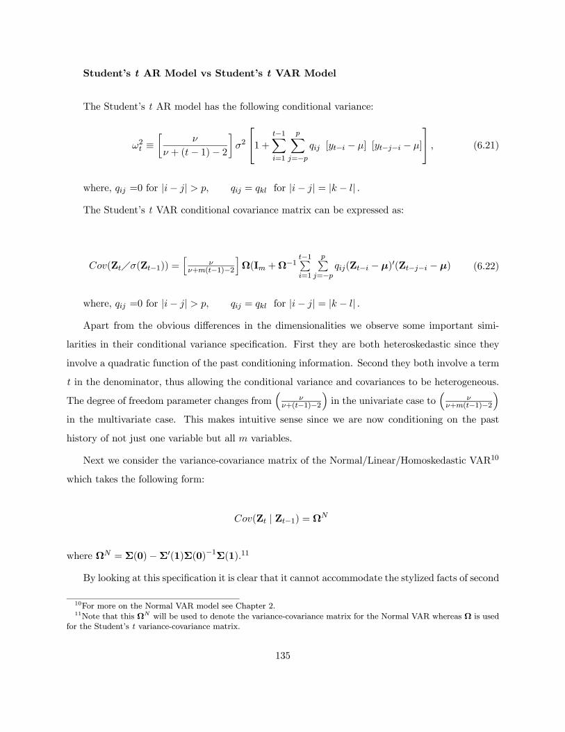
Student’s t AR Model vs Student’s t VAR Model
The Student’s t AR model has the following conditional variance:
ω2t ≡·
ν
ν + (t− 1)− 2¸σ2
1 + t−1Xi=1
pXj=−p
qij [yt−i − µ] [yt−j−i − µ] , (6.21)
where, qij =0 for |i− j| > p, qij = qkl for |i− j| = |k − l| .
The Student’s t VAR conditional covariance matrix can be expressed as:
Cov(ZtÁσ(Zt−1)) =h
νν+m(t−1)−2
iΩ(Im +Ω
−1 t−1Pi=1
pPj=−p
qij(Zt−i −µ)0(Zt−j−i − µ) (6.22)
where, qij =0 for |i− j| > p, qij = qkl for |i− j| = |k − l| .
Apart from the obvious differences in the dimensionalities we observe some important simi-
larities in their conditional variance specification. First they are both heteroskedastic since they
involve a quadratic function of the past conditioning information. Second they both involve a term
t in the denominator, thus allowing the conditional variance and covariances to be heterogeneous.
The degree of freedom parameter changes from³
νν+(t−1)−2
´in the univariate case to
³ν
ν+m(t−1)−2´
in the multivariate case. This makes intuitive sense since we are now conditioning on the past
history of not just one variable but all m variables.
Next we consider the variance-covariance matrix of the Normal/Linear/Homoskedastic VAR10
which takes the following form:
Cov(Zt | Zt−1) = ΩN
where ΩN = Σ(0)−Σ0(1)Σ(0)−1Σ(1).11
By looking at this specification it is clear that it cannot accommodate the stylized facts of second
10For more on the Normal VAR model see Chapter 2.11Note that this ΩN will be used to denote the variance-covariance matrix for the Normal VAR whereas Ω is used
for the Student’s t variance-covariance matrix.
135

order dependence and leptokurticity observed in speculative price data since Normality can only
accommodate first order dependence. The way to overcome this problem from the PR approach is
to postulate an alternative distribution, which embodies these features of the data. The Student’s
t distribution seems to be a natural choice since it is more leptokurtic than the Normal. Moreover,
it gives rise to a conditional variance-covariance specification as shown by equation (6.13), that can
capture higher order dependence by allowing for dynamic heteroskedasticity.
We now provide theoretical comparisons with the multivariate GARCH type parametrizations.
We start with the Vech model. Recall that the general form of the conditional covariance matrix
of an m-dimensional Normal GARCH(p, q) model can be written as:
V ech(Ht) = vech(Σ) +
qXi=1
Aivech(εt−iε0t−i) +
pXj=1
Bjvech(Ht−j)
The number of parameters in the Vector GARCH is: (m (m+ 1) /2) [1 + (p+ q) (m (m+ 1) /2)]
= O¡m4¢. On the other hand the number of parameters in the Student’s t VAR covariance matrix is
(m (m+ 1) /2)+p+1, which is considerably lower. To make the multivariate GARCH formulations
operational a number of different restrictions are imposed on the parameters which gives rise to
a variety of formulations for the conditional variance-covariance matrix. This, in turn raises the
question of ensuring positive definiteness. The Student’s t VAR model however overcomes both of
these problems. Positive definiteness is ensured by definition, and parsimony is ensured by jointly
modeling the conditional mean and variance parameters since they are interrelated through the
Q0t−1 matrix.
The diagonal formulation shown below is one example of imposing unrealistic coefficient re-
strictions. By setting p = q = 1 and imposing diagonality on Ai and Bj , every element of Ht can
be written as:
hijt = σij + aijεi(t−1)εj(t−1) + bijhij(t−1) i, j = 1, 2, . . . N
giving us the diagonal specification. Though the total number of parameters reduces to (p+ q + 1)
(m (m+ 1)Á2) = O¡m2¢, there is also a corresponding loss in terms of interpretation of the
model since it ignores cross variable volatility interactions which was the main motivation for the
multivariate framework. Another popular model is the BEKK specification which ensures positive
136

definiteness but still involves a large number of parameters given by: (1 + (p+ q)K)m2 = O(m2).
Although this represents a considerable reduction in the number of parameters over the unrestricted
V ech formulation, often in applied work the diagonal forms of this model are estimated. Finally,
a widely used model in the multivariate literature is the Constant Conditional Correlations model
proposed by Bollerslev (1990) which imposes the restriction that the conditional correlations should
be time invariant. This specification reduces the number of parameters to m (m+ 1)Á2 + m,
making estimation much easier. However the assumption of constant conditional correlations is
rarely tested, and when tested, is often found to be violated. In contrast, the Student’s t VAR
model allows for time varying correlations, and positive definiteness without requiring additional
coefficient restrictions.
It is also worth pointing out that in the univariate volatility literature Bollerslev (1987) proposed
the Student’s t GARCH model by replacing the Normality on the distribution of the error with
that of the Student’s t. This model has also been extended to the multivariate case. Besides, the
univariate Student’s t distribution for the error term adopted by Bollerslev is not the same as that
derived from the joint distribution of the observable random variables. To sum up, it seems that
theoretically the Student’s t VAR is indeed an improvement over the existing multivariate GARCH
type parametrizations.
6.5 Conclusion
In this chapter we develop the Student’s t VAR model by adopting the PR methodology. We start
with the most general description of the information in our data, captured in a matrix variate distri-
bution of all the relevant observable random variables over the entire sample period. Based on the
type of stylized facts shown in Chapter 3 about speculative prices we impose a set of probabilistic
assumptions on the matrix variate distribution: (1) Student’s t, (2) Markov dependence and (3)
Second Order Stationarity. By invoking these assumptions information in the matrix variate t is
reduced to an operational distribution − the multivariate Student’s t which gives rise to the Stu-dent’s t VAR model. This combination of informed and specific assumptions about the observable
phenomenon gives rise to reliable inference and provides a sound basis for theory appraisal.
Our approach synthesizes statistical and theory information in a statistically coherent frame-
137

work and proposes a model that deals effectively with several key issues raised in the multivariate
volatility literature. In particular, it ensures positive definiteness of the variance-covariance ma-
trix without requiring any unrealistic or contradictory coefficient restrictions. The Student’s t
VAR model12 also provides a parsimonious description of the variance covariance matrix by jointly
modeling the conditional mean and conditional variance parameters.
The theoretical results of this chapter can be viewed as the first step in demonstrating the
improvements over the existing multivariate GARCH type models. The conditional variance-
covariance formulation arising from the Student’s t VAR model is compared with those in the
existing multivariate GARCH literature. We show that in contrast to the GARCH parametriza-
tions, in this formulation the conditional variance-covariance matrix is a quadratic recursive function
of all the past history of all variables. This not only ensures positive definiteness but most impor-
tantly it provides a convenient framework for analyzing non-linear dependence in the multivariate
framework.
12An important advantage of the Student’s t VAR model derived from the PR perspective is that it can beeasily extended to the multivariate dynamic linear regression. This type of model can capture both the dynamicinterdependence as well as the contemporaneous volatilities between different variables.
138
Chapter 7
Conclusion
Over the last 20 years extensive research in the area of volatility modeling has given rise to numerous
univariate and multivariate volatility models. Developments in the volatility literature were largely
driven by emerging stylized facts about financial data, increased availability of data, acceleration in
computing power as well as the need to investigate fundamental questions in finance such as asset
pricing and the trade off between risk and return.
While the univariate GARCH type models have performed reasonably well in empirical work,
they have been criticized on several grounds. Perhaps the most important criticism has been their
lack of economic theory justification. As Pagan (1996) puts it “to get GARCH you need to begin
with GARCH”. Multivariate models on the other hand relate to economic theory much better
but share some of the problems of univariate models. In particular, their specification is ad hoc,
successful estimation requires parameter restrictions for ensuring positive definiteness and variance
stability and most of these models assume a Normal distribution which enters the specification
through the error term. In addition to the problems mentioned above, the existing multivariate
models suffer from overparametrization, which limits their usefulness in empirical work and often
require unrealistic assumptions that cannot be confirmed by the data.
In this dissertation we investigate volatility modeling using the Student’s t distribution. We
adopt the PR approach to statistical model specification for deriving univariate and multivariate
volatility models to address some of the shortcomings of the existing literature. We begin be review-
ing the existing volatility literature. In particular we revisit the univariate and multivariate GARCH
139

family of models and evaluate their strengths and weaknesses using the PR perspective. Next we
illustrate the PR methodology by estimating the Student’s t Autoregressive model for univariate
volatility. We compare and contrast the results to those of the most popular GARCH models.
Then we take another step to develop the Student’s t DLR model by using the PR approach. We
illustrate this approach by using two exchange rate returns data sets and a data set which includes
the Dow Jones Industrial index and the T-bill rate. Moreover we compare the empirical results of
the Studen’s t DLR to those of the Normal DLR, the Student’s t AR and the GARCH-X model.
The next step takes us in the multivariate framework which is the subject of Chapter 6. We propose
an alternative approach to modeling multivariate volatility which follows the PR methodology. The
theoretical specification of the Student’s t VAR is derived. We discuss the maximum likelihood
estimation of this model and derive the first order conditions. To bring out the salient features of
this model we also provide a comparison between the conditional variance-covariance specification
which arises from this model and those of the most popular GARCH formulations. In Chapter 4
we make a digression from the central theme of the dissertation to examine some issues related to
the degree of freedom parameter in the Student’s t distribution. This is done through a simulation
study.
The contributions of this dissertation are threefold. The first contribution is in terms of method-
ology. We show that the PR approach to econometric modeling offers a useful framework in the
context of which a number of univariate and multivariate models can be explored. The essential
ingredients of the PR approach and the advantages it offers over the existing modeling techniques
can be seen throughout the dissertation. An important component of the PR approach is the use
of graphical techniques. In Chapter 3 we demonstrate the importance of graphical techniques by
providing a link between the probabilistic features of the data and the reduction assumptions re-
quired for the specification of the Student’s t AR model. Another important component of the PR
methodology is misspecification testing. Empirical analysis in Chapter 3 has shown that the Stu-
dent’s t AR specifications for the exchange rate returns and the Dow Jones returns outperform the
GARCH type specifications on statistical adequacy grounds. These findings have important policy
implications since inferences from misspecified models can lead to misleading recommendations.
The second contribution of this dissertation is the development of the Student’s t DLR model
using the PR methodology. The proposed model can be viewed as a generalization of the Student’s
140
t AR model that includes information on the past history of a series as well as other exogenous
variables for explaining volatility. It is much richer since it combines statistical and economic theory
information in a systematic way. This idea is an important one since the existing GARCH type
models are defined in terms of the errors and make the inclusion of any other exogenous variables
hard to justify. By developing a model which is specified in terms of the relevant observable
random variables we overcome this problem. Moreover empirical results in Chapter 5 suggest that
the Student’s t DLR model is a promising way of modeling volatility.
The third contribution is the derivation of a new multivariate volatility model − the Student’s tVAR model. By following the PR approach we propose a model which deals effectively with some of
the theoretical issues raised by the multivariate GARCH family of models. In particular it resolves
the problem of overparametrization by jointly modeling the conditional mean and the conditional
variance functions. In contrast to the multivariate GARCH formulations the conditional variance-
covariance matrix is a quadratic function of the past history of all variables which ensures positive
definiteness without requiring any unrealistic and contradictory coefficient restrictions.
The short digression in Chapter 4 provides some interesting insights about the degree of freedom
parameter in the Student’s t distribution. First, simulation results reveal that the sample kurtosis
coefficient provides a biased and inconsistent estimator of the degree of freedom parameter. Sec-
ondly we find that the Student’s t GARCH model provides a biased and inconsistent estimator of
the degree of freedom parameter. This finding points to the danger of using the estimated degrees
of freedom parameter to assess the degree of kurtosis.
The assumption of Student’s t distribution offers certain advantages for volatility modeling but
also has some limitations. First, this is a symmetric distribution and secondly it has a very specific
form of heteroskedasticity − quadratic form. Empirical evidence however has also indicated theneed for asymmetric volatility models for capturing the “leverage effect”. This may be a limitation
of the Student’s t distribution but not of the PR framework. The PR approach lends itself to further
extensions to non-symmetric distributions such as the exponential and the Pareto. Moreover, using
a quadratic form of the observable random variables to model the conditional variance seems to
better model the heteroskedasticity present in financial data.
The present study can be extended in several directions. One obvious direction would be
141

to develop a program for estimating the Student’s t VAR model and investigate its empirical
performance compared to that of the traditional Normal VAR and the multivariate GARCH type
formulations. A second important extension would be in the direction of model selection based on
misspecification testing. Misspecification testing has not been fully explored in this dissertation
but is an important component of the PR approach. Future work on the Student’s t DLR and the
Student’s t VAR model must address the misspecification testing issue to ensure robust results and
reliable statistical inference. This dissertation is a first step towards deriving statistical models that
fit the data well and relate to economic theory well in the sense that they can provide estimates
for the underlying theoretical model.
142

Bibliography
[1] Akaike, H. (1973). “Block Toeplitz Matrix Inversion”, SIAM Journal of Applied Mathematics,
24, 234-241.
[2] Akgiray, J. and G. Booth (1988). “The Stable-Law Model of Stock Returns”, Journal of
Business and Economic Statistics, 6, 51-57.
[3] Aptech Systems (2002). GAUSS 4.0 Manual, Maple Valley, Aptech Systems Inc.
[4] Alexander, C.O. (1998). “Volatility and Correlation: Methods, Models and Applications”, in
Risk Management and Analysis: Measuring and Modeling Financial Risk (C.O. Alexander,
ed.) Wiley.
[5] Alexander, C.O. (2001). “Orthogonal GARCH”, Mastering Risk (C.O. Alexander, ed.) Vol-
ume 2, Financial Times-Prentice Hall, 21-38.
[6] Andersen, T.G. and T. Bollerslev (1998). “Deutsche Mark-Dollar Volatility: Intraday Activity
Patterns, Macroeconomic Announcements, and Longer Dependencies”, Journal of Finance,
53, 219-265.
[7] Andreou, E., N. Pittis and A. Spanos (2001). “OnModeling Speculative Prices: The Empirical
Literature,” Journal of Economic Surveys, 15, 187-220.
[8] Anderson, T.W. (1984). An Introduction to Multivariate Statistical Analysis, 2nd edn, John
Wiley & Sons, New York.
[9] Bachelier, L. (1900). “Theorie de la Speculation”, Annales de l’ Ecole Normale Superieure,
Series 3, 17, 21-86.
143
[10] Baillie, T.R. and T. Bollerslev (1990). “A Multivariate Generalized ARCH Approach to Mod-
eling Risk Premia in Forward Foreign Exchange Markets”, Journal of International Money
and Finance, 9, 309-324.
[11] Baillie, T.R. and R.J. Myers (1991), “Bivariate GARCH Estimation of the Optimal Com-
modity Futures Hedge”, Journal of Applied Econometrics, 6, 109-124.
[12] Baillie, T.R, T. Bollerslev and H.O Mikkelsen (1996). “Fractionally Integrated Generalized
Autoregressive Conditional Heteroskedasticity”, Journal of Econometrics, 74, 3-30.
[13] Balanda, K.P. and H.L. MacGillivray (1988). “Kurtosis: A Crirical Review”, The American
Statistician, 42, 111-119.
[14] Barret, W. W. (1984). “Toeplitz Matrices with Banded Inverses”, Linear Algebra and its
Applications, 57, 131-145.
[15] Bauwens, L., S. Laurent. and J.V.K. Rombouts (2003). “Multivariate GARCH Models: A
Survey”, CORE Discussion Paper 2003/31.
[16] Bekaert, G. and R.J. Hodrick (1992). “Characterizing Predictable Components in Excess
Returns on Equity and Foreign Exchange Markets”, Journal of Finance, 47, 467-509.
[17] Bera, A. and M. Higgins (1993). “ARCH Models: Properties, Estimation and Testing”, Jour-
nal of Economic Surveys, 7, 305-366.
[18] Bera, A., P. Garcia and J. Roh (1997). “Estimation of Time-varying Hedging Ratios for Corns
and Soybeans: BGARCH and Random Coefficient Approaches”, Sankhya, 59, 346-368.
[19] Bera, A. and S. Kim (2002). “Testing Constancy of Correlation and Other Specifications
of the BGARCH Model with an Application to International Equity Returns”, Journal of
Empirical Finance, 9, 171-195.
[20] Black, F. and M. Scholes (1973). “The Pricing of Options and Corporate Liabilities”, Journal
of Political Economy, 81, 637-654.
144

[21] Black, F. (1976). “Studies in Stock Price Volatility Changes”, Proceedings of the 1976 Busi-
ness Meeting of the Business and Economic Statistics Section, American Statistical Associa-
tion, 177-181.
[22] Bollerslev, T. (1986). “Generalized Autoregressive Conditional Heteroskedasticity”, Journal
of Econometrics, 31, 307-327.
[23] Bollerslev, T. (1987). “A Conditionally Heteroskedastic Time Series Model for Speculative
Prices and Rates of Return”, Review of Economics and Statistics, 69, 542-547.
[24] Bollerslev, T. (1988). “On the Correlation Structure for the Generalized Conditional Het-
eroskedastic Process”, Journal of Time Series analysis, 9, 121-131.
[25] Bollerslev, T. (1990). “Modelling the Coherence in Short-Run Nominal Exchange Rates: A
Multivariate Generalized ARCH Model”, Review of Economics and Statistics, 72, 498-505.
[26] Bollerslev, T., R.Y. Chou, and K.F. Kroner (1992a). “ARCH Modeling in Finance: A Review
of Theory and Empirical Evidence”, Journal of Econometrics, 52, 5-60.
[27] Bollerslev, T. and J.M. Wooldridge (1992b). “Quasi - Maximum Likelihood Estimation and
Inference in Dynamic Models with Time Varying Covariances”, Econometric Reviews, 11,
143-172.
[28] Bollerslev, T., R.F. Engle and D.B. Nelson (1994a). “ARCH Models” in R.F. Engle and D.L.
McFadden (eds.) Handbook of Econometrics IV, Amsterdam: Elsevier Science, 2961-3038.
[29] Bollerslev, T. and M. Melvin (1994b). “Bid-ask Spreads and Volatility in the Foreign Ex-
change Market: an Empirical Analysis”, Journal of International Economics, 36, 355-372.
[30] Bollerslev, T. (1995). “Modeling the Coherence in Short-run Nominal Exchange Rates: A
Multivariate Generalized ARCH Model” in R. F. Engle (eds.), ARCH: Selected readings.,
Advanced Texts in Econometrics, Oxford University Press, 300-313.
[31] Bollerslev, T. (2001). “Financial Econometrics: Past Developments and Future Challenges”,
Journal of Econometrics, 100, 41-51.
145
[32] Braun, P.A., D.B. Nelson and A.M. Sunier (1995). “Good News, Bad News, Volatility, and
Betas”, Journal of Finance, 50, 1575-1603.
[33] Caporale, G.M. and N. Pittis (1996). “Modeling the Sterling-Deutschemark Exchange Rate:
Non-linear Dependence and Thick Tails”, Economic Modeling, 13, 1-14.
[34] Chou, R.Y. (1988).“Volatility Persistence and Stock Valuations: Some Empirical Evidence
Using GARCH”, Journal of Applied Econometrics, 3, 279-294.
[35] Cowles, A. (1933). “Can Stock Market Forecasters Forecast ?”, Econometrica, 1, 309-324.
[36] Cowles, A. and H.E. Jones (1937). “Some a Posteriori Probabilities in Stock Market Action”,
Econometrica, 5, 280-294.
[37] Cootner, P.A. (1964). The Random Character of Stock Market Prices, Cambridge, Mass.:
MIT Press.
[38] Dagpunar, J. (1988). Principles of Random Variate Generation, Oxford: Oxford University
Press.
[39] Dhrymes, P. (2000). Mathematics for Econometrics, Springer NY.
[40] Dreze, J. (1977). “Bayesian Regression Analysis Using Poly-t Densities”, Journal of Econo-
metrics, 6, 329-354.
[41] Dickey, J.M., A.P. Dawid and J.B. Kadane (1986). “Subjective-Probability Assessment Meth-
ods for Multivariate-t and Matrix-t Models”, in P. Goel and A. Zellner, (eds.), Bayesian
Inference and Decision Techniques, Elsevier Science Publishers B. V., Chapter 12, 177-195.
[42] Diebold, F.X. (1988). Empirical Modeling of Exchange Rate Dynamics, Springer-Verlag. New
York, Heidenberg and Tokyo (Lecture Notes in Economics and Mathematical Systems, No.
303).
[43] Diebold, F.X. and J.A. Lopez (1996). “Modeling Volatility Dynamics” in K. Hoover (ed.)
Macroeconometrics: Developments, Tensions, and Prospects, Boston : Kluwer Academic
Press, 427-472.
146
[44] Diebold, F.X. and M. Nerlove (1989). “The Dynamics of Exchange Rate Volatility: A Mul-
tivariate Latent Factor ARCH Model”, Journal of Applied Econometrics, 4, 1-21.
[45] Ding, Z., G.W. Granger and R.F. Engle (1993). “A Long Memory Property of Stock Market
Returns and a New Model”, Journal of Empirical Finance, 1, 83-106.
[46] Ding, Z. and G.W. Granger (1996). “Modeling Volatility Persistence of Speculative Prices: a
New Approach”, Journal of Econometrics, 73, 185-215.
[47] Ding, Z. and R.F. Engle (2001). “Large Scale Conditional Covariance Matrix Modeling, Es-
timation and Testing”, Academia Economic Papers, 29, 157-184.
[48] Drost, F.C. and T.E. Nijman (1993). “Temporal Aggregation of GARCH Processses”, Econo-
metrica, 61, 909-927.
[49] Engle, R.F. (1982). “Autoregressive Conditional Heteroskedasticity with Estimates of the
Variance of United Kingdom Inflation”, Econometrica, 50, 987-1008.
[50] Engle, R.F. and T. Bollerslev (1986). “Modeling the Persistence of Conditional Variances”,
Econometric Reviews, 5, 1-50 (with discussion).
[51] Engle, R.F., D. Lilien and R. Robins (1987). “Estimating Time Varying Risk Premia in the
Term Structure: The ARCH-M Model”, Econometrica, 55, 391-407.
[52] Engle, R.F., V.K. Ng. and M. Rothschild (1990a). “Asset Pricing with a Factor-ARCH Co-
variance Structure: Empirical Estimates for Treasury Bills”, Journal of Econometrics, 45,
213-237.
[53] Engle, R.F., T. Ito and W. Lin (1990b). “Meteor showers on Heat Waves Heteroskedastic
Intra-Daily Volatility in the Foreign Exchange Market”, Econometrica, 58, 525-542.
[54] Engle, R.F. and R. Sumsel (1993). “Common Volatility in International Equity Markets”,
Journal of Business and Economic Statistics, 11, 167-176.
[55] Engle, R.F. and K. F. Kroner (1995). “Multivariate Simultaneous Generalized ARCH”,
Econometric Theory, 11, 122-150.
147

[56] Engle, R.F. (1995). Multivariate Stochastic Variance Models in ARCH: Selected readings.,
Advanced Texts in Econometrics, Oxford University Press.
[57] Engle, R.F. and J. Mezrich (1996). “GARCH for Groups” Risk 9, 36-40.
[58] Engle, R.F. (2001a). “Financial Econometrics − A New Discipline with New Methods”, Jour-nal of Econometrics, 100, 53-56.
[59] Engle, R.F. and K. Sheppard.(2001b). “Theoretical and Empirical Properties of Dynamic
Conditional Correlation Multivariate GARCH”, NBER Working Paper 8554.
[60] Engle, R.F. (2001c). “GARCH 101: The use of ARCH/GARCH models in Applied Econo-
metrics”, Journal of Economic Perspectives, 15, 157-168.
[61] Engle, R.F. and A. Patton (2001d). “What Good is a Volatility Model?”, Quantitative Fi-
nance, 1, 237-245.
[62] Engle, R.F. (2002a). “Dynamic Conditional Correlation − A Simple Class of Multivariate
GARCH Models”, Journal of Business and Economic Statistics, 20, 39-350.
[63] Engle, R.F. (2002b). “New Frontiers for ARCH Models”, Journal of Applied Econometrics,
17, 425-436.
[64] Fama, E.F. (1963). “Mandelbrot and the Stable Paretian Hypothesis”, Journal of Business,
36, 420-429.
[65] Fama, E.F. (1965). “The Behaviour of Stock-Market Prices”, Journal of Business, 38, 34-105.
[66] Fama, E.F. (1970). “Efficient Capital Markets: A Review of Theory and Empirical Work”
Journal of Finance, 25, 383-417.
[67] Fang, K-T, S. Kotz and K-W Ng (1990a). Symmetric Multivariate and Related Distributions,
London: Chapman and Hall.
[68] Fang, K-T. and Y-T. Zhang (1990b). Generalized Multivariate Analysis, New York: Springer
Verlag.
148

[69] Fisher, R.A. (1922). “On the Mathematical Foundations of Theoretical Statistics”, Philo-
sophical Transactions of the Royal Society A, 222, 309-368.
[70] Fleming, M. and J.A. Lopez (1999). “Heat Waves, Meteor Showers and Trading Volume:
Volatility Spillovers in the U.S. Treasuries Market”, Federal Reserve Bank of San Fransisco,
Working Paper 99-09.
[71] Franses, P.H. and D.V. Dijk (2000). Non-Linear Time Series Models in Empirical Finance,
Cambridge: Cambridge University Press.
[72] Franses, P. H. and M. McAleer (2002). “Financial Volatility: An Introduction”, Journal Of
Applied Econometrics, 17, 419-424.
[73] Geweke, J. (1989). “Bayesian Inference in Econometric Models Using Monte Carlo Integra-
tion”, Econometrica, 57, 1317-1339.
[74] Ghysels, E., A.C. Harvey, and E. Renault (1996). “Stochastic Volatility”, in G.S. Maddala
and C.R. Rao (eds.), Handbook of statistics, 14, Amsterdam: Elsevier Science, 119-191.
[75] Glosten, L.R., R. Jaganathan and D. Runkle. (1993). “On the Relation Between the Expected
Value and the Volatility of the Nominal Excess Return on Stocks”, Journal of Finance, 48,
1779-1801.
[76] Gourieroux, C. (1997). ARCH Models and Financial Applications, Springer, Springer Series
in Statistics.
[77] Gourieroux, C. and J. Jasiak. (2001). Financial Econometrics: Problems, Models and Meth-
ods, Princeton Series in Finance.
[78] Granger, C.W.J. and O. Morgenstern (1970). Predictabiltity of Stock Market Prices, Health:
Lexington.
[79] Granger, C.W.J. (2002). “Some Comments on Risk”, Journal of Applied Econometrics, 17,
549-564.
[80] Greville, T.N.E. and W.F. Trench (1979). “Band Matrices with Toeplitz Inverses”, Linear
Algebra and its Applications, 27, 199-209.
149

[81] Gupta, A.K. and D.K. Nagar (1999). Matrix Variate Distributions, Monographs and Surveys
in Pure and Applied Mathematics, Chapman and Hall CRC.
[82] Hafner, C.M. and H. Herwartz (1998). “Structural Analysis of Portfolio Risk Using Beta
Impulse Response Functions”, Statistica Neerlandica, 52, 336-355.
[83] Hannan, E.J. (1970). Multiple Time Series, John Wiley and Sons, Inc.
[84] Harvey, A.C., E. Ruiz and N. Shephard (1994). “Multivariate Stochastic Variance Models”,
Review of Economic Studies, 61, 247-264.
[85] He, C. and T. Terasvirta (1999a). “Fourth Moment Structure of the GARCH(p,q) Process”,
Econometric Theory, 15, 824-846.
[86] He, C. and T. Terasvirta (1999b). “Properties of Moments of a Family of GARCH Processes”,
Journal of Econometrics, 92, 173-192.
[87] Higgins, M.L. and A.K. Bera (1992). “A Class of Nonlinear ARCH Models”, International
Economic Review, 33, 137-158.
[88] Johansen, S. (1995). “Estimation and Hypothesis Testing of Cointegration in Gaussian Vector
Autoregresison Models”, Econometrica, 59, 1551-1580.
[89] Juselious, K. (1993). “VAR models and Haavelmo Probabilistic Approach to Macroeconomic
Modeling”, Empirical Economics, 18, 595-622.
[90] Karolyi, G.A. (1995). “A Multivariate GARCHModel of International Transmissions of Stock
Returns and Volatility: The Case of United States and Canada”, Journal of Business and
Economic Statistics, 13, 11-25.
[91] Kearney, C. and A.J. Patton (2000). “Multivariate GARCH Modeling of Exchange Rate
Volatility Transmission in the European Monetary System”, The Financial Review, 41, 29-
48.
[92] Kendall, M.J. (1953). “The Analysis of Economic Time Series, Part I: Prices”, Journal of the
Royal Statistical Society, Series A, 96, 11-25.
150

[93] King, M., E. Sentana and S. Wadhwani (1994). “Volatility and Links Between National Stock
Markets”, Econometrica, 62, 901-934.
[94] Kraft, D.F. and R.F. Engle (1982). “Autoregressive Conditional Heteroskedasticity in Multi-
ple Time Series”, unpublished manuscript, Department of Economics UCSD.
[95] Kroner, K.F. and J. Sultan (1991). “Exchange Rate Volatility and Time Varying Hedge
Ratios”, in Rhee, S.G. Chang, R.P. (eds.), Pasific-Basin Capital Market Research, Vol. 2,
397-412.
[96] Kroner, K.F. and S. Claessens (1991). “Optimal Dynamic Hedging Portfolios and the Cur-
rency Composition of External Debt”, Journal of International Money and Finance, 10,
131-148.
[97] Kroner, K.F. and V.K. Ng (1998). “Modeling Asymmetric Comovements of Asset Returns”,
Review of Financial Studies, 11, 817-844.
[98] Kshirsagar, A.M. (1961). “Some Extensions of the Multivariate t Distribution and the Mul-
tivariate Generalization of the Distribution of the Regression Coefficients”, Cambridge Philo-
sophical Society, 57, 80-85.
[99] Lamoureux, C.G. and W.D. Lastrapes (1990). “Persistence in Variance, Structural Change,
and the GARCH model”, Journal of Business and Economic Statistics, 8, 225-234.
[100] Lien, D. and X. Luo (1994). “Multiperiod Hedging in the Presence of Conditional Het-
eroskedasticity”, Journal of Futures Markets, 14, 927-955.
[101] Lin, W. (1992). “Alternative Estimators for Factor GARCH Models: A Monte Carlo Com-
parison”, Journal of Applied Econometrics, 7, 259-279.
[102] Li, W.K, S. Ling and M. McAleer (2002). “Recent Theoretical Results for Time Series Models
with GARCH Errors”, Journal of Economic Surveys, 16, 245-269.
[103] Ling, S. and M. McAleer (2002a). “Necessary and Sufficient Moment Conditions for the
GARCH(r,s) and Asymmetric Power GARCH(r,s) Models”, Econometric Theory, 18, 722-
729.
151

[104] Ling, S. and M. McAleer. (2002b). “Stationarity and the Existence of Moments of a Family
of GARCH Processes”, Journal of Econometrics, 106, 109-117.
[105] Ling, S. and M. McAleer (2002c). “Asymptotic Theory for a Vector ARMA-GARCH Model”,
Econometric Theory, 19(2), 280-310.
[106] Ljung, G.M and G.E.P. Box (1978) “On a Measure of Lack of Fit in Time Series Models”,
Biometrika, 65, 297-303.
[107] Lutkepohl, H. (1993). Introduction to Multiple Time Series Analysis, Springer-Verlag, Berlin.
[108] Lutkepohl, H. (1996). Handbook of Matrices, John Wiley & Sons Inc.
[109] Magnus, J. R. and H. Neudecker (1999). Matrix Differential Calculus with Applications in
Statistics and Econometrics, Wiley Series in Probability and Statistics.
[110] Mandelbrot, B. (1963). “The Variation of Certain Speculative Prices”, Journal of Business,
36, 394-419.
[111] Mayo, D.G. and A. Spanos (2000). “A Post-data Interpretation of Neyman-Pearson Meth-
ods Based on the Conception of Severe Testing”, Measurements in Physics and Economics
Discussion Paper Series, LSE.
[112] McGuirk, A., J. Robertson and A. Spanos (1993). “Modeling Exchange Rate Dynamics:
Non-Linear Dependence and Thick Tails”, Econometric Reviews, 12, 33-63.
[113] McGuirk, A. and A. Spanos (2001). “The Model Specification Problem from a Probabilistic
Reduction Rerspective”, American Journal of Agricultural Economics, 83, 1168-1176.
[114] Mosteller, F. and J.W. Tuckey (1977). Data Analysis and Regression. Reading, MA: Addison
- Wesley.
[115] Mukherjee, N.B. and S.S. Maiti (1988). “On Some Properties of Positive Definite Toeplitz
Matrices and Their Possible Applications”, Linear Algebra and its Applications, 102, 211-240.
[116] Nasar, S. (1992). “For Fed, a New Set of Tea Leaves”, New York Times.
152

[117] Nelson, D.B. (1990). “Stationarity and Persistence in the GARCH(1,1) model”, Econometric
Theory, 6, 318-334.
[118] Nelson, D.B. (1991). “Conditional Heteroskedasticity in Asset Returns: A New Approach.”,
Econometrica, 59, 347-370.
[119] Nelson, C.R. and C.I. Plosser (1982). “Trends and Random Walks in Macroeconomic Time
Series: Some Evidence and Implications”. Journal of Monetary Economics, 10, 139-162.
[120] Ng, V.K., R.F. Engle and M. Rothschchild (1992). “A Multi-Dynamic Factor Model for Stock
Returns”, Journal of Econometrics, 52, 245-265.
[121] Oehlert, G. W. (1992). “A Note on the Delta Method”, American Statistician, 46, 27-29.
[122] Paczowski, R. (1997).Monte Carlo Examination of Static and Dynamic Student’s t Regression
Models, Ph.D Dissertation, Virginia Polytechnic Institute and State University.
[123] Pagan, A.R. and G.W. Schwert (1990). “Alternative Models for Conditional Stock Volatility”,
Journal of Econometrics, 45, 267-290.
[124] Pagan, A.R. (1996). “The Econometrics of Financial Markets”, Journal of Empirical Finance,
3, 15-102.
[125] Palm, F.C. (1996). “GARCH Models of Volatility”, in G.S. Maddala and C.R. Rao (eds.),
Handbook of statistics, 14, Amsterdam: Elsevier Science, 209-240.
[126] Perron, P. (1989). “The Great Crash, the Oil Price Shock, and the Unit Root Hypothesis”,
Econometrica, 57, 1361-1401.
[127] Praag, Van M.S. and B.M. Wessleman (1989). “Elliptical Multivariate Analysis”, Journal of
Econometrics, 41, 189-203.
[128] Pustyl’nikov, L.D. (1984). Toeplitz and Hankel Matrices and their Applications”, Russian
Mathematical Surveys, 39, 63-98.
[129] Rabemananjara, R. and J.M. Zakoian (1993) “Threshhold ARCH Models and Asymmetries
in Volatility”, Journal of Applied Econometrics, 8, 31-49.
153

[130] Robertson, J., and A. Spanos (1991). “On Modeling Volatility of U.S. Interest Rates”, un-
published manuscript, Department of Economics, Virginia Tech.
[131] Ross, S.A. (1976). “The Arbitrage Theory of Capital Asset Pricing”, Journal of Economic
Theory, 13, 341-360.
[132] Rozanov, Y.A. (1967). Stationary Random Processes, Holden - Day.
[133] Schwert, W. (1989). “Why does Stock Market Volatility Change Over Time?”, Journal of
Finance, 44, 1115-1153.
[134] Schwert, G.W. and P.J. Seguin (1990). “Heteroskedasticity in Stock Returns”, Journal of
Finance, 45, 1129-1155.
[135] Searle, S.R. (1982). Matrix Algebra Useful for Statistics, New York, John Wiley.
[136] Sentana, E. (1998). “The Relation Between Conditionally Heteroskedastic Factor Models and
Factor GARCH Models”, Econometrics Journal, 1, 1-9.
[137] Shephard, N. (1996). “Statistical aspects of ARCH and Stochastic Volatility”, in O.E.
Barndorff-Nielsen, D. R. Cox and D. V. Hinkley (eds.) Statistical Models in Econometrics,
Finance and other Fields, London: Chapman & Hall, 1-67.
[138] Sims, C.A. (1980). “Macroeconometrics and Reality”, Econometrica, 48, 1-48.
[139] Spanos, A. (1986). Statistical Foundations of Econometric Modeling, Cambridge: Cambridge
University Press.
[140] Spanos, A. (1987). “Error Autocorrelation Revisited: The AR(1) case”, Econometric Re-
views, 6, 285-294.
[141] Spanos, A. (1989). “On Re-reading Haavelmo: a Retrospective View of Econometric Model-
ing”, Econometric Theory, 5, 405-429.
[142] Spanos, A. (1990). “The Simultaneous Equation Model Revisited: Statistical Adequacy and
Identification”, Journal of Econometrics, 44, 87-108.
154

[143] Spanos, A. (1990). “The Student’s t Autoregeressive Model with Dynamic Heteroskedasticity”
, Working Paper VPI &University of Cyprus.
[144] Spanos, A. (1994). “On Modeling Heteroskedasticity: The Student’s t and Elliptical Linear
Regression Models”, Econometric Theory, 10, 286-315.
[145] Spanos, A. (1999). Probability Theory and Statistical Inference: Econometric Modeling with
Observational Data, Cambridge: Cambridge University Press.
[146] Spanos, A. (2001). “Time series and Dynamic models”, in B. Baltagi (ed.) Companion volume
in Theoretical Econometrics Oxford: Basil Blackwell, 585-609
[147] Toda, H.Y. and P.C.B. Phillips (1993). “Vector Autoregression and Causality: A Theoretical
Overview and Simulation Study”, Econometric Reviews, 12, 321-364.
[148] Tse, Y.K. and A.K. Tsui (2002). “A Multivariate GARCH Model with Time-varying Corre-
lations”, Journal of Business and Economic Statistics, 20, 351-362.
[149] Tse, Y.K. (2000). “A Test for Constant Correlations in a Multivariate GARCH Model”,
Journal of Econometrics, 98, 107-127.
[150] Tsui, A.K. and Q. Yu (1999). “Constant Conditional Correlation in a Bivariate GARCH
Model: Evidence from the Stock Market in China”, Mathematics and Computers in Simula-
tion, 48, 503-509.
[151] Von Mises, R. (1981). Probability Statistics and Truth (2nd edn.), Dover, New York (original
German edition (1928) Wahrscheinlichkeit, Statistik und Wahrheit).
[152] Watson, G.S. (1961). “Goodness-of-fit Tests on Circle, part I”, Biometrika, 48, 109-114.
[153] Watson, G.S. (1962). “Goodness-of-fit Tests on Circle, part II”, Biometrika, 49, 57-63.
[154] Working, H. (1934). “A Random - Difference Series for Use in the Analysis of Time Series”,
Journal Of American Statistical Association, 29, 11-24.
[155] Zellner, A. (1971). An Introduction to Bayesian Inference in Econometrics, New York: Wiley
155

Appendix A
Student’s t VAR Derivatives
The likelihood function for the Student’s t VAR model is:
lnL (θ;Z1,Z2,Z3, ...ZT ) = (T − 1) lnΓ£12 (ν +m+ T − 1)
¤− 12m(T − 1) ln (π)
− (T − 1)Γ £12 (ν + T − 1)¤+ 12(T − 1) ln(det
¡Ω−1
¢)
−12m(T − 1) ln(detσ2)− 12
TPt=2ln det(Ct)− 1
2
TPt=2ln det(Dt).
Note that in this appendix we assume Markov dependence of order k. The first three terms can be
treated as a constant and hence the Likelihood function can be rewritten as:
lnL (θ;Z1,Z2,Z3, ...ZT ) = constant +12(T − 1) ln(det
¡Ω−1
¢)
−12m(T − 1) ln(det¡σ2¢) −12
TPt=2ln det(Ct)− 1
2
TPt=2ln det(Dt).
where
Ct =h(Im +Ω
−1 ¡Z0t−1 − µ. ∗ 11×k¢ ¡Q0t−1¢ ¡Z0t−1 − µ. ∗ 11×k¢0i , and
156

Dt =
µCt +
·1
σ2Ω−1UtU
0t
¸
Note that both Dt and Ct are m ×m matrices. Also, Ut which is an m × 1 vector is defined asUt = [Zt − (Im −B11mk,m)µ−B1Z0t−1]. Consequently we have:
UtU0t =
ZtZ
0t − Ztµ0Im − µZ0t + µµ0
+£Ztµ
01m,mk − Ztz00t−1−µµ01m,mk + µz00t−1¤B01
+B1£1mk,mµZ
0t − 1mk,mµµ0 − z00t−1Z0t +1 z00t−1µ0
¤+B1
£1mk,mµµ
01m,mk − 1mk,mµz00t−1 − z0t−1µ01m,mk + z0t−1z00t−1¤B01
We now quickly define the other components of the likelihood function. Here Ω−1 is an m×msymmetric and p.d. matrix,
¡Q0t−1
¢is a k × k symmetric and p.d. matrix, σ2 is a positive scalar,
B1 is an m×mk matrix of coefficients, µ is an m×1 vector of means, 1mk,m is a an mk×m matrix
of ones, 11×k is a 1×k vector of ones, Z0t−1 is an m×k matrix of data, and finally z0t−1 is an mk×1vector of data.
We need to the following derivatives:
∂Lnl∂B1
∂Lnl∂Ω−1
∂Lnl∂(Q0
t−1)∂Lnl∂µ
∂Lnl∂σ2
Here we compute the derivatives of the likelihood function with respect to Ω−1, B1 and µ using
the differential approach.
(c) Partial Derivative for Ω−1 : Once again we concentrate on the relevant terms of the
likelihood function to get
d lnL =1
2(T − 1)d ln(det ¡Ω−1¢)− 1
2
TXt=2
d ln det(Ct)− 12
TXt=2
d ln det(Dt)
The first term is easy and can be written ∂Lnl∂Ω−1 =
12(T − 1)
¡Ω0−1
¢−1= 1
2(T − 1) (Ω), where thesecond expression is immediate from the symmetry of Ω. Moving on to the second term we know
157

that d ln det(Ct) = trC−1t dCt = vec(C0−1t )0vec(dCt). Recall that At−1 =¡Z0t−1 − µ. ∗ 11×k
¢and
using this we can write
Ct =£(Im +Ω
−1At−1¡Q0t−1
¢A0t−1
¤T.
Once again we invoke Lemma 2 to obtain vec(dCt(Ω−1)) = ((At−1
¡Q0t−1
¢A0t−1)0⊗Im)vec(dΩ−1).
This allows us to write
d ln det(Ct) = vec(C0−1t )0((At−1¡Q0t−1
¢A0t−1)
0 ⊗ Im)dvec(Ω−1)= vec(I0mC
0−1t (At−1
¡Q0t−1
¢A0t−1)
0)dvec(Ω−1)
where the second expression is obtained just by rearranging terms. Finally we can write down
the derivative of the second term as follows
∂Lndet(Ct)
∂Ω−1= (I0mC
0−1t (At−1
¡Q0t−1
¢A0t−1)
Moving on to the third term we have d ln det(Dt) = trD−1t dDt = vec(D0−1t )0vec(dCt) +
vec(D0−1t )0vec
¡£1σ2dΩ−1UtU 0t
¤¢. For the first term in this expression (since it is just like the one
immediately above) we already know that ∂Lndet(Dt)∂Ω−1 = (I0mD
0−1t (At−1
¡Q0t−1
¢A0t−1). Concentrat-
ing on the second part we have
vec(
·1
σ2dΩ−1UtU 0t
¸) =
³¡UtU
0t
¢0 ⊗ Im´ vecdΩ−1.Consequently, vec(D0−1
t )0vec(£1σ2dΩ−1UtU 0t
¤) = vec(I0mD
0−1t (UtU
0t)0)dvecΩ−1. This allows us to
write the derivative as∂Lndet(Dt)
∂Ω−1= (I0mD
0−1t
¡UtU
0t
¢0)
Finally, we get the expression shown in the proposition by adding all three terms.
∂Lnl
∂ (Ω−1)=
12(T − 1) (Ω)− 1
2
TPt=2(I0mC
0−1t (At−1
¡Q0t−1
¢A0t−1)
−12TPt=2(I0mD
0−1t (At−1
¡Q0t−1
¢A0t−1) + (I0mD
0−1t (UtU
0t)0)
158

(d) Differential for B1 : We now have d lnL = −12TPt=2d ln det(Dt), where as before we can
write d ln det(Dt) = trD−1t dD = vec(D0−1
t )0vec(dDt). Before taking the derivative we first expand
to simplify this expression. So,
vec(dDt(B1)) = vec(
µdCt +
·1
σ2Ω−1d(UtU 0t)
¸¶= vec
·1
σ2Ω−1d(UtU 0t)
¸.
Using Lemma 2 and the fact that vecU 0t = vecUt, we can write this as
vec(dDt(B1)) =
µIm ⊗ 1
σ2Ω−1
¶[((Im ⊗ Ut) + (Ut ⊗ Im)) dvecUt]
Simplifying further we get:
vec(dDt(B1)) =¡Im ⊗ 1
σ2Ω−1
¢((Im ⊗ Ut) + (Ut ⊗ Im))
h¡Imk,mµ− Z0t−1
¢0 ⊗ Imi vecdB1.Thus,
d ln det(Dt) = vec(D0−1t )0
µIm ⊗ 1
σ2Ω−1
¶((Im ⊗ Ut) + (Ut ⊗ Im))
h¡Imk,mµ− Z0t−1
¢0 ⊗ Imi vecdB1The first term can be rewritten and simplified as shown below.
vec
µ1
σ2Ω−1(D0−1
t )Im
¶0(Im ⊗ Ut)
h¡Imk,mµ− Z0t−1
¢0 ⊗ Imi vecdB1= vec
·U 0t
µ1
σ2Ω−1D0−1
t Im
¶Im
¸0 h¡Imk,mµ− Z0t−1
¢0 ⊗ Imi vecdB1= vec
·Im
µU 0t(
1
σ2Ω−1D0−1
t Im)Im
¶¡Imk,mµ− Z0t−1
¢0¸0dvecB1.
Similarly rewriting and simplifying the second term we obtain:
vec
µ1
σ2Ω−1(D0−1
t )Im
¶(Ut ⊗ Im)
h¡Imk,mµ− Z0t−1
¢0 ⊗ Imi vecdB1= vec
·I0m
µI0m(
1
σ2Ω−1D0−1
t Im)0Ut¶¡Imk,mµ− Z0t−1
¢0¸0dvecB1
159

Adding up these two terms we get
∂Lnl∂(B1)
= −12TPt=2Im¡U 0t(
1σ2Ω−1D0−1
t Im)Im¢ ¡Imk,mµ− Z0t−1
¢0−12
TPt=2I0m¡I0m( 1σ2Ω
−1D0−1t Im)
0Ut¢ ¡Imk,mµ− Z0t−1
¢0which completes the proof.
(e) Differential for µ : The relevant expression for us is
d lnL = −12
TXt=2
d ln det(Ct)− 12
TXt=2
d ln det(Dt)
Recall that Ct =£(Im +Ω
−1At−1¡Q0t−1
¢A0t−1
¤where At−1 =
¡Z0t−1 − µ. ∗ 11×k
¢. Then we
have
d ln det(Ct) = trC−1t
£dIm + d(Ω
−1At−1Q0t−1A0t−1)
¤and using the properties of the trace operator we can write this as
d ln det(Ct) = tr£C−1t Ω−1d (At−1)Q0t−1A0t−1
¤+ tr
£C−1t Ω−1At−1Q0t−1d (At−1)
0¤.Next using the fact that tr(AB) = vec(A0)0vec(B), we get
d ln det(Ct) =hvec
¡Q0t−1A
0t−1C
−1t Ω
−1¢0i0 dvecAt−1 + ·vec³Q00t−1A0t−1 ¡Ω0¢−1 ¡C0t¢−1´0¸0 dvecANote that dvecAt−1 = vecdAt−1 = vecd
£Z0t−1 −µ. ∗ 11×k
¤= vec
£−d ¡µ)11×k + µ (d11×k)¢¤.Using Lemma 2, we can simplify this further to get
dvecAt−1 = −¡101×k ⊗ I
¢dvecµ
Substituting this for dvecAt−1 in d ln det(Ct) we get
d ln det(Ct) = −vechI0m¡Q0t−1A
0t−1C
−1t Ω
−1¢0 101×ki0 dvecµ160

−vec·I0m³Q00t−1A
0t−1¡Ω0¢−1 ¡
C0t¢−1´0
101×k
¸0dvecµ
The partials of this expression are:
−hI0m¡Q0t−1A0t−1C
−1t Ω
−1¢0 101×ki− ·I0m ³Q00t−1A0t−1 (Ω0)−1 (C0t)−1´0 101×k¸.We nowmove to the second term, i.e, to solve for d ln det(Dt). RecallDt =
£Ct +
1σ2Ω−1(UtU 0t)
¤.
So d ln det(Dt) = trD−1t dCt + trD
−1t d(
1σ2Ω−1UtU 0t). The first term: trD
−1t dCt can be written as
trD−1t£dIm + d(Ω
−1At−1Q0t−1A0t−1)¤. Following the technique above this can be written as
d ln det(Dt) = −vechI0m¡Q0t−1A
0t−1D
−1t Ω
−1¢0 101×ki0 dvecµ−vec
·I0m³Q00t−1A
0t−1¡Ω0¢−1 ¡
D0t
¢−1´0101×k
¸0dvecµ
Thus the partials for this are given by:
−hI0m¡Q0t−1A0t−1D
−1t Ω
−1¢0 101×ki− ·I0m ³Q00t−1A0t−1 (Ω0)−1 (D0t)−1´0 101×k¸. We move on to the
second term to and write this as
trD−1t d·1
σ2Ω−1(UtU 0t)
¸= trD−1t d
·1
σ2Ω−1dUt(U 0t) + Ut (dUt)
0¸
= tr
·(U 0t)D
−1t
1
σ2Ω−1dUt
¸+ tr
·U 0tΩ
−1 1σ2¡D0t
¢−1(dUt)
¸
where the last term is obtained by simplifying and using the properties of the trace operator.
However, Ut(µ) = [Zt − (Im −B11mk,m)µ−B1Z0t−1].
So dUt = [dZt − (Im −B11mk,m)dµ− d (B1Z0t−1)] = [(B11mk,m − Im)dµ].
We now substitute this to get trD−1t d£1σ2Ω−1(UtU 0t)
¤= tr
£(U 0t)D
−1t
1σ2Ω−1(B11mk,m − Im)dµ
¤+
trhU 0tΩ−1 1σ2 (D
0t)−1 (B11mk,m − Im)dµ
i. Hence
trD−1t d·1
σ2Ω−1(UtU 0t)
¸=
·vec
µU 0tD
−1t
1
σ2Ω−1(B11mk,m − Im)
¶0¸0dvecµ
161
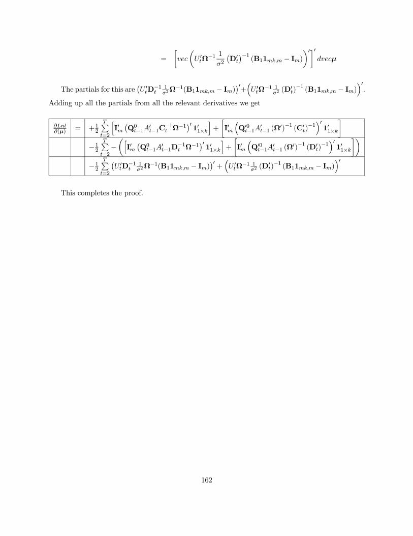
=
·vec
µU 0tΩ
−1 1σ2¡D0t
¢−1(B11mk,m − Im)
¶0¸0dvecµ
The partials for this are¡U 0tD
−1t
1σ2Ω−1(B11mk,m − Im)
¢0+³U 0tΩ−1
1σ2(D0
t)−1 (B11mk,m − Im)
´0.
Adding up all the partials from all the relevant derivatives we get
∂Lnl∂(µ) = +1
2
TPt=2
hI0m¡Q0t−1A0t−1C
−1t Ω
−1¢0 101×ki+ ·I0m ³Q00t−1A0t−1 (Ω0)−1 (C0t)−1´0 101×k¸−12
TPt=2−µhI0m¡Q0t−1A0t−1D
−1t Ω
−1¢0 101×ki+ ·I0m ³Q00t−1A0t−1 (Ω0)−1 (D0t)−1´0 101×k¸
−12TPt=2
¡U 0tD
−1t
1σ2Ω−1(B11mk,m − Im)
¢0+³U 0tΩ−1 1σ2 (D
0t)−1 (B11mk,m − Im)
´0This completes the proof.
162

Vita
Maria S. Heracleous was born on August 9, 1974, in Nicosia, Cyprus. In 1993 she went to the
London School of Economics to pursue studies in economics. After completing her Bachelor of
Science degree in Econometrics and Mathematical Economics, in July 1996, she continued with
graduate studies at the London School of Economics. She completed her Master of Science degree
in Econometrics and Mathematical Economics in July 1997 and returned to Cyprus, where she
worked with the firm ACNielsen and the University of Cyprus. In August 1998 she joined the Ph.D.
program in Economics at Virginia Polytechnic Institute and State University. She completed the
requirements for her Ph.D. in Economics in August 2003.
163
Recommended