VISUAL SALIENCY IN VIDEO COMPRESSION AND
TRANSMISSION
by
Hadi Hadizadeh
M.Sc., Iran University of Science and Technology, 2008
B.Sc., Shahrood University of Technology, 2005
a Thesis submitted in partial fulfillment of
the requirements for the degree of
Doctor of Philosophy
in the
School of Engineering Science
Faculty of Applied Sciences
c© Hadi Hadizadeh 2013
SIMON FRASER UNIVERSITY
Spring 2013
All rights reserved. However, in accordance with the Copyright Act of Canada, this work
may be reproduced, without authorization, under the conditions for Fair
Dealing. Therefore, limited reproduction of this work for the purposes of private
study, research, criticism, review and news reporting is likely to be in accordance
with the law, particularly if cited appropriately.

APPROVAL
Name: Hadi Hadizadeh
Degree: Doctor of Philosophy
Title of Thesis: Visual Saliency in Video Compression and Transmission
Examining Committee: Dr. Andrew Rawicz
Chair, Professor, School of Engineering Science
Dr. Ivan V. Bajic, Senior Supervisor,
Associate Professor, School of Engineering Science
Dr. Parvaneh Saeedi, Supervisor,
Associate Professor, School of Engineering Science
Dr. Jie Liang, Supervisor,
Associate Professor, School of Engineering Science
Dr. Rodney G. Vaughan, Internal Examiner,
Professor, School of Engineering Science
Dr. Zhou Wang, External Examiner,
Associate Professor, Electrical and Computer Engi-
neering, University of Waterloo
Date Approved: April 18, 2013
ii

iii

Abstract
This dissertation explores the concept of visual saliency—a measure of propensity for draw-
ing visual attention—and presents various novel methods for utilization of visual saliency
in video compression and transmission. Specifically, a computationally-efficient method for
visual saliency estimation in digital images and videos is developed, which approximates
one of the most well-known visual saliency models. In the context of video compression, a
saliency-aware video coding method is proposed within a region-of-interest (ROI) video cod-
ing paradigm. The proposed video coding method attempts to reduce attention-grabbing
coding artifacts and keep viewers’ attention in areas where the quality is highest. The
method allows visual saliency to increase in high quality parts of the frame, and allows
saliency to reduce in non-ROI parts. Using this approach, the proposed method is able to
achieve the same subjective quality as competing state-of-the-art methods at a lower bit rate.
In the context of video transmission, a novel saliency-cognizant error concealment method
is presented for ROI-based video streaming in which regions with higher visual saliency
are protected more heavily than low saliency regions. In the proposed error concealment
method, a low-saliency prior is added to the error concealment process as a regularization
term, which serves two purposes. First, it provides additional side information for the de-
coder to identify the correct replacement blocks for concealment. Second, in the event that a
perfectly matched block cannot be unambiguously identified, the low-saliency prior reduces
viewers’ visual attention on the loss-stricken regions, resulting in higher overall subjective
quality. During the course of this research, an eye-tracking dataset for several standard
video sequences was created and made publicly available. This dataset can be utilized to
test saliency models for video and evaluate various perceptually-motivated algorithms for
video processing and video quality assessment.
iv

To my lovely parents and family
v

Acknowledgements
I am thankful to many people for helping me during my Ph.D. program at Simon Fraser
University (SFU). Without their help, I would not be able to complete my program.
First and foremost, I wish to express my sincere gratitude and appreciation to my senior
supervisor, Prof. Ivan V. Bajic, for his persistent support and guidance during my doctoral
work. I would like to thank him for allowing me the freedom to explore my research and
industrial interests, with continual understanding, encouragement, and intellectual support.
I have learned a lot from him during my Ph.D. years. Many of his brilliant ideas have become
the very foundation of the present dissertation. He was the first person who introduced me
to the concept of visual saliency. I will always remain thankful and grateful to him.
I would also like to thank my supervisor, Prof. Parvaneh Saeedi. She was one of my
main motivations for coming to SFU for my graduate studies. During the past four years, I
had a very good and memorable collaboration with her on different research projects about
digital image processing, and it was my great honor and pleasure working with her.
I am also grateful to Prof. Jie Liang. I have learned a lot about image and video com-
pression and digital signal processing from his very valuable, up-to-date, and comprehensive
courses. He has a very nice personality, and it was my pleasure working with him at the
Multimedia Communications Laboratory at SFU.
I am very thankful to Prof. Zhou Wang for accepting to be my external examiner, and
taking his valuable time to read my thesis. I am also very grateful to my internal examiner,
Prof. Rodney G. Vaughan, for the patience to read my thesis. I like to thank Prof. Andrew
Rawicz for chairing my defence.
I feel very privileged to get to know many of my good friends at Multimedia Communi-
cations Laboratory at SFU. I am especially grateful to Dr. Yue-meng Chen, Dr. Jing Wang,
Dr. Upul Samarawickrama, Ali Amiri, Mahtab Torki, Duncan Chan, Carl Qian, Xiaonan
vi

Ma, Choong-hoon Kwak, Sohail Bahmani, Hossein Khatoonabadi, Homa Eghbali, Victor
Mateescu, and Hanieh Khalilian for all the entertainment and caring they provided.
Lastly, and most importantly, I would like to express my great and special gratitude
to my lovely parents and family who continuously encouraged and supported me during
the difficult times of being away from home. In particular, I would like to dedicate this
dissertation to my lovely father who has always been my inspiration.
vii

Contents
Approval ii
Partial Copyright License iii
Abstract iv
Dedication v
Acknowledgements vi
Contents viii
List of Tables xii
List of Figures xiii
List of Symbols xv
List of Acronyms xviii
1 Introduction 1
1.1 Visual Attention . . . . . . . . . . . . . . . . . . . . . . . . . . . . . . . . . . 1
1.2 Contributions . . . . . . . . . . . . . . . . . . . . . . . . . . . . . . . . . . . . 4
1.2.1 An eye-tracking database for a number of standard video sequences . 4
1.2.2 Computationally-efficient visual saliency models . . . . . . . . . . . . 4
1.2.3 Saliency-aware video compression . . . . . . . . . . . . . . . . . . . . . 5
1.2.4 Saliency-cognizant video error concealment . . . . . . . . . . . . . . . 5
1.2.5 Scholarly publications . . . . . . . . . . . . . . . . . . . . . . . . . . . 6
viii
1.3 Organization . . . . . . . . . . . . . . . . . . . . . . . . . . . . . . . . . . . . 7
2 Visual Attention and Its Computational Models 9
2.1 Mechanisms of attentional deployment . . . . . . . . . . . . . . . . . . . . . . 10
2.2 Computational models of visual attention . . . . . . . . . . . . . . . . . . . . 12
2.2.1 The Itti-Koch-Niebur model . . . . . . . . . . . . . . . . . . . . . . . . 18
2.2.2 The Itti-Baldi model . . . . . . . . . . . . . . . . . . . . . . . . . . . . 19
3 Eye-Tracking Data 21
3.1 Existing eye-tracking data sets . . . . . . . . . . . . . . . . . . . . . . . . . . 22
3.1.1 Existing eye-tracking datasets for static images . . . . . . . . . . . . . 22
3.1.2 Existing eye-tracking datasets for video . . . . . . . . . . . . . . . . . 23
3.2 Our database . . . . . . . . . . . . . . . . . . . . . . . . . . . . . . . . . . . . 25
3.2.1 Video sequences . . . . . . . . . . . . . . . . . . . . . . . . . . . . . . 25
3.2.2 Eye tracker . . . . . . . . . . . . . . . . . . . . . . . . . . . . . . . . . 25
3.2.3 Eye-tracking data collection . . . . . . . . . . . . . . . . . . . . . . . . 31
3.2.4 Gaze data visualization . . . . . . . . . . . . . . . . . . . . . . . . . . 32
3.2.5 Database location, structure and accessibility . . . . . . . . . . . . . . 33
3.3 Results . . . . . . . . . . . . . . . . . . . . . . . . . . . . . . . . . . . . . . . . 35
3.3.1 Congruency of first vs. second viewing . . . . . . . . . . . . . . . . . . 35
3.3.2 Accuracy of two popular visual attention models . . . . . . . . . . . . 37
3.4 Conclusions . . . . . . . . . . . . . . . . . . . . . . . . . . . . . . . . . . . . . 41
4 Computationally-Efficient Saliency Estimation 44
4.1 Background . . . . . . . . . . . . . . . . . . . . . . . . . . . . . . . . . . . . . 44
4.2 A convex approximation to IKN saliency . . . . . . . . . . . . . . . . . . . . . 46
4.3 Global motion-compensated saliency . . . . . . . . . . . . . . . . . . . . . . . 52
4.4 Accuracy . . . . . . . . . . . . . . . . . . . . . . . . . . . . . . . . . . . . . . 53
4.4.1 Assessment of the convex approximation to IKN saliency . . . . . . . 53
4.4.2 Evaluating GMC saliency estimation . . . . . . . . . . . . . . . . . . . 57
4.5 Computational Complexity . . . . . . . . . . . . . . . . . . . . . . . . . . . . 63
4.5.1 Complexity of the proposed convex approximation to IKN saliency . . 64
4.5.2 Complexity of the proposed GMC saliency estimation method . . . . . 67
4.6 Conclusions . . . . . . . . . . . . . . . . . . . . . . . . . . . . . . . . . . . . . 69
ix

5 Saliency-Aware Video Compression 70
5.1 Rate-distortion optimization in H.264/AVC . . . . . . . . . . . . . . . . . . . 72
5.2 Saliency-aware video compression . . . . . . . . . . . . . . . . . . . . . . . . . 74
5.2.1 Macroblock QP selection . . . . . . . . . . . . . . . . . . . . . . . . . 74
5.2.2 RDO mode decision . . . . . . . . . . . . . . . . . . . . . . . . . . . . 75
5.2.3 Statistical modeling of transformed residuals . . . . . . . . . . . . . . 77
5.2.4 The rate model . . . . . . . . . . . . . . . . . . . . . . . . . . . . . . . 78
5.2.5 The distortion models . . . . . . . . . . . . . . . . . . . . . . . . . . . 79
5.2.6 A closed-form expression for λRi. . . . . . . . . . . . . . . . . . . . . 80
5.3 Experimental results . . . . . . . . . . . . . . . . . . . . . . . . . . . . . . . . 81
5.3.1 Objective quality assessment . . . . . . . . . . . . . . . . . . . . . . . 81
5.3.2 Subjective evaluation . . . . . . . . . . . . . . . . . . . . . . . . . . . 84
5.4 Conclusions . . . . . . . . . . . . . . . . . . . . . . . . . . . . . . . . . . . . . 88
6 Saliency-Cognizant Video Error Concealment 89
6.1 Related work . . . . . . . . . . . . . . . . . . . . . . . . . . . . . . . . . . . . 91
6.1.1 RECAP video transmission system . . . . . . . . . . . . . . . . . . . . 93
6.1.2 Overview of the error concealment method from [1] . . . . . . . . . . . 94
6.2 The proposed error concealment method . . . . . . . . . . . . . . . . . . . . . 96
6.2.1 Problem formulation . . . . . . . . . . . . . . . . . . . . . . . . . . . . 96
6.2.2 The saliency operator S(N (X)) . . . . . . . . . . . . . . . . . . . . . . 98
6.2.3 Solving the error concealment problem . . . . . . . . . . . . . . . . . . 99
6.3 Computational complexity . . . . . . . . . . . . . . . . . . . . . . . . . . . . . 100
6.3.1 Computational complexity of the proposed method . . . . . . . . . . . 100
6.3.2 Comparison with the method from [1] . . . . . . . . . . . . . . . . . . 104
6.4 Experimental results . . . . . . . . . . . . . . . . . . . . . . . . . . . . . . . . 105
6.4.1 Objective quality assessment . . . . . . . . . . . . . . . . . . . . . . . 105
6.4.2 Subjective evaluation . . . . . . . . . . . . . . . . . . . . . . . . . . . 107
6.5 Conclusions . . . . . . . . . . . . . . . . . . . . . . . . . . . . . . . . . . . . . 110
7 Conclusions and Future Directions 112
7.1 Summary of contributions . . . . . . . . . . . . . . . . . . . . . . . . . . . . . 112
7.2 Future directions . . . . . . . . . . . . . . . . . . . . . . . . . . . . . . . . . . 114
x

Appendices 116
Appendix A 117
Bibliography 121
xi

List of Tables
3.1 Measurement error on all ten subjects. . . . . . . . . . . . . . . . . . . . . . . 30
3.2 Measurement error on subjects with/without contact lenses. . . . . . . . . . . 30
3.3 Measurement error before and after watching the video clip. . . . . . . . . . . 30
3.4 Average distance between gaze locations . . . . . . . . . . . . . . . . . . . . . 35
3.5 Average accuracy score for predicting gaze . . . . . . . . . . . . . . . . . . . . 39
3.6 Average accuracy score for the uniformly spread saliency . . . . . . . . . . . . 40
3.7 Average AUC score for predicting gaze . . . . . . . . . . . . . . . . . . . . . . 42
4.1 Average AUC scores of the spatial IKN saliency . . . . . . . . . . . . . . . . . 54
4.2 Average symmetric KLD between the IKN saliency . . . . . . . . . . . . . . . 58
4.3 Average AUC score of the IKN model and the proposed approximation . . . 58
4.4 The proposed GMC saliency estimation versus IKN-MA . . . . . . . . . . . . 60
4.5 Comparing the proposed GMC saliency estimation method . . . . . . . . . . 61
4.6 Comparing the proposed GMC saliency estimation method . . . . . . . . . . 62
4.7 Comparing the proposed GMC saliency estimation method . . . . . . . . . . 62
4.8 Comparing the proposed GMC saliency detection method . . . . . . . . . . . 65
5.1 Comparing the proposed video compression method . . . . . . . . . . . . . . 85
5.2 Comparing various methods with conventional RDO . . . . . . . . . . . . . . 86
5.3 Subjective comparison of the proposed video compression . . . . . . . . . . . 88
6.1 Comparing the proposed error concealment method with RECAP . . . . . . . 106
6.2 Comparing the proposed error concealment method with RECAP . . . . . . . 106
6.3 Subjective comparison of the proposed method against RECAP. . . . . . . . 109
6.4 Subjective comparison of the proposed method against the method from [1]. . 109
xii

List of Figures
2.1 A schematic diagram of the IKN model [2]. . . . . . . . . . . . . . . . . . . . 20
3.1 A photo of the Locarna eye tracker. . . . . . . . . . . . . . . . . . . . . . . . 26
3.2 A photo of the eye-tracking setup. . . . . . . . . . . . . . . . . . . . . . . . . 26
3.3 The dot pattern used for calibration. . . . . . . . . . . . . . . . . . . . . . . . 28
3.4 The dot pattern used for testing. . . . . . . . . . . . . . . . . . . . . . . . . . 28
3.5 The relative position of the test dots with respect to the calibration dots. . . 29
3.6 Two samples of the pupil detected by Pt-Mini . . . . . . . . . . . . . . . . . . 31
3.7 Heat map visualization of City for the first viewing. . . . . . . . . . . . . . . 34
3.8 Gaze plot visualization comparing first and second viewing of City. . . . . . . 34
3.9 Average distance (in pixels) between gaze locations . . . . . . . . . . . . . . . 37
3.10 Average ROC curves of the IKN and IB models . . . . . . . . . . . . . . . . . 43
4.1 A simple example showing the effect of spectral leakage . . . . . . . . . . . . 48
4.2 A simple example showing the effect of spectral leakage . . . . . . . . . . . . 48
4.3 Wiener coefficients for a 16× 16 block for two common resolutions. . . . . . . 50
4.4 Sample images from the Toronto data set (left) along with their IKN . . . . . 56
4.5 Average ROC curves of IKN-MA and the proposed convex approximation . . 59
4.6 Model ranking based on the number of top performances. . . . . . . . . . . . 63
4.7 A frame from City : (a) original frame . . . . . . . . . . . . . . . . . . . . . . 64
4.8 Average ROC curves of IKN-FA and the Proposed GMC Saliency models . . 66
5.1 A plot of EWPSNR versus rate for Foreman. . . . . . . . . . . . . . . . . . . 83
5.2 A plot of EWPSNR versus rate for Tempete. . . . . . . . . . . . . . . . . . . 84
6.1 Overview of RECAP packet loss recovery system. . . . . . . . . . . . . . . . . 93
xiii

6.2 An illustration of the missing block X . . . . . . . . . . . . . . . . . . . . . . 100
6.3 Visual samples for RECAP as well as the proposed method . . . . . . . . . . 111
A.1 Various possible cases for N (X) . . . . . . . . . . . . . . . . . . . . . . . . . . 118
xiv

List of Symbols
F A video frame
X A block or macroblock in the current frame
X0 The co-located block or macroblock in the previous frame
Xi The i-th macroblock in the frame
S(X) The saliency of X
Sgmc(X) The global motion compensated saliency of X
Sspatial(X) The spatial saliency of X
Stemporal(X) The temporal saliency of X
Smotion(X) The motion saliency of X
N (X) A spatial neighborhood around X
ZX The 2-D DCT of X
ZX(j, l) The (j, l)-th DCT coefficient of X
ZWX The Wiener-filtered of ZX
H(ω) The transfer function of the Wiener filter in the frequency domain
SS(ω) The power spectral density of the signal
SV (ω) The power spectral density of the noise
H The DCT-domain Wiener filter
H(j, l) The (j, l)-th coefficient of H
Q The residual block
Q The quantization step size
QP The quantization parameter
QPf The quantization parameter of frame f
QPi The quantization parameter of the i-th macroblock
Qi The quantization step size of the i-th macroblock
xv

J The Lagrangian cost function
ψ coding mode
DMSE The MSE distortion
Dsal The saliency distortion
λR The frame-level Lagrange multiplier
R The rate
s The average saliency within the current frame
λRiThe Lagrange multiplier of the i-th macroblock
λSiThe saliency distrotion weight of the i-th macroblock
λS The general saliency distrotion weight
Xi(ψ|Qi) The macroblock encoded under coding mode ψ with Qi
λ The Laplace parameter
Y The transformed residual
Yi The transformed residual of the i-th macroblock
σY The standard deviation of Y
σ2Yi(j, l) The variance of the (j, l)-th DCT coefficient of Yi
σ2ri The variance of the residual signal of Xi
ρi The correlation coefficient of the residual signal of Xi
A(ψ) The N ×N transform matrix of coding mode ψ
K(ψ) The covariance matrix of coding mode ψ
hi(j, l) The entropy of the (j, l)-th DCT coefficient
Fx,y The pixel value at location (x, y) in frame F
F′
x,y The pixel value at location (x, y) in encoded frame F′
W The width of the frame (pixels)
H The height of the frame (pixels)
wx,y The value of the Gaussian weight function at location (x, y)
σx The width of the Gaussian weight function
σy The height of the Gaussian weight function
D The down-sampling matrix
w The width of a spatial window
h The height of a spatial window
vec(.) The vectorization operator
I The idenity matrix
xvi

T The thumbnail block
L A low-pass FIR filter
L The high-pass complement of L
Rk The k-th RECAP candidate
K The total number of RECAP candidates
d The distance between the current frame and the reference frame
Xe The extended version of X
M A p×m binary matrix
N A m× p binary matrix
Nt The transpose of matrix N
Z(.) The matrix extension operator
ds The down-sampling factor
Nb The width or height of a block
p The width or height of a spatial neighborhood
ζ(.) The complexity operator
xvii

List of Acronyms
1-D One-Dimensional
2AFC Two Alternative Forced Choice
2-D Two-Dimensional
AUC Area Under Curve
AVC Advanced Video Coding
BD Bjontegaard Delta
CIF Common Interchange Format
CRF Conditional Random Field
CSF Contrast Sensitivity Function
DBN Dynamic Bayesian Network
DCT Discrete Cosine Transform
DFT Discrete Fourier Transform
DSCQS Double Stimulus Continuous Quality Scale
EWPSNR Eye-tracking-weighted Peak Signal to Noise Ratio
FA FancyOne saliency normalization operator
FBA Feature Based Attention
FEC Forward Error Correction
FIT Feature Integration Theory
FJND Foveated Just-Noticeable Difference
GBVS Graph Based Visual Saliency
GMC Global Motion Compensation
GMC-MV Global Motion-Compensated Motion Vector
GOP Group of Pictures
HMM Hidden Markov Model
xviii
HR High Resolution
HVS Human Visual System
IB Itti-Baldi
IKN Itti-Koch-Niebur
JM Joint Model reference software
KL Kullback-Leibler
KLD Kullback-Leibler Divergence
LR Low Resolution
MA MaxNorm saliency normalization operator
MB Macroblock
MOS Mean Opinion Score
MSE Mean Squared Error
MV Motion Vector
PDF Probability Density Function
PQFT Phase Spectrum of Quaternion Fourier Transform
PSNR Peak Signal to Noise Ratio
QP Quantization Parameter
RD Rate-Distortion
RDO Rate-Distortion Optimization
RECAP Receiver Error Concealment using Acknowledge Preview
ROI Region of Interest
ROC Receiver Operating Characteristic
SAD Sum of Absolute Differences
SSIM Structural Similarity Index
SVD Singular Value Decomposition
SVM Support Vector Machine
UEP Unequal Error Protection
VA Visual Attention
VAGBA Visual Attention Guided Bit Allocation
VQM Video Quality Metric
WTA Winner Take All
xix

Chapter 1
Introduction
1.1 Visual Attention
It is well-known that due to the limited capacity of the brain, only a small amount of vi-
sual information that is received at the retina of our eyes can reach the latter processing of
the brain and impact our conscious awareness [3]. Visual attention provides a mechanism
for selection of particular aspects of a visual scene that are most relevant to our ongoing
behaviour while eliminating interference from irrelevant visual data in the background. Per-
haps, one of the earliest definitions of attention was provided by William James in 1890 in
his textbook “Principles of Psychology” [4]:
“Everyone knows what attention is. It is the taking possession by the mind, in clear and
vivid form, of one out of what seem several simultaneously possible objects or trains of
thought. Focalization, concentration, of consciousness are of its essence. It implies
withdrawal from some things in order to deal effectively with others.”
Over the last decades, visual attention (VA) has been studied intensely, and research has
been conducted to understand the deployment mechanisms of visual attention. According
to the current knowledge, the deployment of visual attention is believed to be driven by
“visual saliency,” that is, the characteristics of visual patterns or stimuli, such as a red
flower in a green grass field, that makes them stand out from their surroundings and draw
our attention in an automatic and rapid manner. Various computational models of visual
attention have then been developed based on this belief for different applications such as
robotics, navigation, image and video processing, and so on [5], [6]. Such computational
1

CHAPTER 1. INTRODUCTION 2
models of human visual attention are commonly referred to as visual saliency models, and
their goal is to predict where people are likely to look in a visual scene.
The perceptual coding of video using visual saliency models has been recently recognized
as an increasingly promising approach to achieve high-performance video compression [5].
The rationale behind most of the existing saliency-based video coding methods is to encode
a small area around the predicted gaze locations with higher quality compared to other
less visually important or interesting regions. Such a spatial prioritization is supported by
the fact that only a small region of several degrees of visual angle (i.e., the fovea) around
the center of gaze is perceived with high spatial resolution due to the highly nonuniform
distribution of photoreceptors on the human retina. Therefore, the idea is that it may not
be necessary to encode each video frame with a uniform quality because human observers
will perceive only a very small portion of each frame around their gaze locations, which
we may call regions-of-interest (ROIs). Hence, based on these principles, ROIs should be
encoded with a higher quality compared to the rest of the frame. The hope is that one may
save bits while achieving the same subjective quality as a conventional approach that grants
the same quality across the frame.
In practice, the encoding prioritization can be performed in several ways. In one popular
approach, the compression ratio is decreased in ROI parts of the frame whereas it is increased
in non-ROI parts. Using this approach, the overall compressed video size may decrease as
ROI parts of the frame usually constitute a small portion of the frame, so the extra bits spent
on their encoding are more than offset by the savings in non-ROI parts. Another approach
is to apply a so-called “foveation filter” [5] to the video content before the encoding process.
The foveation filter spatially blurs the video frame, increasingly with distance from ROI
parts of the frame. Hence, due to the loss of higher spatial frequencies in non-ROI parts
after applying the foveation filter, non-ROI parts take fewer bits to encode, and so bit rate
savings can be achieved. In another, more sophisticated approach [7], the prioritization may
be performed by a progressive or scalable scheme, for example, by delivering priority regions
first or continuously scaling the video quality depending on a given transmission bandwidth
or bit budget. Such encoding schemes are generally referred to as ROI-based video coding
methods.
Although ROI-based video coding methods can achieve high compression, the selection of
ROI parts remains an open and challenging problem. In recent years, several advances have
been achieved to tackle this problem with two approaches. The first approach involves the

CHAPTER 1. INTRODUCTION 3
use of an eye-tracking device to interactively record eye gaze position of a human observer
on the receiving side in order to find the ROI in real time [8], [9]. A foveation filter is
then applied on the source video signal on the transmitting side, taking the detected ROI
into account, and the foveated video is transmitted to the receiver. In a variant of this
approach, gaze locations of a number of observers watching the same video are measured
by an eye-tracking device off-line, and their union is treated as the ROI [10]. Although this
approach can provide a good estimate of the ROI, it is neither generic nor cost-effective.
It is very time consuming as it requires an eye-tracking setup and collecting and training
various observers for every video to be compressed.
Rather than deducing ROI based on measurement, the second approach instead relies
on visual saliency models for finding ROI [5]. Here, ROIs are declared to be the parts of
the frame where viewers are most likely to focus their visual attention, according to the
employed saliency model. This general-purpose and automatic approach has the advantage
that it does not require human interaction, and so it is practical and cost-effective. The
downside, of course, is that it is only as accurate as the saliency model it relies on.
ROI-based processing can also be employed in the context of video transmission to
combat the effects of transmission channel errors. For instance, ROI parts of the frame
can be protected heavily (e.g., by using stronger channel codes) than non-ROI parts of the
frame [11], so that in the case of channel errors or losses, important parts of the frame can
still be decoded correctly. In this case, also, ROI could be detected either based on direct
eye-tracking measurement or based on visual saliency models.
Despite the increasing popularity of saliency-based video compression and transmission
methods, such approaches are still immature. Integrating a complex saliency model within
another video processing task can be cumbersome. The main goal of this dissertation is
to develop novel methods for better utilization of visual saliency in video compression and
transmission. For this purpose, we first develop an efficient approximation to a popular
visual saliency model that partially operates in the transform domain, and reuses some of
the data that is normally present in video compression. This reduces the computational
cost of estimating visual saliency and makes it easier to incorporate into various video
processing systems. We then utilize this approximation within a ROI-based framework for
efficient video compression and transmission.

CHAPTER 1. INTRODUCTION 4
1.2 Contributions
The main contributions of this research are as follows.
1.2.1 An eye-tracking database for a number of standard video sequences
The best way to test the accuracy of visual saliency models is to compare their predictions
with real eye-tracking data. Such data can also be used to evaluate various saliency-based
video processing algorithms. However, eye-tracking devices are still fairly expensive and are
not easily accessible to most researchers. To facilitate the development and testing of novel
perceptually-motivated algorithms and models of visual attention, we developed a pub-
licly available database of eye-tracking data, collected on a set of standard video sequences
that are frequently used in video compression, processing, and transmission simulations. A
unique feature of this database is that it contains eye-tracking data for both the first and
second viewings of the sequence. The dataset is described in [12], and will be discussed in
Chapter 3.
1.2.2 Computationally-efficient visual saliency models
Among the existing saliency models, the Itti-Koch-Niebur (IKN) saliency model [2] is the
most well-known and widely-used model. However, this bottom-up model of visual attention
is very complex as it requires multiresolution analysis of the input image or video in in various
feature channels such as intensity, color, and orientation. In this dissertation, we present
two computationally-efficient saliency models inspired by the IKN model. Both models are
described in Chapter 4.
The first proposed model is a convex approximation to the IKN saliency model. It
consists of two parts: spatial and temporal. The spatial part can be used to estimate
saliency in static images, whereas the temporal part in conjunction with the spatial part
can be utilized to estimate saliency in video. The model estimates saliency using the signal
energy in the Discrete Cosine Transform (DCT) domain, which makes it useful for saliency
estimation in DCT-based image and video processing tasks. This model was first introduced
in [13], and its application to video error concealment will be described in Chapter 6.
Although this model is slightly less accurate than the IKN model, it has several practical
advantages. First, its computational complexity is much lower than that of the IKN model,
making it attractive for real time implementation. Second, it is convex in the input data.
CHAPTER 1. INTRODUCTION 5
This means that when the saliency estimate produced by this model is linearly combined
with other convex measures (e.g., mean squared error), it results in a convex function,
which can lead to convex optimization formulations (and corresponding efficient solutions)
in various image and video processing tasks. One example is given in Chapter 6, where
this approximation is used to make a saliency-cognizant error concealment problem convex,
which in turn leads to an efficient solution.
The second proposed saliency model uses the convex approximation to the spatial IKN
model mentioned above, but improves the temporal saliency estimation via global motion
compensation [14]. We refer to this method as Global Motion-Compensated (GMC) saliency
estimation. Overall, this method is not convex, but is more accurate than the IKN model
on certain sequences with camera motion. This method was first introduced in [15], and
will be used in saliency-aware video compression in Chapter 5.
1.2.3 Saliency-aware video compression
As stated earlier, in ROI-based video coding, ROI parts of the frame are encoded with higher
quality than non-ROI parts. At low bit rates, such encoding may produce attention-grabbing
coding artifacts, which may draw viewers attention away from ROI, thereby degrading visual
quality. In this dissertation, we present a saliency-aware video compression method for
ROI-based video coding. The proposed method aims at reducing salient coding artifacts in
non-ROI parts of the frame in order to keep users attention on ROI. Further, the method
allows saliency to increase in high quality parts of the frame, and allows saliency to reduce
in non-ROI parts. The ideas behind this approach are described in [16] and [15], and will
be discussed in Chapter 5.
1.2.4 Saliency-cognizant video error concealment
Visual saliency can be an effective tool in dealing with errors and losses in video transmission,
and hiding their effects from the viewers. In this dissertation, we add a low-saliency prior
to the under-determined problem of error concealment as a regularization term. There are
multiple reasons for doing so. First, in ROI-based video transmission, low-saliency prior
is likely the correct side information for the lost block and helps the client to identify the
correct replacement block for concealment. Second, in the event that a perfectly matched
block cannot be identified, the low-saliency prior reduces viewers’ visual attention on the
CHAPTER 1. INTRODUCTION 6
loss-stricken region, resulting in higher overall subjective quality. In a way, the low-saliency
prior tries to make error concealment live up to its name by attempting to hide damaged
blocks from viewers attention. It is the low-saliency prior that puts concealment into error
concealment – the rest is just interpolation. To the best of our knowledge, our work is the
first to apply saliency analysis for error concealment in video transmission. This approach
has been described in [1] and [13], and will be discussed in Chapter 6.
1.2.5 Scholarly publications
My research efforts during my Ph.D. program have resulted in the following scholarly pub-
lications. Please note that the material in this dissertation is only related to several of the
most recent ones, specifically journal papers 1-3, and conference papers 3 and 5.
Journal Papers:
1. H. Hadizadeh and I. V. Bajic, “Saliency-aware video compression,” submitted to IEEE
Trans. Image Processing, Feb. 2013.
2. H. Hadizadeh, I. V. Bajic, and G. Cheung, “Video error concealment using a computation-
efficient low saliency prior,” submitted to IEEE Trans. Multimedia, Dec. 2012. Cur-
rently under revision. (Invited Paper)
3. H. Hadizadeh, M. J. Enriquez, and I. V. Bajic, “Eye-tracking database for a set of
standard video sequences,” IEEE Trans. Image Processing, vol. 21, no. 2, Feb. 2012.
4. H. Hadizadeh and I. V. Bajic, “Rate-distortion optimized pixel-based motion vector
concatenation for reference picture selection,” IEEE Trans. Circuits Syst. Video
Technol., vol. 21, no. 8, pp. 1139-1151, Aug. 2011. (Among top 25 most download
papers from this journal in August 2011)
5. H. Hadizadeh and I. V. Bajic, “Burst loss resilient packetization of video,” IEEE
Trans. Image Processing, vol. 20, no. 11, pp. 3195-3206, Nov. 2011.
Conference Papers:
1. V. A. Mateescu, H. Hadizadeh, and I. V. Bajic, “Evaluation of several visual saliency
models in terms of gaze prediction accuracy on video,” Proc. IEEE Globecom’12
Workshop: QoEMC, pp. 1304-1308, Anaheim, CA, Dec. 2012.

CHAPTER 1. INTRODUCTION 7
2. H. Hadizadeh, M. Fatourechi, and I. V. Bajic, “An automatic lyrics recognition system
for digital videos,” presented at IEEE MMSP’12 (On-going Work Track), Banff, AB,
Sep. 2012.
3. H. Hadizadeh, I. V. Bajic, and G. Cheung, “Saliency-cognizant error concealment
in loss-corrupted streaming video,” Proc. IEEE ICME’12, pp. 73-78, Melbourne,
Australia, Jul. 2012. (Best Paper Runner-up)
4. H. Hadizadeh, I. V. Bajic, P. Saeedi, and S. Daly, “Good-looking green images,” Proc.
IEEE ICIP’11, pp. 3177-3180, Brussels, Belgium, Sep. 2011.
5. H. Hadizadeh and I. V. Bajic, “Saliency-preserving video compression,” presented at
IEEE AVCC, in conjunction with IEEE ICME’11, Barcelona, Spain, Jul. 2011.
6. H. Hadizadeh and I. V. Bajic, “Pixel-based motion vector concatenation for reference
picture selection,” Proc. IEEE ICME’10, pp. 209-213, Singapore, July 2010.
7. H. Hadizadeh, S. Muhaidat, and I. V. Bajic, “Impact of imperfect channel estimation
on the performance of inter-vehicular cooperative networks,” presented at 25th Queen’s
Biennial Symposium on Communications (QBSC’10), Kingston, ON, Canada, May
2010.
8. H. Hadizadeh and I. V. Bajic, “Burst loss resilient packetization of video,” Proc. IEEE
ICC’10, Cape Town, South Africa, May 2010.
9. H. Hadizadeh and I. V. Bajic, “NAL-SIM: An interactive simulator for H.264/AVC
video coding and transmission,” presented at Proc. IEEE CCNC’10, Las Vegas, NV,
USA, Jan. 2010.
1.3 Organization
This dissertation is organized as follows. In Chapter 2, we present a brief description of the
concept of visual attention and its deployment mechanisms. We also present a survey of
several existing computational models of visual attention. In particular, we briefly describe
two popular saliency models, the Itti-Koch-Neibur (IKN) model [2] and the Itti-Baldi (IB)
model [17]. In Chapter 3, we present our eye-tracking database for a number of standard
video sequences. Two novel computationally-efficient visual saliency models are presented

CHAPTER 1. INTRODUCTION 8
in Chapter 4. Our proposed saliency-aware video compression method is presented and
evaluated in Chapter 5. The proposed saliency-cognizant error concealment method for
video streaming is described in Chapter 6. Finally, the conclusions and future directions are
given in Chapter 7.

Chapter 2
Visual Attention and Its
Computational Models
It is known that the brain in primates has a “massively parallel” computational structure [3].
However, similar to any physical system, the processing and computational resources of
the brain are limited. Every time that we open our eyes to the world, we encounter an
overwhelming amount of visual information. It has been estimated that the amount of visual
information coming to our visual system is on the order of 108 bits per second, which far
exceeds the processing power and computational capacity of our brain [3]. Nevertheless, we
are able to experience an almost effortless understanding of our visual world. This requires
separating relevant information from irrelevant data in a preferential and serial manner.
Such a process is operationalized by the mechanisms of “visual attention” [3, 18], which
allows us to break down the daunting problem of visual scene understanding into a rapid
series of computationally less demanding, localized visual analysis problems [19]. According
to [20], attention is the cognitive process of selectively concentrating on one aspect of the
environment while ignoring other irrelevant things. Attention has also been referred to as
the allocation of processing resources [20]. Hence, visual attention optimizes the use of our
visual system’s limited resources for gathering and processing the most relevant information
in a complex visual environment. In other words, visual attention turns our looking into
seeing [18].
The topic of visual attention is vast, and since 1980, the concept of visual attention has
been studied in several thousands of scientific papers with an increasingly growing rate [18],
9

CHAPTER 2. VISUAL ATTENTION AND ITS COMPUTATIONAL MODELS 10
[21], [22], [23], [3]. According to a recent review on visual attention [18], there are three
main types of visual attention: (1) spatial attention, which can be either overt (i.e., when
an observer moves his/her eyes to focus on a specific region in the visual scene) or covert
(i.e., when a person mentally focuses on another sensory stimuli different from the stimuli at
his/her current fixation); (2) feature-based-attention (FBA), which can be deployed covertly
to specific aspects (e.g., color, orientation or motion direction) of objects in the environment,
regardless of their location; (3) object-based attention in which attention is influenced or
guided by a specific object structure or the relevance between different objects in a visual
scene. At any given time, these three types of visual attention can co-exist [18]. For instance,
when waiting to meet a friend in a restaurant, we may direct our spatial attention to the
entrance door of the restaurant (i.e., where our friend is likely to appear), and deploy our
FBA to red objects, assuming that our friend is wearing a red shirt [18].
2.1 Mechanisms of attentional deployment
Interesting questions related to the concept of visual attention are how the selection of one
particular spatial location or object in a cluttered visual scene is performed, or where in a
visual scene, the visual attention is deployed? In other words, if our brain can process only
one region or object at a time, then how do we select the target of our attention? Many
studies have been conducted for finding answers to these questions. Much evidence has been
accumulated in favor of the following two principal beliefs about the mechanisms of visual
attention deployment: [3],[24],[25],[26], [6]
1. There is a “bottom-up,” fast, primitive, and stimulus-driven mechanism that biases
the observer towards selecting stimuli based on their “visual saliency.” Here, “visual
saliency” means how much a certain stimulus (e.g., a region or object) is distinct from
its surroundings in terms of visual attributes such as color, intensity, and orientation,
so that it stands out from its surroundings. According to this scene-driven mechanism,
visual attention is attracted towards visually salient locations in a seemingly effortless
and automatic manner. Based on this mechanism, a red flower in a green grass field
is visually salient due to its high color contrast, drawing visual attention towards
itself. The terms “salient” and “visual saliency” are often utilized in the context of
bottom-up modeling of visual attention [6].

CHAPTER 2. VISUAL ATTENTION AND ITS COMPUTATIONAL MODELS 11
2. A “top-down,” slow, voluntary and user-driven mechanism with variable selection
criteria that intentionally directs the visual attention towards specific locations or ob-
jects in the visual scene, regardless of their visual saliency. Such a task-dependent and
expectation-driven mechanism can modulate or even sometimes override the bottom-
up deployment of visual attention. For instance, if we want to find our misplaced
car keys, those keys (i.e., their color, shape, etc.) become the primary drivers of our
attention; other object in the room would have a hard time drawing our attention in
this case.
The bottom-up control of visual attention relies on the fact that the brain does not
process all parts of a visual scene equally well, but instead provides a selective prioritization
with strong neural responses to a few parts of the scene, and poor responses to everything
else. Several studies provide direct support for the idea that different visual stimuli in a
visual scene compete for activity to draw visual attention [27], [28], [3], [19]. Those parts
that are very different from their surroundings can elicit a strong neural response, and can
draw visual attention to themselves. They are said to be salient. Directing attention to
other, non-salient parts, is thought to require voluntary effort, which can be employed by
the top-down mechanism of visual attention [3].
The top-down cues are often determined by cognitive phenomena such as knowledge,
expectations, reward, tasks, and goals [6]. One of the most popular examples for showing
the effect of the top-down guidance of visual attention on the eye movements is from the
following experiment described in [29]. Subjects were asked to watch a scene showing a
room with a family and an unexpected visitor entering the room. Some subjects were
allowed to freely watch the scene, while others were asked questions such as “what are the
ages of the people in the room?” or “estimate the material circumstances of the family.”
The results of this experiment showed that the eye movements were considerably different
under each question, which suggests that a task can significantly affect the deployment of
attention. Several researchers have studied the role of the task in the deployment of visual
attention in natural environments, for tasks like driving, sandwich making, playing cricket,
and walking [30], [31], [32].

CHAPTER 2. VISUAL ATTENTION AND ITS COMPUTATIONAL MODELS 12
2.2 Computational models of visual attention
In the past 25 years, modeling visual attention has been a very active research area. Vari-
ous computational models of human visual attention (a.k.a. “saliency models”) have been
proposed in both the computer vision community and biological vision and neuroscience
community. The main goal of such models is to predict the target of visual attention in a
given visual scene, for example in a given image or video. In other words, their goal is to
predict where people are likely to look.
In the computer vision community, the design and development of the so-called “saliency
detectors” or “interest point detectors” has been a significant research objective in the past
decades. Various saliency detectors have been proposed and adopted in many computer
vision applications such as object tracking and recognition, robotics, image and video com-
pression, advertising, etc. The majority of such models are closely related to object detection
and feature extraction methods. Broadly speaking, the existing saliency detectors proposed
in the computer vision literature can be classified into the following three classes:
• In the first class, the saliency detection problem is formulated as the detection of spe-
cific visual attributes such as edges, corners, contours, blobs, structure-from-motion,
and so on [33], [34]. A prominent advantage of such bottom-up saliency detectors is
that they can be defined with an explicit mathematical formulation, and can be imple-
mented using efficient computational methods. A major drawback of such detectors,
however, is that they cannot be generalized well for object recognition problems, and
so they cannot provide useful information for the desired recognition task at hand.
For instance, consider a white egg on top of a tree branch. A saliency detector that
uses corner information will show a strong response to the highly textured tree branch,
but not to the plain egg, even though the egg may be salient.
• In the second class, the saliency is defined as a measure of “image complexity.” Several
image complexity measures have been proposed in this context. For instance, in [35],
the saliency is defined as the variance of Gabor filter responses in different orientation
and frequency bands. In [36], the absolute values of 2-D wavelet coefficients are used
a measure of saliency. In [37], the entropy of local intensity histograms in an image
is used for saliency detection. The main advantage of such models is that they can
detect several low-level image features in a unified and generic manner. However,
CHAPTER 2. VISUAL ATTENTION AND ITS COMPUTATIONAL MODELS 13
similar to the first class, their main drawback is that they cannot directly provide
useful information for the recognition task of interest.
• In the third class, the saliency detection problem is formulated as an object detection
and recognition problem. Hence, the models in this class can be considered as top-
down saliency detectors. Examples of such models include those proposed in [38], [39],
[40]. Several object detection approaches can be utilized by the models in this class.
For instance, the deformable part model proposed in [41] and the attentional cascade
of Viola and Jones [42] can be employed to achieve a very high detection accuracy for
several objects such as cars, faces, and persons. The main advantage of such models is
their superior performance for salient object detection, especially in cluttered scenes.
However, by their very nature, such models are application-specific and hence have a
limited application scope.
The main objection to the saliency detection models proposed in the computer vision
literature is that they are application-oriented and seldom have a connection to the bio-
logical architecture of the human visual system. The main goal of such models is not to
explain attentional behavior. Instead, the goal is usually to make a computer perform a
vision-related task with the same end result as a human, regardless of whether or not the
intermediate processing is performed in the same way as in human vision. While this is per-
fectly appropriate for application purposes, methods that shed light on the actual principles
of human vision may have greater scientific value.
In the biological vision community, both the neurophysiological and psychophysical prop-
erties of visual attention have been extensively studied, and several computational models
of human visual attention have been proposed. Most such models emphasize biological
plausibility, and their goal is to replicate what is known about the biology and the neural
architecture of the human visual attention mechanisms. With a few exceptions [29], [43], the
majority of such models have been proposed for the bottom-up mechanism of visual atten-
tion. The reason is that the bottom-up mechanism of visual attention is better understood
due to its reliance on low-level processing tasks, which are easier to measure and study.
Meanwhile, the top-down attention relies on higher-level tasks in the brain that are still
not well understood. Moreover, as we mentioned earlier, top-down cues are often related to
tasks, expectations, rewards, and current goals. Hence, they are application-specific, related
to context and prior knowledge, and therefore difficult to model.

CHAPTER 2. VISUAL ATTENTION AND ITS COMPUTATIONAL MODELS 14
The basis of many of existing attention models is the well-known “Feature Integration
Theory” (FIT) proposed by Treisman and Gelade [44]. This theory postulates which visual
features are important and how they are combined together to direct visual attention in
search tasks [6]. More explicitly, FIT states that “different features are registered early,
automatically and in parallel across the visual field, while objects are identified separately
and only at a later stage, which requires focused attention” [44]. Based on FIT, Koch and
Ullman [45] proposed a computational model to combine these features, and they introduced
the concept of a two-dimensional topographical “master saliency map” that represents the
saliency of various regions and objects in a given visual scene. They also proposed a winner-
take-all (WTA) neural network that selects the most salient locations in a given saliency
map. Competition among different neurons in this network results in a single winning
location that corresponds to the most salient region in the scene. The next most salient
region in the scene can be found by inhibition of the current most salient object using a
specific inhibition of return (IOR) operator. Using this mechanism, the system can predict
the next focus of visual attention in a serial fashion. Several systems were proposed to
implement the Koch and Ullman model for computing the saliency maps of digital static
images [46], [47]. The first comprehensive implementation of the model, however, was
developed by Itti et al. [2]. This system was designed in a biologically plausible manner in
the sense that it attempts to replicate the biological and neural processes involved in human
vision. Itti et al. applied their attention model to synthetic and natural scenes, and they
showed that their model’s predictions have a high correlation with real eye-tracking data in
free-viewing tasks, which verifies the effectiveness of their method for saliency detection in
digital images [2].
Although the majority of existing models of visual attention have been developed for
static images, there also exist several models for saliency detection in video [5], [48], [49],
[50], [6]. Almost all such models consist of a spatial component and a temporal compo-
nent, which distinguishes them from the purely spatial models for static images. Some of
the saliency detection methods for video use a motion and a flicker channel for temporal
saliency detection [5]. Other models attempt to capture the spatio-temporal features of a
video by more sophisticated methods. For instance, the method in [51] computes the tem-
poral saliency based on the motion contrast obtained from the homographic transformation
between successive video frames. In [52], the temporal saliency is estimated in an irregu-
larity detection framework by comparing the spatio-temporal patches of the video with a

CHAPTER 2. VISUAL ATTENTION AND ITS COMPUTATIONAL MODELS 15
learned dataset of expected spatio-temporal patches.
Following the seminal model by Itti et al. [2], many other bottom-up saliency models
were proposed in the literature based on FIT. All such models of visual attention share
three common components. The first component is the extraction of various low-level visual
features from a given input image or video signal. Inspired by the processing mechanism of
neurons in the primary visual cortex (V1) of the human brain and the feature integration
theory, these features include various simple visual attributes such as intensity or luminance
contrast, color opponency, orientation and motion [2]. The second common component is the
so-called “center-surround” mechanism by which contrast features are computed in different
feature channels [2], [17], [53]. The center-surround mechanism is supported by the neural
responses of the visual receptive fields of neurons in the lateral geniculate nucleus (LGN)
[54] and V1 cortex of the human brain. Typical visual neurons are most sensitive in a small
region of the visual field (the center), and inhibit the neural response to stimuli presented
in a broader region concentric with the center (the surround) [2]. Hence, such architectures
can detect locations that stand out from their surroundings. The third component is the
computation of a “master saliency map” by which the saliency of different locations in a
visual scene can be estimated.
According to a recent survey of visual attention models presented in [6], the existing com-
putational models of visual attention can be classified into the following general categories
based their mechanism of computing saliency:
• Cognitive Models: These models have been built based on psychological and neuro-
physiological findings and cognitive concepts. Many of the existing attention models
fall within this category, especially those that were developed in the biological and
neuroscience community. Notable (popular) models from this category are the Itti-
Koch-Niebur (IKN) model [2] and the model proposed by Le Meur et al. [55]. The
IKN model is the most popular and widely-cited attention model, and it has been the
basis for the development and benchmarking of many other attention models. Hence,
it can be considered as the representative bottom-up attention model. Due to its
importance, we briefly describe it in Section 2.2.1. The model proposed by Le Meur
et al. [55] is also a bottom-up model, and shares some common features with the IKN
model. The main difference between these two models is that the model of Le Meur et
al. uses several psychophysical properties of the human visual system (HVS) [56] such

CHAPTER 2. VISUAL ATTENTION AND ITS COMPUTATIONAL MODELS 16
as the luma and chroma contrast sensitivity functions (CSFs), multi-band frequency
decomposition, visual masking, and center-surround computations. It also uses the
temporal information so that it can be utilized for saliency detection in video as well.
In other words, the model in [55] is a spatio-temporal saliency model while the original
IKN model [2] is a spatial saliency model. However, in [5], several temporal features
such as motion and flicker were added to the IKN model, which enabled its use for
saliency detection in video.
• Bayesian Models: The models in this class are based on the Bayes’ theorem to capture
subjective aspects of sensory information under prior knowledge. More specifically, in
these models, the sensory information (e.g., detected features) are combined with
prior knowledge (e.g., scene context) in a probabilistic manner using the Bayes’ rule
to detect a salient region in a visual scene [6]. Several models within this category
are [17], [57], [58], [59], [60], [61]. A representative model in this category is the Itti-
Baldi (IB) model proposed in [17]. In this model, a Bayesian definition of surprise was
presented. In their definition, a surprising stimulus is the one that significantly alters
the prior beliefs of a Bayesian observer. To quantify the amount of surprise, they
used the Kullback-Leibler (KL) divergence [62] between posterior and prior beliefs. In
Section 2.2.2, we briefly describe the IB model.
• Decision Theoretic Models: The models in this category are based on the “discriminant
saliency hypothesis” [63], which states that saliency is a discriminant process, and
all saliency processes are optimal in a decision-theoretic sense, i.e., with minimum
probability of decision error. Under this framework, the saliency of each location in
the visual field is considered as the discriminant power of the image features with
respect to a classification problem that opposes a class of interest (i.e., the target)
to all other visual classes. Notable (popular) model in this category is the model
proposed by Gao and Vasconcelos [63].
• Information Theoretic Models: These models are developed based on the hypothesis
that perceptual systems are designed to maximize information collected from the en-
vironment, so that only the most relevant and informative parts of the visual field are
selected and the rest is discarded [6]. The idea behind such models is supported by the
biological evidence that the primate visual system is built on the principle of estab-
lishing a sparse representation of image statistics [53]. The notable (popular) model

CHAPTER 2. VISUAL ATTENTION AND ITS COMPUTATIONAL MODELS 17
in this category is the model proposed by Bruce and Tsotsos [53]. Their bottom-up
model is based on Shannon’s self-information measure for computing saliency of image
regions. In their formulation, saliency of a local image region is the information that
region conveys relative to its surroundings, based on the probability density functions
of various RGB features.
• Graphical Models: The attention models in this category consider eye movements as
stochastic time series. Since there are hidden variables influencing the eye movements,
graphical networks [64] such as Hidden Markov Models (HMM), Dynamic Bayesian
Networks (DBN), and Conditional Random Fields (CRF) have been used by such
models to predict eye fixations or movements. The well-known model in this category
is the Graph-Based Visual Saliency (GBVS) model proposed by Harel et al. [38].
In this model, similar to the IKN model, several feature maps are first created at
different scales. A fully-connected graph is then created over all grid locations of each
feature map. The weight between each pair of nodes in each graph is computed by
the similarity of the feature values of the two nodes, as well as their spatial distance.
The resulting graphs are then considered as Markov chains, and a random walker [64]
is used to find the equilibrium distribution of each graph. The obtained equilibrium
distributions are used to construct the master saliency map for a given image.
• Spectral Analysis Models: In these attention models, saliency is estimated in the spec-
tral (frequency) domain instead of the spatial (pixel) domain. The popular models in
this category are the spectral residual saliency model proposed by Hou and Zhang [65]
and the “Phase Spectrum of Quaternion Fourier Transform” (PQFT) model proposed
by Guo and Zhang [48]. The spectral residual saliency model in [65] was designed based
on the idea that statistical singularities in the amplitude of the Fourier spectrum of an
image may be responsible for salient regions. Hence, by finding such regions, one can
construct a saliency map of the scene. In the PQFT method, it was observed that the
phase spectrum of the Fourier transform can also be utilized for saliency prediction.
Based on this idea, a quaternion representation of a video was proposed in [48], and
it was used for spatio-temporal saliency detection.
• Pattern Classification Models: The models in this category employ machine learning
approaches for discovering the relation between image features and measured eye fixa-
tions. A popular model in this category is the model proposed by Kienzle et al. [66], in

CHAPTER 2. VISUAL ATTENTION AND ITS COMPUTATIONAL MODELS 18
which a nonparametric bottom-up approach was proposed for saliency estimation by
learning attention directly from human eye fixation data. In their method, a support
vector machine (SVM) [64] was employed to learn the relation between local image
intensities and real eye fixation data. The results were a set of spatial filters similar to
center-surround filters, that can be used for saliency estimation in natural images. For
video, they proposed to learn a set of temporal filters similar to their spatial filters.
A recent survey of various attention models can be found in [6]. In the sequel, we
briefly describe two popular attention models: The IKN model [2] and the Itti-Baldi (IB)
model [17].
2.2.1 The Itti-Koch-Niebur model
Among the existing bottom-up computational models of visual attention, the Itti-Koch-
Niebur (IKN) model [2] is one of the most well-known and widely cited. In this biologically
plausible model, the visual saliency of various regions is predicted by analyzing the input
image through a number of pre-attentive independent feature channels, each locally sensi-
tive to a specific low-level visual attribute, such as local opponent color contrast, intensity
contrast, and orientation contrast. More specifically, nine spatial scales are created using
dyadic Gaussian pyramids, which progressively low-pass filter and down-sample the input
image, yielding an image-size-reduction factor ranging from 1:1 (scale zero) to 1:256 (scale
eight) in eight octaves [2].
The contrast in each feature channel is then computed using a “center-surround” mech-
anism, which is implemented as the difference between fine and coarse scales: the center is
a pixel at scale c ∈ 2, 3, 4, and the surround is the corresponding pixel at scale s = c+ d,
with d ∈ 3, 4. The “center-surround” mechanism simulates the visual receptive fields in
the retina, lateral geniculate nucleus (LGN), and primary visual cortex [56], [2]. Such a
mechanism is sensitive to local spatial discontinuities. Therefore, it can be used to detect
locations which stand out from their surroundings. The across-scale difference between two
levels of the pyramid is obtained by interpolation to the finer scale and point-by-point sub-
traction. The obtained contrast (feature) maps are then combined across scales through a
non-linear normalization operator to create a “conspicuity map” for each feature channel.
The normalization operator globally promotes maps with few strong peaks of activity, while

CHAPTER 2. VISUAL ATTENTION AND ITS COMPUTATIONAL MODELS 19
globally suppressing maps that contain numerous comparable peaks [2]. Such a normaliza-
tion operator can be supported biologically as it simulates the operation of cortical lateral
inhibition mechanism in the visual cortex [2], [56].
The conspicuity maps are then resized to level 4, and combined together via the same
normalization operator to generate a “master saliency map” whose pixel values predict
saliency. The maximum of the obtained master saliency map is considered as the most salient
location, and determines the (most likely) focus of attention (FOA). The next gaze location
can be predicted by inhibiting the current gaze location through a specific “inhibition of
return” process [3], [2], which is implemented in the model by a biologically-plausible 2D
“winner-take-all” (WTA) neural network [2], [3].
A motion and flicker channels were added to the IKN model in [67] to make it applicable
to video. The flicker channel is created by building a Gaussian pyramid on the absolute
luminance difference between the current frame and the previous frame. Motion is computed
from spatially-shifted differences between intensity pyramids from the current and previous
frame [67]. The same center-surround mechanism that is used for the intensity, color, and
orientation channels is used for computing the motion and flicker conspicuity maps, which
are then combined with spatial conspicuity maps into the final saliency map. Fig. 2.1 shows
a schematic diagram of the IKN model.
2.2.2 The Itti-Baldi model
In [17], Itti and Baldi proposed a bottom-up model of visual attention based on the con-
cept of “Bayesian Surprise.” They argued that human attention is directed towards “sur-
prising locations.” They presented a principled definition of “surprise,” and developed a
computational model of visual attention in a Bayesian framework, which we shall call the
Itti-Baldi (IB) model. Based on their definition, surprise is strong when a new observation
substantially changes the previous beliefs of a Bayesian learner about the world. This is
encountered when the distribution of posterior beliefs of the learner highly differs from its
prior distributions. In their proposed framework, the amount of surprise is quantified by
the Kullback-Leibler Divergence (KLD) [62] between the posterior and prior distributions
of beliefs of the Bayesian learner.
The IB model retains the same feature channels of the IKN model, and attaches a
surprise detector to each location of each feature channel. Surprise detectors compute both
temporal surprise and spatial surprise, and they estimate a total spatio-temporal surprise

CHAPTER 2. VISUAL ATTENTION AND ITS COMPUTATIONAL MODELS 20
Figure 2.1: A schematic diagram of the IKN model [2].
value, which is computed by summing the spatial and temporal surprise values. It is assumed
that surprise sums across feature channels, so that a location may be surprising by its color,
motion, orientation, and so on. This results in the final surprise map for a given visual
scene. Since the surprise is taken as a measure of saliency, the surprise map is the final
master saliency map of this model.

Chapter 3
Eye-Tracking Data
As mentioned in Chapter 2, in the literature, several computational models of visual at-
tention (VA) have been developed to predict gaze locations in digital images and video.
Although the current VA models provide an easy and cost-effective way for gaze prediction,
they are still imperfect. One must realize that human attention prediction is still an open
and challenging problem. Ideally, the most accurate approach to find actual gaze locations
is to use a gaze-tracking (aka. eye-tracking) device. In a typical gaze-tracking session, the
gaze locations of a human observer are recorded when watching a given image or video
clip using a remote screen-mounted or a head-mounted eye-tracking system. However, eye-
trackers are still fairly expensive, and are not easily accessible to most researchers. This has
intensified the need for eye-tracking datasets. In the past few years, several research groups
have provided eye-tracking data for various image collections and videos. A survey of the
existing eye-tracking datasets is presented in Section 3.1.
Over the past two decades, a set of “standard” video sequences (for example, Foreman,
Flower Garden, etc.) have been frequently used by many researchers in the field of video
compression, processing, and quality assessment. Given the growing popularity of VA-based
video compression and quality assessment methods, the need for an eye-tracking database
for these standard sequences is becoming apparent. Although there are several existing eye-
tracking datasets mentioned in the literature, until the publication of our dataset in [12],
there was no publicly available eye-tracking data for the standard sequences mentioned
above.
In this chapter, we present our dataset from [12], which is a publicly available, free,
on-line database of gaze-tracking data collected on a set of standard video sequences. The
21

CHAPTER 3. EYE-TRACKING DATA 22
database includes twelve uncompressed YUV (one luma channel, Y, and two chroma chan-
nels, U and V) video sequences in CIF (Common Intermediate Format, 352×288) resolution
with their corresponding eye-tracking data. To generate the eye-tracking data, the sequences
were presented to 15 non-expert subjects two times, and their gaze fixation points were
recorded for each frame of each of the 12 selected video sequences using a head-mounted
eye-tracking device. The recorded gaze locations provide subjects’ gaze shifts caused by sub-
jects’ overt visual attention in both the first and the second viewing. We present an analysis
of the congruency of the first and second viewing for each sequence. We also compare the
accuracy of two well-known visual attention models, the Itti-Koch-Niebur (IKN) model [2]
and the Itti-Baldi (IB) model [17], [57], [58], on the obtained eye-tracking data. The dataset
can be utilized for various applications including psychovisual video compression, perceptual
video quality assessment, and attention prediction purposes.
This chapter is organized as follows. Section 3.1 presents an overview of existing image
and video eye-tracking datasets. Section 3.2 describes our dataset [12] for “standard” se-
quences. Some results obtained using the dataset are presented in Section 3.3, followed by
conclusions in Section 3.4.
3.1 Existing eye-tracking data sets
In recent years, several eye-tracking datasets for images and videos have been developed
and made publicly available by various research groups. In this section, we present a brief
overview of such datasets.
3.1.1 Existing eye-tracking datasets for static images
In [68], an eye-tracking dataset of 120 static images of resolution 682×512 was provided. In
this dataset, the eye fixations of 20 subjects were recorded in a free-viewing task. The images
show indoor and outdoor scenes. The viewing distance was fixed at 75 cm, and each image
was presented for 4 seconds with a 2-second gray mask in between. In [69], the eye-fixation
data of 15 subjects on 1003 RGB indoor and outdoor images of resolution 1024 × 768 was
provided. There were 779 landscape images and 228 portrait images in this dataset. The
viewing distance was fixed at 48 cm, and each image was displayed for 3 seconds. In [70], the
eye-tracking data of 7 subjects of 250 RGB images of resolution 1024 × 768 was provided.
The viewing distance was fixed at 80 cm. The subjects were involved in three different tasks
CHAPTER 3. EYE-TRACKING DATA 23
including a free-viewing task, searching for a specific object (e.g., a face, a banana), and
an image recognition memory task in which subjects were asked to answer whether or not
they have seen the image before. In [66], the gaze data of 14 subjects on 200 RGB images
of resolution 1024× 768 was provided. The viewing distance was fixed at 60 cm, and each
image was presented for 3 seconds. A comprehensive survey of the existing eye-tracking
datasets for static images can be found in [6].
3.1.2 Existing eye-tracking datasets for video
There are also several existing eye-tracking datasets for video. For instance, in [55], an eye-
tracking dataset of 7 CIF (352× 288) video clips in a free-viewing task was provided. The
clips were 4.5 to 33.8 seconds long, and they contained faces, sport events, logos, landscapes,
and instructions. In total, there were about 2451 video frames in this dataset. For each
clip, the data from 17-27 subjects is provided. A 50 Hz eye-tracker was utilized to record
the eye fixations in this dataset. The viewing distance for the subjects was about 81 cm.
In [50], an eye-tracking dataset of 53 short video clips of resolution 720 × 576 was
presented. The eye fixations of 15 subjects were recorded with an eye-tracker at 500 Hz in
a free-viewing task. The video clips were about 1.3 seconds long, and they were collected
from TV shows and news, animated movies, commercials, sports, music videos, indoor and
outdoor scenes, etc. In total, there were about 1700 video frames in this dataset. The
viewing distance was fixed at 57 cm. The eye-tracker was calibrated after every 5 video
clips, and a control drift was performed before each stimulus.
In [17], the eye-tracking data of 8 subjects on 50 video clips (4 to 6 subjects per video
clip) with a total length of 25 minutes (46,000 frames) was provided. The resolution of the
video clips was 640× 480. The video clips came from different genres such as TV programs,
video games, outdoor scenes, crowds, sports, commercials, test stimuli, etc. The clips were 6
to 90 seconds long. An eye-tracker with a sampling rate of 240 Hz was utilized to record the
right-eye position. A 9-point calibration was used to calibrate the eye-tracker after every 5
video clips. The viewing distance was fixed at 80 cm. About 200 calibrated eye movement
traces (10,192 saccades) were analyzed, corresponding to 4 different observers for each of
the 50 clips.
In [71], the gaze data of 5 subjects watching 24 game-play sessions with total length of
7.5 hours was recorded with a 240 Hz eye-tracker. Each game-play session was divided into
smaller video segments. The video segments were 4-5 minutes long. In total, there were

CHAPTER 3. EYE-TRACKING DATA 24
about 216,000 video frames in this dataset. A 9-point calibration procedure was used before
and after each video segment. The viewing distance was fixed at 80 cm.
In [72], a database of HD video clips alongside their eye-tracking data was presented.
Fifty video clips of resolution 1920 × 1080 were used in this database. Each video clip
was 300 frames long, and they included both indoor and outdoor scenes at daytime. The
outdoor scenes included library, pool, traffic road, garden, lawn, park, etc. The indoor scenes
included dinner hall, lab rooms, etc. Fourteen subjects were instructed to watch the video
clips without any specific task, and they were asked to follow whatever interesting things
they might like. A 240 Hz infrared-video-based eye-tracker was utilized to record the eye
positions. The viewing distance was fixed at about 98 cm. A 9-point calibration procedure
was used to calibrate the eye-tracker every ten video clips. The collected eye-tracking data
was filtered for blinks, motion, eye wetting, and squinting. Also, the calibrated eye traces
were visually inspected for their validity.
In [73], 23 subjects were asked to manually label salient regions of 431 videos with total
length of about 7.5 hours (764,806 frames). This dataset covers videos from six different
genres: documentary, advertisement, cartoon, news, movie and surveillance. In total, 62,356
key frames were selected from these videos, and 23 subjects were then asked to manually
label salient regions in these key frames with one or multiple rectangles. Note that this is
not really an eye-tracking dataset, since the salient regions were labeled manually by the
subjects, which is a much more complicated task than free viewing. Another drawback of
this dataset is that the salient regions were constrained to be collections of rectangles.
In [74], the eye gaze data of 10 subjects watching 2 video clips were recorded using a
head-mounted eye-tracker. The eye-tracker tracks the center of the pupil based on dark
pupil-corneal reflection video occulography at a sampling frequency of 60 Hz. Each video
clip was one minute long, and it was extracted from a black-and-white film. The resolution
of each video clip was 640× 480. The viewing distance was fixed at 63.5 cm.
In [75], the eye gaze data of 250 participants watching 85 different videos were recorded.
The videos were from different genres such as documentaries, game trailers, movie trailers,
music videos, news clips and time-lapse footage, ranging from 27 to 217 seconds in length.
In total, there were about 78,167 frames across all videos in this dataset. Participants’ eye
movements were tracked binocularly using an SR Research Eyelink 2000 desktop-mounted
eye tracker with a sampling frequency of 1 KHz for each eye. Videos were displayed in

CHAPTER 3. EYE-TRACKING DATA 25
random order in their native resolutions on a 2100 Viewsonic Monitor with desktop reso-
lution 1280 × 960 at 120 Hz at a viewing distance of 90 cm. Additional publicly-available
eye-tracking datasets can be found in [76].
As seen above, although several eye-tracking datasets for video exist in the public do-
main, none of them has been made for “standard” video sequences that are familiar to
video processing and compression research community, and are often used to evaluate new
algorithms. This was our motivation to develop an eye-tracking dataset for “standard”
sequences, such as Foreman, Flower Garden, etc.
3.2 Our database
3.2.1 Video sequences
To generate the eye-tracking data, we used the following 12 standard video sequences:
Foreman (300 frames), Bus (150 frames), City (300 frames), Crew (300 frames), Flower
Garden (250 frames), Mother and Daughter (300 frames), Soccer (300 frames), Stefan (90
frames), Mobile Calendar (300 frames), Harbor (300 frames), and Tempete (260 frames).
The sequences were stored in YUV 4:2:0 format at CIF (352×288) resolution, and 30 frames
per second (fps). These sequences were selected based on the fact that they are frequently
used to test video compression, processing, and transmission algorithms. We believe that
eye-tracking data for these sequences will facilitate the development and testing of novel
perceptually-motivated video processing algorithms.
3.2.2 Eye tracker
To collect the eye-tracking data, we utilized a a Locarna “Pt-Mini” eye-tracker [77]. This
eye tracker is head-mounted (using lightweight eye glasses) and allows subjects to move
their head naturally. The eye tracker has two cameras, one pointing towards the subject’s
eye (“eye camera” of resolution 320 × 240), the other pointing forwards (“scene camera”
of resolution 720 × 480). Both cameras operate at 30 fps. Fig. 3.1 shows a picture of the
Locarna eye tracker.
To track the movement of the head relative to the screen, two red dots of radius 1 cm
were placed in the left and right bottom corners of the screen. Tracking of these two dots
in the scene camera view made it possible to compensate for the head movement and map
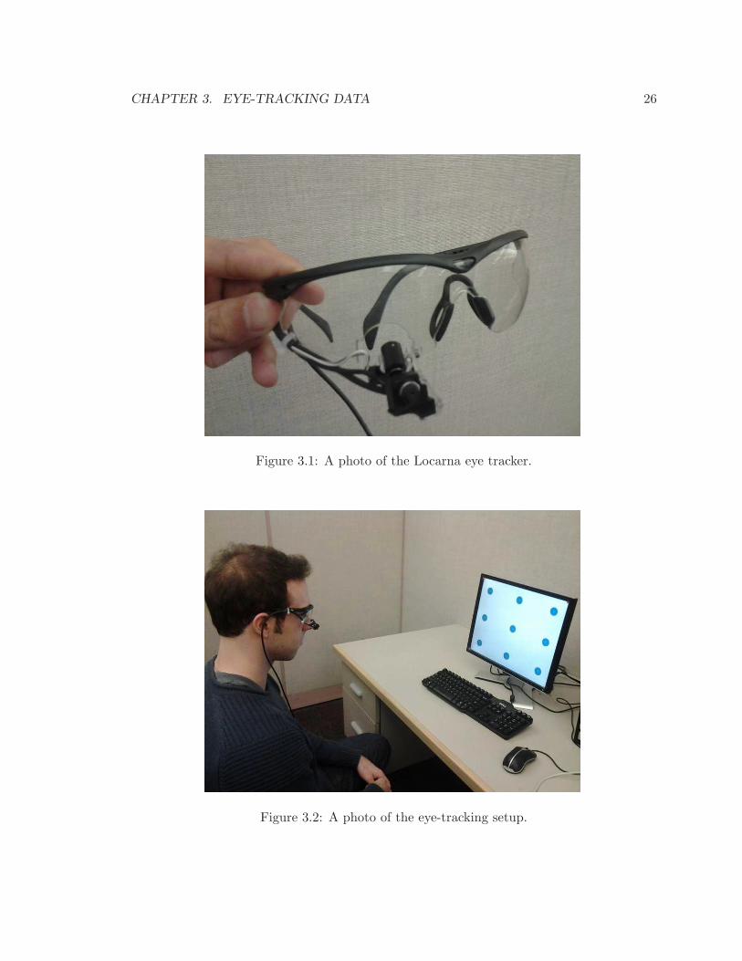
CHAPTER 3. EYE-TRACKING DATA 26
Figure 3.1: A photo of the Locarna eye tracker.
Figure 3.2: A photo of the eye-tracking setup.
CHAPTER 3. EYE-TRACKING DATA 27
the gaze locations onto the screen using a homographic transformation, without a head
tracker. Given our experimental setup, subjects did not need to move their head much and
further they remained at a fixed distance from the screen (80 cm) which allowed for a more
precise mapping of the gaze data back onto the screen plane. Fig. 3.2 shows a picture of
our experimental setup.
The advertised accuracy of the Locarna eye tracker is 1 or better in the field of view,
which is the same as the advertised accuracy of other eye trackers on the market (e.g.,
Tobii, faceLAB, etc.). To verify this, we measured the accuracy of Locarna’s eye tracker
on 10 subjects. Out of these 10 subjects, 4 persons were wearing contact lenses, and the
other 6 persons had normal vision. The subjects were graduate students in the School of
Engineering Science at Simon Fraser University.
Each subject was seated in front of a 19′′ Samsung SyncMaster 915N color monitor at
a distance of 80 cm. The monitor resolution was set to 800 × 600, with vertical frequency
of 75 Hz and horizontal frequency of 46.875 kHz. Other options were set to their factory
default values. We first displayed the nine blue calibration dots shown in Fig. 3.3 on the
monitor to calibrate the eye tracker. In the calibration procedure, the subject is instructed
to fixate on the center of each of the nine dots in sequence: dot 1, dot 2, ..., dot 9. Each
fixation was triggered by a vocal sound instructing the subject to look at the next dot.
After each fixation, the two images captured by the scene camera and the eye camera were
recorded for further processing. At the end of the calibration procedure, we obtained nine
sets of coordinates in the real-world scene (the centers of the nine blue dots), and nine pupil
locations. A manual inspection was then performed to make sure that the obtained center
locations are correct and accurate. Finally, the obtained coordinates were used to compute
the calibration matrix using a typical 8-point perspective projection and Singular Value
Decomposition (SVD).
To test the eye tracker accuracy, we asked the subjects to fixate at each of the 12 red
test dots shown in Fig. 3.4 for about one second, starting with the dot labeled “A,” then
moving to dot labeled “B” and so on up to dot labeled “L.” The radius of the dots was 32
pixels. The relative position of the red test dots with respect to the blue calibration dots is
shown in Fig. 3.5. As seen in Fig. 3.5, the test dots are positioned in between the calibration
dots. The goal of this first test was to examine the accuracy of the eye tracker immediately
after the calibration.
After the first test, we displayed a video (Stefan, CIF resolution) at the center of the

CHAPTER 3. EYE-TRACKING DATA 28
Figure 3.3: The dot pattern used for calibration.
Figure 3.4: The dot pattern used for testing.

CHAPTER 3. EYE-TRACKING DATA 29
Figure 3.5: The relative position of the test dots with respect to the calibration dots.
screen for about 7 seconds. The subjects were instructed to look wherever they wish in
the video during this time. After they were shown the video clip, the accuracy test was
repeated on the red dot pattern shown in Fig. 3.4. The subjects were again asked to look at
the test dots in sequence, starting with the dot labeled “A,” down to the dot labeled “L.”
The goal of this second test was to examine the accuracy of the eye tracker some time after
the calibration.
In order to measure the accuracy of the eye tracker, we first isolated those frames that
recorded the fixation. These were the frames where the point of gaze did not move by more
than n pixels inm consecutive frames. In other words, in a fixation group of frames, the gaze
point is allowed to move by at most n pixels in m consecutive frames. In our experiments,
we set n = 50 pixels and m = 7 frames. There were 6770 fixation frames in total, hence, on
average, 677 per subject.
We then computed the Euclidean distance between the center of each test dot and the
gaze location provided by the eye tracker in each frame of the corresponding fixation group.
The computed distances were considered as the measurement errors in estimating the gaze
location by the eye tracker. The obtained measurement errors are reported in Tables 3.1-3.3.

CHAPTER 3. EYE-TRACKING DATA 30
Table 3.1: Measurement error on all ten subjects.
Mean Standard Deviation
16.56 pixels (0.45) 13.36 pixels (0.36)
Table 3.2: Measurement error on subjects with/without contact lenses.
Subjects Mean Standard Deviation
without contact lenses 15.61 pixels (0.42) 11.25 pixels (0.30)with contact lenses 18.78 pixels (0.51) 16.86 pixels (0.45)
Difference 3.17 pixels (0.08) 5.61 pixels (0.15)
As seen in the tables, the average measured errors were under 0.5 of visual angle.
To check whether wearing contact lenses makes a difference to the accuracy, we performed
a t-test [78] on the measurement errors with and without contact lenses in Table 3.2. The
null-hypothesis was that the errors come from distributions with the same mean but unequal
variance. The two-tailed p-value in this case was 9.3543 × 10⁻⁵, indicating that the null-
hypothesis needs to be rejected, and that the errors do come from distributions with different
means. A similar test was performed for the two cases in Table 3.3 (before and after watching
the video clip). The p-value was 7.8772× 10⁻⁵ in this case, again indicating that the errors
come from distributions with different means.
Based on the obtained results, the measurement error in the case of contact lenses tends
to be higher than the error without lenses. However, the difference in the mean error in the
two cases is very small, less than 0.1. Fig. 3.6 shows two samples of the pupil detected by
Locarna’s eye tracker when using a hard contact lens. These two samples were extracted
from a 1.5 hour video recorded by Locarna’s eye tracker. As seen from these two samples,
the pupil has been detected correctly.
Table 3.3: Measurement error before and after watching the video clip.
Viewing Mean Standard Deviation
before watching the video clip 15.63 pixels (0.42) 13.24 pixels (0.35)after watching the video clip 18.25 pixels (0.49) 13.16 pixels (0.35)
Difference 2.62 pixels (0.07) 0.08 pixels (0.00)

CHAPTER 3. EYE-TRACKING DATA 31
Figure 3.6: Two samples of the pupil detected by Locarna’s eyetracker when using a hardcontact lens.
We also note that the measurement error was higher on the second test (after watching
the video clip) than on the first test, but again the difference in the mean error was very
small, less than 0.1. Overall, the mean measurement errors were around 0.5, well below
the advertised accuracy of the Locarna eye tracker of 1. Even the mean error plus one
standard deviation of the error was less than the advertised accuracy.
We uploaded a sample video of the performed experiment at the following online link
at YouTube: http://www.youtube.com/watch?v=lOL38F2VBFE. This video shows the ac-
curacy of the eye tracker on a subject wearing contact lenses with a mean error of about
0.5 of visual angle, which was roughly the mean error on the subjects with contact lenses.
The video shows the measured gaze point with a cross-hair, along with two concentric cir-
cles. The smaller circle has a diameter of 1 (i.e., radius of 0.5), and the larger circle has
a diameter of 2 (radius of 1). Overall, the tests confirmed the accuracy of the Locarna
eye-tracker. This testing represents one of the unique features of our dataset. Most other
datasets simply quote the advertised accuracy of their eye tracker, without really putting it
to test.
3.2.3 Eye-tracking data collection
A total of 15 non-expert participants (2 women and 13 men) took part in the eye-tracking
data collection study. They were recruited by a mass e-mail invitation and were paid
$15 for their participation. All of them had normal or corrected-to-normal vision, and
were asked to wear a Locarna “Pt-Mini” head mounted eye tracker [77] to determine their
gaze direction. The participants consisted of undergraduate and graduate Simon Fraser
University students aged between 18 and 30. None of the participants wore spectacles. The

CHAPTER 3. EYE-TRACKING DATA 32
pupil images captured by the eye camera were analyzed (in real time) by specific image
processing techniques implemented in the eye tracker’s software in order to find the exact
location of the pupil center.
In order to map the location of the pupil to the real-world scene (i.e., scene camera
view), a calibration matrix, obtained using the 9-dot calibration procedure described in
Section 3.2.2, was used. In order to verify that the eye tracker remained calibrated through-
out the duration of the experiment, a small crosshair was displayed on a blank screen
after presenting each video clip, and the subjects were asked to fixate on the center of the
crosshair. Any deviation from the true location was used as an out-of-calibration indicator.
This allowed us to recalibrate the system in case of any miss-calibration.
The study was performed one participant at a time over a period of two days in June
2010. The experiment was run in a quiet room with an ambient light of 200 Lux, as
recommended in [79] to simulate a “home environment.” Each participant was seated in
front of a 19′′ Samsung SyncMaster 915N color monitor at a distance of 80 cm, and watched
a video with pre-recorded instructions on how to complete the experiment before getting
started. The monitor resolution was set to 800× 600, with vertical frequency of 75 Hz and
horizontal frequency of 46.875 kHz. Other options were set to their factory default values.
The video clips were shown on the screen at twice their normal size so that they would
occupy approximately 84% of the screen. The actual size of the video frames was about 40
of the visual angle. The video resolution was increased using nearest neighbor interpolation.
This did not create visible artifacts at the viewing distance of 80 cm.
The 12 short video sequences were presented sequentially in a fixed order with a 3
second pause in-between. During this pause and before the beginning of each video, a small
crosshair (centered on the video display area) was presented and the participants were asked
to fixate on it. After the 12 videos had been presented, participants then had a 2-minute
break after which the 12 videos were presented again. The participants were asked to look
naturally at the videos and were not given any instructions as to what to look for in the
sequences.
3.2.4 Gaze data visualization
The collected raw gaze data was analyzed, mapped from the head mounted eye tracker
onto the video plane and stored in a comma separated value (CSV) file format. This file
contains the frame-by-frame, pixel wise x- and y-coordinates (measured from the bottom

CHAPTER 3. EYE-TRACKING DATA 33
left corner) of the gaze location for each participant and each of the video sequences. All
the obtained gaze data were inspected both manually and automatically to ensure that they
are fairly reliable. Each gaze location stored in the mentioned CSV files was flagged as
either correct (flag = 1) or incorrect (flag = 0) in a separate CSV mask file. The gaze data
were also represented in two different visualizations for each video sequence: a moving heat
map and a gaze plot comparing participants’ first and second viewing of the sequences. In
the heat map visualization (Fig. 3.7), the areas of the video that received the most visual
attention are presented in white, followed by red, yellow green and blue as visual attention
dropped. The heat maps were generated from the valid raw gaze location points collected
for all participants based on the characteristics of the fovea. In each frame, we create a
circular area with values following a Gaussian distribution around the gaze location of each
participant. This Gaussian models the non-uniform distribution of the photoreceptors on
the retina (i.e., the eccentricity of the fovea). The width of the Gaussian was set to 2 degrees
of visual angle, which translates to 64 pixels in our case. The accumulation of the obtained
Gaussian values resulted in the heat map for that frame. In the gaze plot visualization (Fig.
3.8), a pair of connected circles represent where each participant looked at the sequences
the first and second time they were presented to them. Each participant’s gaze location for
the first and second view is represented in a different color. This data was collected in an
effort to determine if a person who had just seen a particular video, and was thus familiar
with it, would look at the same locations when viewing it a second time.
3.2.5 Database location, structure and accessibility
The database is available online at the following URL: www.sfu.ca/~ibajic/datasets.html.
Each of the 12 video sequences is stored in a separate folder that contains the following:
• Original uncompressed sequences in YUV 4:2:0 format.
• Heat map visualization (-heatmap) video clips in compressed AVI format, similar to
Fig. 3.7.
• First and second view visualization (-1vs2) video clips in compressed AVI format,
similar to Fig. 3.8.
• A CSV file containing the x- and y-coordinates for each participant’s first and second
viewing for each frame of each video sequence.

CHAPTER 3. EYE-TRACKING DATA 34
Figure 3.7: Heat map visualization of City for the first viewing.
Figure 3.8: Gaze plot visualization comparing first and second viewing of City.

CHAPTER 3. EYE-TRACKING DATA 35
Table 3.4: Average distance between gaze locations in the first and second viewing.
Sequence Average DistancePixels % of diagonal
Bus 91.52 20.12City 72.35 15.91Crew 99.23 21.82
Foreman 46.18 10.15Flower Garden 92.74 20.39Hall Monitor 67.62 14.87
Harbor 78.27 17.21Mobile Calendar 145.95 32.09
Mother & Daughter 70.03 15.40Soccer 82.62 18.17Stefan 41.38 9.10Tempete 65.60 14.42
• A CSV file containing the binary flag matrix (-Mask) for each frame of each video
sequence.
• A number of MATLAB functions to generate and visualize the heat maps and gaze
data, as well as a user manual for the code.
• A brochure for the employed eye tracker (Pt-Mini), and a number of whitepapers and
technical papers, which are also accessible at http://www.locarna.com/docs/.
3.3 Results
3.3.1 Congruency of first vs. second viewing
It is natural to ask whether people who view a particular video multiple times look at the
same locations each time they view it. We hypothesized that this would not always be
the case. In other words, we expect that in many cases people would tend to shift their
gaze to different locations each time they view a particular video clip. We thus collected
gaze location data for two sequential viewings of each sequence in our database in order to
corroborate this hypothesis.
The gaze tracking data allowed us to compare where the participants’ gaze was directed
for each of the sequences the first time participants saw them, as well as when they were

CHAPTER 3. EYE-TRACKING DATA 36
viewed a second time. In each frame, there is a gaze location for the first and second
viewing for each participant. Visualizations of the gaze locations for the first and second
viewing (similar to Fig. 3.8) are also made available in the database. As anticipated, there
was a notable difference in the locations of the participants’ gaze for the first and second
viewing. We computed the Euclidean distance between participants’ gaze location on the
first and second viewing, and then averaged those distances across different participants.
The average distance for each of the video sequences is presented in Table 3.4, both in terms
of pixels, and in terms of the percentage of the size of the CIF frame diagonal, which is√3522 + 2882 = 454.8. As seen in the table, the average distance between the gaze locations
could be as large as a quarter of the frame. Note, however, that the variability between the
first and second viewing is likely to be influenced by the amount of time elapsed between
the two viewings. Our main goal here is to raise awareness among the readers that such
variability may exist, rather than provide an accurate model for such variability.
The shift in gaze locations was particularly evident for sequences such as Crew, Flower
Garden, and Mobile Calendar, where there are numerous objects (none of which are strongly
dominant) that compete for viewer’s attention. Here, the word “dominant” refers to our
subjective impression of what was dominant in a particular sequence or set of frames (e.g.,
the face in the initial part of Foreman). In cases where there was no single dominant object,
the viewers tended to shift their gaze to a different object in the second viewing. On the
other hand, in sequences with a single dominant object of interest, such as City and Stefan,
the differences in gaze locations were related to the size of the object - small object (the
tennis player) in Stefan gave rise to a small difference, while the large object (the central
building) in City gave rise to a large difference. Bear in mind that in these sequences, as in
those with multiple objects of interest, the gaze location did change between the first and
second viewing, but usually remained within the dominant object of interest, as illustrated
in Fig. 3.8.
Certain sequences presented interesting patterns when comparing first and second view-
ing. An example is Foreman, where the distance between gaze locations of the first and
second viewing varied as the sequence progressed (Fig. 3.9). In the beginning of the se-
quence, when there is a face present in the video, gaze was concentrated on this face in both
viewings. Hence, the gaze location difference in this part of the sequence was relatively
small. As the sequence progresses, the camera pans to show a construction site, and there
was a larger disparity between participants’ gaze locations for the first and second viewing,

CHAPTER 3. EYE-TRACKING DATA 37
Figure 3.9: Average distance (in pixels) between gaze locations in the first and secondviewing for Foreman, presented frame by frame.
because within the construction site, a larger number of regions of similar saliency compete
for viewer’s attention. In Fig. 3.9, we can see a definite trend: gaze distance between first
and second viewing increases as the sequence progresses, and peaks between frames 180-190
when the camera starts to pan to the right. In general, such a behavior depends on the
video content.
3.3.2 Accuracy of two popular visual attention models
One of the possible uses of this database is in testing prediction models of human attention.
To show how this can be done, we utilized the gaze location data to determine the accuracy
of two well-known visual attention prediction models: the Itti-Koch-Niebur (IKN) model
[2], and the Itti-Baldi (IB) model [17], [57], [58]. Using the gaze location data, we were
able to determine how well these two attention prediction models perform on each of the
sequences in the database.
For each frame, both models produce a saliency map s(x, y) that contains a predicted
attention potential value (ranging from 0 to 255) for each pixel. However, they do not
produce the same total saliency in each frame. In other words,∑s(x, y) is, in general,
different for the two models. In order to have a fair comparison between the two models,

CHAPTER 3. EYE-TRACKING DATA 38
we normalized saliency values as follows:
s′(x, y) =s(x, y)∑s(x, y)
Npixel, (3.1)
whereNpixel is the number of pixels in the frame. In our case (CIF resolution), Npixel = 352×288 = 101, 376. After this normalization, both models produce the same total normalized
saliency per frame, i.e.,∑s′(x, y) = Npixel for both models.
Using the normalized saliency maps, we proceeded to calculate the accuracy of the
models by adding the normalized values of every pixel where a gaze was directed. If (xi, yi)
is the pixel where i-th viewer’s gaze was directed in a particular frame, the accuracy score
of a model for that frame was computed as
Score =15∑
i=1
∑
(x,y)
wxi,yi(x, y)s′(x, y), (3.2)
where i goes from 1 to 15 because there were 15 viewers in our study, and wxi,yi(x, y) is a
2-D isotropic Gaussian function centered at the i-th gaze location (xi, yi),
wxi,yi(x, y) =1
2πσ2exp
(−(x− xi)
2
2σ2+
(y − yi)2
2σ2
). (3.3)
This Gaussian function models both the non-uniform distribution of the photoreceptors
on the retina, as well as the eye tracker measurement noise. It is assumed isotropic (i.e.,
σ = σx = σy) for convenience, and we set σ = 64 pixels, which corresponds to 2 degrees of
visual angle. The average accuracy scores (over all frames) for each sequence are presented
in Table 3.5, for both the first and second viewing. To examine whether the difference
in the average scores between the IKN model and the IB model is statistically significant,
we performed a paired t-test [78] on the frame-by-frame scores for each sequence and each
viewing. The null-hypothesis was that the scores of both models come from the distributions
with the same mean. Based on the results, the null-hypothesis was rejected (at the 5%
significance level) in both viewings for all sequences. The obtained p-values were less than
10−6, except for Foreman for the first viewing (p = 0.000055), and Mother & Daughter for
the first viewing (p = 0.002416) and the second viewing (p = 0.000027). Therefore, based on
our data, the difference in the average accuracy scores of two models was highly statistically
significant in each case, and the model with the higher average score on a particular sequence
can be considered more accurate on that sequence.

CHAPTER 3. EYE-TRACKING DATA 39
Table 3.5: Average accuracy score for predicting gaze location in first and second viewings.
Sequence IKN Model [2] IB Model [17]View-1 View-2 View-1 View-2
Bus 23.50 20.83 15.77 14.94City 9.12 10.67 13.39 14.61Crew 19.60 18.95 16.16 16.53
Foreman 28.99 30.01 25.15 24.50Flower Garden 51.31 48.93 19.35 20.48Hall Monitor 81.62 83.71 59.35 59.00
Harbor 31.12 36.81 20.73 23.71Mobile Calendar 44.74 40.21 21.40 21.17
Mother & Daughter 32.63 35.13 29.48 30.96Soccer 31.19 29.12 23.04 22.62Stefan 67.42 66.91 51.26 48.69Tempete 34.33 34.05 28.02 28.80
Several observations can be made from the data in Table 3.5. First, the IKN model [2]
showed better accuracy than the IB model [17] in 11 out of 12 sequences, while the IB model
was more accurate in just one case (City). This finding is somewhat surprising, given that
the IB model is more recent [17] and claimed to be an improvement over the IKN model.
We also ran the t-test to determine if there is any statistical basis for claiming that
a particular model had better accuracy on the first or second viewing. The results were
mixed. At the 5% significance level, the IKN model showed better accuracy on the first
viewing for three sequences (Bus, Mobile Calendar, and Soccer), and on the second viewing
for four sequences (City, Foreman, Harbor, and Mother & Daughter), while for the remain-
ing sequences the difference was not statistically significant. The IB model showed better
accuracy on the first viewing for three sequences (Bus, Foreman, and Stefan), and on the
second viewing for five sequences (City, Flower Garden, Harbor, Mother & Daughter, and
Tempete), while there was no statistically significant difference on other sequences. Overall,
according to this data, both models seem to be roughly equally suitable for first and second
viewing.
While Table 3.5 provides the data to compare the relative accuracy of the two models,
it is natural to ask how accurate these models are in absolute terms. One way to tackle
this question is to compare these models with uniformly spread saliency. Suppose we assign
the same saliency to each pixel, i.e., su(x, y) = 1 for all (x, y). With such uniformly spread
saliency, the total normalized saliency is the same as for the two models above (∑su(x, y) =
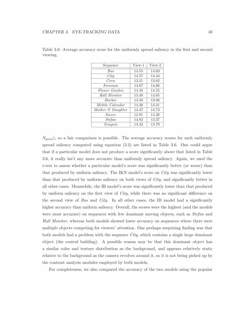
CHAPTER 3. EYE-TRACKING DATA 40
Table 3.6: Average accuracy score for the uniformly spread saliency in the first and secondviewing.
Sequence View-1 View-2
Bus 14.55 14.63City 14.57 14.44Crew 13.21 13.62
Foreman 14.67 14.66Flower Garden 14.48 14.55Hall Monitor 13.48 14.65
Harbor 14.50 13.86Mobile Calendar 14.26 14.41
Mother & Daughter 14.47 14.73Soccer 12.91 14.26Stefan 14.82 13.37Tempete 14.42 13.79
Npixel), so a fair comparison is possible. The average accuracy scores for such uniformly
spread saliency computed using equation (3.2) are listed in Table 3.6. One could argue
that if a particular model does not produce a score significantly above that listed in Table
3.6, it really isn’t any more accurate than uniformly spread saliency. Again, we used the
t-test to assess whether a particular model’s score was significantly better (or worse) than
that produced by uniform saliency. The IKN model’s score on City was significantly lower
than that produced by uniform saliency on both views of City, and significantly better in
all other cases. Meanwhile, the IB model’s score was significantly lower than that produced
by uniform saliency on the first view of City, while there was no significant difference on
the second view of Bus and City. In all other cases, the IB model had a significantly
higher accuracy than uniform saliency. Overall, the scores were the highest (and the models
were most accurate) on sequences with few dominant moving objects, such as Stefan and
Hall Monitor, whereas both models showed lower accuracy on sequences where there were
multiple objects competing for viewers’ attention. One perhaps surprising finding was that
both models had a problem with the sequence City, which contains a single large dominant
object (the central building). A possible reason may be that this dominant object has
a similar color and texture distribution as the background, and appears relatively static
relative to the background as the camera revolves around it, so it is not being picked up by
the contrast analysis modules employed by both models.
For completeness, we also compared the accuracy of the two models using the popular

CHAPTER 3. EYE-TRACKING DATA 41
receiver operating characteristic (ROC) area under curve (AUC) measure [80],[81],[82]. In
order to compute the AUC score for a saliency map, the hit rate is computed by determining
the locations where the saliency map is above a certain threshold and a fixation is present in
those regions. Similarly, the false alarm rate is computed by finding the locations where the
saliency values are above the threshold while there is no fixation present in those regions.
The ROC curve is then generated by varying the threshold to cover a wide range of possible
saliency values. The area under the ROC curve is the AUC score. An AUC value of 0.5
corresponds to pure chance, a value greater than 0.5 indicates positive correlation, and 1.0
corresponds to a perfect prediction of eye fixations [80].
The mean AUC scores of the two models for each viewing are shown in Table 3.7. To
check for the statistical difference between the mean AUC scores of the two models, we
performed a t-test with the null hypothesis that the mean AUC scores of the two models
come from Gaussian distributions with equal means. The resultant p-values are also reported
in this table. As seen from the results in this table, the IKN model outperforms the IB model
in 8 out of 12 cases on the first viewing, and in 6 out of 12 cases on the second viewing.
We also note that the performance of the two models is statistically the same on Mother
& Daughter on both viewings, since the p-value is larger than 0.05. In all other cases, the
corresponding p-values are below 0.05, which means that one of the methods obtained a
statistically significant advantage in the average score. We also observe that the accuracy
of the two models on City is around the chance level in both viewings, a result that was
previously observed in Table 3.5. Fig. 3.10 shows the average ROC curve of the two models
(across all the 12 sequences) for both viewings. As seen from these results, the average
accuracy of the IKN model is better than the IB model across all the tested sequences.
More specifically, in the first viewing, the average AUC score of the IKN model is about
0.6586 while the average AUC score of the IB model is about 0.6447 with a p-value of
0.022343. In the second viewing, the average AUC score of the IKN model is about 0.6599
while the average AUC score of the IB model is about 0.6561 with a p-value of 0.037517.
3.4 Conclusions
As video compression and processing algorithms evolve to incorporate models of human per-
ception and attention, it becomes imperative to have the tools to test them. In this chapter

CHAPTER 3. EYE-TRACKING DATA 42
Table 3.7: Average AUC score for predicting gaze location in first and second viewing.
Sequence View-1 View-2IKN IB p-value IKN IB p-value
Bus 0.621949 0.556842 0.000000 0.594323 0.526464 0.000000City 0.465959 0.518376 0.000000 0.468320 0.521248 0.000000Crew 0.589822 0.573459 0.004724 0.558933 0.577167 0.000439
Foreman 0.651316 0.615346 0.000000 0.673088 0.637185 0.000000Flower Garden 0.641450 0.572421 0.000000 0.645224 0.585146 0.000000Hall Monitor 0.818588 0.803635 0.000002 0.814053 0.798362 0.000002
Harbor 0.603295 0.552790 0.000000 0.641240 0.606229 0.000000Mobile Calendar 0.662766 0.665117 0.658195 0.675020 0.668334 0.203678
Mother & Daughter 0.662984 0.747836 0.000000 0.669394 0.772578 0.000000Soccer 0.724149 0.657288 0.000000 0.691267 0.631822 0.000000Stefan 0.786270 0.812734 0.000059 0.806129 0.839072 0.000007Tempete 0.674131 0.660761 0.002250 0.682309 0.709505 0.000000
we presented an eye-tracking database for a set of 12 standard CIF video sequences com-
monly used in the literature to compare video compression and processing algorithms. The
database itself is available for public download at www.sfu.ca/~ibajic/datasets.html.
We have described the procedure followed in order to produce this database, and also pre-
sented a preliminary analysis of the obtained data. An interesting finding stemming from the
data is that gaze locations tend to be different in different viewings of the same video, which
may have implications in the design of compression algorithms intended for one-time viewing
(e.g., videoconference), compared to those intended for multiple viewings (e.g., DVD and
Blu-ray). We also showed how the data can be used to compare models of visual attention in
terms of their accuracy in predicting gaze locations. The eye-tracking data provided in this
database can also be utilized for measuring the subjective quality of videos. For instance,
the eye-tracking heat maps of the videos can be employed as a weight map to compute an
Eye-tracking-Weighted Peak Signal to Noise Ratio (EWPSNR) [72]. Using this approach,
the PSNR values in fixation regions get a higher weight than the rest of the frame. This
makes the conventional PSNR more relevant for measuring the subjective quality of videos.
The MATLAB code for computing the EWPSNR metric is also available in the database.
It is worth pointing out that EWPSNR is similar to the Foveal Weighted SNR (FWSNR)
metric proposed in [83]. However, unlike FWSNR, EWPSNR uses the actual gaze point
measurements to weight the MSE distortion.
Some of the limitations of the database include the accuracy of the data, which is limited
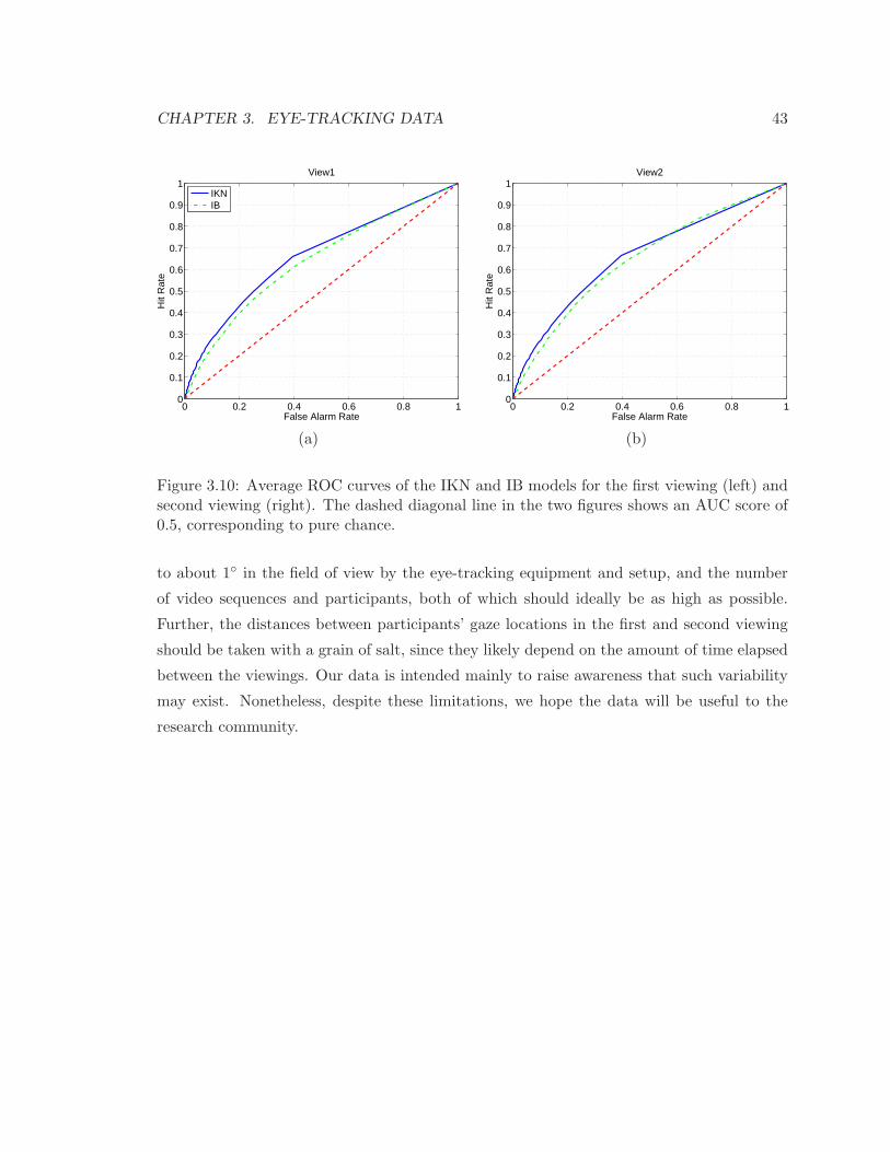
CHAPTER 3. EYE-TRACKING DATA 43
0 0.2 0.4 0.6 0.8 10
0.1
0.2
0.3
0.4
0.5
0.6
0.7
0.8
0.9
1View1
False Alarm Rate
Hit
Rat
e
IKNIB
(a)
0 0.2 0.4 0.6 0.8 10
0.1
0.2
0.3
0.4
0.5
0.6
0.7
0.8
0.9
1View2
False Alarm Rate
Hit
Rat
e
(b)
Figure 3.10: Average ROC curves of the IKN and IB models for the first viewing (left) andsecond viewing (right). The dashed diagonal line in the two figures shows an AUC score of0.5, corresponding to pure chance.
to about 1 in the field of view by the eye-tracking equipment and setup, and the number
of video sequences and participants, both of which should ideally be as high as possible.
Further, the distances between participants’ gaze locations in the first and second viewing
should be taken with a grain of salt, since they likely depend on the amount of time elapsed
between the viewings. Our data is intended mainly to raise awareness that such variability
may exist. Nonetheless, despite these limitations, we hope the data will be useful to the
research community.

Chapter 4
Computationally-Efficient Saliency
Estimation
4.1 Background
As mentioned in Chapter 2, the Itti-Koch-Niebur (IKN) saliency model [2] is one of the
most well-known and widely-used bottom-up models of visual attention. However, this
model is very complex as it requires multiresolution analysis of the input image or video in
the pixel domain in various feature channels such as intensity, color, orientation, flicker, and
motion. Hence, the high computational complexity of the IKN model limits its applications,
especially in real-time scenarios, where fast saliency estimation is required.
In this chapter, we present two computationally-efficient saliency estimation methods.
The first one is a convex approximation to the IKN model for both static images and video,
which operates solely in the Discrete Cosine Transform (DCT) domain. The computational
cost of this approximation is only a fraction of that of the IKN model, while at the same
time, its accuracy is very close to the that of the IKN model. The lower computational
cost is due to the fact that our approximation does not require multiresolution analysis as
it operates in the DCT domain in which different DCT coefficients carry the information
from different resolution levels. Many image and video processing systems (e.g., codecs)
incorporate DCT. Hence, DCT information is often available at no extra computational
cost, and it makes good engineering sense to reuse it. In addition to the lower computational
cost, the convexity of our approximation makes it attractive to incorporate within various
44
CHAPTER 4. COMPUTATIONALLY-EFFICIENT SALIENCY ESTIMATION 45
optimization procedures in image and video processing. One example is given in Chapter 6,
where this approximation is used to make a saliency-cognizant error concealment problem
convex, which in turn leads to an efficient solution.
It is worth pointing out that in [84], a saliency detection method for static images in
the JPEG compressed domain was proposed. In this method, several features such as the
intensity, color, and texture information are first extracted from the DCT coefficients of
each 8×8 block in the image. For example, the DC values of the luma and chroma channels
are converted to the RGB color space so that the intensity and color opponent features
(i.e., blue-yellow and red-green) can be computed for each block. The AC coefficients of
each block are also used to extract the orientation or texture information of each block.
This gives a texture feature vector per each 8 × 8 block. In the end, four feature maps
are created: one intensity, two color opponent features, and one texture feature. The next
step in this method is to compute the feature difference between the feature values of each
pair of blocks in each feature map. To measure the feature difference in the intensity and
color opponent channels, the feature values are directly subtracted from each other while
a Hausdorff distance [84] is used to measure the dissimilarity between two texture feature
vectors in the texture feature map. The saliency value for each DCT block in each feature
map is then determined by the block differences between each DCT block and all other
DCT blocks of the input image. The block differences are also weighted by a Gaussian
function of the Euclidean distance so that spatially-closer blocks have more contribution to
the saliency value of each block. This step gives a conspicuity map for each feature map.
The final saliency map is then computed by combining all the computed conspicuity maps
using a specific fusion method [84].
Although the method from [84] works in the DCT domain, it is different from our pro-
posed approximation to the IKN model in several aspects. First, unlike [84], our method
attempts to approximate the well-known IKN saliency, rather than provide a saliency es-
timate based on some other principles. Second, our method offers an estimate of saliency
that is convex in the input data, which makes it attractive for use in various optimization
problems. Third, the computational complexity of our method appears to be lower than
that of [84], since our method simply sums up the weighted squared magnitudes of the DCT
coefficients of individual image blocks, whereas the method in [84] involves computing and
combining several feature maps over the entire image.
The second saliency estimation method presented in this chapter is an extension of the
CHAPTER 4. COMPUTATIONALLY-EFFICIENT SALIENCY ESTIMATION 46
abovementioned convex approximation to IKN saliency. The main difference is in the part
that estimates motion-induced saliency, where we incorporate global motion compensation
(GMC) [14] prior to saliency estimation. Although this second method is not convex in
the input data and is more complex than the first method, it is still simpler than the IKN
saliency model and offers comparable accuracy, somewhat higher on sequences with camera
motion.
This chapter is organized as follows. In Section 4.2, we present our convex approximation
to the IKN saliency model. We then present the second saliency estimation method based
on GMC in Section 4.3. The results are presented in Section 4.4. We provide an analysis
of the computational complexity of the proposed saliency detection methods in Section 4.5,
and conclusions are drawn in Section 4.6.
4.2 A convex approximation to IKN saliency
Our convex approximation to the IKN saliency consists of two parts: spatial and temporal.
Let X be a block within a given frame. We will show how to compute an approximation
S(X) to the IKN saliency of that block.
The dyadic Gaussian pyramid employed in the IKN model approximately halves the
normalized frequency spectrum of the input image at each level due to the successive low-
pass filtering. Since the normalized frequency (in radians/pixel) of the original image at level
0 is [0, π] in both horizontal and vertical directions, the normalized frequency spectrum at
level c of the pyramid is in the range [0, π/2c]. Hence, the normalized frequency spectrum
at levels 4 and 8 will be, respectively, in the range [0, π/16] and [0, π/256]. As mentioned in
Section 2.2.1, in the IKN model, a center-surround feature map at center level c ∈ 2, 3, 4and surround level s = c+δ, with δ ∈ 3, 4, is computed by interpolating the surround level
to the center level followed by point-by-point subtraction. Hence, the normalized frequency
spectrum of the center-surround feature map at center level c and surround level s will be,
in the range [π/2s, π/2c]. To compute the conspicuity map of each feature channel, all the
computed center-surround feature maps are resized to the size of level 4. Hence, the upper
limit of the normalized frequency spectrum of the obtained conspicuity map is capped by
π/16. Since the smallest surround map is at level 8, we conclude that the IKN model uses
the image content in the normalized frequency range [π/256, π/16] to construct the saliency
map, as already observed in [1, 85]. Note that the normalized frequency (in radians/pixel)
CHAPTER 4. COMPUTATIONALLY-EFFICIENT SALIENCY ESTIMATION 47
is defined with respect to the original image, regardless of the resolution.
To compute spatial saliency, we need a way to use the pixels of a given block X to
estimate the saliency of the original image at that position. Based on the discussion above,
it seems natural to try to recapture the portion of the image signal from the normalized
frequency range [π/256, π/16] at the position of the block X. However, the process of
extracting a block from an image involves windowing and spectral down-sampling, which
leads to spectral leakage. Some energy from the normalized frequency range [π/256, π/16]
of the original image will be present at other frequencies when one examines the spectrum
of the block X.
To demonstrate the effect of spectral leakage, consider a simple 1-D example shown in
Fig. 4.1. The red signal in this figure shows the 1-D DCT of a pure first harmonic signal of
length 16, which is defined as follows
x[n] = cos(2πn
16), (4.1)
for n = 0, 1, · · · , 15. We will extract a segment of length 8 from the middle part of this
signal as follows. We first multiply the signal by a rectangular window of length 8, centered
in the middle of the signal; the 1-D DCT at this point is shown as green in the figure.
Then we remove the zeros outside the interval where the window function is equal to one;
the 1-D DCT of the resulting signal is shown as blue. Note that the signal energy, which
was originally concentrated in only one DCT coefficient, has now leaked into certain higher
frequency coefficients (coefficients 3, 5 and 7). However, since the ratio of the length of the
original signal and the length of the extracted segment is an integer (16/8 = 2), no energy
has leaked into the DC coefficient (coefficient 0).
Fig. 4.2 shows another example in which the original signal length is 16 but the extracted
segment length is 7. Here, due to the non-integer ratio between the original signal length
and the extracted segment length, some energy leaks into the DC coefficient as well. Hence,
depending on the ratio between the signal size and the block size, original signal energy may
or may not leak into certain DCT coefficients.
In order to address this issue we take the following approach. Consider the original
image spectrum in the normalized frequency range [0, π]. We think of the image signal in
the normalized frequency range [π/256, π/16] as the “signal,” and the signal in the remain-
ing part of the spectrum, [0, π/256) ∪ (π/16, π], as “noise,” or “undesired signal.” After
extracting a block from the image, both the signal and the noise leak from their native

CHAPTER 4. COMPUTATIONALLY-EFFICIENT SALIENCY ESTIMATION 48
DCT Index
DC
T M
agni
tude
Original signal DCTDCT after windowingDCT of the block
Figure 4.1: A simple example showing the effect of spectral leakage. In this example, theoriginal signal is of length 16 while the extracted block is of length 8.
DCT Index
DC
T M
agni
tude
Original signal DCTDCT after windowingDCT of the block
Figure 4.2: A simple example showing the effect of spectral leakage. In this example, theoriginal signal is of length 16 while the extracted block is of length 7.

CHAPTER 4. COMPUTATIONALLY-EFFICIENT SALIENCY ESTIMATION 49
frequency bands into other bands. The spectrum of the block X is the sum of the leaked
spectra of the signal and the noise. We need to extract the signal from noise. Since the
signal and the noise come from non-overlapping frequency bands in the original image, they
are orthogonal. The Wiener filter is the optimum linear filter for extracting the signal from
noise, and when the signal and noise are orthogonal, its transfer function is [86]
H(ω) =SS(ω)
SS(ω) + SV (ω), (4.2)
where SS(ω) is the power spectral density of the signal, and SV (ω) is the power spectral
density of the noise. Hence, the Wiener filter is a frequency-domain weighting function [87].
We performWiener filtering in the DCT domain, rather than DFT domain, because DCT
is simpler to compute (no need for complex arithmetic) and its efficient implementations are
readily available in various image and video codecs. Let ZX(j, l) be the (j, l)-th 2-D DCT
coefficient of X, which is computed as follows
ZX(j, l) =1
4CjCl
Nb−1∑
y=0
Nb−1∑
x=0
X(y, x) cos
(jπ
2y + 1
2Nb
)cos
(iπ
2x+ 1
2Nb
), (4.3)
where Nb is the width (and height) of X, X(y, x) is the (y, x)-th element of X, and
Cu =
1√2
if u = 0
1 else,(4.4)
with u ∈ j, l. The Wiener-filtered coefficient is
ZWX (j, l) = H(j, l)ZX(j, l), (4.5)
where H(j, l) is a coefficient that should be computed as in (4.2) based on signal and noise
powers at the (j, l)-th 2-D DCT coefficient. A common way to design a Wiener filter is
to postulate certain signal and noise models, and derive the filter from the resulting power
spectral densities [88]. We use the 1/f -model, which is thought to be an excellent model
for natural images [89], as a starting point; our “signal” is the part of the 1/f signal in the
frequency band [π/256, π/16], and our “noise” is the part of the 1/f signal in the remainder
of the spectrum.
To compute H(j, l), we proceed as follows. We generate a deterministic 1/f 2-D signal
that covers the frequency band [π/256, π/16], at a size equal to the target image resolution.

CHAPTER 4. COMPUTATIONALLY-EFFICIENT SALIENCY ESTIMATION 50
0
2
4
6
8
10
12
14
16
0
5
10
15
20
0
0.2
0.4
0.6
0.8
l
Resolution = 352x288
j
H(j,
l)
(a)
0
2
4
6
8
10
12
14
16
0
5
10
15
20
0
0.2
0.4
0.6
0.8
l
Resolution = 1024x768
j
H(j,
l)
(b)
Figure 4.3: Wiener coefficients for a 16× 16 block for two common resolutions.
We then extract from this signal a block whose size is equal to the block size of interest and
perform a 2-D DCT on it. Let us denote the resulting DCT by ZS(i, j). Then ZS2(i, j)
is the signal power associated with that DCT coefficient, corresponding to SS(ω) in (4.2).
Similarly, we find the noise power associated with DCT coefficient (i, j), ZV2(i, j) by using
a deterministic 1/f 2-D signal that covers the frequency band [0, π/256) ∪ (π/16, π]. The
DCT-domain Wiener filter coefficients are then given by
H(j, l) =ZS
2(j, l)
ZS2(j, l) + ZV
2(j, l), (4.6)
Note that H(j, l) depends on image resolution and the block size, due to the way ZS(i, j)
and ZV(i, j) are computed, but can be easily pre-computed for typical resolutions and
block sizes. Fig. 4.3 shows the Wiener coefficients obtained by the proposed method for
two standard resolutions, 352 × 288 and 1024 × 768, and a block size of 16 × 16. Observe
that Wiener coefficients for low frequencies are larger than those for high frequencies, as one
would expect for a signal that came from the normalized frequency band [π/256, π/16] in the
original image. However, due to spectral leakage, some of the higher frequency coefficients
also contain part of the signal, which makes their Wiener coefficients non-zero.
Our approximation to the spatial saliency of block X is the power of the Wiener-filtered
CHAPTER 4. COMPUTATIONALLY-EFFICIENT SALIENCY ESTIMATION 51
signal ZWX , that is
Sspatial(X) =∑
(j,l)
(ZWX (j, l))2 =
∑
(j,l)
H2(j, l)ZX2(j, l). (4.7)
If block X has multiple color channels (e.g., YUV), the power in all channels is added
together. Since DCT is a linear operation, as is Wiener filtering, while squaring is a convex
operation, the saliency estimate Sspatial(X) in (4.7) is convex in X.
As mentioned in the review of the IKN model in Section 2.2.1, the same center-surround
mechanism that is used for the intensity, color, and orientation channels is used for comput-
ing the motion and flicker conspicuity maps. However, in the flicker and motion channels,
the center-surround mechanism is applied on the absolute luminance difference or spatially-
shifted difference between the current frame and the previous frame. Based on this fact, we
now provide a convex approximation to temporal saliency. Let X0 be the co-located block
of X in the previous frame, and let Q = |X−X0| be the residual block obtained by taking
the absolute difference between X and X0. Our approximation to the temporal saliency of
block X is the power of the Wiener-filtered signal ZWQ , that is
Stemporal(X) =∑
(j,l)
(ZWQ (j, l))2 =
∑
(j,l)
H2(j, l)ZQ2(j, l), (4.8)
where ZQ2(j, l) is the (j, l)-th 2-D DCT coefficient of Q. Note that Stemporal(X) is convex
in X because Q is convex in X, DCT and Wiener filtering are linear, and squaring is a
convex operation.
In order to get the final saliency estimate of X, we combine the spatial and temporal
saliency terms as follows
S(X) = Sspatial(X) + αStemporal(X), (4.9)
where α is a positive parameter that trades off between the two saliency terms. We note
that S(X) is convex in X because it is a non-negative linear combination of convex terms.
This saliency estimate will be evaluated and compared against the IKN saliency in
Section 4.4.1, where the results will show that (4.9) offers a very good approximation to
IKN saliency. Next, we present the second saliency estimation method, which makes use
of the spatial saliency term from above, but uses global motion compensation prior to
computing motion saliency.
CHAPTER 4. COMPUTATIONALLY-EFFICIENT SALIENCY ESTIMATION 52
4.3 Global motion-compensated saliency
It is well-known that object motion is one of the strongest attractors of visual attention [90],
[91], [55]. In many existing computational models of visual attention, such as the IKN model,
the temporal saliency is estimated by measuring the local motion contrast [67]. An object
with significant motion with respect to its surroundings would be considered as a strong,
attention-grabbing “surprise” to the visual system, and hence salient.
In [92], it was observed that the accuracy of the IKN model degrades on scenes with
camera motion. When the camera moves, the resulting apparent motion of the background
competes with foreground object motion and may confuse the saliency model, leading to
lower accuracy. To mitigate this problem, similar to [55] and [91], we remove the camera
motion prior to computing temporal saliency.
To make the process computationally efficient, particularly for video compression ap-
plications, we use the previous frame’s motion field (which is already computed) as an
approximation to the current frame’s motion field, and run an efficient global motion es-
timation algorithm [14] that uses only motion vectors (MVs), followed by global motion
compensation, i.e. subtraction of global motion from the motion field. This way, we obtain
one global motion-compensated MV (GMC-MV) per 4 × 4 block. For each block X, the
average magnitude of all GMC-MVs in it is taken as its motion saliency Smotion(X).
In order to obtain the overall global motion-compensated saliency Sgmc(X), we combine
the spatial saliency Sspatial(X) from the previous section with the abovementioned motion
saliency using the fusion method from [93], [94], as follows
Sgmc(X) = (1− αg)Sspatial(X) + αgSmotion(X) + βgSspatial(X)Smotion(X), (4.10)
where αg and βg are positive constants. The first two terms in (4.10) allow the spatial
and motion saliency to promote a block independently. On the other hand, the third term
in (4.10) weighs the spatial saliency value by the motion saliency value and vice versa.
Hence, it is a mutual reinforcement term, which promotes those blocks that are salient both
spatially and temporally. As mentioned earlier, it is known that motion cues are one of the
strongest attractors of visual attention [90]. Hence, in practice, a larger relative weight for
the motion saliency (αg > 0.5) is recommended. In our experiments, we set αg = 0.9 and
βg = 1.
Our experimental results in Section 4.4.2 indicate that the performance of the global
CHAPTER 4. COMPUTATIONALLY-EFFICIENT SALIENCY ESTIMATION 53
motion-compensated saliency estimate in (4.10) is comparable to the IKN saliency model
for video, even better when camera motion is present in the scene.
4.4 Accuracy
In this section, we first evaluate the accuracy of our convex approximation to IKN saliency in
Section 4.4.1, followed by performance evaluation of the global motion-compensated saliency
estimation method in Section 4.4.2.
4.4.1 Assessment of the convex approximation to IKN saliency
As explained in Section 4.2, our approximation to IKN saliency has two terms: spatial
and temporal. The approximation accuracy of the spatial term (4.7) with block size was
16 × 16 is assessed first on two popular still image datasets with associated ground truth
eye-tracking data (fixation points). The first dataset is the so-called Toronto data set [68],
which contains 120 RGB images (688× 512 pixels) of outdoor and indoor scenes with eye-
tracking data of 20 subjects. The second data set is the so-called MIT data set [69],[82],
which contains 1003 RGB indoor and outdoor images (1024× 768 pixels) with eye-tracking
data of 15 subjects.
The accuracy of spatial saliency detection is measured by the popular receiver operating
characteristic (ROC) area under curve (AUC) measure [80],[81],[82]. In order to compute the
AUC score for a saliency map, the hit rate is computed by determining the locations where
the saliency map is above a threshold and a fixation is present in those regions. Similarly,
the false alarm rate is computed by finding the locations where the saliency values are above
the threshold while there is no fixation present in those regions. The ROC curve is then
generated by varying the threshold to cover a wide range of possible saliency values. The
area under the ROC curve is the AUC score. An AUC value of 0.5 corresponds to pure
chance, a value greater than 0.5 indicates positive correlation, and 1.0 corresponds to a
perfect prediction of eye fixations [80].
Table 4.1 shows the average AUC scores of the spatial IKN model and our approximation
on each of the two datasets. As seen from the table, the average AUC scores of the proposed
approximation are very close to the average AUC scores of the IKN model in each of the
two datasets, indicating good approximation. To check for the statistical significance of this
observation, we performed a paired t-test [95] between the AUC scores on each pair of images

CHAPTER 4. COMPUTATIONALLY-EFFICIENT SALIENCY ESTIMATION 54
Table 4.1: Average AUC scores of the spatial IKN saliency and the proposed approximationon two common datasets.
Dataset IKN Saliency Model Proposed Approximation p-valueToronto 0.6512 0.6468 0.6233MIT 0.6261 0.6244 0.6426
in the two datasets, with the null hypothesis that the two samples come from Gaussian
distributions with equal means and unknown variances. The resultant p-values [95] are also
reported in Table 4.1. In experimental sciences, as a rule of thumb, the null hypothesis
is rejected when p < 0.05. As seen from Table 4.1, the p-value for both data sets is well
above 0.05, which indicates that the two sets of AUC scores are statistically very similar,
i.e., virtually indistinguishable.
To further compare the saliency maps produced by the proposed spatial approximation
(4.7) with those produced by the original IKN model, we employed the Kullback-Leibler
Divergence (KLD) [62]. For this purpose, we first normalized each saliency map so that it
sums up to 1, and then considered the normalized map as a 2-D probability distribution.
We then computed the average symmetric KLD between the two sets of normalized maps
on both datasets. The symmetric KLD between two probability density functions p1(x) and
p2(x) is defined as
KLDsym(p1(x)||p2(x)) =1
2(KLD(p1(x)||p2(x)) +KLD(p2(x)||p1(x))), (4.11)
where KLD(p1(x)||p2(x)) is the KLD between p1(x) and p2(x).
The average symmetric KLD on the Toronto data set was 0.01630, and it was 0.01355 on
the MIT data set. Averaging these two, taking into account the number of images in each,
the overall average symmetric KLD between the IKN saliency maps and our approximation
was 0.0138.
In order to get a feeling for what symmetric KLD of 0.0138 between saliency maps
means, we performed an experiment using JPEG coding and compared IKN saliency maps
of the original and encoded images. For this purpose, we compressed the images in the two
datasets with a JPEG encoder at various quality factors, and for each quality factor, we
computed the average symmetric KLD between the normalized IKN saliency maps of the
original images and the normalized IKN saliency maps of the compressed images. We also
computed the average PSNR for each quality factor. We then repeated this experiment

CHAPTER 4. COMPUTATIONALLY-EFFICIENT SALIENCY ESTIMATION 55
until we got an average symmetric KLD of 0.0138. At this KLD, the average PSNR was
about 40.2 dB. Therefore, one can say that the loss in accuracy in our approximation for
spatial IKN saliency is comparable to that incurred in high-quality image compression that
results in a PSNR of about 40.2 dB. Fig. 4.4 shows several sample images from the Toronto
data set, their IKN saliency maps, as well as the saliency maps generated by the proposed
spatial saliency approximation.
As a further illustration, we repeated the above experiment with a “naive” spatial
saliency approximation that uses only five DCT coefficients
(j, l) ∈ (0, 1), (0, 2), (1, 1), (1, 0), (2, 0)
and sets their weight to 1 in (4.7), while setting the weight of other coefficients to zero. These
coefficients correspond to the normalized frequency band [π/256, π/16] of a 16 × 16 block.
As shown in Fig. 4.3, these coefficients do end up with some of the highest Wiener weights,
but this approach ignores spectral leakage, which is why we call it “naive.” This “naive”
method produces saliency maps with an average KLD of 0.0165 with respect to IKN maps,
over the two datasets. Using the JPEG coding analogy above, the average KLD of 0.0165
corresponds to compression at 38.5 dB. Hence, although not as good as the Wiener-based
approach, this “naive” method still performs reasonably well in terms of spatial saliency
approximation.
We next assess the temporal saliency approximation together with spatial saliency ap-
proximation in the context of saliency estimation in video. Our complete approximation
(the combination of temporal and spatial approximation) will henceforth be referred to as
“IKN-A.” In this test, the benchmark is the IKN model outfitted by a flicker and motion
channel [67]. Table 4.2 compares the spatial IKN saliency against the approximation in
(4.7), the temporal IKN saliency against the approximation in (4.8), as well as the full
IKN saliency (with MaxNorm normalization [2], which we call it “IKN-MA” in the rest of
our analysis) against the combined saliency approximation in (4.9) on ten standard CIF
sequences at 30 frames per second (fps). As seen in the table, the average symmetric KLD
between the spatial IKN saliency and our approximation is 0.0233, which corresponds to
a PSNR of about 36.2 dB using the JPEG coding analogy above. The average symmetric
KLD between the full saliency maps is 0.0174, corresponding to a PSNR of about 38.3 dB,
which is thought to be a fairly decent quality.
Next, we compared the accuracy of IKN-A against IKN-MA using the AUC scores on

CHAPTER 4. COMPUTATIONALLY-EFFICIENT SALIENCY ESTIMATION 56
Figure 4.4: Sample images from the Toronto data set (left) along with their IKN saliencymap (middle) and the saliency map generated by the proposed approximation (right).

CHAPTER 4. COMPUTATIONALLY-EFFICIENT SALIENCY ESTIMATION 57
the the video sequences from our dataset. The results for both viewings are shown in Table
4.3. As seen from these results, the average AUC scores of IKN-A are close to those of
IKN-MA on both viewings. To check for the statistical significance, we performed a paired
t-test between the AUC scores of the two models, with the null hypothesis that the AUC
scores of the two models come from Gaussian distributions with equal means. The resulting
p-values are also reported in Table 4.3. As seen from this table, for the first viewing, in 6
cases out of 12 cases, the p-values are larger than 0.05, indicating a statistical tie. In other
cases, the accuracy of IKN-A is slightly lower than IKN-MA. The same situation holds for
the second viewing as well. Fig. 4.5 shows the average ROC curves (across all videos) of
the two models for both viewings. For the first viewing, the average AUC score of IKN-MA
across all videos is about 0.6568 while the average AUC score of IKN-A is 0.6463. For the
second viewing, the average AUC score of IKN-MA across all videos is about 0.6621 while
that of IKN-A is 0.6504.
Finally, in addition to the KLD and AUC metrics, we also compared the saliency maps
produced by IKN-MA with the saliency maps produced by IKN-A based on the average
Mean Square Error (MSE). For this purpose, all saliency maps were normalized between 0
and 255, and the average MSE value across all videos was computed. The average MSE
was about 51.53 on the sequences mentioned in Table 4.2, which is equivalent to a PSNR
of about 31 dB.
According to the results reported in this section, we conclude that the accuracy of our
proposed convex approximation to IKN saliency is satisfactory.
4.4.2 Evaluating GMC saliency estimation
In order to evaluate the performance of the global motion-compensated saliency estimation
(GMC-S) from Section 4.3, we compared it against the spatio-temporal IKN model [67]
on the eye-tracking dataset from Chapter 3. To generate the results for the IKN model,
the original implementation of the IKN model [96] was utilized. Note that, as discussed
in [67], in the original implementation of the IKN model for video, two main normalization
operators are available for combining the conspicuity and feature maps: MaxNorm and
FancyOne. MaxNorm yields smoother, more continuous saliency maps, while FancyOne
yields increasingly sparser saliency maps, with only a few sharp peaks [67]. Since the saliency
maps produced by MaxNorm are smoother than those of FancyOne, the MaxNorm operator
is thought to be better suited to video compression [67]. However, FancyOne operator is

CHAPTER 4. COMPUTATIONALLY-EFFICIENT SALIENCY ESTIMATION 58
Table 4.2: Average symmetric KLD between the IKN saliency and our approximation on12 standard CIF sequences.
Sequence Spatial Saliency Temporal Saliency Full Saliency
Bus 0.0163 0.0198 0.0147City 0.0144 0.0101 0.0115Crew 0.0107 0.0095 0.0087
Foreman 0.0304 0.0110 0.0189Flower Garden 0.0138 0.0192 0.0117Hall Monitor 0.0293 0.0102 0.0189
Mother & Daughter 0.0142 0.0101 0.0120Harbour 0.0389 0.0103 0.0243
Mobile Calendar 0.0184 0.0151 0.0146Soccer 0.0162 0.0046 0.0106Stefan 0.0477 0.0201 0.0301Tempete 0.0294 0.0315 0.0333
Average 0.0233 0.0143 0.0174
Table 4.3: Average AUC score of IKN-MA and the proposed IKN approximation (IKN-A)on twelve standard video sequences.
Sequence View-1 View-2IKN-MA IKN-A p-value IKN-MA IKN-A p-value
Bus 0.677901 0.749948 0.000000 0.642090 0.691229 0.000000City 0.586142 0.570721 0.065121 0.587870 0.564346 0.128152Crew 0.651511 0.658493 0.153853 0.655754 0.683478 0.000000
Foreman 0.642199 0.629129 0.071223 0.654281 0.646405 0.054212Flower Garden 0.644158 0.628359 0.000000 0.676063 0.624593 0.000000Hall Monitor 0.804911 0.763408 0.000000 0.816323 0.773894 0.000000
Harbor 0.537696 0.529202 0.082716 0.570529 0.566871 0.192315Mobile Calendar 0.595226 0.599049 0.497824 0.599554 0.580717 0.238125
Mother & Daughter 0.660234 0.639038 0.000005 0.631714 0.628824 0.000000Soccer 0.717283 0.684119 0.000000 0.707318 0.674214 0.000000Stefan 0.716098 0.670241 0.000002 0.752651 0.716653 0.000000Tempete 0.648412 0.633374 0.056646 0.650889 0.633327 0.338122
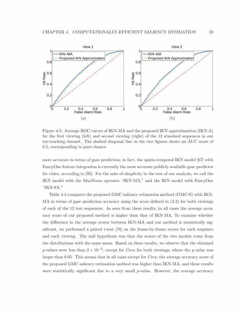
CHAPTER 4. COMPUTATIONALLY-EFFICIENT SALIENCY ESTIMATION 59
0 0.2 0.4 0.6 0.8 10
0.2
0.4
0.6
0.8
1View 1
False Alarm Rate
Hit
Rat
e
IKN−MAProposed IKN Approximation
(a)
0 0.2 0.4 0.6 0.8 10
0.2
0.4
0.6
0.8
1View 2
False Alarm Rate
Hit
Rat
e
IKN−MAProposed IKN Approximation
(b)
Figure 4.5: Average ROC curves of IKN-MA and the proposed IKN approximation (IKN-A)for the first viewing (left) and second viewing (right) of the 12 standard sequences in oureye-tracking dataset. The dashed diagonal line in the two figures shows an AUC score of0.5, corresponding to pure chance.
more accurate in terms of gaze prediction; in fact, the spatio-temporal IKN model [67] with
FancyOne feature integration is currently the most accurate publicly available gaze predictor
for video, according to [92]. For the sake of simplicity in the rest of our analysis, we call the
IKN model with the MaxNorm operator “IKN-MA,” and the IKN model with FancyOne
“IKN-FA.”
Table 4.4 compares the proposed GMC saliency estimation method (GMC-S) with IKN-
MA in terms of gaze prediction accuracy using the score defined in (3.2) for both viewings
of each of the 12 test sequences. As seen from these results, in all cases the average accu-
racy score of our proposed method is higher than that of IKN-MA. To examine whether
the difference in the average scores between IKN-MA and our method is statistically sig-
nificant, we performed a paired t-test [78] on the frame-by-frame scores for each sequence
and each viewing. The null hypothesis was that the scores of the two models come from
the distributions with the same mean. Based on these results, we observe that the obtained
p-values were less than 2× 10⁻³, except for Crew for both viewings, where the p-value was
larger than 0.05. This means that in all cases except for Crew, the average accuracy score of
the proposed GMC saliency estimation method was higher than IKN-MA, and these results
were statistically significant due to a very small p-value. However, the average accuracy

CHAPTER 4. COMPUTATIONALLY-EFFICIENT SALIENCY ESTIMATION 60
Table 4.4: Comparing the proposed GMC saliency estimation method (GMC-S) with IKN-MA.
Video First Viewing Second Viewing
IKN-MA GMC-S p-value Difference IKN-MA GMC-S p-value DifferenceBus 19.18 22.30 0.000006 +3.12 19.35 21.81 0.002081 +2.46City 15.86 33.05 0.000000 +17.19 16.04 33.77 0.000000 +17.73Crew 15.66 15.87 0.323377 +0.21 15.93 15.98 0.775784 +0.05
Foreman 20.05 22.71 0.000405 +2.66 19.99 23.67 0.000003 +3.68Flower Garden 20.69 22.07 0.000000 +1.38 21.48 23.03 0.000000 +1.55Hall Monitor 30.47 34.12 0.000245 +3.65 32.18 38.92 0.000000 +6.74
Harbor 18.83 21.27 0.001148 +2.44 19.37 22.06 0.000065 +2.69Mobile Calendar 19.42 26.09 0.000000 +6.67 19.43 28.06 0.000000 +8.63
Mother & Daughter 15.51 16.78 0.000000 +1.27 16.03 17.06 0.000000 +1.03Soccer 18.81 21.62 0.000000 +2.81 20.20 24.73 0.000000 +4.53Stefan 21.07 23.97 0.007764 +2.90 18.67 23.05 0.000189 +4.38Tempete 17.96 21.42 0.000000 +3.46 17.36 20.54 0.000000 +3.18
of the two models was statistically indistinguishable on Crew, at the 5% confidence level.
Based on this data, we can claim that the proposed GMC saliency estimation method is
more accurate than IKN-MA in terms of gaze prediction.
In order to compare the accuracy of our proposed GMC saliency estimation method with
IKN-FA, we utilized the FancyOne normalization operator on all saliency maps produced by
our GMC saliency estimation method. In other words, the saliency of each 16×16 block was
first computed as in (4.10), and then similar to the IKN model, the FancyOne operator was
applied on the resultant saliency maps to generate the final saliency maps for our method.
We then performed the same analysis as in Table 4.4 based on the obtained saliency maps.
The results are reported in Table 4.5. In this table, p-values larger than 0.05 have been
indicated in bold typeset.
According to the results in Table 4.5, we observe that the performance of the proposed
GMC saliency estimation method is statistically the same (at the 5% confidence level) as
IKN-FA on Bus (for both viewings), Crew (for both viewings), Flower Garden (for the
second viewing), Harbor (for both viewings), Stefan (for both viewings), and Tempete (for
the second viewing). In these cases, the null hypothesis cannot be rejected because the
corresponding p-values are larger than 0.05. In all other cases, the proposed GMC saliency
estimation method outperforms IKN-FA except for the first viewing of Flower Garden, and
both viewings of Hall Monitor, Mobile Calendar, and Mother & Daughter. Hence, one
could argue that the proposed GMC saliency estimation method has comparable accuracy
to IKN-FA in terms of gaze prediction.

CHAPTER 4. COMPUTATIONALLY-EFFICIENT SALIENCY ESTIMATION 61
Table 4.5: Comparing the proposed GMC saliency estimation method (GMC-S) with IKN-FA.
Video First Viewing Second Viewing
IKN-FA GMC-S p-value Difference IKN-FA GMC-S p-value DifferenceBus 23.50 21.33 0.161670 −2.17 20.83 19.23 0.365476 −1.6City 9.12 68.04 0.000000 +58.92 10.67 62.47 0.000000 +51.08Crew 19.60 20.17 0.598369 +0.57 18.95 18.83 0.891117 −0.12
Foreman 28.99 38.40 0.000000 +9.41 30.01 41.62 0.000000 +11.61Flower Garden 51.31 44.71 0.000000 −6.60 48.93 47.60 0.371274 −1.33Hall Monitor 81.62 47.31 0.000000 −34.31 83.71 55.79 0.000000 −27.92
Harbor 31.12 33.14 0.279229 +2.02 36.81 34.29 0.093973 −2.52Mobile Calendar 44.74 31.55 0.000000 −13.19 40.21 34.46 0.000708 −5.75
Mother & Daughter 32.63 18.60 0.000000 −14.03 35.13 17.84 0.000000 −17.29Soccer 31.19 39.68 0.000000 +8.49 29.12 40.15 0.000000 +11.03Stefan 67.42 73.92 0.231836 +6.50 66.91 73.50 0.242396 +6.59Tempete 34.33 37.18 0.040270 +2.85 34.05 31.70 0.086432 −2.735
The study in [92] has evaluated nine publicly available saliency models on the dataset
described in Chapter 3, which allows us to use the results from [92] in order to see how our
GMC saliency estimation method (GMC-S) and our proposed IKN approximation (IKN-
A) compare against these other models. Besides IKN-FA, the study in [92] included the
following saliency models: Schauerte and Stiefelhagen [97], Harel et al. [38], Achanta and
Susstrunk [85], Itti and Baldi [17], Goferman et al. [98], Fang et al. [99], Seo and Milan-
far [100], and Kim et al. [101], For brevity, these models will henceforth be referred to as
QDCT, GBVS, MSSS, IB, CA, QFTA, SR, WK, respectively.
The methodology employed in [92] was as follows. First, each model was applied to each
of the sequences in the dataset, resulting in one saliency map per frame for each model. Then
the score (3.2) was computed for each model in each frame using the gaze location data. The
scores were analyzed using a multiple comparisons procedure known as the Tukey-Kramer
test [102]. Specifically, for each sequence, the 95% confidence intervals for the mean score of
each model was found. The top performing models were identified as those whose confidence
intervals overlap that of model with the top mean score. Hence, for any sequence, there
could be multiple models that are considered top performers.
The resulting mean scores are shown in Tables 4.6 and 4.7 for the first viewing and
second viewing, respectively. The entries shown in bold indicate top performing models for
each sequence. The ranking in terms of the number of appearances among top performers
across both viewings is shown in Fig. 4.6. As seen from these results, out of 24 cases for the
two viewings, both GMC-S and IKN-FA appeared 12 times among top performers. Also,

CHAPTER 4. COMPUTATIONALLY-EFFICIENT SALIENCY ESTIMATION 62
Table 4.6: Mean accuracy scores for several saliency estimation methods based on the firstviewing in the eye-tracking dataset, with top scores indicated in bold.
Video IKN-FA QDCT GBVS MSSS IB CA QFTA SR WK GMC-S IKN-ABus 23.50 22.35 23.20 15.54 15.77 24.02 19.32 16.44 25.21 21.33 44.21City 9.12 15.17 23.49 15.58 13.39 18.15 18.70 10.19 10.57 68.04 16.01Crew 19.60 20.88 23.16 19.40 16.16 21.20 19.04 13.06 21.63 20.17 29.43
Foreman 28.99 14.89 29.48 17.71 25.15 19.11 16.20 19.45 20.60 38.40 29.15Flower Garden 51.31 20.04 27.86 20.31 19.35 19.03 18.40 19.94 17.70 32.55 30.08Hall Monitor 81.62 21.82 33.98 30.42 59.35 21.95 17.03 39.82 78.35 47.31 39.83
Harbor 31.12 13.72 24.27 13.87 20.73 13.99 16.72 12.76 28.00 33.14 27.47Mobile Calendar 44.74 14.84 25.30 12.72 21.40 13.77 10.94 30.16 18.31 31.55 39.67
Mother & Daughter 32.63 20.14 29.93 16.32 29.48 23.34 18.86 22.58 33.25 18.60 33.98Soccer 31.19 23.34 26.96 25.44 23.04 24.62 21.43 22.01 20.61 39.68 36.68Stefan 67.42 19.81 43.39 18.59 51.26 26.19 23.28 28.27 31.03 73.92 70.31Tempete 34.33 21.46 24.20 25.64 28.02 24.55 15.39 17.24 10.32 37.18 28.64
Table 4.7: Mean accuracy scores for several saliency estimation methods based on the secondviewing in our eye-tracking dataset, with top scores indicated in bold.
Video IKN-FA QDCT GBVS MSSS IB CA QFTA SR WK GMC-S IKN-ABus 20.83 21.85 23.09 16.56 14.94 24.29 19.73 15.55 22.44 19.23 35.53City 10.67 15.04 22.88 15.93 14.61 17.75 18.73 10.46 10.93 62.47 15.95Crew 18.95 21.85 22.95 20.18 16.53 22.29 19.72 13.69 22.87 18.83 33.40
Foreman 30.01 15.04 29.79 17.85 24.50 19.42 16.37 20.07 20.85 41.62 30.05Flower Garden 48.93 21.42 29.47 21.89 20.48 20.76 18.61 20.03 19.48 34.46 33.63Hall Monitor 83.71 23.79 37.75 30.15 59.00 23.52 18.32 47.88 91.66 55.79 47.56
Harbor 36.81 14.14 23.86 13.90 23.71 13.75 16.38 13.83 31.66 34.29 27.79Mobile Calendar 40.21 14.85 24.13 13.30 21.17 14.22 11.44 26.61 16.75 34.46 37.02
Mother & Daughter 35.13 20.00 30.10 15.86 30.96 23.70 19.26 23.23 32.57 17.84 33.72Soccer 29.12 25.15 27.98 27.58 22.62 27.13 23.50 23.66 22.58 40.15 33.36Stefan 66.91 19.47 40.78 17.03 48.69 25.98 22.17 27.39 30.55 73.50 69.18Tempete 34.05 20.37 22.29 23.68 28.80 24.22 14.57 16.32 10.40 31.70 25.58
the proposed IKN-A appeared 10 times among top performers, and it ranks third in terms
of the number of appearances among top performers, just behind IKN-FA and GMC-S.
We also compared the accuracy of the proposed GMC-S method against that of IKN-FA
using the average AUC scores on our eye-tracking dataset. The results for both viewings are
shown in Table 4.8. To check for the statistical significance, a t-test was performed with the
null hypothesis that the AUC scores of the two models come from Gaussian distributions
with equal means. The resulting p-values are also shown in this table. As seen from these
results, GMC-S provides comparable results to IKN-FA in terms of the average AUC score
metric in both viewings. All the obtained p-values are larger than 0.05, indicating statistical
tie. The average ROC curves (across all sequences in the eye-tracking dataset) of the two
models for both viewings are shown in Fig. 4.8. For the first viewing, the average AUC

CHAPTER 4. COMPUTATIONALLY-EFFICIENT SALIENCY ESTIMATION 63
0 2 4 6 8 10 12
SR
MSSS
QFTA
IB
QDCT
CA
GBVS
WK
IKN−A
GMC−S
IKN−FA
Number of Top Performances
Figure 4.6: Model ranking based on the number of top performances.
score of IKN-FA across all videos is about 0.6586 while the average AUC score of GMC-S
is 0.6461. For the second viewing, the average AUC score of IKN-FA across all videos is
about 0.6599 while that of GMC-S is 0.6532.
Based on the results reported in this section, we observe that the proposed method has a
higher accuracy score than IKN-FA on several sequences with camera motion such as City,
Soccer, and Tempete, as may be expected based on its design. Fig. 4.7 shows an example.
A frame from City is shown in this figure, along with the gaze locations from the dataset in
Chapter 3, the corresponding saliency map generated by IKN-FA, and the one generated by
the proposed GMC saliency estimation method. As seen in the figure, the proposed method
is able to pinpoint the salient object more accurately than IKN-FA in this case.
4.5 Computational Complexity
Having assessed the accuracy of the our convex approximation to IKN saliency from Sec-
tion 4.2 and the proposed GMC saliency estimation method from Section 4.3, we now analyze
their computational complexity.

CHAPTER 4. COMPUTATIONALLY-EFFICIENT SALIENCY ESTIMATION 64
(a) (b)
(c) (d)
Figure 4.7: A frame from City : (a) original frame (b) heat map of the actual gaze locations(c) the saliency map generated by IKN-FA (d) the saliency map generated by the proposedGMC saliency detection method.
4.5.1 Complexity of the proposed convex approximation to IKN saliency
In this section, the computational complexity of our convex approximation to IKN saliency
from Section 4.2 is estimated as the number of operations needed to produce the saliency
map for one video frame. Note that by “operation” we mean operations such as addi-
tion/subtraction, multiplication/division, and absolute value computation.
Consider a video frame of size W × H pixels. To compute the saliency of a Nb × Nb
block X based on (4.9), we need to compute both Sspatial(X) and Stemporal(X). The first
step in computing Sspatial(X) is to compute the 2-D DCT of X, which is of size Nb × Nb.
Note that the multiplication of a A×B matrix by a B ×C matrix requires A ·C · (2B − 1)
operations, while computing the 2-D DCT of a Nb ×Nb block requires two Nb ×Nb matrix

CHAPTER 4. COMPUTATIONALLY-EFFICIENT SALIENCY ESTIMATION 65
Table 4.8: Comparing the proposed GMC saliency detection method (GMC-S) with IKN-FAbased on mean AUC score.
Sequence View-1 View-2IKN-FA GMC-S p-value IKN-FA GMC-S p-value
Bus 0.621949 0.594380 0.000085 0.594323 0.587702 0.000004City 0.465959 0.704848 0.000000 0.468320 0.727083 0.000000Crew 0.589822 0.580475 0.000000 0.558933 0.544043 0.000000
Foreman 0.651316 0.688162 0.000004 0.673088 0.682119 0.000000Flower Garden 0.641450 0.598301 0.000005 0.645224 0.632190 0.000000Hall Monitor 0.818588 0.655954 0.000002 0.814053 0.678976 0.000000
Harbor 0.603295 0.613706 0.000000 0.641240 0.638396 0.000000Mobile Calendar 0.662766 0.583768 0.000000 0.675020 0.646586 0.000000
Mother & Daughter 0.662984 0.514667 0.000000 0.669394 0.498616 0.000000Soccer 0.724149 0.737701 0.000000 0.691267 0.712680 0.000000Stefan 0.786270 0.795846 0.000002 0.806129 0.812558 0.000008Tempete 0.674131 0.685619 0.000000 0.682309 0.677392 0.000000
multiplications. Hence, if the 2-D DCT of X isn’t already available in the video processing
system, computing it requires 2N2b (2Nb − 1) operations.
We then need to compute the squares of the Wiener-filtered DCT coefficients, which re-
quires 2N2b operations, and sum them up (4.7), which requires approximately N2
b operations.
Hence, computing Sspatial(X) in one color channel requires approximately N2b (4Nb+1) oper-
ations. For the common YUV 4:2:0 video format, the total computational cost for computing
Sspatial(X) will be approximately 1.5(N2b (4Nb + 1)).
To compute Stemporal(X), we first need to compute the absolute difference between X
and the co-located Nb × Nb block in the previous frame in the luma (Y) channel. This
step requires 2N2b operations. We then need to compute the 2-D DCT of the obtained
residual block, which requires 2N2b (2Nb− 1) operations. After that we need to compute the
sum of the squared Wiener-filtered DCT coefficients of the residual block (4.8), which re-
quires approximately 2N2b +N
2b operations. Hence, computing Stemporal(X) requires approx-
imately N2b (4Nb + 3) operations. Overall, computing S(X) in (4.9) requires approximately
N2b (10Nb + 4.5) + 2 operations.
According to the estimates obtained above, the number of operations needed by the
proposed convex approximation for computing the saliency of all Nb ×Nb blocks in a static
image of size W ×H, without temporal saliency, would be
ζ(CAS) ≈ W ·HNb ·Nb
(1.5(N2b (4Nb + 1))). (4.12)

CHAPTER 4. COMPUTATIONALLY-EFFICIENT SALIENCY ESTIMATION 66
0 0.2 0.4 0.6 0.8 10
0.2
0.4
0.6
0.8
1View 1
False Alarm Rate
Hit
Rat
e
IKN−FAProposed GMC Saliency
(a)
0 0.2 0.4 0.6 0.8 10
0.2
0.4
0.6
0.8
1View 2
False Alaram Rate
Hit
Rat
e
IKN−FAProposed GMC Saliency
(b)
Figure 4.8: Average ROC curves of IKN-FA and the proposed GMC saliency detectionmethod for the first viewing (left) and second viewing (right) of the 12 standard sequencesin our eye-tracking dataset. The dashed diagonal line in the two figures shows an AUC scoreof 0.5, corresponding to pure chance.
The complexity of computing the saliency of all Nb × Nb blocks in a video frame of size
W ×H, including the temporal saliency term, would be
ζ(CAV ) ≈ W ·HNb ·Nb
(N2b (10Nb + 4.5) + 2). (4.13)
In our experiments, the block size was 16 × 16. Hence, Nb = 16, which gives ζ(CAS) ≈98 ·W ·H, and ζ(CAV ) ≈ 165 ·W ·H.
Computational complexity of the IKN models for static images and video were studied
in [103]. For aW×H image, saliency computation using the IKN model requires ζ(IKN) ≈1119 ·W ·H operations. Comparing ζ(IKN) with ζ(CAS), we conclude that the complexity
of our convex approximation for static images is about 1/11-th of the complexity of the
IKN model. For a W × H video frame, taking motion and flicker into account, saliency
computation according to the IKN model requires ζ(IKNv) ≈ 1539 ·W ·H operations [103].
Comparing ζ(CAV ) with ζ(IKNv) shows that our convex approximation to IKN saliency
for video requires about 1/9-th of the complexity of the IKN model itself.

CHAPTER 4. COMPUTATIONALLY-EFFICIENT SALIENCY ESTIMATION 67
4.5.2 Complexity of the proposed GMC saliency estimation method
The GMC saliency estimation method was developed for video coding applications, as will be
described in detail in Chapter 5. In such applications, motion estimation, which is a process
of finding the best motion vector for each block, is performed for each predictively-encoded
frame to achieve high compression effectiveness. Since motion estimation is performed in
video coding anyway, the cost of estimating motion vectors is not included in the cost of
GMC saliency estimation. We simply reuse the already-estimated motion vectors as an
input to the GMC block.
We start with an estimate of the complexity of the global motion compensation (GMC)
process. Although our GMC implementation is based on [14], we use the method from [104]
as a representative GMC method for the purpose of estimating computational complexity,
since its complexity is more tractable. In [104], motion model parameters m are estimated
in an iterative process. Specifically, given a motion vector field with n motion vectors, the
parameters m are estimated in each iteration as follows
m = (ΩtΨΩ)−1ΩtΨV, (4.14)
where Ω is a 2n×4 matrix, Ψ is a diagonal 2n×2n matrix, V is a 2n×1 vector, and m is a
4×1 vector. Since Ψ is diagonal, computing ΩtΨ requires 4·2n = 8n operations. Given that
the multiplication of a A×B matrix by a B×C matrix requires A ·C · (2B− 1) operations,
computing (ΩtΨ)V needs 4(4n− 1) operations. We then need to compute (ΩtΨ)Ω, which
needs 16(4n − 1) operations. A Singular Value Decomposition (SVD) [105] can be used
to compute (ΩtΨΩ)−1. To compute the SVD of a A × B matrix, 4A2B + 8AB2 + 9B3
operations are needed [105]. The SVD results in three matrices by which we can compute
the inverse of the matrix. Since ΩtΨΩ is of size 4×4, it can be shown that the computation
of (ΩtΨΩ)−1 requires 1344 + 2 · (4 · 4 · (2 · 4 − 1)) = 1568 operations. Finally, we need to
multiply (ΩtΨΩ)−1 by ΩtΨV, which requires 28 operations. Thus, in total, computing m
in each iteration requires 88n+ 1576 operations.
Within each iteration, we also need to compute a convergence error metric, which in-
volves multiplying Ω by the current m (14n operations) and subtracting the result from a
vector of size 2n × 1 containing the components of the n motion vectors (2n operations),
as well as the computation of the sum of the component-wise absolute differences of two
2n× 1 vectors (4n + 2n = 6n operations). Hence, computing the convergence error metric

CHAPTER 4. COMPUTATIONALLY-EFFICIENT SALIENCY ESTIMATION 68
requires 14n + 2n + 6n = 22n operations. In total, 88n + 1576 + 22n = 110n + 1576 oper-
ations are needed within each iteration of the GMC method [104] for obtaining m. After
obtaining the global motion parameters m, we need to compute global motion vector within
each 4 × 4 block. This can be achieved by multiplying Ω by the obtained m, which needs
14n operations. Finally, the global motion compensation is performed by subtracting the
resulting global motion vectors from the existing motion vectors in the motion vector field.
This needs 2n more operations. Thus, after obtaining m, we need 16n operations for global
motion compensation. In Ng iterations, the total number of operations is
ζ(GMC) ≈ (8n+ 16n) +Ng(110n+ 1576), (4.15)
where we considered 4 · 2n = 8n operations for computing Ωt, which can be done outside
the loop. In our experiments, we found that usually 20 iterations are enough to achieve
convergence in the GMC process.
In our implementation, one motion vector was assigned to each 4×4 block in the frame.
The motion saliency Smotion(X) of each 16 × 16 block is computed by taking the average
magnitude of all global motion-compensated motion vectors of all 4 × 4 blocks within the
16 × 16 block. We need 4 operations to compute the magnitude of a 2-D motion vector.
We also need 16 operations to compute the average magnitude of 16 motion vectors. Since
there are sixteen 4 × 4 blocks within each 16 × 16 block, to compute the motion saliency
of a 16× 16 block, we need 16 · 4 + 16 = 80 operations. Based on the above estimates, the
total number of operations for computing the motion saliency map of all 16× 16 blocks in
a W ×H video frame is
ζ(MS) ≈ 80 · W ·H16 · 16 + (24n+Ng(110n+ 1576)). (4.16)
Given the above estimate of motion saliency complexity and usingNg = 20, the total number
of operations required in (4.10) for a W ×H video frame is as follows
ζ(GMCS) ≈ ζ(CAS) + ζ(MS) ≈ 238 ·W ·H + 31520. (4.17)
Comparing (4.17) with the complexity of the IKN model for video, which was found
in [103] to be ζ(IKNv) ≈ 1539 ·W · H, shows that the complexity of our GMC saliency
estimation method is considerably lower. For example, for CIF video resolution (352 ×288), we get ζ(IKNv) ≈ 6.457 · ζ(GMCS), while for HD resolution (1920 × 1080) we get
ζ(IKNv) ≈ 6.466 · ζ(GMCS). Thus, the complexity of our GMC saliency estimation is
about 1/6-th of the complexity of the IKN model for video.

CHAPTER 4. COMPUTATIONALLY-EFFICIENT SALIENCY ESTIMATION 69
4.6 Conclusions
In this chapter, we presented two computationally-efficient saliency estimation methods.
The first one is a convex approximation to the IKN saliency model [67], which works solely
in the DCT domain and has a low computational complexity. This makes it attractive for
applications that involve convex optimization. Our experimental results indicated that the
accuracy of the proposed approximation is close to the original IKN model. The second
saliency estimation method proposed in this chapter uses global motion compensation prior
to estimating motion-induced saliency. This method’s performance is comparable to that of
the IKN model, and better in certain sequences with camera motion.

Chapter 5
Saliency-Aware Video Compression
Lossy image and video encoders are known to produce undesirable compression artifacts at
low bit rates [106],[107]. Blocking artifacts are the most common form of compression arti-
facts in block-based video compression. When coarse quantization is combined with motion-
compensated prediction, blocking artifacts propagate from one frame into subsequent frames
and accumulate, causing structured high-frequency noise or motion-compensated edge arti-
facts that may not be located at block boundaries, and so cannot be attenuated by deblock-
ing filters that mostly operate on block boundaries [107]. Such visual artifacts may become
very severe and attention-grabbing (salient), especially in low-textured regions.
Recently, region-of-interest (ROI) coding of video using computational models of visual
attention [2] has been recognized as a promising approach to achieve high-performance video
compression [5], [108], [72], [109]. The idea behind most of these methods is to encode an
area around the predicted attention-grabbing (salient) regions with higher quality compared
to other less visually important regions. Such a spatial prioritization is supported by the
fact that only a small region of 2− 5 of visual angle around the center of gaze is perceived
with high spatial resolution due to the highly non-uniform distribution of photoreceptors
on the human retina [5].
Granting a higher priority to the salient regions, however, may produce visible coding
artifacts in areas outside the salient regions where the image quality is lower. Such artifacts
may draw viewer’s attention away from the naturally salient regions, thereby degrading the
perceived visual quality. It is worth pointing out that a visible artifact is not necessarily
salient. A particular artifact may be visible if the user is looking directly at it or at its
neighborhood, but may go unnoticed if the user is looking elsewhere in the frame. As
70

CHAPTER 5. SALIENCY-AWARE VIDEO COMPRESSION 71
the severity of the artifact increases, it may become salient and draw user’s attention.
Although several methods have been developed for detecting visible (but not necessarily
salient) artifacts [110], in our work, the concept of visual saliency is used to minimize
salient coding artifacts, i.e., those coding artifacts that may grab user’s attention.
In [16], we proposed a saliency-preserving framework for region-of-interest (ROI) video
coding, whose main goal is to reduce attention-grabbing coding artifacts in non-ROI parts
of the frame in order to keep viewer’s attention on ROI parts where the video quality is
higher. The method proposed in [16] was based on finding a quantization parameter (QP)
matrix for each video frame so that the L1-norm of the difference between the saliency map
of the coded frame and the saliency map of the original raw frame is minimized under a
given a target bit rate. In this method, the desired QP matrix is obtained after multiple
encodings of each frame, which makes the process computationally expensive.
In this chapter, we extend our earlier work [16] in four ways. First, instead of using
the computationally expensive IKN model [2], [67] to estimate saliency, as in [16], here we
employ our global motion-compensated (GMC) saliency estimation method from Section 4.3.
Second, we extend the conventional H.264/AVC rate-distortion optimization (RDO) [111] for
video coding by introducing a saliency distortion term in the distortion metric. Unlike our
earlier method [16], in the new method, the saliency of non-ROIs is allowed to decrease, and
the saliency of ROIs is allowed to increase so long as the quality within ROIs is good. This
enables higher flexibility in selecting coding parameters while producing visually pleasing
results. Third, the complexity of the new method is significantly lower than that of our
earlier method [16], which makes it more amenable for practical applications. This is a
consequence of the fact that saliency estimation is performed by reusing some of the data
from the coding process. Fourth, we evaluate the proposed method using several objective
quality metrics, as well as an extensive subjective study, and compare its performance to
two state-of-the-art perceptual video coding approaches.
The chapter is organized as follows. In Section 5.1, we present an overview of the
rate distortion optimization in H.264/AVC video coding. The proposed video compression
method is described in Section 5.2. Experimental results are presented in Section 5.3,
followed by conclusions in Section 5.4.

CHAPTER 5. SALIENCY-AWARE VIDEO COMPRESSION 72
5.1 Rate-distortion optimization in H.264/AVC
The H.264/AVC video coding standard supports various block coding modes such as INTER
16× 16, INTER 16× 8, INTER 8× 16, INTER 8× 8, INTRA 16× 16, INTRA 4× 4, and
so on [111]. The coding mode specifies how prediction is performed (within the frame for
INTRA, between frames for INTER) and determines the possible sizes of transform kernels
employed on prediction residuals. The rate-distortion optimization (RDO) process proposed
in H.264/AVC minimizes the following Lagrangian cost function for coding mode selection
of each 16× 16 macroblock (MB) [112, 111]:
J(ψ|Q, λR) = DMSE(ψ|Q) + λRR(ψ|Q), (5.1)
where Q is the quantization step size, DMSE(ψ|Q) and R(ψ|Q) are, respectively, the Mean
Squared Error (MSE) and bit rate for coding the current MB in the coding mode ψ with
quantization step size Q, and λR is the Lagrange multiplier, which quantifies the trade-off
between the rate and distortion [112]. The Lagrangian cost function (5.1) is minimized for a
particular value of λR. Hence, λR has an important role in achieving optimal rate-distortion
(RD) performance [112, 113]. In the H.264/AVC reference software [114], λR is computed
as
λR = 0.85 · 2(QP−12)
3 , (5.2)
where QP is the quantization parameter. The derivation of (5.2) was based on empirical
results under a “high rate” assumption [115, 112, 113]. Although (5.2) provides a simple
and effective method for finding λR, it has two main drawbacks. First, it is solely a function
of QP, and so it does not consider any property of the input signal, which means that it
does not adapt to the video content. Second, the high rate assumption does not hold at low
bit rates [115], which threatens the optimality of (5.2) under such conditions.
In the literature, several methods have been proposed to obtain λR adaptively based
on the video content when MSE is used as the distortion metric [115, 116, 117, 118]. Most
such methods utilize RD models that are based on the distribution of transformed residuals.
In particular, they use RD models that have a closed-form expression so that λR can be
obtained in closed form. For instance, in [115], a Laplace distribution-based RD model was
proposed to derive λR for each video frame adaptively based on the statistical properties of
the transformed residuals. Several methods have shown that adjusting λR on the MB level
results in better RD performance than λR adjustment on the frame level [118, 119, 120].

CHAPTER 5. SALIENCY-AWARE VIDEO COMPRESSION 73
Many of the existing methods for RDO utilize the MSE or Sum of Absolute Differences
(SAD) as a distortion metric, and they do not consider perceptual aspects. Recently, a
number of RDO schemes have been proposed to consider several perceptual aspects of
the Human Visual System (HVS). For instance, the authors in [121] proposed a motion-
compensated residue signal pre-processing scheme based on just-noticeable-distortion (JND)
profile for video compression. A foveated JND model was utilized in [122] for QP and
Lagrange multiplier selection in which both the QP and the Lagrange multiplier are adjusted
for each MB based on the visual noticeable distortion of the MB. Foveated imaging and
image processing exploits the fact that the spatial resolution of the human visual system
decreases significantly away from the gaze location (foveation point). By taking advantage
of this fact, it is possible to remove significant high-frequency information redundancy from
the peripheral regions around the gaze location and still obtain a perceptually good quality
image. This way, large bit rate savings can be obtained in image/video compression. In
[123], a real-time foveated multiresolution system for low-bandwidth video compression and
transmission was proposed in which the gaze location was provided by a pointing device
such as a mouse or an eye tracker. Another early work on the topic is [?]. In [83], a Foveal
Weighted Signal to Noise (FWSNR) metric was proposed to take into account the non-
uniform distribution of photoreceptors on the retina when computing SNR. Such a metric
can be utilized within a foveated image/video compression framework. In [124], an embedded
foveation image coding (EFIC) algorithm was proposed, which orders the encoded bitstream
to optimize foveated visual quality at arbitrary bit rates. In [125], a foveation scalable
video coding (FSVC) algorithm was proposed, which supplies good quality-compression
performance as well as effective rate scalability. The key idea behind this method is to
organize the encoded bitstream to provide the best decoded video at an arbitrary bit rate
in terms of foveated visual quality.
Several methods employed the Structural Similarity Index Metric (SSIM) [126] for video
coding and RDO [127, 128, 129, 130]. In [130], the authors utilized SSIM [126] as the distor-
tion metric within the RDO process. They also presented an adaptive Lagrange multiplier
selection scheme based on a novel statistical reduced-reference SSIM model and a source-
side information combined rate model. Moreover, they proposed a method to adjust the
Lagrange multiplier for each MB based on the motion information content and perceptual
uncertainty of visual speed perception. In [131], the authors also employed the SSIM as
the distortion metric, and weighted the SSIM distortion using the visual saliency of various

CHAPTER 5. SALIENCY-AWARE VIDEO COMPRESSION 74
MBs, with the idea that the perception of distortions is stronger in more salient regions.
5.2 Saliency-aware video compression
The proposed saliency-aware video compression is based on the following principles:
1. Highly salient regions should end up with higher perceptual quality than less salient
regions. This means that quality is directed towards the regions that viewers are likely
to look at.
2. The coding should attempt to preserve the saliency of various regions, except in the
following two cases:
• If a region is highly salient, then its saliency is allowed to increase after com-
pression, provided the quality remains sufficiently high. The reasoning here is
that we don’t mind viewers being even more drawn to high-quality regions in the
scene.
• If a region has low saliency to start with, then its saliency is allowed to decrease
after compression. The logic here is that low-saliency regions will end up with
lower quality, so the less likely the viewer is to look at such regions, the better.
In the remainder of this section, we present procedures for selecting the quantization
parameter (QP), the Lagrange multipliers, and the optimal coding mode, to satisfy the
above principles. For each MB in the frame, the QP is assigned first based on MB’s saliency,
followed by Lagrange multiplier selection and coding mode decision.
5.2.1 Macroblock QP selection
Let QPf be the quantization parameter of the current video frame, which is provided by
an appropriate frame-level rate control algorithm, e.g. [132, 133, 134]. Let Sgmc(Xi) be
the GMC saliency (4.10) of the i-th MB Xi. Also, let s be the average GMC-saliency of all
MBs in the current frame. Following the method from [122], the QP for the i-th MB in the
current frame is obtained as
QPi = round
(QPf√wi
), (5.3)

CHAPTER 5. SALIENCY-AWARE VIDEO COMPRESSION 75
where wi is obtained through a sigmoid function
wi = a+b
1 + exp(−c(Sgmc(Xi)− s)/s), (5.4)
and a, b, and c are constants. In our experiments similar to [122], we set a = 0.7, b = 0.6,
and c = 4.
Note that (5.3) gives the QP of Xi. In H.264/AVC, the relation between QP and the
quantization step size Q is
Q = 2QP/6 · ν(QP mod 6),
where ν(0) = 0.675, ν(1) = 0.6875, ν(2) = 0.8125, ν(3) = 0.875, ν(4) = 1.0, and ν(5) =
1.125 [111].
5.2.2 RDO mode decision
In addition to the conventional rate and distortion terms commonly used in the Lagrangian
cost function, we introduce a saliency distortion term Dsal(ψ|Qi,Xi) in order to obtain
the optimal coding mode according to the principles outlined above. For the i-th MB, the
proposed cost function is
Ji(ψ|Qi, λSi, λRi
,Xi) = DMSE(ψ|Qi,Xi) + λSiDsal(ψ|Qi,Xi) + λRi
R(ψ|Qi,Xi), (5.5)
where λSiis the Lagrangian multiplier associated with saliency distortion Dsal(ψ|Qi,Xi).
The saliency distortion is defined as the absolute difference between the GMC saliency (4.10)
of the uncompressed i-th MB and that of the i-th MB coded using coding mode ψ with
quantization step size Qi, that is,
Dsal(ψ|Qi,Xi) = |Sgmc(Xi)− Sgmc(Xi(ψ|Qi))|, (5.6)
where Xi is the uncompressed i-th MB and Xi(ψ|Qi) denotes the i-th MB coded using
coding mode ψ with quantization step size Qi.
We note that compression generally does not change the direction or magnitude of motion
of various regions, except possibly at extremely low bitrates. We will therefore assume that
the change in motion saliency in (4.10) due to compression is negligible compared to the
change in spatial saliency. Hence, using (4.10), Dsal(ψ|Qi,Xi) can be approximated as
Dsal(ψ|Qi,Xi) = µi · |Sspatial(Xi)− Sspatial(Xi(ψ|Qi))|, (5.7)
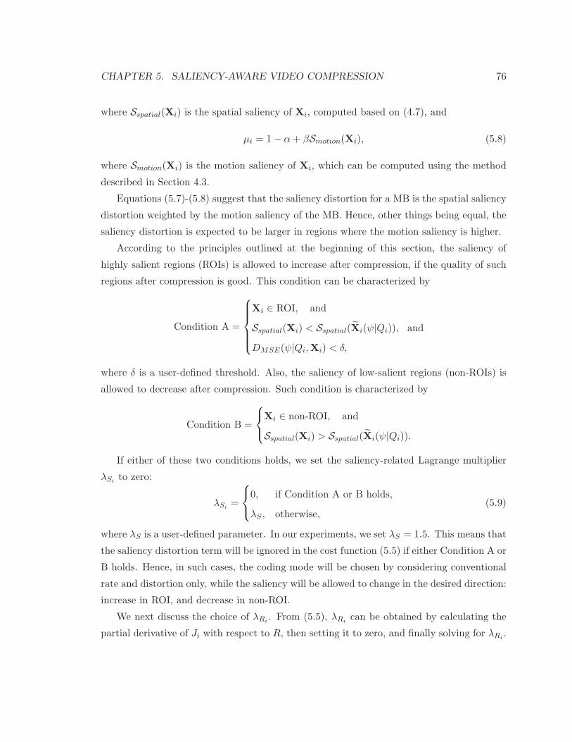
CHAPTER 5. SALIENCY-AWARE VIDEO COMPRESSION 76
where Sspatial(Xi) is the spatial saliency of Xi, computed based on (4.7), and
µi = 1− α+ βSmotion(Xi), (5.8)
where Smotion(Xi) is the motion saliency of Xi, which can be computed using the method
described in Section 4.3.
Equations (5.7)-(5.8) suggest that the saliency distortion for a MB is the spatial saliency
distortion weighted by the motion saliency of the MB. Hence, other things being equal, the
saliency distortion is expected to be larger in regions where the motion saliency is higher.
According to the principles outlined at the beginning of this section, the saliency of
highly salient regions (ROIs) is allowed to increase after compression, if the quality of such
regions after compression is good. This condition can be characterized by
Condition A =
Xi ∈ ROI, and
Sspatial(Xi) < Sspatial(Xi(ψ|Qi)), and
DMSE(ψ|Qi,Xi) < δ,
where δ is a user-defined threshold. Also, the saliency of low-salient regions (non-ROIs) is
allowed to decrease after compression. Such condition is characterized by
Condition B =
Xi ∈ non-ROI, and
Sspatial(Xi) > Sspatial(Xi(ψ|Qi)).
If either of these two conditions holds, we set the saliency-related Lagrange multiplier
λSito zero:
λSi=
0, if Condition A or B holds,
λS , otherwise,(5.9)
where λS is a user-defined parameter. In our experiments, we set λS = 1.5. This means that
the saliency distortion term will be ignored in the cost function (5.5) if either Condition A or
B holds. Hence, in such cases, the coding mode will be chosen by considering conventional
rate and distortion only, while the saliency will be allowed to change in the desired direction:
increase in ROI, and decrease in non-ROI.
We next discuss the choice of λRi. From (5.5), λRi
can be obtained by calculating the
partial derivative of Ji with respect to R, then setting it to zero, and finally solving for λRi.

CHAPTER 5. SALIENCY-AWARE VIDEO COMPRESSION 77
More specifically, we need to have
∂Ji(ψ|Qi, λSi, λRi
,Xi)
∂R(ψ|Qi,Xi)
=∂DMSE(ψ|Qi,Xi)
∂R(ψ|Qi,Xi)+ λSi
∂Dsal(ψ|Qi,Xi)
∂R(ψ|Qi,Xi)+ λRi
= 0.
(5.10)
Solving for λRigives
λRi= −∂DMSE(ψ|Qi,Xi)
∂R(ψ|Qi,Xi)− λSi
∂Dsal(ψ|Qi,Xi)
∂R(ψ|Qi,Xi). (5.11)
With Lagrange multipliers set according to (5.9) and (5.11), the encoder can choose the
optimal coding mode ψ for Xi. We next derive a closed-form expression for λRifor the case
when the transformed residual of Xi obeys a Laplacian model.
5.2.3 Statistical modeling of transformed residuals
Following [135], we model the marginal density of transformed residuals Y by a zero-mean
Laplace probability density function with parameter λ,
fY (y;λ) =λ
2e−λ|y|. (5.12)
The relationship between λ and standard deviation σY is
λ =
√2
σY. (5.13)
To describe the correlation structure of the signal, we adopt a separable autocorrelation
function ri(m,n) = σ2riρ|m|i ρ
|n|i , where m and n are the horizontal and vertical distances
between samples, respectively, σ2ri is the variance of the residual signal of MB Xi before
transformation, and ρi is the correlation coefficient of the residual signal of MB Xi, assumed
to be equal in horizontal and vertical directions. This model is thought to be a good model
for natural digital images [136]. Using such a model, the variance of the (j, l)-th transform
coefficient obtained under coding mode ψ can be obtained as follows [137, 106, 136]
σ2Yi(j, l) = σ2ri [A(ψ)Ki(ψ)A(ψ)T ]j,j [A(ψ)Ki(ψ)A(ψ)T ]l,l, (5.14)
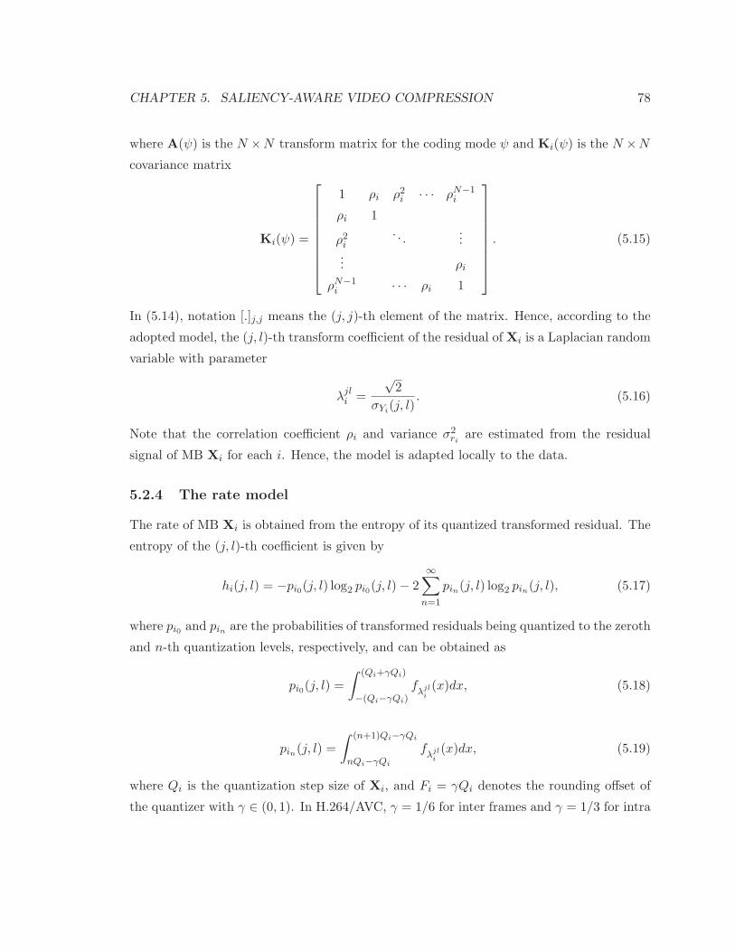
CHAPTER 5. SALIENCY-AWARE VIDEO COMPRESSION 78
where A(ψ) is the N ×N transform matrix for the coding mode ψ and Ki(ψ) is the N ×N
covariance matrix
Ki(ψ) =
1 ρi ρ2i · · · ρN−1i
ρi 1
ρ2i. . .
...... ρi
ρN−1i · · · ρi 1
. (5.15)
In (5.14), notation [.]j,j means the (j, j)-th element of the matrix. Hence, according to the
adopted model, the (j, l)-th transform coefficient of the residual of Xi is a Laplacian random
variable with parameter
λjli =
√2
σYi(j, l)
. (5.16)
Note that the correlation coefficient ρi and variance σ2ri are estimated from the residual
signal of MB Xi for each i. Hence, the model is adapted locally to the data.
5.2.4 The rate model
The rate of MB Xi is obtained from the entropy of its quantized transformed residual. The
entropy of the (j, l)-th coefficient is given by
hi(j, l) = −pi0(j, l) log2 pi0(j, l)− 2∞∑
n=1
pin(j, l) log2 pin(j, l), (5.17)
where pi0 and pin are the probabilities of transformed residuals being quantized to the zeroth
and n-th quantization levels, respectively, and can be obtained as
pi0(j, l) =
∫ (Qi+γQi)
−(Qi−γQi)fλjli
(x)dx, (5.18)
pin(j, l) =
∫ (n+1)Qi−γQi
nQi−γQi
fλjli
(x)dx, (5.19)
where Qi is the quantization step size of Xi, and Fi = γQi denotes the rounding offset of
the quantizer with γ ∈ (0, 1). In H.264/AVC, γ = 1/6 for inter frames and γ = 1/3 for intra

CHAPTER 5. SALIENCY-AWARE VIDEO COMPRESSION 79
frames [115, 114]. The total rate of MB Xi coded under coding mode ψ with quantization
step size Qi can be estimated from the sum of entropies of individual transform coefficients
R(ψ|Qi,Xi) = ζ∑
(j,l)
hi(j, l), (5.20)
where ζ is a factor to compensate for the inaccuracies in the model. For example, the
transform coefficients are assumed to be correlated in Section 5.2.3, which will result in a
lower rate than the sum of their individual entropies. Hence, we expect ζ < 1. In our
experiments, we set ζ = 0.8.
In order to simplify subsequent equations, we define the following symbols for commonly
used quantities:
νjli = λjli Qi
φjli = e−νjli − 1
ξjli = eλjli (Fi−Qi)
ψjli = eν
jli
κjli = (λjli )2QiFi
θjli = λjli ξjli
ηjli = 1− eλjli (Fi−Qi).
(5.21)
Substituting (5.17)-(5.19) into (5.20), using (5.21), we obtain a closed-form expression for
the rate of Xi in (5.22).
R(ψ|Qi,Xi) = − ζ
ln 2
∑
(j,l)
(ξjli
(ln(−φjli )− ln 2 + Fiλ
jli +
νjli
φjli
)+ ηjli ln(ηjli )
). (5.22)
5.2.5 The distortion models
The total MSE distortion in Xi is the sum of quantization distortions contributed by indi-
vidual transform coefficients:
DMSE(ψ|Qi,Xi) =∑
(j,l)
(∫ (Qi+γQi)
−(Qi−γQi)x2f
λjli
(x)dx
+ 2
∞∑
n=1
∫ (n+1)Qi−γQi
nQi−γQi
(x− nQi)2f
λjli
(x)dx).
(5.23)

CHAPTER 5. SALIENCY-AWARE VIDEO COMPRESSION 80
After some algebraic manipulation, DMSE(ψ|Qi,Xi) can be expressed in the closed form as
DMSE(ψ|Qi,Xi) =∑
(j,l)
χjli =
∑
(j,l)
eλjli Fi(2νjli + (νjli )
2 − 2κjli ) + 2− 2ψjli
−φjli (λjli )
2. (5.24)
Based on (5.7), the saliency distortion of a MB is proportional to the spatial saliency
distortion of the MB weighted by the motion saliency of the MB. As described in Section 4.2,
our approximation to the spatial saliency of a MB is the power of the Wiener-filtered DCT
of the MB. In order to estimate the spatial saliency distortion of a block due to quantization,
we model the quantization process by an equivalent quantization noise [138], and consider
the Wiener-weighted energy of the quantization noise in the DCT domain as our spatial
saliency distortion. More specifically, we consider the following expression as a model for
Dsal(ψ|Qi,Xi).
Dsal(ψ|Qi,Xi) = µi∑
(j,l)
H(j, l)χjli , (5.25)
where χjli is as defined in (5.24).
5.2.6 A closed-form expression for λRi
From the expressions for R(ψ|Qi,Xi), DMSE(ψ|Qi,Xi) and Dsal(ψ|Qi,Xi), we can obtain
the expression for λRi. To do this, using the chain rule, we express the ratios in (5.11) in
terms of partial derivatives with respect to Qi,
λRi= −
∂∂Qi
(DMSE(ψ|Qi,Xi) + λSiDsal(ψ|Qi,Xi))
∂∂Qi
R(ψ|Qi,Xi), (5.26)
where the numerator is given in (5.27), and the denominator is given in (5.28).
∂
∂Qi(DMSE(ψ|Qi,Xi) + λSi
Dsal(ψ|Qi,Xi))
=∑
(j,l)
(1 + µiλsH(j, l))
(2λjli ν
jli − eFiλ
jli
(2λjli − 2Fi(λ
jli )
2 + 2(λjli )2Qi
)
(λjli )2(ψjl
i − 1)+
ψjli
(eFiλ
jli
((νjli )
2 − 2Fi(λjli )
2Qi + 2λjli Qi
)− 2νjli + 2
)
λjli (ψjli − 1)2
).
(5.27)

CHAPTER 5. SALIENCY-AWARE VIDEO COMPRESSION 81
∂R(ψ|Qi,Xi)
∂Qi=−ζln 2
∑
(j,l)
θjli
(1 +
(λjliφjli
− λjli
ψjli φ
jli
+(λjli )
2Qi
ψjli (φ
jli )
2
)+ ln(−φjli )−
(ln(−φjli )− ln 2 + Fiλ
jli +
νjli
φjli
)).
(5.28)
Note that several quantities, such as νjli and λjli , appear in both (5.27) and (5.28), which
means that computational effort can be reduced by computing these quantities only once.
In our implementation, we first compute (5.27), and values of the quantities that are shared
with (5.28) are reused.
It is worth pointing out that λRiin (5.26) depends on the content of each MB through
the variance and correlation of the residual of MB Xi, as well as the motion and spatial
saliency of Xi, based on (5.7). Hence, using (5.26), we can adjust the Lagrange multiplier
in a content-adaptive manner on a MB-by-MB basis.
5.3 Experimental results
5.3.1 Objective quality assessment
In order to objectively compare the perceptual quality of video produced by the proposed
saliency-aware video compression method versus that of other methods, we used the eye-
tracking-weighted Mean Square Error (EWMSE) metric proposed in [72]. The EWMSE
value of an encoded video frame can be computed as follows [72]
EWMSE =
∑Wx=1
∑Hy=1
(wx,y · (F ′
x,y − Fx,y)2)
WH∑W
x=1
∑Hy=1wx,y
, (5.29)
where F ′x,y and Fx,y respectively denote the pixel at location (x, y) in the encoded frame F′
and the original frame F, W and H are the width and height of F in pixels, and wx,y is
the weight for distortion at pixel location (x, y), obtained using the following 2-D Gaussian
function
wx,y =1
2πσxσyG
G∑
g=1
exp
−((x− xpg)
2
2σ2x+
(y − ypg)2
2σ2y
), (5.30)
where (xpg , ypg) is the eye fixation position of the g-th subject. We used eye fixation data
from our database in Chapter 3, where the total number of subjects is G = 15. In (5.30), σx

CHAPTER 5. SALIENCY-AWARE VIDEO COMPRESSION 82
and σy are two parameters that specify the width of the Gaussian function, and they depend
on the viewing distance and viewing angle. The values of σx and σy can be taken based on
the fovea size, which is about 2− 5 of visual angle [12], [72]. Here, similar to [12], [72], we
use σx = σy = 64 pixels, which is equivalent to 2 of the visual angle. Using the EWMSE
metric given by (5.29), the eye-tracking-weighted PSNR (EWPSNR) in dB is defined as
EWPSNR = 10 log
(2552
EWMSE
). (5.31)
In our experiments, the average EWPSNR across all frames is considered as one measure
of the perceptual quality of the video - the higher the EWPSNR, the higher the quality of
the encoded video.
In order to evaluate the proposed saliency-aware video compression method, we com-
pared its EWPSNR performance at several bit rates with the conventional RDO method
implemented in the H.264/AVC reference software JM 16.1 [114], as well as two recent
ROI-coding methods: the FJND method proposed in [122] and the visual attention guided
bit allocation (VAGBA) method proposed in [72]. The comparison was made on the 12
sequences from our database in Chapter 3. Higher average EWPSNR is expected if, on av-
erage, the predictions of highly salient regions are closer to the actual human fixation points.
To compute the EWPSNR values, we used the luma (Y) pixel values and the eye-tracking
data of the first viewing in our eye-tracking database.
All videos were encoded by each of the aforementioned methods at different bit rates
with a GOP structure of IPPP. To encode a video at different bit rates, we varied the frame-
level QP (QPf ) of the video between 25 to 40, and at each value, we computed the average
EWPSNR and PSNR of the encoded video. Two sample sets of results, for Foreman and
Tempete, are shown in Fig. 5.1 and 5.2, respectively. In these figures, EWPSNR is plotted
against the bit rate. In these experiments, FJND and VAGBA used IKN-FA saliency maps,
while the proposed saliency-aware coding method used the saliency maps produced by our
GMC saliency estimation method from Section 4.3. As seen in the figures, the proposed
method achieves higher EWPSNR than the other three methods across a range of bit rates.
In the next set of results, we utilized the Bjontegaard Delta (BD) method [139] to mea-
sure the average difference between rate-distortion (RD) curves. We applied this procedure
on both EWPSNR and PSNR curves. To be able to compare the performance of various
methods, we considered the conventional RDO method as the baseline and computed the
average difference of various metrics relative to this baseline.

CHAPTER 5. SALIENCY-AWARE VIDEO COMPRESSION 83
0 100 200 300 400 500 600 70028
30
32
34
36
38
40
Rate (kbps)
EW
PS
NR
(dB
)
Foreman (CIF)
RDOProposedFJNDVAGBA
Figure 5.1: A plot of EWPSNR versus rate for Foreman.
We first compare the various methods in terms of their bit allocation strategy. To
do this, we remove the influence of saliency estimation and its accuracy by using saliency
maps produced by eye-tracking heat maps from the database in Chapter 3. This way,
FJND, VAGBA, and the proposed method use the same saliency maps, which in turn
precisely match the eye-tracking data, leaving bit allocation as the main difference among
the methods. Table 5.1 shows BD-EWPSNR and BD-PSNR results with conventional RDO
method taken as the baseline. As seen from the results, the proposed method is able to
provide an average EWPSNR gain of 2.05 dB with respect to RDO, 1.00 dB (= 2.05 dB
−1.05 dB) with respect to VAGBA, and 0.67 dB (= 2.05 dB −1.38 dB) with respect to
FJND. In terms of conventional PSNR, the average gain of the proposed method is 0.25 dB
(= −0.01 dB +0.26 dB) with respect to FJND, and 0.14 dB (= −0.01 dB +0.15 dB) with
respect to VAGBA, while the average loss against RDO is minimal (0.01 dB). These results
indicate that the bit allocation strategy of the proposed method is more efficient than that
of FJND and VAGBA.
Next, we compare the combination of the proposed methods (that is, the proposed
video coding method coupled with the GMC saliency estimation from Section 4.3) against
the state of the art. As the state of the art, we take FJND and VAGBA coupled with the
IKN-FA saliency model, which was shown as the most accurate in terms of gaze prediction

CHAPTER 5. SALIENCY-AWARE VIDEO COMPRESSION 84
0 500 1000 1500 200024
26
28
30
32
34
36
38
Rate (kbps)
EW
PS
NR
(dB
)
Tempete (CIF)
RDOProposedFJNDVAGBA
Figure 5.2: A plot of EWPSNR versus rate for Tempete.
among the nine tested methods in [92] on the eye-tracking dataset described in Chapter 3.
The methods are compared in terms of BD-EWPNSR, BD-PSNR, BD-SSIM [126], and BD-
VQM [140],[141] in Table 5.2, with RDO taken as the baseline. Note that the lower the
VQM value, the higher the visual quality measured by VQM. As seen from the table, on
average, the proposed methods increase the BD-EWPSNR by 1.45 dB with respect to con-
ventional RDO, while achieving zero average loss in PSNR (BD-PSNR = 0.00). Moreover,
the proposed methods improve the video quality in terms of all metrics (EWPSNR, PSNR,
SSIM, VQM) compared to FJND and VAGBA.
It is interesting to note that RDO performs slightly better, on average, than any of the
perceptually-motivated video coding methods in terms of SSIM and VQM. This is likely due
to the fact that both SSIM and VQM ignore visual attention (i.e., saliency), while SSIM in
addition does not capture temporal aspects of visual quality.
5.3.2 Subjective evaluation
Finally, we performed a subjective evaluation of the perceptual quality of sequences en-
coded using the proposed saliency-aware compression method versus sequences encoded
using FJND [122]. We chose FJND as the competing method here because it performed
slightly better than VAGBA in the tests described above. We utilized a Two Alternative

CHAPTER 5. SALIENCY-AWARE VIDEO COMPRESSION 85
Table 5.1: Comparing the proposed video compression method with the FJND method [122]and the VAGBA method [72] based on the average BD-EWPSNR and BD-PSNR values withrespect to the conventional RDO method when the eye-tracking heatmaps are used as thesaliency maps.
Video FJND [122] VAGBA [72] ProposedBD-EWPSNR BD-PSNR BD-EWPSNR BD-PSNR BD-EWPSNR BD-PSNR
Bus +1.58 −0.21 +1.16 −0.15 +2.16 +0.08City +1.40 −0.27 +1.01 −0.15 +1.98 −0.15Crew +1.53 −0.10 +1.02 −0.07 +1.90 +0.20
Foreman +1.52 −0.31 +0.89 −0.19 +1.98 −0.17Flower Garden +1.77 −0.25 +1.26 −0.11 +2.31 +0.02Hall Monitor +1.33 −0.54 +0.94 −0.29 +1.79 −0.33
Harbor +1.02 −0.19 +1.07 −0.14 +1.95 −0.16Mobile Calendar +1.00 −0.18 +1.15 −0.13 +2.39 +0.31
Mother & Daughter +1.28 −0.37 +0.91 −0.18 +2.03 −0.31Soccer +1.01 −0.13 +0.93 −0.14 +1.88 −0.05Stefan +1.80 −0.39 +1.13 −0.16 +2.04 −0.04Tempete +1.67 −0.15 +1.15 −0.09 +2.21 +0.43
Average +1.38 −0.26 +1.05 −0.15 +2.05 −0.01
Forced Choice (2AFC) method [142] to compare subjective video quality. In 2AFC, the
participant is asked to make a choice between two alternatives, in this case, the video en-
coded using the proposed method vs. video encoded using FJND. This way of comparing
quality is less susceptible to measurement noise than quality ratings based on scale, such as
Mean Opinion Score (MOS) and Double Stimulus Continuous Quality Scale (DSCQS) [143],
because participant’s task is much simpler than mapping quality to a number on the scale.
All 12 CIF sequences from the database in Chapter 3 were used in the experiment. All
sequences were encoded with a GOP structure of IPPP using the two compression methods.
The average PSNR of the encoded videos was around 31 dB, and their bit rates were
matched to within 1% difference. In each trial, participants were shown two videos, side by
side, at the same vertical position separated by 1 cm horizontally on a mid-gray background.
Each video pair was shown for 10 seconds. After this presentation, a mid-gray blank screen
was shown for 5 seconds. During this period, participants were asked to indicate on an
answer sheet, which of the two videos looks better (Left or Right). They were asked to
answer either Left or Right for each video pair, regardless of how certain they were of their
response. Participants did not know which video was produced by the proposed method
and which one was produced by FJND. Randomly chosen half of the trials had the video

CHAPTER 5. SALIENCY-AWARE VIDEO COMPRESSION 86
Table 5.2: Comparing various methods with conventional RDO based on the average BD-EWPSNR, average BD-PSNR, average BD-SSIM, and average BD-VQM values.
FJND [122]Video BD-EWPSNR BD-PSNR BD-SSIM BD-VQMBus +0.28 −0.18 −0.007362 +0.011053City +0.07 −0.09 −0.003250 +0.004384Crew +0.27 −0.08 −0.002006 +0.009742
Foreman +0.19 −0.16 −0.002003 +0.006101Flower Garden +0.60 −0.12 −0.002202 +0.007403Hall Monitor +0.67 −0.12 −0.002378 +0.014506
Harbor +0.13 −0.15 −0.004979 +0.017908Mobile Calendar +0.21 −0.12 −0.003537 +0.009658
Mother & Daughter +0.46 −0.29 −0.004065 +0.016102Soccer +0.23 −0.17 +0.024222 −0.008660Stefan +0.65 −0.12 −0.000593 +0.000102Tempete +0.98 −0.09 −0.003144 +0.009854
Average +0.40 −0.15 −0.003484 +0.010925
VAGBA [72]
Video BD-EWPSNR BD-PSNR BD-SSIM BD-VQMBus +0.37 −0.14 −0.005982 +0.009714City +0.06 −0.15 −0.005329 +0.012298Crew +0.49 −0.13 −0.003320 +0.017451
Foreman +0.48 −0.24 −0.003009 +0.011736Flower Garden +0.81 −0.13 −0.002743 +0.013063Hall Monitor +0.81 −0.13 −0.003006 +0.031234
Harbor +0.28 −0.16 −0.004281 +0.011610Mobile Calendar +0.32 −0.13 −0.003245 +0.004019
Mother & Daughter +0.32 −0.23 −0.002226 +0.006420Soccer +0.54 −0.23 −0.008660 +0.021080Stefan +0.67 −0.13 −0.000863 +0.000119Tempete +0.71 −0.13 −0.002862 +0.009357
Average +0.49 −0.17 −0.003794 +0.012347
Proposed
Video BD-EWPSNR BD-PSNR BD-SSIM BD-VQMBus +0.93 +0.02 −0.002766 0.001434City +1.55 −0.27 −0.014254 +0.028715Crew +0.94 +0.11 +0.001360 +0.005731
Foreman +1.62 −0.11 −0.001289 +0.007552Flower Garden +1.73 +0.14 +0.003143 −0.001978Hall Monitor +1.65 −0.09 −0.002385 +0.017588
Harbor +0.98 −0.12 −0.005621 +0.022322Mobile Calendar +1.50 +0.38 +0.006875 −0.006075
Mother & Daughter +1.54 −0.26 −0.004703 +0.017603Soccer +1.30 −0.31 −0.014136 +0.036290Stefan +1.67 +0.07 +0.001622 −0.000051Tempete +1.95 +0.45 +0.007581 −0.011511
Average +1.45 +0.00 −0.002048 +0.009802
CHAPTER 5. SALIENCY-AWARE VIDEO COMPRESSION 87
produced by the proposed method on the left side of the screen and the other half on the
right side, in order to counteract side bias in the responses. This gave a total of 12 · 2 = 24
trials.
The experiment was run in a quiet room with 15 participants (14 male, 1 female, aged
between 18 and 30). All participants had normal or corrected to normal vision. A 22-inch
Dell monitor with brightness 300 cd/m2 and resolution 1680× 1050 pixels was used in our
experiments. The brightness and contrast of the monitor were set to 75%. The actual height
of the displayed videos on the screen was 185 millimeters. The illumination in the room was
in the range 280-300 Lux. The distance between the monitor and the subjects was fixed at
80 cm. Each participant was familiarized with the task before the start of the experiment
via a short printed instruction sheet. The total length of the experiment for each participant
was approximately 6 minutes.
The results are shown in Table 5.3 in terms of the number of responses that showed
preference for the FJND method vs. the proposed method. To test for statistical signifi-
cance, we used a two-sided χ2-test [144], with the null hypothesis that there is no preference
for either method, i.e., that the votes for each method come from distributions with equal
means. Under this hypothesis, the expected number of votes in each trial is 15 for each
method, because each video pair was shown twice to each of the 15 participants. The p-
value [144] of the test is indicated in the table. As a rule of thumb, the null hypothesis is
rejected when p < 0.05. When this happens in Table 5.3, it means that the two methods
under the comparison cannot be considered to have the same subjective quality, since one of
them has obtained a statistically significantly higher number of votes, and therefore seems
to have better quality.
In 8 out of the 12 cases in Table 5.3 we have p < 0.05, which indicates that subjects
showed a statistically significant preference for the proposed method vs. FJND. In only 4
cases (Bus, Flower Garden, Harbor, and Mobile Calendar) the p-value is larger than 0.05,
which means that neither method achieved a statistically significant advantage. Looking
across all trials (i.e., summing up all the votes for the two methods), the results show that
participants have preferred the proposed method much more than FJND (268 vs. 92 votes)
with overall p = 0.0001, which is a very statistically significant result. This confirms that
the proposed method is able to provide higher perceptual video quality compared to FJND.

CHAPTER 5. SALIENCY-AWARE VIDEO COMPRESSION 88
Table 5.3: Subjective comparison of the proposed video compression method against FJND.
Sequence FJND Proposed p-value
Bus 12 18 0.2733
City 4 26 0.0001
Crew 7 23 0.0035
Foreman 8 22 0.0106
Flower Garden 10 20 0.0679
Hall Monitor 9 21 0.0285
Harbor 11 19 0.1441
Mobile Calendar 10 20 0.0679
Mother & Daughter 4 26 0.0001
Soccer 5 25 0.0003
Stefan 4 26 0.0001
Tempete 8 22 0.0106
Total 92 268 0.0001
5.4 Conclusions
In this chapter, we presented a saliency-aware video compression method in the context of
ROI-based video coding. The proposed method attempts to reduce attention-grabbing cod-
ing artifacts, and further allows the saliency of the encoded video to change in a controlled
manner – increase in ROI and decrease in non-ROI. This is achieved by adding a saliency
distortion term to the distortion metric used in H.264/AVC rate distortion optimization.
The GMC saliency estimation method from Section 4.3 was used to estimate saliency distor-
tion. The results indicate that the proposed method is able to improve the visual quality of
encoded video compared to conventional RDO video coding, as well as two state-of-the-art
perceptually-motivated video coding methods.
Chapter 6
Saliency-Cognizant Video Error
Concealment
Despite ongoing efforts to further advance communication technologies, high quality real-
time video streaming over best-effort, packet-switched networks remains challenging for a
number of reasons. First, consumer demand for interactive streaming video (e.g., conference
video such as Skype, Google Talk, etc.) continues to outpace the rate of increase in network
bandwidth [145], resulting in congestion and packet queue overflows in packet-switched
networks. Second, when packet losses do occur, persistent server-client retransmission is not
practical due to playback constraints – a video packet arriving at decoder past its playback
deadline is essentially useless. Third, new media types such as ultra-high-resolution video
and multiple-view video [146] that promise enhancement of viewing experience are also
further straining resource-limited networks due to their large size. Under these practical
constraints, it is difficult to guarantee error-free delivery of the entire video from sender to
receiver in a timely manner.
Many previous works [147, 148, 149] employed the pro-active methodology of unequal
error protection (UEP) of video data, where important packets are protected more heavily,
for example, using stronger Forward Error Correction (FEC) codes. Typically, more im-
portant packets contain viewer’s probable Regions-of-Interest (ROI) [122] in a video frame,
or regions with higher visual saliency [2], where viewers most likely will focus their visual
attention. In such a scheme, when a packet is lost, the affected region is very likely to be of
low visual saliency. While the loss of high-saliency information is still possible, this is a rare
89
CHAPTER 6. SALIENCY-COGNIZANT VIDEO ERROR CONCEALMENT 90
event compared to the loss of low-saliency information, which is less protected. Instead of
proactive error protection schemes like UEP, in this chapter, we study the complementary
problem of error concealment : given the occasional unavoidable packet loss during network
transmission, causing the loss of a group of macroblocks (MB) in a video frame, how to best
conceal the effect of data loss at the decoder to minimize visual distortion.
Error concealment is typically an under-determined problem: there are insufficient num-
ber of well-defined criteria, such as smoothness conditions for boundary pixels adjacent to
correctly received neighboring blocks [150], to recover all missing MBs perfectly. This makes
choosing the appropriate set of pixels to replace the missing blocks a technically challenging
problem. In this chapter, we propose to add a low-saliency prior to the error concealment
problem as a regularization term. It serves two purposes. First, in ROI-based UEP video
streaming, low-saliency prior is likely the correct side information for the lost block and
helps the client identify the correct replacement block for concealment. Second, in the event
that a perfectly matched block cannot be identified, the low-saliency prior reduces viewer’s
visual attention on the loss-stricken spatial region, resulting in higher overall subjective
quality. At this point, it is appropriate to recall the definition of the word “conceal” from
the Oxford English Dictionary [151], which means to keep from sight; hide; keep (something)
secret; prevent from being known or noticed. In a way, the low-saliency prior tries to make
error concealment live up to its name by attempting to hide damaged blocks from viewers’
attention.
We study the effectiveness of a low-saliency prior in the context of a previously proposed
RECAP error concealment system [152]. RECAP transmits a low-resolution (LR) version
of a video frame alongside the original high-resolution (HR) version, so that if blocks in the
HR version are lost, the correctly-received LR version serves as a template for matching of
suitable replacement blocks from a previously correctly-decoded HR frame. We add a low-
saliency prior to the block identification process, so that only replacement candidate blocks
with good match and low saliency can be selected. To estimate saliency, we employ our
convex approximation to the Itti-Koch-Niebur (IKN) saliency model [2, 67] from Section 4.2.
This makes it possible to formulate low-saliency error concealment as a convex optimization
problem and solve it efficiently using convex optimization techniques. Indeed, the complexity
of the proposed method using the convex saliency approximation can be orders of magnitude
lower compared to our previous concealment method in [1], while the resulting video quality

CHAPTER 6. SALIENCY-COGNIZANT VIDEO ERROR CONCEALMENT 91
is equal or better. Specifically, experimental results show that: i) PSNR of the error-
concealed frames can be increased dramatically – up to 3.6 dB over the original RECAP,
and up to 0.7 dB compared to our earlier method in [1], showing the effectiveness of a
low-saliency prior in the under-determined error concealment problem; and ii) subjective
quality of the repaired video using our proposal, as confirmed by an extensive user study, is
better than the original RECAP.
The outline of the chapter is as follows. We discuss related work in Section 6.1, with an
overview of the RECAP video transmission system [152] and our earlier error concealment
method from [1] in Sections 6.1.1 and 6.1.2, respectively. The new error concealment strategy
with low-saliency prior is presented in Section 6.2.1. In Section 6.2.2 we show how the convex
approximation to IKN saliency from Section 4.2 can be applied to the missing block and its
neighborhood. Finally, experimental results and conclusions are presented in Sections 6.4
and 6.5, respectively.
6.1 Related work
In the last two decades, error resilient video transmission over lossy channels and unreli-
able networks has been studied extensively [147, 148, 149, 153]. One general approach for
recovering lost video data (as well as other kinds of data) is retransmission [153]. Although
retransmission is very effective, it increases transmission latency. For example, a round-trip
time (RTT) of about 200 ms between California and Singapore [152] makes even a single
retransmissions lead to latency that would severely degrade interactivity in applications
such as videoconferencing. It should be mentioned that video streaming is generally able
to tolerate higher latency than videoconferencing, but even streaming clients have finite
playout buffers, which means that the number of possible retransmissions is limited. To
avoid retransmission, another general approach is to use Forward Error Correction (FEC).
A video-specific variant of FEC is Unequal Error Protection (UEP) [154], which provides
stronger protection to more important video data, such as macroblock coding modes and
motion vectors. To handle losses in channels with bursty losses, data interleaving techniques
are typically necessary in both FEC and UEP. However, data interleaving also increases la-
tency [152].

CHAPTER 6. SALIENCY-COGNIZANT VIDEO ERROR CONCEALMENT 92
Another approach to deal with losses in video transmission is decoder-side error con-
cealment. The H.264 video coding standard provides an error resilient feature called Flex-
ible Macroblock Ordering (FMO), which allows macroblocks in slices to be arranged in a
checker-board pattern [155], or other, more advanced, 2-D interleaving patterns [156], for
more effective error concealment. However, such techniques are not effective when an entire
frame is lost. Another technique is Reference Picture Selection (RPS) [153], which can be
used to stop error propagation in video transmission with a reaction time of one RTT. In
RPS, in order to prevent long-term error propagation, the encoder uses only past reference
frames that have been positively acknowledged by the decoder. In [152], a practical solution
for low-latency video communications over lossy networks called RECAP (Receiver Error
Concealment using Acknowledge Preview) was proposed, which improves upon RPS such
that visual quality can be high even when RTT is large. Later in this section, we briefly
describe the RECAP framework, upon which we build our error concealment strategy with
low-saliency prior at the decoder.
In the face of challenging network conditions during real-time video streaming, UEP
strategies protect visually important (salient) regions more heavily. If concealment is done
in a saliency-myopic way, so that the resulting salient features draw attention to the (likely)
imperfectly recovered blocks, it will adversely affect the subjective visual quality. This is one
of the main reasons why we apply the low-saliency prior to the error concealment problem,
so that concealment can be done in a saliency-cognizant manner, resulting in recovered
blocks that do not draw unnecessary attention.
Although we apply our low-saliency prior to the RECAP video transmission system [152]
for concreteness, we believe that low-saliency prior itself has more general applicability to
other ROI-based UEP video streaming systems that may employ other error concealment
tools. For example, in [150], where smoothness condition for boundary pixels is used as one
condition for recovery, low saliency can be an additional requirement to further facilitate
correct block recovery. Note that in our proposed method, we address packet losses in
low-saliency spatial regions because that is the typical case. Packet loss in more heavily
protected highly salient regions, while possible, is a rare case, and hence will not affect
much the average performance of the system, as long as some default concealment scheme
is performed.
Visual saliency—a measure of propensity for drawing visual attention—has been a sub-
ject of intense study in the past decade [2, 157, 85]. While earlier works have applied visual

CHAPTER 6. SALIENCY-COGNIZANT VIDEO ERROR CONCEALMENT 93
Yn+1
clientserverXXn+1 n Xn−1 ...
...LR thumbnails
YYn n−1
UEP1 (ROI)UEP2 (non−ROI)
HR video
Figure 6.1: Overview of RECAP packet loss recovery system.
saliency principles to video compression [67], to the best of our knowledge, we are the first
to apply saliency analysis for error concealment of streaming video. A recent evaluation
of saliency models for gaze prediction in video [92] found that the well-known Itti-Koch-
Niebur (IKN) saliency model [2], enhanced by the temporal features and ‘FancyOne’ feature
integration [67], was the most accurate among the nine methods tested in that study. In
our earlier work on low-saliency error concealment [1], we used the IKN model for saliency
calculation. In this chapter, we utilize our convex approximation to the IKN saliency from
Section 4.2, which allows us to formulate the error concealment problem with low-saliency
prior as a convex optimization problem, leveraging existing polynomial-time convex opti-
mization algorithms for globally optimal solutions. In so doing, as will be shown in Section
6.3 and 6.4, we are able to find far better solutions more computation-efficiently than our
previous work in [1].
6.1.1 RECAP video transmission system
Fig. 6.1 shows an overview of the RECAP video transmission system [152]. The server
compresses HR video into ROI layer and non-ROI layer. Using UEP, the ROI layer is more
heavily protected by stronger FEC than the non-ROI layer. Typically, ROI layer contains
more visually salient objects and accounts for 25% or less of the total area of each frame (to
be discussed in more detail in Section 6.4). Given the relatively small size of the ROI layer,
we will assume it is protected well enough that unrecoverable packet losses, as observed by
the client, take place only in the non-ROI layer.
Along with the encoded HR video, the server also low-pass filters and down-samples HR
frames into LR thumbnails (preview frames) and transmits them with heavy protection. In
practice, the size of a thumbnail is 1/16 (down-sampled by a factor of 4 in both dimensions) of
the size of the HR image, and hence it does not incur much redundant transmission overhead.
For encoding purposes, when there is no loss, the HR video frames are predicted from any
past HR reference frame. However, when a loss is detected, HR video frames are predicted

CHAPTER 6. SALIENCY-COGNIZANT VIDEO ERROR CONCEALMENT 94
only from a positively acknowledged reference frames. In contrast, the LR thumbnails are
always predicted from positively acknowledged LR frames. The key advantage of such
acknowledged thumbnails is that every received thumbnail can be properly decoded.
While data-agnostic FEC suffers from the well-known “cliff” effect, where each block of
FEC-protected source data is either recoverable in its entirety or severely damaged and not
recoverable at all, the thumbnail-based scheme enables a more graceful recovery, where lost
HR video blocks can be partially recovered via block search in previous correctly received
HR reference frame, using the corresponding LR thumbnail as a template. Experimental
results in [152] showed that by transmitting thumbnails, RECAP outperformed FEC-only
schemes. The experimental results in [152] also showed that RECAP outperforms FMO,
especially when all slices in a frame are lost. In fact, the effectiveness of RECAP relies on
three principles [152]. First, as many lost blocks may exist in previously decoded frames
at the decoder, the decoder can exploit the thumbnail frame to search for an appropriate
HR block as a replacement for a missing block. Second, in case an appropriate replacement
block cannot be identified, the decoder can form a coarse reconstruction from the thumbnail
frame. Third, the LR stream does not cost too much overhead as thumbnails are of low
resolution. Also, since the thumbnails are predicted only from acknowledged frames, the
overall reliability of the system is increased.
In this chapter, we employ RECAP as a platform to demonstrate the performance and
effectiveness of our proposed low-saliency prior for video error concealment in loss-corrupted
video streaming. As mentioned before, RECAP is employed only for concreteness, to gen-
erate a number of good candidates to replace a missing block. Our low-saliency prior can
be used in any situation where there is insufficient information to decide among multiple
candidate blocks that could potentially replace a missing block.
6.1.2 Overview of the error concealment method from [1]
In [1], we proposed a saliency-cognizant video error concealment method to study the ef-
fectiveness of a low-saliency prior in the context of error concealment. In that method,
we added a low-saliency prior to the block identification process in RECAP, so that only
replacement candidate blocks with good match and low saliency can be selected. In par-
ticular, we designed and applied four saliency reduction operators iteratively, in order to
reduce the saliency of candidate blocks. These operators were:

CHAPTER 6. SALIENCY-COGNIZANT VIDEO ERROR CONCEALMENT 95
1. A notch filter that suppresses the signal in the normalized frequency range [π/256, π/16];
2. A frequency outlier filter that suppresses large frequency components that are not
present in the neighboring blocks;
3. An intensity and color contrast reduction operator that reduces the contrast (and
therefore also saliency) in the intensity and color channels of the IKN saliency model;
4. A deblocking filter [158], which was observed to often have the effect of reducing the
saliency of the block it is applied to.
These operators were applied on a given RECAP candidate block using the following algo-
rithm:
• Step 1: Set j = 1, where j refers to the index of one the four saliency reduction
operators listed above.
• Step 2: Apply the j-th saliency-reduction operator on the current RECAP block.
• Step 3: Project the result of Step 2 onto the thumbnail block using a project-to-
thumbnail operator to make sure that the low-frequency content of the new candidate
is in good match with the thumbnail block.
• Step 4: Compute the saliency of the new block obtained after Step 3.
• Step 5: Compute a saliency-distortion cost, where the saliency is given by Step 4, and
distortion is obtained by the L2-norm of the difference between the new candidate and
the thumbnail block. If the computed cost is lower than the smallest already-known
saliency-distortion cost, then go to Step 2. Otherwise go to Step 6.
• Step 6: If j < 4, then fetch the original RECAP block again, set j = j + 1, and go
to Step 2. Otherwise end.
The above algorithm was performed on the best K RECAP candidates whose L2-
difference with respect to the thumbnail block was the lowest. In the end, the reconstructed
block whose saliency-distortion cost was the lowest was chosen as the final replacement
block. To compute the saliency of the new block in Step 4, the IKN saliency model was
utilized.
CHAPTER 6. SALIENCY-COGNIZANT VIDEO ERROR CONCEALMENT 96
In the present chapter, we extend this earlier work in two ways. First, the objective
function in the present work is somewhat improved. In the new objective function, we allow
two different weights for the matching to the thumbnail and matching to RECAP candidates.
This enables higher emphasis on low-frequency matching to the thumbnail block, which is
more reliable than RECAP candidate blocks. And second, instead of the IKN model, we
employ our convex approximation to the IKN saliency from Section 4.2, which allows us to
make the objective function convex. With the help of this approximation, we are able to
solve the error concealment problem at a significantly lower computational cost.
6.2 The proposed error concealment method
In this section, we present our proposed video error concealment method. In the sequel,
capital bold letters (e.g., X) denote matrices, lowercase bold letters (e.g., x) denote vectors,
and italic letters (e.g., x or X) represent scalars.
6.2.1 Problem formulation
Consider a video frame F in which some blocks from non-ROI (i.e., low-salient) regions
have been lost. Let X be a lost block of size Nb ×Nb, and N (X) be a w × h window in F,
with w, h ≥ Nb, such that it covers only the available blocks in F (i.e., correctly-decoded
or already-concealed blocks) in the neighborhood of X, as well as the location of X itself.
Let S(N (X)) be a saliency operator that computes the saliency of block X within N (X).
Also, let vec(X) be the vectorization operator that vectorizes its input matrix X in a raster
scan, D be a down-sampling matrix [159], L be a low-pass FIR filter [159], and L be the
high-pass FIR complement of L, i.e. L = I− L, where I is the identity matrix.
Our goal is to reconstruct the missing block X so that the reconstructed block, X, has
low saliency after reconstruction. To achieve this goal, we propose the following algorithm,
which is applied on every lost block in F in a raster-scan order:
• Step 1: Apply the RECAP algorithm on the missing block X to obtain the best K
RECAP HR candidates Rk, k = 1, · · · ,K, whose L2 difference with respect to the LR
thumbnail block T is the lowest.
• Step 2: Compute the 2-D DCT of all available spatial neighbors of X. Let Bl be
a matrix whose entry (i, j) is the DCT coefficient (i, j) with the smallest magnitude

CHAPTER 6. SALIENCY-COGNIZANT VIDEO ERROR CONCEALMENT 97
among all available spatial neighboring blocks of X. Similarly, Let Bu be a matrix
whose entry (i, j) is the DCT coefficient (i, j) with the largest magnitude among all
available spatial neighboring blocks of X.
• Step 3: Given a RECAP candidate block Rk, solve the following minimization prob-
lem to obtain the reconstructed block Xk
Xk = argminX
[S (N (X)) + λ1 ‖DLvec(X)− vec(T)‖22 + λ2
∥∥∥Lvec(X)− Lvec(Rk)∥∥∥2
2
],
subject to Bl ≤ ΦXΦt ≤ Bu,
(6.1)
where λ1 and λ2 are two positive real scalars, ‖.‖2 denotes the L2-norm, and Φ is the
2-D DCT matrix, which is of the same size as X. The down-sampling factor of D is
set to the same down-sampling factor that is used to generate T, and L is used to
avoid aliasing due to down-sampling.
• Step 4: Repeat Step 3 for all the K RECAP candidates. Select the candidate with
the smallest objective function value (6.1) as the final reconstructed block X.
The first term in the objective function in (6.1) measures the saliency of the reconstructed
block within N (X). The minimization of this term ensures that the reconstructed block
has low saliency after reconstruction. At the same time, the constraint defined in (6.1) tries
to eliminate any potential frequency outliers in the reconstructed block by restricting the
frequency content of the reconstructed block to be within the extremes of the frequency
content of its available neighboring blocks. This constraint plays the role of the frequency
outlier filter from our previous approach [1].
The second term of the objective function in (6.1) ensures that the reconstructed block
remains in good match with the thumbnail block, while the third term in (6.1) tries to match
the high-frequency content in the candidate block to that of the RECAP candidate block.
In practice, λ1 should be set to a larger value than λ2. The reason is that the thumbnail
block can be considered as a very reliable side information for the low frequency content of
the missing block, so it makes sense to enforce a very good match to the thumbnail block,
i.e., large λ1. However, the match does not have to be exact, because the thumbnail block
has been quantized and compressed as well, and we do not want to over-fit the low frequency
content of the reconstructed block to the quantized thumbnail.

CHAPTER 6. SALIENCY-COGNIZANT VIDEO ERROR CONCEALMENT 98
Unlike the low-frequency content in the second term in (6.1), we do not have a very
reliable side information for the high-frequency content of the missing block in the third
term in (6.1). All we know comes from the high frequency information of the RECAP
candidate block, which might not be the same as the original high frequency content of the
missing block. Hence, λ2 should be set to a smaller value than λ1. In our experiments,
we used λ1 = 1.5 and λ2 = 0.5. The hope is that saliency consideration will provide
sufficient additional information to reconstruct the high-frequency content of the missing
block reasonably well.
6.2.2 The saliency operator S(N (X))
The error concealment problem formulation in (6.1) involves the saliency operator S(N (X))
that computes the saliency of X within N (X). In our previous work [1], we used the
IKN saliency model as an implementation of S(N (X)). However, this approach has two
disadvantages: (i) it is computationally expensive, as discussed in [103], and (ii) it is non-
convex in X, making it difficult to find the globally optimal solution to (6.1). To solve these
problems, we use our convex approximation to the IKN saliency from Section 4.2. With a
saliency operator S(N (X)) that is convex in X, the optimization problem in (6.1) becomes
convex (the last two terms in the objective function are already convex, as is the constraint),
making it possible to solve (6.1) using a variety methods for convex optimization [160, 161].
As was demonstrated in Section 4.4.1, our convex saliency operator approximates the IKN
saliency very well, yet has an advantage of being simpler to compute and easier to integrate
into various optimization problems.
Equation (4.9) is a convex approximation to the IKN saliency of block X by itself,
regardless of its neighborhood. We now define the operator S(N (X)) that computes the
saliency of X within a neighborhood N (X). Let N (X) be a p×p matrix of pixels in F (with
p > Nb) such that it covers both the Nb × Nb missing block X and parts of the available
8-connected spatial neighbors of X. Hence, the position of N (X) relative to X depends on
the available neighbors of X. In Appendix A, we describe various possible cases for defining
N (X) relative to X. The saliency S(N (X)) is computed as in (4.9), with X replaced by
N (X). Below we show that both the spatial and temporal saliency terms of (4.9) are still
convex in X when X is replaced by N (X).
Let B be a p×p matrix whose elements are all equal to the elements of N (X) except for
the elements whose coordinates coincide with X, which are set to zero. In other words, B is

CHAPTER 6. SALIENCY-COGNIZANT VIDEO ERROR CONCEALMENT 99
a matrix that contains the boundary pixels of N (X) around the missing block X. Fig. 6.2
illustrates X, N (X), and B.
N (X) can be obtained by zero-padding (expanding) X via a matrix expansion opera-
tor, Z(X,N (X)), and adding the resulting matrix to B. The matrix expansion operator,
Z(X,N (X)), zero-pads the Nb×Nb matrix X up to a p×p matrix, Xe, and can be realized
as a linear operation
Xe = Z(X,N (X)) = MXN, (6.2)
where M is a binary matrix of size p × Nb, and N is a binary matrix of size Nb × p, both
of which depend on N (X). The method to derive M and N based on N (X) is given in
Appendix A. Finally, since
N (X) = Xe +B = MXN+B (6.3)
is an affine function of X, it is also convex in X. Due to this, we have that
Sspatial(N (X)) = Sspatial(MXN+B), (6.4)
where Sspatial(·) is computed as in (4.7),
Stemporal(N (X)) = Stemporal(MXN+B), (6.5)
where Stemporal(·) is computed as in (4.8), and
S(N (X)) = Sspatial(N (X)) + αStemporal(N (X)), (6.6)
where α is positive as in (4.9), are all convex in X.
6.2.3 Solving the error concealment problem
By using a saliency operator S(N (X)) that is convex in X, the optimization problem in
equation (6.1) becomes convex. The objective function is the sum of three terms. The first
term is convex in X if the convex saliency operator discussed above is used. The second and
third terms are compositions of vectorization (which is convex [162]), linear filtering, and the
squared L2-norm (which is also convex [161]), making them both convex in X. Finally, the
constraint is a combination of affine functions in X, making it convex in X. Hence, in this
case, a variety of methods for convex optimization [161], such as interior-point, ellipsoid,
subgradient, etc., can be used to solve (6.1). In our expeirments, we used the SeDumi
algorithm available in the cvx Matlab package [163].

CHAPTER 6. SALIENCY-COGNIZANT VIDEO ERROR CONCEALMENT 100
Figure 6.2: An illustration of the missing block X, and matrices N (X) and B. Note thatN (X) covers the missing block X and parts of the available spatial neighbors of X. B isa matrix that contains the boundary pixels of N (X) around the missing block X (light-shaded area around X in this figure). Those elements of B whose coordinates coincide withX are set to zero. The saliency of X is computed within the area covered by N (X). Inthis example, it is assumed that all the 8-connected spatial neighbors of X are available.Depending on the availability of the spatial neighbors of X, the area covered by N (X)changes, as discussed in Appendix A.
6.3 Computational complexity
In Section 6.3.1, we analyze the computational complexity of solving (6.1) when the convex
saliency operator discussed above is used. Following that, in Section 6.3.2 we compare this
complexity against the complexity of our previous method from [1].
6.3.1 Computational complexity of the proposed method
In this section, we estimate the computational cost of the error concealment method pre-
sented in Section 6.2.1. In the proposed method, the minimization problem defined in (6.1)
is solved for the best K RECAP candidates whose L2 difference with respect to the thumb-
nail block is the lowest. In the end, the best block whose saliency-distortion cost in (6.1) is
the lowest, is taken as the concealed block.
To estimate the computational cost, we need to answer two questions: 1) how many
evaluations of the objective function in (6.1) are needed? and 2) how many operations are
required in each evaluation of the objective function in (6.1)? The first question is difficult
to answer in general. As mentioned in Section 6.2.3, a convex optimization problem can be
solved relatively easily (in polynomial time) by various convex optimization methods such
as interior-point and ellipsoid methods [160, 161]. However, the exact number of objective

CHAPTER 6. SALIENCY-COGNIZANT VIDEO ERROR CONCEALMENT 101
function evaluations is not easily determined. In our experiments we found that usually
about 8 objective function evaluations are needed to achieve an acceptable tolerance level
of ǫ = 10−6 when solving (6.1) for 16 × 16 blocks. Hence, for the purpose of estimating
complexity, we assume that the average number of objective function evaluations in (6.1) is
Ne = 8.
We now compute the number of operations that are performed in one evaluation of the
objective function in (6.1). To find the cost for the first term in (6.1), we need to find
the cost of the saliency operator S(N (X)) defined in (6.6), which involves in computing
Sspatial(N (X)) and Stemporal(N (X)). The first step in computing Sspatial(N (X)) is to con-
struct N (X). In practice, N (X) can be constructed by copying the Nb×Nb block X to the
zero locations of the p× p matrix B (i.e., locations in which the elements of B are zero). To
copy a Nb ×Nb matrix to another place in memory, we need to update the pointer address
of both the source and destination locations after reading/copying each row of the matrix.
To obtain the pointer address of the next row of the matrix, we first need to increase the
current row number by one, and then the convert the 2-D address of the first element of
next row into a linear 1-D address. This needs 3 operations (two additions and one multi-
plication) [164]. Hence, we consider approximately 2 · 3Nb = 6Nb operations for copying a
Nb × Nb matrix to another place in memory. Assuming that B is available before solving
(6.1), copying the X to the zero locations of B needs approximately 6Nb operations.
The next step is to compute the 2-D DCT of N (X). Note that the multiplication of a
A×B matrix by a B ×C matrix requires A ·C · (2B − 1) operations. Also, computing the
2-D DCT of a p× p block requires two p× p matrix multiplications. Hence, computing the
2-D DCT of N (X) requires 2p2(2p − 1) operations. We then need to compute the square
of the Wiener-filtered coefficients. This step needs 2p2 operations. Finally, all the squared
Wiener-filtered coefficients should be summed up together. This step needs approximately
p2 operations. Hence, computing Sspatial(N (X)) in the luma (Y) channel of X requires
approximately 6Nb + p2(4p+ 1) operations. Assuming that X is in YUV 4:2:0 format, the
total computational cost for computing Sspatial(N (X)) will be 1.5(6Nb + p2(4p+ 1)).
To compute Stemporal(N (X)), we first need to compute the absolute difference between
N (X) and the co-located p × p block in the previous frame in the luma (Y) channel. For
this purpose, we need to construct the neighborhood in the previous frame similar to N (X).
This approximately needs 6Nb operations. Note that N (X) is already constructed when
computing Sspatial(N (X)). Thus, this step requires about 6Nb + 2p2 operations, where we

CHAPTER 6. SALIENCY-COGNIZANT VIDEO ERROR CONCEALMENT 102
considered two operations for computing the absolute difference between two elements of
memory. We then need to compute the 2-D DCT of the obtained residual block, which re-
quires 2p2(2p−1) operations. After that we need to compute the sum of the squared Wiener-
filtered coefficients of the residual block, which requires approximately 2p2 + p2 operations.
Hence, computing Stemporal(N (X)) requires approximately 2p2(2p + 3) operations. Based
on the above analysis, computing S(N (X)) requires approximately 9Nb + p2(10p+ 7.5) + 2
operations.
To find the computational cost of the second and third terms in (6.1), we first note that
if the size of X in (6.1) is Nb × Nb, then L and L are both of size N2b × N2
b , while D (the
down-sampling matrix) is a (N2b /d
2s)×N2
b matrix, where ds is the down-sampling factor that
is used to generate the thumbnail block T. To vectorize a Nb×Nb matrix, similar to the case
discussed above for copying a Nb×Nb block to another location in the memory, we consider
about 6Nb operations. Hence, to obtain vec(Rk) or vec(X), we consider approximately 6Nb
operations. Similarly, we approximate the cost for obtaining vec(T) by 6Nb/ds operations.
To compute DLvec(X) for evaluating the second term in (6.1), we can first compute
Lvec(X), which requires N2b (2N
2b − 1) operations. We can then multiply D by the resul-
tant N2b × 1 vector. This requires additional N2
b (2N2b − 1)/d2s operations. Hence, in total,
computing DLvec(X) costs N2b (2N
2b − 1) +N2
b (2N2b − 1)/d2s + 6Nb operations.
As a simpler alternative, however, the low-pass filtering can be performed in the DCT
domain. For this purpose, we first compute the 2-D DCT of X, which needs 2N2b (2Nb − 1)
operations. We then zero out the desired high frequency coefficients. This process needs
approximately N2b operations. We then take the inverse 2-D DCT of the obtained result
to get the filtered block in the pixel domain. This step needs 2N2b (2Nb − 1) additional
operations. Finally, we down-sample the obtained block by a down-sampling factor ds to
get a down-sampled block of the same size as T. We consider N2b /d
2s operations for this
step. Finally, the L2-norm of the difference between the obtained low-resolution block and
T must be calculated. This step requires approximately 3N2b /d
2s operations. Therefore, in
total, computing the second term of (6.1) in the luma (Y) channel requires approximately
N2b (8Nb − 3 + 4/d2s) operations.
For computing the third term in (6.1), a similar approach can be utilized. Specifically, we
take the 2-D DCT of both X and Rk, and compute the L2-norm of the difference between
the high frequency coefficients of X and Rk. To compute the L2-norm, only those high
frequency DCT coefficients that are zeroed out when computing the second term of (6.1)

CHAPTER 6. SALIENCY-COGNIZANT VIDEO ERROR CONCEALMENT 103
are utilized. Note that since DCT is a unitary transform, we do not need to take the inverse
2-D DCT to compute the L2-norm difference in the pixel domain. The 2-D DCT of X is
available after computing the second term in (6.1). Thus, we only need to compute the
2-D DCT of Rk, which can be pre-computed before evaluating (6.1). Considering 3N2b
operations for computing the L2-norm, computing the third term in (6.1) in the luma (Y)
channel requires approximately 3N2b operations.
In summary, we conclude that computing the second term in (6.1) for all three YUV
4:2:0 channels of X in each evaluation of the objective function requires approximately
1.5 ·(N2b (8Nb−3+4/d2s) operations. For the third term, the cost is approximately 1.5 ·(3N2
b )
operations.
To evaluate the constraint in (6.1), we need to compare the 2-D DCT of X with both
Bl and Bu. For these two comparisons, we consider 2N2b operations. The 2-D DCT of X
is computed during the evaluation of the second term in (6.1) as described above. Hence,
assuming that Bl and Bu are pre-computed before solving (6.1), evaluating the constraint
for all three YUV 4:2:0 channels of X requires 1.5 · (2N2b ) = 3N2
b operations.
Before evaluating (6.1), we need to compute the 2-D DCT of Rk, which requires 1.5 ·2N2
b · (2Nb − 1) operations. We also need to compute Bl and Bu. Assuming the worst
case (from the point of view of complexity) that all the four spatial neighbors of X are
available, and that none of them are neighbors of any previously concealed blocks (in which
case their 2-D DCT would already be available), we need to compute the 2-D DCT of all
four neighbors. This requires 1.5 · 4 · 2N2b (2Nb − 1) operations. Assuming that finding the
minimum or maximum of 4 DCT coefficients needs 3 operations, we can estimate the cost
for computing Bl or Bu as 1.5·3N2b = 4.5N2
b operations. Hence, the total cost for computing
Rk, Bl, and Bu is approximately N2b (30Nb − 11) operations.
Overall, for the YUV 4:2:0 video format, the total computational cost of the proposed
error concealment method for reconstructing a Nb×Nb block X within a p×p neighborhoodN (X) is approximately
ζ(PM) ≈ N2b (30Nb − 11) +Ne
((9Nb + p2(10p+ 7.5) + 2)+
1.5(N2b (8Nb − 3 +
4
d2s)) + 3N2
b
)
= N2b (30Nb − 11) +Ne
(12N3
b − 1.5N2b + 9Nb +
6
d2s+ 10p3 + 7.5p2 + 2
).
(6.7)

CHAPTER 6. SALIENCY-COGNIZANT VIDEO ERROR CONCEALMENT 104
6.3.2 Comparison with the method from [1]
In our experiments, the size of each missing block X is 16 × 16. Therefore, Nb = 16. We
also set ds = 4 and p = 20 so that the window N (X) covers a 20 × 20 region. With these
parameters in (6.7), we get
ζ(PM) ≈ 1175379. (6.8)
Meanwhile, our previous error concealment method from [1] requires the computation
of IKN saliency [67] within an adaptive window of size W0 ×H0 that includes the missing
block and its causal spatial neighborhood. As discussed in [103], the number of operations
required to reconstruct a missing block of size Nb ×Nb pixels by our previous method in [1]
is
ζ(OM) ≈ 36.56N3b +
(log2
N6b
4 + 1104.5)N2
b + 5882 ·W0 ·H0. (6.9)
Substituting Nb = 16 we obtain
ζ(OM) ≈ 438133 + 5882 ·W0 ·H0. (6.10)
Note that W0 and H0 can be as small as Nb, the size of the block, or as large as W and
H, the width and height of the frame. The number of operations involved in reconstructing
a block varies depending on the position of that block, which determines W0 and H0 [1].
At the low end, when W0 = H0 = Nb = 16, ζ(PM) ≈ 0.60 · ζ(OM), making the proposed
method roughly 40% less costly than the method from [1]. At the high end, when W0 and
H0 are equal to the dimensions of the frame, then even for a CIF resolution of 352 × 288
(which may be considered small by today’s standards), we obtain ζ(PM) ≈ 0.002 · ζ(OM).
Hence, in this case, the proposed method has only 1/500-th of cost of the method from [1].
In practice, the computational savings will be somewhere between these two extreme values.
To get a feeling for the average case, consider CIF resolution video (352× 288). Assuming
that each block is equally likely to be damaged, the expected (average) position of the
damaged block is at the center of the frame, and the expected values of W0 and H0 are
352/2 = 176 and 288/2 = 144, respectively. Using these values in (6.10) and comparing
the result with ζ(PM), we find ζ(PM) ≈ 0.008 · ζ(OM). That is, the expected cost of the
proposed method in the case of CIF resolution video is about 1/120-th of that in [1].

CHAPTER 6. SALIENCY-COGNIZANT VIDEO ERROR CONCEALMENT 105
6.4 Experimental results
In this section, we evaluate the performance of the saliency-cognizant error concealment
method from Section 6.2.1 by comparing it with the original RECAP algorithm, as well as
our previous error concealment method from [1].
In order to evaluate the performance of the proposed error concealment method, we
used four standard 30 fps sequences: Soccer (704 × 576), RaceHorses (416 × 240), Tractor
(768 × 432), and Crew (704 × 576). All sequences were 250 frames long. RaceHorses was
encoded at 700 kbps, while the other three higher-resolution sequences were encoded at 1400
kbps using the H.264/AVC JM 18.0 reference software [114], with the GOP structure IPPP.
The thumbnail videos were created by down-sampling their corresponding high resolution
(HR) videos by a factor of 4 in each dimension, and were encoded at 10% of the bitrate of
their HR version, using the same encoder structure as their HR version. We set Nb = 16,
p = 20, α = 1, λ1 = 1.5 and λ2 = 0.5.
In order to find the most salient regions (ROIs), we first computed the full IKN saliency
map of each video frame of each sequence. The saliency map of each frame was then
binarized based on the 75-th percentile of the saliency map of that frame. Macroblocks with
saliency above the 75-th percentile threshold were considered as ROIs.
To simulate a video streaming scenario with RECAP as its error control mechanism,
a video frame was selected randomly, and its macroblocks in non-ROI parts were dropped
randomly based on a two-state Gilbert model [165] at two different average loss rates (3%
and 10%) with an average burst loss length of 8. The corrupted frame was then concealed
using the original RECAP algorithm, our previous error concealment method from [1], as
well as our proposed error concealment method from Section 6.2.1. The RECAP method,
as well as the two other error concealment methods, require a correctly-received reference
frame to generate RECAP candidates. This was assumed to be either 5 or 10 frames away.
In practice, the distance between the concealed and reference frame is random. We used 5
and 10 simply as representative test values. This procedure was repeated on about 30% of
the randomly chosen frames from each sequence.
6.4.1 Objective quality assessment
In Table 6.1, we compared the performance of the proposed error concealment method
with the RECAP method and our earlier error concealment method from [1] at 3% loss

CHAPTER 6. SALIENCY-COGNIZANT VIDEO ERROR CONCEALMENT 106
Table 6.1: Comparing the proposed error concealment method with RECAP and [1], usingvarious image/video quality assessment methods, at 3% loss rate, and at two reference framedistances: d = 10 and d = 5.
Soccer RaceHorsesd Metric RECAP [1] Proposed RECAP [1] Proposed
PSNR 34.6 35.3 35.5 37.6 38.0 38.210 SSIM 0.943254 0.944754 0.946126 0.978554 0.979591 0.980300
VQM 0.204069 0.161319 0.157103 0.088587 0.081535 0.080902PSNR 35.7 36.1 36.2 38.3 38.5 38.9
5 SSIM 0.955522 0.956073 0.956709 0.990184 0.992794 0.993050VQM 0.168544 0.153910 0.139484 0.077677 0.077879 0.077382
Tractor Crewd Metric RECAP [1] Proposed RECAP [1] Proposed
PSNR 32.4 33.8 34.2 35.1 38.2 38.410 SSIM 0.930999 0.940424 0.943242 0.956591 0.969242 0.970139
VQM 0.170746 0.139316 0.138356 0.217980 0.148807 0.148376PSNR 34.2 34.3 35.0 36.5 38.6 38.9
5 SSIM 0.973539 0.981457 0.982164 0.965405 0.972251 0.973920VQM 0.125716 0.126531 0.125092 0.185925 0.137344 0.136188
Table 6.2: Comparing the proposed error concealment method with RECAP and [1] basedon various image/video quality assessment methods, at 10% loss rate, and at two differentreference frame distances: d = 10 and d = 5.
Soccer RaceHorsesd Metric RECAP [1] Proposed RECAP [1] Proposed
PSNR 30.1 31.0 31.2 28.5 28.9 29.110 SSIM 0.847758 0.854268 0.855404 0.857703 0.863775 0.866455
VQM 0.413155 0.339648 0.313936 0.326603 0.264199 0.240614PSNR 31.1 31.5 31.6 29.1 29.5 29.7
5 SSIM 0.874573 0.875573 0.876853 0.878562 0.883668 0.885283VQM 0.366916 0.315949 0.305230 0.276700 0.238212 0.235563
Tractor Crewd Metric RECAP [1] Proposed RECAP [1] Proposed
PSNR 27.2 28.9 29.0 29.8 33.2 33.410 SSIM 0.790720 0.822753 0.822901 0.867791 0.904089 0.904329
VQM 0.271512 0.225952 0.223710 0.363882 0.292193 0.253789PSNR 30.0 30.4 30.5 31.1 33.3 33.6
5 SSIM 0.905805 0.906624 0.910247 0.890988 0.908552 0.910276VQM 0.248732 0.220100 0.203267 0.320792 0.261871 0.241848

CHAPTER 6. SALIENCY-COGNIZANT VIDEO ERROR CONCEALMENT 107
rate, and at two reference frame distances, d = 5 and d = 10, based on three metrics:
PSNR, SSIM [126], and VQM [140, 141]. These frame-level metrics were computed at the
aforementioned average loss rates on the concealed frames. The general VQM model [140]
was utilized for computing the VQM values. Only the luma (Y) channel was considered for
computing the PSNR and SSIM values. Table 6.2 shows the results for the same comparison
as in Table 6.1 but at an average loss rate of 10%.
As seen from Table 6.1 and Table 6.2, the proposed method is able to improve the PSNR
of the concealed frames by up to 3.6 dB compared to RECAP (Crew with d = 10 at 10%
loss rate), and by up to 0.7 dB compared to our earlier method from [1] (Tractor with d = 5
at 3% loss rate). This shows that the proposed error concealment method is able to provide
correct side information for resolving the ambiguity in reconstructing the missing blocks
in the under-determined problem of error concealment. As seen from the SSIM and VQM
results, the proposed error concealment method provides better quality than the RECAP
method. Note that the smaller the VQM value, the better the quality. We also note that
the objective quality of the proposed error concealment method as measured by the SSIM
and VQM metrics is close to or better than our earlier method from [1].
The results demonstrate that even though our earlier method in [1] used the actual IKN
saliency while the method proposed here uses only an approximation, we are able to improve
upon the results from [1]. This is because the present error concealment formulation in (6.1)
allows for direct search for the missing block X, whereas in [1], the concealment proceeded
indirectly by applying saliency reduction operators, in an iterative fashion, upon RECAP
candidate blocks. This, combined with the non-convexity of the objective function from [1],
made the algorithm in [1] susceptible to getting stuck in a local optimum. The present
algorithm does not have that problem, and it is computationally more efficient.
6.4.2 Subjective evaluation
Since the proposed error concealment method aims at reducing the saliency of concealed
blocks, we performed a subjective test to verify the improvement in subjective quality. For
this purpose, we compared the subjective quality of the proposed error concealment method
with RECAP, as well as our earlier method from [1].
In our experiment, a Two Alternative Forced Choice (2AFC) method [142] was used
to compare subjective video quality. In 2AFC, the participant is asked to make a choice
between two alternatives, in this case, the proposed method vs. either the original RECAP

CHAPTER 6. SALIENCY-COGNIZANT VIDEO ERROR CONCEALMENT 108
method or our earlier method [1]. This way of comparing quality is less susceptible to
measurement noise than quality ratings based on scale, such as Mean Opinion Score (MOS)
and Double Stimulus Continuous Quality Scale (DSCQS) [143], because participant’s task
is much simpler than mapping quality to a number on the scale.
Four test sequences mentioned above, at two loss rates (3% and 10%) were used in the
experiment. In each trial, participants were looking at two side-by-side videos (in the same
vertical position, separated by 1 cm horizontally) on a mid-gray background. Each video
pair was shown for 9 seconds. After this presentation, a mid-gray blank screen was shown
for 5 seconds. During this period, participants were asked to indicate on an answer sheet,
which of the two videos looks better (Left or Right). They were asked to answer either
Left or Right for each video pair, regardless of how certain they were of their response.
Participants did not know which video was obtained by the proposed method and which
one was obtained by the alternative method (RECAP or [1]). Randomly chosen half of the
trials had the video produced by the proposed method on the left side of the screen and the
other half on the right side, in order to counteract side bias in the responses. This gave a
total of 4 · 2 · 2 = 16 trials for comparing the proposed error concealment method with each
of the alternative methods.
The experiment was run in a quiet room with 15 participants (11 male, 4 female, aged
between 18 and 30). All participants had normal or corrected to normal vision. A 22-inch
Dell monitor with brightness 300 cd/m2 and resolution 1680× 1050 pixels was used in our
experiments. The brightness and contrast of the monitor were set to 75%. The actual height
of the displayed videos on the screen was 185 millimeters. The illumination in the room was
in the range 280-300 Lux. The distance between the monitor and the subjects was fixed at
80 cm. Each participant was familiarized with the task before the start of the experiment
via a short printed instruction sheet. The total length of the experiment for each participant
was approximately 8 minutes.
The results for the comparison between the RECAP method and our proposed error
concealment method are shown in Tables 6.3 and 6.4. In Table 6.3 we show the number of
responses that showed preference for the original RECAP method vs. the proposed method,
and in Table 6.4 we show the votes for the method from [1] vs. the proposed one.
To test for statistical significance, we used a two-sided χ2-test [144], with the null hy-
pothesis that there is no preference for either method, i.e., that the votes for each method
come from distributions with equal means. Under this hypothesis, the expected number of

CHAPTER 6. SALIENCY-COGNIZANT VIDEO ERROR CONCEALMENT 109
Table 6.3: Subjective comparison of the proposed method against RECAP.
Loss Rate Method Crew Soccer Tractor RaceHorsesRECAP 2 6 6 3
3% Proposed 28 24 24 27p-value 0.0001 0.0010 0.0010 0.0001RECAP 1 5 8 4
10% Proposed 29 25 22 26p-value 0.0001 0.0003 0.0106 0.0001
Table 6.4: Subjective comparison of the proposed method against the method from [1].
Loss Rate Method Crew Soccer Tractor RaceHorses[1] 11 9 10 12
3% Proposed 19 21 20 18p-value 0.1441 0.0285 0.0679 0.2733
[1] 17 10 16 1410% Proposed 13 20 14 16
p-value 0.4652 0.0679 0.7150 0.7150
votes is 15 for each method under study. The p-value [144] of the test is indicated in the
two tables. As a rule of thumb, the null hypothesis is rejected when p < 0.05. When this
happens in Table 6.3 or 6.4, it means that the two methods under the comparison cannot be
considered to have the same subjective quality, since one of them has obtained a statistically
significantly higher number of votes, and therefore seems to have better quality.
In all of the 16 trials in Table 6.3 we have p < 0.05, which indicates that subjects showed
a statistically significant preference for the proposed method vs. RECAP. Looking across all
trials (i.e., summing up all the votes for the two options), the results show that participants
have preferred the proposed method much more than RECAP (205 vs. 35 votes) with overall
p = 0.0001, which is a very statistically significant result. This confirms that the proposed
method is able to improve the perceptual quality of the concealed frames compared to the
original RECAP method.
In Table 6.4, in all of the 16 trials except for one (Soccer at 3%) we have p > 0.05.
This indicates that the subjective quality of the proposed error concealment method is
statistically indistinguishable from our earlier method in [1] at the significance level p = 0.05
on all videos except for Soccer at 3% loss rate, where the result is significant in favor of the
proposed method.

CHAPTER 6. SALIENCY-COGNIZANT VIDEO ERROR CONCEALMENT 110
Fig. 6.3 shows a frame from the sequence Crew concealed by the three methods (RE-
CAP, [1], and the proposed) based on a reference frame that is 10 frames away. One can
easily see that our new method is able to improve the visual quality of the concealed frames
compared to RECAP method, while the differences between the frames produced by the
newly proposed method and that in [1] are harder to see. Indeed, this is to be expected, since
both methods operate on similar principles by trying to reduce the saliency of concealed
blocks.
6.5 Conclusions
Error concealment in loss-corrupted streaming video is a challenging under-determined prob-
lem. In the method described in this chapter, we add a low-saliency prior as a regularization
term to the replacement block search problem. Low saliency provides the correct side infor-
mation in ROI-based UEP video streaming systems for client to identify correct replacement
blocks for concealment. Also, low saliency reduces viewer’s visual attention on the loss-
stricken regions. Incorporated into a previously proposed RECAP error concealment setup,
our experimental results show that our method can clearly improve the visual quality of the
loss-corrupted frames both objectively (up to 3.6 dB in PSNR) and subjectively. Moreover,
incorporating the newly-developed convex approximation to visual saliency into the error
concealment process results in expected complexity reduction of two orders of magnitude
for CIF resolution video, while at the same time providing a gain of up to 0.7 dB in PSNR
compared to an earlier version of the algorithm. Although we utilized RECAP as a plat-
form to demonstrate the performance and effectiveness of our proposed low-saliency prior
for video error concealment, other concealment methods can also benefit from the notion
of a low-saliency prior. In fact, the low-saliency prior can be utilized by any video error
concealment method that can offer multiple candidates for reconstructing missing blocks so
as to reduce the ambiguity in the selection of correct blocks.

CHAPTER 6. SALIENCY-COGNIZANT VIDEO ERROR CONCEALMENT 111
(a) (b)
(c) (d)
Figure 6.3: A frame from Crew : (a) original frame (b) the frame reconstructed by RECAP(PSNR = 34.3 dB) (c) the frame reconstructed by the method from [1] (PSNR = 36.6 dB)(d) the frame reconstructed by the proposed method (PSNR = 36.8 dB).

Chapter 7
Conclusions and Future Directions
7.1 Summary of contributions
In this dissertation, we presented various novel methods for utilizing visual saliency in
the context of video compression and transmission. Specifically, we presented two novel
computationally-efficient saliency estimation methods inspired by the well-known IKN saliency
model. The first method is a convex approximation to the IKN saliency model, consisting of
a spatial and a temporal component. Its spatial component can be used to estimate visual
saliency in static images, while the two components together can be used to estimate the
saliency in video. The computational cost of the spatial component is about 1/11-th of the
complexity of the IKN model for images, while the combined complexity of the spatial and
temporal components is about 1/9-th of that of the IKN model for video. The convexity
of this approximation makes it very attractive to incorporate within various optimization
procedures in image and video processing.
The second proposed saliency estimation method uses the spatial component from the
convex approximation mentioned above, but improves temporal saliency estimation via
global motion compensation. Overall, this method is not convex, but is more accurate than
the IKN saliency model on certain sequences with camera motion. This method uses mo-
tion vectors to accomplish global motion compensation and subsequently temporal saliency
estimation, so it can be very attractive for video compression applications where motion
vectors are readily available. The complexity of this method is about 1/6-th of that of the
IKN model for video.
112
CHAPTER 7. CONCLUSIONS AND FUTURE DIRECTIONS 113
During the course of this research, we also developed an eye-tracking dataset for a num-
ber of standard video sequences that are commonly used in the field of video compression and
transmission. This dataset is publicly available online, and can be utilized for benchmark-
ing and evaluation of visual saliency models and perceptually-motivated video processing
algorithms as well as video quality assessment methods.
In the context of video compression, we presented a novel saliency-aware video com-
pression method within a region-of-interest (ROI) video coding framework. In ROI-based
video coding, ROIs are encoded with higher quality compared to non-ROIs. Hence, various
coding artifacts may be produced in non-ROI parts, especially at low bit rates. Such cod-
ing artifacts may become attention-grabbing (visually salient), and draw viewer’s attention
away from ROI parts. This may degrade the perceived video quality as the visual quality in
non-ROI parts is lower. The proposed saliency-aware video compression method attempts
to reduce such attention-grabbing coding artifacts in non-ROI parts so as to keep viewer’s
attention on ROI parts. At the same time, the proposed method allows saliency to increase
in high quality ROI parts of the frame, and decrease in non-ROI parts. It was demon-
strated that the proposed method achieves higher video quality compared to conventional
rate-distortion optimization, as well as two recent psychovisually-motivated video coding
methods from the literature.
In the context of video transmission, we presented a novel saliency-cognizant video error
concealment method for ROI-based video streaming. In ROI-based transmission, ROIs are
protected more heavily than non-ROI parts, for example, using stronger channel codes. This
way, if errors or losses occur during transmission, the affected regions will most likely be
from non-ROI parts, and so they will be of low visual saliency. Hence, the reconstruction of
the corrupted regions should be such that they end up with low visual saliency after error
concealment; otherwise, if their saliency increases, they may grab viewer’s attention and
thereby degrade visual quality. To achieve this goal, we added a low saliency prior to the
under-determined problem of error concealment. Such a prior serves two purposes. First,
in ROI-based video streaming, low-saliency prior is likely the correct side information for
reconstructing the lost block and helps the client identify the correct replacement block
for concealment. Second, in the event that a perfectly matched block cannot be identified,
the low-saliency prior reduces viewer’s visual attention on the reconstructed region, and so
the overall subjective quality of the reconstructed frame is increased. It was shown that
this strategy leads to improved video quality of concealed frames, both objectively and

CHAPTER 7. CONCLUSIONS AND FUTURE DIRECTIONS 114
subjectively.
7.2 Future directions
Having summarized the contributions of this dissertation, we now outline several possible
directions for future research.
In our proposed global motion-compensated saliency detection method we used a global
motion compensation process to obtain the motion saliency of a video frame. The employed
global motion compensation method uses only the motion vectors of the video frame. Better
results, however, can be achieved if more compressed-domain information such as block
coding (partition) mode is used for global motion compensation [166]. In particular, a
motion segmentation and object tracking approach like the recent method proposed in [166]
can be used to dynamically track foreground objects across different frames. The method
in [166] uses both motion vectors and block coding modes to segment and track foreground
objects by the help of a spatio-temporal Markov Random Field (ST-MRF) model. Hence,
as a future work, we can use a method like [166] to improve our proposed GMC saliency
detection method as well as our proposed saliency-aware video compression method.
In our proposed saliency-aware video compression method, we combined a saliency dis-
tortion term with the conventional MSE distortion metric. As a possible future work, the
conventional MSE distortion metric can be replaced by a more perceptually-relevant distor-
tion metric such as SSIM to achieve even better results. For instance, the reduced-reference
SSIM estimation method proposed in [130] can be utilized in conjunction with the proposed
saliency distortion metric to achieve better perceptual quality in video compression. Also,
in Section 5.2.2, we set the saliency-related Lagrange multiplier λSibased on (5.9) to either
zero, or an experimentally determined value of 1.5. However, further adaptation of this La-
grange multiplier can be introduced based on the saliency of each macroblock. For example,
the value of λS can be increased in ROI parts to emphasize the effect of saliency distortion
in these regions.
Our proposed saliency-cognizant error concealment method attempts to reduce the
saliency of the reconstructed regions in non-ROI parts of the frame so that the visual atten-
tion is not directed towards the reconstructed regions. As a future direction for improving
our proposed saliency-cognizant error concealment method, an efficient method can be de-
signed to deliberately increase the saliency of ROI parts of the frame after performing the

CHAPTER 7. CONCLUSIONS AND FUTURE DIRECTIONS 115
proposed error concealment method to make sure that the visual attention is directed away
from the reconstructed regions as much as possible. For instance, the attention-guiding
method from [167] can be utilized to further increase the visual saliency of ROI parts of the
video frame. In particular, the saliency adjustment can be performed in such a way that
the objective or perceptual quality of the manipulated ROI parts is not degraded too much.
This can possibly be achieved by adding a distortion metric (e.g., MSE or SSIM) to the
saliency adjustment process as a regularization term so that a trade off between the amount
of saliency change and objective/subjective quality can be made.
We hope that the proposed methods and future directions can enlighten the future
research in this increasingly attractive field.

Appendices
116
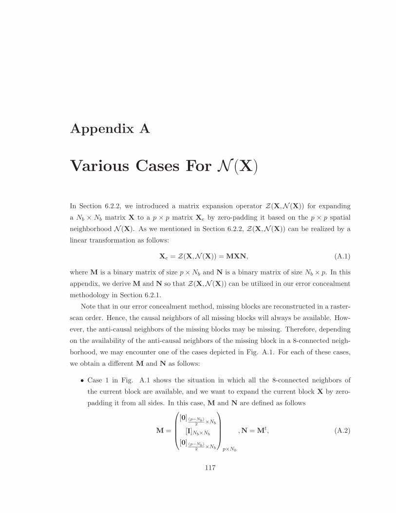
Appendix A
Various Cases For N (X)
In Section 6.2.2, we introduced a matrix expansion operator Z(X,N (X)) for expanding
a Nb × Nb matrix X to a p × p matrix Xe by zero-padding it based on the p × p spatial
neighborhood N (X). As we mentioned in Section 6.2.2, Z(X,N (X)) can be realized by a
linear transformation as follows:
Xe = Z(X,N (X)) = MXN, (A.1)
where M is a binary matrix of size p×Nb and N is a binary matrix of size Nb × p. In this
appendix, we derive M and N so that Z(X,N (X)) can be utilized in our error concealment
methodology in Section 6.2.1.
Note that in our error concealment method, missing blocks are reconstructed in a raster-
scan order. Hence, the causal neighbors of all missing blocks will always be available. How-
ever, the anti-causal neighbors of the missing blocks may be missing. Therefore, depending
on the availability of the anti-causal neighbors of the missing block in a 8-connected neigh-
borhood, we may encounter one of the cases depicted in Fig. A.1. For each of these cases,
we obtain a different M and N as follows:
• Case 1 in Fig. A.1 shows the situation in which all the 8-connected neighbors of
the current block are available, and we want to expand the current block X by zero-
padding it from all sides. In this case, M and N are defined as follows
M =
[0] (p−Nb)
2×Nb
[I]Nb×Nb
[0] (p−Nb)
2×Nb
p×Nb
,N = Mt, (A.2)
117

APPENDIX A. 118
Figure A.1: In the proposed error concealment method, depending on the availability of theneighbors of a missing block, various situations may arise. In this figure, the missing blockhas been depicted by a gray box while its available neighbors have been depicted by whiteboxes. The available neighbors of the missing block X are used to define N (X).
where [0]x×y denotes a x × y matrix whose elements are all zero, and [I]x×y denotes
the identity matrix of size x× y.
• Case 2 in Fig. A.1 shows the situation in which only the causal 8-connected neighbors
of the current block X are available, and we want to expand the current block by
zero-padding it from the top and left. In this case, M and N are defined as follows
M =
([0](p−Nb)×Nb
[I]Nb×Nb
)
p×Nb
,N = Mt. (A.3)
• Case 3 in Fig. A.1 shows the situation in which all the 8-connected neighbors of the
current block X are available except for one or more of its neighbors from below, and
we want to expand the current block by zero-padding it from the left, top, and right.
In this case, M and N are defined as follows
M =
([0](p−Nb)×Nb
[I]Nb×Nb
)
p×Nb
, (A.4)
N =([0]
Nb×(p−Nb)
2
[I]Nb×Nb[0]
Nb×(p−Nb)
2
)Nb×p
. (A.5)

APPENDIX A. 119
• Case 4 in Fig. A.1 shows the situation in which all 8-connected neighbors of the
current block are available except for one or more of its 8-connected neighbors to the
right, and we want to expand the current block X by zero-padding it from the left,
top, and bottom. In this case, M and N are defined as follows
M =
[0] (p−Nb)
2×Nb
[I]Nb×Nb
[0] (p−Nb)
2×Nb
p×Nb
, (A.6)
N =([0]Nb×(p−Nb) [I]Nb×Nb
)Nb×p
. (A.7)
• Case 5 in Fig. A.1 shows the situation in which the current block is on the left
boundary of the frame and all of its 8-connected neighbors are available, and we want
to expand the current block by zero-padding it from all sides except left. In this case,
M and N are defined as follows
M =
[0] (p−Nb)
2×Nb
[I]Nb×Nb
[0] (p−Nb)
2×Nb
p×Nb
, (A.8)
N =([I]Nb×Nb
[0]Nb×(p−Nb)
)Nb×p
. (A.9)
• Case 6 in Fig. A.1 shows the situation in which the current block is at the top-right
corner of the frame and all of its 8-connected neighbors are available, and we want to
expand the current block by zero-padding it from the left and bottom. In this case,
M and N are defined as follows
M =
([I]Nb×Nb
[0](p−Nb)×Nb
)
p×Nb
, (A.10)
N =([0]Nb×(p−Nb) [I]Nb×Nb
)Nb×p
. (A.11)

APPENDIX A. 120
• Case 7 in Fig. A.1 shows the situation in which the current block is at the top-left
corner of the frame and all of its 8-connected neighbors are available, and we want to
expand the current block by zero-padding it from the right and bottom. In this case,
M and N are defined as follows
M =
([I]Nb×Nb
[0](p−Nb)×Nb
)
p×Nb
, (A.12)
N =([I]Nb×Nb
[0]Nb×(p−Nb)
)Nb×p
. (A.13)
• Case 8 in Fig. A.1 shows the situation in which the current block is at the bottom-left
corner of the frame and all of its 8-connected neighbors are available, and we want to
expand the current block by zero-padding it from the top and right. In this case, M
and N are defined as follows
M =
([0](p−Nb)×Nb
[I]Nb×Nb
)
p×Nb
, (A.14)
N =([I]Nb×Nb
[0]Nb×(p−Nb)
)Nb×p
. (A.15)
• Case 9 in Fig. A.1 shows the situation in which the current block in on the top
boundary of the frame and all of its 8-connected neighbors are available, and we want
to expand the current block by zero-padding it from all sides except the top. In this
case, M and N are defined as follows
M =
([I]Nb×Nb
[0](p−Nb)×Nb
)
p×Nb
, (A.16)
N =([0]
Nb×(p−Nb)
2
[I]Nb×Nb[0]
Nb×(p−Nb)
2
)Nb×p
. (A.17)
For all other possible cases, we assume that N (X) covers only X, and so we set both M
and N to Nb ×Nb identity matrices.

Bibliography
[1] H. Hadizadeh, I. V. Bajic, and G. Cheung, “Saliency-cognizant error concealment
in loss-corrupted streaming video,” in Proc. IEEE Int. Conf. Multimedia Expo, July
2012, pp. 73–79.
[2] L. Itti, C. Koch, and E. Niebur, “A model of saliency-based visual attention for rapid
scene analysis,” IEEE Trans. Pattern Anal. Machine Intell., vol. 20, pp. 1254–1259,
Nov. 1998.
[3] L. Itti and C. Koch, “A saliency-based search mechanism for overt and covert shifts
of visual attention,” Vision Research, vol. 40, pp. 1489–1506, 2000.
[4] W. James, The Principles of Psychology. Holt, New York, 1890.
[5] L. Itti, “Automatic foveation for video compression using a neurobiological model of
visual attention,” IEEE Trans. Image Process., vol. 13, no. 10, pp. 1304–1318, 2004.
[6] A. Borji and L. Itti, “State-of-the-art in visual attention modeling,” IEEE Trans.
Pattern Anal. Mach. Intell., vol. 35, no. 1, p. 185207, Jan. 2013.
[7] J. M. Shapiro, “Embedded image coding using zerotrees of wavelet coefficients,” IEEE
Trans. Signal Process., vol. 41, pp. 3445–3462, Dec. 1993.
[8] P. T. Kortum and W. S. Geisler, “Implementation of a foveated image coding system
for image bandwidth reduction,” in Human Vision and Electronic Imaging, SPIE
Proceedings, 1996, pp. 350–360.
[9] N. Doulamis, A. Doulamis, D. Kalogera, and S. Kollias, “Improving the performance
of MPEG coders using adaptive regions of interest,” IEEE Trans. Circuits Syst. Video
Technol., vol. 8, pp. 928–934, 1998.
121

BIBLIOGRAPHY 122
[10] L. B. Stelmach, W. J. Tam, and P. J. Hearty, “Static and dynamic spatial resolu-
tion in image coding: An investigation of eye movements,” in Human Vision, Visual
Processing, and Digital Display II, SPIE Proceedings, 1991, pp. 147–152.
[11] M. Hannuksela, Y.-K. Wang, and M. Gabbouj, “Sub-picture: ROI coding and unequal
error protection,” Proc. IEEE Int. Conf. Image Process., vol. 3, pp. 537 – 540, 2002.
[12] H. Hadizadeh, M. J. Enriquez, and I. V. Bajic, “Eye-tracking database for a set of
standard video sequences,” IEEE Trans. Image Process., vol. 21, no. 2, pp. 898–903,
Feb. 2012.
[13] H. Hadizadeh, I. V. Bajic, and G. Cheung, “Video error concealment using a
computation-efficient low saliency prior,” submitted to IEEE Trans. Multimedia.
Available: http://mcl.ensc.sfu.ca/pubs/hbc-tmm-sub-2012.pdf, 2012.
[14] Y.-M. Chen and I. V. Bajic, “Motion vector outlier rejection cascade for global motion
estimation,” IEEE Signal Process. Lett., vol. 17, no. 2, pp. 197–200, Feb. 2010.
[15] H. Hadizadeh and I. V. Bajic, “Saliency-aware video compression,” submitted to IEEE
Trans. Image Process., Feb. 2013.
[16] ——, “Saliency-preserving video compression,” presented at IEEE Int. Conf. Multi-
media Expo (AVCC), Jul. 2011.
[17] L. Itti and P. F. Baldi, “A principled approach to detecting surprising events in video,”
in Proc. IEEE Conf. Comput. Vision Pattern Recog., San Siego, CA, Jun. 2005, pp.
631–637.
[18] M. Carrasco, “Visual attention: The past 25 years,” Vision Research, vol. 51, pp.
1484–1525, 2011.
[19] L. Itti, G. Rees, and J. K. Tsotsos, Neurobiology of Attention. Academic Press, 2005.
[20] J. R. Anderson, Cognitive psychology and its implications. Worth Publishers, 2004.
[21] S. Fuller, R. Z. Rodriguez, and M. Carrasco, “Apparent contrast differs across the
vertical meridian: Visual and attentional factors,” Journal of Vision, vol. 8, no. 1, pp.
11–16, 2008.

BIBLIOGRAPHY 123
[22] P. F. Montagna, B. and M. Carrasco, “Attention trades off spatial acuity,” Vision
Research, vol. 49, no. 7, pp. 735–745, 2009.
[23] L. Huang and K. R. Dobkins, “Attentional effects on contrast discrimination in hu-
mans: Evidence for both contrast gain and response gain,” Vision Research, vol. 45,
no. 9, pp. 1201–1212, 2005.
[24] J. Braun and B. Julesz, “Withdrawing attention at little or no cost: detection and
discrimination tasks,” Perception and Psychophysics, vol. 60, pp. 1–23, 1998.
[25] O. Hikosaka, S. Miyauchi, and S. Shimojo, “Orienting a spatial attention - its reflex-
ive, compensatory, and voluntary mechanisms,” Brain Research and Cognitive Brain
Research, vol. 5, pp. 1–9, 1996.
[26] J. R. Bergen and B. Julesz, “Parallel versus serial processing in rapid pattern discrim-
ination,” Nature, vol. 303, pp. 1176–1196, 1983.
[27] A. M. Sillito and H. E. Jones, “Context-dependent interactions and visual processing
in V1,” Journal of Physiology Paris, vol. 90, pp. 205–209, 1996.
[28] J. B. Levitt and J. S. Lund, “Context-dependent interactions and visual processing in
V1,” Nature, vol. 387, pp. 73–76, 1997.
[29] A. L. Yarbus, Eye-movements and Vision. Plenum Press, 1967.
[30] M. Sodhi, B. Reimer, J. L. Cohen, Vastenburg, R. Kaars, and S. Kirsschenbaum, “On-
road driver eye movement tracking using head-mounted devices,” Symp. Eye Tracking
Research and Applications, 2002.
[31] J. M. Henderson and A. Hollingworth, “High-level scene perception,” Ann. Rev. Psy-
chology, vol. 50, pp. 243–271, 1999.
[32] M. Land and M. Hayhoe, “In what ways do eye movements contribute to everyday
activities,” Vision Research, vol. 41, pp. 3559–3565, 2001.
[33] J. Shi and C. Tomasi, “Good features to track,” Proc. IEEE Conf. Computer Vision
Pattern Recog., pp. 593–600, 1994.
[34] B. Triggs, “Detecting keypoints with stable position, orientation, and scale under
illumination changes,” Proc. ECCV, pp. 100–113, 2004.

BIBLIOGRAPHY 124
[35] K. Yamada and G. W. Cottrell, “A model of scan paths applied to face recognition,”
Proceedings of the Seventeenth Annual Cognitive Science Conference, pp. 55–60, 1995.
[36] N. Sebe and M. S. Lew, “Comparing salient point detectors,” Pattern Recognition
Letters, vol. 24, pp. 89–96, Jan. 2003.
[37] T. Kadir and M. Brady, “Scale, saliency and image description,” International Journal
of Computer Vision, vol. 45, pp. 83–105, 2001.
[38] J. Harel, C. Koch, and P. Perona, “Graph-based visual saliency,” in Proc. NIPS, 2006,
pp. 313–335.
[39] V. Navalpakkam and L. Itti, “An integrated model of top-down and bottom-up atten-
tion for optimal object detection,” Proc. IEEE Computer Vision Pattern Recog., pp.
2049–2056, 2006.
[40] E. Borenstein and S. Ullman, “Learn to segment,” Proc. European Conference on
Computer Vision, pp. 315–328, 2004.
[41] P. Felzenszwalb, R. Girshick, D. McAllester, and D. Ramanan, “Object detection
with discriminatively trained part based models,” IEEE Trans. Pattern Anal. Mach.
Intell., no. 9, 2010.
[42] P. Viola and M. J. Jones, “Robust real-time face detection,” International Journal of
Computer Vision, no. 2, 2004.
[43] V. Navalpakkam and L. Itti, “Search goal tunes visual features optimally,” Neuron,
vol. 53, no. 4, pp. 605–617, 2007.
[44] A. M. Treisman and G. Gelade, “A feature integration theory of attention,” Cognitive
Psychology, vol. 12, pp. 97–136, 1980.
[45] C. Koch and S. Ullman, “Shifts in selective visual attention:towards the underlying
neural circuitry,” Human Neurobiology, vol. 4, pp. 219–227, 1985.
[46] J. K. Tsotsos, S. M. Culhane, W. Y. K. Wai, Y. Lai, N. Davis, and F. Nuflo, “Modeling
visual attention via selective tuning,” Artificial Intelligence, vol. 78, pp. 507–545, 1995.
[47] S. Baluja and D. Pomerleau, “Using a saliency map for active spatial selective atten-
tion:implementation and initial results,” Proc. NIPS, pp. 451–458, 1994.
BIBLIOGRAPHY 125
[48] C. Guo and L. Zhang, “A novel multiresolution spatiotemporal saliency detection
model and its applications in image and video compression,” IEEE Trans. Image
Process., vol. 19, no. 1, pp. 185–198, Jan. 2010.
[49] O. Le Meur and P. Le Callet, “What we see is most likely to be what matters : visual
attention and applications,” Proc. IEEE Int. Conf. Image Process., pp. 3085–3088,
2009.
[50] S. Marat, T. Ho Phuoc, L. Granjon, N. Guyader, D. Pellerin, and A. Gurin-Dugu,
“Spatio-temporal saliency model to predict eye movements in video free viewing,”
Proc. 16th European Signal Process. Conf. (EUSIPCO’08), 2008.
[51] Y. Zhai and M. Shah, “Visual attention detection in video sequences using spatiotem-
poral cues,” Proc. ACM Int. Conf. Multimedia, 2006.
[52] O. Boiman and M. Irani, “Detecting irregularities in images and in video,” Proc. IEEE
Int. Conf. Computer Vision, 2005.
[53] N. d. B. Bruce and J. K. Tsotsos, “Saliency based on information maximization,”
Proc. Advances in Neural Info. Proc. Systems, 2005.
[54] R. Desimone and J. Duncan, “Neural mechanisms of selective visual attention,” Ann.
Rev. Neuroscience, vol. 18, pp. 193–222, 1995.
[55] O. Le Meur, P. Le Callet, and D. Barba, “Predicting visual fixations on video based
on low-level visual features,” Vision Research, vol. 47, no. 19, pp. 2483–2498, Sep.
2007.
[56] B. A. Wandell, Foundations of Vision. Sinauer Associates, 1995.
[57] L. Itti and P. F. Baldi, “Bayesian surprise attracts human attention,” in Advances in
Neural Inf. Process. Syst. MIT Press, 2006, pp. 547–554.
[58] ——, “Bayesian surprise attracts human attention,” Vision Research, vol. 49, no. 10,
pp. 1295–1306, May 2009.
[59] A. Oliva, A. Torralba, M. S. Castelhano, and J. M. Henderson, “Top-down control of
visual attention in object detection,” Proc. Int. Conf. Image Process., pp. 253–256,
2003.

BIBLIOGRAPHY 126
[60] L. Zhang, M. H. Tong, T. K. Marks, H. Shan, and G. W. Cottrell, “SUN: a bayesian
framework for saliency using natural statistics,” Journal of Vision, vol. 8, no. 32, pp.
1–20, 2008.
[61] A. Torralba, “Modeling global scene factors in attention,” Journal of the Optical
Society of America, vol. 20, pp. 1407–1418, 2003.
[62] T. M. Cover and J. A. Thomas, Elements of Information Theory. John Wiley and
Sons, 1991.
[63] D. Gao and N. Vasconcelos, “Discriminant saliency, the detection of suspicious coin-
cidences, and applications to visual recognition,” IEEE Trans. Pattern Anal. Mach.
Intell., vol. 31, no. 6, pp. 989–1005, Jun. 2009.
[64] C. Bishop, Pattern Recognition and Machine Learning. Springer, 2006.
[65] X. Hou and L. Zhang, “Saliency detection: A spectral residual approach,” Proc. IEEE
Int. Conf. Computer Vision Pattern Recog., 2007.
[66] W. Kienzle, M. O. Franz, B. Scholkopf, and F. A. Wichmann, “Center-surround pat-
terns emerge as optimal predictors for human saccade targets,” Journal of Vision,
vol. 9, p. 115, 2009.
[67] L. Itti, “Automatic foveation for video compression using a neurobiological model of
visual attention,” IEEE Trans. Image Process., vol. 13, no. 10, pp. 1304–1318, 2004.
[68] N. D. B. Bruce and J. K. Tsotsos, “Saliency based on information maximization,”
Proc. NIPS, pp. 155–162, Jun. 2006.
[69] T. Judd, K. Ehinger, F. Durand, and A. Torralba, “Learning to predict where humans
look,” in Proc. IEEE ICCV, 2009.
[70] M. Cerf, J. Harel, W. Einhauser, and C. Koch, “Predicting human gaze using low-level
saliency combined with face detection,” Proc. NIPS, vol. 20, pp. 241–248, 2007.
[71] R. J. Peters and L. Itti, “Beyond bottom-up: Incorporating task dependent influences
into a computational model of spatial attention,” Proc. IEEE Conf. Computer Vision
Pattern Recog., 2007.
BIBLIOGRAPHY 127
[72] Z. Li, S. Qin, and L. Itti, “Visual attention guided bit allocation in video compression,”
Image and Vision Computing, vol. 29, pp. 1 –14, 2011.
[73] J. Li, Y. Tian, T. Huang, and W. Gao, “Probabilistic multi-task learning for visual
saliency estimation in video,” Int. Journal of Computer Vision, vol. 90, pp. 150–165,
2010.
[74] F. Shic and B. Scassellati, “A behavioral analysis of computational models of visual
attention,” Int. Journal of Computer Vision, vol. 73, pp. 159–177, 2007.
[75] P. K. Mital, T. J. Smith, R. L. Hill, and J. M. Henderson, “Clustering of gaze during
dynamic scene viewing is predicted by motion,” Cognitive Computation, vol. 3, no. 1,
pp. 5–24, Mar. 2011.
[76] “Stefan Winkler’s website,” http://stefan.winkler.net/.
[77] “Locarna systems,” http://www.locarna.com.
[78] J. T. McClave and T. Sincich, Statistics. Prentice Hall, Upper Saddle River, NJ, 9th
edition, 2003.
[79] ITU-R, “Recommendation BT.500-8: Methodology for the subjective assessment of
the quality of television pictures,” International Telecommunications Union, Tech.
Rep., 1998.
[80] M. Cerf, E. P. Frady, and C. Koch, “Faces and text attract gaze independent of the
task: Experimental data and computer model,” Vision Research, vol. 9(12), no. 10,
pp. 1–15, 2009.
[81] B. Tatler, R. Baddeley, and I. Gilchrist, “Visual correlates of fixation selection: Effects
of scale and time,” Vision Research, vol. 45, no. 5, pp. 643–659, 2005.
[82] “Saliency benchmark datasets,” [Online] Available:
http://people.csail.mit.edu/tjudd/SaliencyBenchmark/.
[83] S. Lee, M. S. Pattichis, and A. C. Bovik, “Foveated video quality assessment,” IEEE
Trans. Multimedia, vol. 4, pp. 129–132, Mar. 2002.

BIBLIOGRAPHY 128
[84] Y. Fang, Z. Chen, W. Lin, and C.-W. Lin, “Saliency detection in the compressed
domain for adaptive image retargeting,” IEEE Trans. Image Process., vol. 21, no. 9,
pp. 3888–3901, Sep. 2012.
[85] R. Achanta, S. Hemami, F. Estrada, and S. Susstrunk, “Frequency-tuned salient region
detection,” in Proc. IEEE Comput. Vision Pattern Recog., Miami Beach, FL, June
2009.
[86] J. W. Woods,Multidimensional signal, image, and video processing and coding, 2nd ed.
Academic Press/Elsevier, 2012.
[87] H. Stark and J. W. Woods, Probability, statistics, and random processes for engineers,
4th ed. Pearson/Prentice Hall, 2012.
[88] J. S. Lim, Two-dimensional signal and image processing. Prentice Hall, 1989.
[89] A. Torralba and A. Oliva, “Statistics of natural image categories,” Network: Comput.
Neural Syst., vol. 14, pp. 391–412, 2003.
[90] L. Itti, “Quantifying the contribution of low-level saliency to human eye movements
in dynamic scenes,” Visual Cognition, vol. 12, no. 6, pp. 1093–1123, 2005.
[91] Z. Wang and Q. Li, “Video quality assessment using a statistical model of human
visual speed perception,” Journal of the Optical Society of America, vol. 24, no. 2, pp.
B61–B69, Dec. 2007.
[92] V. A. Mateescu, H. Hadizadeh, and I. V. Bajic, “Evaluation of several visual saliency
models in terms of gaze prediction accuracy on video,” in Proc. IEEE Globecom’12
Workshop: QoEMC, Dec. 2012.
[93] Y. Fang, Z. Chen, W. Lin, and C.-W. Lin, “Saliency detection in the compressed
domain for adaptive image retargeting,” IEEE Trans. Image Process., vol. 9, no. 21,
pp. 3888–3901, Sep. 2012.
[94] C. Chamaret, J. C. Chevet, and O. Le Meur, “Spatio-temporal combination of saliency
maps and eye-tracking assessment of different strategies,” IEEE International Conf.
on Image Proc., pp. 1077–1080, Sep. 2010.

BIBLIOGRAPHY 129
[95] D. J. Sheskin, Handbook of Parametric and Nonparametric Statistical Procedures.
Chapman & Hall/CRC, 2007.
[96] “iLab neuromorphic vision C++ toolkit,” [Online] Available:
http://ilab.usc.edu/toolkit/.
[97] B. Schauerte and R. Stiefelhagen, “Predicting human gaze using quaternion DCT
image signature saliency and face detection,” Proc. IEEE WACV’12, pp. 137–144,
2012.
[98] S. Goferman, L. Zelnik-Manor, and A. Tal, “Context-aware saliency detection,” Proc.
IEEE Computer Vision Pattern Recog., pp. 2376–2383, Jun. 2010.
[99] Y. Fang, W. Lin, B. Lee, C. Lau, Z. Chen, and C. Lin, “Saliency detection model
based on human visual sensitivity and amplitude spectrum,” IEEE Trans. Multimedia,
vol. 14, no. 1, pp. 187–198, Feb. 2012.
[100] H. J. Seo and P. Milanfar, “Static and space-time visual saliency detection by self-
resemblance,” Journal of Vision, vol. 9, no. 12, pp. 1–27, Nov. 2009.
[101] W. Kim, C. Jung, and C. Kim, “Spatiotemporal saliency detection and its applications
in static and dynamic scenes,” IEEE Trans. Circuits Syst. Video Technol., vol. 21,
no. 4, pp. 446–456, Apr. 2011.
[102] Y. Hochberg and A. C. Tamhane, Multiple Comparison Procedures. Hoboken, NJ:
John Wiley and Sons, 1987.
[103] H. Hadizadeh, I. V. Bajic, and G. Cheung, “Complexity of saliency-cognizant er-
ror concealment based on the Itti-Koch-Niebur saliency model,” [Online] Available:
http://summit.sfu.ca/item/10942, Multimedia Communications Lab, Simon Fraser
University, Tech. Rep. MCL-TR-2012-11-01, Nov. 2012.
[104] A. Smolic, M. Hoeynck, and J.-R. Ohm, “Low-complexity global motion estimation
from P-frame motion vectors for MPEG-7 applications,” in Proc. IEEE Int. Conf.
Image Process., vol. 2, Sep. 2000, pp. 271–274.
[105] G. H. Golub and C. F. Van Loan, Matrix Computations. Mathematics, 1996.

BIBLIOGRAPHY 130
[106] M. A. Robertson and R. L. Stevenson, “DCT quantization noise in compressed im-
ages,” IEEE Trans. Circuits Syst. for Video Technol., vol. 15, no. 1, pp. 27–38, 2005.
[107] A. Leontaris, P. C. Cosman, and A. R. Reibman, “Quality evaluation of motion-
compensated edge artifacts in compressed video,” IEEE Trans. Image Process., vol. 16,
no. 11, pp. 943–956, Apr. 2007.
[108] Z. Chen, N. K. Ngan, and W. Lin, “Perceptual video coding: Challenges and ap-
proaches,” in Proc. IEEE Int. Conf. Multimedia Expo, Jul. 2010, pp. 784–789.
[109] Y. Liu, Z. Li, and Y. C. Soh, “Region-of-interest based resource allocation for con-
versational video communications of H.264/AVC,” IEEE Trans. Circuits and Syst.
Video Technol., vol. 18, no. 1, pp. 134 –139, 2008.
[110] S. Daly, “The visible difference predictor: an algorithm for the assessment of image
fidelity,” in Digital Images and Human Vision, A. B. Watson, Ed. MIT Press, 1993,
pp. 179–206.
[111] I. E. Richardson, The H.264 Advanced Video Compression Standard. Wiley, 2010.
[112] T. Wiegand and B. Girod, “Lagrange multiplier selection in hybrid video coder con-
trol,” Proc. IEEE Int. Conf. Image Process., vol. 3, pp. 542–545, 2001.
[113] G. Sullivan and T. Wiegand, “Rate-distortion optimization for video compression,”
IEEE Signal Process. Mag., vol. 15, no. 6, pp. 74–90, 1998.
[114] “The H.264/AVC JM reference software,” [Online] Available:
http://iphome.hhi.de/suehring/tml/.
[115] X. Li, N. Oertel, A. Hutter, and A. Kaup, “Laplace distribution based lagrangian rate
distortion optimization for hybrid video coding,” IEEE Trans. Circuits Syst. Video
Technol., vol. 19, no. 2, pp. 193–205, Feb. 2009.
[116] ——, “Advanced lagrange multiplier selection for hybrid video coding,” in Proc. IEEE
Conf. Multimedia Expo, July 2007, pp. 364–367.
[117] L. Chen and I. Garbacea, “Adaptive lambda estimation in Lagrangian rate-distortion
optimization for video coding,” in Visual Commun. Image Process. (VCIP), Jan. 2006.

BIBLIOGRAPHY 131
[118] J. Zhang, X. Yi, N. Ling, and W. Shang, “Context adaptive Lagrange multiplier
(CALM) for rate-distortion optimal motion estimation in video coding,” IEEE Trans.
Circuits Syst. Video Technol., vol. 20, no. 6, pp. 820–828, June 2010.
[119] M. Jiang and N. Ling, “On Lagrange multiplier and quantizer adjustment for H.264
frame-layer video rate control,” IEEE Trans. Circuits Syst. Video Technol., vol. 16,
no. 5, pp. 663–669, May 2006.
[120] M. Wang and B. Yan, “Lagrangian multiplier based joint three-layer rate control for
H.264/AVC,” IEEE Signal Process. Lett., vol. 16, no. 8, pp. 679–682, Aug. 2009.
[121] X. Yang, W. Lin, Z. Lu, E. Ong, and S. Yao, “Motion-compensated residue pre-
processing in video coding based on just-noticeable distortion profile,” IEEE Trans.
Circuits Syst. Video Technol., vol. 15, no. 6, pp. 742–752, Jun. 2005.
[122] Z. Chen and C. Guillemot, “Perceptually-friendly H.264/AVC video coding based
on foveated just-noticeable-distortion model,” in IEEE Trans. Circuits Syst. Video
Technol., vol. 20, no.6, June 2010, pp. 806–819.
[123] W. S. Geisler and J. S. Perry, “A real-time foveated multiresolution system for low-
bandwidth video communication,” Proc. SPIE, vol. 3299, pp. 294–305, Jul. 1996.
[124] Z. Wang and A. C. Bovik, “Embedded foveation image coding,” IEEE Trans. Image
Proc., vol. 10, pp. 1397–1410, Oct. 2001.
[125] Z. Wang, L. Lu, and A. C. Bovik, “Foveation scalable video coding with automatic
fixation selection,” IEEE Trans. Image Proc., vol. 12, no. 2, pp. 1–12, Feb. 2003.
[126] Z. Wang, A. C. Bovik, H. R. Sheikh, and E. P. Simoncelli, “Image quality assessment:
From error visibility to structural similarity,” IEEE Trans. Image Process., vol. 13,
no. 4, pp. 600–612, Apr. 2004.
[127] C. Yang, R. Leung, L. Po, and Z. Mai, “An SSIM-optimal H.264/AVC inter frame
encoder,” Proc. IEEE International Conference on Intelligent Computing and Intelli-
gent Systems, vol. 4, pp. 291–295, 2009.
[128] C. Yang, H. Wang, and L. Po, “Improved inter prediction based on structural sim-
ilarity in H.264,,” Proc. IEEE International Conference on Signal Processing and
Communications, vol. 2, pp. 340–343, 2007.
BIBLIOGRAPHY 132
[129] Y. H. Huang, T. S. Ou, P. Y. Su, and H. Chen, “Perceptual rate-distortion optimiza-
tion using structural similarity index as quality metric,” IEEE Trans. Circuits Syst.
Video Technol., vol. 20, no. 11, pp. 1614–1624, Nov. 2010.
[130] S. Wang, A. Rehman, Z. Wang, S. Ma, and W. Gao, “SSIM-motivated rate-distortion
optimization for video coding,” IEEE Trans. Circuits Syst. Video Technol., vol. 22,
no. 4, pp. 516–529, Apr. 2012.
[131] X. Wang, L. Su, Q. Huang, and C. Liu, “Visual perception based Lagrangian rate
distortion optimization for video coding,” Proc. IEEE Int. Conf. on Image Process.,
vol. 20, pp. 1653 – 1656, Sep. 2011.
[132] Z. G. Li, W. Gao, F. Pan, S. W. Ma, K. P. Lim, G. N. Feng, X. Lin, S. Rahardja,
H. Q. Lu, and Y. Lu, “Adaptive rate control for H.264,” J. Visual Commun. Image
Represent., vol. 17, pp. 376–406, Apr. 2006.
[133] N. Kamaci, Y. Altunbasak, and R. M. Mersereau, “Frame bit allocation for the
H.264/AVC video coder via Cauchy-density-based rate and distortion models,” IEEE
Trans. Circuits Syst. Video Technol., vol. 15, no. 8, pp. 994–1006, Aug. 2005.
[134] Z. Chen and K. N. Ngan, “Toward rate-distortion tradeoff in real-time color video
coding,” IEEE Trans. Circuits Syst. Video Technol., vol. 17, no. 2, pp. 158–167, Feb.
2007.
[135] C. Yeo, Y. Han Tan, Z. Li, and S. Rahardja, “Mode-dependent transforms for coding
directional intra prediction residuals,” Electronics Letters, vol. 22, no. 4, pp. 545–554,
Apr. 2012.
[136] A. K. Jain, Fundamentals of Digital Image Processing. NJ: Prentice-Hall, 1989.
[137] I.-M. Pao and M.-T. Sun, “Modeling DCT coefficients for fast video encoding,” IEEE
Trans. Circuits Syst. Video Technol., vol. 9, no. 4, pp. 608–616, Jun. 1999.
[138] B. Widrow and I. Kollar, Quantization Noise. Cambridge, 2008.
[139] G. Bjontegaard, “Calculation of average PSNR differences between RD curves
(VCEG-M33),” VCEG Meeting (ITU-T SG16 Q.6), Apr. 2001.

BIBLIOGRAPHY 133
[140] M. Pinson and S. Wolf, “A new standardized method for objectively measuring video
quality,” IEEE Trans. Broadcasting, vol. 50, no. 3, pp. 312–322, June 2004.
[141] S. Chikkerur, V. Sundaram, M. Reisslein, and L. J. Karam, “Objective video quality
assessment methods: A classification, review, and performance comparison,” IEEE
Trans. Broadcasting, vol. 57, no. 2, pp. 165–182, June 2011.
[142] M. Taylor and C. Creelman, “PEST: Efficient estimates on probability functions,”
Journal of Acoustical Society of America, vol. 41, pp. 782–787, 1967.
[143] ITU-R, “Recommendation BT.500-8: Methodology for the subjective assessment of
the quality of television pictures,” ITU, Tech. Rep., 1998.
[144] D. J. Sheskin, Handbook of Parametric and Nonparametric Statistical Procedures.
Chapman & Hall/CRC, 2007.
[145] “Cisco visual networking index: Forecast and methodology 2010-2015,”
http://www.cisco.com/.
[146] A. Kubota, A. Smolic, M. Magnor, M. Tanimoto, T. Chen, and C. Zhang, “Multi-view
imaging and 3DTV,” in IEEE Signal Process. Mag., vol. 24, no.6, Nov. 2007.
[147] G.-M. Muntean, G. Ghinea, and T. Sheehan, “Region of interest-based adaptive mul-
timedia streaming scheme,” in IEEE Trans. Broadcast., vol. 54, no.2, June 2008, pp.
296–303.
[148] F. Boulos, W. Chen, B. Parrein, and P. L. Callet, “A new H.264/AVC error resilience
model based on regions of interest,” in Proc. 17th International Packet Video Work-
shop (PV 2009), Seattle, WA, May 2009.
[149] N. Bruce and P. Kornprobst, “Region-of-interest intra prediction for H.264/AVC error
resilience,” in Proc. IEEE Int. Conf. Image Process., Cairo, Egypt, Nov. 2009.
[150] Y. Chen, Y. Hu, O. Au, H. Li, and C. W. Chen, “Video error concealment using
spatio-temporal boundary matching and partial differential equation,” in IEEE Trans.
Multimedia, vol. 10, no.1, Jan. 2008, pp. 2–15.
[151] “Oxford dictionary: definition of concealment,” [Online] Available:
http://oxforddictionaries.com/definition/american english/conceal.

BIBLIOGRAPHY 134
[152] C. Yeo, W.-T. Tan, and D. Mukherjee, “Receiver error concealment using acknowledge
preview (RECAP)–an approach to resilient video streaming,” in Proc. IEEE Int. Conf.
Acoustics, Speech and Signal Process., Taipei, Taiwan, Apr. 2009.
[153] I. V. Bajic, “Error control for broadcasting and multicasting: An overview,” in Mo-
bile Multimedia Broadcasting Standards: Technology and Practice, F.-L. Luo, Ed.
Springer, 2008, pp. 313–335.
[154] E. Maani and A. K. Katsaggelos, “Unequal error protection for robust streaming
of scalable video over packet lossy networks,” IEEE Trans. Circ. Syst. Video Tech.,
vol. 20, no. 3, pp. 407–416, Mar. 2010.
[155] I. E. G. Richardson, H.264 and MPEG-4 Video Compression: Video Coding for Next-
Generation Multimedia. NJ:Wiley, 2003.
[156] H. Hadizadeh and I. V. Bajic, “Burst loss resilient packetization of video,” IEEE
Trans. Image Process., 2011.
[157] X. Hou and L. Zhang, “Saliency detection: A spectral residual approach,” in Proc.
IEEE Comput. Vision Pattern Recog., Minneapolis, MN, June 2007.
[158] P. List, A. Joch, J. Lainema, G. Bjntegaard, and M. Karczewicz, “Adaptive deblocking
filter,” IEEE Trans. Circuits Syst. Video Technol., vol. 13, no. 7, pp. 614–619, July
2003.
[159] P. P. Vaidyanathan, Multirate Systems and Filter Banks. Prentice-Hall, 1993.
[160] Y. Nesterov and A. Nemirovskii, Interior-Point Polynomial Algorithms in Convex
Programming. Siam Studies in Applied Mathematics, 1994.
[161] S. Boyd and L. Vandenberghe, Convex Optimization. Cambridge University Press,
2004.
[162] J. R. Magnus and H. Neudecker, Matrix Differential Calculus with Applications in
Statistics and Econometrics. Wiley, 1999.
[163] “cvx users guide,” [online] http://cvxr.com/cvx/.
[164] R. W. Vuduc, “Automatic performance tuning of sparse matrix kernels,” Ph.D. dis-
sertation, Computer Science, University of California, Berkeley, Fall 2003.

BIBLIOGRAPHY 135
[165] E. N. Gilbert, “Capacity of a burst-noise channel,” Bell Sys. Tech. J., vol. 39, pp.
1253–1266, Sep. 1960.
[166] S. H. Khatoonabadi and I. V. Bajic, “Video object tracking in the compressed domain
using spatio-temporal Markov random fields,” IEEE Trans. Image Process., vol. 22,
no. 1, pp. 300 – 313, Jan. 2013.
[167] A. Hagiwara, A. Sugimoto, and K. Kawamoto, “Saliency-based image editing for guid-
ing visual attention,” in Proc. 1st International Workshop on Pervasive Eye Tracking
and Mobile Eye-Based Interaction, Beijing, China, Sep. 2011.
Recommended

![Bahman Bahmani bahman@stanford.edu. Fundamental Tradeoffs Drug Interaction Example [Adapted from Ullman’s slides, 2012] Technique I: Grouping](https://img.pdfslide.us/doc/110x75/56649ca75503460f94969a01/bahman-bahmani-bahmanstanfordedu-fundamental-tradeoffs-drug-interaction.jpg)