i
Use of remote sensing in landscape-scale vegetation degradation assessment in the semi-
arid areas of the Save catchment, Zimbabwe
__________________________________
By
Dadirai Matarira
Student Number: 217081922
Submitted in fulfilment of the requirements for the degree of Master of Science in Environmental
Sciences
School of Agricultural, Earth and Environmental Sciences
University of KwaZulu-Natal, South Africa
2019
Supervisor: Professor O. Mutanga
Co- Supervisor: Professor T. Dube

ii
Abstract
The deteriorating condition of land in parts of the world is negatively affecting livelihoods,
especially, in rural communities of the developing world. Zimbabwe has experienced significant
vegetation cover losses, particularly, in low and varied rainfall areas of the Save catchment. The
concern that Save catchment is undergoing huge vegetation losses has been largely expressed,
with the causes being environmental and anthropogenic. Given the magnitude of the problem,
research studies have been undertaken to assess the extent of the problem in the south eastern
region of Zimbabwe, which, nevertheless, have been mainly localized. The present study seeks
to identify and quantify vegetation degradation at a landscape scale in the Save catchment of
Zimbabwe, using remote sensing technologies. To achieve this, two objectives were set. The first
objective provided a review of the application of satellite earth observations in assessing
vegetation degradation, the causes, as well as associated impacts at different geographical scales.
A review of literature has revealed the effectiveness of satellite information in identifying
changes in vegetation condition. A second objective sought to establish the extent of vegetation
degradation in the Save catchment. Moderate Resolution Imaging Spectroradiometer-
Normalised Difference Vegetation Index (MODIS NDVI) datasets were used for mapping NDVI
trends over the period 2000-2015. Further analysis involved application of residual trend
(RESTREND) method to separate human influences from climatic signal on vegetation
degradation. RESTREND results showed an increasing trend in NDVI values in about 33.6% of
the Save catchment and a decreasing trend in about 18.3% from 2000 to 2015. The results of the
study revealed that about 3,609,955 hectares experienced significant human induced vegetation
degradation. Approximately 38.8% of the Save Catchment was significantly degraded (p< 0.05),
3.6%, 12.8%, and 22.4% of which were classified as severely, moderately, and lightly degraded,
respectively. Severe degradation was mainly found in the central districts of the Save Catchment,
mainly Bikita, Chipinge and northern Chiredzi. The results of this study support earlier reports
about ongoing degradation in the catchment. Vegetation changes observed across the landscape
revealed different degrees of the impacts of land use activities in altering the terrestrial
ecosystems. The study demonstrated the usefulness of the RESTREND method in identifying
vegetation loss due to human actions in very low rainfall areas.
Keywords: remote sensing; residual trend; NDVI; semi-arid; vegetation degradation

iii
Preface
This research was undertaken at the School of Agricultural, Earth and Environmental Sciences,
University of KwaZulu-Natal, Pietermaritzburg, South Africa, under the supervision of Professor
Onisimo Mutanga and Professor Timothy Dube.
I declare that the work presented in this thesis has never been submitted in any form to any other
institution. This work represents my original work except where due acknowledgements are
made.
Dadirai Matarira Signed … ……………… Date…………………….
As the candidate’s supervisor, I certify the above-mentioned statement and therefore approve this
thesis for submission.
Prof. Onisimo Mutanga Signed………………. Date………………………...
Prof. Timothy Dube Signed… ……… Date………………………

iv
Declaration
I, Dadirai Matarira, declare that:
1. The research reported in this thesis, except where otherwise indicated, is my original research.
2. This thesis has not been submitted for any degree or examination at any other institution.
3. This thesis does not contain other person’s data, pictures, graphs or other information, unless
specifically acknowledged as being sourced from other persons.
4. This thesis does not contain other persons’ writing, unless specifically acknowledged as being
sourced from other researchers. Where other written sources have been quoted:
a. Their words have been re-written and the general information attributed to them has
been referenced.
b. Where their exact words have been used, their writing has been placed in italics inside
quotation marks and referenced.
5. This thesis does not contain text, graphics or tables copied and pasted from the internet, unless
specifically acknowledged, and the source being detailed in the thesis and in the references
section.
Signed… …………………… Date……………………….

v
Dedication
I dedicate this dissertation to my husband, Caxton, and my children, Tavonga and Tadiwa, for
their tremendous support. To God be the glory.

vi
Acknowledgements
Firstly, I would like to thank the Lord, Almighty, for giving me the strength to pursue this
programme.
My sincere appreciation goes to my supervisor, Professor Onisimo Mutanga and co-supervisor,
Professor Timothy Dube, for guiding me throughout the research process, from proposal
development, to the submission of the thesis. Their advice and invaluable feedback on my
submissions made it possible for me to achieve my goal.
I would also want to acknowledge the following people for their contributions: Sharon Chawanji,
Dr Mbulisi Sibanda, Mr Trylee Matongera and Hardlife Muhoyi. I am very grateful for their
research support.
My research would not have been possible without the support of my husband, Caxton and my
beloved children, Tavonga and Tadiwa. I would like to thank them for their encouragement.
To Josephine Hapazari and family, thank you very much for your support.

vii
Table of Contents
Abstract ......................................................................................................................................... ii
Preface ........................................................................................................................................... iii
Declaration.................................................................................................................................... iv
Acknowledgements ...................................................................................................................... vi
CHAPTER 1 .................................................................................................................................. 1
General Introduction .................................................................................................................... 1
1.1 Introduction ....................................................................................................................................... 1
1.2 Aim & Objectives .............................................................................................................................. 3
1.3 Research questions ............................................................................................................................ 4
1.4 General structure of the thesis ......................................................................................................... 4
CHAPTER TWO .......................................................................................................................... 5
Progress in remote sensing applications in vegetation degradation assessment and
monitoring in sub-Saharan Africa .............................................................................................. 5
Abstract .................................................................................................................................................... 5
2.1 Introduction ....................................................................................................................................... 6
2.2 Degradation on a global scale .......................................................................................................... 8
2.3 Drivers of vegetation degradation ................................................................................................. 10
2.4 Cost of vegetation degradation ...................................................................................................... 11
2.5 Biophysical manifestation of vegetation degradation .................................................................. 13
2.6 Remote sensing and application of NDVI in vegetation degradation assessment ..................... 14
2.6.1. Relevance of NDVI in vegetation degradation assessment .................................................... 16
2.6.2 Limitations of NDVI in vegetation degradation assessment ................................................... 17
2.7 Differentiating the climate- and human-induced drivers of vegetation degradation by
RESTREND method ............................................................................................................................. 18
2.8 Conclusions ...................................................................................................................................... 19
CHAPTER THREE .................................................................................................................... 20
Landscape scale vegetation degradation mapping in the semi- arid areas of the Save
catchment, Zimbabwe................................................................................................................. 20
Abstract .................................................................................................................................................. 20
3.1 Introduction ..................................................................................................................................... 21
3.2 Materials and methods ................................................................................................................... 23

viii
3.2.1 Description of the study area .................................................................................................... 23
3.2.2 Rainfall data processing ........................................................................................................... 24
3.2.3 MODIS NDVI data acquisition and processing....................................................................... 25
3.2.4 Data analysis ............................................................................................................................. 25
3.2.5 Raw NDVI trend analysis ......................................................................................................... 25
3.2.6 Residual trend analysis method ................................................................................................ 26
3.3 Results .............................................................................................................................................. 28
3.3.1 NDVI linear trends in the Save catchment .............................................................................. 28
3.3.2 Spatial patterns of the NDVI – rainfall relationship ............................................................... 31
3.3.3 Spatial patterns of the NDVI residual trends ........................................................................... 35
3.3.4 Comparison of RESTREND with raw vegetation index trends ............................................... 37
3.3.5 Severity of vegetation degradation ............................................................................................ 37
3.4 Discussion......................................................................................................................................... 39
3.5 Conclusions ...................................................................................................................................... 44
CHAPTER FOUR: Objectives reviewed and conclusions ...................................................... 45
4.1 Introduction ........................................................................................................................... 45
4.2 Objectives reviewed ........................................................................................................................ 45
4.3 Conclusions ...................................................................................................................................... 47

ix
List of figures
Figure 3.1 Study area- Save catchment area in Zimbabwe ........................................................... 24
Figure 3. 2 NDVI trends in the Save Catchment where A. is a rate of change in normalised
difference vegetation index (NDVI) as a function of time (year) in the Save catchment of
Zimbabwe and B. shows significant NDVI trends (p<0.05) ........................................................ 29
Figure 3. 3 Rate of change in normalised difference vegetation index (NDVI) as a function of
rainfall in the Save catchment of Zimbabwe ................................................................................ 31
Figure 3. 4 Coefficient of determination (R2) of NDVI –rainfall relationship ............................. 32
Figure 3. 5 Regressions between NDVImax and rainfall for (a) Marondera (grid point18.5S, 32E),
(b) Chimanimani (grid point 20S, 32.75E), (c) Chiredzi (grid point 22S, 31.5E) and (d) Buhera
(grid point 19.5S, 32E).................................................................................................................. 33
Figure 3. 6 Intercept of the relationship between NDVI and rainfall in the Save catchment of
Zimbabwe ..................................................................................................................................... 35
Figure 3. 7 Slope, which is the rate of change in normalised difference vegetation index (NDVI)
residuals as function of time (2000-2015), in the Save catchment of Zimbabwe......................... 35
Figure 3. 8 Areas showing significant negative residual trends at 95% significance level ......... 38

x
List of tables
Table 3. 1 Spatial distribution of normalised difference vegetation index (NDVI) change trend. 30
Table 3. 2. Percentage of pixels in the Save Catchment that exhibited positive and negative
change trends in the normalised difference vegetation index (NDVI) dataset at 95% level of
significance. .................................................................................................................................. 30
Table 3. 3 Coefficient of determination (R2) of the relationship between rainfall and NDVI ..... 34
Table 3. 4 Spatial distribution of normalised difference vegetation index (NDVI) residual
trends……………………………………………………………………………………………..36
Table 3. 5. Level of human induced vegetation degradation in every district within the Save
catchment of Zimbabwe ................................................................................................................ 36
Table 3. 6 The percentage of pixels that increased or decreased, in the NDVI linear trend analysis
and the RESTREND analysis methods ......................................................................................... 37
Table 3. 7 Degradation severity in Save catchment (percentage of area by severity class) ......... 38

1
CHAPTER 1
General Introduction
1.1 Introduction
Terrestrial ecosystems are rapidly changing due to vegetation degradation and these changes are
observed in species diversity and their geographical spread (Ndayisaba et al., 2017). Vegetation
degradation may be described as the reduction of the capacity of land as a productive resource
(Bai et al., 2008). Various forms of degradation include soil erosion, water quality reduction,
changes in species composition and vegetation loss (Reynolds et al., 2007). The major drivers of
the changes are largely anthropogenic, with little impact from physical factors (Vlek et al.,
2008). These changes have made terrestrial ecosystems to be less resilient and even more
vulnerable to slight disturbances, thus, reducing the generation or restoration capability.
Reduction in land ‘s biological productivity due to natural causes and human actions leads to
environmental concerns, especially, in semi-arid ecosystems whose fragile soils support the
livelihood of m an y r u r a l communities (Evans & Geerken, 2004).
Globally, the population depending on these fragile ecosystems exceed one billion people (Vlek
et al., 2008), approximately 42% of whom are poor people dependant on the degraded soils for
their livelihoods (Braun et al., 2010). Sub-Saharan Africa (SSA) experiences land deterioration
the most (Nkonya et al., 2015), where, about 28% of the 924.7 million inhabitants occupy the
marginal lands (Le et al., 2014). Tully et al. (2015) revealed that, about 75% of the rural poor
living in SSA largely relies on this fragile soil resource for subsistence farming. In Kenya, for
example, more than 12 million people are occupying areas that have experienced vegetation
degradation (Mulinge et al., 2016). The “villagization” programme, initiated in Tanzania from
1973 to 1976, known as the Ujamaa, pushed the poorest into the most unproductive lands (Tully
et al., 2015). In 2010, approximately 2% of the population living in communal areas of
Zimbabwe occupied degraded arable land, an increase of 30% from year 2000 (Global
Mechanism of the UNCCD, 2018).
There are many processes involved in the destruction of the quality of land. These processes,
together with the varied assessment methods used, make the results of different studies
2
inconsistent (De Jong et al., 2011). Earlier assessments under the Global Assessment of Soil
Degradation (GLASOD) project have relied mainly on expert knowledge and opinions (Nkonya
et al., 2011). Their results were considered gross estimates and unreliable (Vlek et al., 2010).
GLASOD survey results failed to distinguish between areas with degradation processes
underway or where there was improvement (Nkonya et al., 2011), failing to provide the extent
and severity of degradation at scales relevant for decision-making (Dubovyk, 2017). Field
observations are an alternative method to identify vegetation degradation but are too expensive.
Hence, ground based observations are still lacking globally (Ruppert et al., 2015). For
inventorying and monitoring at catchment and national scales, objective methods capable of
spatial differentiation are required (Prince, 2004). Earth observations have assisted in the
development of objective techniques for quantifying levels of degradation (Wessels et al., 2007).
Remote sensing assessment of land condition has proved to be more effective over a broad range
of geographical scales (Mulinge et al., 2016).
In many studies, Normalised difference vegetation index (NDVI) has been applied as an
indicator of degradation. It has proved to be useful in assessing the environmental condition from
global, regional to local levels (Kapalanga, 2008). Fensholt et al. (2013) utilised the National
Oceanic and Atmospheric Administration-Advanced Very High Resolution Radiometer (NOAA-
AVHRR) NDVI to analyse land condition in drylands of Sahel region. That study assessed the
net primary productivity (NPP) from 1982 to 2010. In another study by Forkel et al. (2013), a
comparison was made between different techniques for quantifying vegetation productivity
trends using AVHRR NDVI data in Alaska. Other authors include Tsevelmaa (2017), who
assessed desertification and vegetation degradation in Steppe zone in Mongolia using trends of
Moderate Resolution Imaging Spectroradiometer (MODIS) NDVI time-series. Bai et al. (2008)
used the Global Inventory Modelling and Mapping Studies (GIMMS) to demonstrate
effectiveness in using NDVI to assess degradation of ecosystems in low rainfall regions. Their
studies revealed uncertainties that arise when interpreting the vegetation index for dryland
environments that are characterised by sparse vegetation and high rainfall variability.
Of equal scientific importance in vegetation degradation monitoring is explanation of the causes
of vegetation dynamics, as well as vegetation response to these drivers (Vlek et al., 2010; Tully

3
et al., 2015). In SSA, climatic disasters in the form of droughts contribute to increased pressure
on the ecosystems of dry areas causing increased rate of degradation (Hermann et al., 2005; Vlek
et al., 2010). Zimbabwe experienced episodes of droughts and large rainfall variations recently,
altering vegetation growth patterns and leading to food shortages for the land dependant
population, especially small holder farmers (Simba et al., 2012). Land managers and policy-
makers would benefit from continuous monitoring of the quality of land condition in order to
develop efficient strategies that ensure sustainable utilization of the resource and an overall
ecological sustainability of drylands (Dubovyk, 2017).
Vegetation degradation, that is, reduced vegetation cover, has been characteristic of drylands in
the Save Catchment (Reynolds et al., 2007) because of this region’s vulnerability to the
continued impacts of climate change. This study focuses on vegetation degradation. Since
knowledge of degradation causes is essential for mapping vegetation degradation (Vlek et al.,
2010), understanding those causes is crucial in landscape management (Li et al., 2012). Several
studies have used residual trend (RESTREND) technique to separate vegetation changes
triggered by activities of man from productivity decline due to rainfall variations (Evans &
Geerken, 2004; Li et al., 2012). It is this ability of the technique to isolate the influence of
rainfall and predict only the role of human activities in vegetation cover dynamics that justifies
its use in the Save catchment which experiences high inter-annual rainfall variability.
1.2 Aim & Objectives
The study aims to establish the location and extent of vegetation cover decline, quantify
vegetation cover change and establish the underlying drivers in the context of vegetation
degradation.
1.2.1 The specific objectives were to:
1. Provide a detailed overview on the application of satellite earth observations in assessing
and monitoring vegetation degradation.
2. To establish the effectiveness of RESTREND method in detecting human induced
vegetation degradation.

4
1.3 Research questions
This research aims to address the following questions:
1. To what extent are remote sensing techniques useful in detecting and mapping vegetation
degradation at landscape scale?
2. Can the RESTREND method effectively detect and map the extent and severity of vegetation
degradation at the Save catchment?
1.4 General structure of the thesis
Excluding the introduction and the synthesis chapters 1 and 4, the thesis comprises two research
papers that answer each of the research questions in section 1.3. The literature review and
methodology are entrenched within the mentioned papers. Chapter two reviews the concept of
vegetation degradation and the application of remote sensing in assessing the degradation. The
initial part reviews the global picture of degradation of land, the drivers and impacts, as well as
key indicators of the process. Methods of mapping degradation using satellite earth observations
were explored in this chapter, with main focus on utilisation of NDVI in characterising
vegetation degradation. Chapter three focuses on identifying areas that are degraded and
mapping their distribution in the study area. MODIS NDVI time-series images were used in the
assessment of vegetation distribution patterns. RESTREND method was used to exclude the
contribution of rainfall variations, which would allow the mapping of degradation which is
strictly due to human influences.

5
CHAPTER TWO
Progress in remote sensing applications in vegetation degradation assessment and
monitoring in sub-Saharan Africa
This chapter is based on a paper by:
Matarira, D., Mutanga, O. & Dube, T. 2019. Progress in remote sensing applications in
vegetation degradation assessment and monitoring in sub-Saharan Africa. Journal
of Physics and Chemistry of the Earth Manuscript ID: JPCE_2019_76 (Under
review).
Abstract
The deteriorating condition of land in parts of the world has become a challenge, particularly in
developing countries. It has become a threat to sustainable development since it impacts
negatively on the livelihoods, agricultural output, provision of food, as well as the natural
environment. The impacts of vegetation degradation are largely felt by poor communities where
deforestation and inappropriate agricultural practices, are the major drivers. This study reviewed
techniques that are used to determine and understand vegetation degradation, with emphasis on
remote sensing technologies. This review establishes the extent, major drivers and impacts, key
indicators and degree of vegetation degradation at various scales through a review of recent
studies. Literature has revealed varied estimates of areal extent of vegetation degradation.
Variations have mainly been due to differences in defining the process, the indicators assessed
and the approaches employed in its quantification. Results from earlier assessments have been
criticised for being unreliable, lacking objectivity and relying mainly on perceptions. Satellite
information has proved to be effective and reliable for monitoring this process over large
geographical regions. Studies that have utilized remote sensing effectively used normalised
difference vegetation index (NDVI) to show where deterioration in land condition is taking
place. NDVI time-series has been the most useful in determining the degradation trends. Because
degradation of vegetation interacts closely with climatic fluctuations, literature revealed
problems in disentangling the climate signal from the contribution of human actions in
vegetation degradation assessment. Residual trend (RESTREND) method is effective in

6
identifying changes in vegetation status due to human actions alone by removing the contribution
of rainfall.
Keywords: satellite information, normalised difference vegetation index, residual trend, time-
series
2.1 Introduction
The deterioration of semi-arid and arid regions has had serious impacts on ecosystem
productivity (MEA, 2005). Of paramount importance in the evaluation of vegetation degradation
in the world’s drylands is the ability to show the magnitude of deterioration of the land
(Reynolds et al., 2007). Vegetation degradation tends to be applied interchangeably with
desertification (Ibrahim et al., 2015). While definitions vary, the process relates more to the
decline of ecosystem productivity (Dubovyk, 2017). According to the UNCCD (2015), the
process is a result of climatic changes and human alterations of the environment. There is,
however, no agreed position on what it is and no consensus with respect to the method of
measuring the process, resulting in largely differing and, probably, overstated estimates of its
magnitude (Safriel, 2007). Despite various efforts aimed at mapping degradation at various
geographical scales (Wessels et al., 2007), there is no reliable estimate of the spatial extent of
different kinds and degrees of vegetation degradation, globally (Dubovyk, 2017). Estimates of
the magnitude and spatial extent of diminished land productivity have varied substantially. This
is especially because natural vegetation in low rainfall regions has been almost ubiquitously
degraded to the maximum possible extent, save and except in some protected forest lands
(Ndayisaba et al., 2017).
Spatial information on degradation is required to address the socio-economic implications of the
deterioration in land condition (Okin et al., 2001). However, there is a lack of agreement on the
appropriate methodology to map vegetation degradation (Higginbottom & Symeonakis, 2014).
The chosen approach depends on the contextual definition and the indicator used to characterise
the process (Dubovyk, 2017). The assessment method also depends on the size of the area under
study, specific interpretation of the process and the purpose of the monitoring (Warren, 2002).
The major impact of the deterioration of land is on the sustainability of human habitation,

7
especially where exploitation of the land resource is the source of income and food (Prince et al.,
2009). Statistics on aspects of degradation are required for rehabilitation and remediation of
degraded lands (Dube et al., 2017). Vegetation degradation assessments and maps are also
important for decision-making and management of the ecosystems (Vagen et al., 2016).
Shortcomings in existing global maps of vegetation degradation emanate from the fact that
earlier mapping studies were mainly based on subjective expert opinion surveys without
evaluation of any measurement errors (Le et al., 2016). Digitizing and field surveys are some of
the methods used to acquire information on the distribution of degraded areas. These methods,
although considered the most accurate in detecting degradation, are resource demanding so they
can only be applied over a small area (Pickup, 1996).
Mankind has excelled in delimiting vegetation degradation at various spatial scales, following
the development of satellite earth observation and computing systems (Vlek et al., 2010).
Previously, scientists and policymakers found it difficult to detect the onset of vegetation
degradation (Higginbottom & Symeonakis, 2014). It has since emerged that, remote sensing
method is the most effective, operational, environmental monitoring approach at landscape scale
(Dube et al., 2017). It has a demonstrated capability to collect large quantities of data in a cost-
effective manner (Higginbottom & Symeonakis 2014). Among various biophysical indicators of
vegetation productivity loss is the normalised difference vegetation index (NDVI) (Dubovyk,
2017), which is applied in assessing land condition because of its ability to measure patterns of
vegetation greenness (Verón et al., 2006). The widespread reliance on the NDVI in monitoring
degradation (Le et al., 2016) supports the link between reduction in vegetation cover over a long
period and vegetation degradation (FAO, 2015). Geographic data and field measurements are
used to validate the results from the analysis of remotely sensed data to infer degradation
patterns (Mambo & Archer, 2007).
To date, there is limited information on the drivers of the processes associated with vegetation
degradation (De Jong et al., 2011). This creates major obstacles in efforts aimed at reducing the
process (Liniger et al., 2011). According to Pierre (2008), it is necessary to, first, provide
information on the current degradation status and its underlying drivers in order to avert the
process. In support of this view, Dubovyk et al. (2017) revealed that detection and

8
characterization of vegetation change over time forms the basis of identifying the causes of
degradation. Acquiring such information enables countries to develop the most appropriate,
effective and sustainable actions in combatting the process. Save Catchment, being a marginal
area, lacks a constant vegetation cover due to unreliable rainfall, as well as, severe pressure from
human activities (Mambo & Archer, 2007). Previous research addressing vegetation degradation
in the Save catchment has provided limited information on the trends and distinct causes of the
observed degradation. In order to undertake a full assessment of the condition of land it becomes
necessary to cover all the four themes, as follows: causes, type, degree as well as the extent of
degradation (Yengoh et al., 2014). This chapter aims to explore the process of degradation from
global to local level, its drivers, impacts and key indicators. The research reviews its assessment
using remotely sensed data.
2.2 Degradation on a global scale
An early spatial assessment carried out to map vegetation degradation globally was implemented
within the Global Assessment of Human-Induced Soil Degradation (GLASOD) project
(Oldeman et al., 1990). This mapping relied on judgement by experts (Oldeman et al., 1990).
Degree of degradation was qualitatively described as: light, moderate, strong, or extreme (Vlek
et al., 2010). The GLASOD project only looked at the human contribution in the degradation
process (De Jong et al., 2011), with no reference to climate change impacts, particularly in
Africa (Vlek et al., 2008). According to the authors, there was little information on the influence
of rainfall variability on land productivity during the early 1980s.
Scientific articles report varying statistics of degradation. While some record figures as low as
15%, others have degradation levels reaching 63% of the globe (Safriel, 2007). The amount of
land that has been degraded in drylands has been reported to be ranging from 4% to 74%
(Safriel, 2007). The GLASOD project revealed that, approximately 15% of the global area and
60% of low rainfall regions have been lost to degradation (Oldeman et al., 1990). Because these
results were based only on informed opinions the global estimates of vegetation degradation are
said to be based on poor data (Hassan et al., 2005).

9
Statistics revealed by German Technical Development Cooperation (GTZ) (2005) indicated the
loss of valuable agricultural land due to degradation, each year. According to a number of
studies, severe degradation is responsible for the loss of agricultural land amounting to 5-10
million ha every year (Gao & Liu, 2010). Bai et al. (2008) revealed that, globally, forests,
cultivated lands and grasslands are very prone to degradation, 30%, 20% and 10% of which are
already lost through various degradation processes, respectively. Land lost due to unsustainable
agricultural activities, overgrazing and deforestation amounted to about 6 million hectares, six
hundred and eighty million hectares, and 580 million hectares, respectively (GTZ, 2005).
Firewood collection destroyed a further 137 million hectares, with 19.5 million hectares lost due
to industries and urbanisation (Johnson et al., 2006). The statistics point to the human factor as a
major driver of the process of vegetation degradation.
Across Africa, degradation of the environment is a challenge, with wind and water erosion
claiming 25% and 22% of the land respectively (Reich et al., 2001). On the other hand, GEF
(2006) gave 39% of the continent as being degraded and suggested that 65% of the agricultural
land was prone to desertification. This agreed with the GLASOD expert survey which confirmed
that 65 percent of Africa ‘s productive regions experienced a decline in the quality of land from
the last century (FAO, 2015). Because of these differing statistics, information on the magnitude
of the process has been unreliable, hence, no agreement on its severity (Vlek et al., 2010).
Moreover, these studies rarely used spatially distributed data and do not identify the exact
regions most affected by degradation (Vlek et al., 2010). This creates uncertainties with regards
to the associated impacts across the African continent (Reich et al., 2001; GEF, 2006).
Countries in SSA, with population densities averaging 30 people /km2 (Vlek et al., 2010),
experience the highest rate of destruction of forests in the world. Parts of the continent lost 10%
of their forest cover between 2004 and 2009 (IFAD, 2009), due to degradation. The area under
cultivation in this zone is, approximately, 15% and 4% is covered by a mixture of crops and
forests (FAO, 2015). In South Africa, degradation of land has become a major environmental
problem, where 29% of the country degraded from 1981 to 2003 (Bai et al., 2008). Eighty per
cent of communal areas of Zimbabwe are estimated to be degraded (Scoones, 1992). This is due
to the long history of environmental and political neglect since the 1930s (Mambo & Archer,

10
2007). The expansion of subsistence farming in the communal areas over the years has
exacerbated the problem. Approximately 21% (around 4,694,000 hectares) of Zimbabwe’s forest
cover was lost due to deforestation between 1990 and 2005, leading to the disappearance of all
old forests (Global Mechanism of the UNCCD, 2018).
.
2.3 Drivers of vegetation degradation
Degradation of land is triggered by various interconnected factors, the effects of which are
modified by local conditions (Nkonya et al., 2016). There is, therefore, a need to carry out
extensive local level studies to determine the impact of these factors, many of which depend on
the scale of analysis (Camberlin, 2008). Close examination of the causes of degradation
processes allows accurate interpretation of spatial distribution of the degraded lands (Dubovyk,
2017). It has since been established that environmental and human factors are the major
contributors to declining land quality and alteration of terrestrial ecosystems (Hill et al., 2008).
However, the degradation process is largely linked to human influences, making human induced
vegetation degradation a key economic, security and environmental issue, worldwide (Eswaran
et al., 2001). While overpopulation, poverty and pressure on pasture lands trigger the process of
degradation, mainly, in SSA, poor management of land and ineffective resource ulitisation
policies compound the problem (Dube et al., 2017). Biodiversity loss has resulted from such
human influences on soil, water and vegetative cover, negatively affecting ecosystem structure
and functions (Mambo & Archer, 2007).
The rural areas of many developing countries are experiencing rapid increases in population
pressure. This has often resulted in unsustainable land use changes, mainly, due to forest
clearance, with the intention of increasing agricultural production. It is largely documented that,
such unsustainable land resource utilisation reduces vegetation cover and leads to soil erosion
(Mambo & Archer, 2007). Most farmers in SSA have limited options and capacities to improve
their land. In their pursuit to earn a living, it is postulated that, once degradation of land begins, it
is highly possible that such farming communities will engage in even more degrading activities
(Vlek et al., 2008). This eventually diminishes the productive potential of the land to an extent
that it loses its capacity to restore itself (Greenland et al., 1994). Hoekstra et al. (2005) revealed
11
that human influences on vegetation degradation could go beyond such direct land alterations,
mainly by local communities, and may stretch to unsustainable international economic activities
(UNEP, 2012). According to Lal and Singh (1998), hunger and famine will be a threat to many
countries in Africa if vegetation degradation is not controlled.
2.4 Cost of vegetation degradation
The environmental and socio-economic impact of vegetation degradation has been highly
discussed since the first attempt to map degradation globally (Nkonya et al., 2016). Most
research efforts relied on estimates of costs associated with soil loss as being representative of
degradation costs (Braun et al., 2010). This emanates from the reliance on estimations of soil
loss as the indicator of degradation of land by earlier researchers (Vlek et al., 2010). This may
also be due to the linkages between different vegetation degradation processes, where vegetation
reduction alters the rate of soil erosion. Despite challenges involved in providing the exact
figures of vegetation degradation, due to complexity of the process, many countries are
cognizant of the costs of the process. It has been shown to have major impacts in developing
countries (Braun et al. (2010). This is because of its significant effects on the ability of land in
the provision of wood fuel and sustaining field crops, which are essential services for the
existence of humans in poor countries (Vogt et al., 2011).
Statistics on negative impacts of degradation have been widely reported. According to studies by
Bai et al. (2008), livelihoods of 1.5 billion people had been affected over the previous 25 years.
Similarly, Eswaran et al. (2001) demonstrated equally devastating effects on 2.6 billion people
due to deteriorating quality of land in 33% of global area. Worldwide, 74% of the resource-
dependent, poor population, are most affected (UNCCD, 2015; Nkonya et al., 2016). With rising
population figures in developing countries, coupled with low or no budget allocations for land
management, the quality of land is bound to continuously decrease (Vlek et al, 2008). The
United Nations puts the cost of desertification, in the form of lost income, at US$45 billion per
year (Wessels, 2005), impacting adversely on sustainable development (UNCCD, 2015). The
world is losing about US$10.6 trillion annually, that is, 17% of global gross domestic product,
towards vegetation degradation. In Zimbabwe, approximately US$382 million, which is 6% of
the country’s annual income, is lost due to deteriorating land quality (Global Mechanism of the
UNCCD, 2018).

12
In assessing cost implications of deterioration in the quality of land, an important step in the
analysis should be the distinction between on-site and offsite costs (Berry et al., 2003). This is
because unsustainable agricultural practices may loosen the soil at a particular point, resulting in
siltation of reservoirs, downstream. In mountainous regions of Northern Ethiopia, soil erosion
leads to serious losses of top soil, resulting in siltation of water reservoirs (Adimassu et al.,
2014). Deposited sediments amounting to, about, 5-20 t ha-1y-1 has been reported in small
catchments of Tigray, Ethiopia (Tamene et al., 2017). Small dams that supply rural areas with
water are also reported to be highly silted (Zimbabwe Environmental Management Agency,
2015). Studies have revealed that, in Masvingo province, Zimbabwe, 50% of 132 small dams
have been regarded as silted (Dalu et al., 2013). Such high siltation levels also affect the aquatic
ecosystems that are said to be degraded beyond restoration (Worm et al., 2006). The siltation of
dams and waterways has a foremost impact on GDP of a country (Gore et al., 1992).
One million eight hundred and forty-eight thousand hectares were reported to have been
subjected to erosion in Zimbabwe (Whitlow, 1988), with soil losses averaging 76 tonnes per
hectare, annually (Mambo & Archer, 2007). Soil erosion is contributing immensely to decline in
soil fertility in most arable lands of Zimbabwe. Nitrogen, organic matter, and phosphorus are lost
to erosion with amounts reaching 1.6 million tonnes, 15.6 million tonnes and 0.24 million
tonnes, respectively (Environmental Management Agency, 2015). This loss of nutrients results in
decline in crop yields, affecting the wellbeing of the population whose livelihood is agriculture
based. Degradation of the land leads to costs which may be reflected in diminishing carbon
sequestration (Nkonya et al., 2011). Deforestation diminishes the ability of land to function as a
carbon sink. The decline in carbon sequestration does not only have effect at a national level but
its impacts are felt across the globe because such ecosystem services cross international
boundaries (Global Mechanism of the UNCCD, 2018). Clearance of forests leads to increased
atmospheric carbon dioxide concentrations (Kareiva et al., 2007). This has got impacts on
climate change since the increase in greenhouse gasses may lead to global warming. Sustainable
land use is therefore imperative to prevent drylands from experiencing continuous decline in
productivity potential, which may culminate into desertification (Hill et al., 2008).

13
Security in ownership and tenure strongly influences management of land (Tully et al., 2015)
since it incentivises farmers to use the land sustainably and invest in it. Without rights to
ownership, land is prone to unsustainable uses and investment in land conservation will not be a
priority. Where land issues depend on political expedience, deterioration of the environment is
inevitable, causing vegetation degradation concerns. The political decision to decongest the
communal areas of Zimbabwe, by creating resettlement areas, led to the destruction of forests by
1.41% between 1990 and year 2000 to 16.4% between year 2000 and 2005 (Dalu et al.,2013).
During that fast track land reform programme, commercial farms were converted into small
holder farms exerting pressure on lands that had been properly managed and highly productive.
Such small farmlands are characterised by limited investments because there is, usually, lack of
security in ownership. As a result of that land distribution exercise, forests were massively
cleared. Because of improper planning on sustainable farming practices there was resultant
decline in the productive capacity of most lands leading to decline in agricultural yields (Tully et
al., 2015).
For sustainable development to be realized, the current degradation trends have to be reversed.
This motive has led to the introduction of a global comprehensive framework to evaluate the
financial implications of vegetation degradation (Nkonya et al., 2016), in view of negative
changes in carbon, water resources and cultural services (Nachtergaele et al., 2010).
2.5 Biophysical manifestation of vegetation degradation
Remote sensing of the environment has enabled identification of physical environmental
conditions that indicate improvement or degradation of ecosystems (Dubovyk, 2017). Indicators
that relate to processes of vegetation degradation include changes in biological productivity,
vegetation cover decline and soil erosion (Prince, 2002). These characterise vegetation
degradation and allow for the delineation and mapping of degraded areas (Le et al., 2012).
Ibrahim et al. (2015) used satellite information in mapping the changes in land condition, by
examining the decline in vegetation productivity, whose pattern and dimension is seen without
regard to the causes of change (Stellmes et al., 2015). The biological productivity of ecosystems
is a key factor which describes the functioning of an ecosystem (Del Barrio et al., 2010), whose
most important service is support of the primary production (MEA, 2005).

14
Since NDVI and vegetation productivity tend to vary with each other (Reed et al., 1994), a
decrease in net primary productivity (NPP) can, therefore, be interpreted as vegetation
degradation (Reynolds et al., 2007). NPP, a ratio of NDVI to rainfall, quantifies net carbon
stored in vegetation (Yengoh et al., 2017). Several studies support the link between NDVI, a
proxy for greenness, and in-situ NPP measurements (Wessels, 2007; Yengoh et al., 2017). NDVI
correlates positively with absorbed Photosynthetic Active Radiation (APAR), which relates to
the NPP (Fensholt et al., 2004). Dryland vegetation dynamics is dependent on rainfall. Therefore,
rain-use efficiency (RUE), which is the ratio of NPP to rainfall, is closely related with decline in
productive potential of land (Bai et al., 2008), hence its use in monitoring changes in land
condition (Prince, 2002). However, decline in productivity can be due to factors like, climatic
variability instead of loss of land capability (Bai et al., 2008). The component of climatic
variability would have to be eliminated in order to establish productivity decline caused by
degradation.
Changes in land condition can also be determined by assessing vegetation cover (Safriel, 2007).
Loss of vegetation is commonly used in the characterization of vegetation degradation (Feresu,
2010) because it can easily be quantified by earth observation technologies (De Jong et al.,
2011). Lambin & Ehrlich (1997) confirmed that vegetation cover can represent vegetation
condition and, in turn, the level of degradation. However, Tucker et al. (2004), suggest that,
occurrence of short-term droughts reduces the reliability on vegetation cover to assess the land
condition. Despite this contradicting view, vegetation cover, in particular, variations in
greenness, is widely used in the characterisation of degradation (Prince, 2002). Observable
vegetation change is a result of vegetation degradation in semi-arid regions, hence its use as a
proxy in its monitoring (Reynolds et al., 2007). Increase in vegetation greenness implies
vegetation improvement whereas vegetation browning may indicate reduced vegetation density,
a form of vegetation degradation (Ibrahim et al., 2015).
2.6 Remote sensing and application of NDVI in vegetation degradation assessment
The capability of remote sensing techniques to address the changes in degradation processes
enhances their effectiveness in determining the rate and extent of degradation, as well as its

15
mapping and monitoring (Burell et al., 2017). The satellite observation techniques have been
widely utilized to map and assess vegetation degradation (De Jong et al., 2011) because long
term data is available (Albalawi & Kumar, 2013; Bai et al., 2008). Time-series analysis
technique assumes that degraded lands show sustained low NDVI values (Bai et al., 2008).
Available satellite time-series data, for Africa, are available at reduced cost, cover a long period
and can be subjected to statistical analysis (Vlek et al., 2010). When merged with global climate
data, soil, topography, land use, and human demographics, analysis of remotely sensed data can
reveal the underlying vegetation degradation drivers and processes at various scales (Yengoh et
al., 2014). This enables determination of the spatial progression of vegetation development
(Prince et al., 1998) and effective monitoring of vegetation degradation (Dubovyk, 2017).
According to Rouse Jr et al. (1974), NDVI is obtained by subtracting red band (RED) from near-
infrared band (NIR) and dividing by the sum of these two bands, as follows
NDVI=NIR-RED/NIR+RED (2.1)
Where NIR represents reflectivity in the near-infrared band and RED represents reflectivity in
the red band of the visible portion.
NDVI algorithm is based on the finding that dense, healthy vegetation reflects highly in the NIR
band than in the red band with the reverse being true for sparse or browning vegetation (Yengoh
et al., 2015). NDVI is sensitive to such differences in reflectivity, thus, helping in detecting the
presence or absence of photosynthetically active vegetation (Fensholt & Sandholt, 2005).
For satellite-based products to be useful, it is important to consider all spatial, spectral and
temporal characteristics of the sensor, as well as availability and accessibility of the data
(Yengoh et al., 2014). Remote sensing products rarely meet all the requirements. There is often,
no match between spatial observation scale, and time scale of satellite imagery as well as
ecological scales of vegetation degradation processes (Dubovyk, 2017). For degradation
monitoring at landscape scale, imagery from high resolution satellites such as Landsat would
allow detailed analysis, especially, in heterogeneous areas (Dubovyk, 2017). However, such
satellites are best suited for the analysis of local environmental issues and factors and may be

16
unsuitable for viewing a larger geographical extent (Symeonakis & Higginbottom, 2014). The
use of AVHRR-derived data has been extensively covered in literature. Although its spectral
resolution is low, its use in the monitoring of vegetation cover has been highly prescribed
(Nemani et al., 2003). However, the development of the moderately high-resolution MODIS
sensors, with better revisit facilities has led to improvement in environmental monitoring (De
Jong et al., 2011). Since 2000, NDVI data derived from MODIS sensor of resolution 250m to
1000m has been applied in long term vegetation change analysis because of its time-series
consistency (Yengoh et al., 2014). Modis sensor has narrower bands (Fensholt & Sandholt,
2005), making it more sensitive to vegetation reflectance and more accurate in vegetation cover
monitoring than AVHRR data (Huete et al., 2002).
2.6.1. Relevance of NDVI in vegetation degradation assessment
According to Ibrahim et al. (2015), among 150 vegetation indices used for environmental
monitoring, satellite derived NDVI has been regarded as the most appropriate in the mapping of
vegetation degradation trends (Dubovyk, 2017). NDVI quantifies the amount of light absorbed
and used for photosynthesis by plants, thus characterising increasing or declining photosynthetic
activity (Running et al., 2004). High values of NDVI imply great vegetation vigour and amounts
whilst low values show bare surfaces and probably, water bodies (Sokoto, 2013). This index can
be directly correlated with biomass (Dubovyk, 2017). Researchers have proved the existence of a
link between NDVI and vegetation productivity in the detection of the degree of, and area
affected by, vegetation degradation (Jensen, 2007; Purkis & Klemas, 2011). Its ability to detect
early stages of vegetation degradation makes it important in giving a warning of the process
(Weiss et al., 2004). This index is capable of determining areas already experiencing decline in
land condition and those experiencing improvement (Mambo & Archer, 2007). Through the
analysis of yearly variations of NDVI, the long-term dynamics of vegetation cover in different
terrestrial ecosystems can be revealed and quantified (Ndayisaba et al., 2017). Over the years
there has been a rise in the utilisation of the long term NDVI analysis in determination of
changes in vegetation coverage. Global NDVI data, available since the early 1980s (Jensen,
2007), has promoted the use of that approach. One of the most useful applications of NDVI in
vegetation degradation mapping is its ability to be analysed using the time-series technique (De

17
Jong et al., 2011). Many studies have also confirmed that satellite derived NDVI data represents
vegetation response to precipitation variability, particularly in dryland ecosystems.
2.6.2 Limitations of NDVI in vegetation degradation assessment
The use of NDVI in mapping the health of the ecosystem is not without limitations. According to
Bai et al. (2008), one problem encountered when using NDVI to identify degradation is that, it
does not differentiate the types of degradation occurring. The extraction of information on
vegetation degradation becomes complex when the apparent increase in NDVI over long periods
could be a result of change in plant species, some of which represent degradation (Pettorelli et
al., 2005). Complexities arise due to contribution of such invasive plant species to greenness
which might be interpreted as vegetation cover increase (D’Odorico et al., 2012). The challenge
encountered when using NDVI is on accurately distinguishing greenness due to a contribution of
different species (Nagendra, 2001).
Although an early warning of vegetation degradation can be provided by remotely sensed NDVI,
indecisions in interpreting NDVI may be encountered in dry environments which are
characterised by low NDVI values because of sparse vegetation (Weiss et al., 2004).
Reflectances due to different soil characteristics may be interpreted as being due to vegetation,
thus, presenting a major drawback in the use of NDVI in those areas (Symeonakis &
Higginbottom, 2014). The sensitivity of vegetation indices to such soil background materials
distorts the linearity between vegetation cover and NDVI, thereby weakening accuracy of NDVI
as a proxy for condition of land (Prince, 2002). Because of this limitation, NDVI signals in
savanna regions were only used to assess the association between vegetation and rainfall (Farrar
et al.1994). Other indices, like the soil adjusted vegetation index (SAVI), the modified soil
adjusted vegetation index (MSAVI) and the optimized soil-adjusted vegetation index (OSAVI)
have been developed, to reduce the soil effects (Huete et al.,2002). The Enhanced Vegetation
Index (EVI) has also been used to ensure reduction in atmospheric influences (Running et al.,
2004).
Many environmental factors, more importantly climate, influence the health of vegetation, so a
negative NDVI trend may not necessarily imply degradation (Bai & Dent, 2007). Bai & Dent

18
(2007)’s study revealed that factors such as rainfall variability and length of growing season may
influence vegetation vigour. This is because vegetation changes reflect contributions of
environmental and human factors in influencing growth patterns and performance (Yengoh et al.,
2014). Measuring degradation, especially, in drylands has, therefore, been challenging. These
regions are subjected to very little rainfall (Ruppert et al., 2015), as well as high year-to-year
rainfall variability compared to other ecosystems (Khishigbayar et al., 2015). Extreme rainfall
episodes are experienced over most of Africa and have increased after 1970 because of
widespread and more intense droughts and floods (Ruppert et al., 2015) linked to the El Niño-
Southern Oscillation and La Niña events, respectively. These global climatic events affect
ecosystem productivity in the tropical regions (Plisnier et al., 2000).
For effective assessment and monitoring of vegetation degradation, there is need to disentangle
such climate influences from the vegetation changes due to other human factors (Hoscilo et al.,
2014). Utilisation of NDVI in characterising non-degraded and degraded regions may not yield
effective results if the distinction between the two major drivers of vegetation degradation is not
made (Yengoh et al., 2014).
2.7 Differentiating the climate- and human-induced drivers of vegetation degradation by
RESTREND method
Distinctions between vegetation degradation due to human alteration of the landscape and that
due to natural processes, is an important issue in dry regions where inter-annual climatic
variations exist. Trends in vegetation changes may be correlated with trends in climate changes
(Yengoh et al., 2014). However, it has been realised that rainfall and vegetation in arid regions
exhibit year-to-year variations (Wessels et al., 2007). To identify regions with vegetation
changes which are solely due to human activities, the rainfall factor has to be removed (Evans &
Geerken, 2004). The RESTREND analysis has been used to overcome the problem of separating
the effect of human activities on ecosystem productivity from those due to rainfall variability
(Herrmann et al., 2005). The method uses the difference between predicted NDVI obtained when
NDVI and rainfall are correlated in a least square model and observed NDVI (Wessels et al.,
2007). It is a widely used technique in monitoring degradation (Higginbottom and Symeonakis,
2014), particularly in dry areas (Nemani et al., 2003), where ecosystem processes are subjected
to water shortages (Huxman et al., 2004). The technique is effective in detecting vegetation

19
condition, as well as poor land quality (Wessels et al., 2007). Residuals of NDVI trends
(RESTREND) clearly distinguish degradation due to human activities (Ibrahim et al., 2015).
However, according to Burell et al. (2017), RESTREND is more useful in situations where
vegetation and rainfall exhibit a strong correlation (Bai et al., 2008). Data representing severe
degradation, which may appear mid-way through the time-series, tends to disrupt the strong
correlation, making RESTREND results inconclusive (Wessels et al., 2012).
2.8 Conclusions
The current study has reviewed previous studies on the use of satellite earth observations in
mapping vegetation degradation. Although reliable statistics on the condition of land, globally, is
lacking, there is clear indication of widespread degradation, with impacts largely experienced by
the poor people occupying unproductive areas of the drylands. Remotely sensed data were
reliable at revealing the land areas that have been affected at different spatial scales. Studies on
the utilisation of satellite earth observations in degradation assessment have widely used satellite
derived MODIS NDVI. However, sensitivity of vegetation to rainfall variations have to be
considered when interpreting the results. Residual trend analysis method has been widely
applied to remove the effect of the climatic component on vegetation degradation. Further
research in its application for different regions is recommended.

20
CHAPTER THREE
Landscape scale vegetation degradation mapping in the semi- arid areas of the Save
catchment, Zimbabwe
This chapter is based on a paper by
Matarira, D., Mutanga, O. & Dube, T. 2019. Landscape scale vegetation degradation mapping in
the semi- arid areas of the Save catchment, Zimbabwe. South African
Geographical Journal, (Under review).
Abstract
Vegetation degradation has become a major concern around the world, with key drivers being
natural processes and human actions. The effects on the natural environment, functioning of
landscapes, as well as welfare of those who depend on land for a living, have been highly
documented. Although degradation of vegetation in the Save catchment of Zimbabwe impacts
negatively on ecosystems productivity, quantitative data on degradation at landscape scales is
scanty. This research investigates the distribution and magnitude of the problem in the Save
catchment. The main objective was to map and quantify the changes in vegetation coverage due
to human activities in Save catchment, using residual trend analysis (RESTREND) method. This
investigation was done using the normalised difference vegetation index (NDVI) time-series data
recorded using the Moderate Resolution Imaging Spectroradiometer (MODIS), and gridded
precipitation datasets from Climate Research Unit, recorded between 2000 and 2015. NDVI and
rainfall time-series, as well as ordinary least squares regression models used in the analysis were
computed in R statistical program. Zonal statistics tool, in the Geographic Information System
(GIS) environment, was used to quantify vegetation degradation trends. The study revealed that,
approximately 18.3% of Save catchment experienced declining residual trends whilst increasing
residual trends covered 33.6% of the area. These trends covered 1,705,910 ha and 3,129,390 ha,
respectively. Approximately 3,609,955 hectares experienced significant human induced
vegetation degradation during the study period. This area represents 38.8% of the Save
catchment, 3.6%, 12.8%, and 22.4% of which were classified as severely, moderately, and
lightly degraded, respectively. The results indicated the vulnerability of Save catchment to

21
human induced degradation. Severe degradation was noted in the central districts of the Save
Catchment, notably Bikita, Chiredzi and most parts of Chipinge. These findings demonstrate
the effectiveness of RESTREND in removing influence of precipitation changes from vegetation
degradation. Based on these results, recommendation is given for the use of RESTREND method
in detecting vegetation degradation that is triggered by human actions.
Keywords: normalised difference vegetation index, degradation, time-series, residual trend
3.1 Introduction
Drylands constitute 41% of our planet where over 30% of the planet’s human population resides
(Safriel & Adeel, 2005). These dryland ecosystems are being affected by vegetation degradation
processes environmentally, socially and economically. Primary productivity of lands in these
ecosystems has declined (Qureshi et al., 2013) and more than 60 million people live on those
unproductive lands in sub-Saharan Africa (SSA) (Vlek et al., 2010). Zimbabwe, like most
countries in SSA is subject to degradation risk, with unsustainable utilisation of land resources
and climate change playing key roles in driving the processes (FAO, 2015). Accelerated loss of
productive land is a major challenge in communal lands that are characterised by subsistence
farming. These communal lands cover about half of the country and are inhabited by more than
half of Zimbabwe’s population (Waeterloos & Rutherford, 2004). Several studies have been
carried out worldwide and confirmations have been made of the negative effects of the process
on subsistence communities who derive their living from the land resource (Tully et al., 2012).
South-eastern region of Zimbabwe, in particular, is experiencing widespread vegetation
degradation. The fragility of terrestrial ecosystems of the Save catchment has made the region
vulnerable to the driving forces of climate variations. Low annual total rainfall and its high
variability, characteristic of the study area, impact on the growth of its vegetation. Apart from
climatic variations, unsustainable human activities, for example, overgrazing, fuelwood
collection, mineral extraction, and poor agricultural practices equally impact negatively on
ecosystem productivity (Prince et al., 2009). These drivers were also identified by other
investigators like Eswaran et al. (2001) who defined the process of degradation as “decline in
land quality caused by human activities”. This shows that, the influence of unsustainable uses of
land and rainfall variability on the livelihood of the people and ecosystems of the Save

22
catchment are an important characteristic of this region. The interaction of these two drivers
greatly alters the status of vegetation, and their influence on vegetation growth processes has
attracted widespread attention (Li et al., 2012).
The increased threats of degradation have made governments to be aware of the problem, hence
the need to combat it through sustainable policies (Evans & Geerken, 2004). Effective
implementation of conservative, preventative and/or remediation policies requires availability of
statistics as evidence of the existence of degradation (Higginbottom & Symeonakis, 2014).
Mapping the distribution of areas undergoing deteriorating land condition and establishment of
the extent of deterioration is crucial and acts as evidence that the problem really exists
(Higginbottom & Symeonakis, 2014). Knowing the degradation status and its possible causes is
also a key factor in developing appropriate mitigation measures as well as sustainable strategies
on the proper utilisation of the land resource (Stellmes et al., 2015). Remote sensing-based
systems are advocated for determining the distribution of degraded areas and calculation of their
area of coverage. The repetitive nature of earth observation satellites is an advantage in the
quantification of degradation, given the temporal nature of the process (Yengoh et al., 2014).
Although several studies have quantified degradation by measuring amount of greenness in
drylands, complexities due to the contribution of climate have arisen. In these ecosystems, the
growth of vegetation cover depends on rainfall, which is highly variable (Evans & Geerken,
2004). Normalised difference vegetation index (NDVI) trends in these regions tend to vary in
direction and magnitude. Therefore, for any meaningful mapping of permanent degradation, the
contribution of precipitation to degradation has to be removed (Wessels, 2007). Although
separation of the two determinants of degradation is regarded as important in the management of
semi-arid landscapes, it has been challenging (Li et al., 2015). Recent studies on vegetation
degradation have advocated the use of residual trend analysis (RESTREND) method in
distinguishing the two drivers (Evans & Geerken, 2004; Wessels, 2007; Ibrahim, 2017).
Although several studies have been done to identify vegetation degradation in Zimbabwe, few
studies have focused on NDVI trends, let alone time-series. Mambo & Archer (2007) used
change detection methods to map vegetation degradation in Buhera district. Other researchers,
notably, Prince et al. (2009), used local net production scaling technique to map vegetation
degradation in Zimbabwe. Residual trend analysis, as a remote sensing technique, has not been

23
fully explored in this region and a study mapping only human induced vegetation degradation
has, to date, not been conducted. This research aims at establishing the effectiveness of
RESTREND method in detecting human induced vegetation degradation.
3.2 Materials and methods
3.2.1 Description of the study area
Save catchment is part of the south-eastern region of Zimbabwe, from 17.50 S to 22.50 S, and 300
E to 330 E (figure 3.1). The region covers an area of 9,317,850 hectares. On the eastern side, the
region rises to some 2,000m above sea level. The lowest point in the catchment is 500m above
sea level. The mountainous region records rainfall amounts reaching up to 2,000 mm/year (FAO,
2012). This drops to an average of between 400mm and 600mm per year in the low veld which
also experiences high rainfall variability (Unganai, 1996). The rainy season extends from
November to April, with vegetative growth attaining its maximum between March and April.
The natural vegetation in South Eastern part of Zimbabwe comprises of mainly savannah
woodlands and thickets, as well as indigenous forests and open grasslands. The upper reaches of
the catchment are characterised by a mountainous ecology where exotic tree plantations and the
miombo woodlands are confined. This is in contrast to the low veld area which is barren, hot and
dry. Dry Savannah dominates the low veld. Dominating vegetation species are Colophospermum
mopane, Terminalia sericea and Vachelia species (Whitlow, 1988). Soils are diverse across the
landscape. The soils are mainly sodic in the lowlands, which are mopane dominated, while the
higher elevation sections have lateritic soils (FAO, 1978; Nyamapfene, 1991). They are,
however, predominantly siallitic and sodic with parent material of the later relatively being rich
in sodium and releasing weatherable minerals (Nyamapfene, 1991).

24
Figure 3.1 Study area- Save catchment area in Zimbabwe
3.2.2 Rainfall data processing
There are 12 synoptic weather stations in the Save Catchment (Climate handbook of Zimbabwe,
1981). The study area is made up of 17 districts, with, on average, one weather station in each
district. For a study, such as this, densely distributed precipitation data are needed (Ensor &
Robeson, 2008). Hence, remotely sensed precipitation data becomes the most appropriate.
Therefore, gridded rainfall dataset obtained from the University of East Anglia’s Climatic
Research Unit (CRU) was used in this study. The advantage of using gridded datasets is that they
provide a complete spatial representation of rainfall (Ensor & Robeson, 2008). Each rainfall
dataset from CRU is made up of gridded monthly precipitation with a spatial grid resolution of

25
0.5° latitude/longitude (Harris et al., 2014). Rainfall data were extracted from the CRU dataset
version TS 4.01 from 2000 to 2015. Cumulative monthly rainfall during the November to March
rainy season was used. Grid point rainfall for 65, 0.50 by 0.50, grid points were established and
captured in excel for each year. The period was from the year 2000 to 2015 growing season. The
totals for each year were entered on a spreadsheet per coordinate. The files were saved as csv file
format and were imported into Q-GIS, as delimited text, where yearly rainfall maps were
produced. Precipitation measurements were interpolated in Q-GIS using Inverse Distance
Weighting algorithm to produce spatially continuous raster images.
3.2.3 MODIS NDVI data acquisition and processing
The March remotely sensed MODIS NDVI data were used in this study. NDVI data for March
was extracted from MOD13A1 V6 product. The MODIS data, which are available in
Hierarchical Data Format (HDF), were downloaded as tiles. The first step was to select the tiles,
time frame and product and then download them from earthexplorer.usgs.gov. In this study only
end of March images were analysed. An overlay of four MODIS data tiles for a single year
covered the study area. The tiles were h20v10, h20v11, h21v10, h21v11. The process involved
downloading and processing 64 data tiles.
3.2.4 Data analysis
Vegetation dynamics has been assessed by other researchers using MODIS NDVI data (Lu et al.,
2015; Fensholt & Proud, 2012; Eckert, 2015; Prince et al., 2009). In this study, NDVI value for
March (NDVImax) represented the total green biomass production in each year because
vegetation growth is at its maximum around March. Agriculturally, this is the time of the year
when biomass will be at its peak. In this study, changes in biomass production, was assessed
through analysis of NDVI trend maps, with areas experiencing decline in green biomass
described as degrading (Evans & Geerken, 2004). In this analysis, information on soil,
vegetation cover and agro-ecological zones was useful in determining the drivers behind the
variations in vegetation condition.
3.2.5 Raw NDVI trend analysis
To distinguish vegetation degraded areas from non-degraded areas in the Save Catchment, linear
trend analysis (LTA) method was used. It has been applied in assessing variations in vegetation

26
vigor, by relating vegetation index to time (year) (Vlek et al., 2010). Temporal trends in the
NDVI datasets were evaluated using linear regression model. NDVImax value was regressed
against time, following other studies which have explored vegetation dynamics using NDVI
time-series (Fensholt & Proud, 2012). The NDVImax values, recorded from year 2000 to 2015
were regressed against time (year) to generate the regression equation for every pixel. Equation
3.1 is the ordinary least squares regression model which was used to determine the slope that
reflected the changing trend in vegetation (NDVImax) with time x. This allowed the generation of
spatial patterns of magnitudes of change. The slope coefficient indicated the rate and magnitude
of change per year (Eastman, 2009).
Yearly changes in NDVI were estimated by A, the slope coefficient, in the model below:
NDVI = A × Year + β (3.1)
In the above equation, β represents the intercept. A is the slope, an indication of the trend, which
can be positive or negative. Setting the initial year (2000) to zero, β becomes the initial value of
NDVI for any pixel (Vlek et al., 2010). The NDVI trend categories were quantified by
establishing percentages of areas covered by the same trend category. Zonal statistics tool, in the
GIS environment, was used to quantify the trends. The quantification of trends helped in the
determination of the extent of decline in vegetation cover. In order to isolate areas with
significant trends, significance testing was carried out in R at 95% significance level. This was
done by identifying the probability value (p value) (P < 0.05).
3.2.6 Residual trend analysis method
According to Lu et al. (2015), trend analysis of the residual NDVI can explain magnitude of
degradation processes. RESTREND method was applied in this research to isolate the role
of rainfall in ecosystem productivity and detect only the influence of human activities.
The residual NDVI trend, negative or positive, was used to identify regions experiencing
degradation and those with improved conditions, respectively. These would be vegetation
changes due to other factors different from rainfall variations (Yengoh et al., 2014).
According to Li et al. (2012), climate variability and other physical phenomena do not cause a
directional change in the residuals but human interference on the environment does.
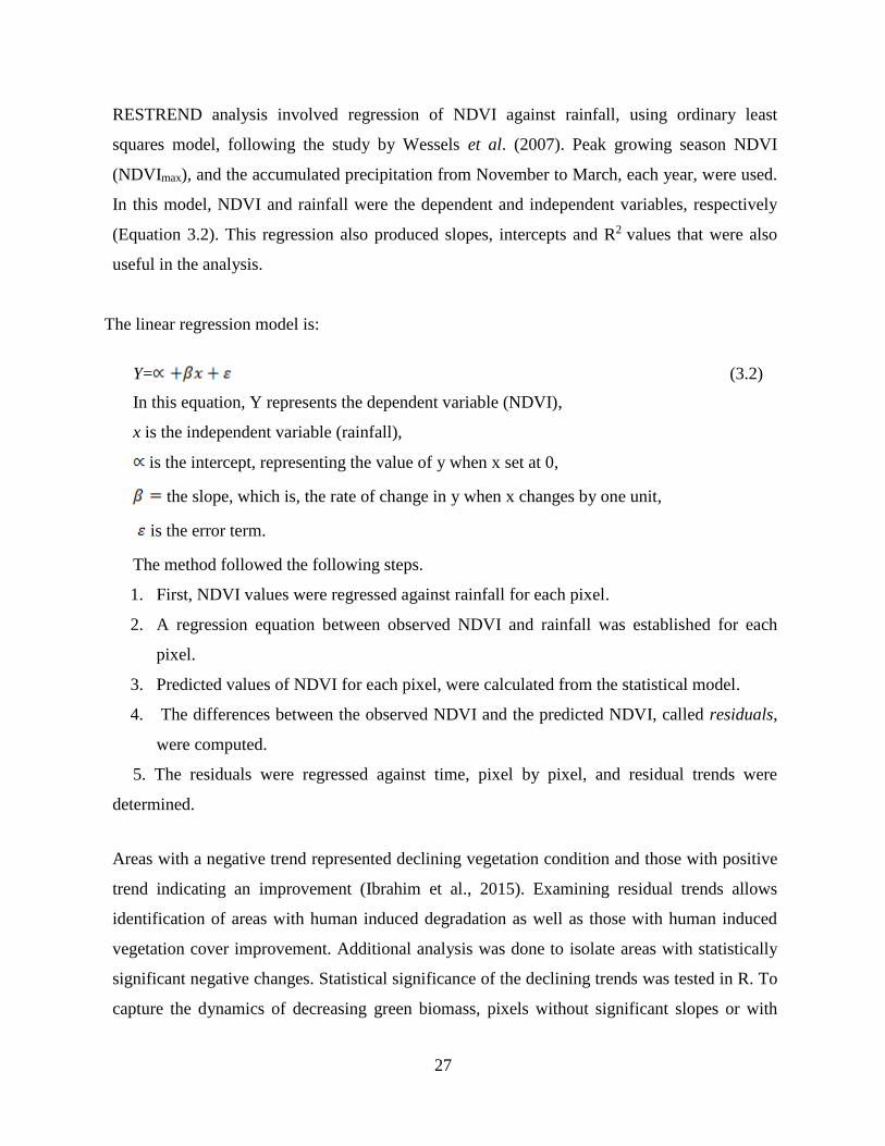
27
RESTREND analysis involved regression of NDVI against rainfall, using ordinary least
squares model, following the study by Wessels et al. (2007). Peak growing season NDVI
(NDVImax), and the accumulated precipitation from November to March, each year, were used.
In this model, NDVI and rainfall were the dependent and independent variables, respectively
(Equation 3.2). This regression also produced slopes, intercepts and R2 values that were also
useful in the analysis.
The linear regression model is:
Y= (3.2)
In this equation, Y represents the dependent variable (NDVI),
x is the independent variable (rainfall),
is the intercept, representing the value of y when x set at 0,
the slope, which is, the rate of change in y when x changes by one unit,
is the error term.
The method followed the following steps.
1. First, NDVI values were regressed against rainfall for each pixel.
2. A regression equation between observed NDVI and rainfall was established for each
pixel.
3. Predicted values of NDVI for each pixel, were calculated from the statistical model.
4. The differences between the observed NDVI and the predicted NDVI, called residuals,
were computed.
5. The residuals were regressed against time, pixel by pixel, and residual trends were
determined.
Areas with a negative trend represented declining vegetation condition and those with positive
trend indicating an improvement (Ibrahim et al., 2015). Examining residual trends allows
identification of areas with human induced degradation as well as those with human induced
vegetation cover improvement. Additional analysis was done to isolate areas with statistically
significant negative changes. Statistical significance of the declining trends was tested in R. To
capture the dynamics of decreasing green biomass, pixels without significant slopes or with

28
significant positive slopes were not included in further analysis. The areas without significant
slopes are those areas where trends in vegetation greenness are associated with trends in
rainfall dynamics.
3.3 Results
3.3.1 NDVI linear trends in the Save catchment
Spatial distribution of NDVI trends in the Save catchment for the period 2000-2015 is
represented in figure 3.2A. Substantial decrease in vegetation cover (- 0.6 to - 0.1 year-1)
characterised, mainly, the central areas. The Western part of the Save valley is the most
degraded area as indicated by the dark brown colour that represents substantial decline in
vegetation cover. Areas that include Buhera South, Bikita East, Mutare South, Chipinge and
Chiredzi North had such strong negative trends. These are areas that extend along the Save river
valley. Moderately decreasing trends have been observed in North Western Chivi, Masvingo,
Mid Zaka, parts of Buhera, Gutu and parts of Chiredzi (-0.1 to -0.01 year-1). Vegetation cover
did not decrease much in those parts of the study region, as indicated by lower rates of change.
From 2000- 2015, vegetation cover increase was characteristic of mainly the northern and
eastern parts of the Save catchment. Those districts with positive trends (-0.01 to 0.6year-1)
include; Seke, Chikomba, Hwedza, Makoni, Mutasa, part of the Eastern Highlands and Southern
Chiredzi. Some areas in Masvingo, northern Wedza, and Chirumanzu showed negative trends,
interspersed between areas with positive trends.

29
Figure 3.2 NDVI trends in the Save Catchment where A. is a rate of change in normalised
difference vegetation index (NDVI) as a function of time (year) in the Save catchment of
Zimbabwe and B. shows significant NDVI trends (p<0.05). No change areas are shown in white.
Table 3.1 shows the areal extent and percentages of NDVI trend values for each category in
figure 3.2A. Areas that show substantial decrease in vegetation constitute 15% of the area. The
area with increasing vegetation covers 35% of the study region. The remaining area (50%)
shows moderate decrease. Therefore, 65% of the region’s vegetation is degraded, from moderate
degradation (50%) to substantial degradation (15%) whilst 35% of the region’s vegetation
showed improvement during the period of study. Spatially, land area of about 6084140 ha lost
greenness over the years. This area included areas with moderate and substantial decrease.
Conversely, a land area of approximately 3,233,710 ha showed an improvement in greenness
from 2000-2015 (table 3.1). The area covered by decreasing trend, that is negative trend, is
larger than the area showing a positive trend (table 3.1).

30
Table 3. 1 Spatial distribution of normalised difference vegetation index (NDVI) change trend
___________________________________________________________________________
Area (ha) % of total area
_____________________________________________________________________
Substantial decrease 1,438,870 ` 15
Moderate decrease 4,645,270 50
Increase 3,233,710 35
Total 9,317,850 100
_____________________________________________________________________
Negative significant slopes were also depicted during the same period (figure 3.2B) in some
parts of the area, usually coinciding with the boundaries of the semi-arid regions. Significant
linear regression slope values of NDVI over 2000-2015 were mapped in figure 3.2B where
white areas represented statistically non-significant trends. Based on the 5% threshold (p< 0.05),
the area with a decline in vegetation during the 16 year-period, amounts to 6,388,50 ha (about
6.9% of the study region), whereas about 90,493.7 ha (about 1% of the study region) exhibits an
increase in vegetation productivity (table 3.2).
Table 3. 2 Percentage of pixels in the Save Catchment that exhibited positive and negative
change trends in the normalised difference vegetation index (NDVI) dataset at 95% level of
significance.
_______________________________________________________________________________
Area (ha) Significant pixels (%)
_______________________________________________________________________
Positive trends / Increasing 90,493.7 1
trend
Negative trends / Decreasing 638,850 6.9
trend
_______________________________________________________________________
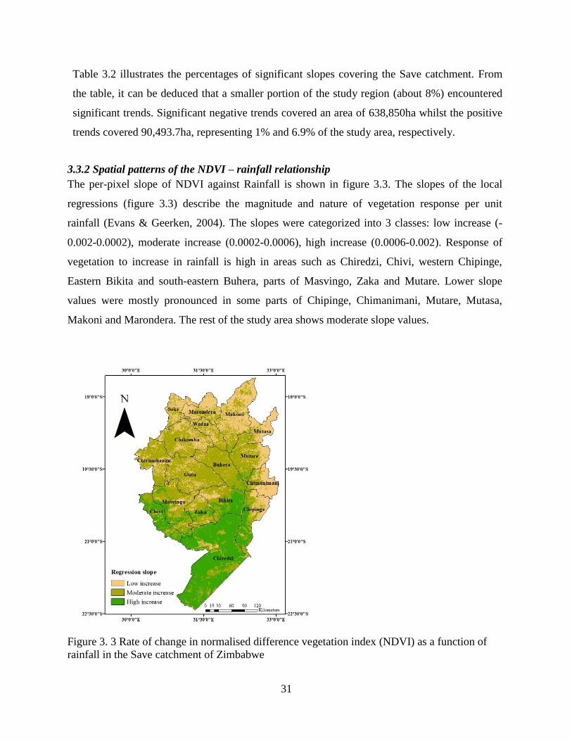
31
Table 3.2 illustrates the percentages of significant slopes covering the Save catchment. From
the table, it can be deduced that a smaller portion of the study region (about 8%) encountered
significant trends. Significant negative trends covered an area of 638,850ha whilst the positive
trends covered 90,493.7ha, representing 1% and 6.9% of the study area, respectively.
3.3.2 Spatial patterns of the NDVI – rainfall relationship
The per-pixel slope of NDVI against Rainfall is shown in figure 3.3. The slopes of the local
regressions (figure 3.3) describe the magnitude and nature of vegetation response per unit
rainfall (Evans & Geerken, 2004). The slopes were categorized into 3 classes: low increase (-
0.002-0.0002), moderate increase (0.0002-0.0006), high increase (0.0006-0.002). Response of
vegetation to increase in rainfall is high in areas such as Chiredzi, Chivi, western Chipinge,
Eastern Bikita and south-eastern Buhera, parts of Masvingo, Zaka and Mutare. Lower slope
values were mostly pronounced in some parts of Chipinge, Chimanimani, Mutare, Mutasa,
Makoni and Marondera. The rest of the study area shows moderate slope values.
Figure 3. 3 Rate of change in normalised difference vegetation index (NDVI) as a function of
rainfall in the Save catchment of Zimbabwe
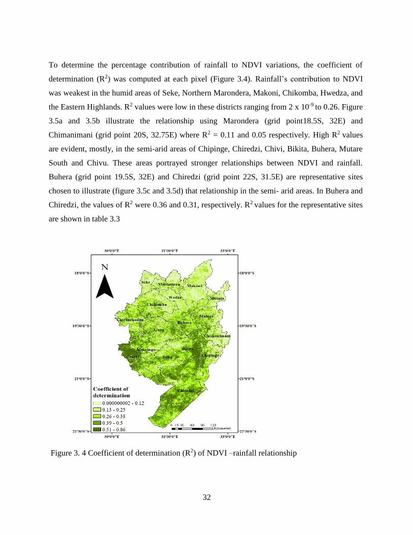
32
To determine the percentage contribution of rainfall to NDVI variations, the coefficient of
determination (R2) was computed at each pixel (Figure 3.4). Rainfall’s contribution to NDVI
was weakest in the humid areas of Seke, Northern Marondera, Makoni, Chikomba, Hwedza, and
the Eastern Highlands. R2 values were low in these districts ranging from 2 x 10⁻⁹ to 0.26. Figure
3.5a and 3.5b illustrate the relationship using Marondera (grid point18.5S, 32E) and
Chimanimani (grid point 20S, 32.75E) where R2 = 0.11 and 0.05 respectively. High R2 values
are evident, mostly, in the semi-arid areas of Chipinge, Chiredzi, Chivi, Bikita, Buhera, Mutare
South and Chivu. These areas portrayed stronger relationships between NDVI and rainfall.
Buhera (grid point 19.5S, 32E) and Chiredzi (grid point 22S, 31.5E) are representative sites
chosen to illustrate (figure 3.5c and 3.5d) that relationship in the semi- arid areas. In Buhera and
Chiredzi, the values of R2 were 0.36 and 0.31, respectively. R2 values for the representative sites
are shown in table 3.3
Figure 3. 4 Coefficient of determination (R2) of NDVI –rainfall relationship

33
Figure 3. 5 Regressions between NDVImax and rainfall for (a) Marondera (grid point18.5S, 32E),
(b) Chimanimani (grid point 20S, 32.75E), (c) Chiredzi (grid point 22S, 31.5E) and (d) Buhera
(grid point 19.5S, 32E).

34
Table 3. 3 Coefficient of determination (R2) of the relationship between rainfall and NDVI.
_____________________________________________________________________________
Station R2
__________________________________________________________________________________________________________
Buhera 0.36
Chimanimani 0.05
Chiredzi 0.31
Marondera 0.10
______________________________________________________________________
The intercept (figure 3.6) indicates the NDVI value from the regression model when the
rainfall amount is set at zero. The intercepts were computed to consider variations in
relationships between NDVI and rainfall due to other influences, which include, different soils
as well as vegetation types. The intercepts in non-degraded areas of Chipinge, Chimanimani,
Mutasa, Makoni and Marondera were higher than those in degraded low rainfall areas.
Intercept parameters increased from very arid to humid areas of Save Catchment. The slope
parameter decreased in the same direction. Most areas with the lowest slope values when
NDVI was regressed against rainfall had highest intercepts.

35
Figure 3. 6 Intercept of the relationship between NDVI and rainfall in the Save catchment of
Zimbabwe
3.3.3 Spatial patterns of the NDVI residual trends
The NDVI residual trends, defined earlier as the observed minus the predicted NDVI at each
pixel, was analysed using the ordinary least squares model. Figure 3.7 is a map of the spatial
distribution of residual trends, showing vegetation productivity trends, which are either positive
or negative, when the effect of rainfall has been removed. Higher regression slopes of residuals
existed in the Northern districts (slope>0.002) of the Save Catchment. Negative trends in NDVI
are clustered in the central and southern regions. Negative residual trends are in eastern Bikita,
south-eastern Buhera, eastern Chipinge, south of Mutare, Chimanimani and northern Chiredzi.
These areas stretch along the Save Valley.
Figure 3. 7 Slope, which is the rate of change in normalised difference vegetation index (NDVI)
residuals as function of time (2000-2015), in the Save catchment of Zimbabwe

36
Table 3. 4 Spatial distribution of normalised difference vegetation index (NDVI) residual trends
_________________________________________________________________________
Area (ha) % of total area
__________________________________________________________________
Negative (-0.03- -0.002) 1,705,910 18.3
Moderate (-0.001-0.002) 4,469,150 48
Positive (0.003-0.04) 3,129,390 33.6
____________________________________________________________________
The percentages of total area representing different classes of residual trend values were
calculated for every district (table 3.5). This was meant to determine the district that was mostly
affected by human induced degradation. From table 3.5, the districts were arranged in
descending order, from the heavily degraded to the least degraded. It can be deduced that
Chiredzi experienced the most human induced degradation over the study period. 60.5% of
Chiredzi district was covered by negative residual trends. The least degraded was Seke district
which had 6.5% of the district area experiencing human induced degradation.
Table 3. 5 Level of human induced vegetation degradation in every district within the Save
catchment of Zimbabwe
_____________________________________________________________________________________
District Total area (ha) % of total area affected by degradation
______________________________________________________________________________
Negative Moderate Positive
______________________________________________________________________________
Chiredzi 1,752,562 60.5 23.8 15.8
Bikita 517,156.5 52.7 28.8 18.5
Buhera 533,419 50.4 23 26.6
Chipinge 515,900 48.3 28.7 23
Mutare 561,831 45 32.8 22.1
Chivi 354,099.7 41.5 46.2 12.3
Chimanimani 327,875 29.6 39.8 30.6
Wedza 257,524.8 25.4 41.6 33
Makoni 782,569 19.8 42.5 37.7
Zaka 309,918.3 19.4 55.2 25.4

37
Mutasa 251,431.3 18.2 32.9 48.8
Marondera 352,131 18.2 35 46.7
Masvingo 687,012 18 41 41
Gutu 710,437 16.8 38.9 44.3
Chirumanzu 469,187.3 14.1 31.3 54.6
Chikomba 660,868.5 7.7 34.9 57.3
Seke 253,806.3 6.5 26.8 66.7
3.3.4 Comparison of RESTREND with raw vegetation index trends
RESTREND and raw NDVI trend analysis both show considerable areas covered by greening
trends (38% and 35% respectively) (table 3.6). Negative raw NDVI trends, however, covered a
greater percentage of the study area (65%) than the negative residual trends (26%) although
there is similarity in their spatial distribution patterns.
Table 3. 6 The percentage of pixels that increased or decreased, in the NDVI linear trend analysis
and the RESTREND analysis methods
__________________________________________________________
% increasing % decreasing
_____________________________________________________
NDVI trend 35 65
Residual trend 38 26
_____________________________________________________
3.3.5 Severity of vegetation degradation
Pixels recording significant negative residual trends (p< 0.05) were mapped in figure 3.8 and
used to formulate different degradation classes following Vlek et al. (2008). Pixels that had a
statistically significant, decreasing trend constituted 38.8% of the study area, covering 3,609,955
ha. Approximately 3.6% of the study area was severely degraded, 12.8% was moderately
degraded and 22.4% was lightly degraded. The corresponding areas of significant degradation
were 332,575 ha, 1,189,820 ha, and 2,087,560, respectively. Table 3.7 illustrates the
geographical extent of the catchment affected by significant human-induced degradation
processes.

38
Figure 3. 8 Areas showing significant negative residual trends at 95% significance level
* Areas with non-significant changes are shown in white colour.
Table 3. 7 Degradation severity in Save catchment (percentage of area by severity class)
__________________________________________________________________________
Degree of Degradation Area (ha) Percentage (%)
_________________________________________________________________________
Severe 332,575 3.6
Moderate 1,189,820 12.8
Light 2,087,560 22.4
Total 3,609,955 38.8

39
3.4 Discussion
From the analysis of NDVImax trends, vegetation cover decline was observed in most parts of the
Save Catchment, during the period 2000-2015 (figure 3.2A). Since significant negative trends
were also exhibited during the same period (figure 3.2B) and considering high precipitation
variability in the dry areas (Mambo & Archer, 2007), it suggests that this decrease could partly
be as a result of rainfall anomalies. Buhera, Bikita, Masvingo, Chiredzi, Zaka and Chivi, and
some parts of Chipinge and Chimanimani experienced wide coverage of negative NDVI trends.
These are the dry regions in Zimbabwe (Vincent & Thomas, 1960). They lie in natural regions 3,
4 and 5, characterised by unreliable, low and erratic rainfall that averages between 400mm and
600mm per annum (Climate handbook of Zimbabwe, 1981). The existence of patches of
degraded land interspersed between positive trends in humid areas of Chimanimani and Chipinge
(fig 3.2A) can be explained in terms of vulnerability of some arid areas in the districts, given that
Chipinge and Chimanimani have all the five agro-ecological regions (FAO, 2012). Zimbabwe
has experienced increased frequency of drought associated with Elnino events in recent decades
with, on average, 1-3 droughts experienced every 10 years. Droughts have occurred in 2001/2,
2002/3, 2004/5, 2006/7 seasons (Simba et al., 2012; Richardson, 2007). These drought years
could have contributed to overall negative NDVI trends which are widespread in most parts of
the Save Catchment because an arid climate hinders vegetation growth (Li et al., 2015). Tropical
cyclones, a weather scenario associated with both Elnino and La Nina years also help explain
strong negative trends in these semi-arid regions where associated floods caused massive
vegetation destruction, mainly, in the districts of Mutare, Chimanimani, Chipinge, Chiredzi, and
Zaka (FAO, 2012). Cyclone Eline, associated with extensive and disastrous floods was
experienced in the year 1999/2000 and above normal mean rainfall (942mm) was recorded in
those districts in that growing season (FAO, 2012). Vegetation, that included vast areas of
plantations was destroyed in districts of Chimanimani and Chipinge where an estimate of 3,340
hectares of timber was damaged, which, according to the Timber Producers Association, was an
equivalent of a year’s harvest (Reason & Keible, 2004). Coupled with the negative impacts of
drought, these destructive floods contributed immensely to the widespread negative trends in the
Save Catchment. Poor soils could also have accelerated the degradation in these semi-arid
regions. Most communal lands that have suffered huge biomass losses have granite derived
sandy soils that are highly erodible (FAO, 2012). The communal areas of Chiredzi, characterised

40
by sandy soils (Cunliffe et al., 2012) have evidence of widespread degradation, presumably,
because of these poor soils.
With all the above factors pointing towards increased vegetation degradation in these areas,
Chimanimani district clearly shows some positive trends in vegetation recovery. Tropical
rainforests are still evident in the moist foothills of Chimanimani, with woodlands dominating
the more exposed or drier sites (Timberlake et al., 2016). An example is the Maronga Forest
Reserve. Despite the fire of 1992, the 1991/1992 drought and the effects of Cyclone Eline in
2000, which caused widespread forest destruction, the regeneration capacity of the landscape is
promoting new forest growth (Timberlake et al., 2016). The Northern districts of the Save
catchment, most of which lie in regions 2 and 3, as well as region 1 areas of the Eastern
highlands, also experienced positive NDVI trends during the study period. These high rainfall
areas, complemented by deep fertile soils, are characterised by high photosynthetic activity
which explains vegetation improvements over the years. The distribution patterns of the raw
NDVI trends follow rainfall patterns, revealing the effect of climate on terrestrial ecosystems
dynamics.
According to Li et al. (2004), NDVI and rainfall relationships can explain ecosystem
productivity variations and deterioration in land condition in dry areas. The distribution of
regression slopes of NDVI against rainfall, in this study, agreed with those reported in other
studies (Ibrahim, 2017; Wessels, 2007; Evans & Geerken, 2004; Lambin, 2001). The dry areas of
the Save Catchment exhibited strong linear relationships as shown by high slope values in those
semi-arid regions. The slopes indicate the amount of change in vegetation cover per unit change
in rainfall (Ibrahim, 2017). Pixels in the semi-arid regions of Buhera, Bikita, Chipinge and
Chiredzi have higher regression slope values compared to the high rainfall mountainous areas
which are covered by the evergreen miombo forests. These findings indicate that vegetation in
dry areas is highly responsive to the high rainfall variability (Lu et al., 2015; Wessels et al.,
2007). High rainfall zones that include humid forest areas of Chimanimani and Chipinge
exhibited weak responses. This is largely because annual rainfall amounts usually exceed a
certain threshold, above which vegetation becomes non-responsive (Lu et al., 2015). Such high-
altitude areas, characterised by deep loamy soils that have high water holding capacity and are

41
not easily eroded, have sustained vegetation growth even in low rainfall regimes (FAO, 2012).
Given the varied landscapes of the two districts, areas in the valleys, that are mainly in region 4
and 5 are characterised by sand to sandy loam soils that are strongly leached, have low water
holding capacities and that do not sustain growth (FAO, 2012). That explains lower slope values
in those semi-arid areas of the two districts. Similarities were identified in the distribution
patterns of NDVI-rainfall slopes and R2 values. Those areas receiving large amounts of rainfall
and characterised by low R2 values coincided with low responsiveness to increase in rainfall.
Wetter regions exhibit low NDVI-rainfall correlation, since saturation point is attained, beyond
which further greening would not occur, despite an increase in water supply (Chikore & Jury,
2010). Because Manicaland is home to indigenous forests, as well as commercial plantations of
exotic trees and tea estates, proper management can help explain the low R2 values. Most humid
areas also had the highest intercepts, whilst very low rainfall areas had low intercepts, suggesting
the importance of rainfall as determinant of vegetation growth in semi-arid regions (Evans &
Geerken, 2004). These results reveal rainfall as highly influential in vegetation production in the
Save catchment, a factor that may mask negative impacts of human-induced degradation
processes (Wessels, 2007).
According to Wessels et al. (2007), assessing vegetation changes without removing rainfall
impact has misleading implications for landscape management. This is because human beings
alter the structure of landscapes, mainly through various land use practices. During the study
period, considerable areas (18.3%) exhibited negative residual trends. These were mainly
concentrated in Buhera, Mutare, Bikita, Chipinge, parts of Chimanimani and Chiredzi and the
areas that also experienced significant degradation. Chiredzi was the most degraded district,
where negative trends covered 60.5% of the district area, with the least degraded being Seke
district (6.5%) (Table 3.5). Severe degradation is evident mostly in the Save Valley, with Bikita,
Chipinge, Chiredzi and part of Buhera districts being the mostly affected. In agreement with
these findings, Mambo & Archer (2007) also observed degradation in Buhera district with high
susceptibility to the south-eastern part of the district. This study also revealed portions of severe
degradation in Buhera, coinciding with almost the same areas of high susceptibility found by
Mambo & Archer (2007). They also revealed a large portion of Buhera district under cultivation
from 1992 data, with woodlands continuously being cleared for agricultural expansion. Prince et

42
al. (2009) also identified degradation, reflected by local net scaling (LNS) maps, in most
communal areas of the Save. Clearance of forests for the establishment or expansion of
agricultural land, together with intensive fuelwood extraction is rapidly depleting communal
areas of vegetation resulting in soil erosion. This breakdown in community resource
management also results in siltation of water reservoirs such as the Save river, affecting the
river’s capacity as well as the aquatic ecosystems (Makwara & Gamira, 2012).
Degradation patterns on the RESTREND map (fig 3.7) agree with results by Prince et al.
(2009). From their studies, commercial farms stretching through Chivu, north of Harare,
Marondera and even those in Chiredzi exhibit good vegetation cover. Some degradation was
detected in these commercial lands. In most of those commercial areas where rainfall is high,
low NPP was related to improper agricultural practices among the neighbouring subsistence
farmers (Prince et al., 2009). This also helps explain patches of degraded areas, mainly in some
areas of Marondera, Wedza, Chimanimani and Chipinge that have vast stretches of commercial
farms and plantations. Particular examples were to the southern part of Chiredzi where there is
a clear distinction between greening areas of Triangle and Chisumbanje sugarcane estates and
browning, communal areas of Chiredzi district. Zimbabwe has had a long history of neglected,
poor degraded communal areas (Scoones, 2002).
According to Mambo & Archer (2007), investigating susceptibility t o degradation requires
investigation of other factors, especially the human factors (Eswaran et al., 1997). Mutasa
district, has the highest population density of 66 persons per km2. This area should be one of the
most severely degraded regions. On the contrary, the district is lightly degraded and there are
just patches of degraded land. There are more positive residual trends (48.8%) than negative
residual trends (18.2%) covering Mutasa district. This supports the view that high concentration
of population may not always lead to the deterioration of land condition (Eswaran et al., 2001).
This is also in agreement with Bai et al. (2008), whose research results, on a global scale, show
an improvement in vegetation condition in densely populated areas of SSA. Voortman et al.
(2000) argued that, high population density in SSA characterises the most fertile areas,
particularly, mountain slopes. These fertile areas would support vegetation growth. Therefore,
degradation is determined by what the occupants do to the land and not just population pressure

43
(Eswaran et al., 2001).
In this study, there were areas that experienced negative correlation between population density
and vegetation condition, notably, in communal areas of Chipinge district (50 persons km-2) and
Buhera district (46 persons km-2) (https://www.citypopulation.de/php/zimbabwe-admin.php)
whose negative residual trends occupied 48.3% and 50.4% of the study area (table 3.5),
respectively. Excessive pressure in the overcrowded communal lands of these areas is the leading
factor in the degradation process. There are also areas with low population densities that have
been affected by human induced degradation. These include parts of Chiredzi district (16 persons
per km2) and Bikita district (31persons per km2). In these areas human induced degradation was
experienced in 60.5% and 52.7% of the study area (table 3.5), respectively. This agrees with
Mambo & Archer (2007) who detected high indication of degradation in wards of Buhera
district having the lowest population density. Most of these areas are unsuitable for agriculture
because of topographical and soil constraints. Unfavorable topography and soil conditions pose
inherent restrictions on exploitation and habitation (Vlek et al., 2008; Wang, 2016).
The interaction that takes place between humans and their environment, inevitably results in
degradation, mainly because of wind and water soil erosion, chemical reactions and soil
disturbance by animals. Negative land use practices (Lal, 2001) include cultivation of marginal
lands like semi-arid areas, steep slopes and shallow soils. The utilisation of marginal lands is a
result of an increasing number of farming communities in need of agricultural land, yet there is a
decline in availability of arable land (Lal, 2000). Other factors include traditional grazing
systems, deforestation and firewood collection. Further influences arise from political, socio-
economic and historical backgrounds. Therefore, poor resource utilisation works hand in hand
with biophysical influences like soil properties, climatic characteristics, topography and
vegetation types, making the task of isolating the role of physical from anthropogenic factors
more difficult (Einsele and Hinderer, 1998) .

44
3.5 Conclusions
Based on the findings of this study, residual trend analysis method was demonstrated to be useful
in distinguishing between climatic and human induced factors as drivers of vegetation
degradation in semi-arid landscapes. In this regard, this study has revealed that:
• Climate is an important factor in vegetation cover changes, particularly, in semi-arid
areas. Vegetation in dry areas is responsive to rainfall variations. The responsiveness is
not the same in humid areas where a weak relationship between vegetation and rainfall is
observed.
• Vegetation significantly degraded in 38.8% of the Save catchment as a result of human
activities.
• The degrading trend in vegetation was most severe in the central districts of the Save
catchment.
• Vegetation cover decline can successfully be used as a proxy of vegetation degradation.
However, it is not comprehensive in characterising vegetation degradation. As a
recommendation, further studies should examine vegetation degradation using other
proxies, for example, reduced soil organic carbon, wetland decline, and others.
• As a recommendation, further studies should investigate the influence of soil
characteristics and topographic factors on vegetation cover in the fragile ecosystems of
the Save catchment in the context of vegetation degradation.

45
CHAPTER FOUR: Objectives reviewed and conclusions
4.1 Introduction
This research aimed at determining the degree to which human activities influence the decline in
land condition in the Save Catchment, Zimbabwe, using NDVI time-series data. This chapter
evaluates the objectives presented in Chapter one against findings. Furthermore, the chapter
highlights major conclusions, limitations and recommendations for future research.
4.2 Objectives reviewed
Overview of the application of satellite earth observations in assessing and monitoring
vegetation degradation.
The research reviewed vegetation degradation monitoring across landscapes. The extent and rate
of degradation was reviewed from planetary to local scales. Identification of the exact causes of
decline in land productivity was described as challenging because of interactions between many
triggering factors. However, interactions of climatic changes, unsustainable land management
and land tenure systems have been regarded as major contributors to the deteriorating quality of
land. Negative impacts of this degradation result in millions of dollars being lost annually. Large
populations suffer from poverty and food insecurity. Literature has also revealed that, although
global assessment of vegetation degradation started a long time ago (1980s), estimates of its
extent and severity have not been consistent. The varied definitions regarding the process and
lack of standardized method for its assessment has led to inconsistencies in interpretation of
results. Early assessments have largely been questioned since the results tended to be local and
relied on opinions from experts. The results lacked reliable supporting data especially in the
early stages of the process. Traditional assessment methods, for example, field surveys were
criticized for being costly and for failure to provide a global view of ecosystem changes.
Mankind has excelled in determining vegetation degradation at various spatial scales, following
the development of satellite earth observation technologies and computing systems. Remote
sensing technologies, especially the use of NDVI time-series, have been advocated as the most
viable way in vegetation degradation mapping. This was revealed to be because of its ability to
provide up to date assessments at scales relevant for decision making. Although NDVI, a widely
used proxy of vegetation degradation, was extensively applied in vegetation degradation
monitoring, its use in semi-arid regions was mainly limited by rainfall variability. The
46
application of Residual trend method in disentangling the impact of rainfall was reviewed. The
method was effective in separating vegetation degradation due to human activities.
The effectiveness of RESTREND method in detecting human induced vegetation
degradation.
Using ordinary least squares regression model, vegetation degradation trends were established
from NDVI-time relationships. Areas experiencing vegetation improvement or loss due to both
natural and anthropogenic causes were determined from this analysis. From this study, 65% of
the catchment was covered by negative trends whereas 15% experienced improvement. The map
of significant NDVI trends demonstrated, in part, the influence of human actions in vegetation
cover growth. Regression model analysis of NDVI and rainfall showed that vegetation growth
was strongly influenced by climatic variations in semi-arid areas of the Save catchment where
regression slope values and R2 values tended to be higher than in humid areas. Higher intercepts
were characteristic of northern districts and mountainous areas of the eastern districts and drier
areas that were largely dependent on rainfall for growth, had low intercept values. The regression
slope, intercept maps and R2 portrayed the important role played by rainfall variations in
determining ecosystem productivity. Residual trend analysis method was effective in separating
the influence of rainfall and human activities on degradation trends. A clear distinction between
degraded areas, improved areas and areas with moderate changes was mapped using this
technique. From the analysis of residual trends, 18.3% and 33.6% of the study area encountered
degradation and improvement, respectively. The larger portion of negative raw NDVI trends
compared to negative residual trends reflects the important role climate plays in influencing
vegetation growth in very low rainfall parts of the Save catchment, sometimes masking the
human influences. Statistical analysis established significantly degraded pixels, from which
severity classes were produced and mapped. Severe degradation was observed to the east of
Bikita, west of Chipinge and Northern Chiredzi. The drivers of the changes were suggested using
information on agro-ecological zones, soil types, vegetation cover as well as population density
statistics. RESTREND method effectively separated areas of degradation due to human
activities.

47
4.3 Conclusions
The development of satellite earth observation technologies, together with computing systems,
has enabled the determination of vegetation degradation at various spatial scales, because of its
ability to provide up to date assessments at scales relevant for decision making. This study
examined long-term MODIS NDVI data to assess changes in vegetation in Save catchment from
2000 to 2015. Time-series analysis of NDVI trends revealed large areas experiencing vegetation
cover loss. Vegetation growth was strongly influenced by climatic variations. Existence of
significant trends indicated the role humans play in promoting land productivity losses.
RESTREND method was effective in isolating climatic influences, allowing for the mapping of
alteration of the ecosystems which was a result of human activities. As a recommendation, future
studies on long term vegetation changes should employ methods that consider breaks in the trend
patterns, because this aspect is not handled well using the RESTREND method.
The use of MODIS data, that is available for all the years, allowing time-series analysis, is not
without limitations. Its spatial resolution is relatively coarse and lacks detail required for the
quantification of small-scale vegetation cover changes. Future studies should utilise higher
resolution data to enhance quality of analysis results. Because some areas have been identified as
severely degraded in the Save catchment, policy action is needed to rehabilitate those areas and
to combat the process. Land management policies should be effectively implemented, especially
in communal agricultural lands, where land tenure system does not encourage investment in the
land.
48
References
Adimassu, Z., Mekonnen, K., Yirga, C. & Kessler, A. 2014. The effect of soil bunds on runoff,
losses of soil and nutrients, and crop yield in the central highlands of Ethiopia. Land
Degradation & Development, 25, 554–564.
Albalawi, E. K. & Kumar, L. 2013. Using remote sensing technology to detect, model and map
desertification: A review. Journal of Food, Agriculture and Environment, 11, 791-797.
Bai, Z. B., Dent, D. L., Olsson L. & Schaepman, M. E. 2008. Proxy global assessment of land
degradation. Soil use and management, 24: 223-234.
Bai, Z. G. & Dent, D. L. 2007. Land degradation and improvement in South Africa. Report 2007
⁄ 03, ISRIC – World Soil Information, Wageningen.
Berry, L., Olson, J. & Campbell, D. 2003. Assessing the extent, cost and impact of land
degradation at the national level: findings and lessons learned from seven pilot case
studies. https://www research gate. Net/publication/272682048.
Burrell, A. L., Evans, J. P. & Liu, Y. 2017. Detecting dryland degradation using Time-series
Segmentation and Residual Trend analysis (TSS-RESTREND). Remote Sensing of
Environment, 197, 43–57.
Camberlin, P. Martin, N., Philippon, N. & Richard, Y. 2008. Determinants of the interannual
relationships between remote sensed photosynthetic activity and rainfall in tropical
Africa. Remote Sensing of Environment, 106, 199–216.
Chikore, H. & Jury, M.R. 2010. Intraseasonal Variability of Satellite-based Rainfall and
Vegetation over Southern Africa University of Zululand, KwaDlangezwa, South Africa.
Climate handbook of Zimbabwe, 1981. Meteorological services department, Harare.
Cunliffe, R., Muller, O. & Mapaura, A. 2012. Vegetation survey of Gonarezhou National Park.
Zimbabwe Final Report.
D’Odorico, P., Okin, G.S. & Bestelmeyer, B.T. 2012. A synthetic review of feedbacks and
drivers of shrub encroachment in arid grasslands. Ecohydrology 5 (5), 520e530.
http://dx.doi.org/ 10.1002/eco.259.
Dalu, T., Tambara, E. M., Chari, L. & Nhiwatiwa, T. 2013. Modeling sedimentation rates of
Malilangwe Reservoir in the south-eastern lowveld of Zimbabwe. Appl Water Sci, 3,133–
144.
De Jong, S. and Epema, G. F. 2011. Imaging Spectrometry for Surveying and Modelling Land
Degradation. In: van der Meer, F. D. & De Jong, S. M. (eds): Imaging Spectrometry.
Dord-recht: Springer.
Dube, T., Mutanga, O., Sibanda M., Seutloali, K. & Shoko C. 2017. Use of Landsat series data to
analyse the spatial and temporal variations of land degradation in a dispersive soil
environment: A case of King Sabata Dalindyebo local municipality in the Eastern Cape
Province, South Africa.
Dubovyk, O. 2017. The role of Remote Sensing in Land Degradation Assessments:
Opportunities and Challenges. European Journal of Remote Sensing, 50, Issue 1.
Eckert, S., Hüsler, F., Liniger, H. & Hodel, E. 2015. Trend analysis of MODIS NDVI time-
series for detecting land degradation and regeneration in Mongolia. Journal of Arid
Environments, 113, 16-28.

49
Einsele, G. & Hinderer, M. 1998. Quantifying denudation and sediment accumulation systems
(open and closed lakes): Basic concepts and first results. Paleogeography,
Paleoclimatology, Paleoecology 140, 7–21.
Ensor, L. A. & Robeson, S. M. 2008. Statistical Characteristics of Daily Precipitation:
Comparisons of Gridded and Point Datasets. Journal of Applied Meteorology and
Climatology, 47, Indiana University
Eswaran, H., Lal, R. & Reich, P. F. 2001. Land degradation: an overview. In Responses to land
Degradation. Proceedings of 2nd International Conference on Land Degradation and
desertification, Khon Kaen, Thailand. Oxford Press, New Delhi, India.
Evans, J. & Geerken, R. 2004. Discrimination between climate and human-induced dryland
degradation. Journal of Arid Environments, 57(4), 535-554.
FAO.1978. Report on the Agro Ecological Zones Project. Volume.1. Methodologies and Results
for Africa. Rome. FAO Publication, World Soil Resources Report. 158pp.
FAO, 2012. Assessment of the Impact of Cyclone Eline (February 2000) on the Food,
Agriculture and Natural Resource Sector in Zimbabwe.
FAO, 2015. Status of the World’s soil Resources. 2015 International year of soils.
Farrar, T.J., Nicholson, S.E. & Lare, A.R. 1994. The influence of soil type on the relationships
between NDVI, rainfall, and soil moisture in semiarid Botswana. II. NDVI response to
soil moisture. Remote Sens. Environ., 50, 121–133.
Fensholt, R. & Sandholt, I. 2005. Evaluation of MODIS and NOAA AVHRR vegetation indices
with in situ measurements in a semi-arid environment. International Journal of Remote
Sensing, 26(12), 2561–2594.
Forkel, M., Carvalhais, N., Verbesselt, J., Mahecha, M.D., Neigh, C.S.R. & Reichstein, M. 2013.
Trend Change Detection in NDVI Time-series: Effects of Inter-Annual Variability and
Methodology Remote Sensing, 5, 2113-2144; doi:10.3390/rs5052113.
Gao, J. & Liu, Y. 2010. Determination of land degradation causes in Tongyu County, Northeast
China via land cover change detection. International Journal of Applied Earth
Observations and Geoinformation, 12(1), 9–16.
GEF. 2006. Global Environmental Facility: protecting the global environment—Africa, http://
German Technical and Development Cooperation GTZ 2005. Fact sheets desertification: Africa
convention project to combat desertification.
Global Mechanism of the UNCCD, 2018. Country Profile of Zimbabwe. Investing in Land
Degradation neutrality. Making the Case. An overview of Indicators and Assessments.
Bonn. Germany.
Gore, C., Katerere, Y., Moyo, S., Mhone, G., Mazambani, D. & Ngobese, P. 1992. The case for
sustainable development in Zimbabwe: Conceptual problems, conflicts, and
contradictions, report prepared for the United Nations Conference on Environment and
Development (UNCED), 159pp. Harare: Environmental and Development Activities
(ENDA–Zimbabwe) and Regional Network of Environmental Experts (ZERO).
Greenland, D. J., Bowen, G., Eswaran, H., Rhodes, R. & Valentin, C. 1994. Soil, water, and
nutrient management research: a new agenda. IBSRAM Position Paper. IBSRAM,
Bangkok, Thailand.
Harris, I., Osborn, T. J., Jones, P. D. & Lister, D. 2014. Updated high-resolution grids of
monthly climatic observations—The CRU TS3.10 Dataset. Wiley Online Library. DOI:
10.1002/joc.3711.
50
Hassan, M. S., UL-Islam, S. M. & Rahman, M. T. 2015. Integration of Remote Sensing and GIS
to Assess Vulnerability of Environmental Degradation in North-Western Bangladesh.
Journal of Geographic Information System, 2015, 7, 494‐505.
Herrmann, S. M., Anyamba, A. & Tucker, C. J. 2005. Recent trends in vegetation dynamics in
the African Sahel and their relationship to climate. Global Environmental Change, 15,
394-404.
Higginbottom, T. P. & Symeonakis, E. 2014. Assessing land degradation and desertification
using vegetation index data: Current frameworks and future directions. [Review]. Remote
Sensing, 6(10), 9552–9575.
Hill, J., Stellmes, M., Udelhoven, T., Röder, A. & Sommer, S. 2008. Mediterranean
desertification and land degradation. Mapping related land use change syndromes based
on satellite observations. Global and Planetary Change, 64146–157.
Hoekstra, J. M., Timothy M. Boucher, T. M., Ricketts T. H. & Roberts, C. 2005. Confronting a
biome crisis: global disparities of habitat loss and protection. Ecology Letters, 8(1), 23-
29.
Hoscilo, A., Balzter, H., Bartholomé, E., Boschetti, M., Brivio, P.A., Brink, A., Clerici, M. &
Pekel, J. F. 2014. A conceptual model for assessing rainfall and vegetation trends in sub-
Saharan Africa from satellite earth observations. Int. J. Climatol.
Huete, A. K. Didan, T., Miura, E.P., Rodriguez, X. & Ferreira, L.G. 2002. Overview of the
radiometric and biophysical performance of the MODIS vegetation indices. Remote
Sensing of Environment, 83, 195–213.
Huxman, T. E., Smith, M. D., Fay, P. A., Knapp, A. K., Shaw, M. R. & Loik, M. E. 2004.
Convergence across biomes to a common rain-use efficiency. Nature, 429, 651–654.
Ibrahim, Y., Balzter, H., Kaduk, J. & Tucker, C. 2015. Land degradation assessment using
residual trend analysis of GIMMS NDVI3g, soil moisture and rainfall in sub-Saharan
west Africa from 1982 to 2012. Remote Sensing, 7(5), 5471–5494.
doi:10.3390/rs70505471.
IFAD. 2009. The Strategic Investment Program for Sustainable Land Management in Sub-
Saharan Africa. IFAD.
Jensen, J. 2007. Remote Sensing of the Environment. Pearson Prentice Hall.
Johnson, P. M., Mayrand, K., & Paquin, M. 2006. The United Nations Convention to combat
desertification in global sustainable development governance. Governing Global
Desertification: Linking Environmental Degradation, Poverty and Participation,
Aldershot: Ashgate, 1-10.
Kapalanga, T. S. 2008. A review of land degradation assessment methods. Land restoration
programme.
Kareiva, P., Watts, S., McDonald, R. & Boucher, T., 2007. Domesticated nature: shaping
landscapes and ecosystems for human welfare. Science, 316, 1866–1869.
Khishigbayar, J., Fernández-Giménez, M.E., Angerer, J.P., Reid, R.S., Chantsallkham, J.,
Baasandorj, Y. & Zumberelmaa, D., 2015. Mongolian rangelands at a tipping point?
Biomass and cover are stable but composition shifts and richness declines after 20 years
of grazing and increasing temperatures. J. Arid Environ. 115, 100–112.
Kremer, R. G. & S. W. Running. 1993. ‘‘Community Type Differentiation Using
NOAA/AVHRR Data within a Sagebrush-Steppe Ecosystem.’’ Remote Sensing of
Environment, 46, 311–18.
51
Lal, R. 2000. Soil management in the developing countries. Soil Science, 165, 57–72.
Lal, R. 2001. Soil degradation by erosion. Land Degradation and Development 12, 519–539.
Lal, R. & Singh, B. R. 1998. “Effects of soil degradation on crop productivity in East Africa”.
Journal of Sustainable Agriculture, 13, 1, 15-36.
Lambin, E. F. & Ehrlich, D. (1997). Land-cover changes in sub-Saharan Africa (1982–1991):
Application of a change index based on remotely sensed surface temperature and
vegetation indices at a continental scale. Remote Sensing of Environment, 61, 181−200.
Le, Q. B., Nkonya, E. & Mirzabaev, A. 2016. Biomass productivity-based mapping of global
land degradation hotspots. In Nkonya, E., Mirzabaev, A. & Von Braun (Eds.), Economics
of land degradation and improvement – A global assessment for sustainable
development (55–84). Cham: Springer International Publishing.
Li, A., Wu, J. & Huang, J. 2012. Distinguishing between human-induced and
climate-driven vegetation changes: a critical application o f RESTREND
in inner Mongolia. Landscape ecol, 27, 969-982.
Li, D., Shan, J. & Li, J.G. (Eds.). 2009. Geospatial technology for earth observation. New York,
NY: Springer.
Liang, S. 2005. Quantitative remote sensing of land surfaces. John Wiley & Sons.
Liniger, H. P., Studer, R. M., Hauert, C. & Gurtner, M. 2011. Sustainable Land Management in
Practice– Guidelines and Best Practices for Sub-Saharan Africa. TerrAfrica, World
Overview of Conservation Approaches and Technologies (WOCAT) and Food and
Agriculture Organization of the United Nations (FAO).
Lotz-sisitka, H. 2010. Knowledge Questions associated with the Public Health and Climate
Change relations: Some Implications for Universities in Southern Africa. SARUA
Leadership Dialogue Series 2: 101-114.
Lu, L., Kuenzer, C., Wang, C., Guo, H. & Li, Q. 2015. Evaluation of Three MODIS-Derived
Vegetation Index Time-series for Dryland Vegetation Dynamics Monitoring. Remote
Sensing. 7, 7597-7614; doi:10.3390/rs70607597.
Makwara, E. C. & Gamira, D. (2012). About to Lose all the Soil in Zaka’s Ward 5, Zimbabwe:
Rewards of Unsustainable Land Use. European Journal of Sustainable Development, 1,
3, 457-476.
Mambo, J. & Archer, E. 2007. An Assessment of land degradation in the Save Catchment of
Zimbabwe. Royal Geographical Society, 39, 3, 380-391.
Millennium Ecosystem Assessment 2005. Ecosystem and Human wellbeing: Desertification
synthesis. In: Assessment, M. E. (ed.).
Mulinge, W., Gicheru, P., Murithi, F. & Kihlu, E. (2016) Economics of Land Degradation and
Improvement in Kenya. https://www.researchgate.net/publication/286744415.
Nachtergaele, F., Biancalani, R. & Petri, M. 2010, Land degradation SOLAW Background
Thematic Report 3.
Nagendra, H. 2001. Using remote sensing to assess biodiversity. Int. J. Remote Sens, 22, 2377–
2400.
Ndayisaba, F., Guo, H., Isabwe, A., Bao, A., Nahayo, L., Khan, G., Kayiranga, A., Karamage, F.
& Muhire, E. 2016. Inter-Annual Vegetation Changes in Response to Climate Variability
in Rwanda. Journal of Environmental Protection, 8, 464-481.
doi: 10.4236/jep.2017.84033.

52
Nemani, R. R., Keeling, C. D., Hashimoto, H., Jolly, W. M., Piper, S. C., Tucker, C. J., Myneni,
R. B. & Running, S.W. 2003. Climate-driven increases in global terrestrial net primary
production from 1982 to 1999. Science, 300, pp. 1560–1563.
Nkonya, E., Mirzabaev, A. & Von Braun, J. 2016. Economics of land degradation and
improvement – A global assessment for sustainable development. Heidelberg: Springer.
Nyamapfene, K.W. 1991. Soils of Zimbabwe. Nehanda Publishers, Harare, Zimbabwe.
Okin, G.S., Murray, B., & Schlesinger, W. H. 2001. Degradation of sandy arid shrubland
environments: observations, process modelling and management implications. Journal of
Arid Environments, 47, pp. 123–144.
Oldeman, L. R., Hakkeling, R. T. A. & Sombroek, W. G. 1990. World map of the status of
human-induced soil degradation: an explanatory note (Wageningen: ISRIC – World Soil
Information and FAO).
Pickup, G. 1996. Estimating the effects of land degradation and rainfall variation on productivity
in rangelands:an approach using remote sensing and models of grazing and herbage
dynamics. Journal of Applied Ecology, 33, 819–832.
Plisnier, P. D., Serneels, S. & Lambin, E. F. 2000. Impact of ENSO on East African Ecosystems:
A Multivariate Analysis Based on Climate and Remote Sensing Data. Global Ecology &
Biogeography, 9, 481-497.
Prince, S. D. 2002. Spatial and temporal scales for identification of desertification in
Reynolds, J. F. & Stafford Smith, D. M. eds Global desertification: do humans cause
deserts? Dahlem Workshop Report 88, Dahlem University Press, Berlin 24 – 37
Prince, S., Becker-Reshef, I. & Rishmawi, K. 2009. Detection and mapping of long-term land
degradation using local net production scaling: Application to Zimbabwe. Remote
Sensing of Environment, 113, 1046-1057.
Prince, S. D. 2004. Mapping desertification in southern Africa. In Gutman, G., Janetos, A.,
Justice, C. O., Moran, E. F., Mustard, J. F., Rindfuss, R. R., et al (Eds.), Land change
science: Observing, monitoring, and understanding trajectories of change on the Earth's
surface (pp. 163−184). Dordrecht, NL: Kluwer.
Propastin, P. A., Kappas, M., Nadiya, R. & Muratova, N. R. 2008. Evaluating trends in Spatial
relationship between NOAA/AVHRR NDVI and rainfall as computed by geographically
weighted regression: A case study from a dry region in the Middle Kazakhstan.
Purkis, S. J. & Klemas, V. V. 2011. Remote sensing and global environmental change. John
Wiley & Sons.
Qureshi, E. M., Hanjra, M. A. & Ward, J. 2013. Impact of water scarcity in Australia on global
food security in an era of climate change. Food Policy, 38136–145. http://dx.doi.org/
10.1016/j.foodpol.2012.11.003.
R Development Core Team, 2008. R: A Language and Environment for Statistical Computing. R
Foundation for Statistical Computing, Vienna, Austria. http://www.R-project.org.
Reason, C. J. C. & Keible, A. 2004. Tropical cyclone Eline and its unusual penetration and
impacts over Southern African mainland. Weather and Forecasting, 19, 789-805.
Reed, M.S., Buenemann, M., Atlhopheng, J., Schuster, M., Bachmann, F., Bastin, G.
& Evely, A. C. 2011. Cross-scale monitoring and assessment of land degradation and
sustainable land management: A methodological framework for knowledge
management. Land Degradation & Development, 22(2), 261–271.
Reich, R., Eswaran, H., Kapur, S. E. & Akca, E. 2001. Land Degradation and Desertification in
Desert Margins. Washington, D.C.: USDA Natural Resources Conservation Service.

53
Reynolds, J. F., Stafford Smith, D. M., Lambin, E. F., Turner, B. L., Mortimor, M., Batterbury,
S. P. J. et al. 2007. Global desertification: building a science for dry- land development.
Science 316 (5826), 847–851.
Reynolds, J. F., Grainger, A., Stafford Smith, D. M., Bastin, G., GarciaBarrios, L., Fernandez, R.
J. et al. 2011. Scientific concepts for an integrated analysis of desertification. Land
Degradation and Development, 22(2), 166–183. doi:10.1002/ldr.1104.
Richardson, C.J. 2007. How much did droughts matter? Linking rainfall and GDP growth in
Zimbabwe. African Affairs, 106(424), 463-478.
Rouse Jr, J., et al. 1974. Monitoring vegetation systems in the Great Plains with ERTS. NASA
special publication, 351, 309.
Running, S. W., Nemani, R. R., Heinsch, F. A., Zhao, M., Reeves, M. & Hirofumi Hashimoto,
H. 2004. A continuous satellite-derived measure of global terrestrial primary production.
BioScience, 54(6), 547-560.
Ruppert, J. C., Harmoney, K., Henkin, Z., Snyman, H. A., Sternberg, M., Willms, W. &
Linstädter, A. 2015. Quantifying drylands' drought resistance and recovery: the
importance of drought intensity, dominant life history and grazing regime. Glob. Chang.
Biol, 21, 1258–1270.
Safriel, U. & Adeel, Z. 2005. Dryland systems. Ecosystems and human well-being: Current state
and trends (pp. 948). Washington, D.C.: Island Press.
Safriel, U. 2007. The assessment of global trends in land degradation. In M.K.
Sivakumar & N. Ndiang’ui (Eds.), Climate and land degradation (pp. 1–38). Berlin
Heidelberg: Springer.
Scoones, I. 1992. Land degradation and livestock production in Zimbabwe’s communal areas
Land Degradation Rehabilitation, 3, 99–113.
Simba, F. M, Chikodzi, D. & Murwendo, T. 2012. Climate Change Scenarios, Perceptions and
Crop Production: A Case Study of Semi-Arid Masvingo Province in Zimbabwe. J Earth
Sci Climate Change, 3, 124. doi:10.4172/2157-7617.1000124.
Stellmes, M., Sonnenschein, R., Röder, A., Udelhoven, T., Sommer, S. & Hill, J. 2015. Land
degradation assessment and monitoring of drylands.
Tamene, L., Adimassu Z., Aynekulu, E. & Yaekob, T. 2017. Estimating landscape susceptibility
to soil erosion using a GIS-based approach in Northern Ethiopia International soil and
water conservation research temperature in the central Great Plains. International Journal
of Remote Sensing, 22, 3827–3844.
Timberlake, J. R., Darbyshire, I., Cheek, M., Banze, A., Fijamo, V., Massunde, J., Chipanga, H.,
& Muassinar, D. 2016. Plant conservation in communities on the Chimanimani
footslopes, Mozambique. Report produced under the Darwin Initiative Award 2380.
Royal Botanic Gardens, Kew, London. 69pp.
Tsevelmaa, I. 2017. Assessing Desertification and Land degradation using trends of normalized
difference vegetation index time-series: case study in steppe zone in Mongolia, United
Nations University.
Tucker, C. J., Pinzon, J. E. & Brown, M.E. 2004. Global Inventory Modelling and Mapping
Studies (GIMMS) satellite drift corrected and NOAA-16 incorporated normalised
difference vegetation index (NDVI), monthly 1981–2002. University of Maryland.
Tully, K., Sullivan, C. C., Weil, R. R. & Sanchez, P. 2015. The State of Soil Degradation in Sub-
Saharan Africa: Baselines, Trajectories and Solutions. Sustainability, 7, 6523-6552.
54
UNCCD 2015. Land Matters for Climate Reducing the Gap and Approaching the Target.
Available from:
http://www.unccd.int/Lists/SiteDocumentLibrary/Publications/2015Nov_Land_matters_F
or_Climate_ENG.pdf 2015.
UNEP 2007. Global Environment Outlook (GEO 4) (Nairobi: UNEP).
Unganai, L. 1996. Historic and future climatic change in Zimbabwe. Climate Change 6: 137-
145.
Vagen, T. G., Winowiecki, L. A., Desta, L., Tondoh, J. E. & Gumbricht, T. 2016. Mapping of
soil properties and land degradation risk in Africa using MODIS reflectance. Geoderma
263, 216–225.
Verón, S. R., Paruelo, J. M. & Oesterheld, M. 2006. Assessing desertification. Journal of Arid
Environments, 66, 751-763.
Vincent, V. & R.G. Thomas, 1960. An agro-ecological survey of Southern Rhodesia, Part I:
Agro-ecological survey. Government Printer (Federal).
Vlek, L. G. P., Le, B. Q. & Tamene, L. 2010. Assessment of land degradation, its possible causes
and threat to food security in Sub-Saharan Africa. In: Lal, R. and Stewart, B. A. eds.
Food security and soil quality. Advances in Soil Science. Boca Raton, FL, USA: Taylor
& Francis, 57-86.
Vlek, L. G. P., Le, B. Q. & Tamene, L. 2008. Land decline in Land‐Rich Africa– A creeping
disaster in the making. Rome, Italy: CGIAR Science Council Secretariat
Vogt, J., Safriel, U., Maltitz, G. V. & Zougmore, R. 2011. Monitoring and assessment of land
degradation and desertification: Towards new conceptual and integrated approaches.
Wiley Online Library (wileyonlinelibrary.com) DOI: 10.1002/ldr.1075.
Von Braun, J., Gerber, N., Mirzabaev, A. & Nkonya, E. 2010. The Economics of Land
Degradation. International Food Policy Research Institute (IFPRI), USA.
Waeterloos, E. & Rutherford, B. 2004. Land reform in Zimbabwe, challenges and opportunities
for poverty reduction among farm workers. World development, 32, 3, 537-553.
Wang, J., Price, K. P. & Rich, P. M. 2001. Spatial patterns of NDVI in response to precipitation
and temperature. International Journal of Remote Sensing, 22, 3827–3844.
Warren, A. 2002. Land degradation and Development. Volume 13. Issue 6 pages 449-459.
Weiss, J. L., Gutzler, D.S., Coonrod, J. E. A. & Dahm, C.N. 2004. Long-term vegetation
monitoring with NDVI in a diverse semi-arid setting, central New Mexico, USA. J. Arid
Environ, 58, 249–272.
Wessels, K. J., Prince, S. D., Malherbe, J., Small, J., Frost, P. E. & Vanzyl, D. 2007. Can human-
induced land degradation be distinguished from the effects of rainfall variability? A case
study in South Africa. Journal of Arid Environments, 68, 271–297.
Whitlow, R. 1988. Land degradation in Zimbabwe, 62+Appendices. Harare: Department of
Natural Resources, Government of Zimbabwe/Department of Geography, University of
Zimbabwe.
Worm, B., Barbier, E. B., Beaumont, N., Duffy, J. E., Folk, C., Halpern, B. S. et al. 2006.
Impacts of biodiversity loss on ocean ecosystem services. Science 314, 787–790.
Yengoh, G. T., Dent, D., Olsson, L., Anna, E., Tengberg, A. E., & Tucker C. J. 2014. The use of
the Normalized Difference Vegetation Index (NDVI) to assess land degradation at
multiple scales: a review of the current status, future trends, and practical considerations.
Lund University Centre for Sustainability Studies.
Recommended


![[Vegetation and Remote Sensing] Vegetation](https://img.pdfslide.us/doc/110x75/577cdfd71a28ab9e78b21a32/vegetation-and-remote-sensing-vegetation.jpg)