Embed Size (px)
Citation preview

Please note.
Everglades Landscape Vegetation Succession Model (ELVeS) Ecological and Design Document: version 2.2.2
There have been substantial updates to ELVeS since the release of the ecological and design
document for version 1.1. Most notable are:
1. Improved parameterizations including a larger number of communities. Separate
parameterization files are available for both EDEN and RSM ECB as baseline conditions.
The accuracy assessments presented in the current document are out of date.
2. An option is now available to model at a collection of point locations (e.g., along a
transect) rather than on a continuous grid.
In process are changes to improve implementation of temporal lags in the model.
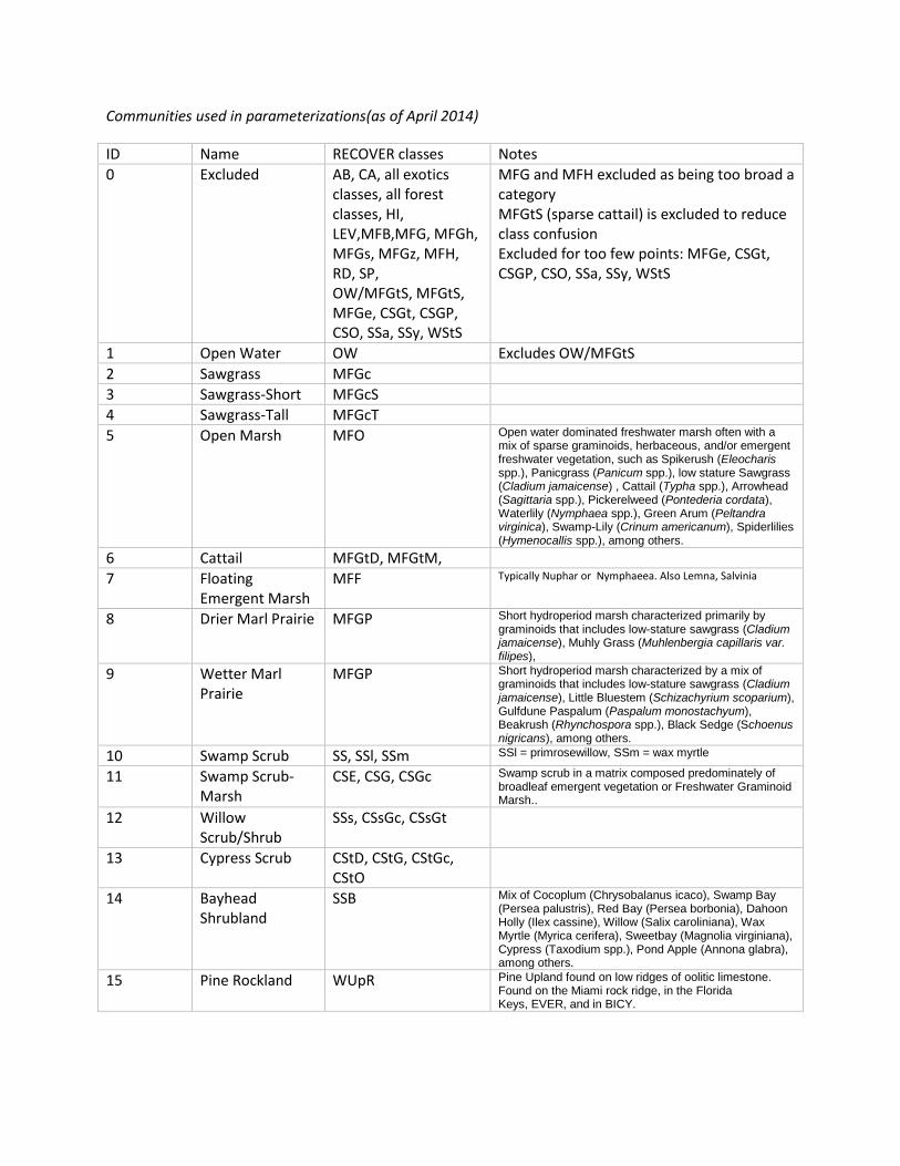
Communities used in parameterizations(as of April 2014)
ID Name RECOVER classes Notes
0 Excluded AB, CA, all exotics classes, all forest classes, HI, LEV,MFB,MFG, MFGh, MFGs, MFGz, MFH, RD, SP, OW/MFGtS, MFGtS, MFGe, CSGt, CSGP, CSO, SSa, SSy, WStS
MFG and MFH excluded as being too broad a category MFGtS (sparse cattail) is excluded to reduce class confusion Excluded for too few points: MFGe, CSGt, CSGP, CSO, SSa, SSy, WStS
1 Open Water OW Excludes OW/MFGtS
2 Sawgrass MFGc
3 Sawgrass-Short MFGcS
4 Sawgrass-Tall MFGcT
5 Open Marsh MFO Open water dominated freshwater marsh often with a mix of sparse graminoids, herbaceous, and/or emergent freshwater vegetation, such as Spikerush (Eleocharis spp.), Panicgrass (Panicum spp.), low stature Sawgrass (Cladium jamaicense) , Cattail (Typha spp.), Arrowhead (Sagittaria spp.), Pickerelweed (Pontederia cordata), Waterlily (Nymphaea spp.), Green Arum (Peltandra virginica), Swamp-Lily (Crinum americanum), Spiderlilies (Hymenocallis spp.), among others.
6 Cattail MFGtD, MFGtM,
7 Floating Emergent Marsh
MFF Typically Nuphar or Nymphaeea. Also Lemna, Salvinia
8 Drier Marl Prairie MFGP Short hydroperiod marsh characterized primarily by graminoids that includes low-stature sawgrass (Cladium jamaicense), Muhly Grass (Muhlenbergia capillaris var. filipes),
9 Wetter Marl Prairie
MFGP Short hydroperiod marsh characterized by a mix of graminoids that includes low-stature sawgrass (Cladium jamaicense), Little Bluestem (Schizachyrium scoparium), Gulfdune Paspalum (Paspalum monostachyum), Beakrush (Rhynchospora spp.), Black Sedge (Schoenus nigricans), among others.
10 Swamp Scrub SS, SSl, SSm SSl = primrosewillow, SSm = wax myrtle
11 Swamp Scrub-Marsh
CSE, CSG, CSGc Swamp scrub in a matrix composed predominately of broadleaf emergent vegetation or Freshwater Graminoid Marsh..
12 Willow Scrub/Shrub
SSs, CSsGc, CSsGt
13 Cypress Scrub CStD, CStG, CStGc, CStO
14 Bayhead Shrubland
SSB Mix of Cocoplum (Chrysobalanus icaco), Swamp Bay (Persea palustris), Red Bay (Persea borbonia), Dahoon Holly (Ilex cassine), Willow (Salix caroliniana), Wax Myrtle (Myrica cerifera), Sweetbay (Magnolia virginiana), Cypress (Taxodium spp.), Pond Apple (Annona glabra), among others.
15 Pine Rockland
WUpR Pine Upland found on low ridges of oolitic limestone. Found on the Miami rock ridge, in the Florida Keys, EVER, and in BICY.

1
Leonard Pearlstine
Steve Friedman
Matthew Supernaw
Ecological Modeling Team
South Florida Natural Resources Center
Everglades National Park
July 30, 2011
Everglades Landscape Vegetation Succession Model (ELVeS)
Ecological and Design Document:
Freshwater Marsh & Prairie Component version 1.1

2
TABLE OF CONTENTS Acknowledgements .............................................................................................................................................................. 4
Glossary of Acronyms .......................................................................................................................................................... 5
Introduction ............................................................................................................................................................................. 6
Section I - ELVeS Model Framework ............................................................................................................................. 7
Model Input and Preprocessing .................................................................................................................................. 9
Hydrologic Parameters .............................................................................................................................................. 9
Soil – Nutrient Parameters ..................................................................................................................................... 10
Fire and Storm Parameters .................................................................................................................................... 12
Salinity Parameters ................................................................................................................................................... 12
Spatial Domain and Resolution ............................................................................................................................ 12
Model Calculations ......................................................................................................................................................... 13
Model Output .................................................................................................................................................................... 14
Section II - Freshwater Marsh Component of ELVeS ............................................................................................ 15
Freshwater Marsh & Wet Prairie Literature Review ....................................................................................... 16
Methods .............................................................................................................................................................................. 24
Vegetation Classification And Base Map ............................................................................................................ 24
Parameterization of Freshwater Marsh & Wet Prairie Component of ELVeS ......................................... 26
Temporal Lag Implementation ................................................................................................................................. 30
Mapped Probability Results ....................................................................................................................................... 32
Calibration and Validation .......................................................................................................................................... 33
Definitions ..................................................................................................................................................................... 33
Calibration .................................................................................................................................................................... 33
Validations .................................................................................................................................................................... 35
Limitations .......................................................................................................................................................................... 36
Future Directions ............................................................................................................................................................ 37

3
Literature Cited .................................................................................................................................................................... 39
List of Tables .......................................................................................................................................................................... 48
List of Figures ........................................................................................................................................................................ 69
Appendix A. Hydrologic metrics calculated from the EDEN data archive ................................................... 90
Appendix B. Hydrologic metrics comparison of the literature by Richards and Gann (2008) ........... 93
Appendix C. Histograms of the relative frequency of occurrence of binned values for each of the
modeled variables within each of the mapped fresh Water marsh and Wet Prairie vegetation
classes. ................................................................................................................................................................................... 107
Appendix D. Recode tables for cross-walking RECOVER vegetation mapping with the Florida GAP
vegetation classification. ............................................................................................................................................... 115
Appendix E. Vegetation recoding and cross walks for south Florida GAP and the RECOVER
vegetation maps. ............................................................................................................................................................... 123
Comments and Questions on this report.
Contact [email protected]
Suggested Citation: Pearlstine, L., S. Friedman, M. Supernaw. 2011. Everglades Landscape Vegetation Succession Model (ELVeS) Ecological and Design Document: Freshwater Marsh & Prairie Component version 1.1. South Florida Natural Resources Center, Everglades National Park, National Park Service, Homestead, Florida. 128 pp.

4
ACKNOWLEDGEMENTS We sincerely thank the following individuals for the time and advice they have offered in
workshops and individually. Their participation is deeply appreciated. We look forward to
their continued involvement and encourage the participation of others.
Susan Bell
Laura Brandt
Carlos Coronado
Don DeAngelis
Mike Duever
Vic Engel
Robert Fennema
Jim Fourqurean
Daniel Gann
Andrew Gottlieb
Marguerite Koch
Alicia LoGalbo
Agnes McLean
Susan Newman
Caroline Noble
Todd Osborne
Dianne Owen
Bill Perry
Jed Redwine
Jennifer Richards
Mike Ross
Jimi Sadle
Jay Sah
Len Scinto
Tom Smith
Leo Sternberg
Maya Vaidya
John Volin
James Watling
Paul Wetzel
Christa Zweig
University of South Florida
U.S. Fish and Wildlife Service
South Florida Water Management District
U.S. Geological Survey
South Florida Water Management District
National Park Service
National Park Service
Florida International University
Florida International University
South Florida Water Management District
Florida Atlantic University
National Park Service
National Park Service
South Florida Water Management District
National Park Service
University of Florida
Florida Atlantic University
National Park Service
U.S. Army Corps of Engineers
Florida International University
Florida International University
National Park Service
Florida International University
Florida International University
U.S. Geological Survey
University of Miami
National Park Service
University of Connecticut
University of Florida
Smith College
University of Florida

5
GLOSSARY OF ACRONYMS
ANPP Above ground net primary production
ATLSS Across Trophic Level System Simulation
BCNP Big Cypress National Preserve
BD Bulk density
CERP Comprehensive Everglades Restoration Plan
CSSS Cape Sable seaside sparrow
EDEN Everglades Depth Estimation Network
ELM Everglades Landscape Model
ELVeS Everglades Landscape Vegetation Succession model
ENP Everglades National Park
EPA Environmental Protection Agency
GAP Gap Analysis Program
LOI Loss on ignition
NSM Natural Systems Model
RECOVER Restoration Coordination & Verification
R-EMAP Regional Environmental Monitoring and Assessment Program
RSM Regional Simulation Model
SFWMD South Florida Water Management District
SFWMM South Florida Water Management Model
TaRSE Transport and Reaction Simulation Engine
TC Total carbon
TIP Total inorganic phosphorus
TN Total nitrogen
TM Total magnesium
TP Total phosphorus
WCA Water Conservation Area

6
INTRODUCTION
The Everglades Landscape Vegetation Succession model (ELVeS) is a spatially explicit
simulation of vegetation community dynamics over time in response to changes in
environmental conditions. The model uses empirically based probability functions to define the
realized niche space of vegetation communities. Temporal lags in response to changing
environmental conditions are accounted for in the model. ELVeS version 1.1 simulates
Everglades freshwater marsh and prairie community response to hydrologic and soil properties.
Subsequent versions of ELVeS are planned to include a larger suite of vegetation communities
and responses to disturbances such as fire and storms. Figure 1 illustrates the Everglades spatial
domain for ELVeS parameterization including the Water Conservation Areas (WCAs) and
Everglades National Park (ENP).
ELVeS has been developed to provide scientists, planners, and decision makers a simulation
tool for Comprehensive Everglades Restoration Project (CERP) landscape-scale analysis,
planning, and decision making. The model is also intended for integration with wildlife models
to provide a temporally dynamic vegetation input layer. We anticipate that ELVeS will consider
a suite of vegetation communities within the CERP planning domain that span a wide suite of
environmental conditions from seagrass communities, freshwater marshes, mangroves, saline
prairies, and tropical and temperate hammocks to upland pine forests (Figure 1). Eleven of the
communities are in the freshwater marsh and wet prairie component described in this report. Of
the 11 communities, three are too broadly defined to effectively model, leaving eight freshwater
marsh and wet prairie classes parameterized in this version of ELVeS (Figure 2).
ELVeS v.1.1 is the first iteration of a model design and parameterization process that relies on
feedback from the knowledge and experience of the larger scientific community to continually
improve the model’s capabilities and performance. To encourage that process, we attempt to be
explicit in discussing methods, presenting validation trials, acknowledging current limitations,
and proposing potential future directions. The iterative design process is also explicitly
implemented in ELVeS program coding with an open graphical user interface design that
allows easy modification to the variable selected and their parameterization (ELVeS User’s
Guide, Supernaw et al. 2011). User and developer interaction to further ELVeS development is
also encouraged by web distribution of the application and its open source code
(www.SimGlades.org).
ELVeS v.1.1 treats each of the major vegetation communities and community drivers as user-
accessible components of the model. In future versions, we anticipate ELVeS will integrate
vegetation succession components for seagrasses, mangroves, saline prairies, freshwater
marshes, hammocks, tree islands, cypress, and pine forests in a single simulation model.
Incorporating the coastal system communities in a general Everglades vegetation succession

7
model along with inland marsh and terrestrial community types represents a fundamental
progression of vegetation succession modeling for this diverse ecosystem. ELVeS is designed
with the capacity to integrate future modules for climate change, hurricanes, and fire scenarios,
providing the opportunity to explore potential habitat modifications for estuarine, freshwater,
and coastal vegetation, and their effects on wildlife communities.
Design considerations were developed following initial open discussion workshops that were
conducted in 2009 and 2010 addressing four broad categories of 1) freshwater marshes, 2)
coastal and estuarine communities, 3) tree islands, and 4) forest communities. Participants of
these workshops represented university scientists, Restoration Coordination and Verification
(RECOVER) team members, and government scientists. Discussions during these meetings
considered a wide variety of topics. For example, meeting participants were asked to consider
and make recommendations for a baseline Everglades vegetation map, assessment of known
ecological drivers, and reasons and opportunities to develop new vegetation succession metrics.
Open discussions were held to inform participants of the final selected critical ecological
drivers, approaches to parameterizing drivers, and the format of the model outcomes. Additional
considerations related to the availability of regional data sets limited ELVeS v.1.1 development.
For example, we had to use static multivariate soil data layers even though multi-temporal data
layers would be much more desirable. ELVeS has been designed to be easily modified,
recognizing a need for flexibility that promotes the integration of new data layers as they
become available.
This report details the progressive development of the freshwater marsh component of ELVeS
and the ecological basis for the relationships and rules reflected in the model. Section I of the
report provides a broad overview of the ELVeS modeling framework including the model
description, data integration, data processing, and simulation solutions. Section II follows with a
description of the application of the ELVeS framework to Everglades freshwater marsh
communities. Methods of analyses of empirical ecological data within the modeled domain and
selection of principal hydrologic and soil biogeochemical processes in the freshwater
communities are described. The methods are followed by simulation results, notes on model
limitations, and potential future directions of model development.
SECTION I - ELVES MODEL FRAMEWORK
ELVeS is a spatially explicit cell-based probability model designed to predict the likelihood of
specific vegetation communities given a set of specific environmental conditions. The
underlying structure of the model is the geographic spatial domain represented by a regular grid
of cells. Ecological driver state conditions are calculated for each cell in order to calculate
characteristics of multi-dimensional niche space at each location. Estimated probabilities of

8
vegetation communities occupying the derived realized niche space are then calculated using a
conditional probability based method.
Other spatially explicit vegetation and wildlife models have been formulated following several
alternate methodological procedures similar to ELVeS including gradient percolation and
gradient contact process models (Gastner et al. 2009), agent based models (Topping et al. 2003),
transition-matrix probability models (Perry and Enright 2007), linear regression models (Li et
al. 2003), stochastic individual species models (Mladenoff 2004), and rule-based models
including the Across Trophic Level System Simulation (ATLSS) vegetation succession model
for the Everglades (Duke-Sylvester 2006). All of these models rely on a variation of probability
theory or conditional rule sets as an underlying modeling approach for assigning niche space
conditions and outcomes.
The ATLSS vegetation succession model (Duke-Sylvester 2006) was a pioneering and
innovative approach to the challenge of modeling Everglades freshwater vegetation succession
based on an extensive literature review of vegetation community hydroperiod estimates and fire
disturbance nutrient estimates compiled by Wetzel (2001, 2003) for the ATLSS project
(DeAngelis et al. 2000). Although it was our initial plan to build on and update the existing
ATLSS model, we concluded that was not practical or efficient because the existing code is
difficult to modify and was not built with the modular structure we seek to allow rapid
adaptation to other models and rapid modifications as desired in future iterations. Although the
procedures are conceptually well presented in Scott Duke-Sylvester’s dissertation (Duke-
Sylvester 2006), the code itself is undocumented. Specifically, we sought model modifications
because:
1. There is a considerable amount of new information published after Wetzel’s (2001) report
and development of the ATLSS model. Some of that information is synthesized by the literature
review in this report and by other authors such as Richards and Gann (2008).
2. Using modern, object-oriented programming techniques, standardized methods, and standard
file formats (a) increases model flexibility to future changes, (b) enhances opportunities for
collaborative development, and (c) allows us to more efficiently couple vegetation routines with
specific hydrology models and wildlife/habitat response models.
3. We sought the capacity to model vegetation response to several factors differently, including
hydroperiod, nutrients, and fire. The ATLSS model does not replace vegetation communities if
hydroperiod is within range for that community. ELVeS uses response distributions to consider
the probability for new communities to outcompete existing community when hydrologic or
other parameters are within range, but not optimal for the existing community. Nutrients are a
critical driver, but phosphorus is only considered in the ATLSS model if there is a fire in the
current year. ELVeS treats nutrients in the same way as other parameters defining the niche
space of the community. Dynamic phosphorus modeling is not available in ELVeS v.1.1, but is
planned for future versions in coordination with fire modeling. Fire calibration in the ATLSS

9
model is dependent on historic patterns and proportions of hot and cold fires. Historic trends
have been found not to correlate with current fire activity (Rick Anderson, pers. comm., ENP
2008). Particularly with climate change, we need to consider temperature and precipitation
relationships to those patterns and allow a dynamic change in fire patterns. Fire is not modeled
in ELVeS v.1.1, but it is planned for future versions.
4. To address sea level rise and climate change response in future vegetation succession
modeling, coastal and near-shore coastal vegetation communities need to be incorporated as
well as salinity and climate tolerance responses.
5. A goal in ELVeS design was to provide a model that adapts readily to iterative
experimentation and change. In addition to open source code distribution and the already
mentioned object oriented design, the ELVeS interface permits rapid variable modification
without requiring code changes (ELVeS User’s Guide, Supernaw et al. 2011).
Figure 3 illustrates ELVeS data pre-processing and simulation occurring within five stages: 1)
Data inputs to the model, 2) Pre-processing of input data, 3) Probability calculations, 4)
Temporal lag controls on community succession and 5) Model output. The stages are described
below.
MODEL INPUT AND PREPROCESSING
Planned model inputs originate from one of five primary data domains:
1. hydrology
2. soil biogeochemistry
3. salinity
4. fire
5. storms
HYDROLOGIC PARAMETERS
Hydrologic input data may come from a variety of data sources and modeling output that
provide spatially continuous water depths (e.g., Everglades Depth Estimation Network (EDEN),
South Florida Water Management Model (SFWMM), Natural System Model (NSM), Regional
Simulation Model (RSM), and other hydrologic models). These data are pre-processed to

10
extract a suite of hydrologic metrics (Appendix A) that were evaluated for use in the
classification engine. The utility to extract hydrologic metrics was created in-house, and details
of its use are provided in the HydroMetrics program User’s Guide (SFNRC 2011a).
Numerous hydrologic metrics have been used by investigators working in the Everglades. One
result from this large body of work is a plethora of reports identifying similar hydrologic
metrics such as hydroperiod that are useful in describing vegetation response (Appendix B). The
decision to examine and develop a larger set of derivative hydrologic metrics than those
described in the literature followed from the spring 2010 workshop. It was clear to the
workshop participants that limiting ELVeS parameterizations to the previously developed
parameters would not provide the sufficient analytical information required to enhance
performance of the model. Additional hydrologic metrics, representing different temporal
periodicities and estimates of parameter variability were expected to better quantify ecological
relationships between vegetation communities and hydrologic drivers. This was undertaken
following recommendations that several new metrics in addition to seasonally based wet and
dry periods, and mean annual water depth estimates would enhance examination of critical
relationships between vegetation and the hydrologic environment. Forty-nine hydrologic
metrics were identified (Appendix A) in response to this suggestion. As of this report, water
depth simulations from EDEN (releases as of July 2010) and SFWMM ECB3 v.6.0 daily data
records have been used to calculate annual estimates for each of the 49 metrics. EDEN is an
interpolated water-depth data layer from a water level monitoring network (Liu et al. 2009).
This report uses the daily median water-depth data layers for the period from 2000 to 2010.
SFWMM ECB3 is the existing conditions baseline alternative of the SFWMM covering the
period from 1965 to 2000. Pearson correlations were calculated for the EDEN hydrologic metric
set to aid in reducing the metric set used in modeling by determining degrees of independence
among the metrics (Table 1). The majority of the metrics were determined to be both highly
positively and negatively correlated with one another as expected. Selection of hydrologic
metrics for use in ELVeS was governed by two criteria; 1) maximizing separability and 2)
reducing correlation of vegetation community classes. Selection of parameters based on low
correlation scores reduces the multi-dimensional niche space to the fewest number of
independent metrics, thereby making the model more efficient in defining a niche space.
However, some correlated metrics still aided in achieving maximum separation of communities.
The vegetation community relationships with the metrics are modeled simplifications of
multidimensional environmental gradients. Community composition is often overlapping in
these modeled niche spaces.
SOIL – NUTRIENT PARAMETERS
11
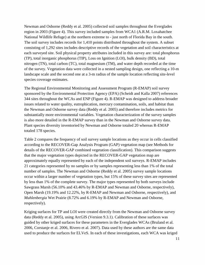
Newman and Osborne (Reddy et al. 2005) collected soil samples throughout the Everglades
region in 2003 (Figure 4). This survey included samples from WCA1 (A.R.M. Loxahatchee
National Wildlife Refuge) at the northern extreme to - just north of Florida Bay in the south.
The soil survey includes records for 1,410 points distributed throughout the system. A subset
consisting of 1,292 sites includes descriptive records of the vegetation and soil characteristics at
each surveyed site. Soil physical property attributes included in this survey are: total phosphorus
(TP), total inorganic phosphorus (TIP), Loss on Ignition (LOI), bulk density (BD), total
nitrogen (TN), total carbon (TC), total magnesium (TM), and water depth recorded at the time
of the survey. Vegetation data were collected in a nested sampling design, one reflecting a 10-m
landscape scale and the second one at a 3-m radius of the sample location reflecting site-level
species coverage estimates.
The Regional Environmental Monitoring and Assessment Program (R-EMAP) soil survey
sponsored by the Environmental Protection Agency (EPA) (Scheidt and Kalla 2007) references
344 sites throughout the WCAs and ENP (Figure 4). R-EMAP was designed to address broader
issues related to water quality, eutrophication, mercury contamination, soils, and habitat than
the Newman and Osborne survey data (Reddy et al. 2005) and therefore includes metrics for
substantially more environmental variables. Vegetation characterization of the survey samples
is also more detailed in the R-EMAP survey than in the Newman and Osborne survey data.
Plant species diversity inventoried by Newman and Osborne totaled 20 whereas R-EMAP
totaled 178 species.
Table 2 compares the frequency of soil survey sample locations as they occur in cells classified
according to the RECOVER-Gap Analysis Program (GAP) vegetation map (see Methods for
details of the RECOVER-GAP combined vegetation classification). This comparison suggests
that the major vegetation types depicted in the RECOVER-GAP vegetation map are
approximately equally represented by each of the independent soil surveys. R-EMAP includes
21 categories represented by no samples or by samples representing less than 1% of the total
number of samples. The Newman and Osborne (Reddy et al. 2005) survey sample locations
occur within a larger number of vegetation types, but 15% of these survey sites are represented
by less than 1% of the complete survey. The major types represented by both surveys include
Sawgrass Marsh (56.10% and 43.46% by R-EMAP and Newman and Osborne, respectively),
Open Marsh (19.19% and 12.22%, by R-EMAP and Newman and Osborne, respectively), and
Muhlenbergia Wet Prairie (8.72% and 6.19% by R-EMAP and Newman and Osborne,
respectively).
Kriging surfaces for TP and LOI were created directly from the Newman and Osborne survey
data (Reddy et al. 2005), using ArcGIS (Version 9.3.1). Calibration of these surfaces was
guided by other kriged surfaces for these parameters in the Everglades WCAs (Bruland et al.
2006, Corstanje et al. 2006, Rivero et al. 2007). Data used by these authors are the same data
used to produce the surfaces for ELVeS. In each of these investigations, each WCA was kriged

12
independently. The surfaces developed for ELVeS used data from the complete survey,
including ENP, but, in this first iteration of the model, disregarded canals, roads, and other
infrastructure that divide the Everglades into unique water impoundment areas.
Parameterization values for the kriged surfaces developed for ELVeS are reported in Table 3.
FIRE AND STORM PARAMETERS
Fires and storms are not yet incorporated in this model. Because these disturbance regimes are
important in Everglades ecology we anticipate they will be included in future versions of the
model.
SALINITY PARAMETERS
Although the saline community modeling component is also not presented in this report, it is
useful to note that Antlfinger and Dunn (1979) developed a classification scheme integrating
frequency of flooding and interstitial salinity to discriminate saline prairie vegetation. ELVeS
will examine these classifications and a broader literature base for use in the mangrove and
saline prairie/hardwood zonation areas. Their classification integrates frequency of flooding and
interstitial salinity to discriminate five communities (Rushes (Juncus) – Sea Oxeyes (Borrichia),
Glassworts (Salicornina) – Saltworts (Batis), Salt Flats, Cord Grasses (Spartina), and tidal
creeks) along a saline to freshwater gradient. Two modeling efforts Teh et al. (2008) and Wang
et al. (2007) address vegetation dynamics associated with saline water intrusion and salinity
diffusion in coastal Florida environments. These models may provide a framework for our
modeling design consideration and sea level rise assessments for coastal regions of the
Everglades. Sea level rise is potentially the most important global change factor that will
influence the distribution of the mangrove – saline prairie and the mangrove – hardwood ecotone
boundary. Flooding by increasing sea level and changes in the soil salinity concentrations will be
directly influenced.
SPATIAL DOMAIN AND RESOLUTION
Parameters for each of the input data layers are maintained in NetCDF files as spatially explicit,
geo-referenced information. ELVeS classifies vegetation distribution patterns within each of the
WCAs, and ENP (Figure 2). Inclusion of Big Cypress National Preserve (BCNP) is anticipated

13
in future releases as forested communities are included in the model and as better continuous
data layers become available for the preserve. Templates or geographic masks can be defined in
a pre-processing step or as post-processing to focus the model output on a smaller isolated zone
such as Taylor Slough in ENP, or a single model cell.
The modeling resolution of ELVeS is unrestricted and dependent only on the resolution of input
data sources. For example, EDEN hydrologic data are geo-referenced in a 400 x 400-m
resolution regular grid and output will match the EDEN grid when EDEN is used as the input
hydrologic layer. The model is flexible and can accept input data from any CF-compliant
NetCDF format regular grids, including CERP-compliant NetCDF, such as the SFWMM (with
either 2 x 2-mile or 500 x 500-m resolution) or potentially even grids with finer resolutions for
local modeling. The ability to accept variable resolution mesh input data such as the RSM is
anticipated in the near future.
MODEL CALCULATIONS
ELVeS operates as a raster at 400-m resolution when using the EDEN grid and hydrology.
When the SFWMM is used for hydrologic input, the Delaney triangulation method was used to
interpolate the SFWMM grid and hydrology to a 500-m resolution. Every grid cell processes
the hydrologic, soils, and nutrient information on a yearly time step to define an ecological
niche for each year of the simulation. Each of the input data files is stored independently as a
NetCDF file that is accessed during the data pre-processing stage. Model output is developed
for every modeled cell. When other hydrologic models are used, the spatial domain (number of
cells and spatial resolution) changes relative to the selected hydrologic model.
Every cell in the raster is parameterized to characterize a multi-dimensional environmental
gradient space. Instantaneous probability scores for the vegetation types are calculated by
examining the ecological drivers on a cell-by-cell basis. That is, for each environmental
variable (or driver), a distribution function has been established for the estimated probability of
occurrence for each of the vegetation communities. The model uses the joint probability
distribution functions to classify the likelihood for each vegetation community within individual
cells during a model run. Vegetation types with the highest-ranking instantaneous probability
score are evaluated against the current community and temporal lags in community transition to
produce a final vegetation map. Instantaneous probabilities refer to the probability of a
vegetation type occurring in a cell, given the environmental conditions in the current year.
Temporal lags control how quickly an existing community will be replaced when a different
community has a higher probability of being at the location. The equations of these procedures
are presented in more detail below for the freshwater marsh component. Because ELVeS is

14
typically expected to operate at resolutions of 400 to 500 m, the influence of spatial neighbors
on community succession was assumed to be minimal and was not modeled.
The vegetation community with the highest joint probability is defined as the dominant type
within specific cells. Dominance in the current version of the ELVeS model doesn’t address the
issue of assigning a ―winning‖ vegetation type when its probability, for example is 27% and the
second highest ranking type has a 26% probability, an insignificant difference. However,
probability estimates for each vegetation community are stored regardless of whether it is the
highest-ranking probability, allowing users to assess possible ecotonal conditions or for post-
processing applications.
The final vegetation community predicted to occur in each cell is the probability of occurrence
when considering temporal lags. This result is a stochastic simulation that assigns an increasing
probability that the community will be replaced when there is an increasing number of years
with low instantaneous probability that the current vegetation community should be dominant.
MODEL OUTPUT
The ELVeS model creates several layers of projected, spatially explicit mapped output that
allow the user to examine the individual probabilities that result in the final mapped
classification. Those layers are:
1. Conditional probabilities of occurrence for each of the vegetation communities, given each
input variable independently
e.g., for each grid cell: P(i| j)
where i = each of the vegetation communities and j = each of the input variables
2. Joint instantaneous probabilities of occurrence of each of the vegetation communities when
the input variable results are combined as a geometric mean
e.g., for each grid cell: P(i) = (P(i| j1) × P(i| j2) × P(i| j3) … × P(i| jn))1/n
3. The dominant instantaneous probability predicted vegetation community
e.g., for each grid cell: for the set of community instantaneous probabilities (P(i)) select the
community with the highest probability.
4. The secondary instantaneous probability predicted vegetation community

15
e.g., for each grid cell: for the set of community instantaneous probabilities (P(i)) select the
community with the second highest probability.
5. Temporal lagged vegetation community response.
e.g., the dominant vegetation community after simulation of temporal lags.
Because the intermediate model outputs for conditional probabilities and joint instantaneous
probabilities are retained, the investigator can reconstruct the communities at each grid cell in
increasing detail as desired. The distribution of probabilities for each community in the grid cell
is available as well as the contribution that each metric contributes to that probability. Temporal
lags associated with community change are integrated in the modeling and predicted community
probabilities reflect this dynamic.
SECTION II - FRESHWATER MARSH COMPONENT OF ELVES
This report focuses on the freshwater marsh component of ELVeS v.1.1. Forest communities
and coastal saline wetland communities are planned for incorporation into ELVeS in future
versions. Background information for the freshwater marsh component of ELVeS comes from a
variety of sources including published literature in ecological journals, professional technical
reports, and decisions based on the series of species expert workshops that were conducted to
design the model. A February 2009 workshop led to the initial parameterization of ELVeS.
Results based on this initial development work were presented to freshwater marsh workshop
participants in March 2010. The outcome of these reviews and discussions was recognition of
the need for additional parameters and further analyses to improve model performance.
Parameters used to model the freshwater marsh had to come from available, spatially
continuous data layers or from data layers that could be readily constructed. Two criteria for
parameter selection are reducing correlation and maximizing separability of the marsh
communities. This documentation examines the probability of occurrence for 11 freshwater
marsh communities (Spikerush, Graminoid Marsh, Willow, Cattail, Open Marsh, Floating
Emergent Marsh, Muhlenbergia Wet Prairie, Mixed Marl Wet Prairie, Sawgrass, Herbaceous
Marsh, and Open Water) matching community descriptions from the RECOVER classification
scheme (Rutchey et al. 2006)). Of the 11 classes investigated, eight are modeled in this version
of ELVeS as discussed below.
16
FRESHWATER MARSH & WET PRAIRIE LITERATURE REVIEW
We conducted a literature review to identify specific environmental drivers that affect
vegetation succession in the Everglades. Broad ecotonal overlap among communities can result
in investigators reporting different environmental responses to similarly labeled vegetation
classes. The problem of possibly comparing unlike communities is exacerbated by
inconsistencies in nomenclature such as in references to ―wet prairie.‖ Conclusions drawn
between the freshwater communities modeled on the RECOVER classification scheme and
information identified in the literature should be based on firm knowledge of the methods and
nomenclature used by the referenced investigator.
This literature review, in concert with workshops and discussions with local investigators, set
the stage for modeling Everglades graminoid communities and was central in guiding our
approach to developing metrics for vegetation response. The Methods section of this report
details when relationships identified in the literature review were used directly in the ELVeS
model. Perhaps most importantly, however, the literature served to inform our understanding of
how and why species and communities segregate on the landscape. Ultimately, this background
provided a basis for developing a multivariate statistical assessment of the metrics used to
parameterize the model.
The term ―wet prairies‖ can refer to short-term or longer-term hydroperiod locations in the
Everglades. Unfortunately, this term is used indiscriminately throughout Everglades science
literature obfuscating discussion of two unique communities: deeper-water marsh communities
underlain by peat common in the central and northern portions of the system and southern
Everglades marl communities that occur on calcitic pinnacle rock (Lodge 2010). Long-term
hydroperiod wet prairies are dominated by spikerush (Eleocharis spp.) and occupy three times
as much area as do the short-term hydroperiod prairies (Rutchey et al. 2006). Short-term
hydroperiod wet prairies occur in ENP and in the adjacent BCNP on marl substrates and are
dominated by Gulf muhly (Muhlenbergia capillaris var. Filipes) or mixed graminoids.
Vegetation composition and structural patterns in wet prairie settings varies responding to a
combination of hydropattern characteristics (Armentano et al. 2006, Childers et al. 2006), but
also to substrate (peat vs. marl) and phosphorus distribution (Doren et al. 1997, Childers et al.
2006). Hydropattern in the Everglades has been considered as a principal factor in virtually all
ecological dynamics for wet prairies, marsh, and slough communities (Appendix B). Each of
these components has a significant bearing on vegetation dynamics. Hydroperiod is often cited
as a primary driver responsible for vegetation distribution patterns. As will be illustrated in this
report, hydroperiod is only one of several hydrologic drivers that should be considered when
modeling vegetation dynamics and distribution patterns. In fact, the analysis conducted in
support of the model development demonstrates that discontinuous hydroperiod does not
provide sufficient ecological separability among vegetation communities in comparison to other

17
hydrologic metrics (See Methods and Appendix C). Ross et al. (2003a), Richards and Gann
(2008), and Gann and Richards (2009), for example, identified water depth, length of draw-
down periods, and variability of mean annual water depth among the critical drivers of
vegetation dynamics.
Different authors have used a variety of terms to identify marl wet prairie vegetation (U.S. Fish
and Wildlife Service 1999). Synonyms include Marl Prairie, Short Sawgrass Prairie,
Muhlenbergia Prairie, Mixed Grass/Sedge Prairie, and Rocky Glades Prairie (Olmsted et al.
1980, Kushlan 1990, Olmsted and Armentano 1997, Davis et al. 2005, Bernhardt and Willard
2006, Sah et al. 2006). Dominant species include Gulf muhly and sawgrass (Cladium
jamaicense). Subdominant species include black sedge (Schoenus nigricans), arrowfeather
threeawn (Aristida purpurascens), Florida little bluestem (Schizachyrium rhizomatum), and love
grass (Eragrostis elliottii). Marl prairies are situated in slightly higher (30 cm or less) elevated
positions east and west of Shark River Slough, ENP. Historically, these areas experienced
inundation periods lasting from 2 to 9 months and supported different dominant vegetation.
Following the development of the Central and Southern Florida Project, this pattern reversed
with dry downs lasting an average of 9 months (Van Lent et al. 1993, Fennema et al. 1994).
Armentano et al. (2006) suggested inundation periods of 2 to 4 months with occasional periods
of 6 months in the southern coastal wet prairies. History seldom documents complete biological
records and such is the case of the role of Gulf muhly in the southern Everglades marshes.
Armentano et al. (2006) raises concern that the substantial presence of Gulf muhly in marl
prairies is potentially an artifact of recent hydrologic mismanagement and fire incidence. Lower
water depths and short hydroperiods are conducive to development of Gulf muhly dominance.
Greater water depths and longer inundation periods will alternatively favor other species, such
as sawgrass and or spikerush (in the absence of elevated phosphorus). Marl prairie is the
primary habitat for the Cape Sable seaside sparrow (CSSS) (Ammodramus maritimus mirabilis).
Field surveys of nest site occupancy have demonstrated different preferences for marl plant
communities exhibiting slightly drier conditions and shorter hydroperiods as highlighted in
Table 4.
Nott et al. (1998) investigated water management histories in the marl prairies adjacent to Shark
River and Taylor Slough to improve understanding of CSSS population dynamics. Their
assessment identified an association between the management of water as a principal agent
responsible for major population declines in this endangered species. Marl prairies west of
Shark River Slough were determined to be ―too wet‖ during critical breeding seasons and
prairies east of Taylor Slough were both ―too wet and too dry‖ (Nott et al. 1998). Gulf muhly, a
dominant species in the short-hydroperiod marl communities, lost its competitive advantage to
sawgrass when the hydroperiod was extended. Perhaps as a secondary factor, community
trajectory is also influenced by periphyton dynamics and its spread in sloughs. Above ground
net primary production (ANPP) estimates of periphyton in the Everglades were examined by
18
Ewe et al. (2006). Estimates of periphyton productivity reported by these investigators were
demonstrated to be influenced by water levels and residence times. Overall, periphyton ANPP
estimates in Taylor Slough and Shark River Slough represent some of the highest and most
variable in the world (Ewe et al. 2006). Long-hydroperiod (greater than 210 days) and short-
hydroperiod (60-210 days) periphyton mats differ in a number of critical ecological
characteristics including biodiversity and magnitude of dry and ash-free weight. Development
of biomass is greater in short-hydroperiod marshes compared to long-hydroperiod deeper
marshes. These lower trophic order ecological characteristics are important for higher order
ecosystem processes in nutrient biogeochemistry exchange and macrophyte productivity. Nott
et al. (1998) proposed a conceptual model that describes an interaction between hydroperiods,
periphyton, Gulf muhly, and sawgrass. They suggest that longer hydroperiods in the marl
prairies will initiate greater periphyton productivity resulting in larger, thicker mats that can
dislodge and float. Shading of the submerged macrophytes may reduce the ability of the
submerged plant species to survive inundation. Sawgrass culms can penetrate these mats while
Gulf muhly culms cannot. As the hydroperiod decreases, Gulf muhly would normally become
reestablished as the dominant species. These authors further suggest that these mats may be
large and occupy large patches. If this mechanism is correct, local scale patch dynamics and
local-scale successional trajectories could be mediated by these interactions. The primary
trajectories of marl prairies, discussed in the literature, revolve around the hydrologic factors.
Other factors are also critical. An unambiguous characterization of the hydroperiod in this
system is seldom agreed upon in the literature. Some authors as indicated above suggest a 2- to
9-month (Davis et al. 2005) hydroperiod while others suggest 3 – 7 months (Nott et al. 1998).
Deriving a strict definition for all practical purposes is not feasible because representative
species have narrower or wide tolerances and many of the species are also present in long-
hydroperiod marsh settings. Lower water tables and shorter hydroperiods may increase the
likelihood of conversion to a more woody vegetation type. For example, invasion by the
natives, wax myrtle (Myrica cerifera) and willow (Salix caroliniana), and exotic tree and shrub
species such as melaleuca and Brazilian pepper-tree (Melaleuca quinquenervia and Schinus
terebinthifolius, respectively) could represent a potential for change in this subsystem.
Change in short-hydroperiod marsh vegetation was documented by Ross et al. (2003a) and
Armentano et al. (2006). Water management delivery to the Taylor Slough elevated marl
marshes changed over a 30+ year time span as new infrastructure was constructed or removed.
Vegetation response patterns were directly associated with the hydrologic dynamics that these
changes caused. Sites that initially supported Gulf muhly became wetter and transitioned
between sawgrass and spikerush communities. Similarly, sites that became drier trended from
spikerush to sawgrass and from sawgrass to Gulf muhly. Although uniform change was not
observed, the overall direction of change was from drier to wetter conditions. In addition to the
three dominant marl species, 26 subordinate species were identified along the five transects
during the survey period. Wetter conditions reduced species richness on transects (Ross et al.
19
2003a, Armentano et al. 2006). Change in species abundance may occur rather quickly, within
3- to 4-year time periods trending toward either longer- or shorter-hydroperiod species given
increasing or decreasing hydroperiod trends. One of the major findings from Ross (2003a,
2003b), however, was that changes in community composition could not easily be associated
with a discernible temporal lag period. Hotaling et al. (2009) and Zwieg and Kitchens (2008,
2009) suggest lag periods as long as 4 years may be critical determinants of vegetation
community response in the wet prairies of WCA3A. Armentano et al. (2006) reported that
changes in species dominance (Gulf muhly to sawgrass and sawgrass to spikerush) in Taylor
Slough was detectable within 3 to 4 years and continued for an additional 3 years following
changes linked to the S332 and S332D water management structures at the head of Taylor
Slough. Childers et al. (2003) resurveyed transects, first reported by Doren et al. (1997) in
WCA1, WCA2, and WCA3, finding significant changes in composition and species richness
and linked these changes to nutrient concentrations. Given that observed changes in Taylor
Slough were inconsistent and occurred across fine topographic scales, and that various authors
report different estimated temporal lags, extrapolating change dynamic behavior reported from
one area of the system to a broader geographic domain of the Everglades remains a difficult
process.
Hydroperiod alone only partially explains how vegetation communities are distributed in wet
prairies and sloughs. A generalized realization of the community distribution pattern positions
bayhead swamps and tall sawgrass communities in shorter hydroperiod zones near sparse
sawgrass with slightly longer hydroperiods followed ultimately by spikerush communities in the
longest marsh hydroperiod settings (Ross et al. 2003a). Spikerush and sparse sawgrass
communities according to this gradient occupy sites with average annual water depths of 25 cm
lasting for approximately 9 months. Tall sawgrass sites may be inundated for 6 – 10 months,
and bayhead swamps for 2 – 6 months (Ross et al. 2003a). Earlier investigations (Olmsted and
Armentano 1997, Busch et al. 2004) that examined relationships between water depths and
hydroperiod also reported significant relationships between vegetation distribution patterns and
the interaction between hydroperiod length and water depth.
Ross et al. (2003a) quantified this relationship, suggesting that a narrow threshold of 5- to 10-
cm change in water depth or a 10- to 60-day hydroperiod change can alter the dominance of
vegetation types within specific geographic settings. Brandt (2006) combined data from
Richardson et al. (1990) and Jordan (1996) to surface elevation differences among vegetation
communities in WCA1. She reports surface elevation differences of 10 cm between slough and
wet prairie (primarily spikerush), 19 cm between slough and sawgrass, and 5 cm between
sawgrass and brush/shrub. Given the fine spatial- and temporal-scale relationships between
these hydrologic factors, regional models of vegetation dynamics need to account for each of
these as primary drivers of change.
20
Childers et al. (2006) investigated biomass response patterns of sawgrass and spikerush in the
Taylor Slough region to hydroperiod and salinity fluctuations. Using a non-destructive biomass
sampling technique and repeated measures analysis of variance, they were able to identify
temporal pattern differences in sawgrass and spikerush development. Spikerush is typically
associated with longer hydroperiods than sawgrass. Water management is likely to influence the
stem density and biomass of both of these indicator species. Longer-hydroperiod conditions
favor spikerush while shorter-hydroperiod conditions will shift competitive advantages to
sawgrass and other shorter-hydroperiod preference species (Childers et al. 2006). Increasing
freshwater volumes across Taylor and Shark River Sloughs will influence the vegetation
dynamics predictably; in the absence of elevated phosphorus, longer hydroperiods will favor
species such as spikerush and other long-hydroperiod preference species.
Shorter hydroperiods may exacerbate the frequency of wildfire. However, short-hydroperiod
plant species tend to increase their abundance when the hydroperiod conditions remain stable
for a few years. Short-hydroperiod species include wand goldenrod (Solidago stricta)
(hydroperiod length in days = 138), cypress panicgrass (Dichanthelium dichotomum) (165),
Florida little bluestem (170), erect centella (Centella erecta) (173), and frogfruit (Phyla
nodiflora) (178). In contrast, love grass (224) and bluejoint panicgrass (Panicum tenerum) (232)
are long-hydroperiod species (Ross et al. 2003b). Hydroperiod optima were derived by
examining the weighted averaging regressions and observed average hydroperiods where the
species occurred weighted by their abundances at 91 locations in Taylor Slough (Ross et al.
2003b) . Finally, species tolerance was estimated as the weighted standard deviation of
hydroperiods.
Fire frequency and intensity in marl prairies influences vegetation dynamics. Post-fire biomass
(cover) recovery occurs rapidly. Gulf muhly biomass (cover) following the Mustang Corner
Fire of 2008 was equivalent to or greater than pre-burn levels within 6 months of the fire (Rick
Anderson, ENP, pers. comm., 2008). Herndon and Taylor (1986) assessed vegetation biomass
recovery 1-, 2-, and 3- years after burns in the ENP boundary zone. They reported that live fuel
recovery reached 90% of its pre-burn volume within the first year following fires and that
biomass accumulation continued for two years (Herndon and Taylor 1986). Liu et al. (2010)
characterized cattail (Typha spp.) and sawgrass dynamics from a physiological basis following
prescribed burn experiments conducted in WCA2. Cattail is physiologically and
morphologically better adapted for rapid uptake of phosphorus than is sawgrass due to
photosynthesis rate differences and root growth strategies (Liu et al. 2010).
Site differences between sparse, short sawgrass and tall sawgrass sites are linked to
environmental factors with hydropattern and soil depth being among the most critical. The
relationship may represent a significant controlling factor in the spatial distribution patterns of
tall sawgrass, sparse sawgrass, and spikerush communities. Ross et al. (2003a) investigated
relationships between hydropattern, soil depths, mean water depths, and maximum water depths

21
in Northeast Shark Slough, Central Shark Slough, and Southern Shark Slough along five
transects transverse to Shark River Slough. Results, based on a series of ordinations, Analysis of
Similarity, and Mantel tests indicate that local hydrologic conditions explained differences in
the spatial distribution patterns of sparse sawgrass, spikerush, and tall sawgrass communities.
The dense tall sawgrass communities are linked to deeper soils, a potential consequence of
biomass accumulation and decomposition rates and greater resistance to surface sheet flows.
Spikerush, a species with substantially lower biomass accumulation rates and less resistance to
flow, was associated with shallow soil depths in Southern Shark Slough (Ross et al. 2003a).
Hydropatterns in which deeper stage conditions occur enhance the likelihood for tall sawgrass
development in portions of Shark River Slough. Patterns and associations of soil depth and
vegetation are not globally consistent (Ross et al. 2003a).
Slough, wet prairie, and ridge communities are a continuum in which hydroperiod, depth,
duration of inundation, flow, resilience to water chemistry, and upper soil (0-10 cm) phosphorus
concentrations are pivotal to the structure, state change, and sustainability of these communities.
They occupy interconnected ecological niches that are also spatially connected and share
ecological drivers that synergistically influence responses in these systems. In essence, the open
slough - wet prairie - sawgrass ridge continuum represents a complex integrated system in
which ecological processes (nutrient metabolism and biogeochemistry) and functions
(photosynthesis, leaf growth, and biomass production) are linked across trophic levels.
Alterations in the periphyton communities are directly traceable to alterations that ultimately
occur in the macrophyte communities.
Initiation of state change in the open slough - wet prairie - sawgrass ridge continuum can be
triggered by fluctuations of the principal drivers. In systems where resources generally are not
limiting, species replacement and community stability are regulated by changes associated with
the limiting resource (Tilman 1982, Gleeson and Tilman 1992). As an oligotrophic system,
minor additions of phosphorus cascade through the hydrologically connected, periphyton-
dominated sloughs to ridge, wet prairie, and sawgrass-dominated systems (Gaiser et al. 2005).
One of the first investigations of phosphorus dynamics in this system that used a flume system
to dose phosphorus resulted in significant changes among periphyton, detritus, consumer
organisms, soils, and macrophytes (Gaiser et al. 2005). Gaiser et al. (2005) observed the
changes when dosing at a minimum level of 5 μg L-1
representing a 0.16 μM concentration
above ambient concentration at the head end of flumes. Such fine levels of sensitivity to
phosphorus loadings identify an extremely susceptible state condition that switches to
alternative state conditions with minor phosphorus changes. Gaiser et al. (2005) observed
change as a temporal process as well as a spatial process at three levels of phosphorus additions.
Initial changes observed in periphyton tissue cascaded upward to macrophytes and moved
downstream in defined temporal patterns within the experimental 4-year study period. Slough to

22
sawgrass community transitions are thus recognized as a process that may originate at baseline
trophic levels and have long-term ecological responses at higher trophic levels.
Hagerthey et al. (2008) examined freshwater marsh, slough, and cattail dynamics in WCA2A
and developed a regime-shift conceptual model describing the trajectories and how TP
concentration drives these communities to altered states. The model describes two independent
transition trajectories that occur when the system moves from an oligotrophic to a more
eutrophic state. Open slough communities and cattail dynamics are governed by a lower TP
threshold than is the sawgrass and cattail dynamic. Both trajectory paths are characterized by
non-linear responses to increasing TP concentrations.
Figures 5 and 6 (reprinted from Hagerthey et al. 2008) illustrate several critical TP
concentration levels and vegetation response patterns linked to these changes. Sawgrass
dominance increases and displaces other native communities as TP increases in the floc, 0-10
cm soil depths, and 10-30 cm soil depths. Hagerthey et al. (2008) quantified these changes using
non-linear regression methods. This framework provides a basis for Hagerthey et al. (2008) to
predict slough, sawgrass, and cattail transitions.
Alterations in the bladderwort (Utricularia spp.) and periphyton open slough communities are
trigger events for eventual change in sawgrass and cattail communities, which is central to
understanding larger-scale system change. Bladderwort and the periphyton slough system are
exceptionally sensitive to even minor phosphorus additions. Chiang et al. (2000) experimentally
fertilized bladderwort, periphyton, sawgrass, and mixed sawgrass-cattail plots in WCA2 with
nitrogen and phosphorus over a 4-year time period. In the first year, bladderwort and periphyton
biomass significantly declined (four to eight times 29-50 g m-2
relative to the control sites 216 g
m-2
) with 22.4 g m-2
phosphorus and nitrogen+phosphorus treatments. Within 2 years biomass
declined to about 11 g m-2
and by the 3rd
year it was eliminated completely (Chiang et al. 2000).
Bladderwort’s ability to photosynthesize in phosphorus-laden freshwater is reduced when CO2
(Moeller 1978) concentrations are marginal, conditions that develop under high phosphorus
(>12 μg L-1
) and pH conditions near 7 to 9 (Richardson et al. 2007). Everglades rainwater
precipitation-weighted mean pH is about 5.0 (Scheidt and Kalla 2007); however, the spatial
distribution of surface-water pH indicates substantial spatial variability with the lowest recorded
pH occurring in the WCA1 and the highest in ENP. Water quality pH standards were not met in
WCA1 for 15 of the 736 samples collected (Scheidt and Kalla 2007).
Richardson et al. (2007) and Hagerthey et al. (2008) have independently proposed that a critical
change point in nutrient concentrations is responsible for altering the states of slough
communities. Change points define a significant ecological imbalance such that a system will
remain in one state, here established by the lower phosphorus concentration, and then change
when the phosphorus concentration exceeds the central distribution parameters in the system,

23
thus moving the system to a different state (Richardson et al. 2007). Freshwater in the
Everglades has an average pH of 7.5, a condition that supports HCO3- rather than CO2 in
phosphorus-enriched waters (Richardson et al. 2007, Scheidt and Kalla 2007). Photosynthesis
by bladderwort species is reduced under low CO2 state conditions. This relationship explains the
―CO2 limitation hypothesis‖ (Richardson et al. 2007). Periphyton populations decline
concomitantly under these nutrient, pH, and CO2 environments. Hagerthey’s conceptual model
(Figure 6) describes the multi-state transition dynamics between periphyton, open marsh, water
lily, and cattail regimes that are controlled by surface water TP and the benthic algal floc layer.
Chiang et al. (2000), Richardson et al. (2007), and Hagerthey et al. (2008) explore a
physiological basis for understanding these changes. Hotaling et al. (2009) provide estimated
transition probabilities (Table 5) for wet prairie to slough and from slough to wet prairie. This
investigation used multi-state (community representation) modeling methods to quantify
directional trajectories between wet prairie community types and open slough communities as
well as open slough to wet prairie communities. Hydrologic data from 1992 to 2007 were used
to designate each year as either a Dry Season - Dry state, a Dry Season - Normal/Wet state or a
Wet Season - Wet state, and Wet Season - Normal/Dry state condition based on a hierarchical
clustering procedure. Five variables that were used in the cluster analysis include: 1) percent of
time water levels were in the lower quartile for the season, 2) minimum seasonal water levels,
3) percent of time water levels fell in the upper quartile for that season, 4) maximum seasonal
water levels, and 5) mean seasonal water depth (Hotaling et al. 2009). They found that the
probability of wet prairies transitioning to slough communities was greater during normal and
wet years rather than during dry years. Open slough communities alternatively transitioned to
wet prairies with higher probabilities during dry years in comparison to the likelihood during
normal and wet years (Hotaling et al. 2009). Zweig and Kitchens (2009) provide additional
information describing transition likelihoods for wet prairie and slough dynamics in southern
WCA3A (Figure 7). Zweig and Kitchen’s (2009) model explores succession processes within
and between vegetation state changes. This model considers the hydrologic and fire patterns as
drivers in this system.
Field and mesocosm experiments (Newman et al. 1996, Lorenzen et al. 2001, Edwards et al.
2003, Ross et al. 2006b, Macek and Rejmánková 2007) have concentrated on describing the
optimal hydrologic and nutrient requirements for the wetland communities throughout the
Everglades. One of the major obstacles to summarizing research findings in the Everglades is
the lack of standard vegetation community nomenclature. Community names and species
aggregations called a community by individual investigators may differ between investigations
depending on the focus of the specific research.
A rich body of literature addressing Everglades vegetation provides summary statistics that are
useful in the development of realized niche space for the freshwater marsh communities.
Richards and Gann (2008) present summary statistics from various authors, pooling data for

24
hydroperiods and water depths for Everglades plant species. We partially reproduce these
compilations in Appendix B. Richards et al. (2009) examined the spatial distribution of
vegetation communities and hydrologic properties using EDEN data records. These
investigators report water depth metrics for the wet and dry period conditions, like many other
investigators. Rather than reporting wet and dry season differences in this analysis as static time
periods, we follow Richards et al. (2009) and report wet conditions as periods when water
depths were greater than or equal to 5 cm of surface water and dry conditions as periods when
water depths were equal to or greater than -5 cm below ground level. Water deficit can develop
during any time period if soil moisture conditions are less than the minimum required for the
vegetation community.
Water depth has been examined as a principal driver that partially explains the spatial
segregation of vegetation communities throughout the Everglades. Givnish et al. (2008) found
that water depth and related metrics not only vary among the various wetland communities, but
also among the different geographic zones of the system (Table 6). Freshwater marsh
community dynamics are also influenced by the concentration of TP. Regime shifts were
described by Hagerthey et al. (2008) as non-linear, identifying two independent processes
associated with phosphorus concentrations. This pattern is seen in the probability distribution
function (Figure 5) for cattail when TP concentrations range between 0 and 1,000 mg/kg
(Hagerthey et al. 2008).
Marsh communities are not discretely distributed across the Everglades in hydrologically easily
definable settings (Richards and Gann 2008). The landscape is a fine- to medium- scale mosaic
of different vegetation types that have developed with unique spatial and temporal signatures,
reflecting short and long-term historic management, and environmental conditions. Richards
and Gann (2008) and Gann and Richards (2009) conducted literature reviews (Appendix B) of
vegetation and ecological relationships for Everglades vegetation communities. The breadth of
these reviews serves to illustrate the diversity of investigations conducted and relevant scales of
inquiry that have been conducted focusing on two principle drivers; water depth and
hydroperiod.
METHODS
VEGETATION CLASSIFICATION AND BASE MAP
Vegetation classification is based upon the RECOVER - South Florida Vegetation
Classification Scheme developed by Rutchey et al. (2006). Rutchey et al. (2006) have
completed vegetation maps representing each of the WCAs. Color infrared aerial photography
(scaled at 1:24000) was used to map vegetation communities. Mapping of the vegetation in the
WCAs was staggered due to the vast area covered by each management area. The vegetation
25
map for WCA1 is based on 2004 aerial photography, WCA2A is based on 2003 photography,
and the map for WCA3 is based on 1995 photography. The U.S. Army Corps of Engineers and
the National Park Service, South Florida/Caribbean Network are currently developing a new
vegetation map for ENP with 2009 imagery using the Rutchey et al. 2006 methodology. All
mapped data and model outputs are geo-referenced to UTM Zone 17 NAD 1983 projection
coordinates and datum. Because RECOVER maps of south Florida are not complete, maps for
the WCAs were merged with the South Florida GAP (Pearlstine et al. 2002) vegetation map.
The GAP classification is based on 1993–94 Landsat Satellite Thematic Mapper imagery. This
procedure produced a single regional vegetation map that includes each of the WCAs, ENP, and
BCNP (Figures 1 and 2). Recoding to merge all the conservation area and Park vegetation
classes is documented in Appendices D and E. The south Florida GAP map should be replaced
by the new RECOVER ENP vegetation map, currently under development, when it is
completed. The current spatial extent for modeling includes the WCAs and ENP (Figure 1).
ELVeS uses the combined RECOVER-GAP vegetation map as a calibration database. The
RECOVER vegetation map is based on a 50-m minimum mapping unit. A 50-m grid is digitally
superimposed on each aerial photograph and the vegetation classification is assigned on a cell-
by-cell basis using this grid. Digital maps are archived in an ArcGIS (Version 9.3.1)
geodatabase. The South Florida GAP (Pearlstine et al. 2002) vegetation map was produced
using a 30-m minimum mapping unit. This imagery was resampled using a nearest neighbor
procedure to produce a map with a 50-m resolution. Vegetation classes associated with each of
the WCA maps and the South Florida GAP map were slightly different, requiring the
development of a series of cross-walk reclassifications (Appendices D and E) that were
developed prior to merging each of these independently produced maps in ArcGIS (Version
9.3.1). WCA2B was not mapped by the South Florida Water Management District (SFWMD.
This area was integrated in the final map by extracting this area from the South Florida GAP
map and merging it with the otherwise combined RECOVER-GAP vegetation map. ArcGIS
was also used to assign vegetation classes in this area using a heads-up image processing
procedure.
Rutchey et al. (2008) used a binomial sampling protocol (Snedecor and Cochran 1978) to assess
the photointerpretation accuracy of RECOVER vegetation mapping. They initially selected
1,332 random points from the aerial photographs. These sites were field visited to aid in
signature recognition and vegetation class type corrections. After the final vegetation map was
developed, 204 randomly selected sites were examined for overall map accuracy using the
statistical sampling protocol described above. The test was established to meet an 85% accuracy
level with a +/- 5% error. Accuracy is defined as the extent to which two independent
photointerpreters’ to classify photographsto the same communities. No accuracy assessment
was completed for the Florida GAP classification in southern Florida (Pearlstine et al. 2002).

26
We elected to use the RECOVER classification scheme for several reasons. The classification
scheme was developed as a collaborative project with contributions from the SFWMD, National
Park Service, U.S. Fish and Wildlife Service, Florida International University, University of
Georgia, Institute for Regional Conservation, and NatureServe. It is the current vegetation
classification scheme used by the SFWMD photointerpretation program, and it is the most
extensive vegetation mapping project in the Everglades. Secondly, it is anticipated that future
mapping activities will follow this classification scheme. Use of the classification is supported
by its use by university scientists (for example, Richards developed a crosswalk between the R-
EMAP soil survey vegetation types (Jennifer Richards, pers. comm., Florida International
University 2010) and the RECOVER (Rutchey et al. 2006) classification. Our use of the
classification system further supports development of a standard for vegetation classification in
the Everglades.
ELVeS attempts to simulate vegetation communities following the South Florida Vegetation
Classification Scheme (Rutchey et al. 2006). This classification scheme presents interpretation
difficulties. For example two classes: 1) Floating Emergent Marsh (MFF) is primarily a water
lily slough and 2) Open Marsh (MFO) includes both sloughs and wet prairies. Attempts to
model these and other community types are potentially compromised by the overlapping
hydrologic niche occupied by these communities (Gann and Richards 2009).
PARAMETERIZATION OF FRESHWATER MARSH & WET PRAIRIE COMPONENT OF ELVES
Hydrologic and soils data were overlaid on the combined vegetation map to quantify vegetation
distribution tendencies for freshwater marsh vegetation types. For the ELVeS freshwater marsh
component, 11 vegetation community types are included:
1) Spikerush
2) Graminoid Marsh
3) Willow
4) Cattail
5) Open Marsh
6) Floating Emergent Marsh
7) Muhlenbergia Wet Prairie
8) Mixed Marl Wet Prairie
9) Sawgrass
10) Herbaceous Marsh
11) Open Water

27
Each of these community types actually represents an association of species separated by
dominance (Table 7). Note that the Graminoid Marsh and Herbaceous Marsh are broad super
classes that many of the other classes fit hierarchically within. They are included here to
observe their responses, but, along with willow, they are not included in the final model, as will
be discussed below.
By examining indicator region hydrologic data (EDEN) and vegetation distribution patterns
(Florida GAP), Richards and Gann (2008) observed that differences in hydrologic maximum,
minimum, and mean water depth conditions were variable and overlapping for graminoid,
sawgrass, spikerush, and water lily. Modeling these communities around discretely definable
hydrologic conditions is challenging. Marsh communities in the Everglades occupy overlapping
hydrologic gradient regimes. ELVeS uses a probability-based approach to spatially model
vegetation distribution patterns along hydrologic, nutrient, and soil gradients. Model output
quantifies the probability that a community will be present in the cell. Probability values for
each community for each cell recognize that many of the communities could potentially occupy
the cell given the differences in hydrologic, nutrient, soil tolerances, and preferences by the
communities.
Parameterization of the ELVeS model (Table 8) for the freshwater marsh communities was
accomplished by developing relationships between each of the RECOVER-GAP freshwater
marsh vegetation communities within the modeled domain and a subset of the 2003 EDEN
hydrologic metrics, the surfaced soil LOI data layer (Reddy et al. 2005), and the surfaced soil
TP data layer (Reddy et al. 2005). We selected 2003 as an average hydrologic year
characterized by average water-stage conditions for model calibration (Figure 8). From previous
exploration, eight hydrologic metrics were chosen for more detailed analysis: Discontinuous
Hydroperiod, Discontinuous Hydroperiod Dry (e.g., discontinuous hydroperiod when water
levels are less than – 5 cm), Mean Annual Depth, Standard Deviation of Mean Annual Depth,
7-Day Depth Minimum (Min), 7-Day Depth Maximum (Max), 17-Day Depth Min, and 17-Day
Depth Max. Following the recommendations of the workshop participants, each of these
metrics are based on a hydrologic year (April 1 of current year through March 31 of next year),
not the calendar year. The spatial distribution metrics selected as model inputs for EDEN 2003
is shown in Figure 9.
The Zonal Statistics routine in ArcGIS (Version 9.3.1) was used to generate mean and standard
deviation values for each metric within each vegetation class. Values were fitted to a normal
distribution and the height of the curve was standardized to fit between 0 (poor conditions for
the class) and 1 (best observed conditions for the class). Pearson correlation coefficients were
generated in the R statistical package (R Development Core Team 2010) among all the
hydrologic metrics. The metrics and correlation results are presented in Appendix A and Table
1.
28
The Zonal Histogram routine in ArcGIS (Version 9.3.1) was used to generate a binned count of
the metric values within each vegetation class. A Java Program was created to fit a skewed
normal distribution to these histograms and the height of the curve was standardized to fit
between 0 (vegetation class not found) and 1 (vegetation class most frequently found). The
results of these analyses are presented in Appendix C.
Taken individually, there is considerable overlap among the range of metric values for the
vegetation classes, but the classes may be discriminated when a number of the metrics are taken
together. For example, in Figure 10, although Soil LOI provides some of the best separation
among communities, Mixed Marl Wet Prairie still overlaps with Muhlenbergia Wet Prairie,
Floating Emergent Marsh, and Cattail. There is less confusion with Open Marsh. 17-Day Water
Depth Max helps to separate these classes while Standard Deviation Annual Water Depth does
the best job of separating Cattail from Open Marsh and 17-Day Water Depth Min provides the
best separation between Mixed Marl Wet Prairie and Muhlenbergia Wet Prairie. 17-Day Water
Depth Max and 17-Day Water Depth Min are both used in the model despite being highly
correlated (r ≈ 0.88, Table 1), because they serve to separate different communities.
In a few cases, such as for the Open Water class under the 17-Day Water Depth Max, the
histograms are bimodal, suggesting that the vegetation class may represent more than one
community and could be split.
For the freshwater marsh ELVeS model run presented in this report, we selected the following
input data variables and modeled distributions:
Mean Annual Depth skewed normal
Standard Deviation Annual Depth skewed normal
17-Day Water Depth Max skewed normal
17-Day Water Depth Min skewed normal
Soil LOI skewed normal
Soil TP logistic
marlMask categorical
The marlMask layer restricts the two Marl Wet Prairie classes (Mixed Marl Wet Prairie and
Muhlenbergia Wet Prairie) to ENP. Parameterization of the model for each of the input data
layers is provided in Table 8. The resulting distributions match the illustrations in Appendix C
for the skewed normal distributions. The logistic distributions for soil TP are illustrated in

29
Figure 11. Notice that hydroperiod was not selected as an input variable because of its limited
ability to discriminate among freshwater communities as illustrated in Appendix C.
The water depths presented in Appendix B in which freshwater marsh and wet prairie species
are observed can be contrasted to water depths derived for the ELVeS communities containing
those species as illustrated in Appendix C. There are caveats to these comparisons. The ELVeS
community parameterizations are from the mapped products at a 400-m resolution. This
resolution is an appropriate match to the landscape-scale model inputs from the hydrologic
models, but it averages environmental conditions (e.g., water depths) over large areas (400 x
400 m) relative to the field observations at a point location. While the dominant community in a
400-m grid cell should be the one being described, there may be overlap in the cell with other
communities that bias the average. Point field observations are also not free of bias.
Mean Annual Water Depths, the only hydrologic metric used in ELVeS that is comparable to
most literature values, are in broad agreement when the frequency histograms shown in
Appendix C are contrasted with Appendix B. Sawgrass is present in water depths ranging from
0 to 68 cm. Givnish et al. (2008) and King et al. (2004) report average depths of ~ 46 to 50 cm.
Ross et al. (2006a) report lower values averaging about 32 cm for tall sawgrass and 36 cm for
sparse sawgrass. Steward (1984), David (1996), Jordan et al. (1997), and Childers et al. (2006)
report average depths in the 20s. The frequency histogram for sawgrass in Appendix C ranges
from 0 to > 60 cm with sawgrass becoming substantially less frequent (less than 40% of
maximum occurrence) above ~50 cm and the mode at 34 cm, but frequently present at much
lower depths down in the teens.
There are two commonly reported species of spikerush in the Everglades, Gulf Coast spikerush
and slim spikerush (Eleocharis cellulosa and Eleocharis elongata, respectively). Childers et al.
(2006), Craft et al. (1995), Jordan et al. (1997), and Rejmankova et al. (1995), all report annual
water depths averaging ~20-26 cm for E. cellulosa. Ross et al. (2006a) reports a value of 41 cm
and Givnish et al. (2008) reports average depths greater than 60 cm. E. elongata is at 46 cm in
King et al. (2004) surveys, and 71 cm as reported by David (1996). The water depths histogram
in Appendix C indicates the majority of spikerush (greater than 40% of maximum occurrence)
is between 15 and 37 cm with a mode of 30 cm.
The frequency histogram for Muhlenbergia communities (mode equal 9 cm) and an average
depth of 10 cm for Gulf muhly reported by Gunderson (1994) are in agreement.
White water lily (Nymphaea odorata) ranges from 24 to 90 cm with averages reported at 46 cm
(King et al. 2004), 54 cm (David 1996), and 67 cm (Givnish et al. 2008). The Floating
Emergent Marsh community mode is 35 cm with substantial presence in the 22 to 40 cm range
and again in the sixties and seventies.

30
Average water depths for cattail (Typha domingensis) were reported by David (1996) at 24 cm
and at 36 cm by King et al. (2004). Densest growth was found in experimental plots at 22 cm
(Grace 1989) and 60 cm (Newman et al. 1996), but White and Ganf (1998) observed growth to
be unaffected by water depth. The frequency histogram for Cattail communities in Appendix C
shows cattail predominately in the 22 to 42 cm range and a mode of 32 cm.
TEMPORAL LAG IMPLEMENTATION
When conditions favor a new community, temporal lags are expected to influence the transition
from the existing vegetation community type to another. Observations of vegetation dynamics
in the Everglades have occurred over annual to decadal time frames (Doren et al. 1997, Childers
et al. 2003, Ross et al. 2003a, 2003b). These investigations provide numerous examples of
species level dynamics associated with long-term hydrologic, fire, and or nutrient concentration
changes. Zweig and Kitchens (2008) conducted field surveys annually between 2002 and 2005
to develop a dynamic state transition model of the freshwater marsh vegetation in WCA3A.
They observed species level transitions based on hydrologic conditions of the previous four
years. Hotaling et al. (2009) subsequently developed transition rates for a multi-state, dynamic
vegetation transition model.
In the ELVeS model, the existing vegetation community is not immediately replaced when a
different community has a higher probability of being at a location. If environmental conditions
change such that the current community’s probability of occurrence becomes low, it is
increasingly likely to be replaced over time.
Probability of replacement is defined independently for each community. The probability of
replacement determines how long the community retains dominance under unfavorable
conditions. For each contiguous year in which the existing community is not the favored
community, an index is incremented such that the index is equal to the previous year’s index
plus the proportional difference in the current year. The difference between the probability of
the favored community and the current community is the proportional difference. The
probability of replacement is then determined by evaluating the index against a probability of
replacement curve (Figure 12).
Consider the situation where community A is the current dominant community and the
instantaneous probability of community A is 0.87. If community B has an instantaneous
probability of 0.16, then community A has a very low probability of replacement (Figure 12). If
community B has an instantaneous probability of 0.89, the proportional difference is very small,

31
but positive. Therefore, the probability of replacement will increment by 0.02, only a slight
increase in this year. If the proportional difference between communities had been higher then
there would be an increased probability of replacement. The function used in ELVeS for the
probability of replacement curve is a transformation of the logistic equation (Brandewinder
2008) that offers more intuitive control over when growth happens and the rate of growth. The
equation is:
)1/()(
)/()12/1ln((
)11/1ln(
))/((* StartbaxbePeakxP
StartEndPValueab
PValuea
where:
Peak = maximum value that can be obtained = 1.0 (constant) for this application
Start = concentration (horizontal axis position) at start of logistic curve
End = concentration at end of logistic curve
PValue1 = the proportion of the Peak that has been reached at a concentration of Mean1
PValue2 = the proportion of the Peak that has been reached at a concentration of Mean2
x = concentration at which the function is being evaluated
For this application, the function is increasing with a PValue1 of 0.01 and a PValue2 of
0.99.
If the current community is also the favored community, then the index is set to zero. If the
index is greater than zero, a uniform random number is generated. If the random number is less
than the replacement probability, then the current community is replaced with the favored
community, otherwise the current community is not replaced. Because the process is stochastic
from random number draws, multiple runs of the procedure can be performed to generate an
output that is the community selected in the majority of the runs.
For this report, vegetation communities were all set with the same temporal lag probabilities
(Start = 0.001, End = 4.5), however, the ELVeS v.1.1 user interface provides easy access for
establishing individual lag probabilities for each community as more information becomes
available.

32
MAPPED PROBABILITY RESULTS
Figure 13 illustrates the ELVeS conditional probability outcome from the 2003 EDEN input
and the resulting instantaneous joint probability for the Sawgrass vegetation communities. The
instantaneous joint probabilities for all the communities are shown in Figure 14. Figure 15 is
the 2003 dominant and secondary vegetation classifications resulting from combining the joint
probabilities for all communities. Contingency tables are used to evaluate how well a
classification matches a known control. In our application we examine how well modeled
ELVeS classification matches the RECOVER-GAP vegetation map. Tables 9 - 11 compare
results from ELVeS model runs with two hydrologic input models against the RECOVER-GAP
vegetation map. These results are explored in detail in the Calibration and Validaton section,
below. Visually, (Figure 15) the dominant vegetation outcomes maintain the landscape
distribution of communities in the calibration map quite well. A difference in the conservation
areas is broad areas of Floating Emergent Marsh that would more accurately have been
classified as the near-ecotone neighbor, Open Marsh. Cattail is also broader than expected, but
the cattail patches are generally in the correct locations except along the Tamiami Trail. In
WCA1, Open Marsh is sparser than expected. In ENP, Mixed Marl Wet Prairie is too broadly
distributed in relation to the Sawgrass class west of Shark River Slough and too narrowly
distributed in relation to Muhlenbergia Wet Prairie to the east of Shark River Slough.
Sensitivity tests and parameterization against multiple water years may improve results for
these communities.
The secondary vegetation outcomes are the result of selecting the second most probable
vegetation community. It is less obvious how well this layer performs. This output layer would
benefit from rules that restrict the selection of communities with very low probabilities and/or
group communities with nearly identical probabilities.
Table 12 presents an example of the numeric output underlying the mapped results. The
availability of the intermediate results allows investigators to observe each of the communities’
responses to the conditions at a site and the contribution of each environmental variable to the
communities’ response.
ELVeS was also run with the same parameterization against SFWMM ECB3 v6.0 alternative
hydrology. Figure 16 illustrates those results for 1997. A common year isn’t yet available for
comparison between EDEN and SFWMM ECB3. EDEN hydrology is available for 2000 to
2010 and SFWMM hydrology is available for 1965 to 2000. Water depths in 1997 are similar to
those in 2003, but characterized by water stages that are typically a quarter to a half a foot lower
(Figure 17).

33
Finally, Figure 18 illustrates the effect of the temporal lag routine on ELVeS output. SFWMM
ECB3 was again used as the hydrologic scenario and year one (1965) of the simulation started
with a random distribution of vegetation communities. For this simulation, all of the
communities were assigned the same temporal lag response. The probability of replacement is
1% when the index of disfavor is 0.001 and 99% when the index is 4.5. That means that in
conditions that are clearly favorable to a community switch, most of the transitions would be
expected after 3 to 5 years. The prevailing difference in Figure 18 between the dominant
communities from the instantaneous probabilities in 1977 and communities resulting when
temporal community replacement lags are modeled leading up to 1977 is the larger extent of
sawgrass—particularly in contrast with Open Marsh.
CALIBRATION AND VALIDATION
DEFINITIONS Error matrices are a standard approach for testing the agreement between a classification model
and field observations. An error matrix (e.g., Campbell 1996, Congalton and Green 2009)
shows the distribution of modeled classes in relationship to the observed class at the same
locations. The error matrix also reports user and producer accuracies by class and overall
accuracies.
Producer accuracies are defined as the percentage of area of a specific class on the
ground that is correctly identified as that class on the map. Omission error is equal to 1
minus the producer’s accuracy and represents the mapped area that is misclassified as a
the specific class, but should be classified as a different class.
User accuracies are defined as the percentage of areas identified as a specific class on
the map that is in agreement with what is at that location on the ground. Commission
error, equal to 1 minus the user’s accuracy, is when a mapped area is included in a class
to which it doesn’t belong.
Figure 19 illustrates these definitions.
CALIBRATION Table 9 presents the error matrix results for the ELVeS freshwater marsh model dominant
vegetation communities compared to the RECOVER-GAP data set when 2003 EDEN
hydrology data are used as the model input. The error matrix when 1997 SFWMM ECB3

34
hydrology is used is shown in Table 10. Tables 9 and 10 both represent the dominant
community from the joint instantaneous probabilities. Table 11 presents the error matrix when
1997 SFWMM ECB3 hydrology is used and the dominant vegetation includes simulation of
temporal lags. The RECOVER-GAP vegetation map serves as a control in both comparisons.
Contingency tables or error matrices are standard forms for presenting classification results
(Campbell 1996, Congalton and Green 2009). The tables provide a numeric comparison
between the control and the modeled classification overall and for each class. The diagonal
shaded cells are the number of mapped cells that are correctly classified. The non-shaded cells
represent the number of mapped cells that are incorrectly modeled. Errors of omission represent
the assignment of errors of a known class (from the control) to a modeled class. Errors of
commission occur when a modeled class is incorrectly assigned to a known class from the
control map. Producer’s accuracy is the ratio of the correctly classified mapped cells to the total
number of mapped cells across each row. For example in Table 9, Spikerush was correctly
classified 10,500 times. The total number of mapped cells for Spikerush (summing across the
row) is 34,311, yielding a Producer’s Accuracy of 30.6%. The Users Accuracy is similarly
calculated, but as the ration of the correctly classified mapped cells to the total number of
mapped cells down each column.
The results of the error matrices are more alike than different. The RECOVER-GAP
classification has a 50-m resolution, which often results in a diversity of classes under each 400
m ELVeS grid cell. Most striking is the extent with which the Sawgrass class in the
RECOVER-GAP classification dominates almost all ELVeS modeled communities. To attempt
to take some account of Sawgrass overwhelming the other communities, accuracies in both
tables are shown with and without inclusion of Sawgrass.
For the instantaneous probabilities, the Open Water class has the poorest performance in both
EDEN and SFWMM ECB3 outcomes for both omission and commission errors (Tables 10 &
11). When Sawgrass is excluded, Open Water is most often confused with Open Marsh. The
high commission error of Open Water is closely followed by Spikerush and Floating Emergent
Marsh. Floating Emergent Marsh also most frequently confuses with Open Marsh while
Spikerush confuses with both Open Marsh and Mixed Marl Wet Prairie (still excluding
confusion with Sawgrass). Cattail and Sawgrass, overall better performers, both also owe their
lower scores to confusion with Open Marsh. The Open Marsh class, itself, has the highest user
accuracy scores because of low commission error with other classes, but Open Marsh has
higher omission error from confusion with many of the other classes. When sawgrass is
excluded from the community mix (except in the case of the Sawgrass community itself), good-
to-acceptable user accuracy performance was reported for Open Marsh (95% EDEN/89%
ECB3), Sawgrass (70%/75%), Mixed Marl Wet Prairie (76%/71%), and Cattail (68%/68%).
Producer accuracy scores were best for Muhlenbergia Wet Prairie (81%/77%).
35
Although there are notable spatial differences in the SFWMM ECB3 results when temporal lag
responses are simulated versus the instantaneous probabilities, those differences are not
markedly present in the error matrices (Tables 11 & 12). User accuracies for the temporal lag
responses are nearly identical to the instantaneous probabilities except for a marginal
improvement in Open Water and a slight decrease in Mulhenbergia Wet Prairie scores.
Producer accuracies decreased in the temporal lag responses for Spikerush, Open Marsh, and
Mixed Marl Wet Prairie. Producer accuracies increased for Floating Emergent Marsh.
VALIDATIONS Validation of the community distribution patterns requires use of an independent vegetation
map. The EPA (Scheidt and Kalla 2007) R-EMAP included vegetation surveys at 344 sites.
Jennifer Richards (pers. comm., Florida International University 2010) developed a cross-walk
classification scheme linking the R-EMAP vegetation data samples to the RECOVER
vegetation classification scheme enabling an independent comparison of vegetation distribution
patterns for freshwater marsh communities.
Prior to using the R-EMAP survey points as validation against the ELVeS output, R-EMAP
observations were compared to the RECOVER-GAP (Pearlstine et al. 2002, Rutchey et al.
2006) vegetation map to quantify the degree of agreement between these data sets.
HawthsTools, an add-on tool package for ArcGIS, provides a point intersection tool. R-EMAP
was imported to ArcGIS and intersected with the RECOVER-GAP vegetation map to link
vegetation codes associated with R-EMAP and with RECOVER-GAP. Vegetation classes
assigned to the R-EMAP survey points were obtained from Jennifer Richards (pers. comm.,
Florida International University 2010).
Table 13 shows the confusion matrix comparing R-EMAP’s five vegetation classes and
RECOVER-GAP against the RECOVER-GAP 12 vegetation classes. Producer and user
accuracies are reported for the five vegetation classes common to both data sets. Sawgrass has
the highest producer accuracy at 78.3% and a corresponding error user accuracy of 66.6%.
Muhlenbergia wet prairie has the next highest producer accuracy of 70% and a corresponding
user accuracy of 66.7%, followed by the Cattail class with an producer accuracy and user
accuracy of 40% and 83.3%, Floating Emergent Marsh at 6.4% and 27.2% producer and user
accuracies and Spikerush class at 0.0% for both producer and user accuracies. Large
disagreements between these two independently produced datasets highlight potential
calibration and validation issues. Additional observation data (see Future Directions section)
may assist with these issues.
R-EMAP survey points were also intersected with output from ELVeS using the EDEN
hydrology. The error matrix for R-EMAP versus the ELVeS simulation model output (Table
36
14) frequently finds the same areas of confusion as the R-EMAP versus RECOVER-GAP
comparison. Accuracy for Spikerush was 74%/76% (Producer/User). Muhlenbergia Wet Prairie
has an accuracy of 55%/69% and Sawgrass has a producer’s accuracy of 50%/66%. Cattail and
Floating Emergent Marsh community types had the lowest accuracies of 24%/35% and
21%/24% respectively.
LIMITATIONS
Current digital elevation data for the Everglades are at 400-m resolution, which limits the
resolution of water depth input data (such as EDEN) to 400 m as well. That is adequate for
broad landscape analyses, but it is well above the resolution required to capture ridge and
slough or tree island dynamics.
Differences in the spatial resolution of the data sets must also be considered in any
interpretation of these results. Field-based vegetation surveys are site- or point-specific
observations and the spatial scale of classification of this data is known to vary among
investigators. RECOVER-GAP (50-m mapping units) and ELVeS (400-m mapping unit)
homogenizes diverse community distribution patterns.
Soil LOI and TP layers are currently used as static inputs to ELVeS. Dynamic modeling of
phosphorus and sediment transport with the Everglades Landscape Model (ELM, Fritz
2009),Transport and Reaction Simulation Engine (TaRSE) model (Jawitz et al. 2008), and other
dynamic nutrient and sediment simulation models may eventually allow nutrient and sediment
changes to be reflected in ELVeS.
Multi-temporal aerial photography was used to develop the RECOVER vegetation map
(Rutchey et al. 2008). Together with the Florida GAP classification imagery, acquisition dates
span about 11 years, 1993 – 2004. Our assessment of vegetation distribution patterns and
responses to hydrologic conditions were conducted using 2003 summary statistics from EDEN,
which was identified as a normal water stage year. It is likely that vegetation has experienced
transitions over this time period+ that also add to class confusion in the current analysis. Further
directed field study and new photointerpretation with hydrologic observations on common dates
can help resolve this issue.
BCNP has been excluded because of the lack of adequate spatial input data, but we hope to
include it in the future.
Invasive species were not included in this version. Invasive species often are generalists and
would overwhelm the outcomes if considered without active management. These species could

37
be included, however, in model scenarios when there is a specific objective of evaluating where
they have the most probability of expanding their presence.
FUTURE DIRECTIONS
Additional datasets are available to aid validation efforts. A cross-walk between the vegetation
communities described Newman and Osborne (Reddy et al. 2005), and the RECOVER-GAP
classification scheme is being developed (Osborne and Friedman) to enable species distribution
statistical analysis and modeling. The cross-walk will provide a link between the major
freshwater marsh community types considered by ELVeS. Ross and Sah (Florida International
University) have multi-year vegetation surveys across sawgrass to prairie ecotones through the
marl prairies. We plan to coordinate with Ross and Sadle (ENP) to assess the use of these data
sets and others that are linked to spatially well-distributed locations.
As already noted, work must continue on describing and coding ELVeS components for storms
and fire. Storms will be introduced based on scenarios developed in cooperation with the U.S.
Geological Survey (Catherine Langtimm, pers. comm., U.S. Geological Survey 2010).
Fire effects in ELVeS are most likely to be parameterized using a simple stochastic event model
based on an approximate 12-year cycle of more severe peat fires. These fires can consume peat
and release phosphorus, causing an immediate community transition (Beckage et al. 2003).
Severe fire followed by flooding may result in sparse vegetation for a much longer period,
potentially trending toward open marsh (Jay Sah, pers. comm., Florida International University
2010). It may not be necessary to model annual surface fires because recovery is rapid and
typically does not result in community succession, but these issues still need to be explored.
Salinity tolerances also should be added to the freshwater marsh component before integrating
freshwater marsh and saline communities in the model. James Watling (pers. comm., University
of Florida 2011) is comparing a suite of niche modeling techniques (MaxEnt, random forests,
and structured vector models) and demonstrated their potential to capture climate change
impacts of temperature and precipitation for south Florida vegetation.
ELVeS was calibrated with EDEN water depth data because that information provides the best
available spatially continuous estimates of actual conditions. ELVeS is expected to be used in
CERP alternatives planning, however, and hydrologic conditions projected by the SFWMM,
NSM, RSM or other models could depart from EDEN estimates enough to influence model
outcomes based solely on the hydrologic model selected. At present (2011), it is not known if a
separate calibration may be needed for the SFWMM. As the model is distributed and used,
however, it is likely that some changes will be suggested. Calibration for specific purposes is an
38
iterative process. ELVeS is designed to make those adjustments easy to implement. SFWMM
ECB3 or some other representation of current conditions can be calibrated the in the same way
that EDEN was if deemed necessary.
SFWMM ECB3 v.6.0 was tested (with EDEN calibration) and presented in the documentation.
The problem with comparative tests or calibrations when the model was being developed is that
the same years cannot be evaluated; i.e., SFWMM runs are for water years 1965–1999 and
EDEN runs begin in 2000. As a result, we are using the proxy of similarity of spatial
distributions in water depths to compare EDEN 2003 versus SFWMM ECB3 1997. Further
tests of differences among EDEN, SFWMM, and other hydrologic models are taking place
among various research groups. EDEN and SFWMM are both undergoing updates that include
longer, overlapping time series. SFWMM outputs have recently become available through
2005. EDEN outputs going back to 1900 are expected to be released by the end of 2011. These
products will allow a more complete evaluation.
Other approaches to determining the final dominant and secondary classification in addition to
the simple maximum probability rule might be considered. A Bray-Curtis similarity index is
one possibility. For the secondary classification, a different community might only be selected
if the probability is greater than some defined threshold (e.g., 20%).
Several sensitivity tests can be conducted to aid in understanding the performance of ELVeS.
Among the tests are: (1) How much does removing some variables (drivers) or adding others
change the spatial distribution and accuracy of ELVeS’ mapped classifications? It appears from
visual examination of the probability maps for each species given a specific variable that there
is redundancy in the information conveyed to the joint probability maps. (2) How much does
varying the spread or standard deviation of a driver for a particular species change the spatial
distribution and accuracy of ELVeS’ mapped classifications? (3) What is the model’s
sensitivity to varying temporal lag parameters within probable values?
Periphyton is not modeled in ELVeS v.1.1; however, Gaiser (in prep., Florida International
University 2011) is completing a report detailing periphyton environmental relations that may
guide inclusion of these communities in the future. There are a number of opportunities to link
ELVeS with vegetation models at other scales of spatial and mechanistic resolution. Examples
include mangrove-hardwood succession models (Teh et al. 2008, Leonel Sternberg and Jiang
Jiang, pers. comm., University of Miami 2010), seagrasses (Fourqurean et al. 2003), fine-scale
water flow feedbacks to landscape succession (Larsen et al. 2009, Jawitz 2010, Larsen and
Harvey 2011), climate change scenario models (Michael Flaxman and Juan Carlos Vargas, pers.
comm., Massachusetts Institute of Technology), and broader-scale climate envelope models
(James Watling, pers. comm., University of Florida 2010).
39
For climate change scenarios, more information may be needed on differential marsh vegetation
responses to CO2 increases. Primary productivity is generally enhanced under elevated CO2
environments (Antlfinger and Dunn 1979, Schedlbauer et al. 2010). Combined global climate
change effects (increased temperature, nitrogen deposition, CO2 enrichment, and salinity
concentrations) are likely to affect species differently (Tylianakis et al. 2008). Plants that
photosynthesize following C3 (e.g., cattail, bulrush (Scirpus spp.), sawgrass, sedges (Carex
spp.) and C4 (e.g., Florida little bluestem) metabolic pathways may develop different
competitive strengths or weaknesses as climate change continues to develop. Alteration of the
competitive status of these species can potentially result in change in both their spatial
distribution, community compositional, and structural patterns.
LITERATURE CITED
Antlfinger, A. E. and E. L. Dunn. 1979. Seasonal patterns of CO2 and water vapor exchange of
three salt-marsh succulents. Oecologia (Berl.) 43: 249 – 260.
Armentano T. V., J. P. Sah, M. S. Ross, D. T. Jones, H. C. Cooley and C. S. Smith. 2006. Rapid
response of vegetation to hydrologic changes in Taylor Slough, Everglades National Park,
Florida, USA. Hydrobiologia 569: 293 – 309.
Beckage, B., W.J. Platt, M. G. Slocum and B. Panko. 2003. Influence of the El Niño Southern
Oscillation on fire regimes in the Florida Everglades. Ecology 84: 3124-3130.
Bernhardt, C. E. and D. A. Willard. 2006. Marl Prairie Vegetation Response to 20th Century
Hydrologic Change. U.S. Geological Survey Open-File Report 2006-1355. U. S. Geological
Survey Eastern Earth Surface Processes Team, Reston, VA. 14 pp.
Brandewinder, M. 2008. S-shaped market adaption curve. URL http://www.clear-
lines.com/blog/post/S-shaped-market-adoption-curve.aspx. Accessed February, 2010.
Brandt, L.A. 2006. Benefits Anticipated from the 1995 Water Regulation Schedule for Water
Conservation Area 1: Review and Analysis. Report number: LOX06-006. U.S. Fish and
Wildlife Service, Boynton Beach, Florida. 52 pp.
Bruland, G. L., S. Grunwald, T. Z. Osborne, K. R. Reddy and S. Newman. 2006. Spatial
distribution of soil properties in Water Conservation Area 3 of the Everglades. Soil Science
Society America Journal 70: 1662 – 1676.

40
Busch J., I. A. Mendelssohn, B. Lorenzen, H. Brix and S. Miao. 2004. Growth response of the
Everglades wet prairie species Eleocharis cellulosa and Rhyncospora tracyi to water level and
phosphate availability. Aquatic Botany 78: 37 – 54.
Campbell, J. B. 1996. Introduction to Remote Sensing 2nd Edition. The Guilford Press, New
York. 622 pp.
Chiang, C., C. B. Craft, D. W. Rogers and C. J. Richardson. 2000. Effects of 4 years of nitrogen
and phosphorus additions on Everglades plant communities. Aquatic Botany 68: 61 – 78.
Childers, D. L., R. F. Doren, R. Jones, G. B. Noe, M. Rugge and L. J. Scinto. 2003. Decadal
change in vegetation and soil phosphorus pattern across the Everglades landscape. Journal of
Environmental Quality 32: 344 – 362.
Childers, D. L., D. Iwaniec, D. Rondeau, G. Rubio, E. Verdon and C. Madden. 2006. Response
of sawgrass and spikerush to variation in hydrologic drivers and salinity in southern Everglades
marshes. Hydrobiologia 569: 273 – 292.
Congalton, R.G. and K. Green. 2009. Assessing the Accuracy of Remotely Sensed Data:
Principles and Practices. CRC Press, Boca Raton, FL. 183 pp.
Corstanje, R., S. Grunwald, K. R. Reddy, T. Z. Osborne and S. Newman. 2006. Assessment of
the spatial distribution of soil properties in a northern Everglades marsh. Journal of
Environmental Quality 35: 938 – 949.
Craft, C. B., J. Vymazal and C. J. Richardson. 1995. Response of Everglades plant communities
to nitrogen and phosphorus additions. Wetlands 15: 258-271.
David, P. G. 1996. Changes in plant communities relative to hydrologic conditions in the
Florida Everglades. Wetlands 16: 15-23.
Davis, S. M., E. E. Gaiser, W. F. Loftus and A. E. Huffman. 2005. Southern marl prairies
conceptual ecological model. Wetlands 25: 821 – 831.
DeAngelis, D. L., L. J. Gross, W. F. Wolff, D. M. Fleming, M. P. Nott and E. J. Comiskey.
2000. Individual-based models on the landscape: Applications to the Everglades. In Sanderson
and Harris (eds.). Landscape Ecology: A Top-Down Approach. Lewis Publishers, Boca Raton,
FL. 246 pp.
Doren, R. F., T. V. Armentano, L. D. Whitekaer and R. D. Jones 1997. Marsh vegetation
patterns and soil phosphorus gradients in the Everglades ecosystem. Aquatic Botany 56: 145 –
163.
41
Duke-Sylvester, S. M., 2006. Applying Landscape-scale Modeling to Everglades Restoration.
PhD Dissertation. University of Tennessee. 187 pp.
Edwards, A. L., D. W. Lee and J. H. Richards. 2003. Response to a fluctuating environment:
Effects of water depth on growth and biomass allocation in Eleocharis cellulosa Torr.
(Cyperaceae). Canadian Journal of Botany 81: 964 – 975.
Ewe, S. M. L., E. E. Gaiser, D. L. Childers, D. Iwaniec, V. H. Rivera-Monroy and R. R.
Twilley. 2006. Spatial and temporal patterns of aboveground net primary productivity (ANPP)
along two freshwater-estuarine transects in the Florida Coastal Everglades. Hydrobiologia 569:
459-474.
Fritz, H.C. 2009. Documentation of the Everglades Landscape Model: ELM v2.8. Ft.
Lauderdale Research and Education Center, University of Florida, Davie, FL. 214 pp.
Fennema, R. J., C. J. Neidrauer, R. A. Johnson, T. K. MacVicar and W. A. Perkins. 1994. A
computer model to simulate natural Everglades hydrology. In S. M. Davis and J. C. Ogden
(eds.) Everglades, the Ecosystem and its Restoration. St. Lucie Press, Delray Beach, FL. 826
pp.
Fourqurean, J.W., J.N. Boyer, M.J. Durako, L.N. Hefty and B.J. Peterson. 2003. Forecasting
responses of seagrass distribution to changing water quality using monitoring data. Ecological
Applications 13:474-489.
Gaiser, E. E., J.C Trexler, J. H. Richards, D.L. Childers, D. Lee, A.L. Edwards, L. J. Scinto, K.
Jayachandran, G. B. Noe and R. D. Jones. 2005. Cascading ecological effects of low-level
phosphorus enrichment in the Florida Everglades. Journal of Environment Quality 34: 717 –
723.
Gann, D. and J. H. Richards. 2009. Greater Everglades sub-team consulting services to
determine the effectiveness of an automated vegetation classification system for color infrared
aerial photography for the Greater Everglades. Report #3, South Florida Water Management
District. 66 pp.
Gastner, M. T., B. Oborny, D. K. Zimmermann and G. Pruessner. 2009. Transition from
connected to fragmented vegetation across an environmental gradient: Scaling laws in ecotone
geometry. The American Naturalist 174: E23 – E39.
Givnish, T. J., J. C. Volin, V. D. Owen, V. C. Volin, J. D. Muss and H. Glaser. 2008.
Vegetation differentiation in the patterned landscape of the central Everglades: Importance of
local and landscape drivers. Global Ecology and Biogeography 17: 384 – 402.

42
Gleeson, S.K. and D. Tilman. 1992. Plant allocation and the multiple limitation hypothesis.
American Naturalist 139: 1322 – 1343.
Grace, J. B. 1989. Effects of water depth on Typha latifolia and Typha domingensis. American
Journal of Botany 76: 762-768.
Gunderson, L. H. 1994. Vegetation of the Everglades: Determinants of community
composition. In S. M. Davis and J. C. Ogden (eds.), Everglades, the Ecosystem and its
Restoration. St. Lucie Press, Delray Beach, FL. 826 pp.
Hagerthey, S., S. Newman, K. Rutchey, E. P. Smith, and J. Godin. 2008. Multiple regime shifts
in a subtropical peatland: community-specific thresholds to eutrophication. Ecological
Monographs 78(4): 547–565.
Herndon, A. L. and D. Taylor. 1986. Response of a Muhlenbergia-Prairie to Repeated Burning:
Changes in Above-Ground Biomass. Report # SFRC-86/05. South Florida Research Center,
Everglades National Park, Homestead, Florida, USA, 77 pp.
Hotaling, A. S., J. Martin, and W. M. Kitchens. 2009. Estimating transition probabilities among
Everglades wetland communities using multistate models. Wetlands 29: 1224 – 1233.
Jawitz, J., R. Munoz-Carpena, S. Muller, K. Grace and A. James. 2008. Development, Testing,
and Sensitivity Analyses of a Transport and Reaction Simulation Engine (TaRSE) for Spatially
Distributed Modeling of Phosphorus in South Florida Peat Marsh Wetlands. U.S. Geological
Survey Scientific Investigations Report 2008-5029. 109 pp.
Jawitz, J. 2010. Spatially Distributed Hydroecosystem Modeling of Everglades Ridge and
Slough Landscapes. Final Report to the South Florida Natural Resources Center, Everglades
National Park. University of Florida, Gainesville, FL, 63 pp.
Jordan, C.F., Jr. 1996. Spatial ecology of decapods and fishes in a northern Everglades wetland
mosaic. PhD. Dissertation. University of Florida, Gainesville, Florida.
Jordan, F., H. L. Jelk and W. M. Kitchens. 1997. Habitat structure and plant community
composition in a northern Everglades wetland landscape. Wetlands 17: 275-283.
King, R. S., C. J. Richardson, D. L. Urban and E.A. Romanowicz. 2004. Spatial dependency of
vegetation-environment linkages in an anthropogenically influenced wetland ecosystem.
Ecosystems 7: 75 – 97.
Kushlan, J. A. 1990. Freshwater Marshes. In R. L. Myers and J. J. Ewel, (eds). Ecosystems of
Florida. University of Central Florida Press. Orlando, Florida. 765 pp.

43
Larsen, L.G., J.W. Harvey and J.P. Crimaldi. 2009. Predicting bed shear stress and its role in
sediment dynamics and restoration potential of the Everglades and other vegetated flow
systems. Ecological Engineering 35:1773-1785.
Larsen, L.G. and J.W. Harvey. 2011. Modeling of hydrogeological feedbacks predicts distinct
classes of landscape pattern, process, and restoration potential in shallow aquatic ecosystems.
Geomorphology 126: 279 – 296.
Li, X., D. Xiao, R. H. Jongman, W. B. Harms and A. K. Bregt. 2003. Spatial modeling on the
nutrient retention of an estuary wetland. Ecological Modelling 167: 33 – 46.
Liu, G. D., B. Gu, S. L. Miao, Y. C. Li, K. W. Migliacci and Y. Qian. 2010. Phosphorus release
from ash and remaining tissues of two wetland species after a prescribed fire. Journal of
Environmental Quality 39: 1584 – 1593.
Liu, Z., Volin J. C., Owen, D., Pearlstine, L. G., Allen, J. R., Mazzotti, F. J., and Higer A. L.
2009. Validation and ecosystem applications of the EDEN water-surface model for the Florida
Everglades. Ecohydrology 2: 182 – 194.
Lodge, T. E. 2010. The Everglades Handbook: Understanding the Ecosystem (3rd Edition).
CRC Press Taylor & Francis Group. Boca Raton, FL. 392 pp.
Lorenzen, B., H. Brix, I. A. Mendelssohn, K. L. McKee and S. Miao. 2001. Growth, biomass
allocation and nutrient use efficiency in Cladium jamaicense and Typha domingensis as
affected by phosphorus and oxygen availability. Aquatic Botany 70: 117 – 133.
Macek, P. and E. Rejmánková. 2007. Response of emergent macrophytes to experimental
nutrient and salinity additions. Functional Ecology 21: 478 – 488.
Mladenoff, D. J. 2004. LANDIS and forest landscape models. Ecological Modelling 180: 7 –
19.
Moeller, R. E. 1978. Carbon-uptake by the submerged hydrophyte Utricularia purpurea.
Aquatic Botany 5: 209 – 216.
Newman, S., J.B. Grace and J. W. Koebel. 1996. Effects of nutrients and hydroperiod on Typha,
Cladium, and Eleocharis: Implications for Everglades Restoration. Ecological Applications 6:
774 – 783.
Nott, M. P., O. L. Bass, D. M. Fleming, S. E. Killeffer, N. Fraley, L. Manne, J. L. Curnutt, T.
M. Brooks, R. Powell and S. L. Pimm. 1998. Water levels, rapid vegetational changes, and the
endangered Cape Sable seaside-sparrow. Animal Conservation 1: 23 – 32.
44
Olmsted, I. C., L. L. Loope and R. E. Ritz. 1980. A Survey and Baseline Analysis of Aspects of
the Vegetation of Taylor Slough, Everglades National Park. Everglades National Park South
Florida Research Center report T-586; Homestead, FL. 71 pp.
Olmsted, I. C. and T. V. Armentano. 1997. Vegetation of Shark Slough, Everglades National
Park, South Florida Natural Resources Center Report 97-001. 41.pp.
Pearlstine, L. S., S. E. Smith, L. A. Brandt, C. R. Allen, W. M. Kitchens and J. Stenberg. 2002.
Assessing state-wide biodiversity in the Florida Gap analysis Project. Journal of Environmental
Management 66: 127 – 144.
Perry, G. L. and N. J. Enright. 2007. Contrasting outcomes of spatially implicit and spatially
explicit models of vegetation dynamics in a forest-shrubland mosaic. Ecological Modelling
207: 327 – 328.
R Development Core Team. 2010. R: A Language and Environment for Statistical Computing.
R Foundation for Statistical Computing. Vienna, Austria. ISBN – 3-900051-07-0, URL
http://www.R-project.org. Accessed July 2010.
Reddy, K.R., S. Newman, S. Grunwald, T.Z. Osborne, R. Corstanje, G. Bruland and R. Rivero.
2005. Spatial distribution of soil nutrients in the Greater Everglades Ecosystem. Final Report.
South Florida Water Management District, West Palm Beach, FL.
Rejmankova, E., K. O. Pope, M. D. Pohl and J. M. Reybenayas. 1995. Freshwater wetland plant
communities of Northern Belize - Implications for paleoecological studies of Maya wetland
agriculture. Biotropica 27: 28-36.
Richards, J. H. and D. Gann. 2008. RECOVER Evaluation Team Support Greater Everglades
Sub-Team Consulting Services to Determine Plant Community Depth and Hydroperiod Optima
and Tolerances. Final Report PO #4500023883 South Florida Water Management District West
Palm Beach, FL. 61 pp.
Richards, J. H., D. Childers and M. Ross. D. Lee and L. Scinto. 2009. Hydrological restoration
requirements of aquatic slough vegetation. Final Report for CA H5297-05-0013. 238 pp.
Richardson, J. R., W. L. Bryant, W. M. Kitchens, J. E. Mattson, and K. R. Pope. 1990. An
Evaluation of Refuge Habitats and Relationships to Water Quality, Quantity, and Hydroperiod.
Florida Cooperative Fish and Wildlife Research Unit, Gainesville, Florida. 173 pp.
Richardson, C. J., R. S. King, S. S. Qian, P. Vaithiyanathan, R. G. Qualls and C. A. Stow. 2007.
Estimating ecological thresholds for phosphorus in the Everglades. Environmental Science and
Technology 41: 8084 – 8091.
45
Rivero, R., G., S. Grunwald, T. Z. Osborne, K. R. Reddy and S. Newman. 2007.
Characterization of the spatial distribution of soil properties in Water Conservation Area 2A,
Everglades, Florida. Soil Science 172: 149-166.
Ross, M. S., D. L. Reed, J. P. Sah, P. L. Ruiz and M. T. Lewin. 2003a. Vegetation:
Environment relationships and water management in Shark Slough, Everglades National Park.
Wetlands Ecology and Management 11: 291 – 303.
Ross M. S, J. P. Sah, T. A. Armentano, D. T. Jones, H. C. Cooley and C. S. Smith. 2003b. IOP
Congressional Report: Vegetation Dynamics in ENP Marshes, with Emphasis on Taylor
Slough. Florida International University Southeast Environmental Research Center. Oct 4,
2003. 29 pp.
Ross, M., S., J. P. Sah, Pablo L. Ruiz, D. T. Jones, H. Cooley, R. Travieso1, F. Tobias, J. R.
Snyder and D. Hagyari. 2006a. Effect of Hydrological Restoration on the Habitat of the Cape
Sable Seaside Sparrow. Annual Report of 2004-2005. Southeast Environmental Research
Center Florida International University and US Geological Survey, Center for Water and
Restoration Studies, Ochopee, FL. 46 pp.
Ross. M. S., S. Mitchell-Bruker, J. P. Sah, S. Stothoff, P. L. Ruiz, D. L. Reed, K. Jayachandran
and C. L. Coultas. 2006b. Interaction of hydrology and nutrient limitation in the Ridge and
Slough landscape of the southern Everglades. Hydrobiologia 569: 37 – 59.
Rutchey, K., T. N. Schall, R. F. Doren, A. Atkinson, M. S. Ross, D. T. Jones, M. Madden., L.
Vichek, K. A Bradley, J. R. Snyder, J.N. Burch, T. Pernas, B. Witcher, M. Pyne, R. White, T. J.
Smith III., J. Sadle, C. S. Smith, M. E. Patterson and G. D. Gann. 2006. Vegetation
Classification for South Florida Natural Areas: Saint Petersburg, FL, United States Geological
Survey, Open-File Report 2006-1240. 142 pp.
Rutchey, K., T. Schall and F. Sklar. 2008. Development of vegetation maps for assessing
Everglades restoration progress. Wetlands 28: 806 – 816.
Sah, J. P., M. S. Ross, J. R. Synder, P. L. Ruiz and O. L. Bass Jr. 2006. Vegetation-
Environment Relationships and their Implications for Cape Sable Seaside Sparrow Populations
in Everglades Marl Prairies. Abstract: 2006 Greater Everglades Ecosystem Restoration
Conference Planning Policy and Science. June 5- 9, Buena Vista Palace Lake Buena Vista,
Florida. Pg 193.
Schedlbauer J. L., S. F. Oberbauer, G. Starr and K. L. Jimenez. 2010. Seasonal differences in
the CO2 exchange of a short-hydroperiod Florida Everglades marsh. Agricultural and Forest
Meteorology 150: 994 – 1006.

46
Scheidt, D. J. and P. I. Kalla. 2007. Everglades Ecosystem Assessment Water Management and
Quality, Eutrophication, Mercury Contamination, Soils and Habitat. USEPA Region 4, Athens,
GA. EPA 9040R-07-001. 98 pp.
SFNRC. 2011a. Hydrometrics User’s Guide. Everglades National Park, South Florida Natural
Resources Center, Homestead, FL. 5 pp.
SFNRC. 2011b. ELVeS User’s Guide. Everglades National Park, South Florida Natural
Resources Center, Homestead, FL. 15 pp.
Snedecor, G. W. and W. G. Cochran. 1978. Statistical Methods, sixth edition. Iowa State
University, Ames, IA. USA. 503 pp.
Steward, K. K. 1984. Physiological, edaphic and environmental characteristics of Everglades
sawgrass communities. In P. J. Gleason (ed.), Environments of South Florida: Present and Past
II. Miami Geological Society, Coral Gables, FL. 551 pp.
Supernaw, M., L. Pearlstine and S. Friedman. 2011. Everglades Landscape Vegetation
Succession Model (ELVeS) Users Guide, Version 1.0. South Florida Natural Resources Center,
Everglades National Park, Homestead, FL. 17pp.
Teh, S., D. L. DeAngelis, L. Sternberg, F. Miralles-Wilhelm, T. J. Smith and H. Koh. 2008. A
simulation model for projecting changes in salinity concentrations and species dominance in the
coastal margin habitats of the Everglades. Ecological Modeling 213: 245 – 256.
Tilman, D. 1982. Resource Competition and Community Structure. Princeton University Press,
Princeton, N.J. 296 pp.
Topping, C. J., T. S.Hansen, T. S. Jensen, J. U. Jepsen, F. Nikolajsen and P. Oddersakær. 2003.
ALMaSS, an agent-based model for animals in temperate European landscapes. Ecological
Modelling 167: 65-82.
Tylianakis, J. M., R. K. Didham, J. Bascompte and D. A. Wardle. 2008. Global change and
species interactions in terrestrial ecosystems. Ecology Letters 11: 1351 – 1363.
U. S. Fish and Wildlife Service. 1999. South Florida Multi-Species Recovery Plan Atlanta,
Georgia. 2,172 pp.
U.S. Geological Survey. 2010a. Everglades Depth Estimation Network (EDEN) for Support of
Biological and Ecological Assessments: Gage Data for EDEN Network. URL
http://sofia.usgs.gov/eden/stationlist.php. Accessed August 2010.

47
U.S. Geological Survey. 2010b. Everglades Depth Estimation Network (EDEN) for Support of
Biological and Ecological Assessments: Water Surfaces. URL
http://sofia.usgs.gov/eden/models/watersurfacemod.php. Accessed August 2010.
Van Lent, T. A., R. A. Johnson and R. J. Fennema. 1993. Water Management in Taylor Slough
and Effects on Florida Bay. South Florida Research Center, Everglades National Park,
Homestead, FL. Technical Report 93-3. 125 pp.
Wang H., Y. P. Hsieh, M. A. Harwell and W. Huang. 2007. Modeling soil salinity distribution
along topographic gradients in tidal salt marshes in Atlantic and Gulf coast regions. Ecological
Modelling 201: 429 - 439
Wetzel, P. R. 2001. Plant Community Parameter Estimates and Documentation for the Across
Trophic Level System Simulation (ATLSS). Technical Report. URL
http://www.atlss.org/~sylv/HTML/Everglades/VSMod-HTML/index.html. Accessed September
2007.
Wetzel, P. R. 2003. Nutrient and Fire Disturbance and Model Evaluation Documentation for the
Across Trophic Level System Simulation (ATLSS). Technical Report. URL
http://www.atlss.org/~sylv/HTML/Everglades/VSMod-HTML/index.html. Accessed September
2007.
White, S. D. and G. G. Ganf. 1998. The influence of convective flow on rhizome length in
Typha domingensis over a water depth gradient. Aquatic Botany 62: 57-70.
Zweig, C. L. and W. M. Kitchens. 2008. Effects of landscape gradients on wetland vegetation
communities: Information for large-scale restoration. Wetlands 28: 1086 –1096.
Zweig, C. L. and W. M. Kitchens. 2009. Multi-state succession in wetlands: A novel use of
state and transition models. Ecology 90: 1900-1909.
48
LIST OF TABLES
Table 1. Pearson correlation coefficients for a subset of the 49 hydrologic metrics derived from the
EDEN archive 2000 – 2010. .............................................................................................................................................. 50
Table 2. Frequency of soil survey sample locations occurring within RECOVER vegetation class
categories. RECOVER– GAP vegetation map spatial resolution is 50 m, soil survey sample locations are
effectively point samples. From Scheidt and Kalla (2007) and Reddy et al. (2005). ...................................... 51
Table 3. Parameters for kriged surface calculations of soil physical properties as used by ESRI ArcGIS
version 9.3.1. ........................................................................................................................................................................... 53
Table 4. Marl prairie vegetation communities identified by Ross et al. (2006a). ............................................. 54
Table 5. Transition probabilities reported by Hotaling et al. (2009) for wet prairie and slough
communities in WCA3A. Probabilities shown are for models contrasting wet and dry water years, with
two* and three** state variables. Agglomerative hierarchical clustering was used to identify two wet
time periods for which there was plant community data as June 2003 to November 2003 and June 2005
to November 2005, two normal time periods as November 2002 to June 2003 and November 2004 to
June 2005, and two dry time periods as November 2003 to June 2004 and November 2005 to June 2006.
Hierarchical clustering analysis of 5 hydrologic variables was used to characterize wet, dry, and normal
years. .......................................................................................................................................................................................... 55
Table 6. Water depth metrics found to be drivers of vegetation spatial pattern differentiation. .................. 56
Table 7. Vegetation communities included in the freshwater marsh component of ELVeS. ........................ 57
Table 8. Parameters for the ELVeS freshwater marsh input data variables. Mean Annual Depth, Standard
Deviation Annual Depth, 17-Day Depth Max, 17-Day Depth Min, Soil TP, and Soil LOI are presented as
skewed normal distributions. The distribution is equivalent to the normal without skew when shape = 0.
Soil TP uses a logistic equation. A complete description of the equations and variables used to describe
each relationship is provided in the ELVeS User’s Guide (SFNRC 2011b). ..................................................... 59
Table 9. Contingency table for ELVeS using 2003 EDEN as the hydrologic input variables. Mapped
ELVeS communities are the dominant instantaneous probability communities. RECOVER-GAP is from
Rutchey et al. (2006) and Pearlstine et al. (2002). ...................................................................................................... 63
Table 10. Contingency table for ELVeS using 1997 SFWMM ECB3 v.6.0 as the hydrologic input
variables. Mapped ELVeS communities are the dominant instantaneous probability communities.
RECOVER-GAP is from Rutchey et al. (2006) and Pearlstine et al. (2002). .................................................... 64
Table 11. Contingency table for 1997 ELVeS output using SFWMM ECB3 v.6.0 as the hydrologic input
variables. Mapped ELVeS communities are the dominant communities when temporal lag response is
simulated. RECOVER-GAP is from Rutchey et al. (2006). .................................................................................... 65

49
Table 12. Example of ELVeS numeric output at sample locations. Values are from EDEN 2003 as the
input hydrologic data layer. ................................................................................................................................................ 66
Table 13. Contingency table for R-EMAP – RECOVER-GAP classification errors. Grey cells are
common to both vegetation maps R-EMAP and RECOVER-GAP. RECOVER-GAP classes are from
Rutchey et al. (2006), GAP is from Pearlstine et al. (2002), and R-EMAP classes are from Scheidt and
Kalla (2007). ........................................................................................................................................................................... 67
Table 14. Contingency table for R-EMAP – ELVeS classification errors. Shaded cells are common
vegetation classes. R-EMAP classes are from Scheidt and Kalla (2007)............................................................ 68
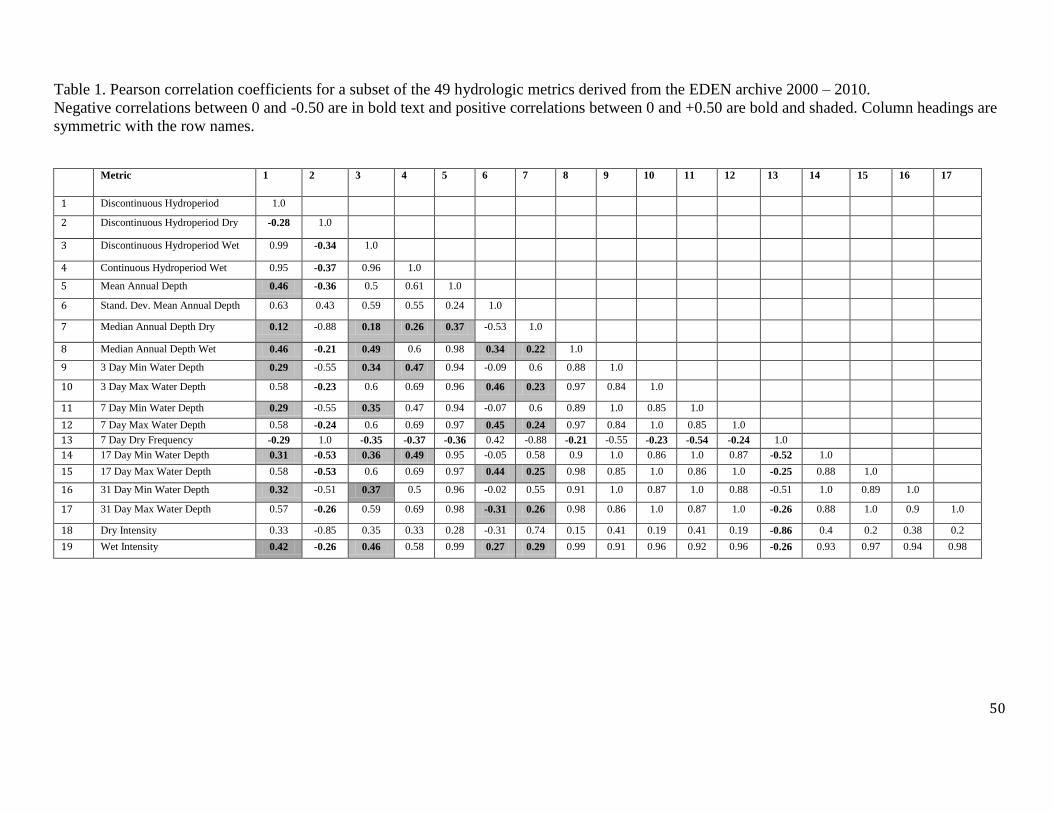
50
Table 1. Pearson correlation coefficients for a subset of the 49 hydrologic metrics derived from the EDEN archive 2000 – 2010.
Negative correlations between 0 and -0.50 are in bold text and positive correlations between 0 and +0.50 are bold and shaded. Column headings are
symmetric with the row names.
Metric 1 2 3 4 5 6 7 8 9 10 11 12 13 14 15 16 17
1 Discontinuous Hydroperiod 1.0
2 Discontinuous Hydroperiod Dry -0.28 1.0
3 Discontinuous Hydroperiod Wet 0.99 -0.34 1.0
4 Continuous Hydroperiod Wet 0.95 -0.37 0.96 1.0
5 Mean Annual Depth 0.46 -0.36 0.5 0.61 1.0
6 Stand. Dev. Mean Annual Depth 0.63 0.43 0.59 0.55 0.24 1.0
7 Median Annual Depth Dry 0.12 -0.88 0.18 0.26 0.37 -0.53 1.0
8 Median Annual Depth Wet 0.46 -0.21 0.49 0.6 0.98 0.34 0.22 1.0
9 3 Day Min Water Depth 0.29 -0.55 0.34 0.47 0.94 -0.09 0.6 0.88 1.0
10 3 Day Max Water Depth 0.58 -0.23 0.6 0.69 0.96 0.46 0.23 0.97 0.84 1.0
11 7 Day Min Water Depth 0.29 -0.55 0.35 0.47 0.94 -0.07 0.6 0.89 1.0 0.85 1.0
12 7 Day Max Water Depth 0.58 -0.24 0.6 0.69 0.97 0.45 0.24 0.97 0.84 1.0 0.85 1.0
13 7 Day Dry Frequency -0.29 1.0 -0.35 -0.37 -0.36 0.42 -0.88 -0.21 -0.55 -0.23 -0.54 -0.24 1.0
14 17 Day Min Water Depth 0.31 -0.53 0.36 0.49 0.95 -0.05 0.58 0.9 1.0 0.86 1.0 0.87 -0.52 1.0
15 17 Day Max Water Depth 0.58 -0.53 0.6 0.69 0.97 0.44 0.25 0.98 0.85 1.0 0.86 1.0 -0.25 0.88 1.0
16 31 Day Min Water Depth 0.32 -0.51 0.37 0.5 0.96 -0.02 0.55 0.91 1.0 0.87 1.0 0.88 -0.51 1.0 0.89 1.0
17 31 Day Max Water Depth 0.57 -0.26 0.59 0.69 0.98 -0.31 0.26 0.98 0.86 1.0 0.87 1.0 -0.26 0.88 1.0 0.9 1.0
18 Dry Intensity 0.33 -0.85 0.35 0.33 0.28 -0.31 0.74 0.15 0.41 0.19 0.41 0.19 -0.86 0.4 0.2 0.38 0.2
19 Wet Intensity 0.42 -0.26 0.46 0.58 0.99 0.27 0.29 0.99 0.91 0.96 0.92 0.96 -0.26 0.93 0.97 0.94 0.98
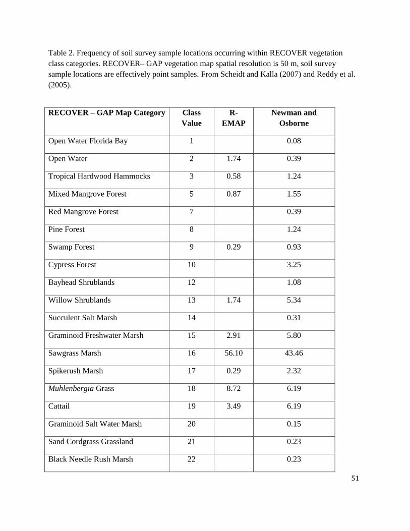
51
Table 2. Frequency of soil survey sample locations occurring within RECOVER vegetation
class categories. RECOVER– GAP vegetation map spatial resolution is 50 m, soil survey
sample locations are effectively point samples. From Scheidt and Kalla (2007) and Reddy et al.
(2005).
RECOVER – GAP Map Category Class
Value
R-
EMAP
Newman and
Osborne
Open Water Florida Bay 1 0.08
Open Water 2 1.74 0.39
Tropical Hardwood Hammocks 3 0.58 1.24
Mixed Mangrove Forest 5 0.87 1.55
Red Mangrove Forest 7 0.39
Pine Forest 8 1.24
Swamp Forest 9 0.29 0.93
Cypress Forest 10 3.25
Bayhead Shrublands 12 1.08
Willow Shrublands 13 1.74 5.34
Succulent Salt Marsh 14 0.31
Graminoid Freshwater Marsh 15 2.91 5.80
Sawgrass Marsh 16 56.10 43.46
Spikerush Marsh 17 0.29 2.32
Muhlenbergia Grass 18 8.72 6.19
Cattail 19 3.49 6.19
Graminoid Salt Water Marsh 20 0.15
Sand Cordgrass Grassland 21 0.23
Black Needle Rush Marsh 22 0.23
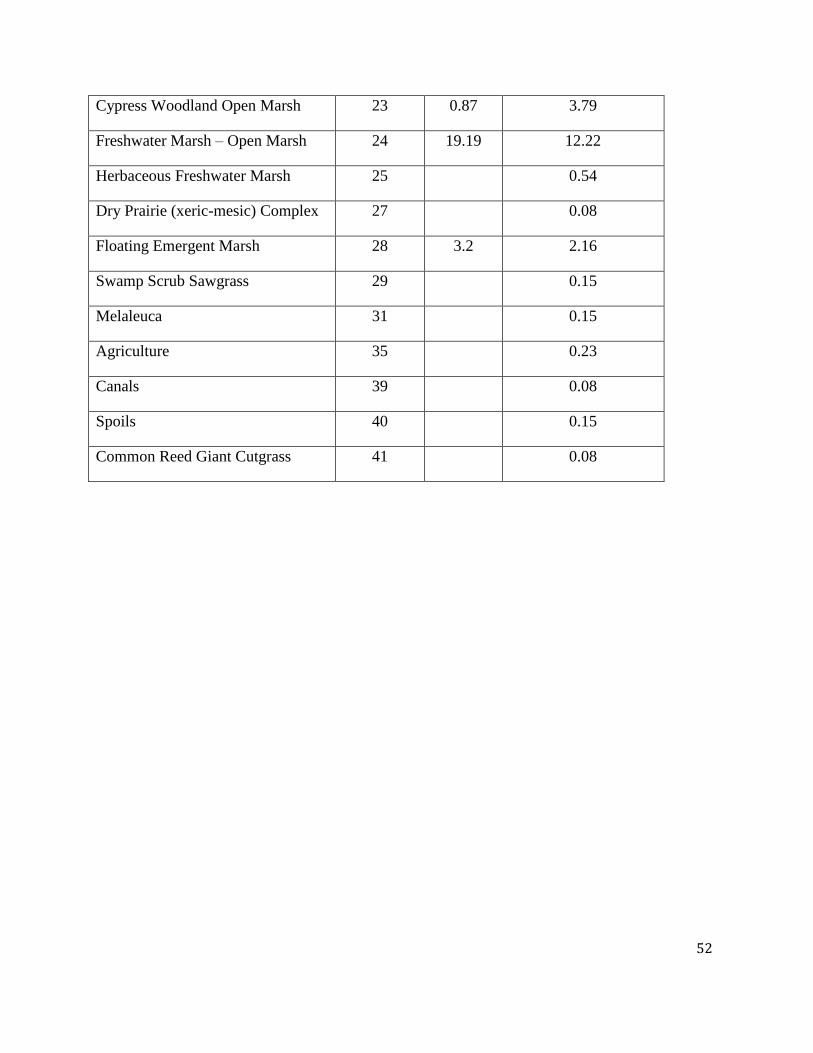
52
Cypress Woodland Open Marsh 23 0.87 3.79
Freshwater Marsh – Open Marsh 24 19.19 12.22
Herbaceous Freshwater Marsh 25 0.54
Dry Prairie (xeric-mesic) Complex 27 0.08
Floating Emergent Marsh 28 3.2 2.16
Swamp Scrub Sawgrass 29 0.15
Melaleuca 31 0.15
Agriculture 35 0.23
Canals 39 0.08
Spoils 40 0.15
Common Reed Giant Cutgrass 41 0.08
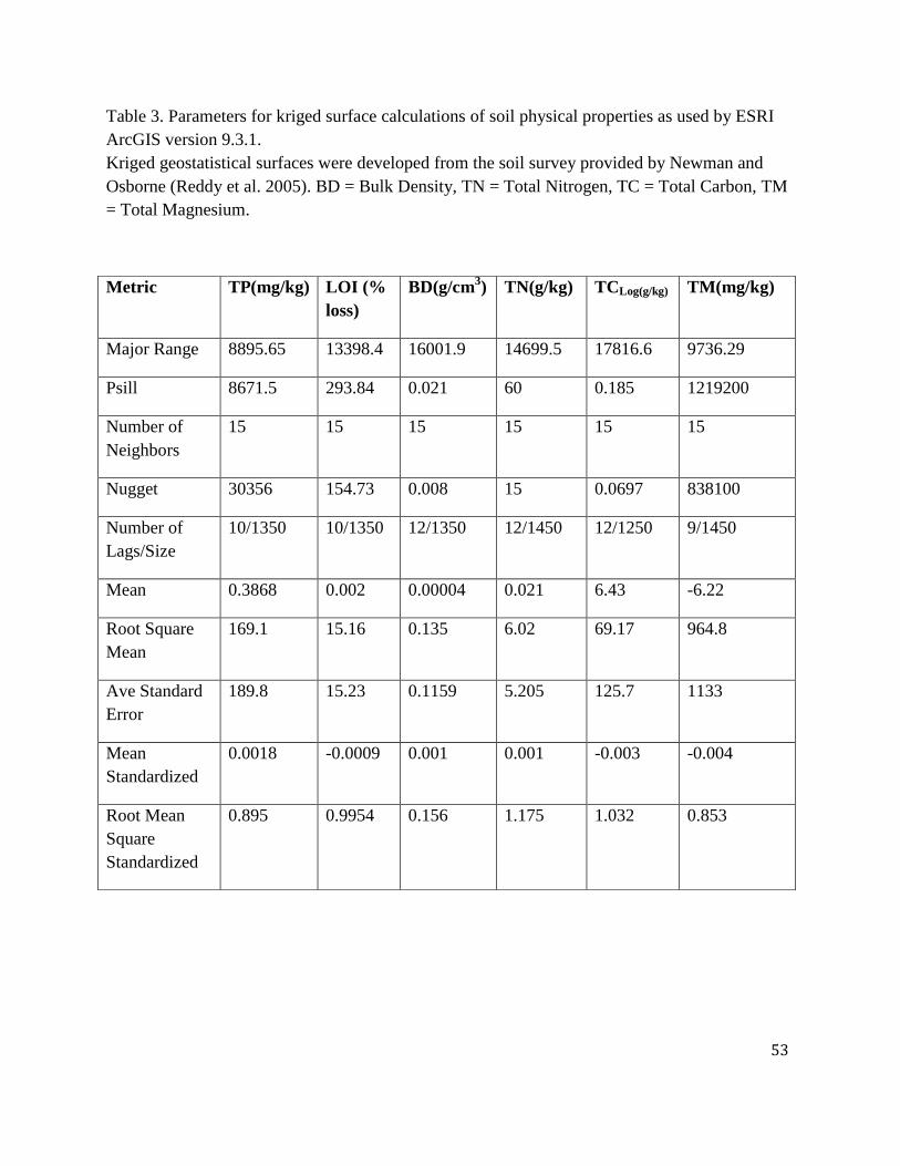
53
Table 3. Parameters for kriged surface calculations of soil physical properties as used by ESRI
ArcGIS version 9.3.1.
Kriged geostatistical surfaces were developed from the soil survey provided by Newman and
Osborne (Reddy et al. 2005). BD = Bulk Density, TN = Total Nitrogen, TC = Total Carbon, TM
= Total Magnesium.
Metric TP(mg/kg) LOI (%
loss)
BD(g/cm3) TN(g/kg) TCLog(g/kg) TM(mg/kg)
Major Range 8895.65 13398.4 16001.9 14699.5 17816.6 9736.29
Psill 8671.5 293.84 0.021 60 0.185 1219200
Number of
Neighbors
15 15 15 15 15 15
Nugget 30356 154.73 0.008 15 0.0697 838100
Number of
Lags/Size
10/1350 10/1350 12/1350 12/1450 12/1250 9/1450
Mean 0.3868 0.002 0.00004 0.021 6.43 -6.22
Root Square
Mean
169.1 15.16 0.135 6.02 69.17 964.8
Ave Standard
Error
189.8 15.23 0.1159 5.205 125.7 1133
Mean
Standardized
0.0018 -0.0009 0.001 0.001 -0.003 -0.004
Root Mean
Square
Standardized
0.895 0.9954 0.156 1.175 1.032 0.853
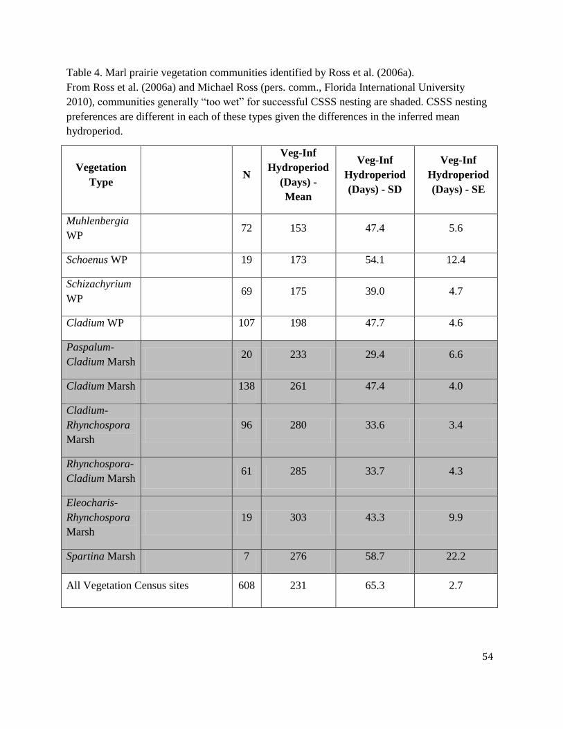
54
Table 4. Marl prairie vegetation communities identified by Ross et al. (2006a).
From Ross et al. (2006a) and Michael Ross (pers. comm., Florida International University
2010), communities generally ―too wet‖ for successful CSSS nesting are shaded. CSSS nesting
preferences are different in each of these types given the differences in the inferred mean
hydroperiod.
Vegetation
Type N
Veg-Inf
Hydroperiod
(Days) -
Mean
Veg-Inf
Hydroperiod
(Days) - SD
Veg-Inf
Hydroperiod
(Days) - SE
Muhlenbergia
WP 72 153 47.4 5.6
Schoenus WP 19 173 54.1 12.4
Schizachyrium
WP 69 175 39.0 4.7
Cladium WP 107 198 47.7 4.6
Paspalum-
Cladium Marsh 20 233 29.4 6.6
Cladium Marsh 138 261 47.4 4.0
Cladium-
Rhynchospora
Marsh
96 280 33.6 3.4
Rhynchospora-
Cladium Marsh 61 285 33.7 4.3
Eleocharis-
Rhynchospora
Marsh
19 303 43.3 9.9
Spartina Marsh 7 276 58.7 22.2
All Vegetation Census sites 608 231 65.3 2.7
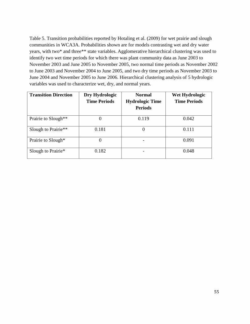
55
Table 5. Transition probabilities reported by Hotaling et al. (2009) for wet prairie and slough
communities in WCA3A. Probabilities shown are for models contrasting wet and dry water
years, with two* and three** state variables. Agglomerative hierarchical clustering was used to
identify two wet time periods for which there was plant community data as June 2003 to
November 2003 and June 2005 to November 2005, two normal time periods as November 2002
to June 2003 and November 2004 to June 2005, and two dry time periods as November 2003 to
June 2004 and November 2005 to June 2006. Hierarchical clustering analysis of 5 hydrologic
variables was used to characterize wet, dry, and normal years.
Transition Direction Dry Hydrologic
Time Periods
Normal
Hydrologic Time
Periods
Wet Hydrologic
Time Periods
Prairie to Slough** 0 0.119 0.042
Slough to Prairie** 0.181 0 0.111
Prairie to Slough* 0 - 0.091
Slough to Prairie* 0.182 - 0.048
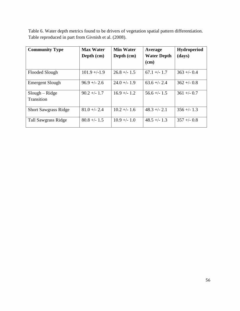
56
Table 6. Water depth metrics found to be drivers of vegetation spatial pattern differentiation.
Table reproduced in part from Givnish et al. (2008).
Community Type Max Water
Depth (cm)
Min Water
Depth (cm)
Average
Water Depth
(cm)
Hydroperiod
(days)
Flooded Slough 101.9 +/-1.9 26.8 +/- 1.5 67.1 +/- 1.7 363 +/- 0.4
Emergent Slough 96.9 +/- 2.6 24.0 +/- 1.9 63.6 +/- 2.4 362 +/- 0.8
Slough – Ridge
Transition
90.2 +/- 1.7 16.9 +/- 1.2 56.6 +/- 1.5 361 +/- 0.7
Short Sawgrass Ridge 81.0 +/- 2.4 10.2 +/- 1.6 48.3 +/- 2.1 356 +/- 1.3
Tall Sawgrass Ridge 80.8 +/- 1.5 10.9 +/- 1.0 48.5 +/- 1.3 357 +/- 0.8
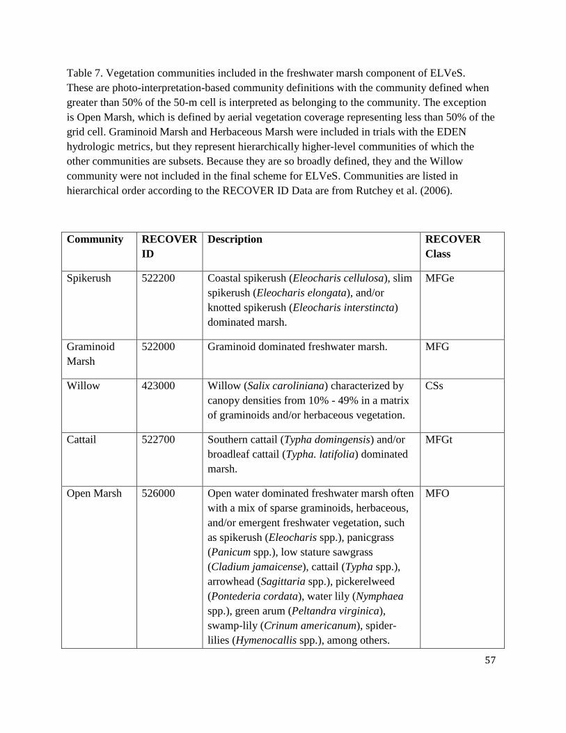
57
Table 7. Vegetation communities included in the freshwater marsh component of ELVeS.
These are photo-interpretation-based community definitions with the community defined when
greater than 50% of the 50-m cell is interpreted as belonging to the community. The exception
is Open Marsh, which is defined by aerial vegetation coverage representing less than 50% of the
grid cell. Graminoid Marsh and Herbaceous Marsh were included in trials with the EDEN
hydrologic metrics, but they represent hierarchically higher-level communities of which the
other communities are subsets. Because they are so broadly defined, they and the Willow
community were not included in the final scheme for ELVeS. Communities are listed in
hierarchical order according to the RECOVER ID Data are from Rutchey et al. (2006).
Community RECOVER
ID
Description RECOVER
Class
Spikerush 522200 Coastal spikerush (Eleocharis cellulosa), slim
spikerush (Eleocharis elongata), and/or
knotted spikerush (Eleocharis interstincta)
dominated marsh.
MFGe
Graminoid
Marsh
522000 Graminoid dominated freshwater marsh. MFG
Willow 423000 Willow (Salix caroliniana) characterized by
canopy densities from 10% - 49% in a matrix
of graminoids and/or herbaceous vegetation.
CSs
Cattail 522700 Southern cattail (Typha domingensis) and/or
broadleaf cattail (Typha. latifolia) dominated
marsh.
MFGt
Open Marsh 526000 Open water dominated freshwater marsh often
with a mix of sparse graminoids, herbaceous,
and/or emergent freshwater vegetation, such
as spikerush (Eleocharis spp.), panicgrass
(Panicum spp.), low stature sawgrass
(Cladium jamaicense), cattail (Typha spp.),
arrowhead (Sagittaria spp.), pickerelweed
(Pontederia cordata), water lily (Nymphaea
spp.), green arum (Peltandra virginica),
swamp-lily (Crinum americanum), spider-
lilies (Hymenocallis spp.), among others.
MFO
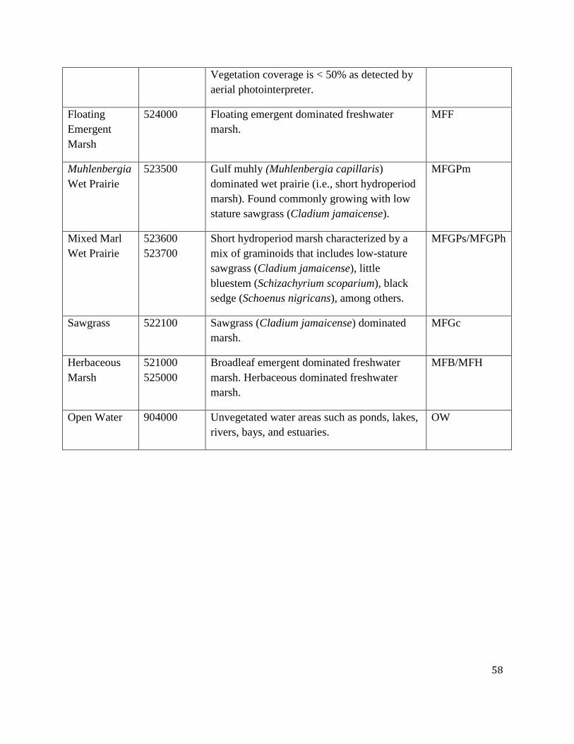
58
Vegetation coverage is < 50% as detected by
aerial photointerpreter.
Floating
Emergent
Marsh
524000 Floating emergent dominated freshwater
marsh.
MFF
Muhlenbergia
Wet Prairie
523500 Gulf muhly (Muhlenbergia capillaris)
dominated wet prairie (i.e., short hydroperiod
marsh). Found commonly growing with low
stature sawgrass (Cladium jamaicense).
MFGPm
Mixed Marl
Wet Prairie
523600
523700
Short hydroperiod marsh characterized by a
mix of graminoids that includes low-stature
sawgrass (Cladium jamaicense), little
bluestem (Schizachyrium scoparium), black
sedge (Schoenus nigricans), among others.
MFGPs/MFGPh
Sawgrass 522100 Sawgrass (Cladium jamaicense) dominated
marsh.
MFGc
Herbaceous
Marsh
521000
525000
Broadleaf emergent dominated freshwater
marsh. Herbaceous dominated freshwater
marsh.
MFB/MFH
Open Water 904000 Unvegetated water areas such as ponds, lakes,
rivers, bays, and estuaries.
OW
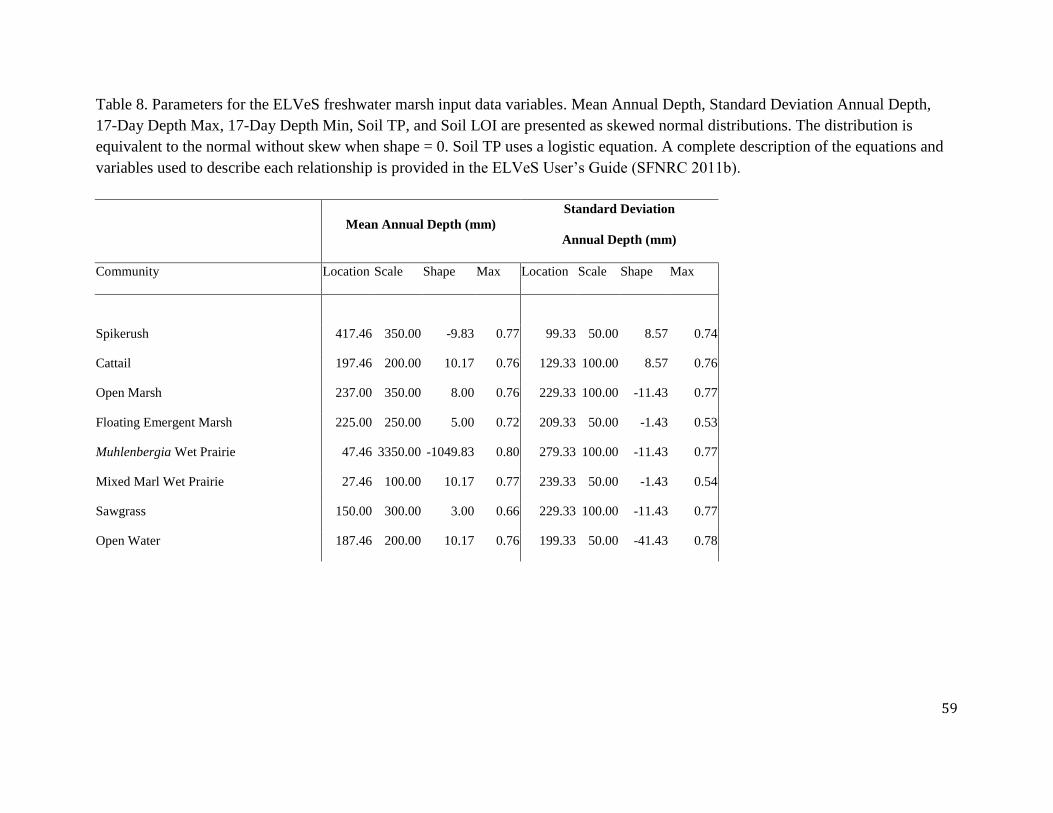
59
Table 8. Parameters for the ELVeS freshwater marsh input data variables. Mean Annual Depth, Standard Deviation Annual Depth,
17-Day Depth Max, 17-Day Depth Min, Soil TP, and Soil LOI are presented as skewed normal distributions. The distribution is
equivalent to the normal without skew when shape = 0. Soil TP uses a logistic equation. A complete description of the equations and
variables used to describe each relationship is provided in the ELVeS User’s Guide (SFNRC 2011b).
Mean Annual Depth (mm)
Standard Deviation
Annual Depth (mm)
Community Location Scale Shape Max Location Scale Shape Max
Spikerush 417.46 350.00 -9.83 0.77 99.33 50.00 8.57 0.74
Cattail 197.46 200.00 10.17 0.76 129.33 100.00 8.57 0.76
Open Marsh 237.00 350.00 8.00 0.76 229.33 100.00 -11.43 0.77
Floating Emergent Marsh 225.00 250.00 5.00 0.72 209.33 50.00 -1.43 0.53
Muhlenbergia Wet Prairie 47.46 3350.00 -1049.83 0.80 279.33 100.00 -11.43 0.77
Mixed Marl Wet Prairie 27.46 100.00 10.17 0.77 239.33 50.00 -1.43 0.54
Sawgrass 150.00 300.00 3.00 0.66 229.33 100.00 -11.43 0.77
Open Water 187.46 200.00 10.17 0.76 199.33 50.00 -41.43 0.78
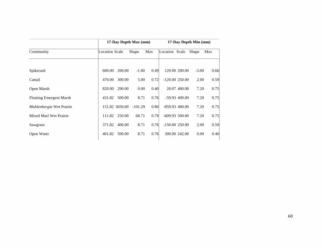
60
17-Day Depth Max (mm) 17-Day Depth Min (mm)
Community Location Scale Shape Max Location Scale Shape Max
Spikerush 600.00 200.00 -1.00 0.49 120.00 200.00 -3.00 0.66
Cattail 470.00 300.00 5.00 0.72 -120.00 250.00 2.00 0.59
Open Marsh 820.00 290.00 0.00 0.40 20.07 400.00 7.20 0.75
Floating Emergent Marsh 431.82 500.00 8.71 0.76 -59.93 400.00 7.20 0.75
Muhlenbergia Wet Prairie 151.82 3650.00 -101.29 0.80 -859.93 400.00 7.20 0.75
Mixed Marl Wet Prairie 111.82 250.00 68.71 0.79 -609.93 500.00 7.20 0.75
Sawgrass 371.82 400.00 8.71 0.76 -150.00 250.00 2.00 0.59
Open Water 401.82 500.00 8.71 0.76 300.00 242.00 0.00 0.40
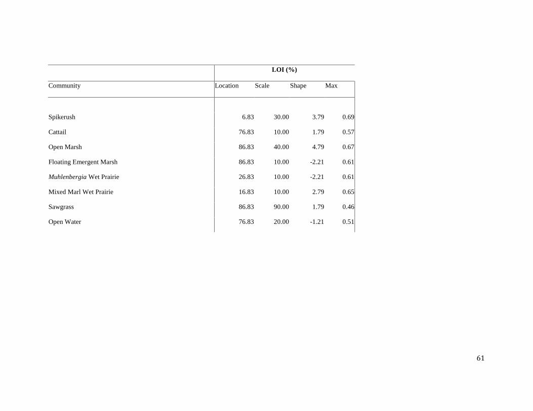
61
LOI (%)
Community Location Scale Shape Max
Spikerush 6.83 30.00 3.79 0.69
Cattail 76.83 10.00 1.79 0.57
Open Marsh 86.83 40.00 4.79 0.67
Floating Emergent Marsh 86.83 10.00 -2.21 0.61
Muhlenbergia Wet Prairie 26.83 10.00 -2.21 0.61
Mixed Marl Wet Prairie 16.83 10.00 2.79 0.65
Sawgrass 86.83 90.00 1.79 0.46
Open Water 76.83 20.00 -1.21 0.51

62
TP (mg/kg)
Community Mean1 Mean2 Gradient
Spikerush 350.00 460.00 -1
Cattail 500.00 650.00 1
Open Marsh 360.00 475.00 -1
Floating Emergent Marsh 390.00 450.00 -1
Muhlenbergia Wet Prairie 180.00 380.00 -1
Mixed Marl Wet Prairie 260.00 475.00 -1
Sawgrass 350.00 500.00 -1
Open Water 320.00 460.00 -1
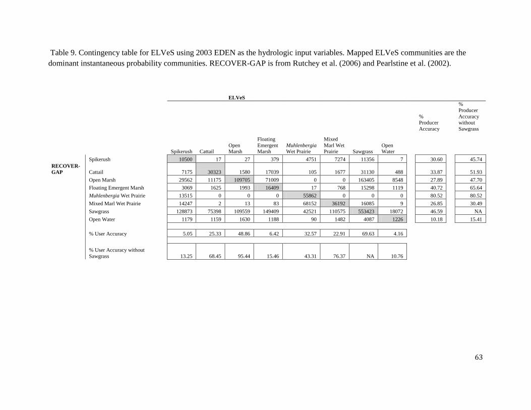
63
Table 9. Contingency table for ELVeS using 2003 EDEN as the hydrologic input variables. Mapped ELVeS communities are the
dominant instantaneous probability communities. RECOVER-GAP is from Rutchey et al. (2006) and Pearlstine et al. (2002).
ELVeS
% Producer
Accuracy
%
Producer
Accuracy without
Sawgrass
Spikerush Cattail Open Marsh
Floating
Emergent Marsh
Muhlenbergia Wet Prairie
Mixed
Marl Wet Prairie Sawgrass
Open Water
Spikerush 10500 17 27 379 4751 7274 11356 7 30.60 45.74
RECOVER-
GAP Cattail 7175 30323 1580 17039 105 1677 31130 488 33.87 51.93
Open Marsh 29562 11175 109705 71009 0 0 163405 8548 27.89 47.70
Floating Emergent Marsh 3069 1625 1993 16409 17 768 15298 1119 40.72 65.64
Muhlenbergia Wet Prairie 13515 0 0 0 55862 0 0 0 80.52 80.52
Mixed Marl Wet Prairie 14247 2 13 83 68152 36192 16085 9 26.85 30.49
Sawgrass 128873 75398 109559 149409 42521 110575 553423 18072 46.59 NA
Open Water 1179 1159 1630 1188 90 1482 4087 1226 10.18 15.41
% User Accuracy 5.05 25.33 48.86 6.42 32.57 22.91 69.63 4.16
% User Accuracy without
Sawgrass 13.25 68.45 95.44 15.46 43.31 76.37 NA 10.76
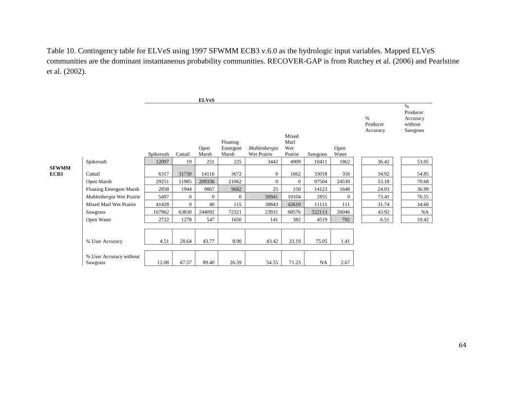
64
Table 10. Contingency table for ELVeS using 1997 SFWMM ECB3 v.6.0 as the hydrologic input variables. Mapped ELVeS
communities are the dominant instantaneous probability communities. RECOVER-GAP is from Rutchey et al. (2006) and Pearlstine
et al. (2002).
ELVeS
%
Producer
Accuracy
%
Producer
Accuracy
without
Sawgrass
Spikerush Cattail
Open
Marsh
Floating
Emergent
Marsh
Muhlenbergia
Wet Prairie
Mixed Marl
Wet
Prairie Sawgrass
Open
Water
Spikerush 12097 19 251 225 3442 4909 10411 1862 36.42 53.05
SFWMM
ECB3 Cattail 6317 31730 14116 3672 0 1662 33018 356 34.92 54.85
Open Marsh 29251 11985 209336 21062 0 0 97504 24530 53.18 70.68
Floating Emergent Marsh 2858 1944 9867 9682 25 150 14123 1648 24.03 36.99
Muhlenbergia Wet Prairie 5497 0 0 0 50941 10104 2855 0 73.41 76.55
Mixed Marl Wet Prairie 41428 0 40 115 38843 42610 11115 111 31.74 34.60
Sawgrass 167962 63830 244092 72321 23931 68576 522113 26046 43.92 NA
Open Water 2722 1278 547 1650 141 382 4519 782 6.51 10.42
% User Accuracy 4.51 28.64 43.77 8.90 43.42 33.19 75.05 1.41
% User Accuracy without
Sawgrass 12.08 67.57 89.40 26.59 54.55 71.23 NA 2.67
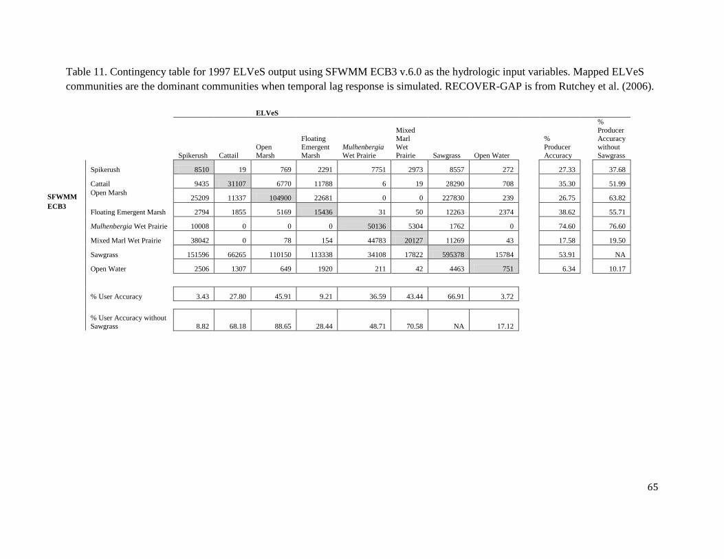
65
Table 11. Contingency table for 1997 ELVeS output using SFWMM ECB3 v.6.0 as the hydrologic input variables. Mapped ELVeS
communities are the dominant communities when temporal lag response is simulated. RECOVER-GAP is from Rutchey et al. (2006).
ELVeS
Spikerush Cattail
Open
Marsh
Floating
Emergent
Marsh
Mulhenbergia
Wet Prairie
Mixed Marl
Wet
Prairie Sawgrass Open Water
%
Producer
Accuracy
%
Producer Accuracy
without
Sawgrass
Spikerush 8510 19 769 2291 7751 2973 8557 272
27.33
37.68
Cattail 9435 31107 6770 11788 6 19 28290 708
35.30
51.99
Open Marsh 25209 11337 104900 22681 0 0 227830 239
26.75
63.82
Floating Emergent Marsh 2794 1855 5169 15436 31 50 12263 2374
38.62
55.71
Mulhenbergia Wet Prairie 10008 0 0 0 50136 5304 1762 0
74.60
76.60
Mixed Marl Wet Prairie 38042 0 78 154 44783 20127 11269 43
17.58
19.50
Sawgrass 151596 66265 110150 113338 34108 17822 595378 15784
53.91
NA
Open Water 2506 1307 649 1920 211 42 4463 751
6.34
10.17
% User Accuracy 3.43 27.80 45.91 9.21 36.59 43.44 66.91 3.72
% User Accuracy without
Sawgrass 8.82 68.18 88.65 28.44 48.71 70.58 NA 17.12
SFWMM
ECB3
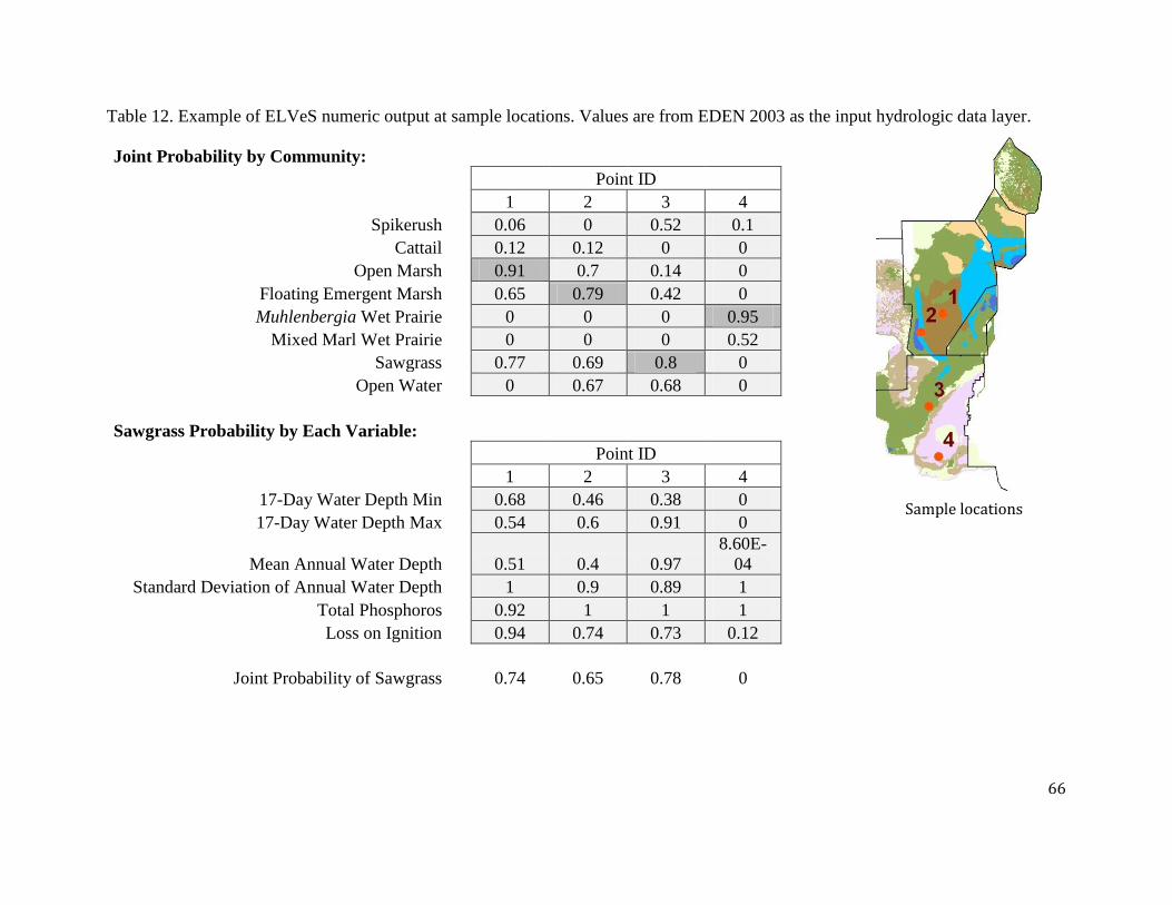
66
Table 12. Example of ELVeS numeric output at sample locations. Values are from EDEN 2003 as the input hydrologic data layer.
Joint Probability by Community:
Point ID
1 2 3 4
Spikerush 0.06 0 0.52 0.1
Cattail 0.12 0.12 0 0
Open Marsh 0.91 0.7 0.14 0
Floating Emergent Marsh 0.65 0.79 0.42 0
Muhlenbergia Wet Prairie 0 0 0 0.95
Mixed Marl Wet Prairie 0 0 0 0.52
Sawgrass 0.77 0.69 0.8 0
Open Water 0 0.67 0.68 0
Sawgrass Probability by Each Variable:
Point ID
1 2 3 4
17-Day Water Depth Min
0.68 0.46 0.38 0
17-Day Water Depth Max
0.54 0.6 0.91 0
Mean Annual Water Depth
0.51 0.4 0.97
8.60E-
04
Standard Deviation of Annual Water Depth
1 0.9 0.89 1
Total Phosphoros
0.92 1 1 1
Loss on Ignition
0.94 0.74 0.73 0.12
Joint Probability of Sawgrass
0.74 0.65 0.78 0
Sample locations
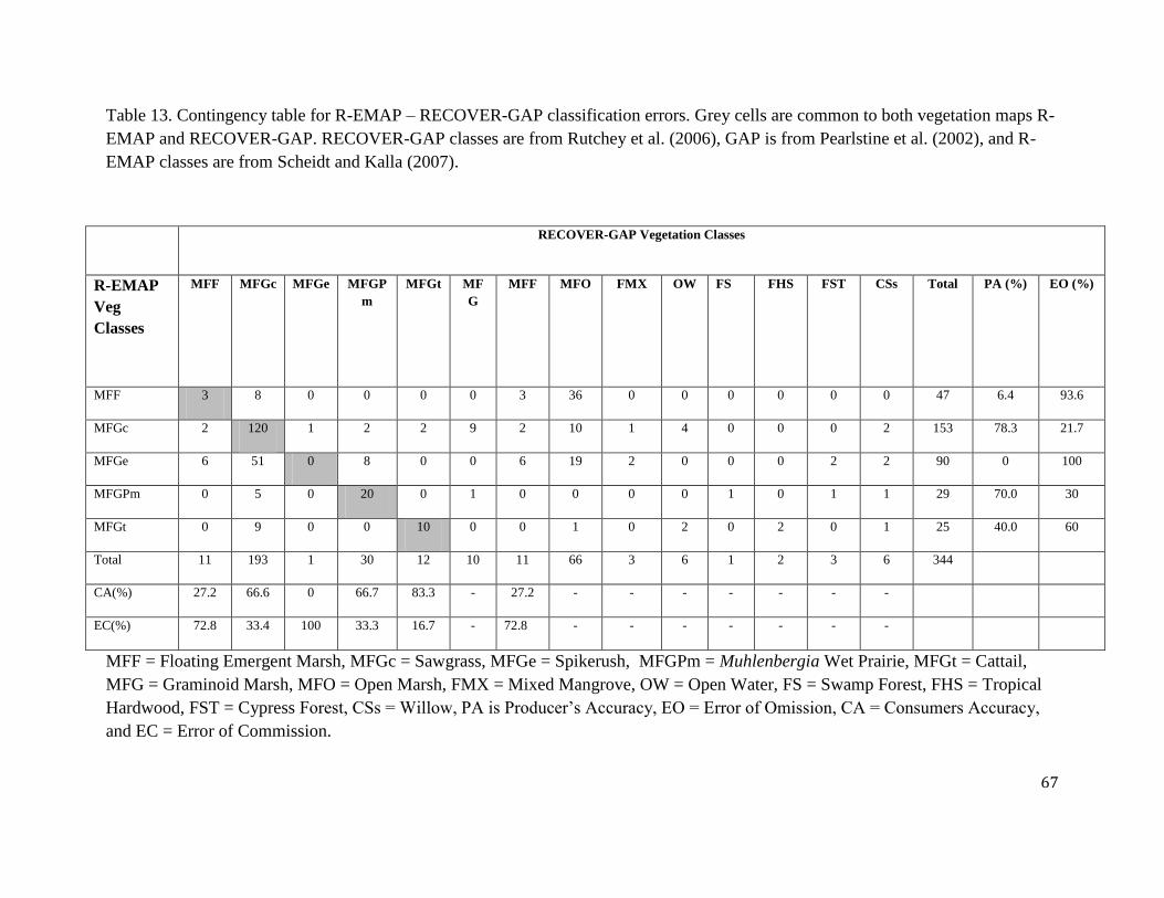
67
Table 13. Contingency table for R-EMAP – RECOVER-GAP classification errors. Grey cells are common to both vegetation maps R-
EMAP and RECOVER-GAP. RECOVER-GAP classes are from Rutchey et al. (2006), GAP is from Pearlstine et al. (2002), and R-
EMAP classes are from Scheidt and Kalla (2007).
RECOVER-GAP Vegetation Classes
R-EMAP
Veg
Classes
MFF MFGc MFGe MFGP
m
MFGt MF
G
MFF MFO FMX OW FS FHS FST CSs Total PA (%) EO (%)
MFF 3 8 0 0 0 0 3 36 0 0 0 0 0 0 47 6.4 93.6
MFGc 2 120 1 2 2 9 2 10 1 4 0 0 0 2 153 78.3 21.7
MFGe 6 51 0 8 0 0 6 19 2 0 0 0 2 2 90 0 100
MFGPm 0 5 0 20 0 1 0 0 0 0 1 0 1 1 29 70.0 30
MFGt 0 9 0 0 10 0 0 1 0 2 0 2 0 1 25 40.0 60
Total 11 193 1 30 12 10 11 66 3 6 1 2 3 6 344
CA(%) 27.2 66.6 0 66.7 83.3 - 27.2 - - - - - - -
EC(%) 72.8 33.4 100 33.3 16.7 - 72.8 - - - - - - -
MFF = Floating Emergent Marsh, MFGc = Sawgrass, MFGe = Spikerush, MFGPm = Muhlenbergia Wet Prairie, MFGt = Cattail,
MFG = Graminoid Marsh, MFO = Open Marsh, FMX = Mixed Mangrove, OW = Open Water, FS = Swamp Forest, FHS = Tropical
Hardwood, FST = Cypress Forest, CSs = Willow, PA is Producer’s Accuracy, EO = Error of Omission, CA = Consumers Accuracy,
and EC = Error of Commission.
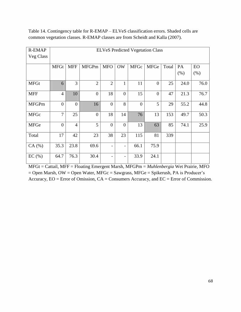
68
Table 14. Contingency table for R-EMAP – ELVeS classification errors. Shaded cells are
common vegetation classes. R-EMAP classes are from Scheidt and Kalla (2007).
R-EMAP
Veg Class
ELVeS Predicted Vegetation Class
MFGt MFF MFGPm MFO OW MFGc MFGe Total PA
(%)
EO
(%)
MFGt 6 3 2 2 1 11 0 25 24.0 76.0
MFF 4 10 0 18 0 15 0 47 21.3 76.7
MFGPm 0 0 16 0 8 0 5 29 55.2 44.8
MFGc 7 25 0 18 14 76 13 153 49.7 50.3
MFGe 0 4 5 0 0 13 63 85 74.1 25.9
Total 17 42 23 38 23 115 81 339
CA (%) 35.3 23.8 69.6 - - 66.1 75.9
EC (%) 64.7 76.3 30.4 - - 33.9 24.1
MFGt = Cattail, MFF = Floating Emergent Marsh, MFGPm = Muhlenbergia Wet Prairie, MFO
= Open Marsh, OW = Open Water, MFGc = Sawgrass, MFGe = Spikerush, PA is Producer’s
Accuracy, EO = Error of Omission, CA = Consumers Accuracy, and EC = Error of Commission.

69
LIST OF FIGURES
Figure 1. Combined vegetation classification of the ELVeS Everglades spatial domain. ............................... 71
Figure 2. RECOVER-GAP classification showing the 8 classes simulated within the ELVeS freshwater
marsh and wet prairie model (Pearlstine et al. 2002, Rutchey et al. 2006). No color indicates other
vegetation types not modeled in this version of ELVeS. ............................................................................................ 72
Figure 3. Schematic diagram of the ELVeS model. ..................................................................................................... 73
Figure 4. Site location map of R-EMAP (red triangles) and Newman and Osborne (black stars) soil
surveys. (Reddy et al. 2005, Scheidt and Kalla 2007). ................................................................................................ 74
Figure 5. Non-linear response patterns to P concentrations (Figure from Hagerthey et al. 2008, used with
permission of the Ecological Society of America). ...................................................................................................... 75
Figure 6. Transition trajectories that occur when the system moves from an oligotrophic to a more
eutrophic state (Figure from Hagerthey et al. 2008, used with permission of the Ecological Society of
America)..................................................................................................................................................................................... 76
Figure 7. Transition rate in multi-state wetlands succession (Figure from Zweig and Kitchens 2009, used
with permission of the Ecological Society of America). ............................................................................................ 77
Figure 8. Hydrographs at two ENP sites, NE2 and NP203 (top), and two WCA3A sites, Site64 and 3AS.
2003 is highlighted to illustrate its selection as a normal year for stage heights (Figure from U.S.
Geological Survey 2010a). ................................................................................................................................................... 78
Figure 9. 2003 input data layers. Hydrologic layers are derived from EDEN (U.S. Geological Survey
2010b). Soil TP and Soil LOI layers are derived from Newman and Osborne (Reddy et al. 2005). ............ 79
Figure 10. Skewed normal distributions for each of the community types for five of the variables used in
the freshwater marsh component of ELVeS. This figure illustrates the extent of overlap among
communities and the separation of different communities by different hydrologic variables. See Appendix
C for additional details. ......................................................................................................................................................... 80
Figure 11. Logistic equation distributions for vegetation community response to soil TP. ............................ 81
Figure 12. Schematic diagram of the approach used to introduce temporal lags into ELVeS community
transitions. .................................................................................................................................................................................. 82
Figure 13. Instantaneous joint probabilities for sawgrass (used as an example community) are the product
of the conditional probabilities for each of the variables. Probabilites were derived from EDEN 2003
input hydrology and Newman and Osborne (Reddy et al. 2005) survey data. .................................................... 83
Figure 14. Joint instantaneous probabilities for each of the vegetation communities using EDEN 2003
input hydrology and Newman and Osborne (Reddy et al. 2005) soil survey data. ............................................ 84

70
Figure 15. RECOVER-GAP classification of fresh water marsh communities at 50 m spatial resolution
(left). ELVeS instantaneous probability dominant vegetation (middle) and instantaneous probability
secondary vegetation (right), both at 400 m resolution. ELVeS results are from EDEN 2003 input
hydrology. .................................................................................................................................................................................. 85
Figure 16. RECOVER-GAP classification of freshwater marsh communities at 50 m spatial resolution
(left). ELVeS instantaneous probability dominant vegetation from EDEN 2003 hydrology (middle) at 400
m resolution and ELVeS instantaneous probability dominant vegetation from SFWMM ECB3 1997
hydrology (right) at 500 m resolution. .............................................................................................................................. 86
Figure 17. Gage height at 3 locations in 1997 (blue) and 2003 (red). Right: Distribution of water depths
from EDEN and SFWMM ECB3 for the same years. ................................................................................................. 87
Figure 18. RECOVER-GAP classification of freshwater marsh communities at 50 m spatial resolution
(left). ELVeS instantaneous probability dominant communities from SFWMM ECB3 1997 hydrology
(middle) and dominant communities when temporal lags are included in the model (right). ......................... 88
Figure 19. Illustration of accuracy assessment measures. .......................................................................................... 89
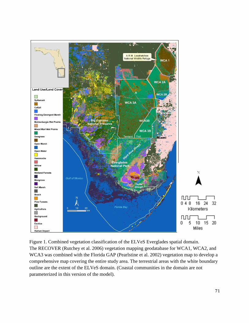
71
Figure 1. Combined vegetation classification of the ELVeS Everglades spatial domain.
The RECOVER (Rutchey et al. 2006) vegetation mapping geodatabase for WCA1, WCA2, and
WCA3 was combined with the Florida GAP (Pearlstine et al. 2002) vegetation map to develop a
comprehensive map covering the entire study area. The terrestrial areas with the white boundary
outline are the extent of the ELVeS domain. (Coastal communities in the domain are not
parameterized in this version of the model).
A
WCA3B
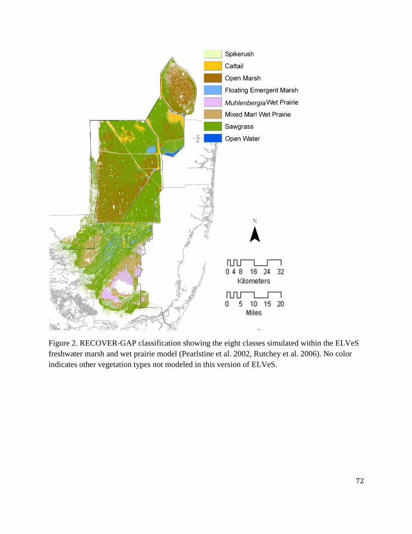
72
Figure 2. RECOVER-GAP classification showing the eight classes simulated within the ELVeS
freshwater marsh and wet prairie model (Pearlstine et al. 2002, Rutchey et al. 2006). No color
indicates other vegetation types not modeled in this version of ELVeS.
Muhlenbergia
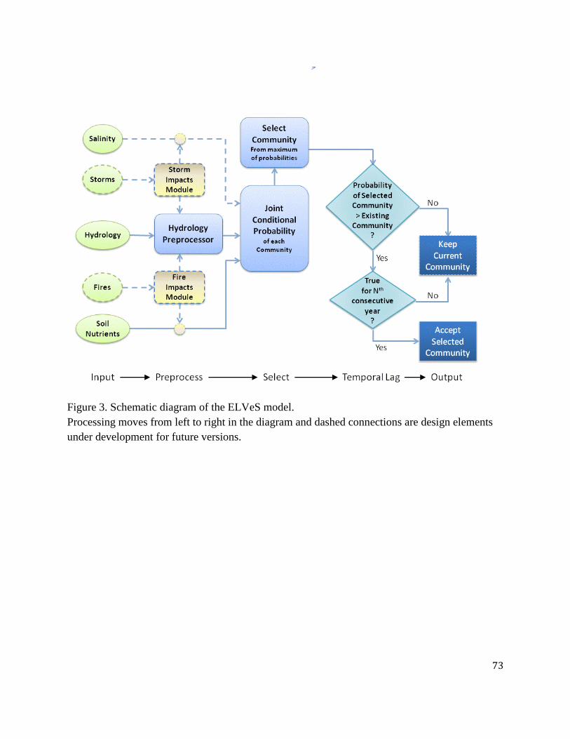
73
Figure 3. Schematic diagram of the ELVeS model.
Processing moves from left to right in the diagram and dashed connections are design elements
under development for future versions.
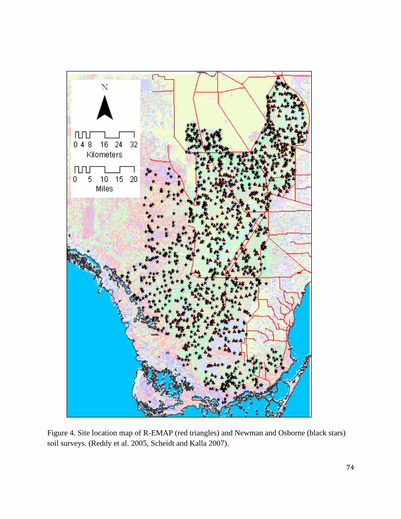
74
Figure 4. Site location map of R-EMAP (red triangles) and Newman and Osborne (black stars)
soil surveys. (Reddy et al. 2005, Scheidt and Kalla 2007).
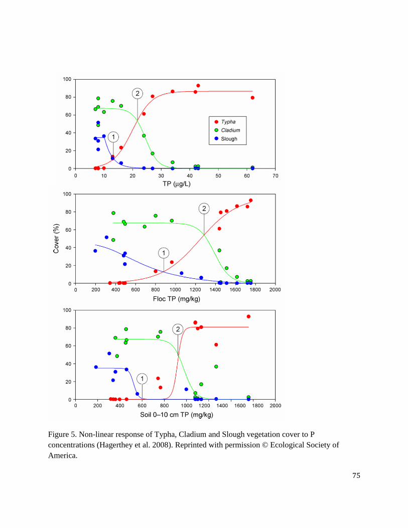
75
Figure 5. Non-linear response of Typha, Cladium and Slough vegetation cover to P
concentrations (Hagerthey et al. 2008). Reprinted with permission © Ecological Society of
America.
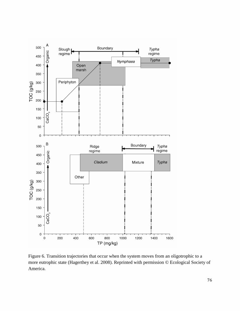
76
Figure 6. Transition trajectories that occur when the system moves from an oligotrophic to a
more eutrophic state (Hagerthey et al. 2008). Reprinted with permission © Ecological Society of
America.
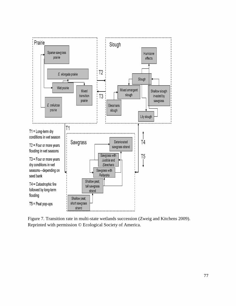
77
Figure 7. Transition rate in multi-state wetlands succession (Zweig and Kitchens 2009).
Reprinted with permission © Ecological Society of America.
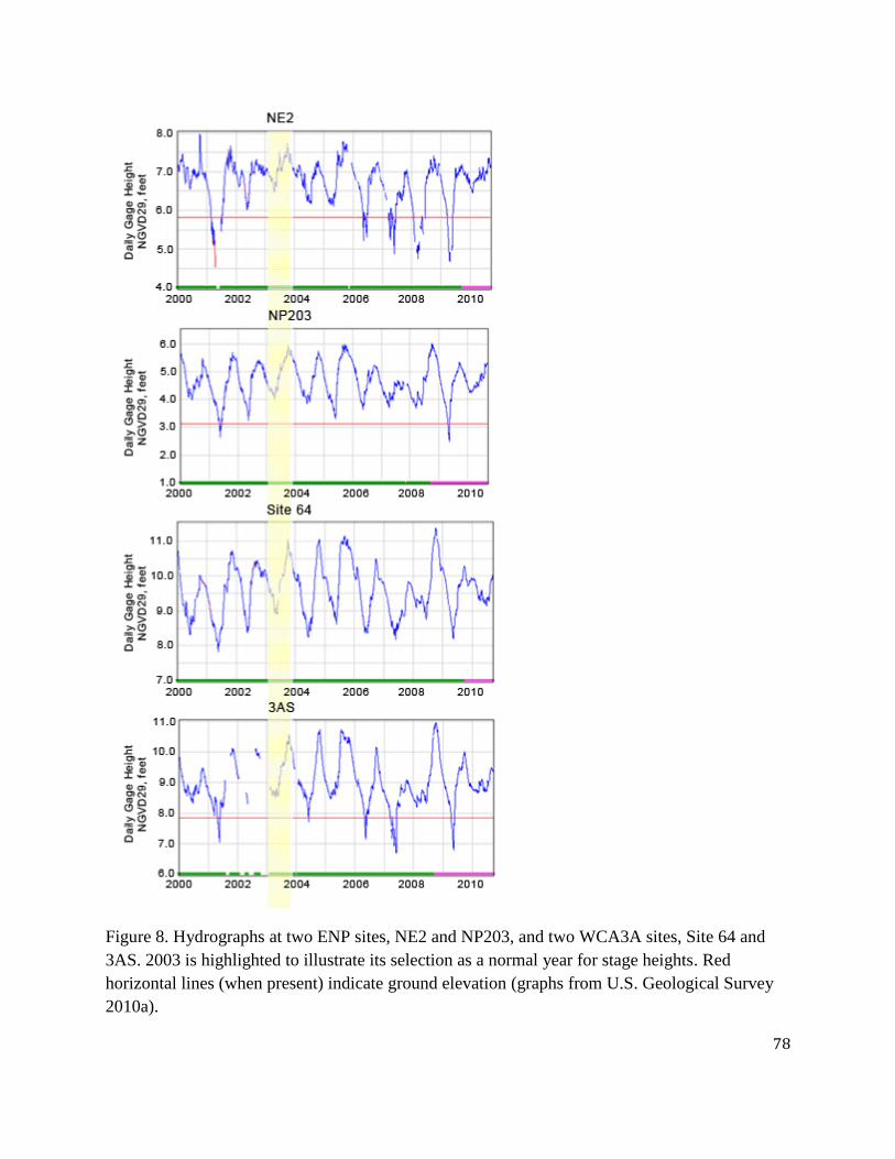
78
Figure 8. Hydrographs at two ENP sites, NE2 and NP203, and two WCA3A sites, Site 64 and
3AS. 2003 is highlighted to illustrate its selection as a normal year for stage heights. Red
horizontal lines (when present) indicate ground elevation (graphs from U.S. Geological Survey
2010a).
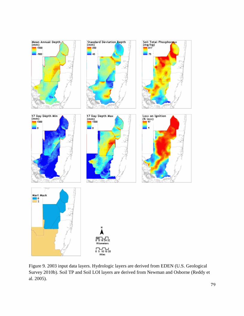
79
Figure 9. 2003 input data layers. Hydrologic layers are derived from EDEN (U.S. Geological
Survey 2010b). Soil TP and Soil LOI layers are derived from Newman and Osborne (Reddy et
al. 2005).
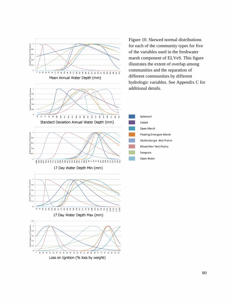
80
Figure 10. Skewed normal distributions
for each of the community types for five
of the variables used in the freshwater
marsh component of ELVeS. This figure
illustrates the extent of overlap among
communities and the separation of
different communities by different
hydrologic variables. See Appendix C for
additional details.
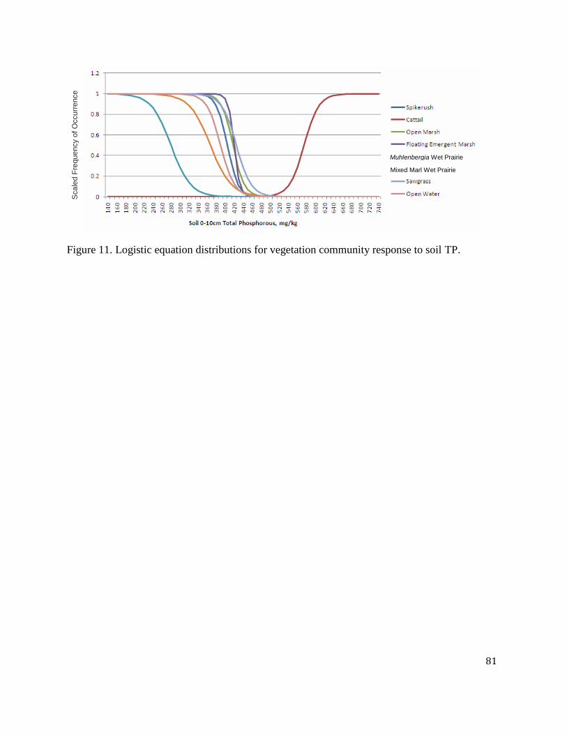
81
Figure 11. Logistic equation distributions for vegetation community response to soil TP.
Sca
led F
requ
en
cy o
f O
ccu
rre
nce
Muhlenbergia Wet Prairie
Mixed Marl Wet Prairie
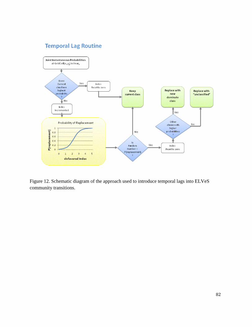
82
Figure 12. Schematic diagram of the approach used to introduce temporal lags into ELVeS
community transitions.
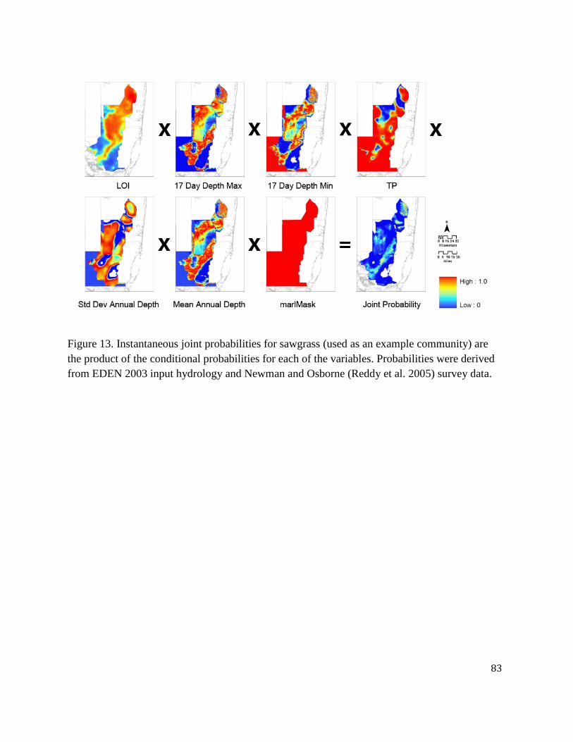
83
Figure 13. Instantaneous joint probabilities for sawgrass (used as an example community) are
the product of the conditional probabilities for each of the variables. Probabilities were derived
from EDEN 2003 input hydrology and Newman and Osborne (Reddy et al. 2005) survey data.
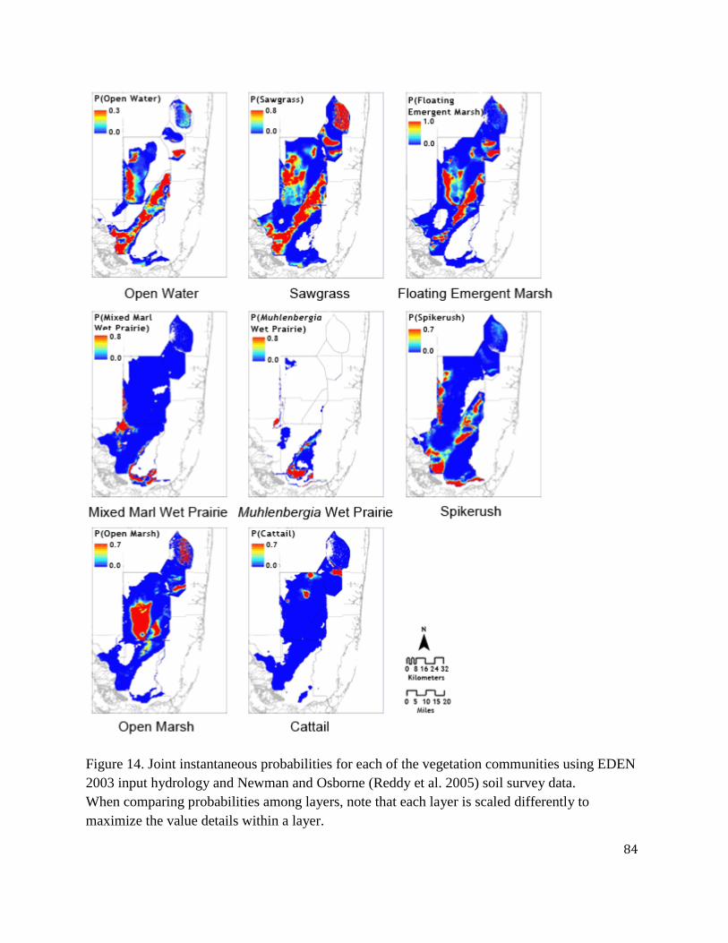
84
Figure 14. Joint instantaneous probabilities for each of the vegetation communities using EDEN
2003 input hydrology and Newman and Osborne (Reddy et al. 2005) soil survey data.
When comparing probabilities among layers, note that each layer is scaled differently to
maximize the value details within a layer.
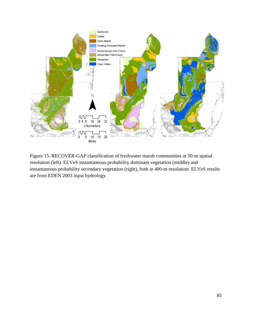
85
Figure 15. RECOVER-GAP classification of freshwater marsh communities at 50-m spatial
resolution (left). ELVeS instantaneous probability dominant vegetation (middle) and
instantaneous probability secondary vegetation (right), both at 400-m resolution. ELVeS results
are from EDEN 2003 input hydrology.
Muhlenbergia Wet Prairie
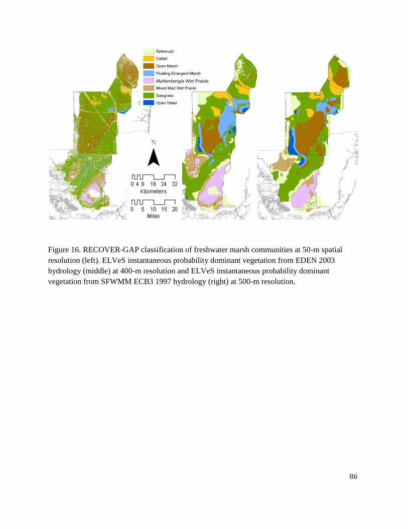
86
Figure 16. RECOVER-GAP classification of freshwater marsh communities at 50-m spatial
resolution (left). ELVeS instantaneous probability dominant vegetation from EDEN 2003
hydrology (middle) at 400-m resolution and ELVeS instantaneous probability dominant
vegetation from SFWMM ECB3 1997 hydrology (right) at 500-m resolution.
Muhlenbergia Wet Prairie
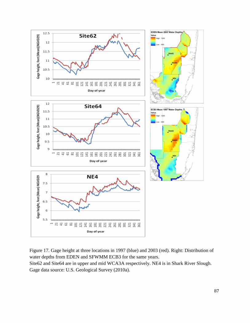
87
Figure 17. Gage height at three locations in 1997 (blue) and 2003 (red). Right: Distribution of
water depths from EDEN and SFWMM ECB3 for the same years.
Site62 and Site64 are in upper and mid WCA3A respectively. NE4 is in Shark River Slough.
Gage data source: U.S. Geological Survey (2010a).
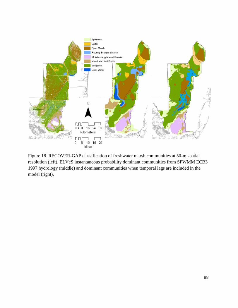
88
Figure 18. RECOVER-GAP classification of freshwater marsh communities at 50-m spatial
resolution (left). ELVeS instantaneous probability dominant communities from SFWMM ECB3
1997 hydrology (middle) and dominant communities when temporal lags are included in the
model (right).
Muhlenbergia Wet Prairie
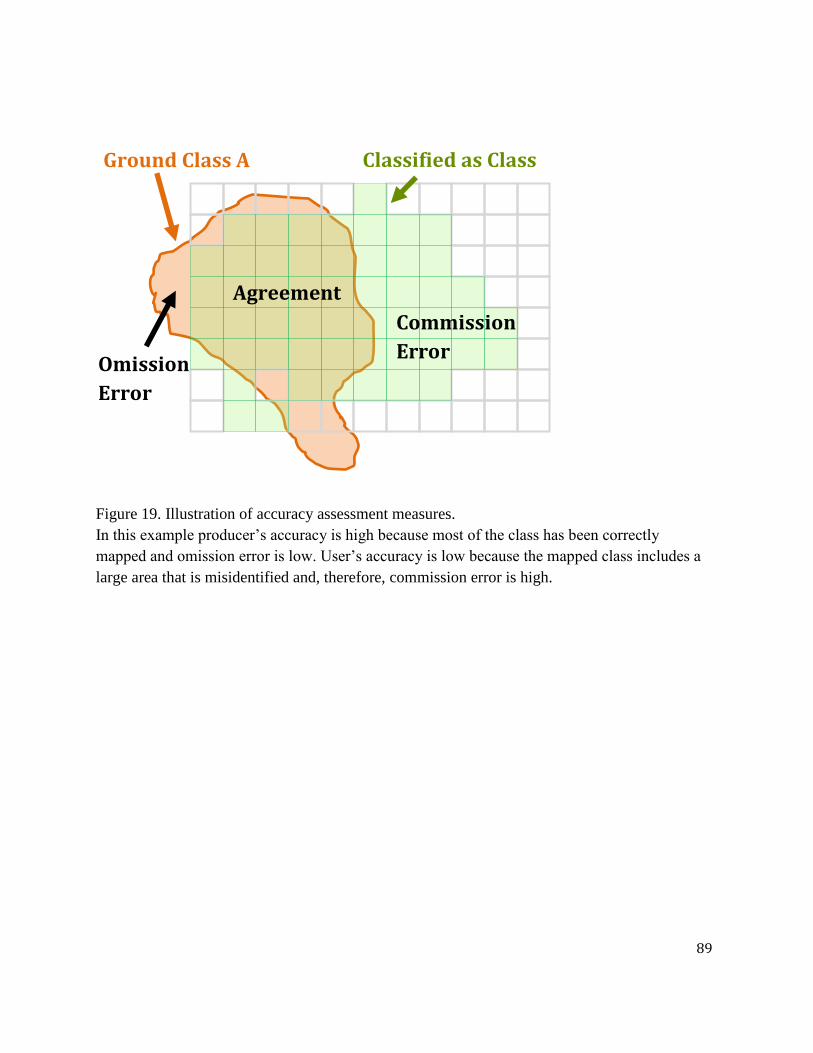
89
Figure 19. Illustration of accuracy assessment measures.
In this example producer’s accuracy is high because most of the class has been correctly
mapped and omission error is low. User’s accuracy is low because the mapped class includes a
large area that is misidentified and, therefore, commission error is high.
Ground Class A
Omission
Error
Classified as Class
A
Agreement
Commission
Error
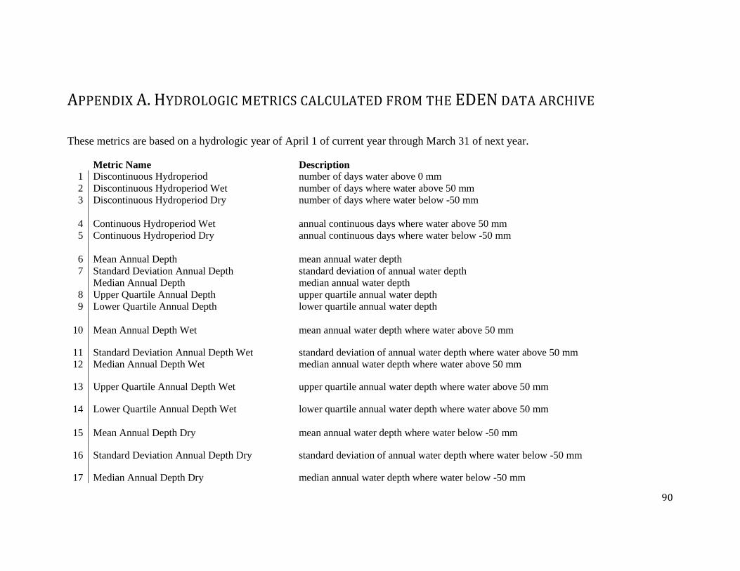
90
APPENDIX A. HYDROLOGIC METRICS CALCULATED FROM THE EDEN DATA ARCHIVE
These metrics are based on a hydrologic year of April 1 of current year through March 31 of next year.
Metric Name Description
1 Discontinuous Hydroperiod number of days water above 0 mm
2 Discontinuous Hydroperiod Wet number of days where water above 50 mm
3 Discontinuous Hydroperiod Dry number of days where water below -50 mm
4 Continuous Hydroperiod Wet annual continuous days where water above 50 mm
5 Continuous Hydroperiod Dry annual continuous days where water below -50 mm
6 Mean Annual Depth mean annual water depth
7 Standard Deviation Annual Depth standard deviation of annual water depth
Median Annual Depth median annual water depth
8 Upper Quartile Annual Depth upper quartile annual water depth
9 Lower Quartile Annual Depth lower quartile annual water depth
10 Mean Annual Depth Wet mean annual water depth where water above 50 mm
11 Standard Deviation Annual Depth Wet standard deviation of annual water depth where water above 50 mm
12 Median Annual Depth Wet median annual water depth where water above 50 mm
13 Upper Quartile Annual Depth Wet upper quartile annual water depth where water above 50 mm
14 Lower Quartile Annual Depth Wet lower quartile annual water depth where water above 50 mm
15 Mean Annual Depth Dry mean annual water depth where water below -50 mm
16 Standard Deviation Annual Depth Dry standard deviation of annual water depth where water below -50 mm
17 Median Annual Depth Dry median annual water depth where water below -50 mm

91
18 Upper Quartile Annual Depth Dry upper quartile annual water depth where water below -50 mm
19 Lower Quartile Annual Depth Dry lower quartile annual water depth where water below -50 mm
20 7 Day Dry Frequency count of seven day periods where water depth was below -50 mm
21 3 Day Water Depth Min minimum of the three day moving average water depth
22 Standard Deviation 3 Day Water Depth Min standard deviation of the minimum of the three day moving average water depth
23 3 Day Water Depth Max
maximum of the three day moving average water depth where water depth above 50
mm
24 Standard Deviation 3 Day Water Depth Max standard deviation of the maximum of the three day moving average water depth
25 3 Day Water Depth Min Day day of year 3 Day Water Depth Min occurred
26 3 Day Water Depth Max Day day of year 3 Day Water Depth Max occurred
27 7 Day Water Depth Min minimum of the seven day moving average water depth
28 Standard Deviation 7 Day Water Depth Min standard deviation of the minimum of the seven day moving average water depth
29 7 Day Water Depth Max
maximum of the seven day moving average water depth where water depth above 50
mm
30 Standard Deviation 7 Day Water Depth Max standard deviation of the maximum of the seven day moving average water depth
31 7 Day Water Depth Min Day day of year 7 Day Water Depth Min occurred
32 7 Day Water Depth Max Day day of year 7 Day Water Depth Max occurred
33 17 Day Water Depth Min minimum of the seventeen day moving average water depth
34 Standard Deviation 17 Day Water Depth Min standard deviation of the minimum of the seventeen day moving average water depth
35 17 Day Water Depth Max
maximum of the seventeen day moving average water depth where water depth above
50 mm
36 Standard Deviation 17 Day Water Depth Max standard deviation of the maximum of the seventeen day moving average water depth
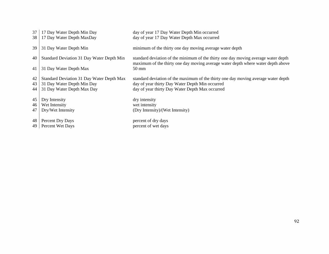
92
37 17 Day Water Depth Min Day day of year 17 Day Water Depth Min occurred
38 17 Day Water Depth MaxDay day of year 17 Day Water Depth Max occurred
39 31 Day Water Depth Min minimum of the thirty one day moving average water depth
40 Standard Deviation 31 Day Water Depth Min standard deviation of the minimum of the thirty one day moving average water depth
41 31 Day Water Depth Max
maximum of the thirty one day moving average water depth where water depth above
50 mm
42 Standard Deviation 31 Day Water Depth Max standard deviation of the maximum of the thirty one day moving average water depth
43 31 Day Water Depth Min Day day of year thirty Day Water Depth Min occurred
44 31 Day Water Depth Max Day day of year thirty Day Water Depth Max occurred
45 Dry Intensity dry intensity
46 Wet Intensity wet intensity
47 Dry/Wet Intensity (Dry Intensity)/(Wet Intensity)
48 Percent Dry Days percent of dry days
49 Percent Wet Days percent of wet days
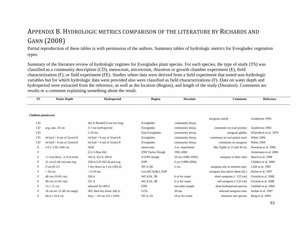
93
APPENDIX B. HYDROLOGIC METRICS COMPARISON OF THE LITERATURE BY RICHARDS AND
GANN (2008) Partial reproduction of these tables is with permission of the authors. Summary tables of hydrologic metrics for Everglades vegetation
types.
Summary of the literature review of hydrologic regimes for Everglades plant species. For each species, the type of study (TS) was
classified as a community description (CD), mesocosm, microcosm, rhizotron or growth chamber experiment (E), field
characterization (F), or field experiment (FE). Studies where data were derived from a field experiment that tested non-hydrologic
variables but for which hydrologic data were provided also were classified as field characterizations (F). Data on water depth and
hydroperiod were extracted from the reference, as well as the location (Region), and length of the study (Duration). Comments are
results or a comment explaining something about the result.
TS Water Depth Hydroperiod Region Duration Comments Reference
Cladium jamaicense
CD dry to flooded if not too long Everglades community descp.
sawgrass marsh Gunderson 1994
CD avg. ann. 10 cm 3-7 mo hydroperiod Everglades community descp. comments on marl prairies Gunderson 1994
CD 5-10 mo East Everglades community descp. sawgrass glades Hilsenbeck et al. 1979
CD rel hyd = 6 out of 1(wet)-8 rel hyd = 6 out of 1(wet)-8 Everglades community descp. comments on wet prairie marl White 1994
CD rel hyd = 4 out of 1(wet)-8 rel hyd = 4 out of 1(wet)-8 Everglades community descp. comments on sawgrass White 1994
E 5/15, 5/30, 5/60 cm 365d mesocosm 2 yr. experiment like Typha at 15 and 30 cm Newman et al. 1996
F (2-) 5-9mo (lit) ENP Taylor Slough 1961-2002 Armentano et al. 2006
F .1-.4 m (dry), .3-.8 m (wet) 343 d, 312 d, 294 d N ENP slough 10 yrs (1985-1995) sawgrass in drier sites Busch et al. 1998
F 21 cm (5-64 cm) ann avg 258 d (135-365 d) ann avg ENP 6 yrs (1998-2004) Childers et al. 2006
F 5 cm (0-11) 1 dry down in 2 yrs (365 d) WCA 2B 2 yrs. sawgrass site in nutrient expt. Craft et al. 1995
F < 50 cm < 6-10 mo Lox,WCA2&3, ENP sawgrass less above these (lit.) Doren et al. 1997
F 48 cm (10-81 cm) 356 d WCA3A, 3B 6 yr for water short sawgrass (< 125 cm) Givnish et al. 2008
F 49 cm (11-81 cm) 357 d WCA3A, 3B 6 yr for water tall sawgrass (>125 cm) Givnish et al. 2008
F 13 ± 11 cm selected 30-180 d ENP one-time sample short hydroperiod species Gottlieb et al. 2006
F 18 cm est. (2-38 cm range) 365, then dry down 2nd yr LOX 30 mo. selected sawgrass sites Jordan et al. 1997
F 46.4 ± 10.4 cm freq < -10 cm, 6.0 ± 0.8% WCA 2A 18 yr for water reference site species King et al. 2004
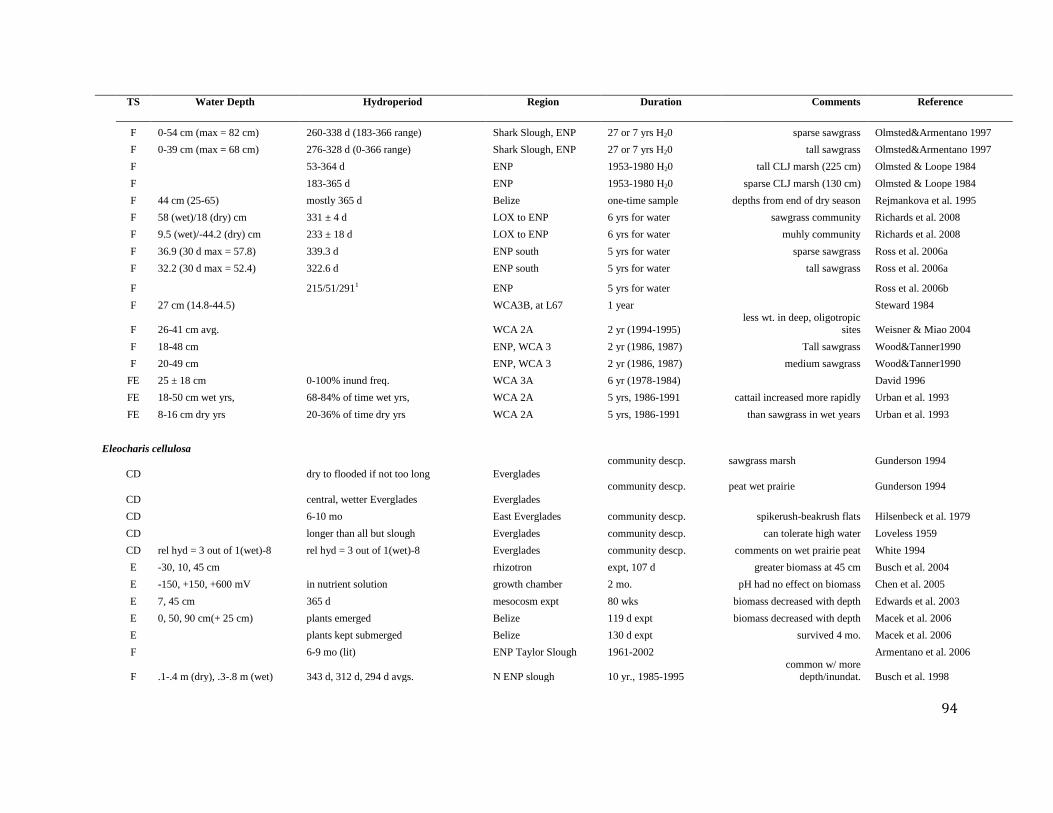
94
TS Water Depth Hydroperiod Region Duration Comments Reference
F 0-54 cm (max = 82 cm) 260-338 d (183-366 range) Shark Slough, ENP 27 or 7 yrs H20 sparse sawgrass Olmsted&Armentano 1997
F 0-39 cm (max = 68 cm) 276-328 d (0-366 range) Shark Slough, ENP 27 or 7 yrs H20 tall sawgrass Olmsted&Armentano 1997
F 53-364 d ENP 1953-1980 H20 tall CLJ marsh (225 cm) Olmsted & Loope 1984
F 183-365 d ENP 1953-1980 H20 sparse CLJ marsh (130 cm) Olmsted & Loope 1984
F 44 cm (25-65) mostly 365 d Belize one-time sample depths from end of dry season Rejmankova et al. 1995
F 58 (wet)/18 (dry) cm 331 ± 4 d LOX to ENP 6 yrs for water sawgrass community Richards et al. 2008
F 9.5 (wet)/-44.2 (dry) cm 233 ± 18 d LOX to ENP 6 yrs for water muhly community Richards et al. 2008
F 36.9 (30 d max = 57.8) 339.3 d ENP south 5 yrs for water sparse sawgrass Ross et al. 2006a
F 32.2 (30 d max = 52.4) 322.6 d ENP south 5 yrs for water tall sawgrass Ross et al. 2006a
F 215/51/2911 ENP 5 yrs for water Ross et al. 2006b
F 27 cm (14.8-44.5) WCA3B, at L67 1 year Steward 1984
F 26-41 cm avg. WCA 2A 2 yr (1994-1995) less wt. in deep, oligotropic
sites Weisner & Miao 2004
F 18-48 cm ENP, WCA 3 2 yr (1986, 1987) Tall sawgrass Wood&Tanner1990
F 20-49 cm ENP, WCA 3 2 yr (1986, 1987) medium sawgrass Wood&Tanner1990
FE 25 ± 18 cm 0-100% inund freq. WCA 3A 6 yr (1978-1984) David 1996
FE 18-50 cm wet yrs, 68-84% of time wet yrs, WCA 2A 5 yrs, 1986-1991 cattail increased more rapidly Urban et al. 1993
FE 8-16 cm dry yrs 20-36% of time dry yrs WCA 2A 5 yrs, 1986-1991 than sawgrass in wet years Urban et al. 1993
Eleocharis cellulosa
CD dry to flooded if not too long Everglades
community descp. sawgrass marsh Gunderson 1994
CD central, wetter Everglades Everglades
community descp. peat wet prairie Gunderson 1994
CD 6-10 mo East Everglades community descp. spikerush-beakrush flats Hilsenbeck et al. 1979
CD longer than all but slough Everglades community descp. can tolerate high water Loveless 1959
CD rel hyd = 3 out of 1(wet)-8 rel hyd = 3 out of 1(wet)-8 Everglades community descp. comments on wet prairie peat White 1994
E -30, 10, 45 cm rhizotron expt, 107 d greater biomass at 45 cm Busch et al. 2004
E -150, +150, +600 mV in nutrient solution growth chamber 2 mo. pH had no effect on biomass Chen et al. 2005
E 7, 45 cm 365 d mesocosm expt 80 wks biomass decreased with depth Edwards et al. 2003
E 0, 50, 90 cm(+ 25 cm) plants emerged Belize 119 d expt biomass decreased with depth Macek et al. 2006
E plants kept submerged Belize 130 d expt survived 4 mo. Macek et al. 2006
F 6-9 mo (lit) ENP Taylor Slough 1961-2002 Armentano et al. 2006
F .1-.4 m (dry), .3-.8 m (wet) 343 d, 312 d, 294 d avgs. N ENP slough 10 yr., 1985-1995
common w/ more
depth/inundat. Busch et al. 1998
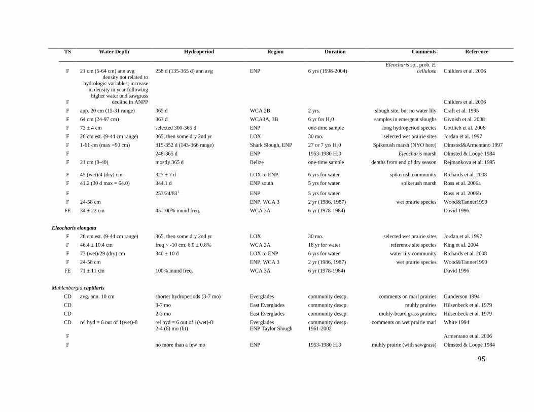
95
TS Water Depth Hydroperiod Region Duration Comments Reference
F 21 cm (5-64 cm) ann avg 258 d (135-365 d) ann avg ENP 6 yrs (1998-2004)
Eleocharis sp., prob. E.
cellulosa Childers et al. 2006
F
density not related to hydrologic variables; increase
in density in year following
higher water and sawgrass decline in ANPP Childers et al. 2006
F app. 20 cm (15-31 range) 365 d WCA 2B 2 yrs. slough site, but no water lily Craft et al. 1995
F 64 cm (24-97 cm) 363 d WCA3A, 3B 6 yr for H20 samples in emergent sloughs Givnish et al. 2008
F 73 ± 4 cm selected 300-365 d ENP one-time sample long hydroperiod species Gottlieb et al. 2006
F 26 cm est. (9-44 cm range) 365, then some dry 2nd yr LOX 30 mo. selected wet prairie sites Jordan et al. 1997
F 1-61 cm (max =90 cm) 315-352 d (143-366 range) Shark Slough, ENP 27 or 7 yrs H20 Spikerush marsh (NYO here) Olmsted&Armentano 1997
F 248-365 d ENP 1953-1980 H20 Eleocharis marsh Olmsted & Loope 1984
F 21 cm (0-40) mostly 365 d Belize one-time sample depths from end of dry season Rejmankova et al. 1995
F 45 (wet)/4 (dry) cm 327 ± 7 d LOX to ENP 6 yrs for water spikerush community Richards et al. 2008
F 41.2 (30 d max = 64.0) 344.1 d ENP south 5 yrs for water spikerush marsh Ross et al. 2006a
F 253/24/831 ENP 5 yrs for water Ross et al. 2006b
F 24-58 cm ENP, WCA 3 2 yr (1986, 1987) wet prairie species Wood&Tanner1990
FE 34 ± 22 cm 45-100% inund freq. WCA 3A 6 yr (1978-1984) David 1996
Eleocharis elongata
F 26 cm est. (9-44 cm range) 365, then some dry 2nd yr LOX 30 mo. selected wet prairie sites Jordan et al. 1997
F 46.4 ± 10.4 cm freq < -10 cm, 6.0 ± 0.8% WCA 2A 18 yr for water reference site species King et al. 2004
F 73 (wet)/29 (dry) cm 340 ± 10 d LOX to ENP 6 yrs for water water lily community Richards et al. 2008
F 24-58 cm ENP, WCA 3 2 yr (1986, 1987) wet prairie species Wood&Tanner1990
FE 71 ± 11 cm 100% inund freq. WCA 3A 6 yr (1978-1984) David 1996
Muhlenbergia capillaris
CD avg. ann. 10 cm shorter hydroperiods (3-7 mo) Everglades community descp. comments on marl prairies Gunderson 1994
CD 3-7 mo East Everglades community descp. muhly prairies Hilsenbeck et al. 1979
CD 2-3 mo East Everglades community descp. muhly-beard grass prairies Hilsenbeck et al. 1979
CD rel hyd = 6 out of 1(wet)-8 rel hyd = 6 out of 1(wet)-8 Everglades community descp. comments on wet prairie marl White 1994
F
2-4 (6) mo (lit) ENP Taylor Slough 1961-2002
Armentano et al. 2006
F no more than a few mo ENP 1953-1980 H20 muhly prairie (with sawgrass) Olmsted & Loope 1984
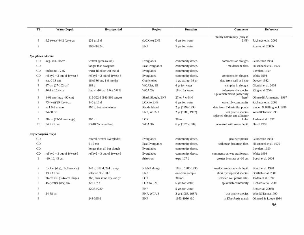
96
TS Water Depth Hydroperiod Region Duration Comments Reference
F 9.5 (wet)/-44.2 (dry) cm 233 ± 18 d (LOX to) ENP 6 yrs for water
muhly community (only in
ENP) Richards et al. 2008
F 198/49/2241 ENP 5 yrs for water Ross et al. 2006b
Nymphaea odorata
CD avg. ann. 30 cm wettest (year-round) Everglades community descp. comments on sloughs Gunderson 1994
CD longer than sawgrass East Everglades community descp. maidencane flats Hilsenbeck et al. 1979
CD inches to 1-2 ft. water filled or wet 365 d Everglades community descp. Loveless 1959
CD rel hyd = 2 out of 1(wet)-8 rel hyd = 2 out of 1(wet)-8 Everglades community descp. comments on sloughs White 1994
F est. 0-38 cm. 16 of 36 yrs, 1-9 mo dry Okefenokee 1 yr, extrap. 36 yr data from well at 1 site Duever 1982
F 67 cm (27-102 cm) 363 d WCA3A, 3B 6 yr for water samples in sloughs Givnish et al. 2008
F 46.4 ± 10.4 cm freq < -10 cm, 6.0 ± 0.8 % WCA 2A 18 yr for water reference site species King et al. 2004
F 1-61 cm (max =90 cm) 315-352 d (143-366 range) Shark Slough, ENP 27 or 7 yr H20
Spikerush marsh (water lily
here) Olmsted&Armentano 1997
F 73 (wet)/29 (dry) cm 340 ± 10 d LOX to ENP 6 yrs for water water lily community Richards et al. 2008
F to 1.9-2 m max 365 d, but have winter Rhode Island 2 yr (1992-1993) data from 7 dissimilar ponds Sinden & Killingbeck 1996
F 24-58 cm ENP, WCA 3 2 yr (1986, 1987) wet prairie species Wood&Tanner1990
F 38 cm (19-52 cm range) 365 d LOX 30 mo.
selected slough and alligator
holes Jordan et al. 1997
FE 54 ± 21 cm 63-100% inund freq. WCA 3A 6 yr (1978-1984) increased with water depth David 1996
Rhynchospora tracyi
CD central, wetter Everglades Everglades community descp. peat wet prairie Gunderson 1994
CD 6-10 mo East Everglades community descp. spikerush-beakrush flats Hilsenbeck et al. 1979
CD longer than all but slough Everglades community descp. Loveless 1959
CD rel hyd = 3 out of 1(wet)-8 rel hyd = 3 out of 1(wet)-8 Everglades community descp. comments on wet prairie peat White 1994
E -30, 10, 45 cm rhizotron expt, 107 d greater biomass at -30 cm Busch et al. 2004
F .1-.4 m (dry), .3-.8 m (wet) 343 d, 312 d, 294 d avgs. N ENP slough 10 yr., 1985-1995 weak correlation with depth Busch et al. 1998
F 13 ± 11 cm selected 30-180 d ENP one-time sample short hydroperiod species Gottlieb et al. 2006
F 26 cm est. (9-44 cm range) 365, then some dry 2nd yr LOX 30 mo. selected wet prairie sites Jordan et al. 1997
F 45 (wet)/4 (dry) cm 327 ± 7 d LOX to ENP 6 yrs for water spikerush community Richards et al. 2008
F 220/51/2201 ENP 5 yrs for water Ross et al. 2006b
F 24-58 cm ENP, WCA 3 2 yr (1986, 1987) wet prairie species Wood&Tanner1990
F 248-365 d ENP 1953-1980 H20 in Eleocharis marsh Olmsted & Loope 1984
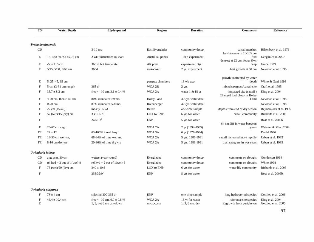
97
TS Water Depth Hydroperiod Region Duration Comments Reference
Typha domingensis
CD 3-10 mo East Everglades community descp. cattail marshes Hilsenbeck et al. 1979
E 15-105; 30-90; 45-75 cm 2 wk fluctuations in level Australia; ponds 100 d experiment
less biomass in 15-105 cm
flux Deegan et al. 2007
E -5 to 115 cm 365 d, but temperate AR pond experiment, 3yr
densest at 22 cm; fewer flws
deep Grace 1989
E 5/15, 5/30, 5/60 cm 365d mesocosm 2 yr. experiment best growth at 60 cm Newman et al. 1996
E 5, 25, 45, 65 cm perspex chambers 18 wk expt
growth unaffected by water
depth White & Ganf 1998
F 5 cm (3-31 cm range) 365 d WCA 2B 2 yrs. mixed sawgrass/cattail site Craft et al. 1995
F 35.7 ± 8.3 cm freq < -10 cm, 3.1 ± 0.4 % WCA 2A water 1 & 18 yr impacted site (cattail ) King et al. 2004
F < 20 cm, then > 60 cm 80% inundated >9 mo Holey Land 4-5 yr. water data
Changed hydrology in Holey
Land Newman et al. 1998
F 0-20 cm 81% inundated 5-8 mo. Rotenberger 4-5 yr. water data Newman et al. 1998
F 27 cm (15-45) mostly 365 d Belize one-time sample depths from end of dry season Rejmankova et al. 1995
F 57 (wet)/15 (dry) cm 338 ± 6 d LOX to ENP 6 yrs for water cattail community Richards et al. 2008
F 242/1/21 ENP 5 yrs for water Ross et al. 2006b
F 26-67 cm avg. WCA 2A 2 yr (1994-1995)
64 cm diff in water between
years Weisner & Miao 2004
FE 24 ± 12 63-100% inund freq. WCA 3A 6 yr (1978-1984) David 1996
FE 18-50 cm wet yrs, 68-84% of time wet yrs, WCA 2A 5 yrs, 1986-1991 cattail increased more rapidly Urban et al. 1993
FE 8-16 cm dry yrs 20-36% of time dry yrs WCA 2A 5 yrs, 1986-1991 than sawgrass in wet years Urban et al. 1993
Utricularia foliosa
CD avg. ann. 30 cm wettest (year-round) Everglades community descp. comments on sloughs Gunderson 1994
CD rel hyd = 2 out of 1(wet)-8 rel hyd = 2 out of 1(wet)-8 Everglades community descp. comments on sloughs White 1994
F 73 (wet)/29 (dry) cm 340 ± 10 d LOX to ENP 6 yrs for water water lily community Richards et al. 2008
F 258/32/91 ENP 5 yrs for water Ross et al. 2006b
Utricularia purpurea
F 73 ± 4 cm selected 300-365 d ENP one-time sample long hydroperiod species Gottlieb et al. 2006
F 46.4 ± 10.4 cm freq < -10 cm, 6.0 ± 0.8 % WCA 2A 18 yr for water reference site species King et al. 2004
E 1, 3, not 8 mo dry-down microcosm 1, 3, 8 mo. dry Regrowth from periphyton Gottlieb et al. 2005
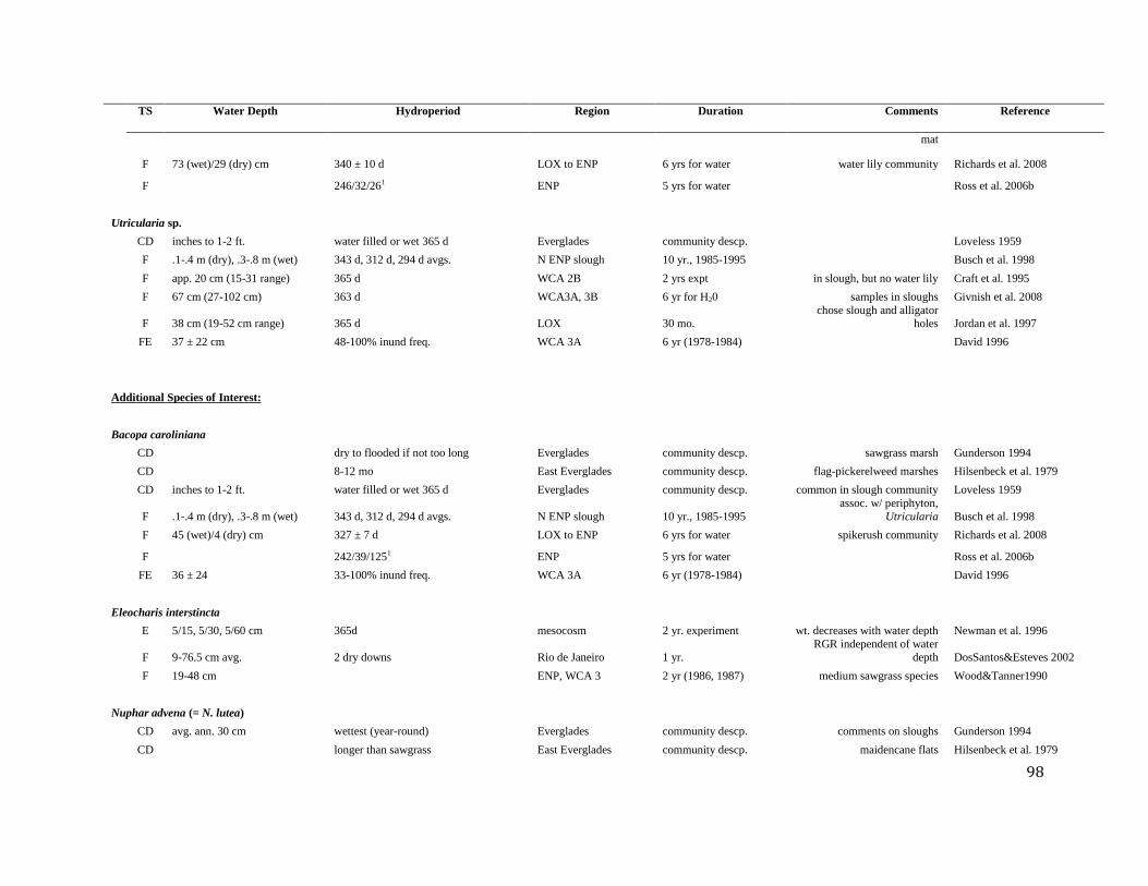
98
TS Water Depth Hydroperiod Region Duration Comments Reference
mat
F 73 (wet)/29 (dry) cm 340 ± 10 d LOX to ENP 6 yrs for water water lily community Richards et al. 2008
F 246/32/261 ENP 5 yrs for water Ross et al. 2006b
Utricularia sp.
CD inches to 1-2 ft. water filled or wet 365 d Everglades community descp. Loveless 1959
F .1-.4 m (dry), .3-.8 m (wet) 343 d, 312 d, 294 d avgs. N ENP slough 10 yr., 1985-1995 Busch et al. 1998
F app. 20 cm (15-31 range) 365 d WCA 2B 2 yrs expt in slough, but no water lily Craft et al. 1995
F 67 cm (27-102 cm) 363 d WCA3A, 3B 6 yr for H20 samples in sloughs Givnish et al. 2008
F 38 cm (19-52 cm range) 365 d LOX 30 mo. chose slough and alligator
holes Jordan et al. 1997
FE 37 ± 22 cm 48-100% inund freq. WCA 3A 6 yr (1978-1984) David 1996
Additional Species of Interest:
Bacopa caroliniana
CD dry to flooded if not too long Everglades community descp. sawgrass marsh Gunderson 1994
CD 8-12 mo East Everglades community descp. flag-pickerelweed marshes Hilsenbeck et al. 1979
CD inches to 1-2 ft. water filled or wet 365 d Everglades community descp. common in slough community Loveless 1959
F .1-.4 m (dry), .3-.8 m (wet) 343 d, 312 d, 294 d avgs. N ENP slough 10 yr., 1985-1995
assoc. w/ periphyton,
Utricularia Busch et al. 1998
F 45 (wet)/4 (dry) cm 327 ± 7 d LOX to ENP 6 yrs for water spikerush community Richards et al. 2008
F 242/39/1251 ENP 5 yrs for water Ross et al. 2006b
FE 36 ± 24 33-100% inund freq. WCA 3A 6 yr (1978-1984) David 1996
Eleocharis interstincta
E 5/15, 5/30, 5/60 cm 365d mesocosm 2 yr. experiment wt. decreases with water depth Newman et al. 1996
F 9-76.5 cm avg. 2 dry downs Rio de Janeiro 1 yr.
RGR independent of water
depth DosSantos&Esteves 2002
F 19-48 cm ENP, WCA 3 2 yr (1986, 1987) medium sawgrass species Wood&Tanner1990
Nuphar advena (= N. lutea)
CD avg. ann. 30 cm wettest (year-round) Everglades community descp. comments on sloughs Gunderson 1994
CD longer than sawgrass East Everglades community descp. maidencane flats Hilsenbeck et al. 1979
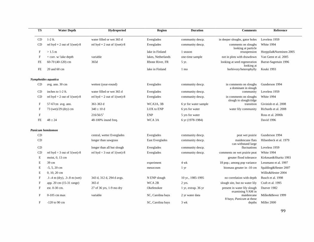
99
TS Water Depth Hydroperiod Region Duration Comments Reference
CD 1-2 ft. water filled or wet 365 d Everglades community descp. in deeper sloughs, gator holes Loveless 1959
CD rel hyd = 2 out of 1(wet)-8 rel hyd = 2 out of 1(wet)-8 Everglades community descp. comments on sloughs White 1994
F > 1.5 m lake in Finland 1 season looking at particle
resuspension Horppila&Nurminen 2005
F + corr. w/ lake depth variable lakes, Netherlands one-time sample not in plots with drawdown Van Geest et al. 2005
FE 60-70 (40-120) cm 365d Rhone River, FR 5 yr. looking at seed regeneration Barrat-Sagretain 1996
FE 20 and 60 cm lake in Finland 1 mo looking at
herbivory/heterophylly Kouki 1993
Nymphoides aquatica
CD avg. ann. 30 cm wettest (year-round) Everglades community descp. in comments on sloughs Gunderson 1994
CD inches to 1-2 ft. water filled or wet 365 d Everglades community descp. a dominant in slough
community Loveless 1959
CD rel hyd = 2 out of 1(wet)-8 rel hyd = 2 out of 1(wet)-8 Everglades community descp. in comments on sloughs White 1994
F 57-67cm avg. ann. 361-363 d WCA3A, 3B 6 yr for water sample
slough to slough/ridge
transition Givinish et al. 2008
F 73 (wet)/29 (dry) cm 340 ± 10 d LOX to ENP 6 yrs for water water lily community Richards et al. 2008
F 216/56/51 ENP 5 yrs for water Ross et al. 2006b
FE 48 ± 24 48-100% inund freq. WCA 3A 6 yr (1978-1984) David 1996
Panicum hemitomon
CD central, wetter Everglades Everglades community descp. peat wet prairie Gunderson 1994
CD longer than sawgrass East Everglades community descp. maidencane flats Hilsenbeck et al. 1979
CD longer than all but slough Everglades community descp.
can withstand large
fluctuations Loveless 1959
CD rel hyd = 3 out of 1(wet)-8 rel hyd = 3 out of 1(wet)-8 Everglades community descp. comments on wet prairie peat White 1994
E moist, 0, 13 cm greater flood tolerance Kirkman&Sharitz 1993
E 39 cm experiment 4 wk 18 pop.; among pop variance Lessmann et al. 1997
E -5, 5, 20 cm mesocosm 1 yr biomass greater in -10 cm Spalding&Hester 2007
E 0, 10, 20 cm Willis&Hester 2004
F .1-.4 m (dry), .3-.8 m (wet) 343 d, 312 d, 294 d avgs. N ENP slough 10 yr., 1985-1995 no correlation with depth Busch et al. 1998
F app. 20 cm (15-31 range) 365 d WCA 2B 2 yrs. slough site, but no water lily Craft et al. 1995
F est. 0-30 cm. 27 of 36 yrs, 1-9 mo dry Okefenokee 1 yr, extrap. 36 yr present in water lily slough Duever 1982
F 0-105 cm max variable SC, Carolina bays 2 yr water data
examining VAM in
maidencane Miller&Bever 1999
F -120 to 90 cm SC, Carolina bays 3 wk 8 bays; Panicum at these
depths Miller 2000
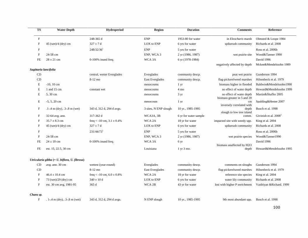
100
TS Water Depth Hydroperiod Region Duration Comments Reference
F 248-365 d ENP 1953-80 for water in Eleocharis marsh Olmsted & Loope 1984
F 45 (wet)/4 (dry) cm 327 ± 7 d LOX to ENP 6 yrs for water spikerush community Richards et al. 2008
F 248/32/361 ENP 5 yrs for water Ross et al. 2006b
F 24-58 cm ENP, WCA 3 2 yr (1986, 1987) wet prairie site Wood&Tanner 1990
FE 28 ± 21 cm 0-100% inund freq. WCA 3A 6 yr (1978-1984) David 1996
negatively affected by depth Mckee&Mendelssohn 1989
Sagittaria lancifolia
CD central, wetter Everglades Everglades community descp. peat wet prairie Gunderson 1994
CD 8-12 mo East Everglades community descp. flag-pickerelweed marshes Hilsenbeck et al. 1979
E -10, 10 cm mesocosms 1 yr biomass higher in flooded Baldwin&Mendelssohn1998
E 1 and 15 cm constant wet mesocosms 4 mo no effect of water depth Howard&Mendelssohn 1999
E 5, 30 cm mesocosms 3 yr no effect of water depth Martin&Shaffer 2005
E -5, 5, 20 cm mesocosm 1 yr
biomass greater in 5 and 20
cm Spalding&Hester 2007
F .1-.4 m (dry), .3-.8 m (wet) 343 d, 312 d, 294 d avgs. 3 sites, N ENP slough 10 yr., 1985-1995
inversely correlated with
depth Busch et al. 1998
F 32-64 avg. ann. 317-362 d WCA3A, 3B 6 yr for water sample slough to low tree island
comm. Givinish et al. 20083
F 35.7 ± 8.3 cm freq < -10 cm, 3.1 ± 0.4% WCA 2A 18 yr for water impacted site with weedy spp. King et al. 2004
F 45 (wet)/4 (dry) cm 327 ± 7 d LOX to ENP 6 yrs for water spikerush community Richards et al. 2008
F 231/44/731 ENP 5 yrs for water Ross et al. 2006b
F 24-58 cm ENP, WCA 3 2 yr (1986, 1987) wet prairie species Wood&Tanner1990
FE 24 ± 18 cm 0-100% inund freq. WCA 3A 6 yr David 1996
FE est. 15, 22.5, 30 cm Louisiana 1 yr 3 mo.
biomass unaffected by H2O
depth Howard&Mendelssohn 1995
Utricularia gibba (= U. biflora, U. fibrosa)
CD avg. ann. 30 cm wettest (year-round) Everglades community descp. comments on sloughs Gunderson 1994
CD 8-12 mo East Everglades community descp. flag-pickerelweed marshes Hilsenbeck et al. 1979
F 46.4 ± 10.4 cm freq < -10 cm, 6.0 ± 0.8% WCA 2A 18 yr for water reference site species King et al. 2004
F 73 (wet)/29 (dry) cm 340 ± 10 d LOX to ENP 6 yrs for water water lily community Richards et al. 2008
F est. 30 cm avg, 1981-95 365 d WCA 2B 43 yr for water lost with higher P enrichment Vaithiyan &Richard. 1999
Chara sp.
F . 1-.4 m (dry), .3-.8 m (wet) 343 d, 312 d, 294 d avgs. N ENP slough 10 yr., 1985-1995 9th most abundant spp. Busch et al. 1998
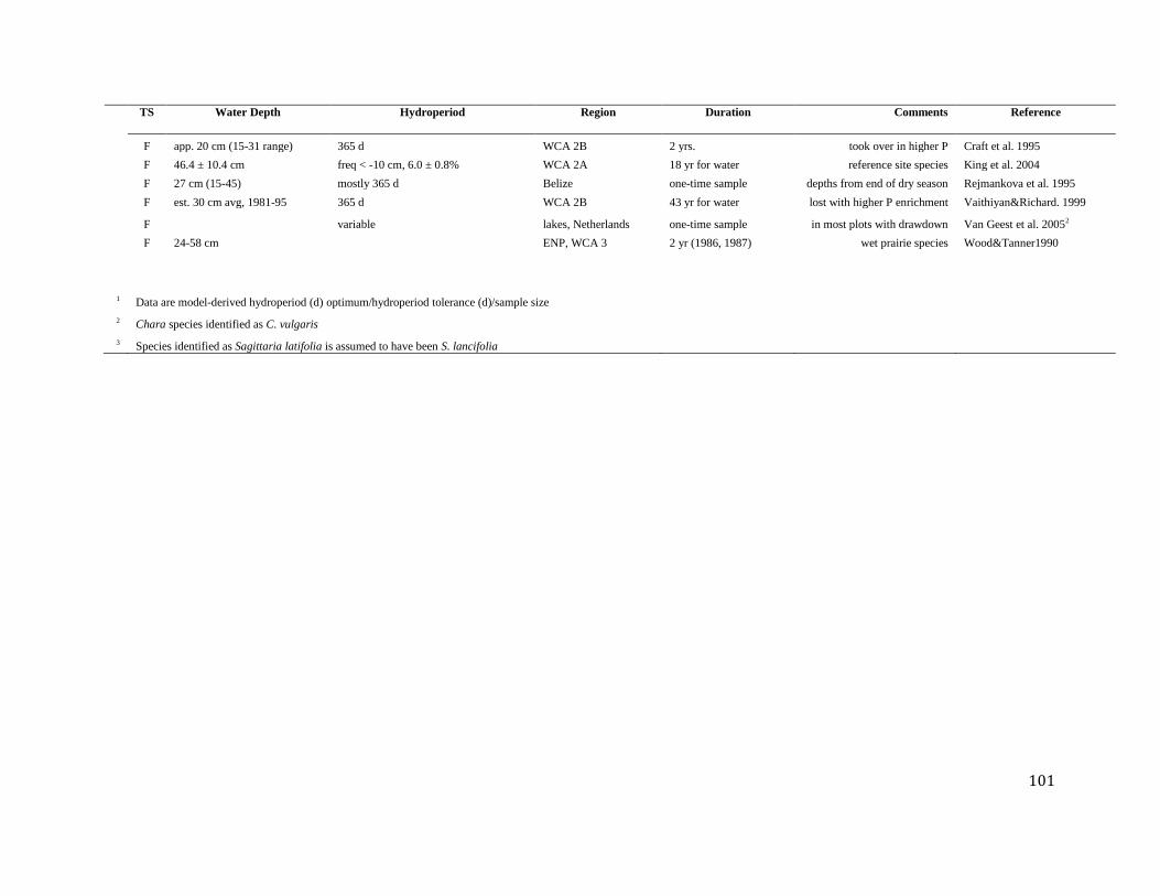
101
TS Water Depth Hydroperiod Region Duration Comments Reference
F app. 20 cm (15-31 range) 365 d WCA 2B 2 yrs. took over in higher P Craft et al. 1995
F 46.4 ± 10.4 cm freq < -10 cm, 6.0 ± 0.8% WCA 2A 18 yr for water reference site species King et al. 2004
F 27 cm (15-45) mostly 365 d Belize one-time sample depths from end of dry season Rejmankova et al. 1995
F est. 30 cm avg, 1981-95 365 d WCA 2B 43 yr for water lost with higher P enrichment Vaithiyan&Richard. 1999
F variable lakes, Netherlands one-time sample in most plots with drawdown Van Geest et al. 20052
F 24-58 cm ENP, WCA 3 2 yr (1986, 1987) wet prairie species Wood&Tanner1990
1 Data are model-derived hydroperiod (d) optimum/hydroperiod tolerance (d)/sample size
2 Chara species identified as C. vulgaris
3 Species identified as Sagittaria latifolia is assumed to have been S. lancifolia
102
Reference List for Appendix B Summary Table
Armentano, T. V., J. P. Sah, M. S. Ross, D. T. Jones, H. C. Cooley and C. S. Smith. 2006.
Rapid responses of vegetation to hydrological changes in Taylor Slough, Everglades National
Park, Florida, USA. Hydrobiologia 569: 293-309.
Baldwin, A. H. and I. A. Mendelssohn. 1998. Effects of salinity and water level on coastal
marshes: an experimental test of disturbance as a catalyst for vegetation change. Aquatic
Botany 61: 255-268.
Barrat-Segretain, M. H. 1996. Germination and colonisation dynamics of Nuphar lutea (L) Sm
in a former river channel. Aquatic Botany 55: 31-38.
Busch, D. E., W. F. Loftus and O. L. Bass. 1998. Long-term hydrologic effects on marsh
plant community structure in the southern Everglades. Wetlands 18: 230-241.
Busch J., I. A. Mendelssohn, B. Lorenzen, H. Brix, and S. Miao. 2004. Growth response of the
Everglades wet prairie species Eleocharis cellulosa and Rhyncospora tracyi to water level and
phosphate availability. Aquatic Botany 78: 37 – 54.
Chen, H., I. A. Mendelssohn, B. Lorenzen, H. Brix, and S. Miao. 2005. Growth and nutrient
responses of Eloecharis cellulosa (Cyperaceae) to phosphate level and redox
intensity. American Journal of Botany 92: 1457-1466.
Chen, H. J., I. A. Mendelssohn, B. Lorenzen, H. Brix and S. L. Miao. 2008. Effects of
phosphate availability and redox intensity on growth and nutrient uptake of
Rhynchospora tracyi, a wet prairie species in the everglades. Wetlands 28: 151-163.
Childers, D. L., D. Iwaniec, D. Rondeau, G. Rubio, E. Verdon and C. J. Madden. 2006.
Responses of sawgrass and spikerush to variation in hydrologic drivers and salinity in Southern
Everglades marshes. Hydrobiologia 569: 273-292.
Craft, C. B., J. Vymazal and C. J. Richardson. 1995. Response of Everglades plant
communities to nitrogen and phosphorus additions. Wetlands 15: 258-271.
David, P. G. 1996. Changes in plant communities relative to hydrologic conditions in the
Florida Everglades. Wetlands 16: 15-23.
Deegan, B. M., S. D. White and G. G. Ganf. 2007. The influence of water level fluctuations on
the growth of four emergent macrophyte species. Aquatic Botany 86: 309-315.

103
Doren, R. F., T. V. Armentano, L. D. Whiteaker and R. D. Jones. 1997. Marsh vegetation
patterns and soil phosphorus gradients in the Everglades ecosystem. Aquatic Botany 56: 145-
163.
Dos Santos, A. M. and F. D. Esteves. 2002. Primary production and mortality of Eleocharis
interstincta in response to water level fluctuations. Aquatic Botany 74: 189-199.
Duever, M. J. 1982. Hydrology--plant community relationships in the Okefenokee Swamp.
Florida Scientist 45: 171-176.
Edwards, A. L., D. W. Lee and J. H. Richards. 2003. Responses to a fluctuating
environment: effects of water depth on growth and biomass allocation in Eleocharis
cellulosa Torr. (Cyperaceae). Canadian Journal of Botany 81: 964-975.
Givnish, T. J., J. C. Volin, V. D. Owen, V. C. Volin, J. D. Muss and P. H. Glaser. 2008.
Vegetation differentiation in the patterned landscape of the central Everglades: importance of
local and landscape drivers. Global Ecology and Biogeography 17: 384-402.
Gottlieb, A. G., J. Richards, and E. Gaiser, 2005. Effects of desiccation
duration on the community structure and nutrient retention of short and long hydroperiod
Everglades periphyton mats. Aquatic Botany 82: 99–112.
Gottlieb, A. D., J. H. Richards and E. E. Gaiser. 2006. Comparative study of periphyton
community structure in long and short-hydroperiod Everglades marshes. Hydrobiologia 569:
195-207.
Grace, J. B. 1989. Effects of water depth on Typha latifolia and Typha domingensis. American
Journal of Botany 76: 762-768.
Gunderson, L. H. 1994. Vegetation of the Everglades: Determinants of community
composition. In S. M. Davis and J. C. Ogden [eds.], Everglades, the ecosystem and its
restoration., 323-340. St. Lucie Press, Delray Beach, FL.
Hilsenbeck, C. E., R. H. Hofstetter and T. R. Alexander. 1979. Description of major
plant communities in the east Everglades.
Horppila, J. and L. Nurminen. 2005. Effects of different macrophyte growth forms on
sediment and P resuspension in a shallow lake. Hydrobiologia 545: 167-175.
Howard, R. J. and I. A. Mendelssohn. 1999. Salinity as a constraint on growth of
oligohaline marsh macrophytes. II. Salt pulses and recovery potential. American Journal
of Botany 86: 795-806.
Howard, R. J. and I. A. Mendelssohn. 1995. Effect of increased water depth on growth of a
common perennial freshwater-intermediate marsh species in coastal Louisiana. Wetlands

104
15: 82-91.
Jordan, F., H. L. Jelks and W. M. Kitchens. 1997. Habitat structure and plant community
composition in a northern everglades wetland landscape. Wetlands 17: 275-283.
King, R. S., C. J. Richardson, D. L. Urban and E. A. Romanowicz. 2004. Spatial
dependency of vegetation-environment linkages in an anthropogenically influenced
wetland ecosystem. Ecosystems 7: 75-97.
Kirkman, L. K. and R. R. Sharitz. 1993. Growth in controlled water regimes of three
grassescommon in freshwater wetlands of the southeastern USA. Aquatic botany 44: 345-359.
Kouki, J. 1993. Herbivory Modifies the Production of Different Leaf Types in the Yellow
Water-Lily, Nuphar-Lutea (Nymphaeaceae). Functional Ecology 7: 21-26.
Lessmann, J. M., I. A. Mendelssohn, M. W. Hester and K. L. Mckee. 1997. Population
variation in growth response to flooding of three marsh grasses. Ecological Engineering
8: 31-47.
Lissner, J., I. A. Mendelssohn, B. Lorenzen, H. Brix, K. L. Mckee and S. L. Miao.
2003.Interactive effects of redox intensity and phosphate availability on growth and nutrient
relations of Cladium jamaicense (Cyperaceae). American Journal of Botany 90: 736-748.
Loveless, C. M. 1959. A study of the vegetation in the Florida Everglades. Ecology 40: 1-9.
Macek, P., E. Rejmankova and K. Houdkova. 2006. The effect of long-term submergence
on functional properties of Eleocharis cellulosa Torr. Aquatic Botany 84: 251-258.21.
Martin, S. B. and G. P. Shaffer. 2005. Sagittaria biomass partitioning relative to salinity,
hydrologic regime, and substrate type: Implications for plant distribution patterns in
Coastal Louisiana, United States. Journal of Coastal Research 21: 167-174.
Mckee, K. L. and Irving A. Mendelssohn. 1989. Response of a freshwater marsh plant
community to increased salinity and increased water level. Aquatic botany 34: 301-316.
Miller, S. P. 2000. Arbuscular mycorrhizal colonization of semi-aquatic grasses along a wide
hydrologic gradient. New Phytologist 145: 145-155.
Miller, S. P. and J. D. Bever. 1999. Distribution of arbuscular mycorrhizal fungi in stands of the
wetland grass Panicum hemitomon along a wide hydrologic gradient. Oecologia 119:
586-592.
Newman, S., J. B. Grace and J. W. Koebel. 1996. Effects of nutrients and hydroperiod on
Typha, Cladium, and Eleocharis: Implications for Everglades restoration. Ecological
Applications 6: 774-783.

105
Newman, S., J. Schuette, J. B. Grace, K. Rutchey, T. Fontaine, K. R. Reddy and M.
Pietrucha. 1998. Factors influencing cattail abundance in the northern Everglades.
Aquatic Botany 60: 265-280.
Olmsted, I. and L. L. Loope. 1984. Plant communities of Everglades National Park. In P. J.
Gleason [ed.], Environments of South Florida: Present and Past II., 167-184. Miami
Geological Society, Coral Gables, FL.
Olmsted, I. and T. V. Armentano. 1997. Vegetation of Shark Slough, Everglades National
Park. South Florida Natural Resources Center, Everglades National Park, Homestead, FL
33035-6733, 97-001.
Pezeshki, S. R., R. D. Delaune, H. K. Kludze and H. S. Choi. 1996. Photosynthetic and
growth responses of cattail (Typha domingensis) and sawgrass (Cladium jamaicense) to
soil redox conditions. Aquatic Botany 54: 25-35.
Rejmankova, E., K. O. Pope, M. D. Pohl and J. M. Reybenayas. 1995. Freshwater wetland plant
communities of Northern Belize - Implications for paleoecological studies of Maya wetland
agriculture. Biotropica 27: 28-36.
Richards, J. H., T. E. Philippi, P. Kalla and D. Scheidt. 2008. Everglades marsh
vegetation: Species associations and spatial distributions from R-EMAP Phase III, 30.
Florida International University and Region IV US EPA.
Ross, M. S., S. Mitchell-Bruker, J. P. Sah, S. Stothoff, P. L. Ruiz, D. L. Reed, K.
Jayachandran and C. L. Coultas. 2006a. Interaction of hydrology and nutrient
limitation in the Ridge and Slough landscape of the southern Everglades. Hydrobiologia
569: 37-59.
Ross, M. S., J. P. Sah, P. L. Ruiz, P. L. Ruiz, D. T. Jones, H. C. Cooley, R. Travieso, F.
Tobias, J. R. Snyder and D. Hagyari. 2006b. Effect of hydrologic restoration on the
habitat of the Cape Sable Seaside sparrow; Annual Report for 2004-2005. Everglades
National Park.
Sinden-Hempstead, M. and K. T. Killingbeck. 1996. Influences of water depth and
substrate nitrogen on leaf surface area and maximum bed extension in Nymphaea
odorata. Aquatic Botany 53: 151-162.
Spalding, E. A. and M. W. Hester. 2007. Interactive effects of hydrology and salinity on
oligohaline plant species productivity: Implications of relative sea-level rise. Estuaries
and Coasts 30: 214-225.
Steward, K. K. 1984. Physiological, edaphic and environmental characteristics of Everglades
sawgrass communities. In P. J. Gleason [ed.], Environments of South Florida: Present

106
and Past II, 157-166. Miami Geological Society, Coral Gables, FL.
Urban, N. H., S. M. Davis and N. G. Aumen. 1993. Fluctuations in sawgrass and cattail
densities in Everglades Water Conservation Area 2A under varying nutrient, hydrologic
and fire regimes. Aquatic Botany 46: 203-223.
Vaithiyanathan, P. and C. J. Richardson. 1999. Macrophyte species changes in the
Everglades: Examination along a eutrophication gradient. Journal of Environmental
Quality 28: 1347-1358.
Van Geest, G. J., H. Coops, R. M. M. Roijackers, A. D. Buijse and M. Scheffer. 2005.
Succession of aquatic vegetation driven by reduced water-level fluctuations in floodplain
lakes. Journal of Applied Ecology 42: 251-260.
Weisner, S. E. B. and S. L. Miao. 2004. Use of morphological variability in Cladium
jamaicense and Typha domingensis to understand vegetation changes in an Everglades
marsh. Aquatic botany 78: 319-335.
White, P. S. 1994. Synthesis: Vegetation pattern and process in the Everglades ecosystem. In S.
M. Davis and J. C. Ogden [eds.], Everglades, the ecosystem and its restoration., 445-458.
St. Lucie Press, Delray Beach, FL.
White, S. D. and G. G. Ganf. 1998. The influence of convective flow on rhizome length in
Typha domingensis over a water depth gradient. Aquatic Botany 62: 57-70.
Willis, J. M. and M. W. Hester. 2004. Interactive effects of salinity, flooding, and soil type
on Panicum hemitomon. Wetlands 24: 43-50.
Wood, J. M. and G. W. Tanner. 1990. Graminoid community composition and structure
within four everglades management areas. Wetlands 10: 127-149.

107
APPENDIX C. HISTOGRAMS OF THE RELATIVE FREQUENCY OF
OCCURRENCE OF BINNED VALUES FOR EACH OF THE MODELED
VARIABLES WITHIN EACH OF THE MAPPED FRESH WATER MARSH
AND WET PRAIRIE VEGETATION CLASSES.
The mapped vegetation classes used in this analysis are described in the text. The frequency
histograms of each metric represent the distribution of values found within the modeled domain
(the WCAs and ENP). The dashed green lines are normal distributions fitted to the mean and
standard deviation of the frequency histograms (blue bars). The solid red lines are skewed
normal distributions fitted to the histograms. The bottom chart presents all the skewed normal
distributions for all the vegetation classes together.
Figures start on next page.
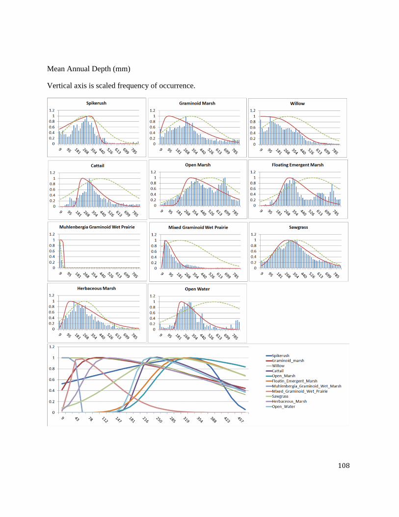
108
Mean Annual Depth (mm)
Vertical axis is scaled frequency of occurrence.
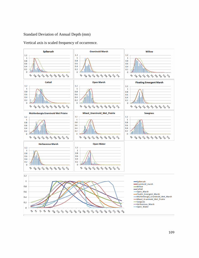
109
Standard Deviation of Annual Depth (mm)
Vertical axis is scaled frequency of occurrence.
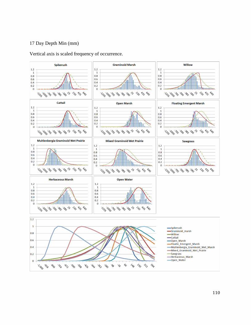
110
17 Day Depth Min (mm)
Vertical axis is scaled frequency of occurrence.
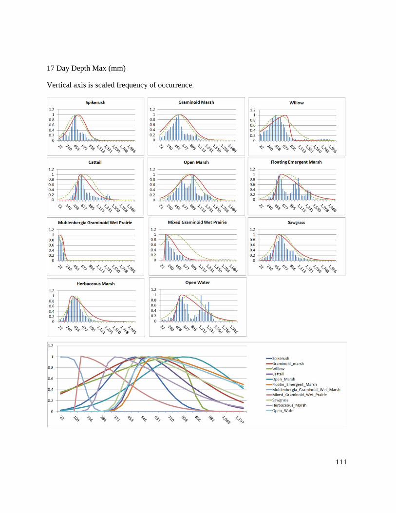
111
17 Day Depth Max (mm)
Vertical axis is scaled frequency of occurrence.
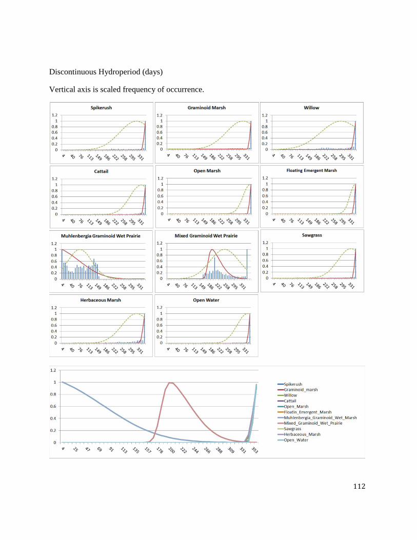
112
Discontinuous Hydroperiod (days)
Vertical axis is scaled frequency of occurrence.
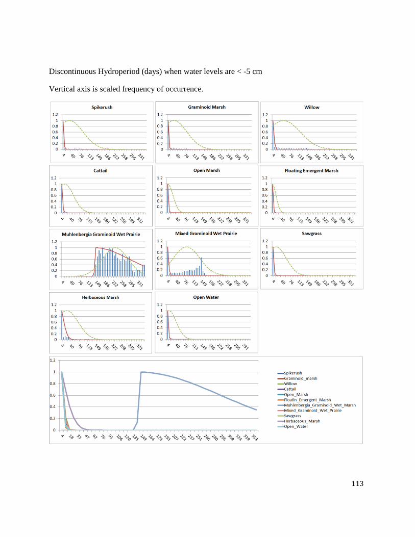
113
Discontinuous Hydroperiod (days) when water levels are < -5 cm
Vertical axis is scaled frequency of occurrence.
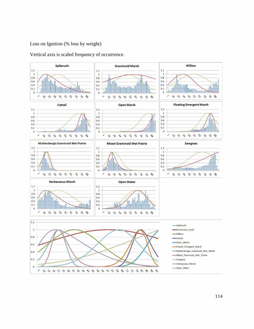
114
Loss on Ignition (% loss by weight)
Vertical axis is scaled frequency of occurrence.
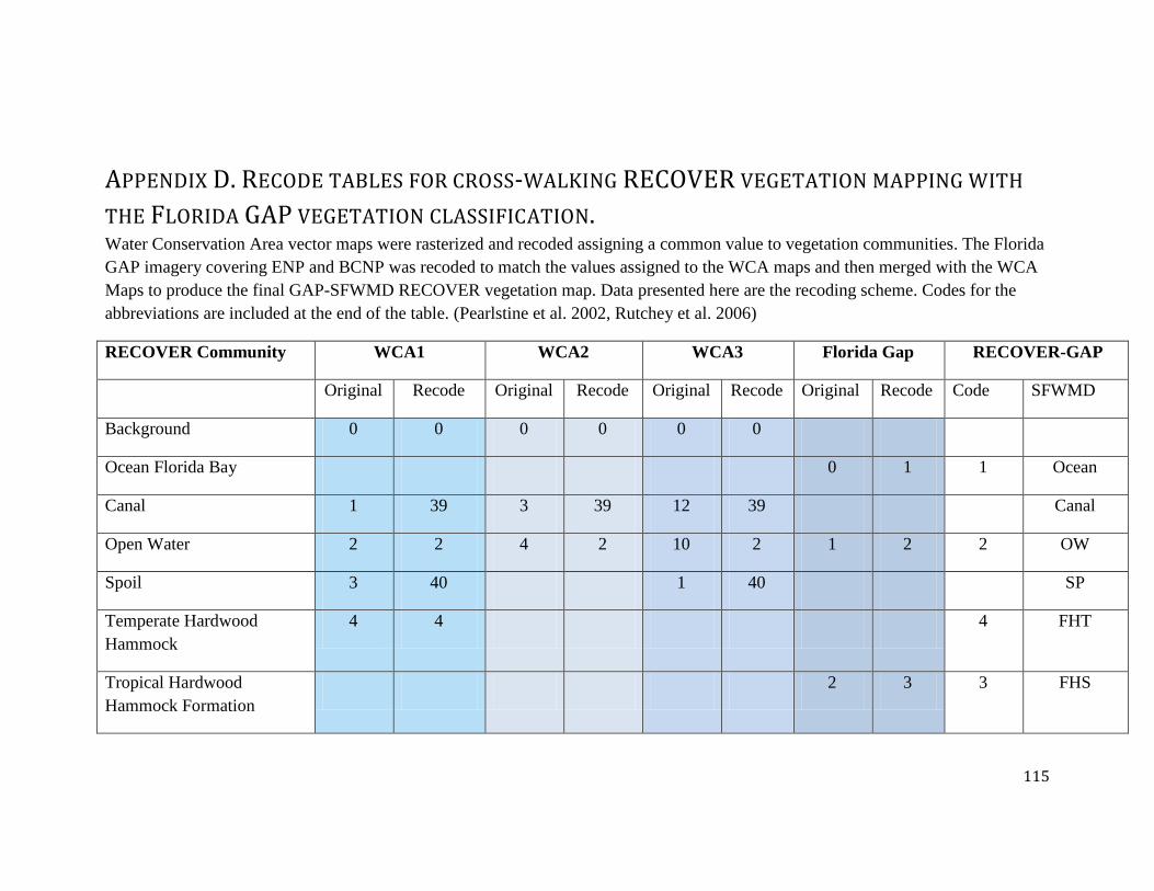
115
APPENDIX D. RECODE TABLES FOR CROSS-WALKING RECOVER VEGETATION MAPPING WITH
THE FLORIDA GAP VEGETATION CLASSIFICATION. Water Conservation Area vector maps were rasterized and recoded assigning a common value to vegetation communities. The Florida
GAP imagery covering ENP and BCNP was recoded to match the values assigned to the WCA maps and then merged with the WCA
Maps to produce the final GAP-SFWMD RECOVER vegetation map. Data presented here are the recoding scheme. Codes for the
abbreviations are included at the end of the table. (Pearlstine et al. 2002, Rutchey et al. 2006)
RECOVER Community WCA1 WCA2 WCA3 Florida Gap RECOVER-GAP
Original Recode Original Recode Original Recode Original Recode Code SFWMD
Background 0 0 0 0 0 0
Ocean Florida Bay 0 1 1 Ocean
Canal 1 39 3 39 12 39 Canal
Open Water 2 2 4 2 10 2 1 2 2 OW
Spoil 3 40 1 40 SP
Temperate Hardwood
Hammock
4 4 4 FHT
Tropical Hardwood
Hammock Formation
2 3 3 FHS
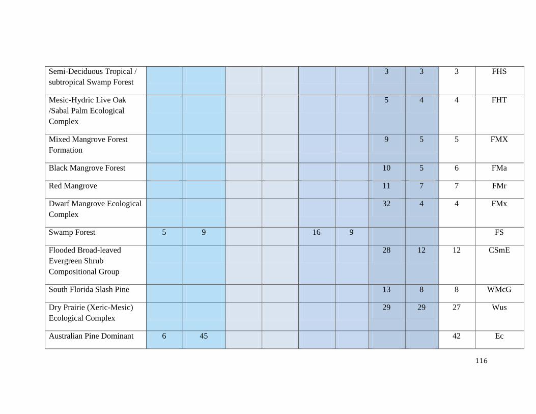
116
Semi-Deciduous Tropical /
subtropical Swamp Forest
3 3 3 FHS
Mesic-Hydric Live Oak
/Sabal Palm Ecological
Complex
5 4 4 FHT
Mixed Mangrove Forest
Formation
9 5 5 FMX
Black Mangrove Forest 10 5 6 FMa
Red Mangrove 11 7 7 FMr
Dwarf Mangrove Ecological
Complex
32 4 4 FMx
Swamp Forest 5 9 16 9 FS
Flooded Broad-leaved
Evergreen Shrub
Compositional Group
28 12 12 CSmE
South Florida Slash Pine 13 8 8 WMcG
Dry Prairie (Xeric-Mesic)
Ecological Complex
29 29 27 Wus
Australian Pine Dominant 6 45 42 Ec
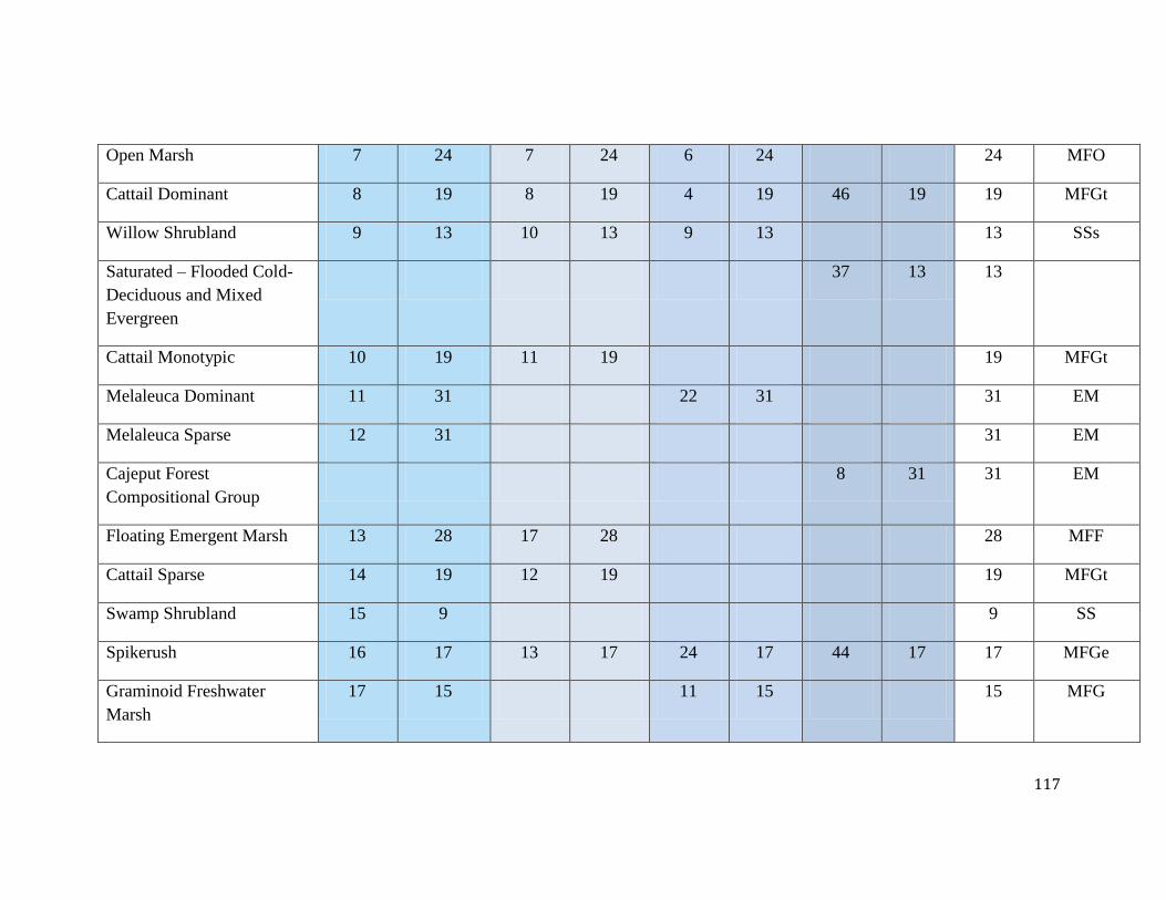
117
Open Marsh 7 24 7 24 6 24 24 MFO
Cattail Dominant 8 19 8 19 4 19 46 19 19 MFGt
Willow Shrubland 9 13 10 13 9 13 13 SSs
Saturated – Flooded Cold-
Deciduous and Mixed
Evergreen
37 13 13
Cattail Monotypic 10 19 11 19 19 MFGt
Melaleuca Dominant 11 31 22 31 31 EM
Melaleuca Sparse 12 31 31 EM
Cajeput Forest
Compositional Group
8 31 31 EM
Floating Emergent Marsh 13 28 17 28 28 MFF
Cattail Sparse 14 19 12 19 19 MFGt
Swamp Shrubland 15 9 9 SS
Spikerush 16 17 13 17 24 17 44 17 17 MFGe
Graminoid Freshwater
Marsh
17 15 11 15 15 MFG
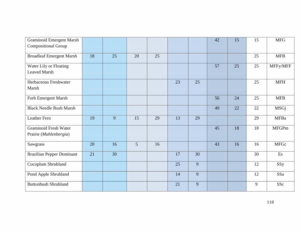
118
Graminoid Emergent Marsh
Compositional Group
42 15 15 MFG
Broadleaf Emergent Marsh 18 25 20 25 25 MFB
Water Lily or Floating
Leaved Marsh
57 25 25 MFFy/MFF
Herbaceous Freshwater
Marsh
23 25 25 MFH
Forb Emergent Marsh 56 24 25 MFB
Black Needle Rush Marsh 49 22 22 MSGj
Leather Fern 19 9 15 29 13 29 29 MFBa
Graminoid Fresh Water
Prairie (Muhlenbergia)
45 18 18 MFGPm
Sawgrass 20 16 5 16 43 16 16 MFGc
Brazilian Pepper Dominant 21 30 17 30 30 Es
Cocoplum Shrubland 25 9 12 SSy
Pond Apple Shrubland 14 9 12 SSa
Buttonbush Shrubland 21 9 9 SSc
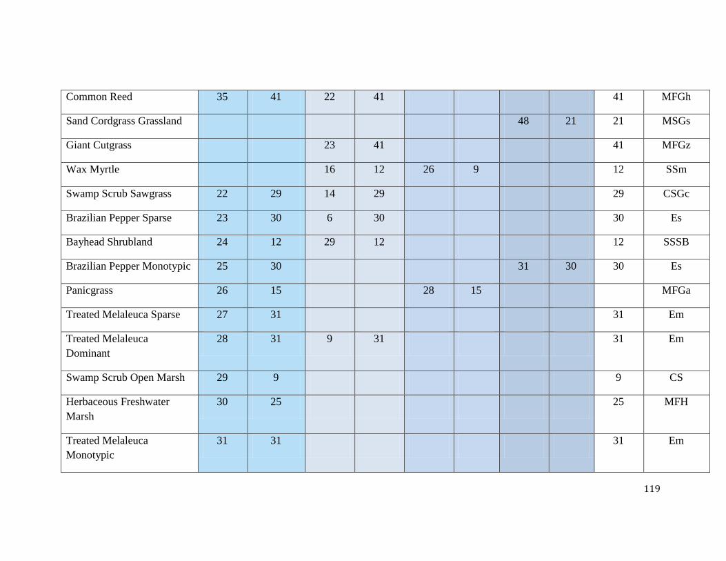
119
Common Reed 35 41 22 41 41 MFGh
Sand Cordgrass Grassland 48 21 21 MSGs
Giant Cutgrass 23 41 41 MFGz
Wax Myrtle 16 12 26 9 12 SSm
Swamp Scrub Sawgrass 22 29 14 29 29 CSGc
Brazilian Pepper Sparse 23 30 6 30 30 Es
Bayhead Shrubland 24 12 29 12 12 SSSB
Brazilian Pepper Monotypic 25 30 31 30 30 Es
Panicgrass 26 15 28 15 MFGa
Treated Melaleuca Sparse 27 31 31 Em
Treated Melaleuca
Dominant
28 31 9 31 31 Em
Swamp Scrub Open Marsh 29 9 9 CS
Herbaceous Freshwater
Marsh
30 25 25 MFH
Treated Melaleuca
Monotypic
31 31 31 Em
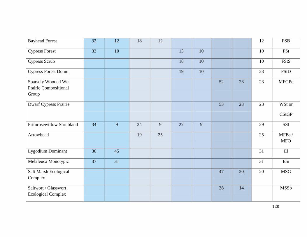
120
Bayhead Forest 32 12 18 12 12 FSB
Cypress Forest 33 10 15 10 10 FSt
Cypress Scrub 18 10 10 FStS
Cypress Forest Dome 19 10 23 FStD
Sparsely Wooded Wet
Prairie Compositional
Group
52 23 23 MFGPc
Dwarf Cypress Prairie 53 23 23 WSt or
CStGP
Primrosewillow Shrubland 34 9 24 9 27 9 29 SSI
Arrowhead 19 25 25 MFBs /
MFO
Lygodium Dominant 36 45 31 El
Melaleuca Monotypic 37 31 31 Em
Salt Marsh Ecological
Complex
47 20 20 MSG
Saltwort / Glasswort
Ecological Complex
38 14 MSSb
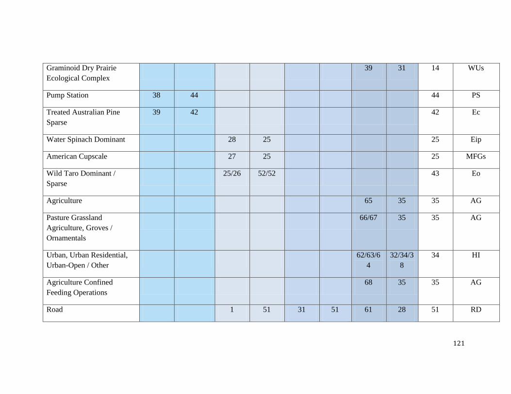
121
Graminoid Dry Prairie
Ecological Complex
39 31 14 WUs
Pump Station 38 44 44 PS
Treated Australian Pine
Sparse
39 42 42 Ec
Water Spinach Dominant 28 25 25 Eip
American Cupscale 27 25 25 MFGs
Wild Taro Dominant /
Sparse
25/26 52/52 43 Eo
Agriculture 65 35 35 AG
Pasture Grassland
Agriculture, Groves /
Ornamentals
66/67 35 35 AG
Urban, Urban Residential,
Urban-Open / Other
62/63/6
4
32/34/3
8
34 HI
Agriculture Confined
Feeding Operations
68 35 35 AG
Road 1 51 31 51 61 28 51 RD
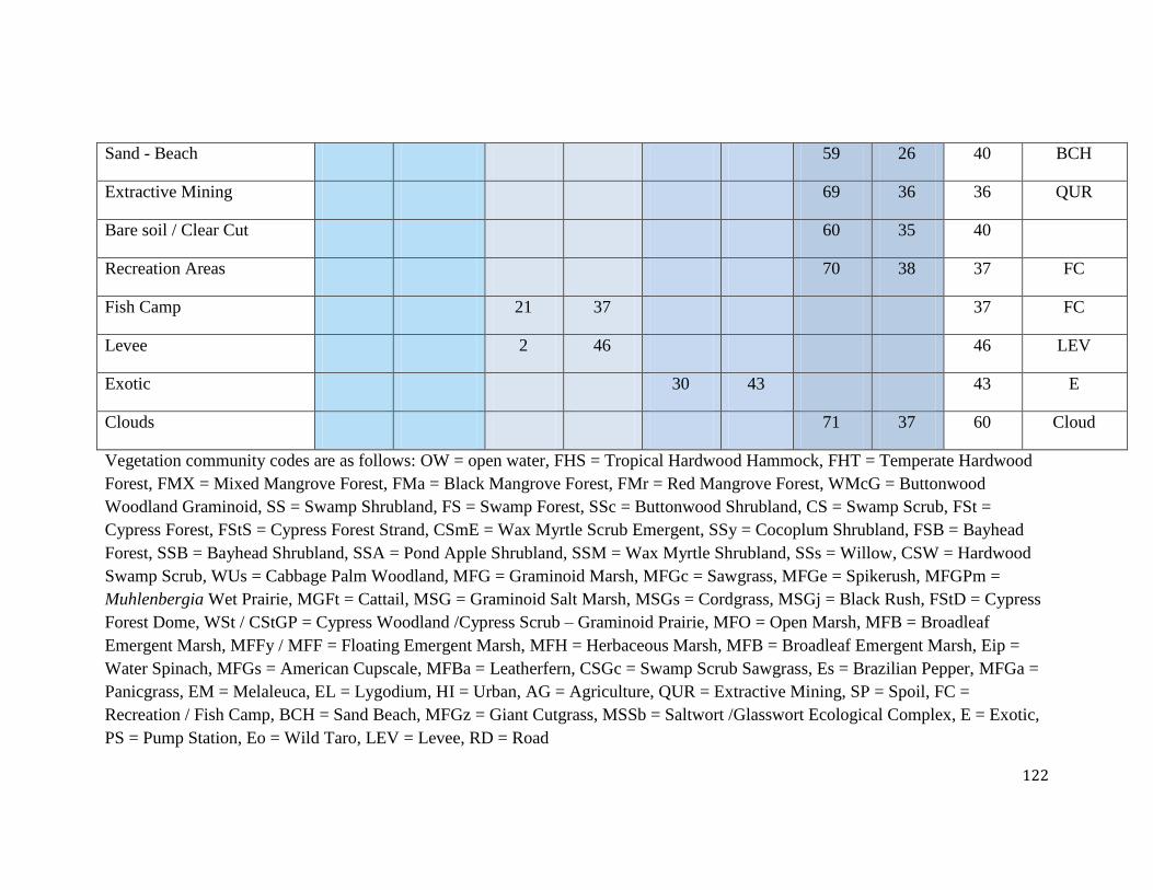
122
Sand - Beach 59 26 40 BCH
Extractive Mining 69 36 36 QUR
Bare soil / Clear Cut 60 35 40
Recreation Areas 70 38 37 FC
Fish Camp 21 37 37 FC
Levee 2 46 46 LEV
Exotic 30 43 43 E
Clouds 71 37 60 Cloud
Vegetation community codes are as follows: OW = open water, FHS = Tropical Hardwood Hammock, FHT = Temperate Hardwood
Forest, FMX = Mixed Mangrove Forest, FMa = Black Mangrove Forest, FMr = Red Mangrove Forest, WMcG = Buttonwood
Woodland Graminoid, SS = Swamp Shrubland, FS = Swamp Forest, SSc = Buttonwood Shrubland, CS = Swamp Scrub, FSt =
Cypress Forest, FStS = Cypress Forest Strand, CSmE = Wax Myrtle Scrub Emergent, SSy = Cocoplum Shrubland, FSB = Bayhead
Forest, SSB = Bayhead Shrubland, SSA = Pond Apple Shrubland, SSM = Wax Myrtle Shrubland, SSs = Willow, CSW = Hardwood
Swamp Scrub, WUs = Cabbage Palm Woodland, MFG = Graminoid Marsh, MFGc = Sawgrass, MFGe = Spikerush, MFGPm =
Muhlenbergia Wet Prairie, MGFt = Cattail, MSG = Graminoid Salt Marsh, MSGs = Cordgrass, MSGj = Black Rush, FStD = Cypress
Forest Dome, WSt / CStGP = Cypress Woodland /Cypress Scrub – Graminoid Prairie, MFO = Open Marsh, MFB = Broadleaf
Emergent Marsh, MFFy / MFF = Floating Emergent Marsh, MFH = Herbaceous Marsh, MFB = Broadleaf Emergent Marsh, Eip =
Water Spinach, MFGs = American Cupscale, MFBa = Leatherfern, CSGc = Swamp Scrub Sawgrass, Es = Brazilian Pepper, MFGa =
Panicgrass, EM = Melaleuca, EL = Lygodium, HI = Urban, AG = Agriculture, QUR = Extractive Mining, SP = Spoil, FC =
Recreation / Fish Camp, BCH = Sand Beach, MFGz = Giant Cutgrass, MSSb = Saltwort /Glasswort Ecological Complex, E = Exotic,
PS = Pump Station, Eo = Wild Taro, LEV = Levee, RD = Road
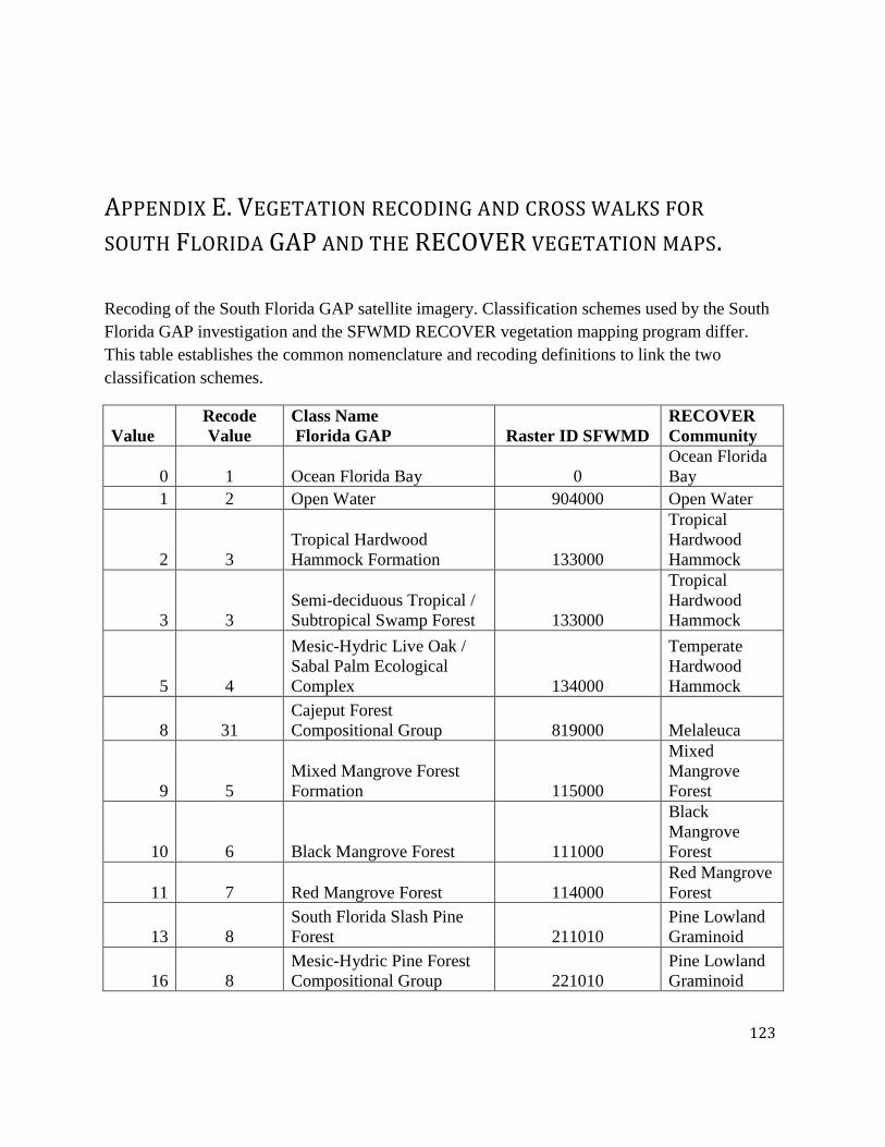
123
APPENDIX E. VEGETATION RECODING AND CROSS WALKS FOR
SOUTH FLORIDA GAP AND THE RECOVER VEGETATION MAPS.
Recoding of the South Florida GAP satellite imagery. Classification schemes used by the South
Florida GAP investigation and the SFWMD RECOVER vegetation mapping program differ.
This table establishes the common nomenclature and recoding definitions to link the two
classification schemes.
Value
Recode
Value
Class Name
Florida GAP Raster ID SFWMD
RECOVER
Community
0 1 Ocean Florida Bay 0
Ocean Florida
Bay
1 2 Open Water 904000 Open Water
2 3
Tropical Hardwood
Hammock Formation 133000
Tropical
Hardwood
Hammock
3 3
Semi-deciduous Tropical /
Subtropical Swamp Forest 133000
Tropical
Hardwood
Hammock
5 4
Mesic-Hydric Live Oak /
Sabal Palm Ecological
Complex 134000
Temperate
Hardwood
Hammock
8 31
Cajeput Forest
Compositional Group 819000 Melaleuca
9 5
Mixed Mangrove Forest
Formation 115000
Mixed
Mangrove
Forest
10 6 Black Mangrove Forest 111000
Black
Mangrove
Forest
11 7 Red Mangrove Forest 114000
Red Mangrove
Forest
13 8
South Florida Slash Pine
Forest 211010
Pine Lowland
Graminoid
16 8
Mesic-Hydric Pine Forest
Compositional Group 221010
Pine Lowland
Graminoid

124
17 9
Swamp Forest Ecological
Complex 120000 Swamp Forests
18 10
Cypress Forest
Compositional Group 127000 Cypress Forest
20 11 Buttonwood Woodland 211000
Buttonwood
Woodland
21 5
Mixed Mangrove
Woodland 115000
Mixed
Mangrove
Forest
22 6 Black Mangrove Woodland 111000
Black
Mangrove
Forest
23 7 Red Mangrove Woodland 114000
Red Mangrove
Forest
25 8
South Florida Slash Pine
Woodland 221010
Pine Lowland
Graminoid
28 12
Flooded Broad-leaved
Evergreen Shrubland
Compositional Group 323000
Bayhead
Forest
29 29
Dry Prairie (Xeric-Mesic)
Ecological Complex 232000
Cabbage Palm
Woodland
31 30 Brazilian Pepper Shrubland 827000
Brazilian
Pepper
32 4
Dwarf Mangrove
Ecological Complex 210000
Mangrove
Woodland
37 13
Saturated - Flooded Cold-
Deciduous and Mixed
Evergreen Cold Deciduous
Shrubland Ecological
Complex 331000
Willow
Shrublands
38 14
Saltwort / Glasswort
Ecological Complex 514000
Succulent Salt
Marsh
39 31
Graminoid Dry Prairie
Ecological Complex 610000
Graminoid
Dune
42 15
Graminoid Emergent Marsh
Compositional Group 522000
Graminoid
Freshwater
Marsh
43 16 Sawgrass Marsh 522100 Sawgrass
44 17 Spikerush Marsh 522200 Spikerush
45 18 Muhlenbergia Grass Marsh 523500
Muhlenbergia
Grass
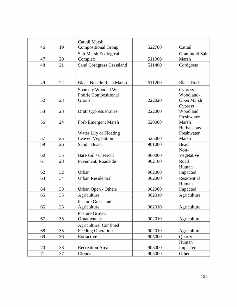
125
46 19
Cattail Marsh
Compositional Group 522700 Cattail
47 20
Salt Marsh Ecological
Complex 511000
Graminoid Salt
Marsh
48 21 Sand Cordgrass Grassland 511400 Cordgrass
49 22 Black Needle Rush Marsh 511200 Black Rush
52 23
Sparsely Wooded Wet
Prairie Compositional
Group 222020
Cypress
Woodland-
Open Marsh
53 23 Draft Cypress Prairie 222000
Cypress
Woodland
56 24 Forb Emergent Marsh 520000
Freshwater
Marsh
57 25
Water Lily or Floating
Leaved Vegetation 525000
Herbaceous
Freshwater
Marsh
59 26 Sand - Beach 901000 Beach
60 35 Bare soil / Clearcut 900000
Non-
Vegetative
61 28 Pavement, Roadside 902100 Road
62 32 Urban 902000
Human
Impacted
63 34 Urban Residential 902000 Residential
64 38 Urban Open / Others 902000
Human
Impacted
65 35 Agriculture 902010 Agriculture
66 35
Pasture Grassland
Agriculture 902010 Agriculture
67 35
Pasture Groves
Ornamentals 902010 Agriculture
68 35
Agricultural Confined
Feeding Operations 902010 Agriculture
69 36 Extractive 905000 Quarry
70 38 Recreation Area 905000
Human
Impacted
71 37 Clouds 905000 Other
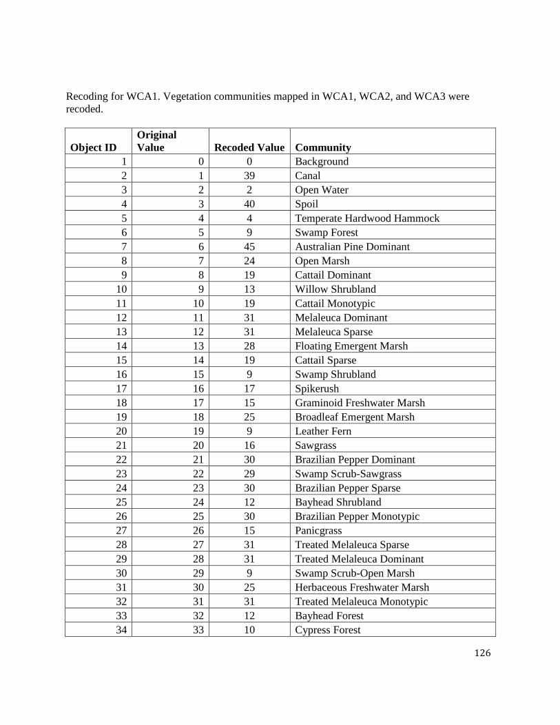
126
Recoding for WCA1. Vegetation communities mapped in WCA1, WCA2, and WCA3 were
recoded.
Object ID
Original
Value Recoded Value Community
1 0 0 Background
2 1 39 Canal
3 2 2 Open Water
4 3 40 Spoil
5 4 4 Temperate Hardwood Hammock
6 5 9 Swamp Forest
7 6 45 Australian Pine Dominant
8 7 24 Open Marsh
9 8 19 Cattail Dominant
10 9 13 Willow Shrubland
11 10 19 Cattail Monotypic
12 11 31 Melaleuca Dominant
13 12 31 Melaleuca Sparse
14 13 28 Floating Emergent Marsh
15 14 19 Cattail Sparse
16 15 9 Swamp Shrubland
17 16 17 Spikerush
18 17 15 Graminoid Freshwater Marsh
19 18 25 Broadleaf Emergent Marsh
20 19 9 Leather Fern
21 20 16 Sawgrass
22 21 30 Brazilian Pepper Dominant
23 22 29 Swamp Scrub-Sawgrass
24 23 30 Brazilian Pepper Sparse
25 24 12 Bayhead Shrubland
26 25 30 Brazilian Pepper Monotypic
27 26 15 Panicgrass
28 27 31 Treated Melaleuca Sparse
29 28 31 Treated Melaleuca Dominant
30 29 9 Swamp Scrub-Open Marsh
31 30 25 Herbaceous Freshwater Marsh
32 31 31 Treated Melaleuca Monotypic
33 32 12 Bayhead Forest
34 33 10 Cypress Forest
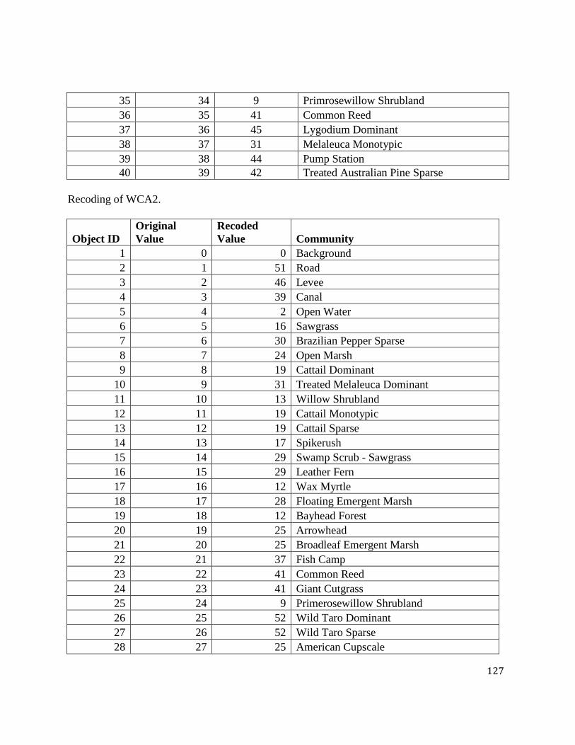
127
35 34 9 Primrosewillow Shrubland
36 35 41 Common Reed
37 36 45 Lygodium Dominant
38 37 31 Melaleuca Monotypic
39 38 44 Pump Station
40 39 42 Treated Australian Pine Sparse
Recoding of WCA2.
Object ID
Original
Value
Recoded
Value Community
1 0 0 Background
2 1 51 Road
3 2 46 Levee
4 3 39 Canal
5 4 2 Open Water
6 5 16 Sawgrass
7 6 30 Brazilian Pepper Sparse
8 7 24 Open Marsh
9 8 19 Cattail Dominant
10 9 31 Treated Melaleuca Dominant
11 10 13 Willow Shrubland
12 11 19 Cattail Monotypic
13 12 19 Cattail Sparse
14 13 17 Spikerush
15 14 29 Swamp Scrub - Sawgrass
16 15 29 Leather Fern
17 16 12 Wax Myrtle
18 17 28 Floating Emergent Marsh
19 18 12 Bayhead Forest
20 19 25 Arrowhead
21 20 25 Broadleaf Emergent Marsh
22 21 37 Fish Camp
23 22 41 Common Reed
24 23 41 Giant Cutgrass
25 24 9 Primerosewillow Shrubland
26 25 52 Wild Taro Dominant
27 26 52 Wild Taro Sparse
28 27 25 American Cupscale

128
29 28 25 Water Spinach Dominant
30 29 12 Bayhead Shrubland

129
Recoding of WCA3.
Object ID Original Value Recoded Value Community
1 1 40 Spoil
2 2 9 Swamp Shrubland
3 3 24 Broadleaf Emergent Marsh
4 4 19 Cattail
5 5 16 Sawgrass
6 6 24 Open Marsh
7 7 28 Floating Emergent Marsh
8 8 41 Common Reed
9 9 13 Willow Shrubland
10 10 2 Open Water
11 11 15 Graminoid Freshwater Marsh
12 12 39 Canal
13 13 29 Leather Fern
14 14 9 Pond Apple Shrubland
15 15 10 Cypress Forest
16 16 9 Swamp Forest
17 17 30 Brazilian Pepper
18 18 10 Cypress Scrub
19 19 10 Cypress Forest-Dome
20 21 9 Buttonbush Shrubland
21 22 31 Melaleuca
22 23 25 Herbaceous Freshwater Marsh
23 24 17 Spikerush
24 25 9 Cocoplum Shrubland
25 26 9 Wax Myrtle Shrubland
26 27 9 Primerosewillow Shrubland
27 28 15 Panicgrass
28 30 43 Exotics
29 31 51 Road