

UNIVERSIDAD CARLOS III DE MADRID
Ph.D program in Electrical Engineering, Electronics and Automation
The review committee approves the doctoral thesis titled “CONTINUOUS GOAL-
DIRECTED ACTIONS: ADVANCES IN ROBOT LEARNING” written by Santiago
Morante Cendrero and directed by Dr. Juan Carlos Gonzalez Vıctores and Dr. Carlos
Balaguer Bernaldo de Quiros.
Signature of the Review Committee:
President:
Secretary:
Member:
Grade:
Date:


“It took time, but I learned the patterns. At first, the sheer complexity
made the task seem impossible. But then I felt the satisfaction of
breaking the code”
Daniel H. Wilson, Robogenesis


vii
Acknowledgments
First, I would like to thank Juan Carlos Gonzalez Victores. He has been more than
an advisor. He has been my friend during the journey, helped me with the “software
stuff”, amazed me with his programming skills, and wrote (and reviewed) with me
every paper we published. Thank you Johnny!
I also would like to express my gratitude to my advisor Carlos Balaguer for sup-
porting me and for letting me deviate from my research topic more often than not. I
can’t thank enough to my Robotics Lab colleagues, specially Alvaro Villoslada, Roberto
Montero, and Jorge Munoz, for being so easy going and kind.
Finally, I will like to thank my parents for their support, and Lourdes, because she
is my pillar of strength.

viii
ix
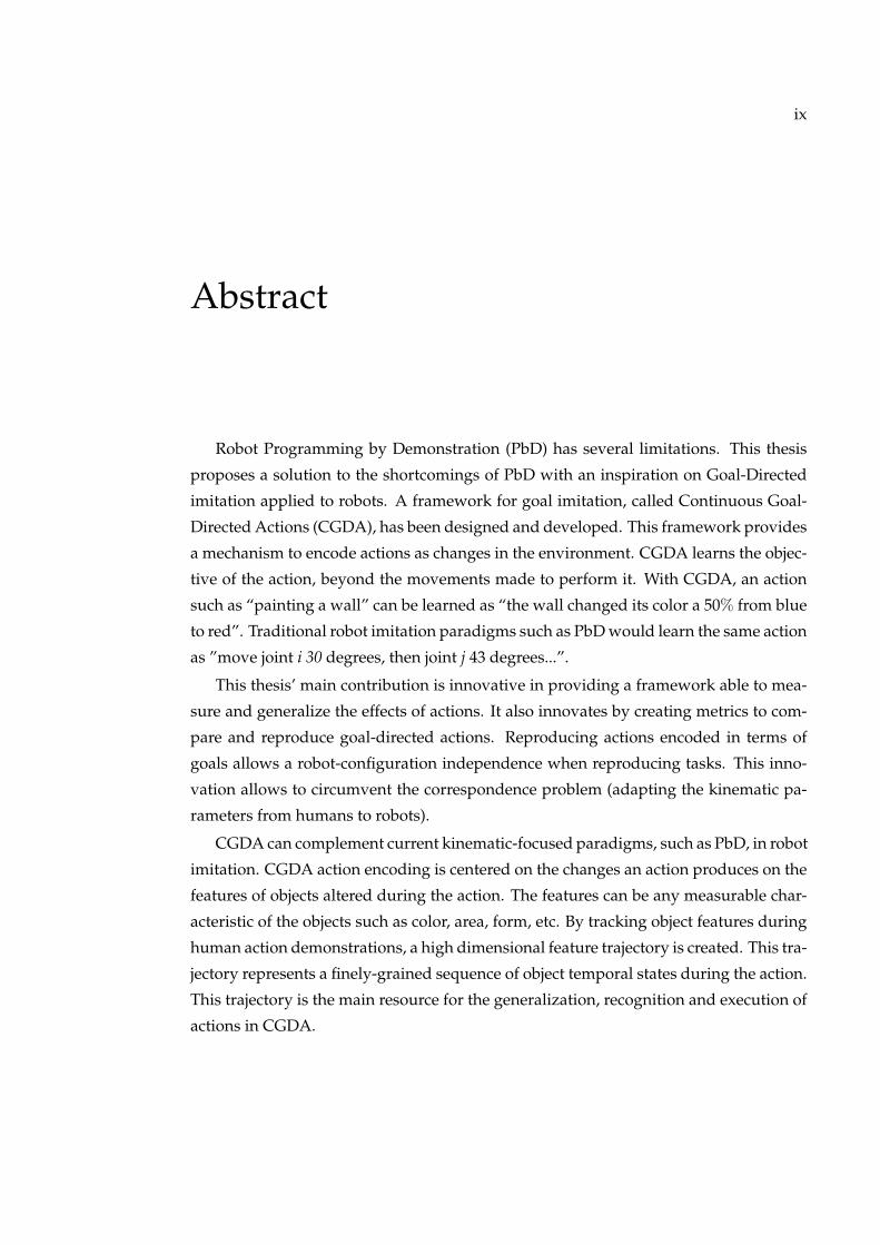
Abstract
Robot Programming by Demonstration (PbD) has several limitations. This thesis
proposes a solution to the shortcomings of PbD with an inspiration on Goal-Directed
imitation applied to robots. A framework for goal imitation, called Continuous Goal-
Directed Actions (CGDA), has been designed and developed. This framework provides
a mechanism to encode actions as changes in the environment. CGDA learns the objec-
tive of the action, beyond the movements made to perform it. With CGDA, an action
such as “painting a wall” can be learned as “the wall changed its color a 50% from blue
to red”. Traditional robot imitation paradigms such as PbD would learn the same action
as ”move joint i 30 degrees, then joint j 43 degrees...”.
This thesis’ main contribution is innovative in providing a framework able to mea-
sure and generalize the effects of actions. It also innovates by creating metrics to com-
pare and reproduce goal-directed actions. Reproducing actions encoded in terms of
goals allows a robot-configuration independence when reproducing tasks. This inno-
vation allows to circumvent the correspondence problem (adapting the kinematic pa-
rameters from humans to robots).
CGDA can complement current kinematic-focused paradigms, such as PbD, in robot
imitation. CGDA action encoding is centered on the changes an action produces on the
features of objects altered during the action. The features can be any measurable char-
acteristic of the objects such as color, area, form, etc. By tracking object features during
human action demonstrations, a high dimensional feature trajectory is created. This tra-
jectory represents a finely-grained sequence of object temporal states during the action.
This trajectory is the main resource for the generalization, recognition and execution of
actions in CGDA.

x
Around this presented framework, several components have been added to fa-
cilitate and improve the imitation. Naıve implementations of robot learning frame-
works usually assume that all the data from the user demonstrations has been correctly
sensed and is relevant to the task. This assumption proves wrong in most human-
demonstrated learning scenarios. This thesis presents an automatic demonstration and
feature selection process to solve this issue. This machine learning pipeline is called
Dissimilarity Mapping Filtering (DMF). DMF can filter both irrelevant demonstrations
and irrelevant features.
Once an action is generalized from a series of correct human demonstrations, the
robot must be provided a method to reproduce this action. Robot joint trajectories
are computed in simulation using evolutionary computation through diverse proposed
strategies. This computation can be improved by using human-robot interaction. Specif-
ically, a system for robot discovery of motor primitives from random human-guided
movements has been developed. These Guided Motor Primitives (GMP) are combined
to reproduce goal-directed actions.
To test all these developments, experiments have been performed using a humanoid
robot in a simulated environment, and the real full-sized humanoid robot TEO. A brief
analysis about the cyber safety of current robots is additionally presented in the final
appendices of this thesis.
Keywords: robot learning, humanoid robots, goal-directed actions, motor primitives,
feature selection, demonstration selection, cryptobotics.
xi
Resumen
Robot Programming by demonstration (PbD) tiene varias limitaciones. Esta tesis
propone una solucion a las carencias de PbD, inspirandose en la imitacion dirigida a
objetivos en robots. Se ha disenado y desarrollado un marco de trabajo para la imitacion
de objetivos llamado Continuous Goal-Directed Actions (CGDA). Este marco de trabajo
proporciona un mecanismo para codificar acciones como cambios en el entorno. CGDA
aprende los objetivos de la accion, mas alla de los movimientos hechos para realizarla.
Con CGDA, una accion como “pintar una pared”se puede aprender como “la pared
cambio su color un 50 % de azul a rojo”. Paradigmas tradicionales de imitacion robotica
como PbD aprenderıan la misma accion como “mueve la articulacion i 30 grados, luego
la articulacion j 43 grados...”.
La contribucion principal de esta tesis es innovadora en proporcionar un marco de
trabajo capaz de medir y generalizar los efectos de las acciones. Tambien innova al crear
metricas para comparar y reproducir acciones dirigidas a objetivos. Reproducir accio-
nes codificadas como objetvos permite independizarse de la configuracion del robot
cuando se reproducen las acciones. Esta innovacion permite sortear el problema de la
correspondencia (adaptar los parametros cinematicos de los humanos a los robots).
CGDA puede complementar paradigmas centrados en la cinematica, como PbD, en
la imitacion robotica. CGDA codifica las acciones centrandose en los cambios produ-
cidos por la accion en las caracterısticas de los objetos afectados por esta. Las carac-
terısticas pueden ser cualquier rasgo medible de los objetos, como color, area, forma,
etc. Midiendo las caracterısticas de los objetos durante las demostraciones humanas se
crea una trayectoria de alta dimensionalidad. Esta trayectoria representa una detallada
secuencia de los estados temporales del objeto durante la accion. Esta trayectoria es el
xii
recurso principal para la generalizacion, el reconocimiento y la ejecucion de acciones
en CGDA.
Alrededor del marco de trabajo presentado, se han anadido algunos componen-
tes para facilitar y mejorar la imitacion. Las implementaciones simples en aprendizaje
robotico normalmente asumen que todos los datos provenientes de las demostraciones
del usuario han sido correctamente medidos y son relevantes para la tarea. Esta supo-
sicion se demuestra falsa en la mayorıa de escenarios de aprendizaje por demostracion
humana. Esta tesis presenta un proceso de seleccion automatico de demostraciones y
caracteristicas para resolver este problema. Este proceso de aprendizaje automatico se
llama Dissimilarity Mapping Filtering (DMF). DMF puede filtrar tanto demostraciones
irrelevantes, como caracterısticas innecesarias.
Una vez que una accion se ha generalizado a partir de una serie de demostracio-
nes humanas, es necesario proveer al robot de un metodo para reproducir la accion.
Las trayectorias articulares del robot se computan en simulacion usando computacion
evolutiva. Esta computacion se puede mejorar usando interaccion humano-robot. Es-
pecificamente, se ha desarrollado un sistema para el descubrimiento de primitivas de
movimiento del robot a partir de movimientos aleatorios, guiados por el humano. Es-
tas primitivas, llamadas Guided Motor Primitives (GMP), se conbinan para reproducir
acciones centradas en objetivos.
Para probar estos desarrollos, los experimentos se han llevado a cabo usando un ro-
bot humanoide en un entorno simulado, y el robot humanoide real TEO. En los apendi-
ces finales de esta tesis se presenta un breve analisis de la ciberseguridad de los robots
actuales .
Palabras clave: aprendizaje robotico, robots humanoides, acciones centradas en obje-
tivos, primitivas de movimiento, seleccion de caracterısticas, seleccion de demostracio-
nes, cryptobotics.
xiii
Contents
Acknowledgments vii
Abstract ix
Resumen xi
Contents xiii
Index of Figures xvii
Index of Tables xxiii
1 Introduction 1
1.1 New Mechanisms for Programming Robots . . . . . . . . . . . . . . . . . 1
1.2 Overview and Definitions . . . . . . . . . . . . . . . . . . . . . . . . . . . 2
1.3 Motivation . . . . . . . . . . . . . . . . . . . . . . . . . . . . . . . . . . . . 4
1.4 Main Objectives . . . . . . . . . . . . . . . . . . . . . . . . . . . . . . . . . 6
1.5 Scientific Contributions . . . . . . . . . . . . . . . . . . . . . . . . . . . . . 6
1.6 Document Structure . . . . . . . . . . . . . . . . . . . . . . . . . . . . . . 7
2 Background 9
2.1 Programming by Demonstration . . . . . . . . . . . . . . . . . . . . . . . 9
2.2 Goal-Directed Actions . . . . . . . . . . . . . . . . . . . . . . . . . . . . . 11
2.3 Demonstration and Feature Selection . . . . . . . . . . . . . . . . . . . . . 15
2.4 Motor Primitives . . . . . . . . . . . . . . . . . . . . . . . . . . . . . . . . 18
xiv CONTENTS
2.5 Physical Interaction with Robots . . . . . . . . . . . . . . . . . . . . . . . 20
2.6 Chapter Summary . . . . . . . . . . . . . . . . . . . . . . . . . . . . . . . . 23
3 Continuous Goal-Directed Actions 25
3.1 Differences between CGDA and PbD . . . . . . . . . . . . . . . . . . . . . 26
3.2 Selecting Relevant Demonstrations and Features . . . . . . . . . . . . . . 29
3.3 Basic CGDA Framework . . . . . . . . . . . . . . . . . . . . . . . . . . . . 29
3.4 Generating a Library of Motor Primitives . . . . . . . . . . . . . . . . . . 30
3.5 Compensating Friction and Gravity . . . . . . . . . . . . . . . . . . . . . 31
4 Demonstration and Feature Selection 33
4.1 Dissimilarity Mapping Filtering . . . . . . . . . . . . . . . . . . . . . . . . 35
4.2 Demonstration Selector . . . . . . . . . . . . . . . . . . . . . . . . . . . . . 35
4.2.1 Preprocessing . . . . . . . . . . . . . . . . . . . . . . . . . . . . . . 37
4.2.2 Dissimilarity . . . . . . . . . . . . . . . . . . . . . . . . . . . . . . . 38
4.2.3 Mapping . . . . . . . . . . . . . . . . . . . . . . . . . . . . . . . . . 41
4.2.4 Filtering . . . . . . . . . . . . . . . . . . . . . . . . . . . . . . . . . 41
4.3 Feature Selector . . . . . . . . . . . . . . . . . . . . . . . . . . . . . . . . . 42
4.3.1 Preprocessing . . . . . . . . . . . . . . . . . . . . . . . . . . . . . . 43
4.3.2 Dissimilarity . . . . . . . . . . . . . . . . . . . . . . . . . . . . . . . 43
4.3.3 Mapping . . . . . . . . . . . . . . . . . . . . . . . . . . . . . . . . . 44
4.3.4 Filtering . . . . . . . . . . . . . . . . . . . . . . . . . . . . . . . . . 45
5 Generalization and Recognition 47
5.1 Generalization . . . . . . . . . . . . . . . . . . . . . . . . . . . . . . . . . . 47
5.1.1 Time Rescaling . . . . . . . . . . . . . . . . . . . . . . . . . . . . . 48
5.1.2 Average in Temporal Intervals . . . . . . . . . . . . . . . . . . . . 48
5.1.3 Radial Basis Function Interpolation . . . . . . . . . . . . . . . . . 48
5.2 Recognition . . . . . . . . . . . . . . . . . . . . . . . . . . . . . . . . . . . 51
5.2.1 Dynamic Time Warping . . . . . . . . . . . . . . . . . . . . . . . . 51
5.2.2 Euclidean Distance . . . . . . . . . . . . . . . . . . . . . . . . . . . 52
6 Execution 55
6.1 Simulation using Evolutionary Strategies . . . . . . . . . . . . . . . . . . 56
6.1.1 Full Trajectory Evolution . . . . . . . . . . . . . . . . . . . . . . . 57
CONTENTS xv
6.1.2 Individual Evolution . . . . . . . . . . . . . . . . . . . . . . . . . . 57
6.1.3 Incrementally Evolved Trajectories . . . . . . . . . . . . . . . . . . 57
6.2 Guided Motor Primitives . . . . . . . . . . . . . . . . . . . . . . . . . . . . 58
6.2.1 Sequential Incremental Combinatorial Search . . . . . . . . . . . . 61
6.2.2 Force-Sensorless Friction and Gravity Compensation . . . . . . . 65
7 Experiments 73
7.1 Demonstration and Feature Selection . . . . . . . . . . . . . . . . . . . . . 74
7.1.1 Demonstration Selector . . . . . . . . . . . . . . . . . . . . . . . . 75
7.1.2 Feature Selector . . . . . . . . . . . . . . . . . . . . . . . . . . . . . 78
7.2 CGDA Recognition . . . . . . . . . . . . . . . . . . . . . . . . . . . . . . . 80
7.2.1 Object Feature Trajectory Recognition . . . . . . . . . . . . . . . . 80
7.2.2 Cartesian Space Trajectory Recognition . . . . . . . . . . . . . . . 82
7.3 CGDA Execution by Evolutionary Computation . . . . . . . . . . . . . . 82
7.3.1 Executing a Spatial Task: Cleaning . . . . . . . . . . . . . . . . . . 84
7.3.2 Executing a Non-Spatial Task: Painting . . . . . . . . . . . . . . . 86
7.4 Guided Motor Primitives . . . . . . . . . . . . . . . . . . . . . . . . . . . . 91
7.4.1 Executing a Spatial Task: Cleaning . . . . . . . . . . . . . . . . . . 91
7.4.2 Executing a Non-Spatial Task: Painting . . . . . . . . . . . . . . . 92
7.5 Friction and Gravity Compensation . . . . . . . . . . . . . . . . . . . . . 94
7.5.1 Computation . . . . . . . . . . . . . . . . . . . . . . . . . . . . . . 95
7.5.2 Evaluation . . . . . . . . . . . . . . . . . . . . . . . . . . . . . . . . 97
8 Discussion and Conclussions 99
8.1 Normalization on Demonstration and Feature Selection . . . . . . . . . . 99
8.2 Limitations of CGDA . . . . . . . . . . . . . . . . . . . . . . . . . . . . . . 100
8.3 The Benefits of Human-Robot Interaction . . . . . . . . . . . . . . . . . . 101
8.4 A More Accurate Compensation . . . . . . . . . . . . . . . . . . . . . . . 101
8.5 Conclusions . . . . . . . . . . . . . . . . . . . . . . . . . . . . . . . . . . . 102
8.6 Future Lines of Research . . . . . . . . . . . . . . . . . . . . . . . . . . . . 103
A Opinion: Cryptobotics 107
A.1 Stating The Problem . . . . . . . . . . . . . . . . . . . . . . . . . . . . . . 107
A.2 Current State of Security in Mainstream Robotic Software . . . . . . . . . 110

xvi CONTENTS
A.3 Guidelines and Security Checks . . . . . . . . . . . . . . . . . . . . . . . . 112
A.4 Discussion . . . . . . . . . . . . . . . . . . . . . . . . . . . . . . . . . . . . 114
B TEO, The Humanoid Robot 115
Bibliography 125
xvii
Index of Figures
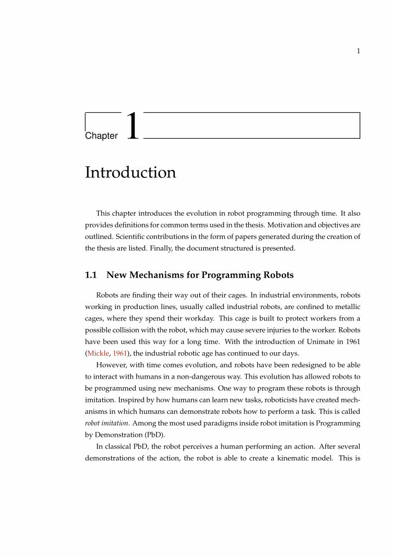
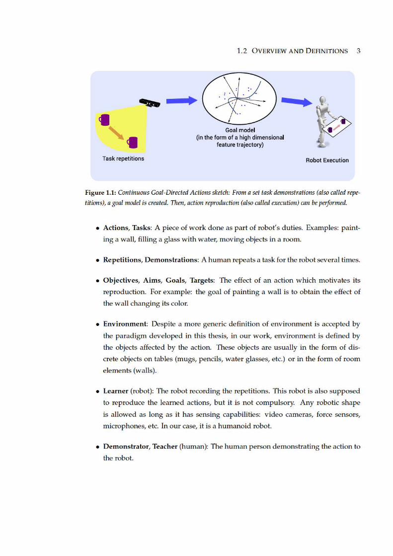
1.1 Continuous Goal-Directed Actions sketch: From a set task demonstra-
tions (also called repetitions), a goal model is created. Then, action re-
production (also called execution) can be performed. . . . . . . . . . . . 3
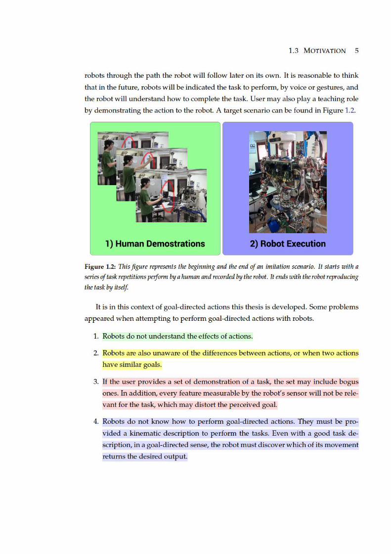
1.2 This figure represents the beginning and the end of an imitation sce-
nario. It starts with a series of task repetitions perform by a human and
recorded by the robot. It ends with the robot reproducing the task by itself. 5
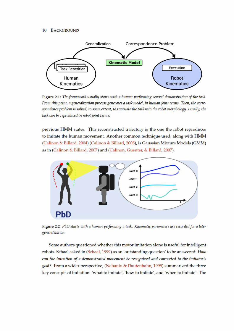
2.1 The framework usually starts with a human performing several demon-
stration of the task. From this point, a generalization process generates a
task model, in human joint terms. Then, the correspondence problem is
solved, to some extent, to translate the task into the robot morphology.
Finally, the task can be reproduced in robot joint terms. . . . . . . . . . . 10
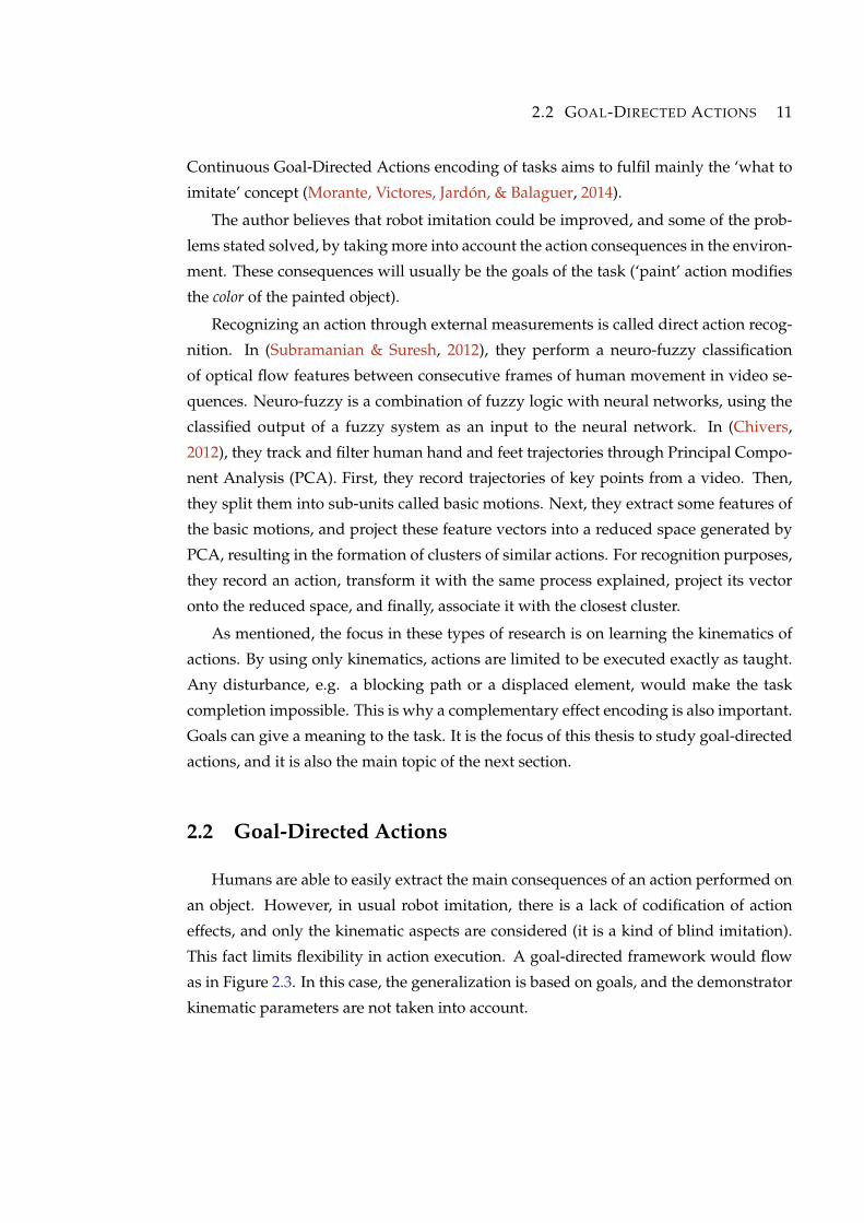
2.2 PbD starts with a human performing a task. Kinematic parameters are
recorded for a later generalization. . . . . . . . . . . . . . . . . . . . . . . 10
2.3 The goal-directed framework usually starts with a human performing
several demonstration of the task. From this point, a generalization pro-
cess generates a goal model, in terms of the consequences of the action in
the environment. Then, the execution problem is solved to translate the
goal model into a kinematic model. Finally, the task can be reproduced
in robot joint terms. . . . . . . . . . . . . . . . . . . . . . . . . . . . . . . . 12
xviii INDEX OF FIGURES
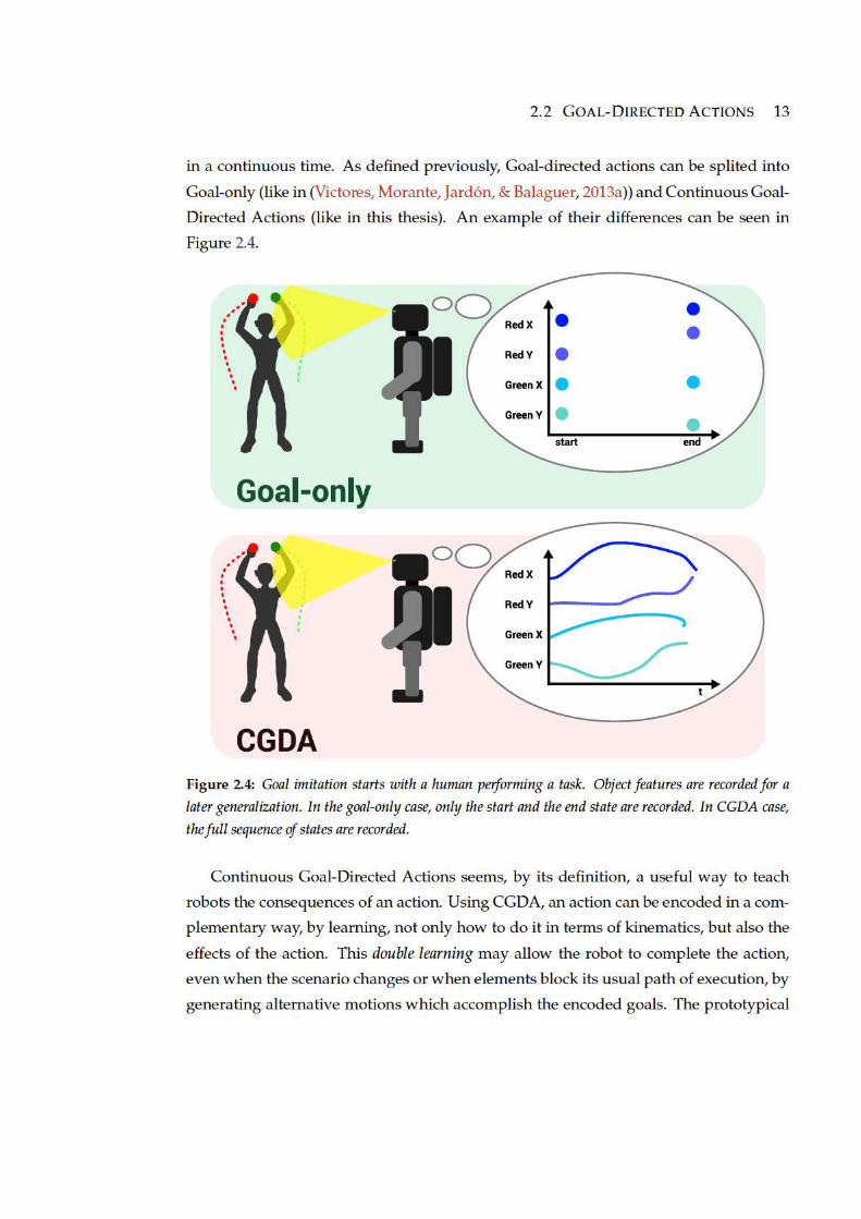
2.4 Goal imitation starts with a human performing a task. Object features
are recorded for a later generalization. In the goal-only case, only the
start and the end state are recorded. In CGDA case, the full sequence of
states are recorded. . . . . . . . . . . . . . . . . . . . . . . . . . . . . . . . 13
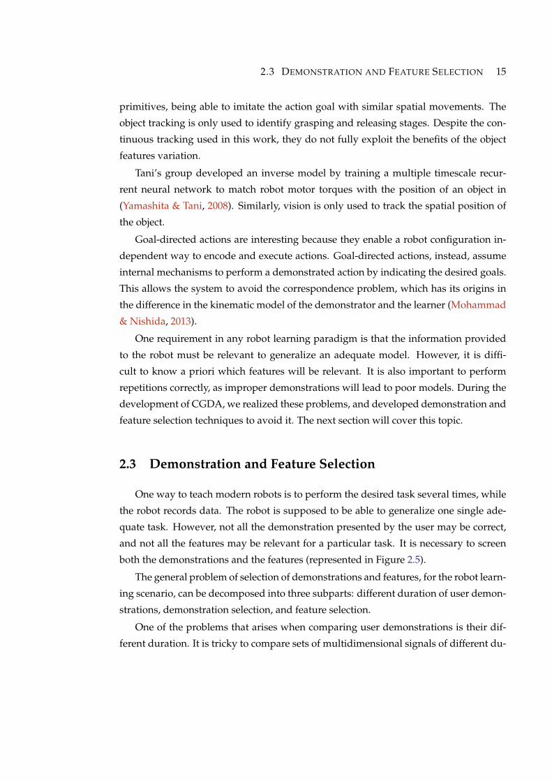
2.5 In the upper block, demonstration selection is carried out. From the set
of complete demonstrations (each one represented as an axis frame with
blue lines), the most different are discarded. In the lower block, feature
selection is carried out. From the set of features, those feature which are
not similar across demonstration are removed. . . . . . . . . . . . . . . . 16
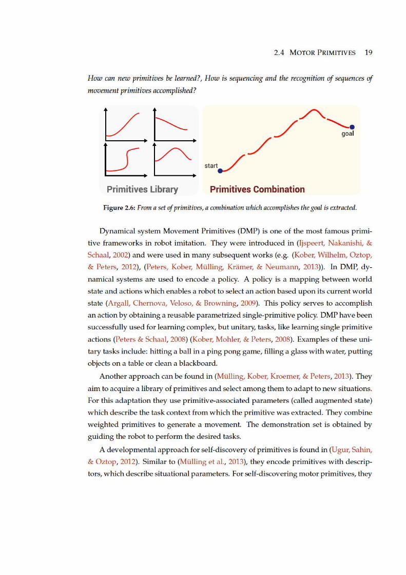
2.6 From a set of primitives, a combination which accomplishes the goal is
extracted. . . . . . . . . . . . . . . . . . . . . . . . . . . . . . . . . . . . . . 19
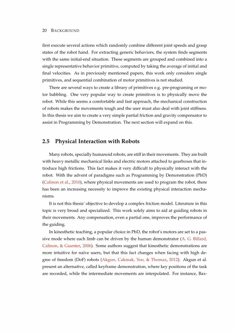
2.7 Without compensation, robots are very stiff to be moved. With compen-
sation, even a partial one, robots can be guided easily. . . . . . . . . . . . 21
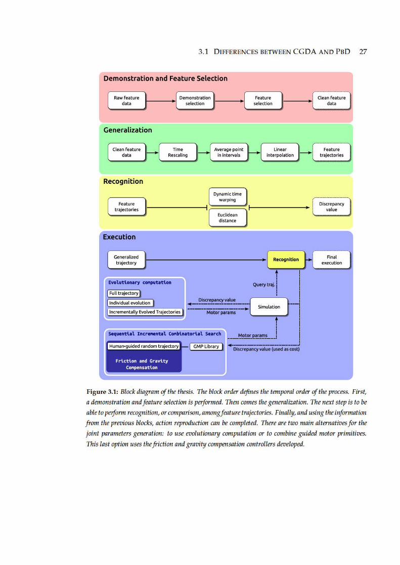
3.1 Block diagram of the thesis. The block order defines the temporal order
of the process. First, a demonstration and feature selection is performed.
Then comes the generalization. The next step is to be able to perform
recognition, or comparison, among feature trajectories. Finally, and us-
ing the information from the previous blocks, action reproduction can be
completed. There are two main alternatives for the joint parameters gen-
eration: to use evolutionary computation or to combine guided motor
primitives. This last option uses the friction and gravity compensation
controllers developed. . . . . . . . . . . . . . . . . . . . . . . . . . . . . . 27
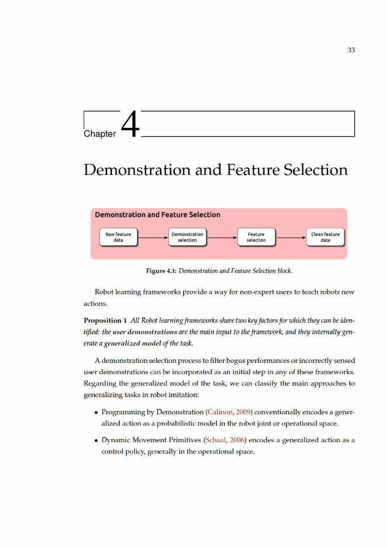
4.1 Demonstration and Feature Selection block. . . . . . . . . . . . . . . . . . 33
4.2 Imagine we want to screen the most irrelevant of the three signals. First,
we extract a measure of dissimilarities among them. These dissimilar-
ities can be represented as nodes’ distances in a graph. Then, we map
these distances from a matrix to a single dimension e.g. by summing the
columns. In the last step, we can represent values in a bar plot. To further
increase their differences, a transformation, e.g. z-score, is applied. This
transformation allows to better distinguish the irrelevant signal, which
can now be filtered with a threshold (represented by a dotted red line). . 36
4.3 Humanoid robotics learning scenario: block-moving task. . . . . . . . . 36
INDEX OF FIGURES xix
4.4 Different preprocessing methods for reducing multidimensional infor-
mation. . . . . . . . . . . . . . . . . . . . . . . . . . . . . . . . . . . . . . . 39
4.5 Example of accumulated cost matrix for two sequences. On the left side,
the interpolated sequences are shown. The right side depicts the Dy-
namic Time Warping computation. White cells represent high cost, while
dark cells are low cost ones. The red line is the lowest cost path. . . . . . 40
4.6 For each feature space, a distance matrix is calculated. Each color line
(red, blue and green) is the same feature but extracted from a different
demonstration. When represented in the same space, these features tra-
jectories will show some kind of similarity if they are relevant, or will be
different if they are not. . . . . . . . . . . . . . . . . . . . . . . . . . . . . . 44
5.1 Generalization block. . . . . . . . . . . . . . . . . . . . . . . . . . . . . . . 47
5.2 Plot representing a three feature trajectory. Black lines are training action
repetitions. The blue dots are the averaged points. . . . . . . . . . . . . . 49
5.3 Plot representing a three feature trajectory. Black lines are training action
repetitions. The blue line is the generalization of all the repetitions. . . . 50
5.4 Recognition block. . . . . . . . . . . . . . . . . . . . . . . . . . . . . . . . 51
5.5 Two alternatives are presented to be used as distance measures. . . . . . 53
6.1 Execution block. . . . . . . . . . . . . . . . . . . . . . . . . . . . . . . . . . 55
6.2 Evolutionary block. . . . . . . . . . . . . . . . . . . . . . . . . . . . . . . . 56
6.3 Guided Motor Primitives block. . . . . . . . . . . . . . . . . . . . . . . . . 59
6.4 Human guiding the robot in a random spatial trajectory. The red lines
represent an example of the joints’ spatial trajectories during the guiding. 59
6.5 This random joint trajectory involves 3 joints of the robot arm. It is gener-
ated when the human performs some random movements with the robot
arm. . . . . . . . . . . . . . . . . . . . . . . . . . . . . . . . . . . . . . . . . 60
6.6 An example of comparison between two random segments extracted
from the previously shown joint trajectory. Both segments have a du-
ration of τ = 0.5 s and the blue lines represent the distances between
pairs of points. . . . . . . . . . . . . . . . . . . . . . . . . . . . . . . . . . . 61
6.7 Several examples of guided motor primitives in the joint space. They
were extracted from the joint trajectory shown in Figure 6.5. . . . . . . . 62
xx INDEX OF FIGURES
6.8 SICS example for a two-point feature trajectory. For the first point, the
nodes are expanded and a breadth-first search is performed until the cost
of one of the nodes is lower than a threshold ε. If this occurs, the path
to the node is stored and the process continues for the next point. If not,
the tree is expanded one level of depth, and the search repeats. . . . . . . 64
6.9 Friction and Gravity Compensation block. . . . . . . . . . . . . . . . . . . 65
6.10 Block scheme of friction and gravity compensation. In this type of con-
trol, there is no external reference, the robotic system is moved by the
external perturbations caused by the user. . . . . . . . . . . . . . . . . . . 66
6.11 This friction model includes Coulomb friction and viscous friction. The
variables α and β represent the parameters of the linear model assumed. 69
7.1 User demonstrations from TEO’s perspective; red segmentation on the
bottom left, and green segmentation on the bottom right. . . . . . . . . . 74
7.2 Red object centroid coordinates throughout time. . . . . . . . . . . . . . . 76
7.3 Green object centroid coordinates throughout time. . . . . . . . . . . . . 77
7.4 Demonstration selection’s z-scores without data normalization, prepro-
cessed by summing columns, setting the threshold to α = 0.5. . . . . . . 77
7.5 Demonstration selection’s z-scores without data normalization, prepro-
cessed by summing rows, setting the threshold to α = 0.5. . . . . . . . . 78
7.6 Feature selection’s z-scores without data normalization, setting the thresh-
old to α = 0.5. . . . . . . . . . . . . . . . . . . . . . . . . . . . . . . . . . . 79
7.7 Graphical representation of the actions performed in this experiment. . . 80
7.8 The picture shows the experimental scenario with the robot, the object
(green) and the Kinect camera. The bottom left square is the Kinect depth
map and the bottom right square shows the color segmentation of the
object. . . . . . . . . . . . . . . . . . . . . . . . . . . . . . . . . . . . . . . . 83
7.9 Fitness value through evolution. The red point is the minimum value
achieved by evolution. . . . . . . . . . . . . . . . . . . . . . . . . . . . . . 85
7.10 Unidimensional temporal plots of generalized reference (blue), and the
object feature space trajectory from executing the EC winner joint posi-
tion trajectory (red). The Z dimension gives the worst results. The system
was not able to reduce the error in this dimension. . . . . . . . . . . . . . 86
INDEX OF FIGURES xxi
7.11 Unidimensional temporal plots of the generalized action, and the trajec-
tory obtained by executing the EC winner joint parameters. The trajecto-
ries are quite similar for all cases. In the case of Z dimension, which may
look like a less well-defined result, it is important to check its units. In
none of the points the error is bigger than 20 mm. . . . . . . . . . . . . . 87
7.12 Plot representing a three feature trajectory. Black lines are training action
repetitions. The blue line is the generalization extracted from all the repe-
titions. The red line is the evolved trajectory. Note that none of the points
of the evolved trajectory has an error bigger than 20 mm with respect to
its reference (the generalized). . . . . . . . . . . . . . . . . . . . . . . . . 88
7.13 Action execution for a CLEAN command. Despite the trajectory is purely
spatial, the objective of the evolution and the execution is to perform a
feature trajectory obtained from the object tracker. . . . . . . . . . . . . . 88
7.14 In this chart the time taken to compute each point is shown. Except for
one final point (where the valid space is already very restricted) the time
of computation increases linearly. . . . . . . . . . . . . . . . . . . . . . . . 89
7.15 Unidimensional temporal plot of the generalized action, and the trajec-
tory obtained by executing the EC winner joint parameters. As seen for
a linear painting task (one wall square is painted in each step), the per-
formance is very accurate. . . . . . . . . . . . . . . . . . . . . . . . . . . . 90
7.16 Action execution for a PAINT command. Each square changes its color
when the hand gets closer than a specific distance. . . . . . . . . . . . . . 90
7.17 Cleaning: Plot superposing the generalized feature trajectory (blue) and
several feature trajectories resulting from executing the sequence of prim-
itives selected by SICS. Results are dependent on the number of primi-
tives available to choose from (given by the threshold of similarity ξ) and
the maximum tree depth d. The primitives used belong to the same set
of segments, but in function of ξ, the most diverse are selected. . . . . . . 92
7.18 Painting: Plot superposing the generalized feature trajectory (blue) and
several feature trajectories resulting from executing the sequence of prim-
itives selected by SICS. Results are dependent on the number of primi-
tives available to choose from (given by the threshold ξ). Remember the
plot is not representing joint or spatial trajectories, but feature ones. . . . 93
xxii INDEX OF FIGURES
7.19 Several screenshots taken during the painting experiment. Motor se-
quence obtained from combining primitives using SICS. . . . . . . . . . 94
7.20 Velocity vs. time curves, with constant torques applied in each curve.
There is a proportional linear dependence between current in the motor
and torque applied. . . . . . . . . . . . . . . . . . . . . . . . . . . . . . . . 96
7.21 Stabilization velocity vs. the torque applied. The Coulomb friction (blue)
and the viscous friction (red) can be seen. The same procedure is applied
to negative velocities. . . . . . . . . . . . . . . . . . . . . . . . . . . . . . . 96
7.22 Velocity profiles for several initial ‘pushes’ with the Zero-Friction Zero-
Gravity controller (ZFZG). . . . . . . . . . . . . . . . . . . . . . . . . . . . 98
7.23 Sequence of the movement of the robot arm using a Zero-Friction Zero-
Gravity controller. When the user pushes the arm, it moves freely in the
direction of the applied force. . . . . . . . . . . . . . . . . . . . . . . . . . 98
B.1 Axes and directions of rotation of humanoid robot TEO. . . . . . . . . . 116
B.2 Denavit-Hartenberg directions of humanoid robot TEO. . . . . . . . . . . 117
B.3 Denavit-Hartenberg parameters of humanoid robot TEO. . . . . . . . . . 118
B.4 CAN (Controller Area Network) identification number of the joints of
humanoid robot TEO. . . . . . . . . . . . . . . . . . . . . . . . . . . . . . 119
B.5 YARP identification number of the joints of humanoid robot TEO. . . . . 120
B.6 Mechanical links lengths distribution of humanoid robot TEO. . . . . . . 121
B.7 Mechanical links lengths measurements of humanoid robot TEO. . . . . 122
B.8 Position of the Center of Masses in the concentrated mass model of hu-
manoid robot TEO. . . . . . . . . . . . . . . . . . . . . . . . . . . . . . . . 123
xxiii
Index of Tables
3.1 Main differences between PbD and CGDA paradigms. . . . . . . . . . . 28
7.1 z-scores with normalized data. A green cell means the feature is ac-
cepted. A red cell means the feature is discarded. Threshold is set to
α = 0.5. . . . . . . . . . . . . . . . . . . . . . . . . . . . . . . . . . . . . . . 79
7.2 DTW cost matrix: test actions (lower case) vs. generalized trajectories
(upper case). Bold numbers represent best values (minimum discrepancy). 81
7.3 DTW cost matrix: reduced test actions (lower case) vs. reduced gen-
eralized trajectories (upper case). Bold numbers represent best values
(minimum discrepancy). Only spatial features are used. . . . . . . . . . . 81
7.4 DTW cost matrix: Cartesian test actions (lower case) vs. Cartesian gen-
eralized trajectories (upper case). Bold numbers represent best values
(minimum discrepancy). . . . . . . . . . . . . . . . . . . . . . . . . . . . . 82

xxiv INDEX OF TABLES
1
Chapter 1Introduction
This chapter introduces the evolution in robot programming through time. It also
provides definitions for common terms used in the thesis. Motivation and objectives are
outlined. Scientific contributions in the form of papers generated during the creation of
the thesis are listed. Finally, the document structured is presented.
1.1 New Mechanisms for Programming Robots
Robots are finding their way out of their cages. In industrial environments, robots
working in production lines, usually called industrial robots, are confined to metallic
cages, where they spend their workday. This cage is built to protect workers from a
possible collision with the robot, which may cause severe injuries to the worker. Robots
have been used this way for a long time. With the introduction of Unimate in 1961
(Mickle, 1961), the industrial robotic age has continued to our days.
However, with time comes evolution, and robots have been redesigned to be able
to interact with humans in a non-dangerous way. This evolution has allowed robots to
be programmed using new mechanisms. One way to program these robots is through
imitation. Inspired by how humans can learn new tasks, roboticists have created mech-
anisms in which humans can demonstrate robots how to perform a task. This is called
robot imitation. Among the most used paradigms inside robot imitation is Programming
by Demonstration (PbD).
In classical PbD, the robot perceives a human performing an action. After several
demonstrations of the action, the robot is able to create a kinematic model. This is
2 INTRODUCTION
called generalization, because it generalizes from a set of similar but slightly different
demonstrations. This kinematic model is a representation of how human limbs and
body have moved during the task.
One problem comes when transferring these parameters to the robot. Even in hu-
manoid robots, which resemble a human form, kinematic configuration discrepancies
between learner and demonstrator are noticeable: a longer or shorter arm, a differ-
ent range in elbow joint, different thigh weight, different height, different hand size,
etc. This adaptation from the human kinematics realm to the robot kinematics realm is
called the correspondence problem. In one variant of PbD, the human physically moves
the robot, guiding it during the tasks completion. This is called kinesthetic teaching.
The generalization, in this case, is directly modeled in the robot kinematics realm.
Whatever the variant of PbD chosen, this paradigm is kinematics-focused, which
means that only kinematic parameters are modeled (joint angles, end effector positions,
velocities, etc.). This fact limits the flexibility and applicability of robots to complete
tasks. Robots are unaware of the task objectives when performing it, they simply exe-
cute a series of numeric commands in order (e.g. joint i to 30 degrees).
A more useful approach to imitation is goal-directed imitation. In this case, instead
of modeling the kinematic parameters of the task, the effects of the action are modeled.
For example, imagine a task where the objective is to close a window in a room of a
house. We have two options: To teach the robot how to close the window from every
position and orientation, with both hands, or to close the window and let the robot
model the changes in the room and reproduce the action on its way. Which approach
should be considered more useful?
1.2 Overview and Definitions
The problem this thesis aims to solve is the imitation of actions based on goals.
These goals are the changes introduced in the environment by the action. Specifically,
actions where the changes produced after the task, but also during it, are taken into
account. A high level representation of this CGDA core idea is depicted in Figure 1.1.
Throughout the thesis, nomenclature from robot imitation will be used. Despite the
lack of standardization, commonly used terms can be listed. Also some definitions are
given:
4 INTRODUCTION
• Generalization, sometimes Learning: The model the robot extracts from the set
of demonstrations. It may a be a kinematic model or a goal model.
• Comparison, Recognition: Barely covered explicitly in literature, but implicit in
most frameworks, it is used to measure how similar two models are.
• Execution, Reproduction: The accomplishment of the task by the robot. The
robot moves to complete the previously modeled task.
• Learning from Demonstration (LfD), Programming by Demonstration (PbD),
Imitation Learning, Apprenticeship Learning: Paradigm for enabling robots to
autonomously perform new tasks based on human demonstrations. Usually kine-
matic parameters, but also dynamic ones, are the raw material for analysis. Proto-
typical blocks are: Data acquisition (sense), Generalization (plan) and Reproduc-
tion (act).
• Goal-directed actions: Paradigm where the only parameters analyzed are the
ones belonging to the elements affected by the action.
• Goal-only actions: Goal-directed actions where the only information used is the
difference between the initial and the final state of the environment.
With the information provided above, let us extract a formal definition of the paradigm
created in this thesis.
Definition 1 Continuous Goal-Directed Actions is a paradigm of robot imitation based
on goals through time. In this paradigm, the continuous temporal state of the environment,
affected by the action, is recorded and modeled. In the model created, each feature recorded is a
dimension in a high dimensional feature space. An action inside this feature space is represented
by a trajectory.
1.3 Motivation
In the past, robots were preprogrammed. The environment was meticulously de-
fined for the robot, and its tasks were constant and repetitive. In the current age, in-
dustrial robotics systems, specially for manufacturing processes, are taking advantage
of Programming by Demonstration paradigm. In this paradigm, a user can guide the
6 INTRODUCTION
5. Kinesthetic teaching has increased the necessity to improve the existing physi-
cal interaction mechanisms (user-easy, robot-safe). Robot have heavy mechanical
links and electric motors attached to gearboxes that introduce high frictions. Try-
ing to physically guide the robot is a tedious and difficult task.
This thesis aims at solving the exposed problems.
1.4 Main Objectives
Considering the previously presented problems, this thesis proposes the following
solutions.
1. To provide a framework able to measure and generalize effects of actions on the
environment.
2. To create metrics to compare goal-directed actions.
3. To develop techniques enabling filtering bogus demonstrations and unnecessary
features.
4. To generate motor primitives using real robots, assuring the robot can perform
these movements.
5. To facilitate the creation of these motor primitives by partially compensating fric-
tion and gravity.
Experiments has been designed for each research topic presented. These experi-
ments focus on testing the decisions made to build the framework.
1.5 Scientific Contributions
This thesis has been built using several research publications as scaffolds. The re-
search performed during the development of this thesis led to the publication of 6 di-
rectly related papers in international peer-reviewed conferences, symposiums and sci-
entific journals.
The Continuous Goal-Directed Actions theoretical paradigm and practical frame-
work was sketched in (Morante, Victores, Jardon, & Balaguer, 2014) and expanded in
1.6 DOCUMENT STRUCTURE 7
(Morante, Victores, Jardon, & Balaguer, 2015). The machine learning algorithm that
allows the automatic demonstration and feature selection was presented in (Morante,
Victores, & Balaguer, 2015a). The creation of Guided Motor Primitives was developed
in (Morante, Victores, Jardon, & Balaguer, 2014). To facilitate the creation of these prim-
itives, friction and gravity compensation controllers were added in (Morante, Victores,
Martinez de la casa, & Balaguer, 2015). Finally, the brief analysis of the cyber security
of robots was published in (Morante, Victores, & Balaguer, 2015b).
The thesis code1, its associated tools, experiments, results, and slides are publicly
available, and have been open-sourced.
1.6 Document Structure
The document structure is presented in this section.
• Chapter 1 is the introduction to the thesis, and contains a brief history of mech-
anisms for programming robots, the thesis overview and terms definitions, the
motivation to follow this line of research, the main objectives this thesis aim to
reach, the scientific contributions generated, and this document structure.
• Chapter 2 presents the state of the art of each research topic.
• Chapter 3 provides the introduction and general description of the Continuous
Goal-Directed Actions framework.
• Chapter 4 is dedicated to filter the bogus demonstrations performed by the user
and also discard those features not relevant for the task.
• Chapter 5 deals with generalization, also called model construction, and the met-
rics to perform comparisons among models, also called recognition.
• Chapter 6 focuses on the execution of actions encoded as goal-directed actions.
It also includes the creation of motor primitives and the necessary controllers to
alleviate this operation.
• Chapter 7 presents the experiment validation of the research developed in previ-
ous chapters.
1https://github.com/smorante/continuous-goal-directed-actions

8 INTRODUCTION
• Chapter 8 discusses the limitations, shortcomings, potential features, strengths
and future works of the thesis. It also depicts the conclusions.
• Appendix A briefly analyses the cyber security of current robotic platform, and
their software components.
• Appendix B attaches general information about TEO the humanoid robot and its
physical characteristics.
9
Chapter 2Background
This thesis encompasses several different topics, composing a relatively large frame-
work. Every topic application is analyzed throughout the thesis, and each of them de-
serves a background section of their own, for a better understanding of the thesis.
2.1 Programming by Demonstration
The field of robot imitation has been dominated by motor parameter reproduction
(A. Billard, Epars, Calinon, Schaal, & Cheng, 2004). This approach has been called Pro-
gramming by Demonstration (PbD) (Calinon, D’halluin, Sauser, Caldwell, & Billard, 2010)
or Learning from Demonstration (LfD). These methods encode an action by recording the
joint motor parameters of a demonstrator when performing the action, and then apply-
ing different machine learning techniques to extract a generalization. The demonstrator
can either be the guided robot itself, or an external agent. A high-level overview of this
paradigm is shown in Figure 2.1. In this case, the kinematic parameter of a human
demonstrator is used as the raw data to analyze.
Let us overview some representative examples of PbD. In (Calinon et al., 2010), a
human demonstrator performs a task several times (e.g. hitting a ball) using a robotic
arm. Positions, orientations and velocities of the arm are recorded (see Figure 2.2).
The number of representative states of the action are estimated with Hidden Markov
Models (HMM). HMM are used to handle spatio-temporal variabilities of trajectories
across several demonstrations. Finally, and in order for the robot to execute the trajec-
tory, Gaussian Mixture Regression (GMR) is used to create a regression function using
2.2 GOAL-DIRECTED ACTIONS 11
Continuous Goal-Directed Actions encoding of tasks aims to fulfil mainly the ‘what to
imitate’ concept (Morante, Victores, Jardon, & Balaguer, 2014).
The author believes that robot imitation could be improved, and some of the prob-
lems stated solved, by taking more into account the action consequences in the environ-
ment. These consequences will usually be the goals of the task (‘paint’ action modifies
the color of the painted object).
Recognizing an action through external measurements is called direct action recog-
nition. In (Subramanian & Suresh, 2012), they perform a neuro-fuzzy classification
of optical flow features between consecutive frames of human movement in video se-
quences. Neuro-fuzzy is a combination of fuzzy logic with neural networks, using the
classified output of a fuzzy system as an input to the neural network. In (Chivers,
2012), they track and filter human hand and feet trajectories through Principal Compo-
nent Analysis (PCA). First, they record trajectories of key points from a video. Then,
they split them into sub-units called basic motions. Next, they extract some features of
the basic motions, and project these feature vectors into a reduced space generated by
PCA, resulting in the formation of clusters of similar actions. For recognition purposes,
they record an action, transform it with the same process explained, project its vector
onto the reduced space, and finally, associate it with the closest cluster.
As mentioned, the focus in these types of research is on learning the kinematics of
actions. By using only kinematics, actions are limited to be executed exactly as taught.
Any disturbance, e.g. a blocking path or a displaced element, would make the task
completion impossible. This is why a complementary effect encoding is also important.
Goals can give a meaning to the task. It is the focus of this thesis to study goal-directed
actions, and it is also the main topic of the next section.
2.2 Goal-Directed Actions
Humans are able to easily extract the main consequences of an action performed on
an object. However, in usual robot imitation, there is a lack of codification of action
effects, and only the kinematic aspects are considered (it is a kind of blind imitation).
This fact limits flexibility in action execution. A goal-directed framework would flow
as in Figure 2.3. In this case, the generalization is based on goals, and the demonstrator
kinematic parameters are not taken into account.

14 BACKGROUND
example of why it is convenient to move from a goal-only paradigm to a Continuous
Goal-Directed one is a valve. Imagine a task consisting in rotating a valve one complete
revolution of 360 degrees. A goal-only encoding would not capture any difference be-
tween the initial an the final state. However, CGDA would record the whole process of
turning the valve, understanding the task’s objective.
When talking about goal-directed actions in robots, a goal encoding is found in
(A. Billard et al., 2004). They extract goals as relevant features that appear most fre-
quently from a demonstrated dataset. The goals are those invariants in time. This
framework was extended in (Calinon, Guenter, & Billard, 2005a). Despite they learn
the kinematic trajectory to perform actions, they encode action goals. They were repli-
cating a psychological experiment with children (Bekkering et al., 2000). The setup is
the following: on a table, there are colored dots which are touched by a human with
both arms in alternation. When the dots stay on the table, children tend to imitate the
goal (what dot to touch), and not the arm used to do it. In the robotic experiment, dur-
ing the demonstration, the robot tries to extract a set of invariant constants. Later, the
robot computes the trajectory that best satisfies the constraints and generates a motion.
Another example is (Erlhagen et al., 2006), where an object must be grasped and
then placed at one of two presented targets that have different heights. There is a bridge
shaped obstacle in the path. Depending on the height of the bridge, the object must be
grasped differently and through a different path. In (Saegusa, Metta, Sandini, & Natale,
2013) there is a learning phase where the robot generates motion (as a combination of
motor primitives) with no specific purpose, and analyses the consequences (sensory
effect) of its actions. After this learning phase, when a demonstrator performs actions,
the robot recognizes the observed actions by observing the consequences and encoding
them as combination of motor primitives.
Unfortunately, there are no exclusively Continuous Goal-Directed Actions refer-
ences in literature, to the author’s knowledge. A relatively close work (Johnson &
Demiris, 2004), which uses a combination of object spatial and demonstrator hand
movement tracking. They build a system with a set of primitive actions (inverse mod-
els). When a human demonstrator performs an action, they continuously track the
object and the demonstrator’s hand spatially through time. At the same time, they run
all inverse models during action stages to find the best performance of each model in
each stage. Finally, they construct a high-level inverse model composed by the selected
2.3 DEMONSTRATION AND FEATURE SELECTION 15
primitives, being able to imitate the action goal with similar spatial movements. The
object tracking is only used to identify grasping and releasing stages. Despite the con-
tinuous tracking used in this work, they do not fully exploit the benefits of the object
features variation.
Tani’s group developed an inverse model by training a multiple timescale recur-
rent neural network to match robot motor torques with the position of an object in
(Yamashita & Tani, 2008). Similarly, vision is only used to track the spatial position of
the object.
Goal-directed actions are interesting because they enable a robot configuration in-
dependent way to encode and execute actions. Goal-directed actions, instead, assume
internal mechanisms to perform a demonstrated action by indicating the desired goals.
This allows the system to avoid the correspondence problem, which has its origins in
the difference in the kinematic model of the demonstrator and the learner (Mohammad
& Nishida, 2013).
One requirement in any robot learning paradigm is that the information provided
to the robot must be relevant to generalize an adequate model. However, it is diffi-
cult to know a priori which features will be relevant. It is also important to perform
repetitions correctly, as improper demonstrations will lead to poor models. During the
development of CGDA, we realized these problems, and developed demonstration and
feature selection techniques to avoid it. The next section will cover this topic.
2.3 Demonstration and Feature Selection
One way to teach modern robots is to perform the desired task several times, while
the robot records data. The robot is supposed to be able to generalize one single ade-
quate task. However, not all the demonstration presented by the user may be correct,
and not all the features may be relevant for a particular task. It is necessary to screen
both the demonstrations and the features (represented in Figure 2.5).
The general problem of selection of demonstrations and features, for the robot learn-
ing scenario, can be decomposed into three subparts: different duration of user demon-
strations, demonstration selection, and feature selection.
One of the problems that arises when comparing user demonstrations is their dif-
ferent duration. It is tricky to compare sets of multidimensional signals of different du-
2.3 DEMONSTRATION AND FEATURE SELECTION 17
artifacts that distort the information contained in the signals.
When recording user demonstrations, there is no guarantee that all the repetitions
will be perfectly recorded or executed by the demonstrator. There may be many rea-
sons for this: human fallibility, sensor error, network latency, etc. Sometimes it is dif-
ficult and time-consuming to manually check each demonstration and each feature to
find anomalies. Additionally, when recording many features at a high rate sampling,
the data generated can easily overwhelm the human capacity to find deviations from
the correct demonstration. Chernova (Chernova & Veloso, 2008) proposes a method
to filter discrete choices in a human-robot interaction reinforcement learning frame-
work. However, to the author’s knowledge, there has not been any work on automatic
demonstration selection, where incorrectly performed or sensed complete user demon-
strations are discarded.
Many possible features may be extracted from sensor data for each task, but not all
of them may be relevant for a specific task. A feature selector can automatically discard
features that are irrelevant for a given task. While most robot learning frameworks are
provided only the relevant features considered by their designer (i.e. only joint angle
values or operational space coordinates), in certain literature more features are fed to
the algorithms, some of which are automatically selected.
In (Calinon, Guenter, & Billard, 2005b), the features used for encoding the task are
the robot joint angles, the user hand coordinates, the location of the objects at which
actions are directed, and the laterality of the motion (which hand is used). They encode
the trajectories into a Hidden Markov Model (HMM) of the task for each demonstra-
tion. For feature selection, they discard features that present a high variance among
HMM states.
Variance is also the discarding factor in (Muhlig, Gienger, Hellbach, et al., 2009),
where the observed movement is projected into a task-specific space and the correspon-
dence problem is avoided by solely focussing on the object trajectories without making
any assumption on the teacher’s postures during the demonstration. They encode rela-
tive object positions and orientation. They use Dynamic Time Warping (DTW) to avoid
the different duration problem, and they discard features by variance.
The same author extended the discarding possibilities by adding an attentional fac-
tor or a energy saving (called kinetic) factor (Muhlig, Gienger, Steil, & Goerick, 2009).
They use what they call task spaces. Observed movements are mapped into a pool of
18 BACKGROUND
task spaces and they present methods that analyze this task space pool in order to ac-
quire task space descriptors. A selection method named task space selector analyzes the
observed object trajectories and acquires task space descriptors that match the observa-
tion best. Several criteria are incorporated, such as a psychologically inspired criterion
that is based on the robot’s attention to the objects in the scene and a kinetic criterion
that estimates effort and discomfort of the human teacher. Concerning the learning of
object movements, task spaces may be composed of absolute object positions and ori-
entations, relations between objects, additional constraints such as the restraint to only
planar movements, and additional joint-level constraints.
In (Jetchev & Toussaint, 2011) they encode the center of the target object, three fin-
gertips, the three lower digits, the palm center and the relative distances. They remove
the redundant features using correlation as a measure.
With a good selection of algorithms for demonstration and feature selection, rele-
vant information is obtained, which can lead to better models. With these models, the
robot has to be able to reproduce the action by its own. This is a non-trivial challenge,
as the space of movements to search is large and high-dimensional. One method to
reduce the search space is to constraint to look for movements we know a priori the
robot can execute. If these movements are small basic motions they are called motor
primitives. Next section will deep in the topic.
2.4 Motor Primitives
Literature has provided insights on how the human brain may use motor primitives
for performing complex actions (Schaal, Ijspeert, & Billard, 2003). In his influential pa-
per (Schaal, 1999), Schaal describes the area of movement primitives what he defines
as sequences of action that accomplish a complete goal-directed behavior. The development
presented in this thesis is close to this definition, despite the related works in motor
primitives sometimes do not focus enough on the word “sequences”. Instead of gener-
ating a single movement primitive to encode complete temporal behaviors, this thesis
aims to split movements and create small basic motions, which may be able to complete
the required task when combined sequentially, like in Figure 2.6. This is an attempt to
answer other Schaal’s ‘outstanding questions’: Is there a basic set of primitives that can
initialize imitation learning?, How complex are the most elementary primitives in this set?,
20 BACKGROUND
first execute several actions which randomly combine different joint speeds and grasp
states of the robot hand. For extracting generic behaviors, the system finds segments
with the same initial-end situation. These segments are grouped and combined into a
single representative behavior primitive, computed by taking the average of initial and
final velocities. As in previously mentioned papers, this work only considers single
primitives, and sequential combination of motor primitives is not studied.
There are several ways to create a library of primitives e.g. pre-programing or mo-
tor babbling. One very popular way to create primitives is to physically move the
robot. While this seems a comfortable and fast approach, the mechanical construction
of robots makes the movements tough and the user must also deal with joint stiffness.
In this thesis we aim to create a very simple partial friction and gravity compensator to
assist in Programming by Demonstration. The next section will expand on this.
2.5 Physical Interaction with Robots
Many robots, specially humanoid robots, are stiff in their movements. They are built
with heavy metallic mechanical links and electric motors attached to gearboxes that in-
troduce high frictions. This fact makes it very difficult to physically interact with the
robot. With the advent of paradigms such as Programming by Demonstration (PbD)
(Calinon et al., 2010), where physical movements are used to program the robot, there
has been an increasing necessity to improve the existing physical interaction mecha-
nisms.
It is not this thesis’ objective to develop a complex friction model. Literature in this
topic is very broad and specialized. This work solely aims to aid at guiding robots in
their movements. Any compensation, even a partial one, improves the performance of
the guiding.
In kinesthetic teaching, a popular choice in PbD, the robot’s motors are set to a pas-
sive mode where each limb can be driven by the human demonstrator (A. G. Billard,
Calinon, & Guenter, 2006). Some authors suggest that kinesthetic demonstrations are
more intuitive for naıve users, but that this fact changes when facing with high de-
gree of freedom (DoF) robots (Akgun, Cakmak, Yoo, & Thomaz, 2012). Akgun et al.
present an alternative, called keyframe demonstration, where key positions of the task
are recorded, while the intermediate movements are interpolated. For instance, Bax-
22 BACKGROUND
effects of friction in DC motor drives. They combine a linear model for viscous friction
with a parameter estimation algorithm, which recalculates linear model parameters in
a feedback loop to reduce the error in velocity commands. Some methods for friction
identification in robotics consider elements in isolation, or do not consider mechanical
limitations (Kostic, de Jager, Steinbuch, & Hensen, 2004)(Papadopoulos & Chasparis,
2004). A low-velocity approach allows obtaining friction models depreciating inertia
in (Kermani, Wong, Patel, Moallem, & Ostojic, 2004). As modeling motor frictions in-
volves non-linearities (Stribeck effect, hysteresis, pre-sliding displacement, etc.), some
authors (Na, Chen, Ren, & Guo, 2014) have delegated this problem to learning algo-
rithms such as Neural Networks. Gearboxes also have high frictions, and additionally
increase motor frictions from the link’s point of view (due to the reduction factor).
The most popular gearboxes in humanoid robotic platforms are Harmonic Drives,
because of their compactness and reduction factor. Authors (Gomes & Santos da Rosa,
2003) have tried to model Harmonic Drives’ frictions, finding similar problems of non-
linearities as those of the motor case. Regarding humanoid robots, in (Traversaro,
Del Prete, Muradore, Natale, & Nori, 2013) they identify friction parameters on an iCub
robot, aided by 6-axis force/torque sensors.
On the other side, gravity compensation is computed using the dynamic model of
the robot. By analyzing the kinematic configuration and the masses of links and motors,
it is possible to calculate the influence of gravity in each motor, and compute the torque
value necessary to compensate it. In (Luo, Yi, & Perng, 2011) they compensate gravity
by projecting gravity forces on each joint of a robot arm. First, they translate all joint
coordinates to the base frame. Then, they project on each joint, the torque generates by
gravity forces on the rest of links and motors. This method is a simple and methodical
procedure to compensate gravity in rigid links.
In classical literature, the inclusion of a gravity compensation term in robot manip-
ulation control schemes was used for improving a PD position control (An, Atkeson,
& Hollerbach, 1988). Including gravity compensation performed as well as a full feed-
forward controller with full inertial terms. Another work (Liu & Quach, 2001) aimed
at estimating and compensating gravity and friction forces in the context of improving
the position error in robot manipulators. However, the possibility of simulating free
movements was not studied. Also, the use-case of these works in usually to improve
the position control in industrial robots. Our use-case is aiding at Programming by
2.6 CHAPTER SUMMARY 23
Demonstration, which has different assumptions and targets.
2.6 Chapter Summary
In this chapter, we have covered the state of the art of the main topics of the the-
sis. These topics are: robot imitation, with an emphasis on Programming by Demon-
stration, goal-directed actions, techniques for demonstration and feature selection, the
creation of motor primitives, and friction and gravity compensation for physical inter-
action with robots.
In the next chapter we start describing the original works developed. We start by
defining the core of CGDA, and continue by explaining each component surrounding
the core.

24 BACKGROUND

25
Chapter 3Continuous Goal-Directed Actions
Continuous Goal-Directed Actions (CGDA) is a framework to encode the effects of
an action when the action is demonstrated to a robot. We have developed this frame-
work to allow the learning of actions with relevant object feature intermediate states
e.g. recognizing the rotation of a valve is unachievable without a continuous tracking,
because the final state of the valve could be the same as the initial, looking like no action
has been executed. Let us state some advantages over similar paradigms. Advantages
over Programming by Demonstration:
• CGDA captures the objective of the action, beyond the kinematic movements to
accomplished the task.
• CGDA can transfer actions between robots seamlessly, while PbD must solve
the correspondence problem.
• CGDA can compare new actions with previously seen ones. It can compare its
goals, and if they are similar enough, it could reuse behaviors used in previous
tasks. PbD can be applied analogously, but only if the actions have similar kine-
matics, which may not be case. For example, grasping and moving a glass with a
handle is kinematically different than moving a glass without handle.
Advantages over goal-only actions:
• CGDA can reach intermediate goals in actions, because it records the whole
task features. For example, any tasks involving object rotations (knobs, valves)
are unachievable without taking into account intermediate states.
26 CONTINUOUS GOAL-DIRECTED ACTIONS
Pick and place actions are the scenario where goal-only actions succeed. If the
only target is to move an object from A to B, a goal-only encoding is an optimal
way to do it. Once the task has been generalized, the robot has to simply execute
a predefined move behavior to complete the task. Nevertheless, picking an object,
using it, and returning it to its original place could be challenging for goal-only
encodings. Moving from A to B, using the object, and returning it from B to A
does not fit in the start-end encoding.
Other examples where CGDA may succeed but goal-only cannot: picking a lighter
from a drawer, light the stove, and return it to the drawer; turning the lights on
to pick a mug, and switch them off to leave the room; screwing a screw; playing
an instrument, etc.
A critic person could argument that a solution to this problem could be to split
the task in smaller sub-tasks with their own target and tackle them in order. This
is precisely what CGDA does: CGDA considers each timestep a sub-tasks to be
reached in order.
• CGDA simplifies learning complex tasks. Imagine a task consisting in painting
a wall of blue color. Goal-only encode would record the initial state (white wall)
and the final one (blue wall). Theoretically, goal-only could generate behaviors to
paint the wall, but the search space is massive. However, if intermediate states
are recorded (e.g. small wall areas change their color), the search space reduces,
as you can try to reach each simple “waypoint” in order.
A complete block diagram of the research carried in this thesis can be found in
Figure 3.1. In this chapter we will discuss the differences between CGDA and Pro-
gramming by Demonstration. We will also briefly overview each CGDA component
developed in the thesis. In-depth analysis of each component will be included in their
correspondent chapters.
3.1 Differences between CGDA and PbD
Robot imitation is usually performed through Programming by Demonstration (PbD).
It is necessary to compare this mainstream paradigm with our proposed framework. It
28 CONTINUOUS GOAL-DIRECTED ACTIONS
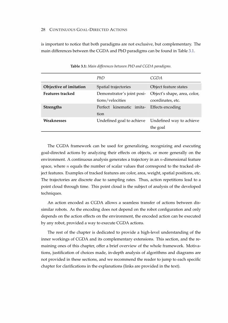
is important to notice that both paradigms are not exclusive, but complementary. The
main differences between the CGDA and PbD paradigms can be found in Table 3.1.
Table 3.1: Main differences between PbD and CGDA paradigms.
PbD CGDA
Objective of imitation Spatial trajectories Object feature states
Features tracked Demonstrator’s joint posi-
tions/velocities
Object’s shape, area, color,
coordinates, etc.
Strengths Perfect kinematic imita-
tion
Effects encoding
Weaknesses Undefined goal to achieve Undefined way to achieve
the goal
The CGDA framework can be used for generalizing, recognizing and executing
goal-directed actions by analyzing their effects on objects, or more generally on the
environment. A continuous analysis generates a trajectory in an n-dimensional feature
space, where n equals the number of scalar values that correspond to the tracked ob-
ject features. Examples of tracked features are color, area, weight, spatial positions, etc.
The trajectories are discrete due to sampling rates. Thus, action repetitions lead to a
point cloud through time. This point cloud is the subject of analysis of the developed
techniques.
An action encoded as CGDA allows a seamless transfer of actions between dis-
similar robots. As the encoding does not depend on the robot configuration and only
depends on the action effects on the environment, the encoded action can be executed
by any robot, provided a way to execute CGDA actions.
The rest of the chapter is dedicated to provide a high-level understanding of the
inner workings of CGDA and its complementary extensions. This section, and the re-
maining ones of this chapter, offer a brief overview of the whole framework. Motiva-
tions, justification of choices made, in-depth analysis of algorithms and diagrams are
not provided in these sections, and we recommend the reader to jump to each specific
chapter for clarifications in the explanations (links are provided in the text).
3.2 SELECTING RELEVANT DEMONSTRATIONS AND FEATURES 29
3.2 Selecting Relevant Demonstrations and Features
As stated previously, the set of demonstrations provided by the user, may include
inadequate demonstrations and unnecessary features. A logical step is to include a
block previous to the generalization block to filter them.
From the raw data, the logical temporal order of screening is to first discard un-
wanted demonstrations, and then select the relevant features. Let us explain why. If
the feature selection were performed in the first place, features from erroneous demon-
strations would influence the results, potentially discarding relevant features and con-
serving irrelevant ones. See 4.2 and 4.3.
One may argue that by first screening the demonstrations, the opposite argument
could be presented. It is undeniable that irrelevant features influence the demonstra-
tion selection. However, from our experience, if a demonstration is performed incor-
rectly, it influences many features in a noticeable way. This empirical fact facilitates the
detection of the most different demonstrations of the set.
3.3 Basic CGDA Framework
Any complete goal-directed framework has to include, at least:
• A generalization module, to create a representative model of the task.
• A recognition module, to be able to measure the similarity of two tasks.
• An execution module, to reproduce an action.
The basic framework flows as follows: Human demonstrations are represented by
a sequence of discrete points in the feature space. The set of demonstrated action rep-
etitions leads to a point cloud in the feature space. A representative feature trajectory is
extracted from the cloud. This feature trajectory represents changes produced in the
object features when an action is performed on it. Generalization is composed by the
following three steps.
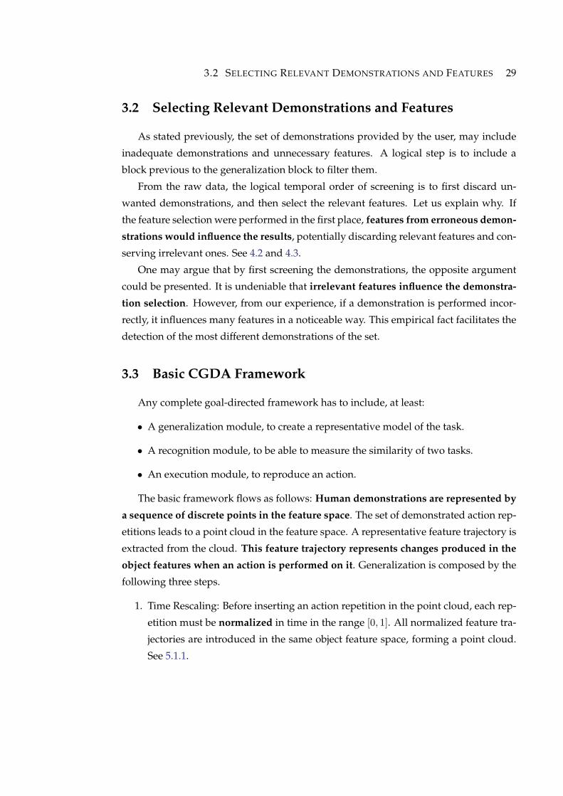
1. Time Rescaling: Before inserting an action repetition in the point cloud, each rep-
etition must be normalized in time in the range [0, 1]. All normalized feature tra-
jectories are introduced in the same object feature space, forming a point cloud.
See 5.1.1.
30 CONTINUOUS GOAL-DIRECTED ACTIONS
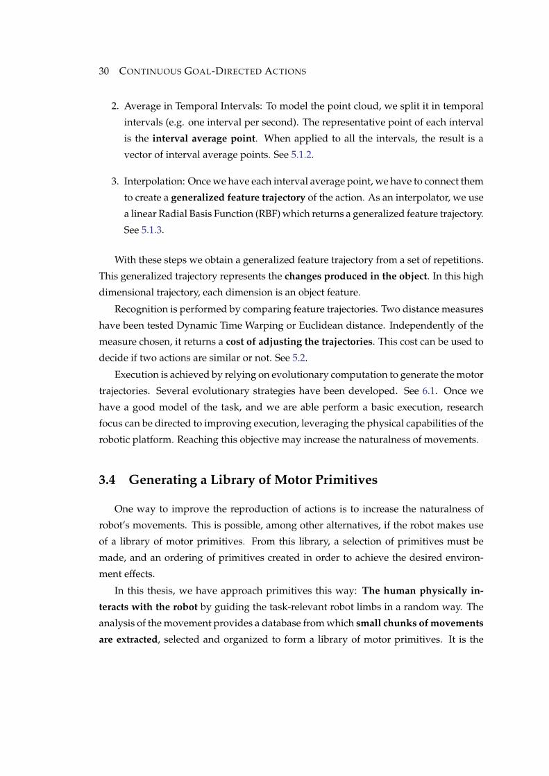
2. Average in Temporal Intervals: To model the point cloud, we split it in temporal
intervals (e.g. one interval per second). The representative point of each interval
is the interval average point. When applied to all the intervals, the result is a
vector of interval average points. See 5.1.2.
3. Interpolation: Once we have each interval average point, we have to connect them
to create a generalized feature trajectory of the action. As an interpolator, we use
a linear Radial Basis Function (RBF) which returns a generalized feature trajectory.
See 5.1.3.
With these steps we obtain a generalized feature trajectory from a set of repetitions.
This generalized trajectory represents the changes produced in the object. In this high
dimensional trajectory, each dimension is an object feature.
Recognition is performed by comparing feature trajectories. Two distance measures
have been tested Dynamic Time Warping or Euclidean distance. Independently of the
measure chosen, it returns a cost of adjusting the trajectories. This cost can be used to
decide if two actions are similar or not. See 5.2.
Execution is achieved by relying on evolutionary computation to generate the motor
trajectories. Several evolutionary strategies have been developed. See 6.1. Once we
have a good model of the task, and we are able perform a basic execution, research
focus can be directed to improving execution, leveraging the physical capabilities of the
robotic platform. Reaching this objective may increase the naturalness of movements.
3.4 Generating a Library of Motor Primitives
One way to improve the reproduction of actions is to increase the naturalness of
robot’s movements. This is possible, among other alternatives, if the robot makes use
of a library of motor primitives. From this library, a selection of primitives must be
made, and an ordering of primitives created in order to achieve the desired environ-
ment effects.
In this thesis, we have approach primitives this way: The human physically in-
teracts with the robot by guiding the task-relevant robot limbs in a random way. The
analysis of the movement provides a database from which small chunks of movements
are extracted, selected and organized to form a library of motor primitives. It is the
3.5 COMPENSATING FRICTION AND GRAVITY 31
combination of these primitives that generate the correct movements to complete the
tasks.
To select and order the primitives, an algorithm has been developed. This algorithm
is a custom tree search algorithm. Topologically, each node represents a primitive, and
each edge is the cost of executing the primitives from the initial node to the current
one. This cost is evaluated in a simulator. See 6.2.
To generate the primitives in this way, the human has to physically move the robot.
Unfortunately, most humanoid robots are heavy and present high friction, due to the
reduction gears and the mechanical elements. Additional controllers with friction and
gravity compensation terms are needed to provide a more natural, and more comfort-
able, fashion to generate motor primitives.
3.5 Compensating Friction and Gravity
Controllers have been developed that alleviate the burden of motor primitive cre-
ation. It is important to notice that these controllers are partial compensators that use
simple friction and gravity models. This thesis considers the use-case of Program-
ming by Demonstration and the controllers are adapted to this scenario. They are
adequate controllers for low joints velocities.
Two controllers have been designed. The Low-Friction Zero-Gravity controller al-
lows a guidance of the robot without effort, allowing small friction forces to reduce
the free robot motion. It can serve to aid users providing kinesthetic demonstrations
while programming by demonstration. In the present, kinesthetic demonstrations are
usually aided by pure gravity compensators, and users must deal with friction.
A Zero-Friction Zero-Gravity controller results in pseudo-free movements, as if the
robot were moving without friction or gravity influence. Ideally, only inertia drives the
movements when zeroing the forces of friction and gravity. In reality, this controller is
able to maintain this behavior up to the joint limit. It is probably not modeling the
friction well enough to maintain the movement indefinitely. Coriolis and centrifugal
forces are depreciated.
The review presented in this chapter can help the reader in understanding the
framework from a high-level perspective. It may also serve as a summary to be con-
sulted if the explanations saturate the reader comprehension in the following chapters.

32 CONTINUOUS GOAL-DIRECTED ACTIONS
34 DEMONSTRATION AND FEATURE SELECTION
• Continuous Goal-Directed Actions (Morante, Victores, Jardon, & Balaguer, 2014)
encodes a generalized action as a feature trajectory preserving all the scalars that
can be extracted from the sensor data at each instant.
Proposition 2 Attending to the space where the generalized model is stored, a handcrafted
feature selection process is implicitly performed when defining the structure of the generalized
model of the task.
While reducing an action to the joint or operational space is a clear over simplifica-
tion for many use cases (e.g. filling a glass depends on the layout of the environment),
preserving all the scalar features that can be extracted from the sensor data can lead
to not knowing which feature is relevant for the task. For instance, a person fills a
glass with water by pouring it from a bottle. Which are the features that are relevant
for the task? The area of the glass that is perceived with a slightly different color due
to the new refraction index? The absolute or relative position and orientation of the
bottle? Reproducing the sound of a motorcycle that was passing by during one of the
demonstrations?
For this problem, this thesis presents a solution: choose as relevant signals (fea-
tures or demonstrations) those consistent among task repetitions. This dilemma, de-
ciding if a consistent signal is relevant or not, dates back to Newton’s Philosophiae
Naturalis Principia Mathematica (Newton, Bernoulli, MacLaurin, & Euler, 1833). In his
book, in addition to introducing the law of universal gravitation, Newton stated four
rules of reasoning in philosophy, which can be called rules of induction because of their
content. Newton offered a methodology for dealing with unknown phenomena and
building explanations for them:
1. We are to admit no more causes of natural things than such as are both
true and sufficient to explain their appearances.
2. Therefore to the same natural effects we must, as far as possible, assign
the same causes.
3. The qualities of bodies, which admit neither intensification nor re-
mission of degrees, and which are found to belong to all bodies
within the reach of our experiments, are to be esteemed the universal
qualities of all bodies whatsoever.
4.1 DISSIMILARITY MAPPING FILTERING 35
4. In experimental philosophy we are to look upon propositions inferred
by general induction from phenomena as accurately or very nearly
true, not withstanding any contrary hypothesis that may be imagined,
till such time as other phenomena occur, by which they may either be
made more accurate, or liable to exceptions.
Specially interesting for our problem is the rule number three. Rephrasing it in
modern language, it says:
Whatever holds true for every case we have seen, holds true for all the other
cases.
This rule is at the heart of many (if not all) machine learning algorithms, and it is
also of our selection process. In this thesis, a machine learning process for variable
selection is presented. The process is called Dissimilarity Mapping Filtering (DMF).
DMF is flexible in its design, allowing different algorithms in each of its blocks. DMF
is applied for demonstration selection and for feature selection.
4.1 Dissimilarity Mapping Filtering
The Dissimilarity Mapping Filtering process (DMF), applied as a demonstration se-
lector and as a feature selector (Morante, Victores, & Balaguer, 2015a), is introduced in
this section. An additional preprocessing step is incorporated in the descriptions prior
to the dissimilarity, mapping, and filtering steps. A visual example of a generic DMF
use is shown in Figure 4.2. In this picture, the term signal represents either demonstra-
tions or features.
Despite the DMF process is generic, non-specific for robot learning, and can be ap-
plied to other problems, we aim at solving a problem in a target scenario. We work in
a robotics learning scenario, using a humanoid robot equipped with simple 3D vision,
learning a block-moving task (see Figure 4.3).
4.2 Demonstration Selector
Using DMF as a demonstration selector, the goal of the process is to automati-
cally discard incorrectly sensed or performed demonstrations. Assuming each fea-
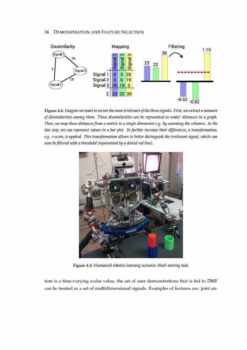
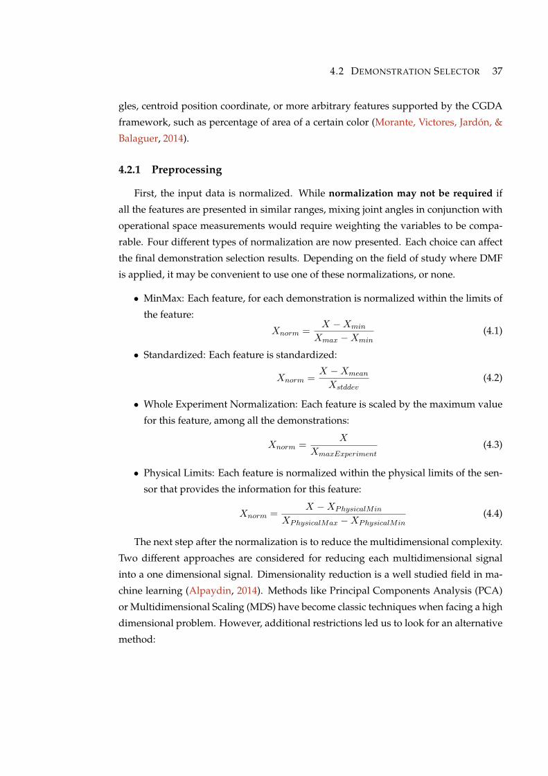
4.2 DEMONSTRATION SELECTOR 37
gles, centroid position coordinate, or more arbitrary features supported by the CGDA
framework, such as percentage of area of a certain color (Morante, Victores, Jardon, &
Balaguer, 2014).
4.2.1 Preprocessing
First, the input data is normalized. While normalization may not be required if
all the features are presented in similar ranges, mixing joint angles in conjunction with
operational space measurements would require weighting the variables to be compa-
rable. Four different types of normalization are now presented. Each choice can affect
the final demonstration selection results. Depending on the field of study where DMF
is applied, it may be convenient to use one of these normalizations, or none.
• MinMax: Each feature, for each demonstration is normalized within the limits of
the feature:
Xnorm =X −Xmin
Xmax −Xmin(4.1)
• Standardized: Each feature is standardized:
Xnorm =X −Xmean
Xstddev(4.2)
• Whole Experiment Normalization: Each feature is scaled by the maximum value
for this feature, among all the demonstrations:
Xnorm =X
XmaxExperiment(4.3)
• Physical Limits: Each feature is normalized within the physical limits of the sen-
sor that provides the information for this feature:
Xnorm =X −XPhysicalMin
XPhysicalMax −XPhysicalMin(4.4)
The next step after the normalization is to reduce the multidimensional complexity.
Two different approaches are considered for reducing each multidimensional signal
into a one dimensional signal. Dimensionality reduction is a well studied field in ma-
chine learning (Alpaydin, 2014). Methods like Principal Components Analysis (PCA)
or Multidimensional Scaling (MDS) have become classic techniques when facing a high
dimensional problem. However, additional restrictions led us to look for an alternative
method:
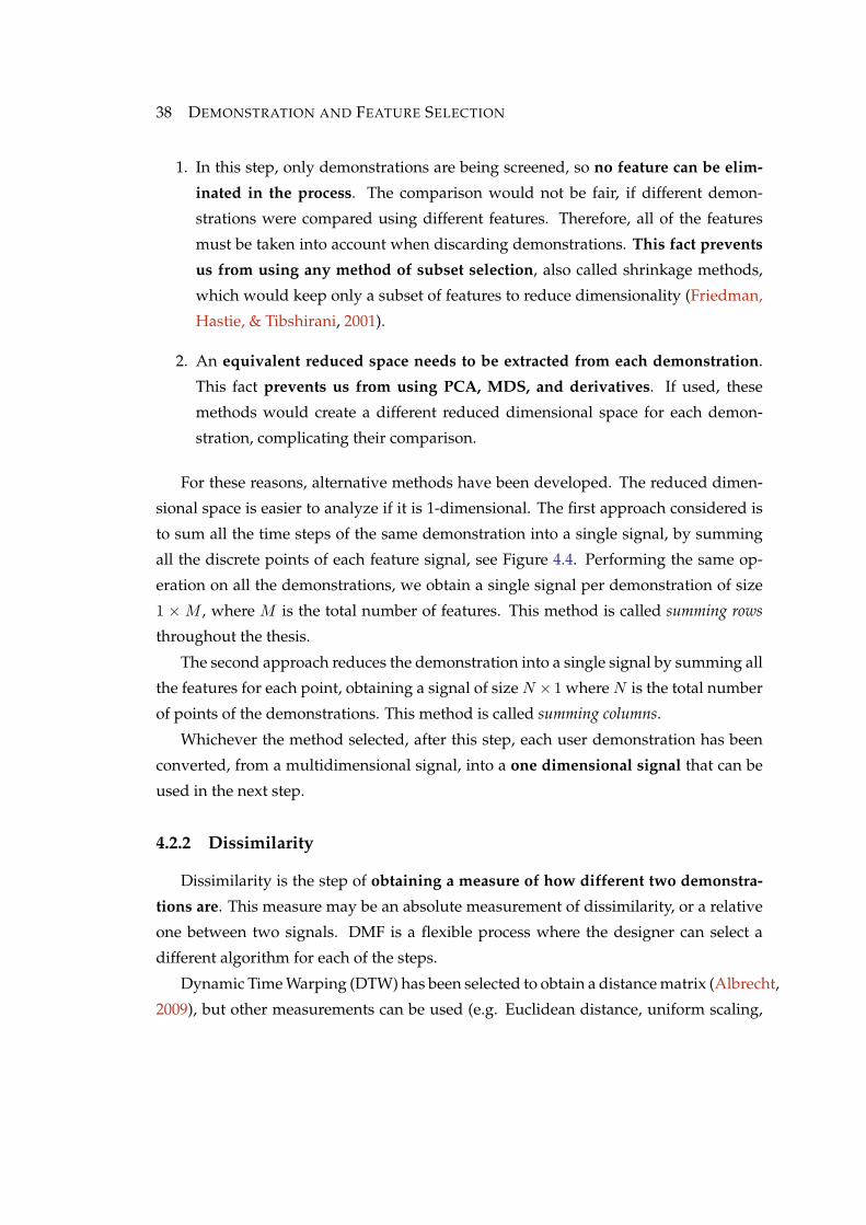
38 DEMONSTRATION AND FEATURE SELECTION
1. In this step, only demonstrations are being screened, so no feature can be elim-
inated in the process. The comparison would not be fair, if different demon-
strations were compared using different features. Therefore, all of the features
must be taken into account when discarding demonstrations. This fact prevents
us from using any method of subset selection, also called shrinkage methods,
which would keep only a subset of features to reduce dimensionality (Friedman,
Hastie, & Tibshirani, 2001).
2. An equivalent reduced space needs to be extracted from each demonstration.
This fact prevents us from using PCA, MDS, and derivatives. If used, these
methods would create a different reduced dimensional space for each demon-
stration, complicating their comparison.
For these reasons, alternative methods have been developed. The reduced dimen-
sional space is easier to analyze if it is 1-dimensional. The first approach considered is
to sum all the time steps of the same demonstration into a single signal, by summing
all the discrete points of each feature signal, see Figure 4.4. Performing the same op-
eration on all the demonstrations, we obtain a single signal per demonstration of size
1 ×M , where M is the total number of features. This method is called summing rows
throughout the thesis.
The second approach reduces the demonstration into a single signal by summing all
the features for each point, obtaining a signal of size N × 1 where N is the total number
of points of the demonstrations. This method is called summing columns.
Whichever the method selected, after this step, each user demonstration has been
converted, from a multidimensional signal, into a one dimensional signal that can be
used in the next step.
4.2.2 Dissimilarity
Dissimilarity is the step of obtaining a measure of how different two demonstra-
tions are. This measure may be an absolute measurement of dissimilarity, or a relative
one between two signals. DMF is a flexible process where the designer can select a
different algorithm for each of the steps.
Dynamic Time Warping (DTW) has been selected to obtain a distance matrix (Albrecht,
2009), but other measurements can be used (e.g. Euclidean distance, uniform scaling,
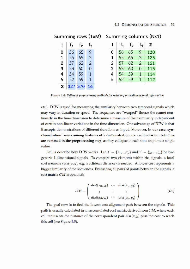
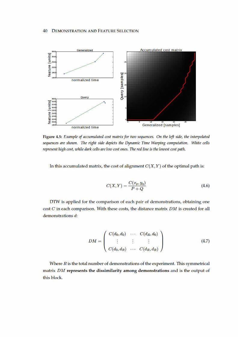

4.2 DEMONSTRATION SELECTOR 41
4.2.3 Mapping
The main idea in this step is to reduce the information provided by the previous
step, which is a matrix, into a single scalar value per demonstration. This reduction
can be considered a mapping into a lower dimensional space.
Let us remind what this matrix is. Each cell i, j in the matrix represents the dis-
similarity between the demonstration i and the demonstration j. When i = j, this
dissimilarity will be, obviously, zero.
The aim is to compress into a single value, how dissimilar a demonstration is with
respect to the rest of the demonstrations of the set. The matrix DM provides this in-
formation by collapsing (summing) its rows or columns (being both results equal as the
matrix is symmetrical). In an alternative interpretation, if the signals are imagined as
nodes in a graph, the dissimilarity between two signals is the “distance” that separates
them, as shown in Fig. 4.2. By summing all the distances from a single node, to all the
other nodes, we are capturing how far this signal is from the rest of signals.
We have chosen to map the distance matrix DM into a single dimension by sum-
ming the values in the columns, but other algorithms can be used, e.g. multidimen-
sional scaling, ISOMAP, etc. With our method, a value V is obtained for each demon-
stration i:
Vi =R∑
j=0
C(di, dj) (4.8)
Each value V represents a measurement of the dissimilarity of a demonstration
with respect to all the others, and R is the total number of demonstrations. The set of
measurements of dissimilarity is the returned data of this block.
4.2.4 Filtering
In this last step, the aim is to screen the demonstrations, to discard the outlying
ones. If previous algorithms have been correctly designed and selected, and have not
distorted the information contained in the demonstrations, there should be possible to
isolate the most different ones of the set.
We have chosen to filter them by using the z-score (called standard score) because
it standardizes the results, but other algorithms can be used: DBSCAN, t-test, etc. In
42 DEMONSTRATION AND FEATURE SELECTION
fact, any algorithms able to isolate outliers in one dimension can be applied. In case the
standard score is selected, each value V is converted into a z-score Z:
Z =V − Vmean
Vstddev(4.9)
Finally, the demonstrations with a z-scoreZ higher than a threshold α are discarded.
In common statistical outliers detection, the positive threshold has a symmetrical equiv-
alent on the negative side, to discard the values lower than the negative threshold. In
the filter presented in this section, there is no need of a symmetrical threshold. The rea-
son is that values to be standardized represent dissimilarities, and we are only looking
for the biggest dissimilarities of the set. This threshold α is the only tunable parameter
of the whole DMF process, if the designer chooses the same algorithms as in this thesis.
The use of z-score as filtering method implies accepting an assumption in the data:
there are enough relevant signals (in this case, demonstrations) in the set to compensate
the effect of irrelevant ones. The reason behind this assumption is that in the process
of subtracting the mean to all the values, it may occur that an abundance of irrelevant
demonstrations rises up the mean value, mitigating the effect of the transformation,
and allowing irrelevant signals to be considered as relevant.
This assumption should not be a problem for demonstration selection, because if a
user is demonstrating a task to a robot, and most of the demonstrations are incorrect,
maybe this user is not the best teacher for the robot. A possible approach for solving
this problem would be to apply iteratively the filtering algorithm several times (two
times should be enough for most cases). It will reduce the number of irrelevant signals,
but may potentially discard relevant ones if it is applied many times.
This preprocessing, dissimilarity, mapping and filtering process, discards the incor-
rect demonstrations. Once the set of demonstration is curated, it is possible to filter
irrelevant features. In the next section, how to discard irrelevant features using DMF is
explained.
4.3 Feature Selector
The goal of this section is to discard those features not relevant for a specific task.
We start again from the raw data, but using only the correct demonstrations selected in
the previous step. This machine learning pipeline is automatic, as each step can feed the
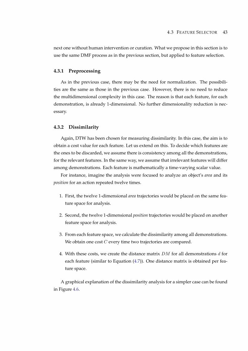
4.3 FEATURE SELECTOR 43
next one without human intervention or curation. What we propose in this section is to
use the same DMF process as in the previous section, but applied to feature selection.
4.3.1 Preprocessing
As in the previous case, there may be the need for normalization. The possibili-
ties are the same as those in the previous case. However, there is no need to reduce
the multidimensional complexity in this case. The reason is that each feature, for each
demonstration, is already 1-dimensional. No further dimensionality reduction is nec-
essary.
4.3.2 Dissimilarity
Again, DTW has been chosen for measuring dissimilarity. In this case, the aim is to
obtain a cost value for each feature. Let us extend on this. To decide which features are
the ones to be discarded, we assume there is consistency among all the demonstrations,
for the relevant features. In the same way, we assume that irrelevant features will differ
among demonstrations. Each feature is mathematically a time-varying scalar value.
For instance, imagine the analysis were focused to analyze an object’s area and its
position for an action repeated twelve times.
1. First, the twelve 1-dimensional area trajectories would be placed on the same fea-
ture space for analysis.
2. Second, the twelve 1-dimensional position trajectories would be placed on another
feature space for analysis.
3. From each feature space, we calculate the dissimilarity among all demonstrations.
We obtain one cost C every time two trajectories are compared.
4. With these costs, we create the distance matrix DM for all demonstrations d for
each feature (similar to Equation (4.7)). One distance matrix is obtained per fea-
ture space.
A graphical explanation of the dissimilarity analysis for a simpler case can be found
in Figure 4.6.

4.3 FEATURE SELECTOR 45
4.3.4 Filtering
The filtering process is again performed using z-scores. Each value Vtotal is con-
verted to a z-score Z, and the algorithm discards the features with a z-score Z higher
than an α threshold.
As in the previous case, the use of z-score as filtering method implies there are
enough relevant signals (in this case, features) to compensate the effect of irrelevant
ones. This assumption may potentially be a problem for feature selection. If a system
is endowed with very general task-independent features, it is reasonable to think that
most of them will not be relevant for a specific task. The solution offered in this case
is again, to apply iteratively the filtering algorithm several times. Another obvious
solution for these cases is to use another algorithm in the filtering block.
After this whole process of demonstration and feature selection, a clean and curated
dataset has been obtained, and the CGDA analysis can be carried out.

46 DEMONSTRATION AND FEATURE SELECTION
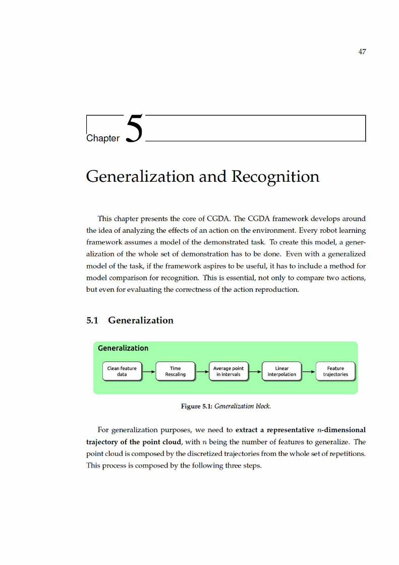

48 GENERALIZATION AND RECOGNITION
5.1.1 Time Rescaling
Before inserting a single action repetition in the point cloud, it is normalized in time
(range [0, 1]). With this time rescaling, every action demonstration gets bounded by
the same temporal limits, making the algorithm independent of the repetitions’ speed.
While this decision simplifies the posterior analysis, it makes a potential execution un-
aware of the task’s speed. A preprogrammed execution speed should be provided, or
speed itself should be considered as an input feature to the system. All normalized
trajectories are introduced in a feature space, forming a point cloud.
5.1.2 Average in Temporal Intervals
To model the point cloud, we split it in temporal intervals, fixing one interval per
second. The number of seconds is computed from the average duration of the original
repetitions. Each interval contains points of all repetitions, in the same percentage of
execution. As the repetitions are normalized in time, each interval represents a percent-
age of action execution, and the number of intervals allows preserving a notion of the
action duration. The representative point p of each interval is extracted as:
p =1
pint
pint∑i=0
Xi (5.1)
Where pint is the number of points in the interval and Xi represent the vector of fea-
tures for a point. In other words, this representative point of each interval is extracted
as the average for each dimension of all points of the interval, as seen in Figure 5.2.
The result is a vector of average features. These temporal averaged points are the ones
used in the posterior interpolation.
5.1.3 Radial Basis Function Interpolation
Once the representative points of the point cloud are obtained, they have to be
joined to create a generalized action model, i.e. an object feature trajectory we can
consider as a generalization. In a robot joint space, an interpolation could create a jerky
joint trajectory, so literature, e.g. (Calinon et al., 2010), commonly uses regressors such
as Gaussian Mixture Regression. However, working in the object feature space, we use
an interpolator to assure the trajectories pass through the target points (which are the
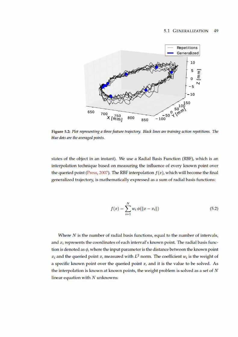
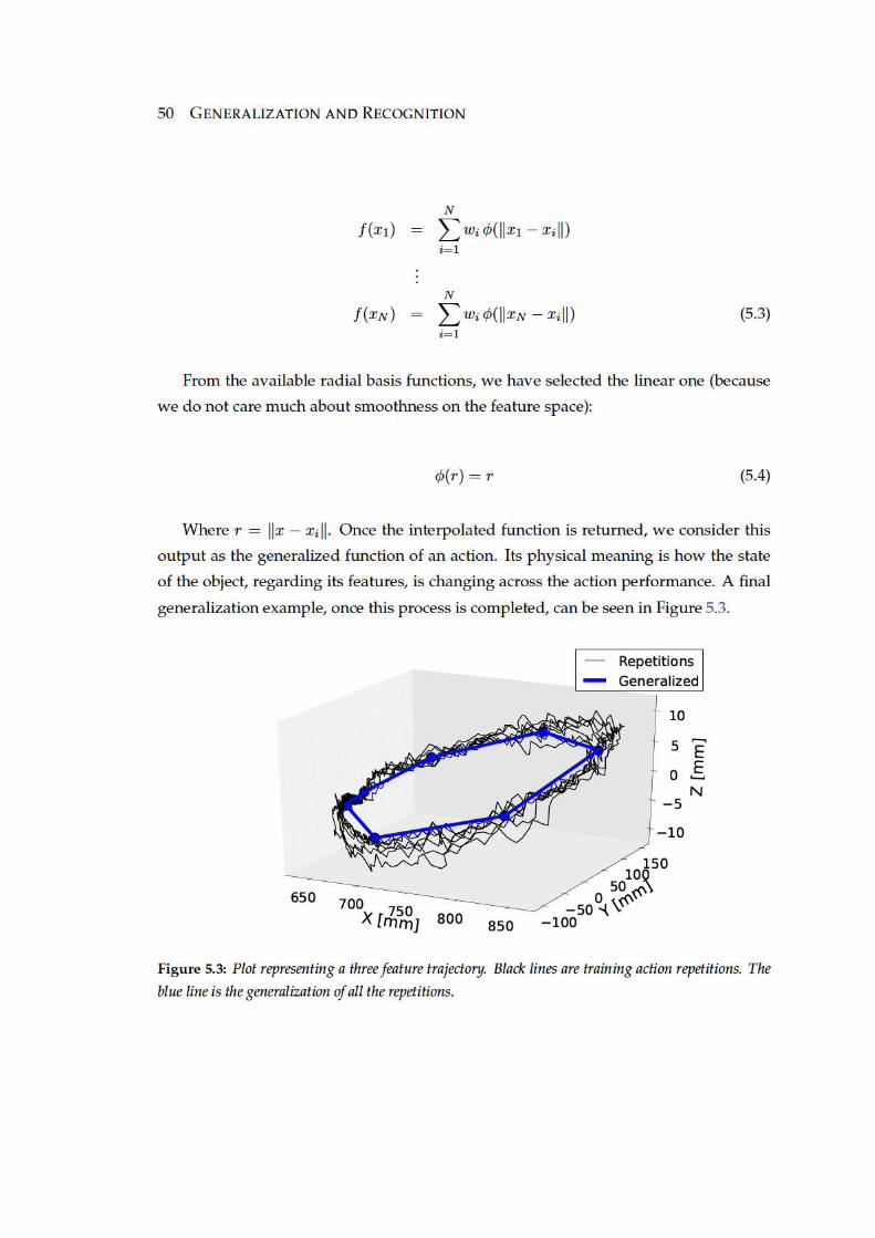
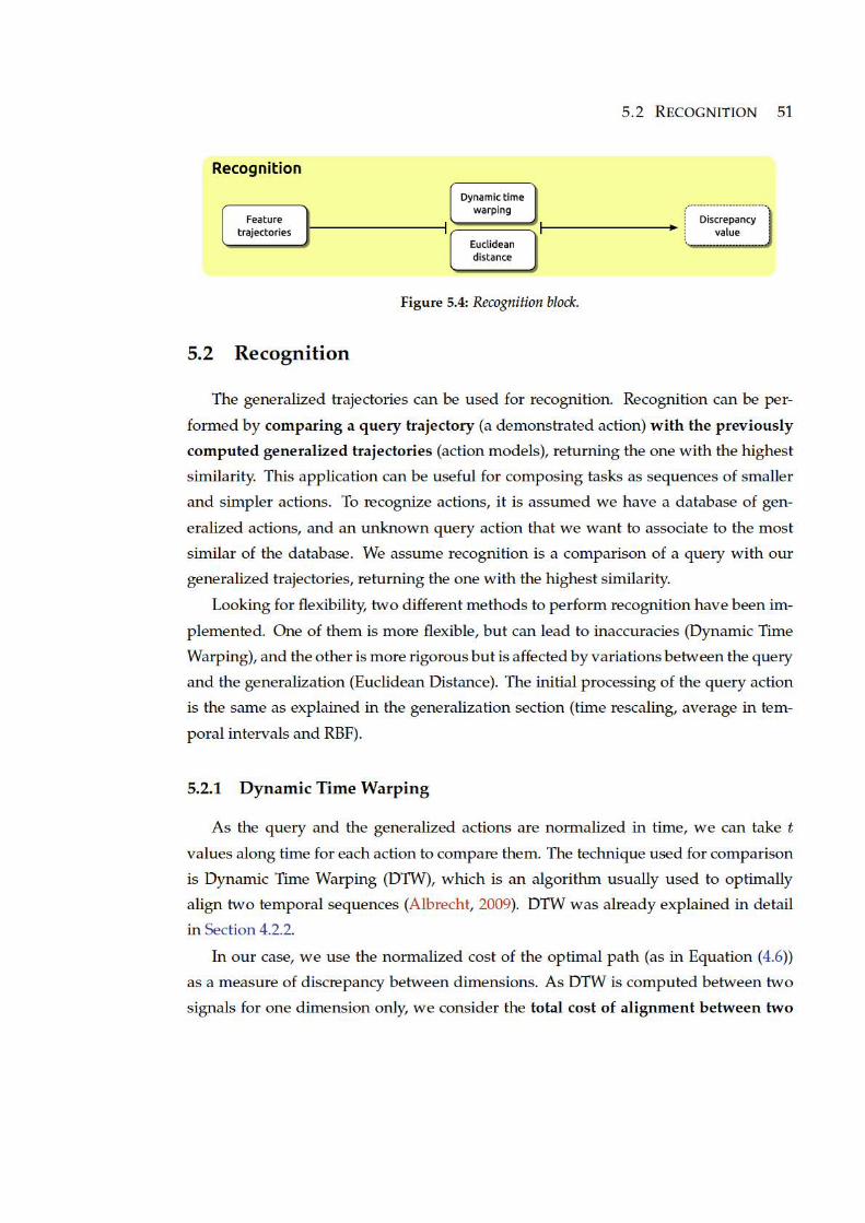
52 GENERALIZATION AND RECOGNITION
n-dimensional trajectories as the sum of the costs of the optimal paths of each di-
mension, obtaining a single score D:
D =n∑
i=1
CPnorm(Xi, Yi) (5.5)
This score is used as the measure of discrepancy between two trajectories in the
n-dimensional space. In recognition, the trajectory with the smallest score is the one we
consider the match.
5.2.2 Euclidean Distance
Another option to perform recognition, or in general, to measure the error between
two trajectories, is to use the Euclidean distance. The query trajectory is normalized in
time, in the same way it was for the generalized ones. This step allows us to take t val-
ues along time for each action (the query and the generalized) to compare them. The use
of DTW is motivated to allow a non-rigid measure of similarity between trajectories, as
DTW is able to ‘tighten’ and ‘widen’ until both are best aligned. Unfortunately, DTW
allows time displacements that can affect the order of execution of actions, resulting in
task failure or performance decay. Therefore, Euclidean distance can be considered an
improvement with respect to DTW as metric.
Our aim when using Euclidean distance is to obtain a metric of discrepancy be-
tween two time-dependent sequences of points, namely X = {x1, .., xN} and Y =
{y1, .., yN}. We compute the total discrepancy J(X,Y ) between two n-dimensional tra-
jectories as:
J(X,Y ) = ‖X − Y ‖ (5.6)
The generalized trajectory with the smallest J(X,Y ) is the one we consider as the
most similar. Let us recall that all the trajectories involved in this process of recognition
are feature trajectories and not joint space trajectories. This implies that we are recog-
nizing actions by what is happening to the object, and not comparing human move-
ments.
The differences in comparison of signals between Dynamic Time Warping and Eu-
clidean distance can be seen in Figure 5.5.
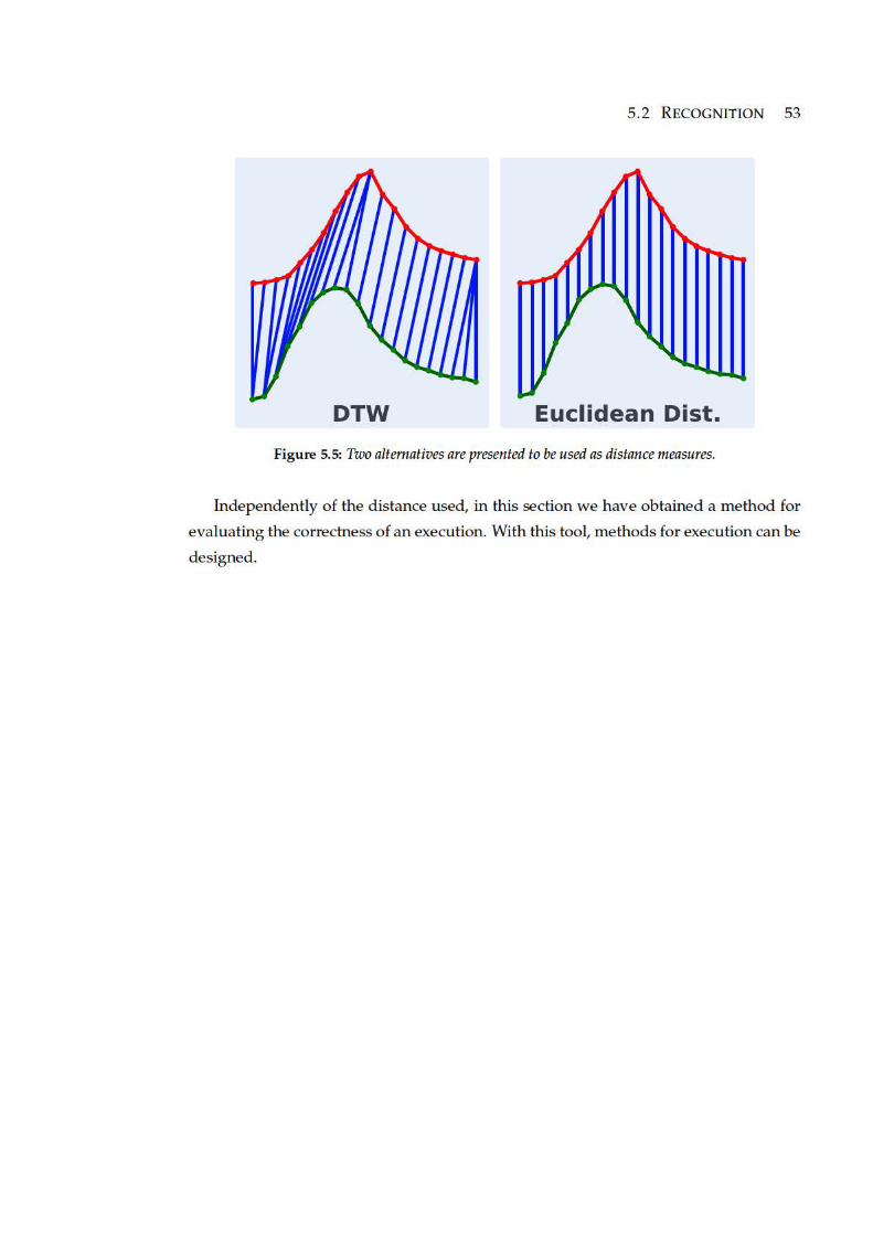

54 GENERALIZATION AND RECOGNITION
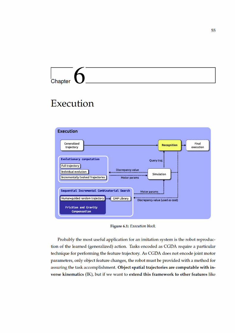
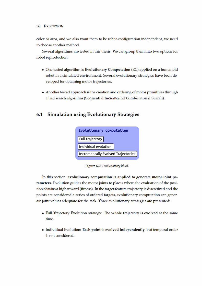
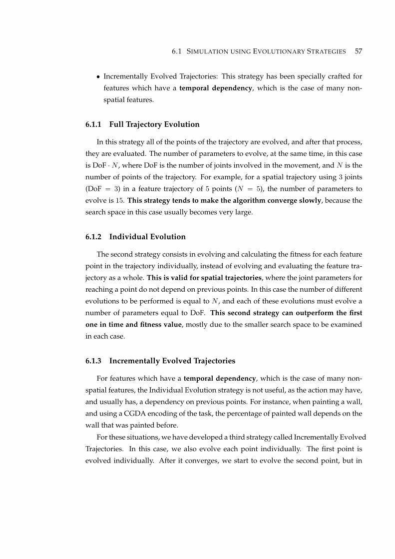
6.1 SIMULATION USING EVOLUTIONARY STRATEGIES 57
• Incrementally Evolved Trajectories: This strategy has been specially crafted for
features which have a temporal dependency, which is the case of many non-
spatial features.
6.1.1 Full Trajectory Evolution
In this strategy all of the points of the trajectory are evolved, and after that process,
they are evaluated. The number of parameters to evolve, at the same time, in this case
is DoF ·N , where DoF is the number of joints involved in the movement, and N is the
number of points of the trajectory. For example, for a spatial trajectory using 3 joints
(DoF = 3) in a feature trajectory of 5 points (N = 5), the number of parameters to
evolve is 15. This strategy tends to make the algorithm converge slowly, because the
search space in this case usually becomes very large.
6.1.2 Individual Evolution
The second strategy consists in evolving and calculating the fitness for each feature
point in the trajectory individually, instead of evolving and evaluating the feature tra-
jectory as a whole. This is valid for spatial trajectories, where the joint parameters for
reaching a point do not depend on previous points. In this case the number of different
evolutions to be performed is equal to N , and each of these evolutions must evolve a
number of parameters equal to DoF. This second strategy can outperform the first
one in time and fitness value, mostly due to the smaller search space to be examined
in each case.
6.1.3 Incrementally Evolved Trajectories
For features which have a temporal dependency, which is the case of many non-
spatial features, the Individual Evolution strategy is not useful, as the action may have,
and usually has, a dependency on previous points. For instance, when painting a wall,
and using a CGDA encoding of the task, the percentage of painted wall depends on the
wall that was painted before.
For these situations, we have developed a third strategy called Incrementally Evolved
Trajectories. In this case, we also evolve each point individually. The first point is
evolved individually. After it converges, we start to evolve the second point, but in
58 EXECUTION
this case, the fitness evaluation is performed by sequentially executing both points (the
previous first point and the current point). Once the second point converges, we start
evolving the third point and for the evaluation we execute the three point trajectory.
The same process is repeated for the remaining points. The pseudocode of this strategy
is shown in Algorithm 1.
Algorithm 1 Incrementally Evolved Trajectories (IET)
1: procedure IET(X, ε) . X is the feature trajectory. ε is an error parameter.
2: for i < numberOfPoints(X) do
3: while fitness > ε do
4: Mi ←evolve()
5: f ←execute(M[0:i])
6: fitness←compare(f,Xi)
7: end while
8: end for
9: return M
10: end procedure
This technique offers some advantages with respect to the alternative strategies.
First, it reduces the search space for each individual evolution, as it only evolves one
point each time. Second, it also reduces the time necessary to converge, and improves
fitness value of the whole trajectory. In the experimental section, we will show how it
is able to approximate different object feature trajectories.
Moving from evolutionary computation, we realized we can leverage from physical
interaction with the robot. Physical interaction can be translated into motor primitives,
which are then used as pieces of a puzzle. When put in the correct order, primitives
form a joint trajectory. Let us now extend on this idea.
6.2 Guided Motor Primitives
Our work on CGDA execution can be seen as a search of inverse models based on
task goals i.e. compute the action policies that can generate a given effect. We benefit
from human-robot interaction to create a library of Guided Motor Primitives (GMP).
These primitives are created by extracting segments of movements from a random

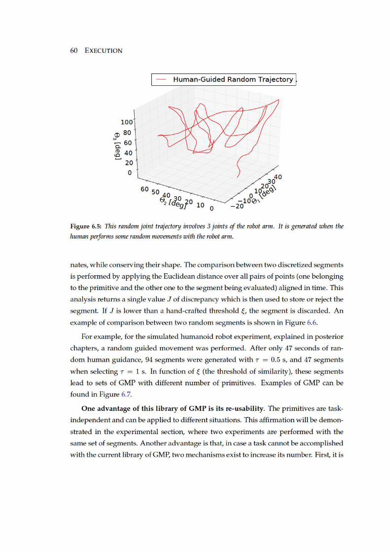
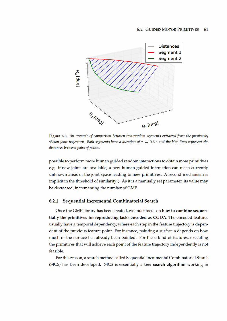
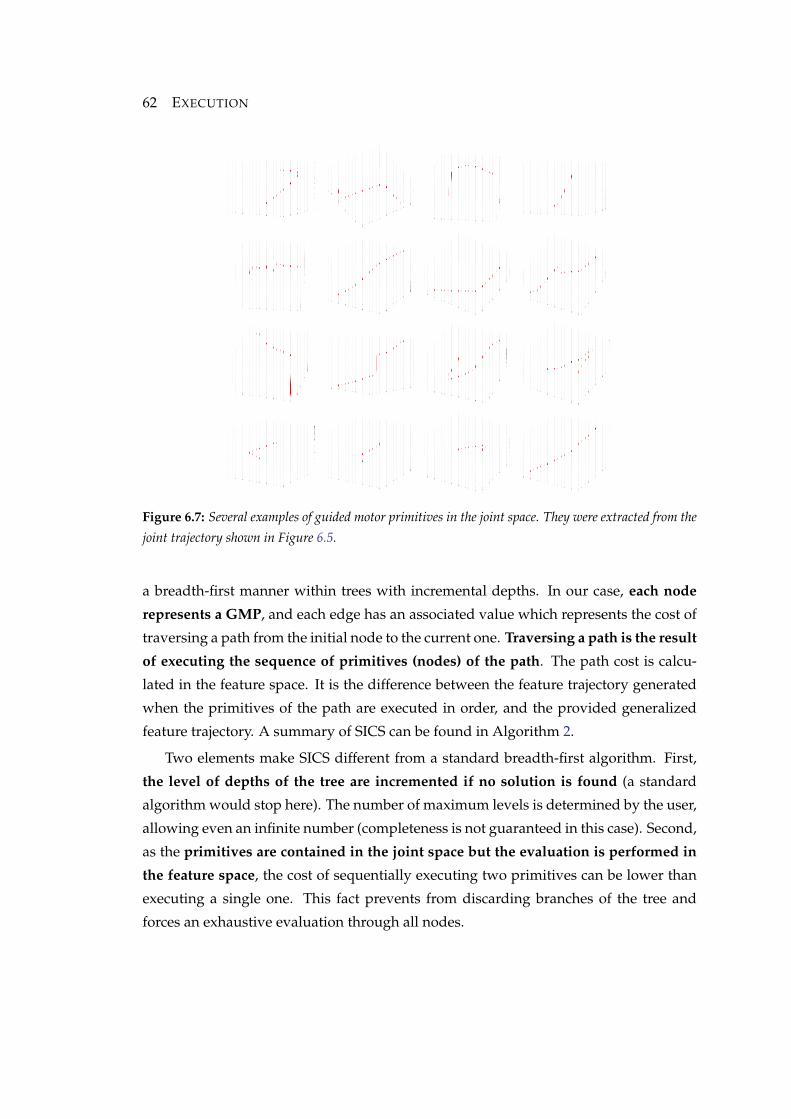
62 EXECUTION
Figure 6.7: Several examples of guided motor primitives in the joint space. They were extracted from the
joint trajectory shown in Figure 6.5.
a breadth-first manner within trees with incremental depths. In our case, each node
represents a GMP, and each edge has an associated value which represents the cost of
traversing a path from the initial node to the current one. Traversing a path is the result
of executing the sequence of primitives (nodes) of the path. The path cost is calcu-
lated in the feature space. It is the difference between the feature trajectory generated
when the primitives of the path are executed in order, and the provided generalized
feature trajectory. A summary of SICS can be found in Algorithm 2.
Two elements make SICS different from a standard breadth-first algorithm. First,
the level of depths of the tree are incremented if no solution is found (a standard
algorithm would stop here). The number of maximum levels is determined by the user,
allowing even an infinite number (completeness is not guaranteed in this case). Second,
as the primitives are contained in the joint space but the evaluation is performed in
the feature space, the cost of sequentially executing two primitives can be lower than
executing a single one. This fact prevents from discarding branches of the tree and
forces an exhaustive evaluation through all nodes.
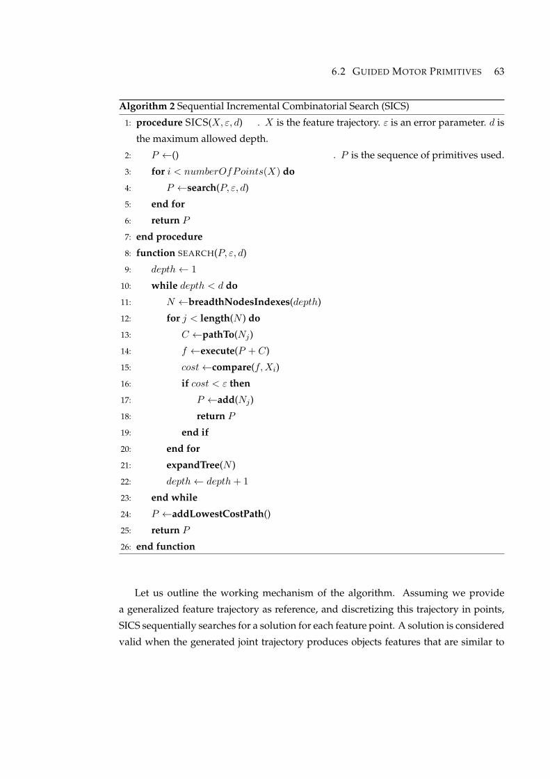
6.2 GUIDED MOTOR PRIMITIVES 63
Algorithm 2 Sequential Incremental Combinatorial Search (SICS)
1: procedure SICS(X, ε, d) . X is the feature trajectory. ε is an error parameter. d is
the maximum allowed depth.
2: P ←() . P is the sequence of primitives used.
3: for i < numberOfPoints(X) do
4: P ←search(P, ε, d)
5: end for
6: return P
7: end procedure
8: function SEARCH(P, ε, d)
9: depth← 1
10: while depth < d do
11: N ←breadthNodesIndexes(depth)
12: for j < length(N ) do
13: C ←pathTo(Nj)
14: f ←execute(P + C)
15: cost←compare(f,Xi)
16: if cost < ε then
17: P ←add(Nj)
18: return P
19: end if
20: end for
21: expandTree(N )
22: depth← depth+ 1
23: end while
24: P ←addLowestCostPath()
25: return P
26: end function
Let us outline the working mechanism of the algorithm. Assuming we provide
a generalized feature trajectory as reference, and discretizing this trajectory in points,
SICS sequentially searches for a solution for each feature point. A solution is considered
valid when the generated joint trajectory produces objects features that are similar to
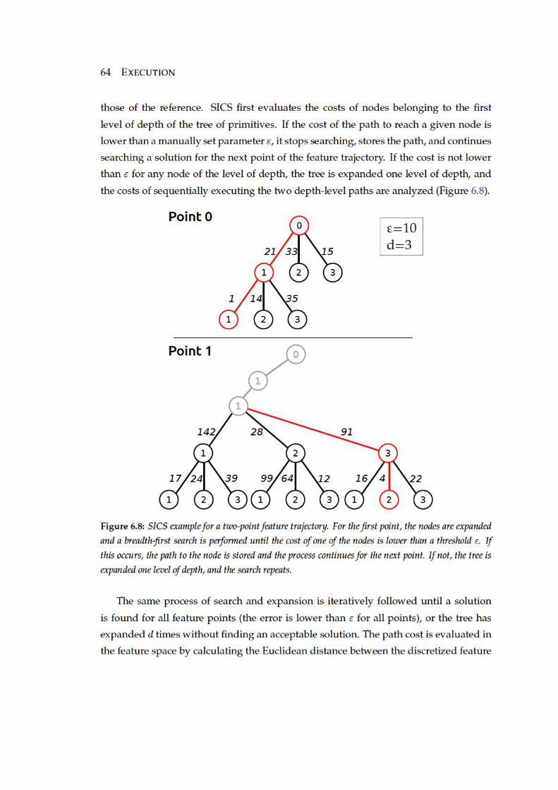
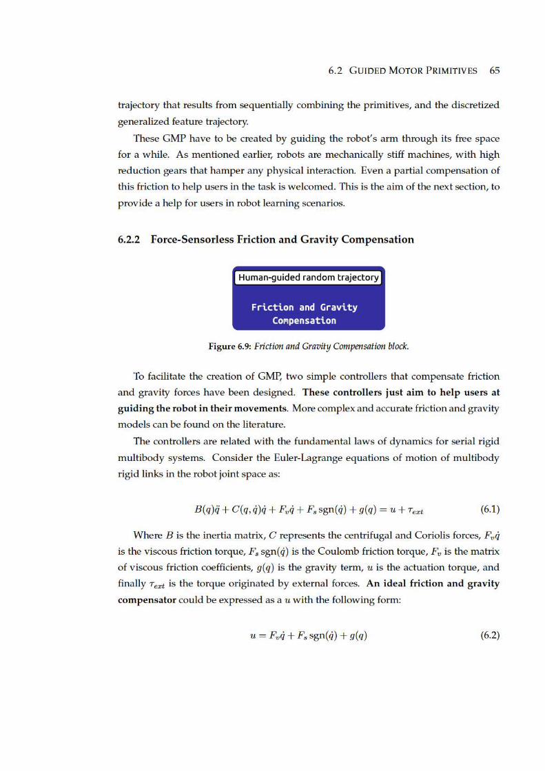
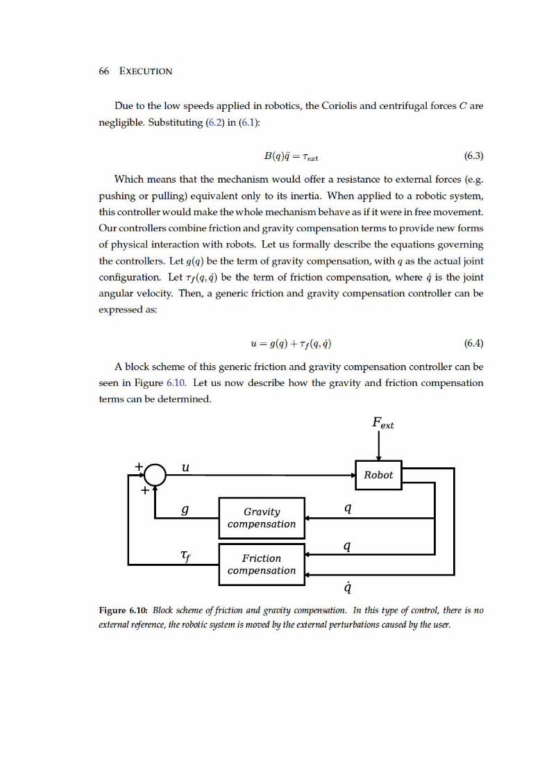
6.2 GUIDED MOTOR PRIMITIVES 67
Gravity Compensation
The potential energy of a robot, assuming rigid links and punctual masses, can be
defined as (Sciavicco & Villani, 2009):
U =n∑
i=1
(Uli + Umi) (6.5)
Where Uli is the sum of potential energy contributions of each link, Umi is the con-
tribution of each motor, and i is an index for each link or motor. The first term Uli is
defined as:
Uli = −mligT0 pli (6.6)
Where mli is the mass of the center of masses of link i, g0 is the gravity vector ex-
pressed in base frame (e.g. g0 = [0 0 − 9.81]T ), and pli is the set of coordinates of the
center of masses of link i expressed in the base frame. Similarly, the motor contributions
Umi are defined as:
Umi = −mmigT0 pmi (6.7)
Substituting (6.6) and (6.7) in (6.5), U becomes:
U = −n∑
i=1
(mligT0 pli +mmig
T0 pmi) (6.8)
Where pli and pmi depend on the joint configuration q. The torque g(q) exerted by
gravity can be computed as (Luca & Panzieri, 1993):
g(q) =∂U
∂q(6.9)
And is thus the torque required for gravity compensation. In the real world, de-
termining the influence of each element in the potential energy equation is a non-trivial
issue. For instance, the distinction between motor and link mass contribution is blurry,
as the mass contribution between motors includes the parts of the motors located be-
tween the axes of rotation. This is the reason why we will use a simplified dynamic
model of U . In this simplified model, the terms of link and motor contributions are
mixed, and their masses are concentrated in the intermediate point between each pair
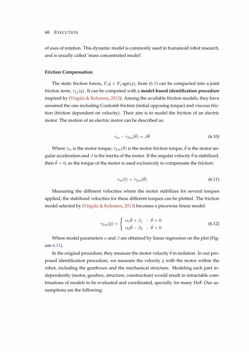
68 EXECUTION
of axes of rotation. This dynamic model is commonly used in humanoid robot research,
and is usually called ‘mass concentrated model’.
Friction Compensation
The static friction forces, Fv q + Fs sgn(q), from (6.1) can be compacted into a joint
friction term, τfj(q). It can be computed with a model-based identification procedure
inspired by (Virgala & Kelemen, 2013). Among the available friction models, they have
assumed the one including Coulomb friction (initial opposing torque) and viscous fric-
tion (friction dependent on velocity). Their aim is to model the friction of an electric
motor. The motion of an electric motor can be described as:
τm − τfm(θ) = Jθ (6.10)
Where τm is the motor torque, τfm(θ) is the motor friction torque, θ is the motor an-
gular acceleration and J is the inertia of the motor. If the angular velocity θ is stabilized,
then θ = 0, so the torque of the motor is used exclusively to compensate the friction:
τm(t) = τfm(θ) (6.11)
Measuring the different velocities where the motor stabilizes for several torques
applied, the stabilized velocities for these different torques can be plotted. The friction
model selected by (Virgala & Kelemen, 2013) becomes a piecewise linear model:
τfm(q) =
{α1θ + β1 : θ > 0
α2θ − β2 : θ < 0(6.12)
Where model parameters α and β are obtained by linear regression on the plot (Fig-
ure 6.11).
In the original procedure, they measure the motor velocity θ in isolation. In our pro-
posed identification procedure, we measure the velocity q with the motor within the
robot, including the gearboxes and the mechanical structure. Modeling each part in-
dependently (motor, gearbox, structure, construction) would result in intractable com-
binations of models to be evaluated and coordinated, specially for many DoF. Our as-
sumptions are the following:
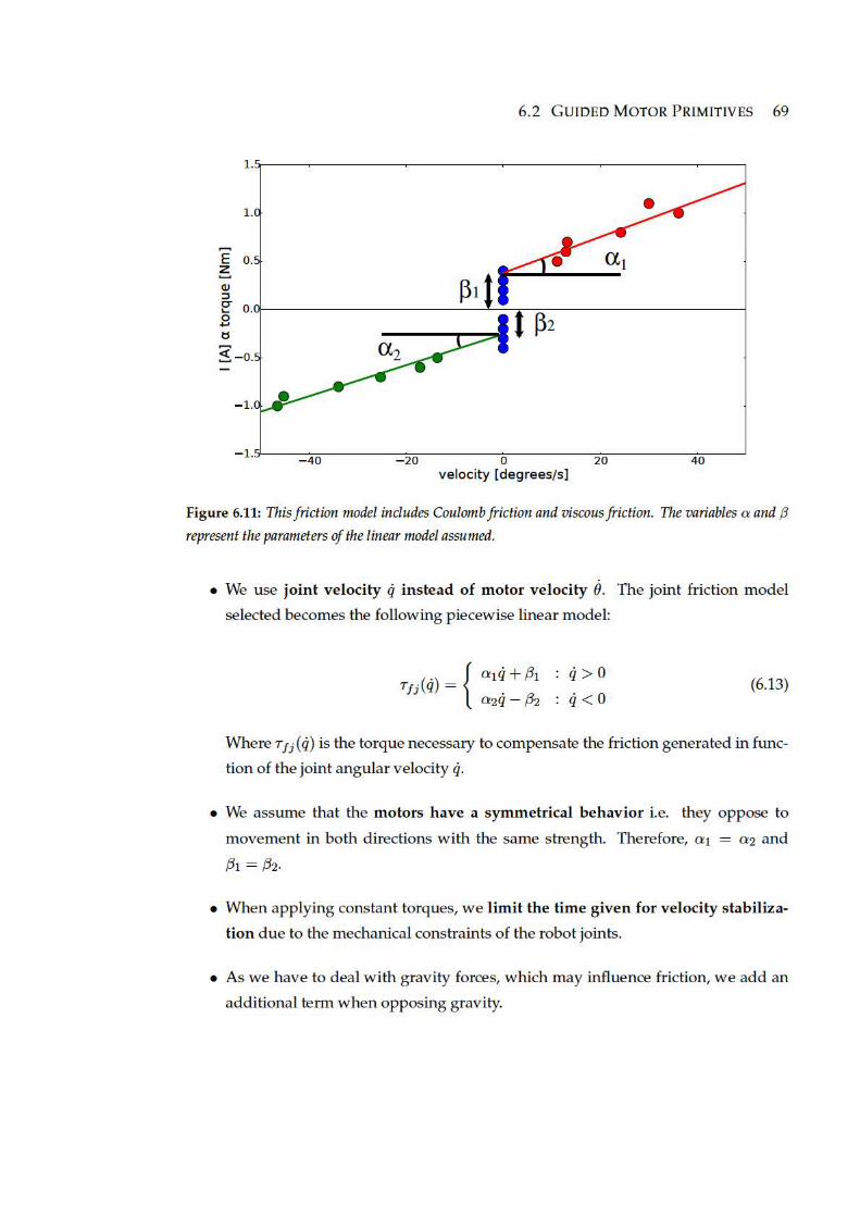

70 EXECUTION
Robot joints have mechanical constraints, so there is a limit in the time the joint
velocity can be recorded. This time may not be enough for the velocity to stabilize. In
these cases, the velocity achieved before reaching the joint limit must be used instead
of the stabilized velocity. This causes a steeper slope of the posterior linear regression.
The final parameters of the linear regression should be further adjusted in these cases.
As stated in our final assumption, we add a term in addition to τfj(q). We assume
that an additional mechanical friction is generated in the motor axle and gearbox due
to gravity. This is the reason why we have added a term τfg dependent on the joint
position and the velocity:
τfg = f(q, q) (6.14)
The term τfg(q, q) is purely experimental, as it depends on the mechanical design
and construction of the robot. In our model, we only add this term when the grav-
ity opposes the direction movement of the arm. To see whether the gravity is in favor
or against this movement, the variation of the potential energy U can be used. When
∆U > 0, the movement is against gravity. The final friction compensator can be ex-
pressed as:
τf (q, q) =
{τfj(q) + τfg(q, q) : ∆U > 0
τfj(q) : ∆U < 0(6.15)
Different applications may require different behaviors of the robot. Hence, two con-
trollers have been derived from the generic friction and gravity compensation controller
(6.4).
Low-Friction Zero-Gravity controller (LFZG) This controller can improve the physi-
cal interaction with robots. In this controller, a new parameter ξ has been incorporated.
This parameter attenuates the influence of the friction compensation on the system.
Introducing ξ in the controller, it becomes:
u = g(q) + ξτf (q, q) (6.16)
By setting 0 < ξ < 1, this controller allows the robot to move easily, without
effort, but eventually stopping due to the low friction. This controller can be use-
ful in paradigms such as keyframe demonstration and PbD, where there is a direct
6.2 GUIDED MOTOR PRIMITIVES 71
physical contact with the robot. For instance, when aiming to record a task using
keyframe demonstration, different robot configurations must be recorded. In many
cases, a demonstrator may have to use both hands to move a single robot joint, due to
its individual friction. Therefore, in robots with many DoF, it can be difficult to physi-
cally move the robot between the different desired configurations. Using our controller,
one has to simply push the robot in the desired direction, and stop it when desired. The
attenuated friction serves as an aid for stopping at the desired target keyframes.
Zero-Friction Zero-Gravity controller (ZFZG) This controller, when applied to all the
joints, ideally makes the robot move as if only the external dynamic forces and inertia
would modify the motion. To achieve this behavior, we can use the generic friction and
gravity compensation controller (6.4):
u = g(q) + τf (q, q) (6.17)
This controller, which is a special case of LFZG, can be useful for situations where it
is interesting to simulate gravity-free conditions. A robotic platform using this control
could be employed to test how devices would behave in complete absence of friction
and gravity. Obviously, this behavior would only be reached if the controller is able
to compensate perfectly both gravity and friction. Usually, such accuracy will not be
achieved, and the controller will behave as a LFZG with a ξ close to one.
The theoretical descriptions and the mathematical formulations of the research of
this thesis end with this chapter. The next chapters will focus on experimental valida-
tion, analysis of the results and their discussion.

72 EXECUTION
73
Chapter 7Experiments
Many different research topics and novel techniques have been presented in this
thesis. In this chapter, each novelty is analyzed in its own section.
1. Demonstration and feature selection is tested by recording several demonstra-
tions of a task using the robot’s sensor devices. This information is subject of
study. See Section 7.1.
2. CGDA recognition is evaluated. Despite recognition is implicitly evaluated in the
execution section, it is also tested independently. See Section 7.2.
3. CGDA using evolutionary computation is tested in a simulated scenario. Two
tasks objectives are evaluated, using all the evolutionary strategies presented be-
fore. See Section 7.3.
4. To create a Guided Motor Primitives library, a human has guided a humanoid
robot’s arm in random movements. The generated primitives are evaluated in a
simulated scenario. GMP and its tree search algorithm substitute evolutionary
computation, as optimization technique, in this experiment. See Section 7.4.
5. Finally, friction and gravity compensation is applied to 1 DoF of the robot arm to
test the effectiveness of the approach. See Section 7.5.
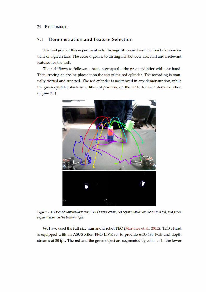
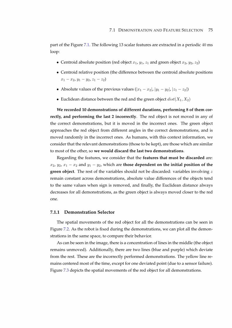
7.1 DEMONSTRATION AND FEATURE SELECTION 75
part of the Figure 7.1. The following 13 scalar features are extracted in a periodic 40 ms
loop:
• Centroid absolute position (red object x1, y1, z1 and green object x2, y2, z2)
• Centroid relative position (the difference between the centroid absolute positions
x1 − x2, y1 − y2, z1 − z2)
• Absolute values of the previous values (|x1 − x2|, |y1 − y2|, |z1 − z2|)
• Euclidean distance between the red and the green object dist(X1, X2)
We recorded 10 demonstrations of different durations, performing 8 of them cor-
rectly, and performing the last 2 incorrectly. The red object is not moved in any of
the correct demonstrations, but it is moved in the incorrect ones. The green object
approaches the red object from different angles in the correct demonstrations, and is
moved randomly in the incorrect ones. As humans, with this context information, we
consider that the relevant demonstrations (those to be kept), are those which are similar
to most of the other, so we would discard the last two demonstrations.
Regarding the features, we consider that the features that must be discarded are:
x2, y2, x1 − x2 and y1 − y2, which are those dependent on the initial position of the
green object. The rest of the variables should not be discarded: variables involving z
remain constant across demonstrations, absolute value differences of the objects tend
to the same values when sign is removed, and finally, the Euclidean distance always
decreases for all demonstrations, as the green object is always moved closer to the red
one.
7.1.1 Demonstration Selector
The spatial movements of the red object for all the demonstrations can be seen in
Figure 7.2. As the robot is fixed during the demonstrations, we can plot all the demon-
strations in the same space, to compare their behavior.
As can be seen in the image, there is a concentration of lines in the middle (the object
remains unmoved). Additionally, there are two lines (blue and purple) which deviate
from the rest. These are the incorrectly performed demonstrations. The yellow line re-
mains centered most of the time, except for one deviated point (due to a sensor failure).
Figure 7.3 depicts the spatial movements of the red object for all demonstrations.
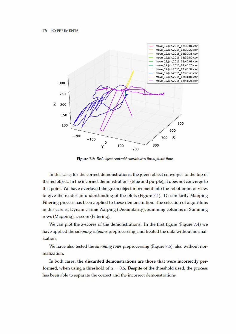
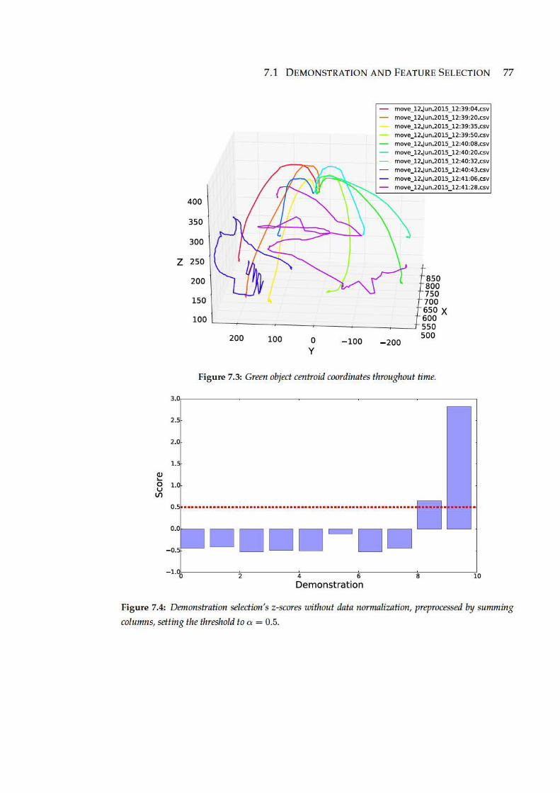
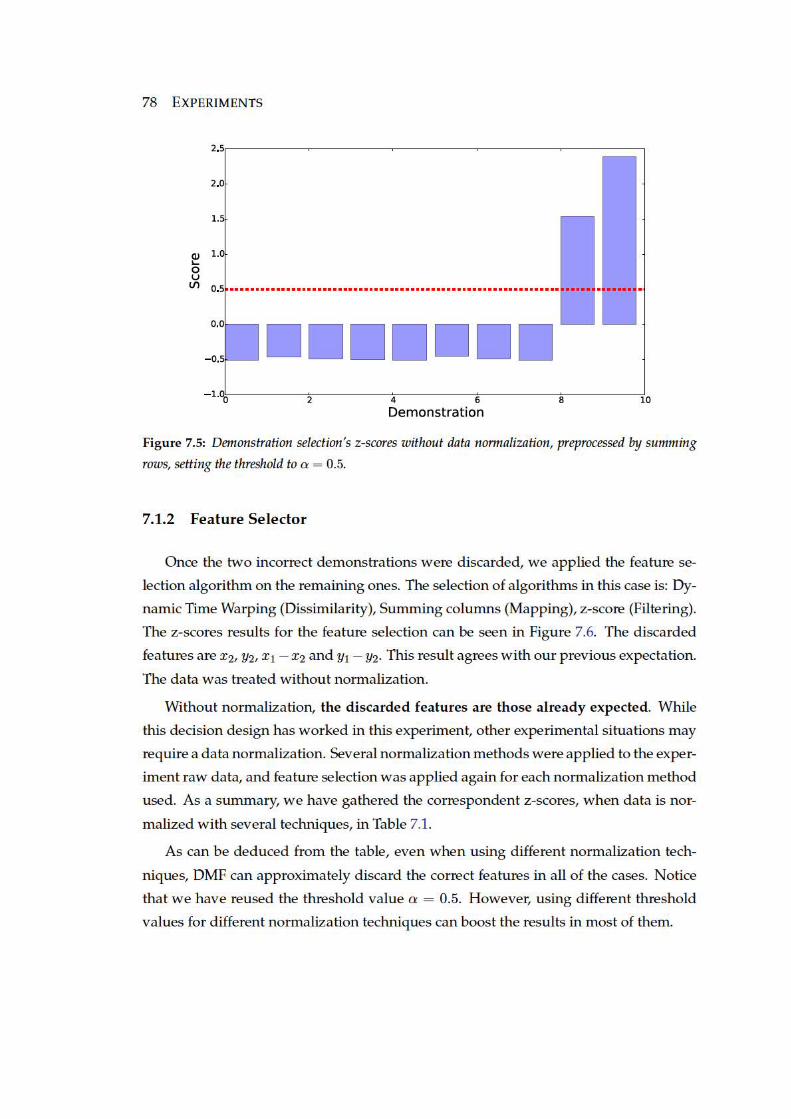
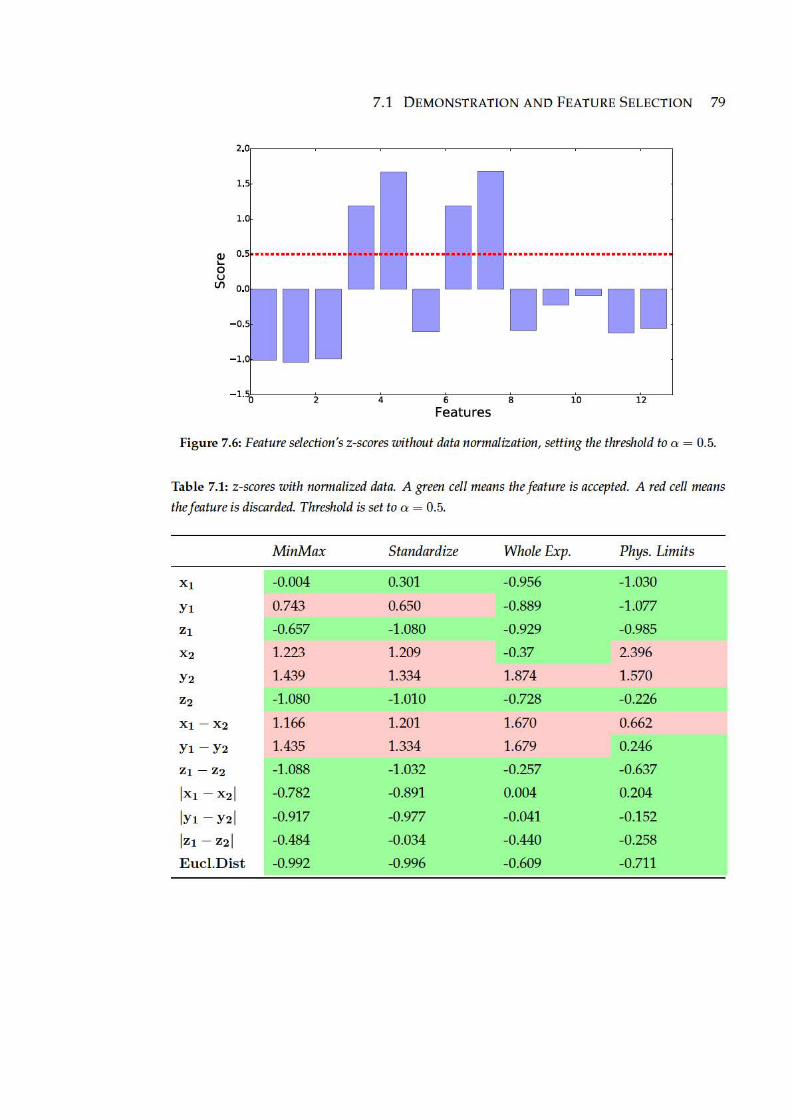

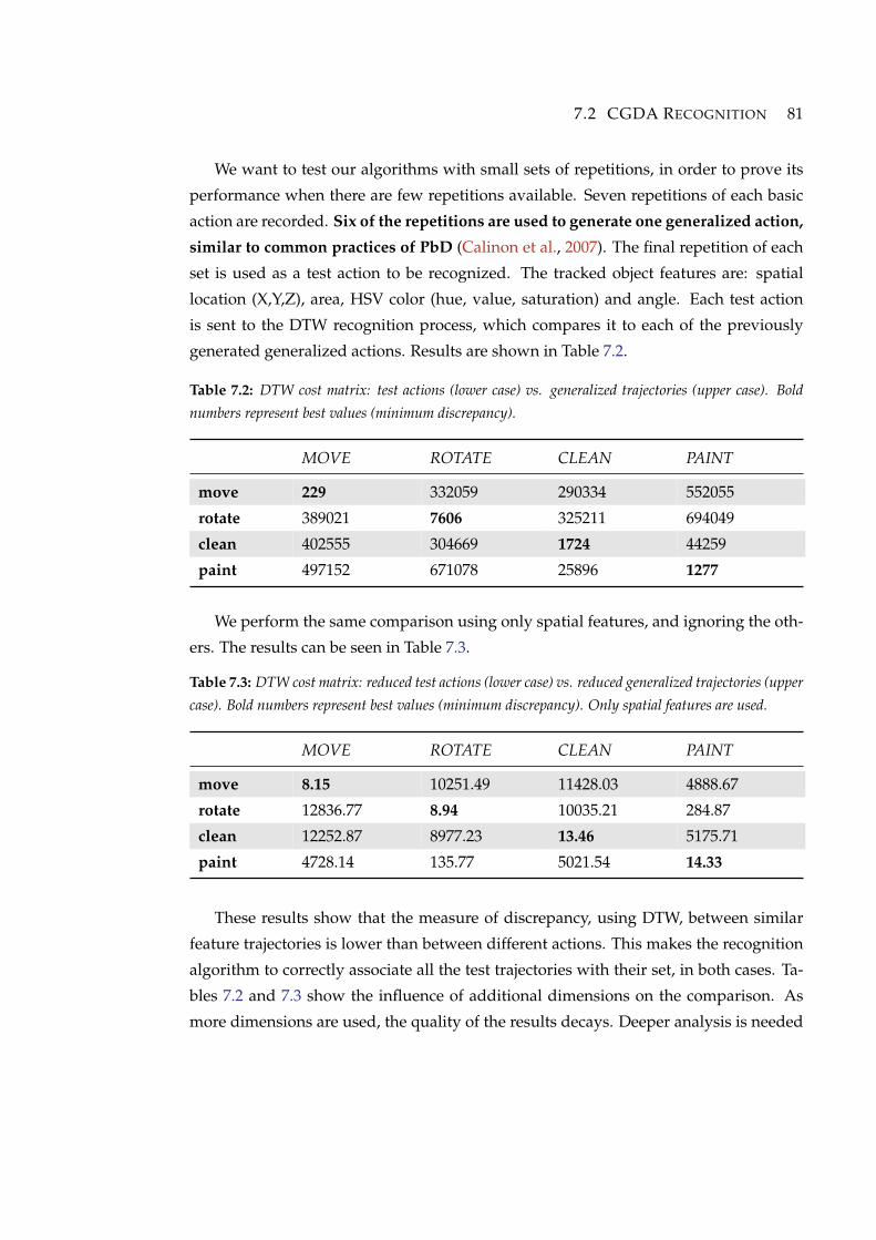
7.2 CGDA RECOGNITION 81
We want to test our algorithms with small sets of repetitions, in order to prove its
performance when there are few repetitions available. Seven repetitions of each basic
action are recorded. Six of the repetitions are used to generate one generalized action,
similar to common practices of PbD (Calinon et al., 2007). The final repetition of each
set is used as a test action to be recognized. The tracked object features are: spatial
location (X,Y,Z), area, HSV color (hue, value, saturation) and angle. Each test action
is sent to the DTW recognition process, which compares it to each of the previously
generated generalized actions. Results are shown in Table 7.2.
Table 7.2: DTW cost matrix: test actions (lower case) vs. generalized trajectories (upper case). Bold
numbers represent best values (minimum discrepancy).
MOVE ROTATE CLEAN PAINT
move 229 332059 290334 552055
rotate 389021 7606 325211 694049
clean 402555 304669 1724 44259
paint 497152 671078 25896 1277
We perform the same comparison using only spatial features, and ignoring the oth-
ers. The results can be seen in Table 7.3.
Table 7.3: DTW cost matrix: reduced test actions (lower case) vs. reduced generalized trajectories (upper
case). Bold numbers represent best values (minimum discrepancy). Only spatial features are used.
MOVE ROTATE CLEAN PAINT
move 8.15 10251.49 11428.03 4888.67
rotate 12836.77 8.94 10035.21 284.87
clean 12252.87 8977.23 13.46 5175.71
paint 4728.14 135.77 5021.54 14.33
These results show that the measure of discrepancy, using DTW, between similar
feature trajectories is lower than between different actions. This makes the recognition
algorithm to correctly associate all the test trajectories with their set, in both cases. Ta-
bles 7.2 and 7.3 show the influence of additional dimensions on the comparison. As
more dimensions are used, the quality of the results decays. Deeper analysis is needed
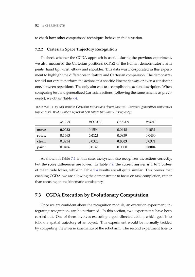
82 EXPERIMENTS
to check how other comparisons techniques behave in this situation.
7.2.2 Cartesian Space Trajectory Recognition
To check whether the CGDA approach is useful, during the previous experiment,
we also measured the Cartesian positions (X,Y,Z) of the human demonstrator’s arm
joints: hand tip, wrist, elbow and shoulder. This data was incorporated in this experi-
ment to highlight the differences in feature and Cartesian comparison. The demonstra-
tor did not care to perform the actions in a specific kinematic way, or even a consistent
one, between repetitions. The only aim was to accomplish the action description. When
comparing test and generalized Cartesian actions (following the same scheme as previ-
ously), we obtain Table 7.4.
Table 7.4: DTW cost matrix: Cartesian test actions (lower case) vs. Cartesian generalized trajectories
(upper case). Bold numbers represent best values (minimum discrepancy).
MOVE ROTATE CLEAN PAINT
move 0.0032 0.1594 0.0448 0.1031
rotate 0.1563 0.0123 0.0939 0.0430
clean 0.0234 0.0323 0.0003 0.0371
paint 0.0486 0.0148 0.0300 0.0004
As shown in Table 7.4, in this case, the system also recognizes the actions correctly,
but the score differences are lower. In Table 7.2, the correct answer is 1 to 3 orders
of magnitude lower, while in Table 7.4 results are all quite similar. This proves that
enabling CGDA, we are allowing the demonstrator to focus on task completion, rather
than focusing on the kinematic consistency.
7.3 CGDA Execution by Evolutionary Computation
Once we are confident about the recognition module, an execution experiment, in-
tegrating recognition, can be performed. In this section, two experiments have been
carried out. One of them involves executing a goal-directed action, which goal is to
follow a spatial trajectory of an object. This experiment would be normally tackled
by computing the inverse kinematics of the robot arm. The second experiment tries to
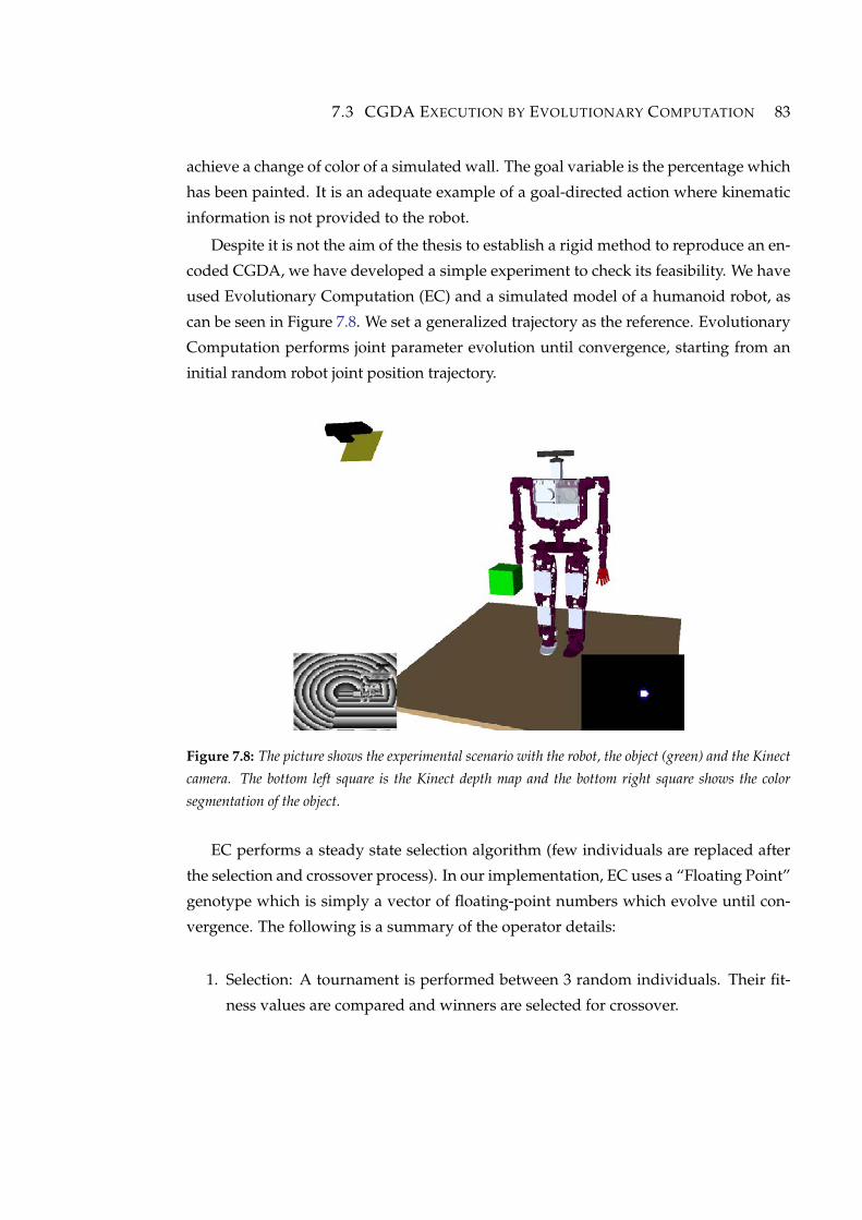
7.3 CGDA EXECUTION BY EVOLUTIONARY COMPUTATION 83
achieve a change of color of a simulated wall. The goal variable is the percentage which
has been painted. It is an adequate example of a goal-directed action where kinematic
information is not provided to the robot.
Despite it is not the aim of the thesis to establish a rigid method to reproduce an en-
coded CGDA, we have developed a simple experiment to check its feasibility. We have
used Evolutionary Computation (EC) and a simulated model of a humanoid robot, as
can be seen in Figure 7.8. We set a generalized trajectory as the reference. Evolutionary
Computation performs joint parameter evolution until convergence, starting from an
initial random robot joint position trajectory.
Figure 7.8: The picture shows the experimental scenario with the robot, the object (green) and the Kinect
camera. The bottom left square is the Kinect depth map and the bottom right square shows the color
segmentation of the object.
EC performs a steady state selection algorithm (few individuals are replaced after
the selection and crossover process). In our implementation, EC uses a “Floating Point”
genotype which is simply a vector of floating-point numbers which evolve until con-
vergence. The following is a summary of the operator details:
1. Selection: A tournament is performed between 3 random individuals. Their fit-
ness values are compared and winners are selected for crossover.
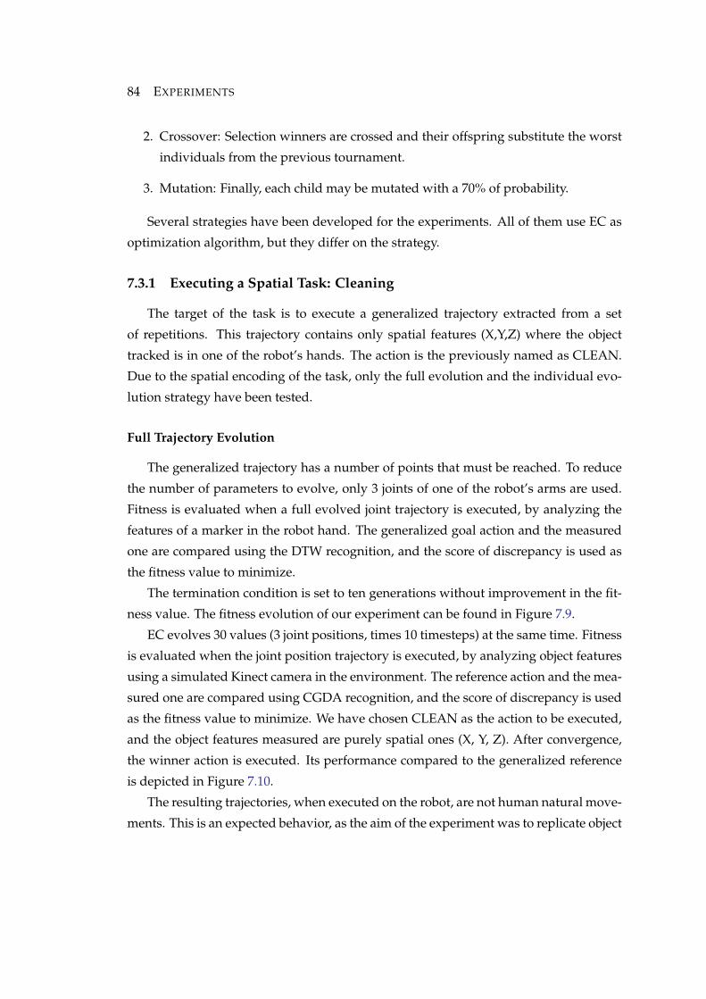
84 EXPERIMENTS
2. Crossover: Selection winners are crossed and their offspring substitute the worst
individuals from the previous tournament.
3. Mutation: Finally, each child may be mutated with a 70% of probability.
Several strategies have been developed for the experiments. All of them use EC as
optimization algorithm, but they differ on the strategy.
7.3.1 Executing a Spatial Task: Cleaning
The target of the task is to execute a generalized trajectory extracted from a set
of repetitions. This trajectory contains only spatial features (X,Y,Z) where the object
tracked is in one of the robot’s hands. The action is the previously named as CLEAN.
Due to the spatial encoding of the task, only the full evolution and the individual evo-
lution strategy have been tested.
Full Trajectory Evolution
The generalized trajectory has a number of points that must be reached. To reduce
the number of parameters to evolve, only 3 joints of one of the robot’s arms are used.
Fitness is evaluated when a full evolved joint trajectory is executed, by analyzing the
features of a marker in the robot hand. The generalized goal action and the measured
one are compared using the DTW recognition, and the score of discrepancy is used as
the fitness value to minimize.
The termination condition is set to ten generations without improvement in the fit-
ness value. The fitness evolution of our experiment can be found in Figure 7.9.
EC evolves 30 values (3 joint positions, times 10 timesteps) at the same time. Fitness
is evaluated when the joint position trajectory is executed, by analyzing object features
using a simulated Kinect camera in the environment. The reference action and the mea-
sured one are compared using CGDA recognition, and the score of discrepancy is used
as the fitness value to minimize. We have chosen CLEAN as the action to be executed,
and the object features measured are purely spatial ones (X, Y, Z). After convergence,
the winner action is executed. Its performance compared to the generalized reference
is depicted in Figure 7.10.
The resulting trajectories, when executed on the robot, are not human natural move-
ments. This is an expected behavior, as the aim of the experiment was to replicate object
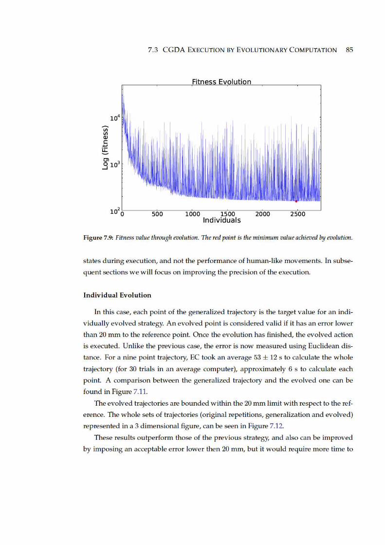
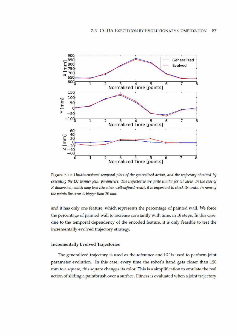
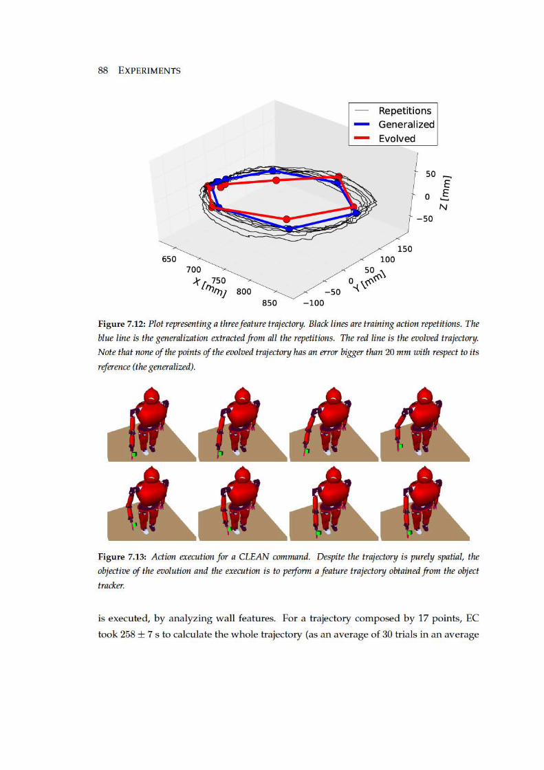

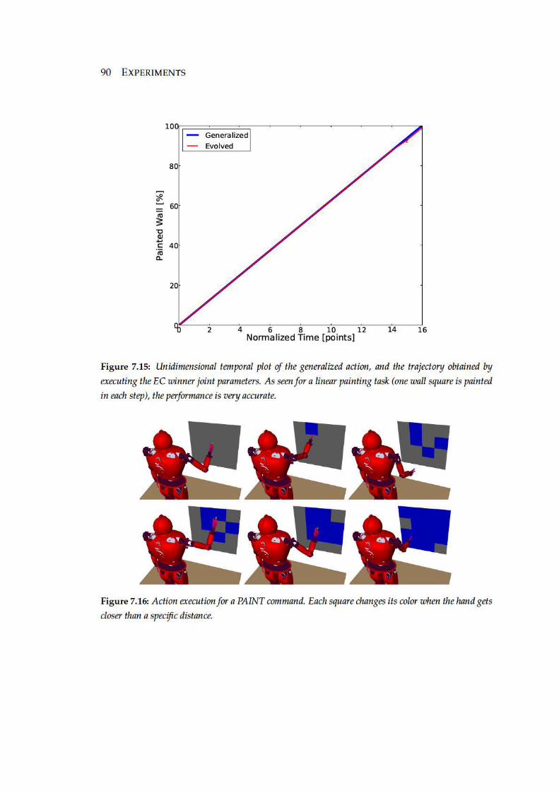
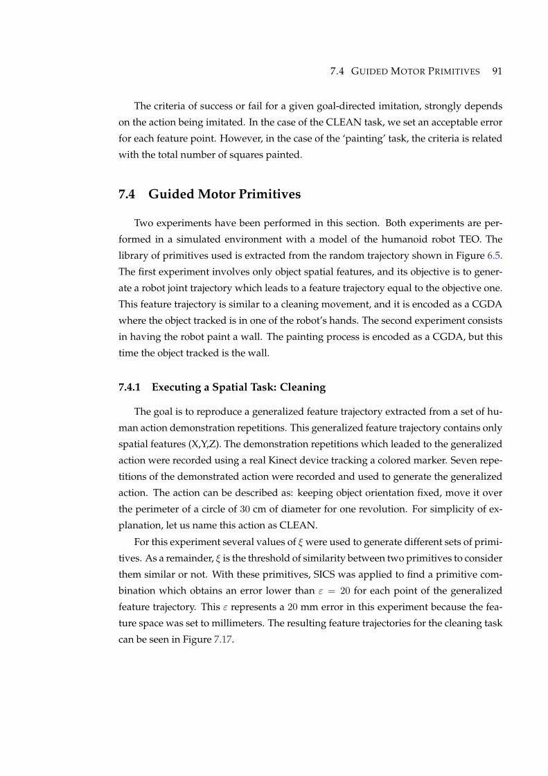
7.4 GUIDED MOTOR PRIMITIVES 91
The criteria of success or fail for a given goal-directed imitation, strongly depends
on the action being imitated. In the case of the CLEAN task, we set an acceptable error
for each feature point. However, in the case of the ‘painting’ task, the criteria is related
with the total number of squares painted.
7.4 Guided Motor Primitives
Two experiments have been performed in this section. Both experiments are per-
formed in a simulated environment with a model of the humanoid robot TEO. The
library of primitives used is extracted from the random trajectory shown in Figure 6.5.
The first experiment involves only object spatial features, and its objective is to gener-
ate a robot joint trajectory which leads to a feature trajectory equal to the objective one.
This feature trajectory is similar to a cleaning movement, and it is encoded as a CGDA
where the object tracked is in one of the robot’s hands. The second experiment consists
in having the robot paint a wall. The painting process is encoded as a CGDA, but this
time the object tracked is the wall.
7.4.1 Executing a Spatial Task: Cleaning
The goal is to reproduce a generalized feature trajectory extracted from a set of hu-
man action demonstration repetitions. This generalized feature trajectory contains only
spatial features (X,Y,Z). The demonstration repetitions which leaded to the generalized
action were recorded using a real Kinect device tracking a colored marker. Seven repe-
titions of the demonstrated action were recorded and used to generate the generalized
action. The action can be described as: keeping object orientation fixed, move it over
the perimeter of a circle of 30 cm of diameter for one revolution. For simplicity of ex-
planation, let us name this action as CLEAN.
For this experiment several values of ξ were used to generate different sets of primi-
tives. As a remainder, ξ is the threshold of similarity between two primitives to consider
them similar or not. With these primitives, SICS was applied to find a primitive com-
bination which obtains an error lower than ε = 20 for each point of the generalized
feature trajectory. This ε represents a 20 mm error in this experiment because the fea-
ture space was set to millimeters. The resulting feature trajectories for the cleaning task
can be seen in Figure 7.17.
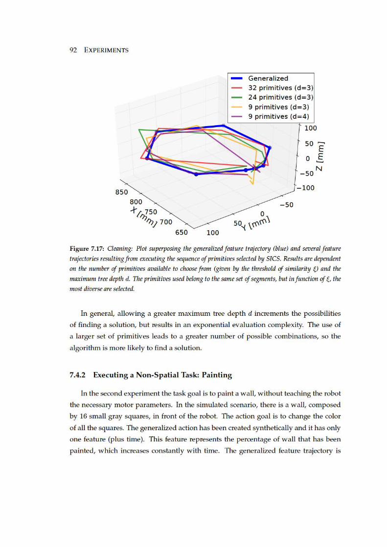
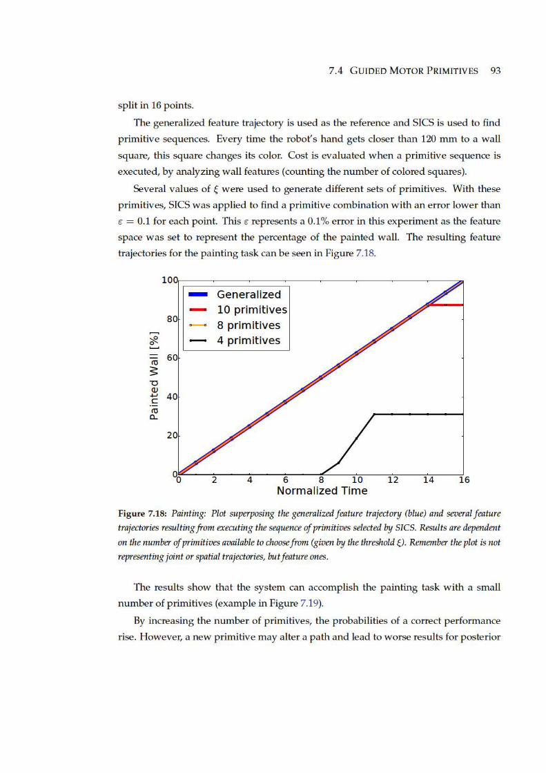
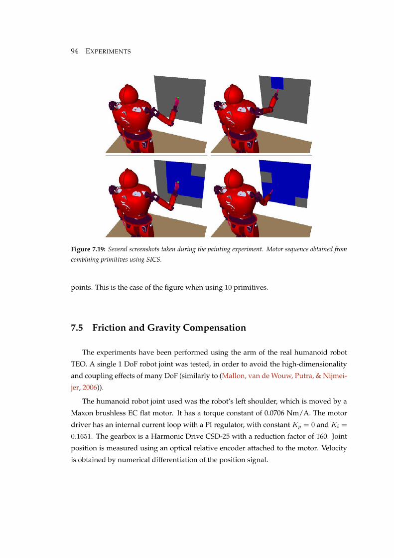
94 EXPERIMENTS
Figure 7.19: Several screenshots taken during the painting experiment. Motor sequence obtained from
combining primitives using SICS.
points. This is the case of the figure when using 10 primitives.
7.5 Friction and Gravity Compensation
The experiments have been performed using the arm of the real humanoid robot
TEO. A single 1 DoF robot joint was tested, in order to avoid the high-dimensionality
and coupling effects of many DoF (similarly to (Mallon, van de Wouw, Putra, & Nijmei-
jer, 2006)).
The humanoid robot joint used was the robot’s left shoulder, which is moved by a
Maxon brushless EC flat motor. It has a torque constant of 0.0706 Nm/A. The motor
driver has an internal current loop with a PI regulator, with constant Kp = 0 and Ki =
0.1651. The gearbox is a Harmonic Drive CSD-25 with a reduction factor of 160. Joint
position is measured using an optical relative encoder attached to the motor. Velocity
is obtained by numerical differentiation of the position signal.

7.5 FRICTION AND GRAVITY COMPENSATION 95
7.5.1 Computation
The robot arm weight m is 4.446 kg (including hand and electronics), and it has a
length L of 0.82 m. The gravity compensation term of the control was computed as the
torque caused by the arm modeled as a punctual mass at its center of gravity. Consid-
ering h as the height of the center of gravity with respect to its lowest position, being a
single joint, this term is trivial to be calculated. Assuming q1 as the angle between the
arm and the trunk, the potential energy of a mass situated at L/2 from the shoulder is:
U = mg0 h = mg0(L/2)(1− cos(q1)) (7.1)
Then, the gravity torque term is:
g(q1) =∂U
∂q1= mg0(L/2) sin(q1) (7.2)
The friction compensation term was determined by the procedure derived from
(Virgala & Kelemen, 2013), which leads to a model like the one in Equation (6.15). When
high torques are applied to the motor, leading to high velocities, the motor is not able
to stabilize its velocity before reaching the mechanical limit. This results in a steeper
slope on the posterior regression. This effect can be seen in the shortest curves in Figure
7.20. Fourteen different constant motor torques were tested, including both movements
against and in favor of gravity, ranging between −0.0706 Nm and 0.0706 Nm (ranging
from−1 A to 1 A). The robot’s arm is placed so that positive motor velocities go against
gravity, and negative velocities are in favor of gravity. To determine the friction term,
a summary of the process can be seen first in Figure 7.20, where the stability velocities
are measured, and then in Figure 7.21, which depicts the performed linear regressions.
The linear regressions obtained without manual tunning resulted in:
τf (q1) =
{0.009 q1 + 0.490 : ∆U > 0
0.005 q1 − 0.586 : ∆U < 0(7.3)
A manual adjustment of these linear regression parameters resulted in:
τf (q1) =
{0.006 q1 + 0.4 : ∆U > 0
0.001 q1 − 0.7 : ∆U < 0(7.4)
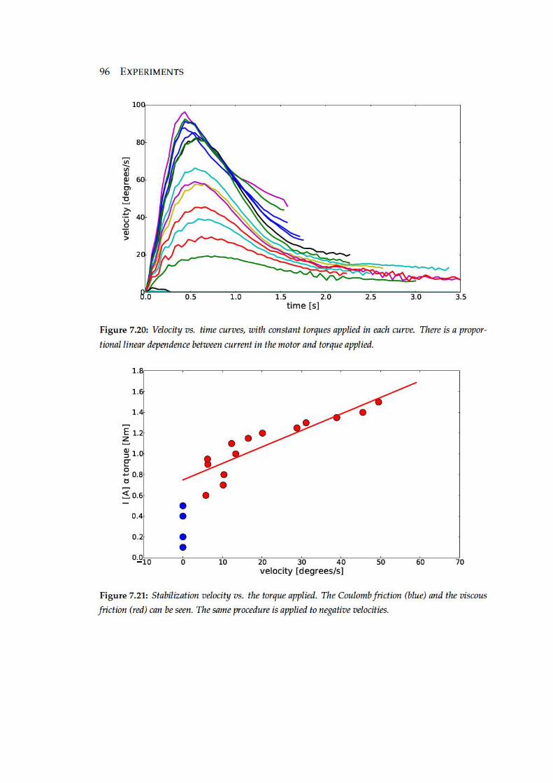
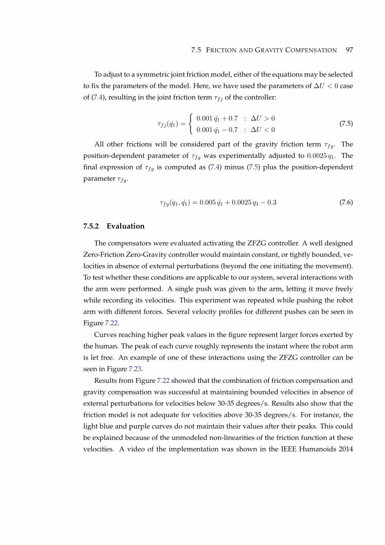
7.5 FRICTION AND GRAVITY COMPENSATION 97
To adjust to a symmetric joint friction model, either of the equations may be selected
to fix the parameters of the model. Here, we have used the parameters of ∆U < 0 case
of (7.4), resulting in the joint friction term τfj of the controller:
τfj(q1) =
{0.001 q1 + 0.7 : ∆U > 0
0.001 q1 − 0.7 : ∆U < 0(7.5)
All other frictions will be considered part of the gravity friction term τfg. The
position-dependent parameter of τfg was experimentally adjusted to 0.0025 q1. The
final expression of τfg is computed as (7.4) minus (7.5) plus the position-dependent
parameter τfg.
τfg(q1, q1) = 0.005 q1 + 0.0025 q1 − 0.3 (7.6)
7.5.2 Evaluation
The compensators were evaluated activating the ZFZG controller. A well designed
Zero-Friction Zero-Gravity controller would maintain constant, or tightly bounded, ve-
locities in absence of external perturbations (beyond the one initiating the movement).
To test whether these conditions are applicable to our system, several interactions with
the arm were performed. A single push was given to the arm, letting it move freely
while recording its velocities. This experiment was repeated while pushing the robot
arm with different forces. Several velocity profiles for different pushes can be seen in
Figure 7.22.
Curves reaching higher peak values in the figure represent larger forces exerted by
the human. The peak of each curve roughly represents the instant where the robot arm
is let free. An example of one of these interactions using the ZFZG controller can be
seen in Figure 7.23.
Results from Figure 7.22 showed that the combination of friction compensation and
gravity compensation was successful at maintaining bounded velocities in absence of
external perturbations for velocities below 30-35 degrees/s. Results also show that the
friction model is not adequate for velocities above 30-35 degrees/s. For instance, the
light blue and purple curves do not maintain their values after their peaks. This could
be explained because of the unmodeled non-linearities of the friction function at these
velocities. A video of the implementation was shown in the IEEE Humanoids 2014

99
Chapter 8Discussion and Conclussions
In this chapter, a discussion about each development introduced in this thesis is
presented. Conclusions and future works are also depicted at the end of the chapter.
8.1 Normalization on Demonstration and Feature Selection
In our demonstration and feature selection experiment, all the features were mea-
sured in the same distance units. This may not be case for other experiments, so data
normalization may be a requirement. While it may be necessary, normalization may
dangerously distort the data. The following is a description derived from of our own
experience upon using the different methods presented in Subsection 4.2.1.
• MinMax: When normalizing each feature within its empirical limits, the noise in
the signal may be amplified. For instance, a flat signal having sensor noise may
result in a signal where the noise has been greatly amplified.
• Standardized: Outliers may attenuate the signal. Imagine a sine wave signal
with a far outlier (e.g. a sensor failure). Having outliers often produces a signifi-
cant effect on the mean and standard deviation. When the signal is subtracted the
mean and divided by the standard deviation, it may be completely flattened.
• Whole Experiment Normalization: The data may be distorted by both of the
problems already explained.
100 DISCUSSION AND CONCLUSSIONS
• Physical Limits: This normalization implies that the designer has a previous
knowledge of each feature limit. In some cases, the limits will be imposed be
the sensor, while in other cases (e.g. derived features and combinations), math-
ematical limits must be determined. There is an additional issue when tasks do
not expand over the whole space because they are instead concentrated in a small
region, and features limits have been set with large ranges. When the signal is
normalized, it may be flattened, becoming no more relevant than noise.
It is an open discussion what technique is the most appropriate, and the authors
believe it will depend on the learning context.
8.2 Limitations of CGDA
We have used both Dynamic Time Warping and the Euclidean distance for recogni-
tion. Regarding the Euclidean distance results, there is a clear improvement in the error
between the trajectories, when comparing to DTW. However, a numerical comparison
would not be fair, e.g. comparing DTW to the distance error would be assuming that
the Euclidean distance is the “correct” metric. On its influence on execution, this change
forces the system to accomplish the feature variations in the correct order.
We have introduced an evolution strategy called Incrementally Evolved Trajecto-
ries (IET). This method has allowed us improve the performance of execution for non-
spatial features. IET shows an incremental time of computation for a sequence of points
until the valid space becomes very restricted. In these situations, we have observed
peaks in the computation time. Despite this fact, it allows experiments that were pre-
viously not feasible. The motor performance, in terms of velocities and acceleration, is
not taken into account. This thesis’ focus was on developing a feasible goal-directed
framework. Adapting this framework to work with real robots will imply a refine-
ment of the commanded motor signals, as well as determining the optimal number
of required human demonstrations.
Regarding the results obtained in the experimental section, we have demonstrated
that our CGDA approach is useful for execution even for non-spatial features. Thanks
to the use of the Euclidean distance, the trajectories can be evolved obtaining a high
degree of similarity, and this error is configurable for each evolution. Further analysis
need to be performed in order to assure that this method is applicable to other non-
8.3 THE BENEFITS OF HUMAN-ROBOT INTERACTION 101
spatial features. The biggest limitation of CGDA, is that execution, at this moment,
can only be performed in simulation. The techniques developed are not applicable to
the real world, as it is not feasible to perform thousands of iterations with a real robot.
8.3 The Benefits of Human-Robot Interaction
The inclusion of a human in the process of creation of Guided Motor Primitives
is very valuable. By benefiting from human-robot interaction, the complexity of the
framework is reduced when generating primitives.
Other self-discovery approaches, such as motor babbling, require programming
joint-limits and computing self-collisions. Despite GMP and motor babbling aim to
fill similar technological niches, our approach simplifies the process as it is the human
who leads the exploration of the joint space.
A limitation in our approach is that it is limited to simulation. As primitives are
combined and reproduced, collisions must be checked. This limits the applicability of
this approach to a real robot. A solution to this problem is to find the correct path in
simulation, and then transfer it to a real robot.
8.4 A More Accurate Compensation
The experiments of this set show, in general, an acceptable performance of the ZFZG
controller tested. More accurate friction models and identification procedures could
lead to improved controller behaviors under high joint velocity conditions, and would
also aid in maintaining the stability of low velocities. We also consider that using dif-
ferent dynamic robot models (pendulum-like models, or even the complete dynamic
model) may improve the results.
With the potential increase in complexity of the complete humanoid robot model, it
may be unavoidable to use machine learning algorithms which lighten the efforts nec-
essary to obtain a reliable friction and gravity compensation. They could also capture
the non-linearities present in the system.
These improvements may help at improving the general performance of the con-
troller. However for the use-case considered in this thesis, the controllers developed
are adequate, due to the low velocities of the interaction.
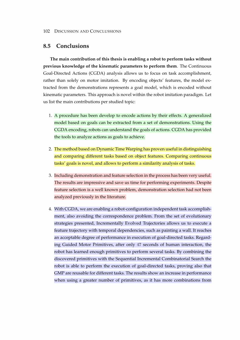
102 DISCUSSION AND CONCLUSSIONS
8.5 Conclusions
The main contribution of this thesis is enabling a robot to perform tasks without
previous knowledge of the kinematic parameters to perform them. The Continuous
Goal-Directed Actions (CGDA) analysis allows us to focus on task accomplishment,
rather than solely on motor imitation. By encoding objects’ features, the model ex-
tracted from the demonstrations represents a goal model, which is encoded without
kinematic parameters. This approach is novel within the robot imitation paradigm. Let
us list the main contributions per studied topic:
1. A procedure has been develop to encode actions by their effects. A generalized
model based on goals can be extracted from a set of demonstrations. Using the
CGDA encoding, robots can understand the goals of actions. CGDA has provided
the tools to analyze actions as goals to achieve.
2. The method based on Dynamic Time Warping has proven useful in distinguishing
and comparing different tasks based on object features. Comparing continuous
tasks’ goals is novel, and allows to perform a similarity analysis of tasks.
3. Including demonstration and feature selection in the process has been very useful.
The results are impressive and save us time for performing experiments. Despite
feature selection is a well known problem, demonstration selection had not been
analyzed previously in the literature.
4. With CGDA, we are enabling a robot-configuration independent task accomplish-
ment, also avoiding the correspondence problem. From the set of evolutionary
strategies presented, Incrementally Evolved Trajectories allows us to execute a
feature trajectory with temporal dependencies, such as painting a wall. It reaches
an acceptable degree of performance in execution of goal-directed tasks. Regard-
ing Guided Motor Primitives, after only 47 seconds of human interaction, the
robot has learned enough primitives to perform several tasks. By combining the
discovered primitives with the Sequential Incremental Combinatorial Search the
robot is able to perform the execution of goal-directed tasks, proving also that
GMP are reusable for different tasks. The results show an increase in performance
when using a greater number of primitives, as it has more combinations from
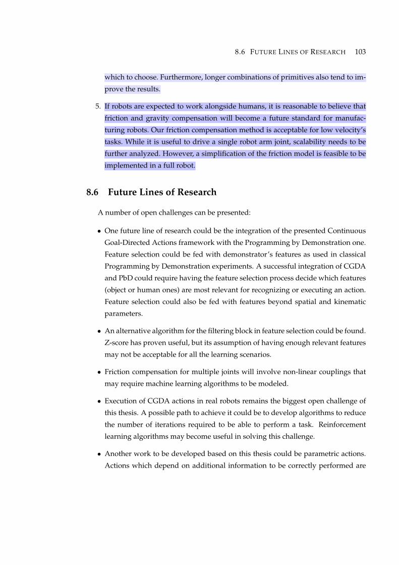
8.6 FUTURE LINES OF RESEARCH 103
which to choose. Furthermore, longer combinations of primitives also tend to im-
prove the results.
5. If robots are expected to work alongside humans, it is reasonable to believe that
friction and gravity compensation will become a future standard for manufac-
turing robots. Our friction compensation method is acceptable for low velocity’s
tasks. While it is useful to drive a single robot arm joint, scalability needs to be
further analyzed. However, a simplification of the friction model is feasible to be
implemented in a full robot.
8.6 Future Lines of Research
A number of open challenges can be presented:
• One future line of research could be the integration of the presented Continuous
Goal-Directed Actions framework with the Programming by Demonstration one.
Feature selection could be fed with demonstrator’s features as used in classical
Programming by Demonstration experiments. A successful integration of CGDA
and PbD could require having the feature selection process decide which features
(object or human ones) are most relevant for recognizing or executing an action.
Feature selection could also be fed with features beyond spatial and kinematic
parameters.
• An alternative algorithm for the filtering block in feature selection could be found.
Z-score has proven useful, but its assumption of having enough relevant features
may not be acceptable for all the learning scenarios.
• Friction compensation for multiple joints will involve non-linear couplings that
may require machine learning algorithms to be modeled.
• Execution of CGDA actions in real robots remains the biggest open challenge of
this thesis. A possible path to achieve it could be to develop algorithms to reduce
the number of iterations required to be able to perform a task. Reinforcement
learning algorithms may become useful in solving this challenge.
• Another work to be developed based on this thesis could be parametric actions.
Actions which depend on additional information to be correctly performed are
104 DISCUSSION AND CONCLUSSIONS
not taken into account at the current state of development. This is the case, for
instance, of the action paint: it is not the same to paint blue than to paint red. In
our feature space, these actions would end in different coordinates for the color
dimension. The solution to this problem could be to mix the structure here pre-
sented with semantic information, in a similar way to our previous work with
objects (Victores, Morante, Jardon, & Balaguer, 2013b).
With the advancements presented in this thesis, we are pioneering a new area of
research of robotics. Programming by Demonstration is a useful framework for current
robots, but future robots will evolve to satisfy new forms of interaction. Today we
must demonstrate each task to a robot, for it to mechanically repeat it. In the future,
robots should be able to reuse and combine previous experiences to perform new, or
even previously unseen, tasks. The author looks forward to seeing how the research
presented in this thesis may aid in this direction.

105
Appendices


107
Appendix AOpinion: Cryptobotics: Why robots
need cyber safety
With the expected introduction of robots into our daily lives, providing mechanisms
to avoid undesired attacks and exploits in robot communication software is becom-
ing increasingly required. Just as during the beginnings of the computer age (Pfleeger
& Pfleeger, 2002), robotics is established in a “happy naivety”, where security rules
against external attacks are not adopted, assuming that robotics knowledgeable peo-
ple are well intended. While this may have been true in the past, the mass adoption
of robots will increase the possibilities of attacks. This fact is specially relevant in de-
fense, medical and other critical fields involving humans, where tampering can result in
serious bodily harm and/or privacy invasions. For these reasons, we consider that re-
searchers and industry should deploy efforts in cyber safety and acquire good practices
when developing and distributing robot software. We propose the term Cryptobotics as
a unifying term for research and applications of computer and microcontrollers security
measures in robotics.
A.1 Stating The Problem
The problems that the field of robotics will face are similar to those the computer
revolution faced with the widespread of the Internet 30 years ago. Among the common
attacks computers may suffer, there are: denial-of-service, eavesdropping, spoofing,
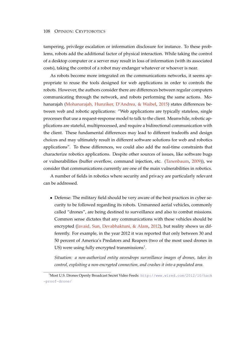
108 OPINION: CRYPTOBOTICS
tampering, privilege escalation or information disclosure for instance. To these prob-
lems, robots add the additional factor of physical interaction. While taking the control
of a desktop computer or a server may result in loss of information (with its associated
costs), taking the control of a robot may endanger whatever or whoever is near.
As robots become more integrated on the communications networks, it seems ap-
propriate to reuse the tools designed for web applications in order to controls the
robots. However, the authors consider there are differences between regular computers
communicating through the network, and robots performing the same actions. Mo-
hanarajah (Mohanarajah, Hunziker, D’Andrea, & Waibel, 2015) states differences be-
tween web and robotic applications: ”Web applications are typically stateless, single
processes that use a request-response model to talk to the client. Meanwhile, robotic ap-
plications are stateful, multiprocessed, and require a bidirectional communication with
the client. These fundamental differences may lead to different tradeoffs and design
choices and may ultimately result in different software solutions for web and robotics
applications”. To these differences, we could also add the real-time constraints that
characterize robotics applications. Despite other sources of issues, like software bugs
or vulnerabilities (buffer overflow, command injection, etc. (Tanenbaum, 2009)), we
consider that communications currently are one of the main vulnerabilities in robotics.
A number of fields in robotics where security and privacy are particularly relevant
can be addressed.
• Defense: The military field should be very aware of the best practices in cyber se-
curity to be followed regarding its robots. Unmanned aerial vehicles, commonly
called “drones”, are being destined to surveillance and also to combat missions.
Common sense dictates that any communications with these vehicles should be
encrypted (Javaid, Sun, Devabhaktuni, & Alam, 2012), but reality shows us dif-
ferently. For example, in the year 2012 it was reported that only between 30 and
50 percent of America’s Predators and Reapers (two of the most used drones in
US) were using fully encrypted transmissions1.
Situation: a non-authorized entity eavesdrops surveillance images of drones, takes its
control, exploiting a non-encrypted connection, and crashes it into a populated area.
1Most U.S. Drones Openly Broadcast Secret Video Feeds: http://www.wired.com/2012/10/hack
-proof-drone/
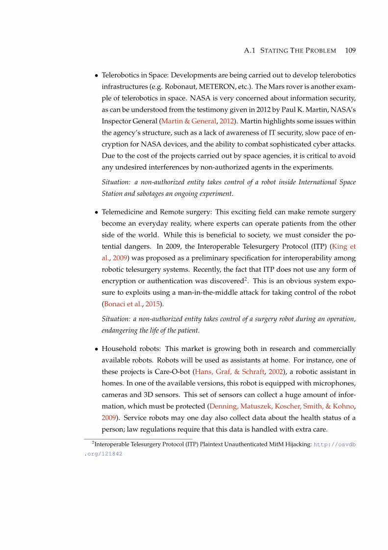
A.1 STATING THE PROBLEM 109
• Telerobotics in Space: Developments are being carried out to develop telerobotics
infrastructures (e.g. Robonaut, METERON, etc.). The Mars rover is another exam-
ple of telerobotics in space. NASA is very concerned about information security,
as can be understood from the testimony given in 2012 by Paul K. Martin, NASA’s
Inspector General (Martin & General, 2012). Martin highlights some issues within
the agency’s structure, such as a lack of awareness of IT security, slow pace of en-
cryption for NASA devices, and the ability to combat sophisticated cyber attacks.
Due to the cost of the projects carried out by space agencies, it is critical to avoid
any undesired interferences by non-authorized agents in the experiments.
Situation: a non-authorized entity takes control of a robot inside International Space
Station and sabotages an ongoing experiment.
• Telemedicine and Remote surgery: This exciting field can make remote surgery
become an everyday reality, where experts can operate patients from the other
side of the world. While this is beneficial to society, we must consider the po-
tential dangers. In 2009, the Interoperable Telesurgery Protocol (ITP) (King et
al., 2009) was proposed as a preliminary specification for interoperability among
robotic telesurgery systems. Recently, the fact that ITP does not use any form of
encryption or authentication was discovered2. This is an obvious system expo-
sure to exploits using a man-in-the-middle attack for taking control of the robot
(Bonaci et al., 2015).
Situation: a non-authorized entity takes control of a surgery robot during an operation,
endangering the life of the patient.
• Household robots: This market is growing both in research and commercially
available robots. Robots will be used as assistants at home. For instance, one of
these projects is Care-O-bot (Hans, Graf, & Schraft, 2002), a robotic assistant in
homes. In one of the available versions, this robot is equipped with microphones,
cameras and 3D sensors. This set of sensors can collect a huge amount of infor-
mation, which must be protected (Denning, Matuszek, Koscher, Smith, & Kohno,
2009). Service robots may one day also collect data about the health status of a
person; law regulations require that this data is handled with extra care.
2Interoperable Telesurgery Protocol (ITP) Plaintext Unauthenticated MitM Hijacking: http://osvdb
.org/121842
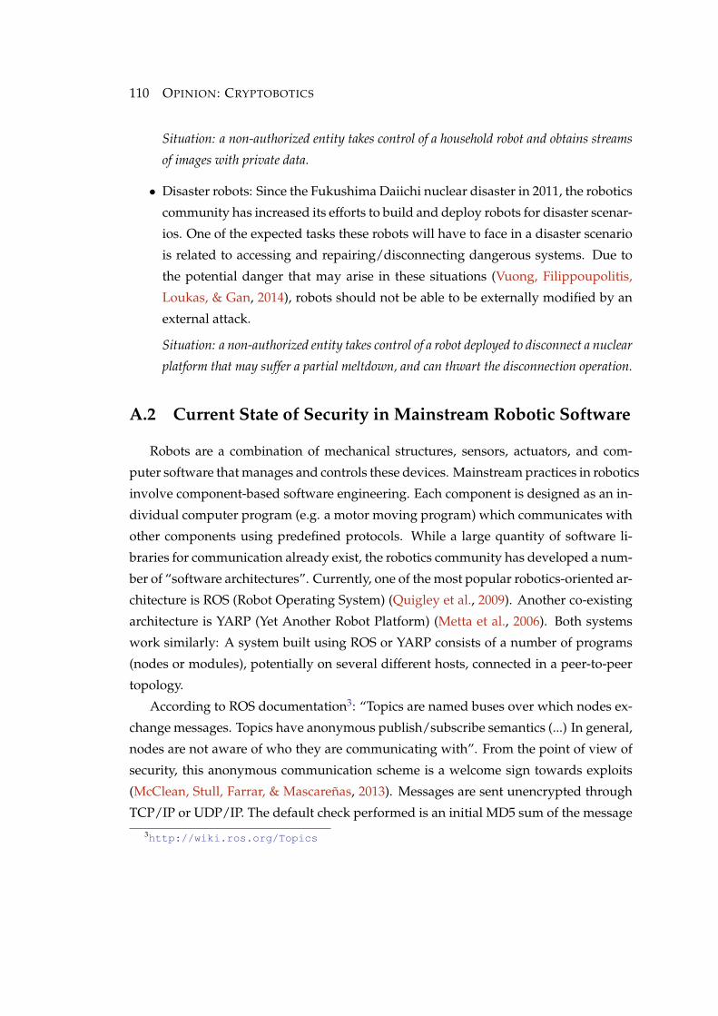
110 OPINION: CRYPTOBOTICS
Situation: a non-authorized entity takes control of a household robot and obtains streams
of images with private data.
• Disaster robots: Since the Fukushima Daiichi nuclear disaster in 2011, the robotics
community has increased its efforts to build and deploy robots for disaster scenar-
ios. One of the expected tasks these robots will have to face in a disaster scenario
is related to accessing and repairing/disconnecting dangerous systems. Due to
the potential danger that may arise in these situations (Vuong, Filippoupolitis,
Loukas, & Gan, 2014), robots should not be able to be externally modified by an
external attack.
Situation: a non-authorized entity takes control of a robot deployed to disconnect a nuclear
platform that may suffer a partial meltdown, and can thwart the disconnection operation.
A.2 Current State of Security in Mainstream Robotic Software
Robots are a combination of mechanical structures, sensors, actuators, and com-
puter software that manages and controls these devices. Mainstream practices in robotics
involve component-based software engineering. Each component is designed as an in-
dividual computer program (e.g. a motor moving program) which communicates with
other components using predefined protocols. While a large quantity of software li-
braries for communication already exist, the robotics community has developed a num-
ber of “software architectures”. Currently, one of the most popular robotics-oriented ar-
chitecture is ROS (Robot Operating System) (Quigley et al., 2009). Another co-existing
architecture is YARP (Yet Another Robot Platform) (Metta et al., 2006). Both systems
work similarly: A system built using ROS or YARP consists of a number of programs
(nodes or modules), potentially on several different hosts, connected in a peer-to-peer
topology.
According to ROS documentation3: “Topics are named buses over which nodes ex-
change messages. Topics have anonymous publish/subscribe semantics (...) In general,
nodes are not aware of who they are communicating with”. From the point of view of
security, this anonymous communication scheme is a welcome sign towards exploits
(McClean, Stull, Farrar, & Mascarenas, 2013). Messages are sent unencrypted through
TCP/IP or UDP/IP. The default check performed is an initial MD5 sum of the message3http://wiki.ros.org/Topics
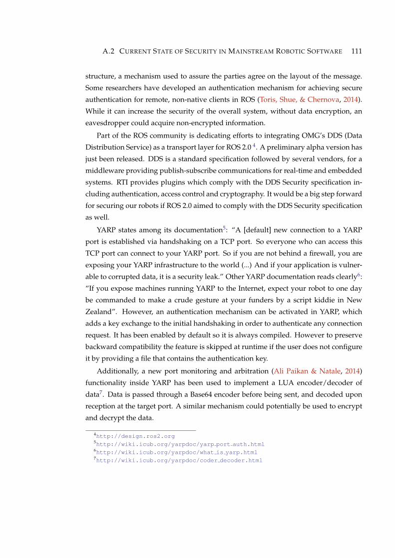
A.2 CURRENT STATE OF SECURITY IN MAINSTREAM ROBOTIC SOFTWARE 111
structure, a mechanism used to assure the parties agree on the layout of the message.
Some researchers have developed an authentication mechanism for achieving secure
authentication for remote, non-native clients in ROS (Toris, Shue, & Chernova, 2014).
While it can increase the security of the overall system, without data encryption, an
eavesdropper could acquire non-encrypted information.
Part of the ROS community is dedicating efforts to integrating OMG’s DDS (Data
Distribution Service) as a transport layer for ROS 2.0 4. A preliminary alpha version has
just been released. DDS is a standard specification followed by several vendors, for a
middleware providing publish-subscribe communications for real-time and embedded
systems. RTI provides plugins which comply with the DDS Security specification in-
cluding authentication, access control and cryptography. It would be a big step forward
for securing our robots if ROS 2.0 aimed to comply with the DDS Security specification
as well.
YARP states among its documentation5: “A [default] new connection to a YARP
port is established via handshaking on a TCP port. So everyone who can access this
TCP port can connect to your YARP port. So if you are not behind a firewall, you are
exposing your YARP infrastructure to the world (...) And if your application is vulner-
able to corrupted data, it is a security leak.” Other YARP documentation reads clearly6:
“If you expose machines running YARP to the Internet, expect your robot to one day
be commanded to make a crude gesture at your funders by a script kiddie in New
Zealand”. However, an authentication mechanism can be activated in YARP, which
adds a key exchange to the initial handshaking in order to authenticate any connection
request. It has been enabled by default so it is always compiled. However to preserve
backward compatibility the feature is skipped at runtime if the user does not configure
it by providing a file that contains the authentication key.
Additionally, a new port monitoring and arbitration (Ali Paikan & Natale, 2014)
functionality inside YARP has been used to implement a LUA encoder/decoder of
data7. Data is passed through a Base64 encoder before being sent, and decoded upon
reception at the target port. A similar mechanism could potentially be used to encrypt
and decrypt the data.
4http://design.ros2.org5http://wiki.icub.org/yarpdoc/yarp port auth.html6http://wiki.icub.org/yarpdoc/what is yarp.html7http://wiki.icub.org/yarpdoc/coder decoder.html
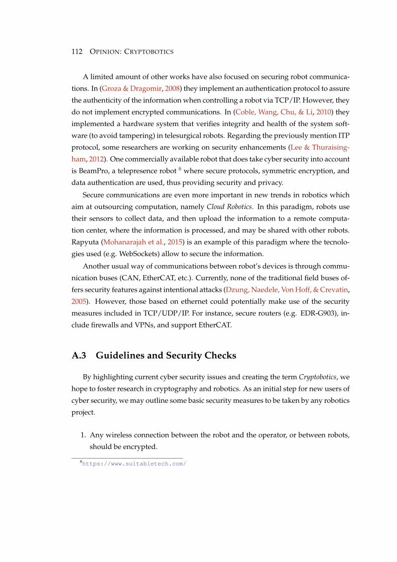
112 OPINION: CRYPTOBOTICS
A limited amount of other works have also focused on securing robot communica-
tions. In (Groza & Dragomir, 2008) they implement an authentication protocol to assure
the authenticity of the information when controlling a robot via TCP/IP. However, they
do not implement encrypted communications. In (Coble, Wang, Chu, & Li, 2010) they
implemented a hardware system that verifies integrity and health of the system soft-
ware (to avoid tampering) in telesurgical robots. Regarding the previously mention ITP
protocol, some researchers are working on security enhancements (Lee & Thuraising-
ham, 2012). One commercially available robot that does take cyber security into account
is BeamPro, a telepresence robot 8 where secure protocols, symmetric encryption, and
data authentication are used, thus providing security and privacy.
Secure communications are even more important in new trends in robotics which
aim at outsourcing computation, namely Cloud Robotics. In this paradigm, robots use
their sensors to collect data, and then upload the information to a remote computa-
tion center, where the information is processed, and may be shared with other robots.
Rapyuta (Mohanarajah et al., 2015) is an example of this paradigm where the tecnolo-
gies used (e.g. WebSockets) allow to secure the information.
Another usual way of communications between robot’s devices is through commu-
nication buses (CAN, EtherCAT, etc.). Currently, none of the traditional field buses of-
fers security features against intentional attacks (Dzung, Naedele, Von Hoff, & Crevatin,
2005). However, those based on ethernet could potentially make use of the security
measures included in TCP/UDP/IP. For instance, secure routers (e.g. EDR-G903), in-
clude firewalls and VPNs, and support EtherCAT.
A.3 Guidelines and Security Checks
By highlighting current cyber security issues and creating the term Cryptobotics, we
hope to foster research in cryptography and robotics. As an initial step for new users of
cyber security, we may outline some basic security measures to be taken by any robotics
project.
1. Any wireless connection between the robot and the operator, or between robots,
should be encrypted.
8https://www.suitabletech.com/
A.3 GUIDELINES AND SECURITY CHECKS 113
2. Always assume the environment is hostile when establishing communications.
Be sure that eavesdroppers cannot perform a man-in-the-middle attack by estab-
lishing key negotiation for insecure channels.
3. Any communication module (either a robot, a robot part, an operator, etc.) should
have a unique identifier, and each transmission should be able to be verified at
any moment to confirm the parties’ identities.
4. Any device is password protected, and its content encrypted.
5. When a high risk of message interception exists, communications should be im-
plemented following a perfect forward secrecy framework, where each commu-
nications is encrypted with a different key, assuring no previous (or future) com-
munication can be revealed if one key is discovered.
6. Access logs exist and are updated with each transmission. This may not prevent
an attack, but helps track where an attack came from. These files should be en-
crypted and should not be accessible with standard user privileges. A separate
password must protect them.
7. A firewall shielding access to internal communications should exist.
8. A place where passwords, keys and a registry of allowed users are stored should
exist. This place is the most critical device, and must be protected adequately.
An optional but strongly recommended requirement is to use audit and reviewed
open-source encryption software. Many public and well tested algorithms to encrypt
communication exist. Whenever possible, use largely accepted and community-checked
algorithms.
In terms of selection among algorithms, there are mainly three components in a
cyber security protocol: a public-key cryptosystem, used to derive symmetric-keys
(also called private-keys) which ensure confidentiality of data (Gupta, Gupta, Chang, &
Stebila, 2002), and a message authentication code (MAC) used to authenticate the data.
While this selection is a design decision open to system architects, the SSL protocol
recommends a cipher suite (combinations of algorithms) composed by RSA-RC4-SHA:
RSA as the public key, RC4 as the symmetric key, and SHA as a hash MAC.

114 OPINION: CRYPTOBOTICS
A.4 Discussion
A big market of opportunities for research regarding cyber safety in robotics exists.
Most robots are not yet prepared, from a security point of view, to be deployed in daily
life. The software is not prepared to protect against attacks, because communications
are usually unencrypted.
Regarding the dates of the exploits presented, and the current hype in deployment
of daily robotics (vacuum cleaners, amateur drones, etc.), Cryptobotics, understood as
a mix of cyber security and robotics, comes just in time to prepare these systems to be
safely used.
An important issue to be discussed is whether the implementation of encrypted
communications may affect the performance, specially in real-time systems. The ques-
tion about performance is highly dependant on the hardware, the software and the
network used. Encrypted communications on the Internet (https, ssh) show us that it
is possible to perform secure communications and offer remote services. For instance,
Adam Langley (Google Senior Software Engineer) has stated: ”when Google changed
Gmail from http to https (...) we had to deploy no additional machines and no special
hardware. On our production front-end machines, SSL/TLS accounts for less than 1
of the CPU load.”9. From our experience in humanoid robotics, a 1% overhead (while
respecting determinism in time) can be acceptable if it means our devices can be less
vulnerable to cyber attacks. Could an 8 MHz microcontroller perform real-time en-
cryption? Is it reasonable to implement authentication mechanisms along field buses
in time-constrained scenarios? This article intends to raise awareness for developers
to determine whether it is viable to integrate these mechanisms depending on each
specific use case.
Some people may ask why these problems have not been addressed previously. In
recent years, intrinsically safe industrial robots, the rise of domestic robots, and the use
of mobile robots in public spaces, have arisen issues that the robotics community did
not have to face in its previous 60 years of existence. Researchers are now focused on
developing applications to make robots useful, which may have made cyber safety a
low priority.
9https://www.imperialviolet.org/2010/06/25/overclocking-ssl.html
115
Appendix BTEO, The Humanoid Robot
In this appendix, we provide technical information about the humanoid robot TEO.
Simulated models have been constructed following these data.
• Axes and directions of rotation are shown in Figure B.1.
• Denavit-Hartenberg directions are shown in Figure B.2.
• Denavit-Hartenberg parameters are shown in Figure B.3.
• CAN (Controller Area Network) identification number of the joints are shown in
Figure B.4.
• YARP identification number of the joints are shown in Figure B.5.
• Mechanical links lengths distribution are shown in Figure B.6.
• Mechanical links lengths measurements are shown in Figure B.7.
• Position of the Center of Masses in the concentrated mass model are shown in
Figure B.8.

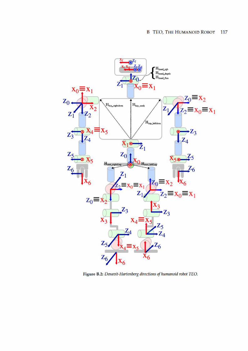
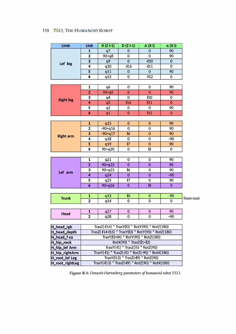
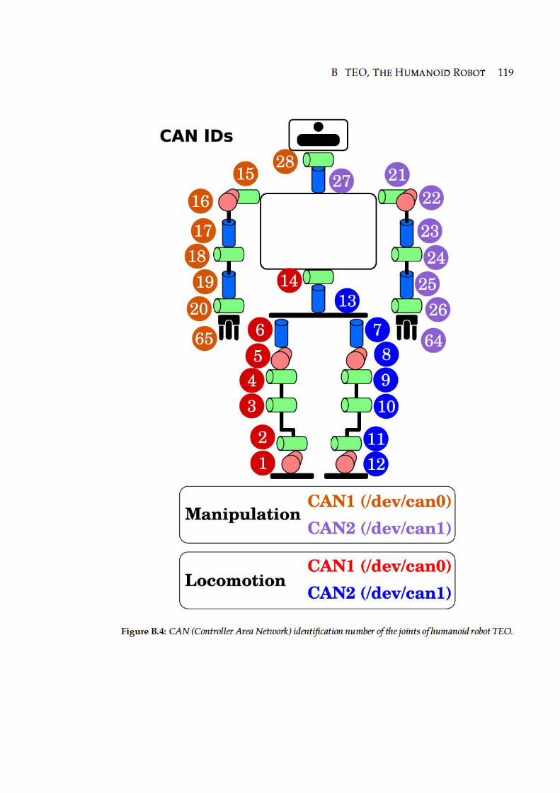
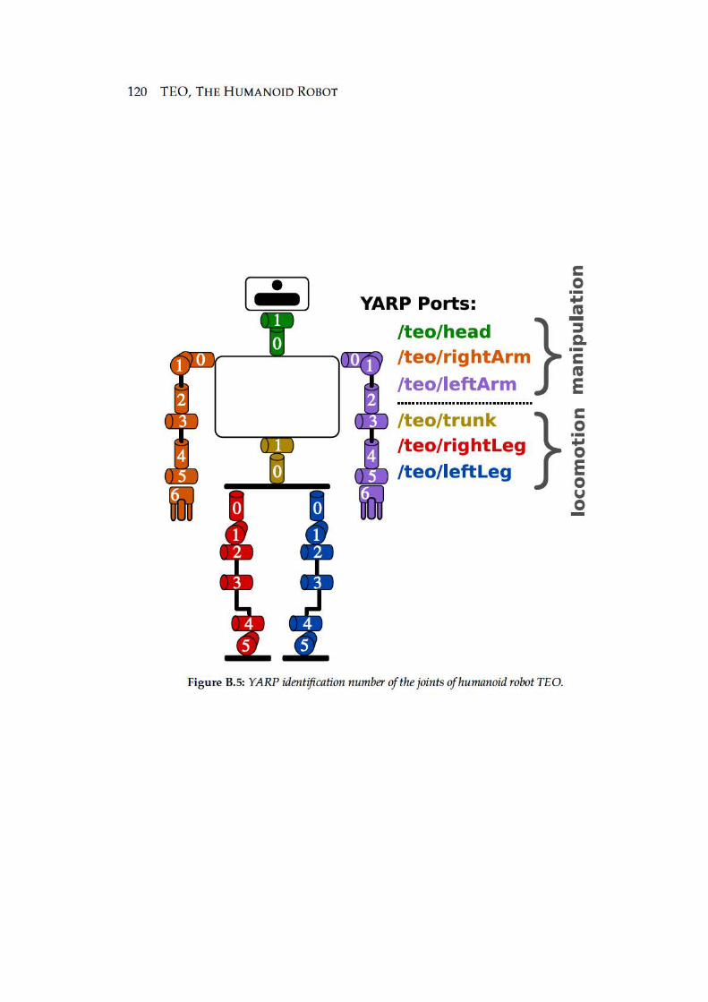
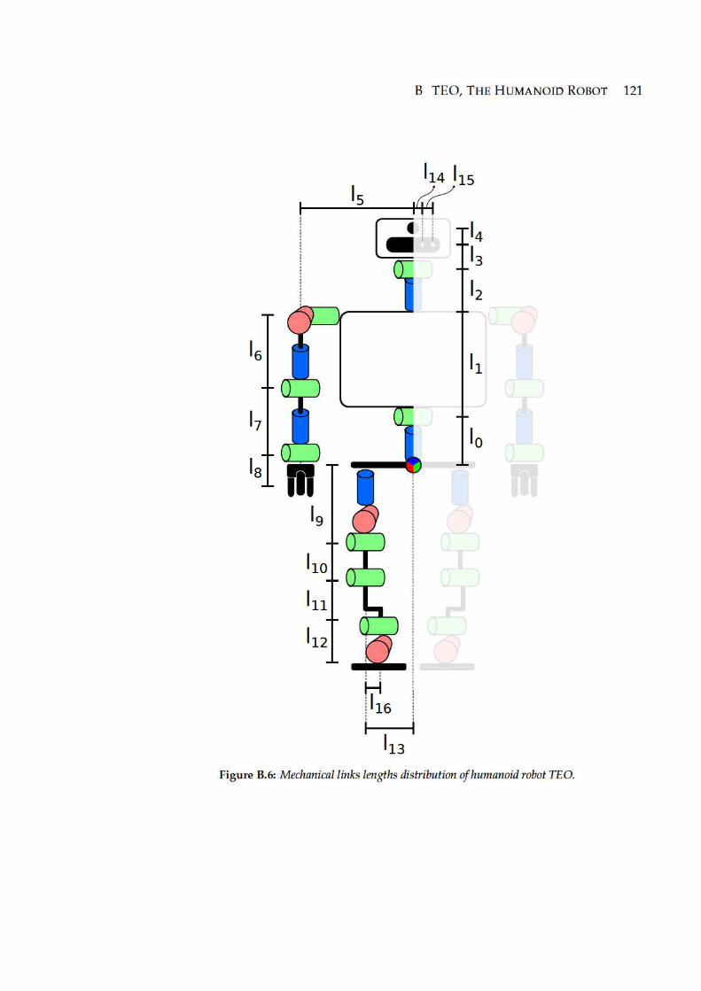
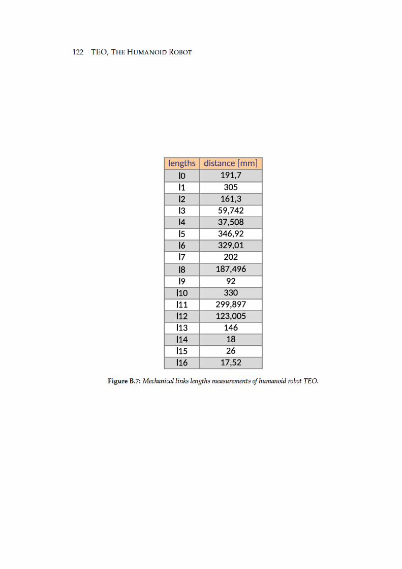
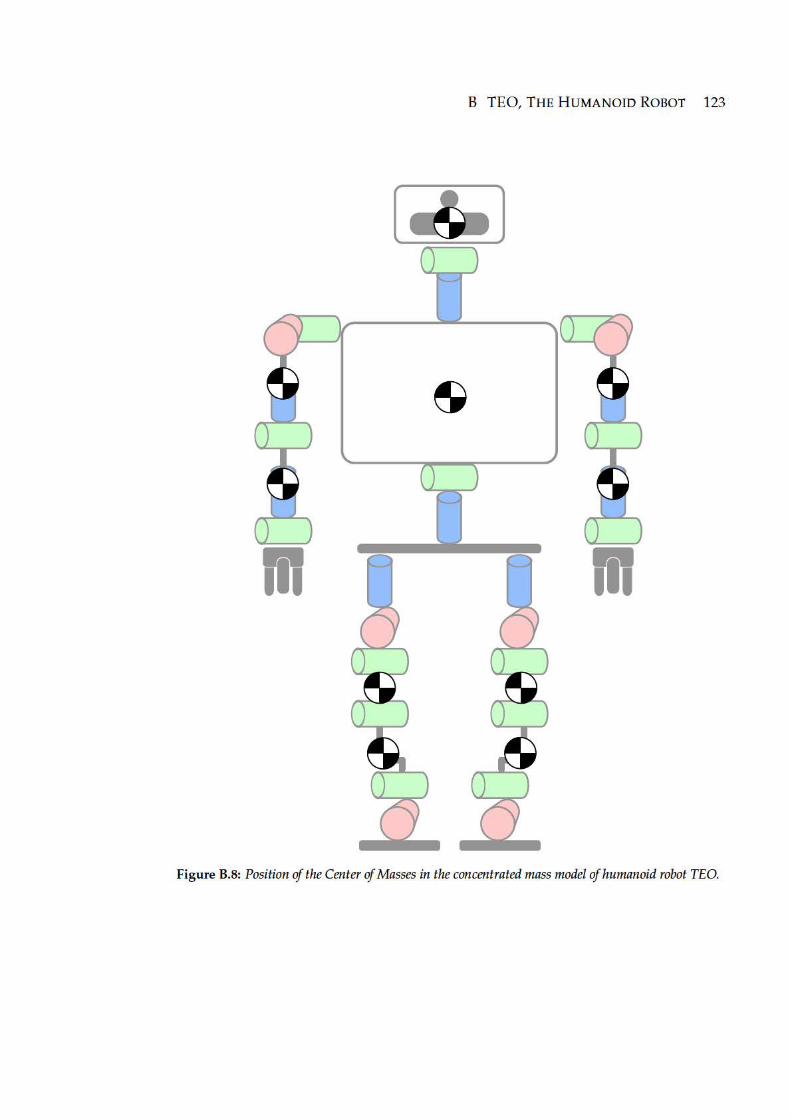

124 TEO, THE HUMANOID ROBOT
125
Bibliography
Akgun, B., Cakmak, M., Yoo, J. W., & Thomaz, A. L. (2012). Trajectories and keyframes
for kinesthetic teaching: A human-robot interaction perspective. In Proceedings
of the seventh annual acm/ieee international conference on human-robot interaction (pp.
391–398). (cited on p. 20.)
Albrecht, T. (2009). Dynamic time warping. In Information retrieval for music and motion
(pp. 69–84). Springer. (cited on pp. 38 and 51)
Ali Paikan, G. M., Paul Fitzpatrick, & Natale, L. (2014). Data flow ports monitoring
and arbitration. Journal of Software Engineering for Robotics, 5(1), 80-88. (cited on
p. 111.)
Alpaydin, E. (2014). Introduction to machine learning. MIT press. (cited on p. 37.)
An, C. H., Atkeson, C. G., & Hollerbach, J. M. (1988). Model-based control of a robot
manipulator (Vol. 214). MIT press Cambridge, MA. (cited on p. 22.)
Argall, B. D., Chernova, S., Veloso, M., & Browning, B. (2009). A survey of robot
learning from demonstration. Robotics and Autonomous Systems, 57(5), 469–483.
(cited on p. 19.)
Atkeson, C. G., & Schaal, S. (1997). Robot learning from demonstration. In Icml (Vol. 97,
pp. 12–20). (cited on p. 16.)
Bekkering, H., Wohlschlager, A., & Gattis, M. (2000). Imitation of gestures in children
is goal-directed. The Quarterly Journal of Experimental Psychology: Section A, 53(1),
153–164. (cited on pp. 12 and 14)
Billard, A., Epars, Y., Calinon, S., Schaal, S., & Cheng, G. (2004). Discovering optimal
imitation strategies. Robotics and Autonomous Systems, 47(2), 69–77. (cited on pp.
9 and 14)
126 BIBLIOGRAPHY
Billard, A. G., Calinon, S., & Guenter, F. (2006). Discriminative and adaptive imitation
in uni-manual and bi-manual tasks. Robotics and Autonomous Systems, 54(5), 370–
384. (cited on p. 20.)
Bona, B., & Indri, M. (2005). Friction compensation in robotics: an overview. In Ieee con-
ference on decision and control, 2005 and 2005 european control conference. cdc-ecc’05.
44th (pp. 4360–4367). (cited on p. 21.)
Bonaci, T., Herron, J., Yusuf, T., Yan, J., Kohno, T., & Chizeck, H. J. (2015). To make a
robot secure: An experimental analysis of cyber security threats against teleoper-
ated surgical robots.
(cited on p. 109.)
Calinon, S. (2009). Robot programming by demonstration: A probabilistic approach. EPFL
Press. (cited on p. 33.)
Calinon, S., & Billard, A. (2004). Stochastic gesture production and recognition model
for a humanoid robot. In Proceedings of ieee/rsj international conference on intelligent
robots and systems (iros 2004) (Vol. 3, pp. 2769–2774). (cited on p. 10.)
Calinon, S., & Billard, A. (2005). Recognition and reproduction of gestures using a
probabilistic framework combining pca, ica and hmm. In Proceedings of the 22nd
international conference on machine learning (pp. 105–112). (cited on p. 10.)
Calinon, S., & Billard, A. (2007). Incremental learning of gestures by imitation in a
humanoid robot. In Proceedings of the acm/ieee international conference on human-
robot interaction (pp. 255–262). (cited on p. 10.)
Calinon, S., D’halluin, F., Sauser, E. L., Caldwell, D. G., & Billard, A. G. (2010). Learning
and reproduction of gestures by imitation. IEEE Robotics & Automation Magazine,
17(2), 44–54. (cited on pp. 9, 20, and 48)
Calinon, S., Guenter, F., & Billard, A. (2005a). Goal-directed imitation in a humanoid
robot. In Proceedings of ieee international conference on robotics and automation, 2005
(icra 2005) (pp. 299–304). (cited on p. 14.)
Calinon, S., Guenter, F., & Billard, A. (2005b). Goal-directed imitation in a humanoid
robot. In Proceedings of the 2005 ieee international conference on robotics and automa-
tion. icra 2005 (pp. 299–304). (cited on p. 17.)
Calinon, S., Guenter, F., & Billard, A. (2007). On learning, representing, and generaliz-
ing a task in a humanoid robot. IEEE Transactions on Systems, Man, and Cybernetics,
Part B: Cybernetics, 37(2), 286–298. (cited on pp. 10 and 81)
BIBLIOGRAPHY 127
Canudas, C., Astrom, K., & Braun, K. (1987). Adaptive friction compensation in dc-
motor drives. IEEE Journal of Robotics and Automation, 3(6), 681–685. (cited on p.
21.)
Chernova, S., & Veloso, M. (2008). Multi-thresholded approach to demonstration se-
lection for interactive robot learning. In 3rd acm/ieee international conference on
human-robot interaction (hri) (pp. 225–232). (cited on p. 17.)
Chivers, D. S. (2012). Human action recognition by principal component analysis of motion
curves (Unpublished doctoral dissertation). Wright State University. (cited on p.
11.)
Coble, K., Wang, W., Chu, B., & Li, Z. (2010). Secure software attestation for military
telesurgical robot systems. In Military communications conference, 2010-milcom (pp.
965–970). (cited on p. 112.)
Denning, T., Matuszek, C., Koscher, K., Smith, J. R., & Kohno, T. (2009). A spotlight on
security and privacy risks with future household robots: attacks and lessons. In
Proceedings of the 11th international conference on ubiquitous computing (pp. 105–114).
(cited on p. 109.)
Dzung, D., Naedele, M., Von Hoff, T. P., & Crevatin, M. (2005). Security for industrial
communication systems. Proceedings of the IEEE, 93(6), 1152–1177. (cited on p.
112.)
Erlhagen, W., Mukovskiy, A., Bicho, E., Panin, G., Kiss, C., Knoll, A., . . . Bekkering,
H. (2006). Goal-directed imitation for robots: A bio-inspired approach to action
understanding and skill learning. Robotics and autonomous systems, 54(5), 353–360.
(cited on p. 14.)
Friedman, J., Hastie, T., & Tibshirani, R. (2001). The elements of statistical learning (Vol. 1).
Springer series in statistics Springer, Berlin. (cited on p. 38.)
Gallese, V., Fadiga, L., Fogassi, L., & Rizzolatti, G. (1996). Action recognition in the
premotor cortex. Brain, 119(2), 593–609. (cited on p. 12.)
Gomes, S. C. P., & Santos da Rosa, V. (2003). A new approach to compensate fric-
tion in robotic actuators. In Proceedings ieee international conference on robotics and
automation, 2003. icra’03. (Vol. 1, pp. 622–627). (cited on p. 22.)
Groza, B., & Dragomir, T.-L. (2008). Using a cryptographic authentication protocol
for the secure control of a robot over tcp/ip. In Ieee international conference on
automation, quality and testing, robotics. aqtr (Vol. 1, pp. 184–189). (cited on p. 112.)
128 BIBLIOGRAPHY
Guizzo, E., & Ackerman, E. (2012). The rise of the robot worker. Spectrum, IEEE, 49(10),
34–41. (cited on p. 21.)
Gupta, V., Gupta, S., Chang, S., & Stebila, D. (2002). Performance analysis of elliptic
curve cryptography for ssl. In Proceedings of the 1st acm workshop on wireless security
(pp. 87–94). (cited on p. 113.)
Hans, M., Graf, B., & Schraft, R. (2002). Robotic home assistant care-o-bot: Past-present-
future. In Proceedings of 11th ieee international workshop on robot and human interac-
tive communication (pp. 380–385). (cited on p. 109.)
Ijspeert, A. J., Nakanishi, J., & Schaal, S. (2002). Movement imitation with nonlinear
dynamical systems in humanoid robots. In Ieee international conference on robotics
and automation (icra) (Vol. 2, pp. 1398–1403). (cited on p. 19.)
Javaid, A. Y., Sun, W., Devabhaktuni, V. K., & Alam, M. (2012). Cyber security threat
analysis and modeling of an unmanned aerial vehicle system. In Ieee conference on
technologies for homeland security (hst) (pp. 585–590). (cited on p. 108.)
Jetchev, N., & Toussaint, M. (2011). Task space retrieval using inverse feedback control.
In Proceedings of the 28th international conference on machine learning (icml-11) (pp.
449–456). (cited on pp. 16 and 18)
Johnson, M., & Demiris, Y. (2004). Abstraction in recognition to solve the correspon-
dence problem for robot imitation. In Proceedings of towards autonomous robotic
systems (pp. 63–70). Springer. (cited on p. 14.)
Kermani, M. R., Wong, M., Patel, R. V., Moallem, M., & Ostojic, M. (2004). Friction com-
pensation in low and high-reversal-velocity manipulators. In Proceedings on ieee
international conference on robotics and automation, 2004. icra’04. (Vol. 5, pp. 4320–
4325). (cited on p. 22.)
King, H. H., Tadano, K., Donlin, R., Friedman, D., Lum, M. J., Asch, V., . . . Hannaford,
B. (2009). Preliminary protocol for interoperable telesurgery. In International
conference on advanced robotics. icar 2009 (pp. 1–6). (cited on p. 109.)
Kober, J., Mohler, B., & Peters, J. (2008). Learning perceptual coupling for motor prim-
itives. In Ieee/rsj international conference on intelligent robots and systems (iros) (pp.
834–839). (cited on p. 19.)
Kober, J., Wilhelm, A., Oztop, E., & Peters, J. (2012). Reinforcement learning to adjust
parametrized motor primitives to new situations. Autonomous Robots, 33(4), 361–
379. (cited on p. 19.)
BIBLIOGRAPHY 129
Kostic, D., de Jager, B., Steinbuch, M., & Hensen, R. (2004). Modeling and identifi-
cation for high-performance robot control: an rrr-robotic arm case study. IEEE
Transactions on Control Systems Technology, 12(6), 904–919. (cited on p. 22.)
Lee, G. S., & Thuraisingham, B. (2012). Cyberphysical systems security applied to
telesurgical robotics. Computer Standards & Interfaces, 34(1), 225–229. (cited on p.
112.)
Liu, M., & Quach, N. H. (2001). Estimation and compensation of gravity and friction
forces for robot arms: Theory and experiments. Journal of Intelligent and Robotic
Systems, 31(4), 339–354. (cited on p. 22.)
Luca, A. D., & Panzieri, S. (1993). Learning gravity compensation in robots: Rigid
arms, elastic joints, flexible links. International journal of adaptive control and signal
processing, 7(5), 417–433. (cited on p. 67.)
Luo, R. C., Yi, C., & Perng, Y. W. (2011). Gravity compensation and compliance based
force control for auxiliarily easiness in manipulating robot arm. In 2011 8th asian
control conference (ascc) (pp. 1193–1198). (cited on p. 22.)
Mallon, N., van de Wouw, N., Putra, D., & Nijmeijer, H. (2006). Friction compensation
in a controlled one-link robot using a reduced-order observer. IEEE Transactions
on Control Systems Technology, 14(2), 374–383. (cited on p. 94.)
Martin, P. K., & General, I. (2012). Nasa cybersecurity: An examination of the agency’s
information security. US House of Representatives, Feb. (cited on p. 109.)
Martınez, S., Monje, C. A., Jardon, A., Pierro, P., Balaguer, C., & Munoz, D. (2012). TEO:
Full-size humanoid robot design powered by a fuel cell system. Cybernetics and
Systems, 43(3), 163–180. (cited on pp. 74 and 86)
McClean, J., Stull, C., Farrar, C., & Mascarenas, D. (2013). A preliminary cyber-physical
security assessment of the robot operating system (ros). In Spie defense, security,
and sensing (pp. 874110–874110). (cited on p. 110.)
Metta, G., Fitzpatrick, P., & Natale, L. (2006). Yarp: yet another robot platform. Interna-
tional Journal on Advanced Robotics Systems, 3(1), 43–48. (cited on pp. 80 and 110)
Mickle, P. (1961). A peep into the automated future. (cited on p. 1.)
Mohammad, Y., & Nishida, T. (2013). Tackling the correspondence problem. In Active
media technology (pp. 84–95). Springer. (cited on p. 15.)
Mohanarajah, G., Hunziker, D., D’Andrea, R., & Waibel, M. (2015). Rapyuta: A cloud
robotics platform. IEEE Transactions on Automation Science and Engineering, 12(2),
130 BIBLIOGRAPHY
481–493. (cited on pp. 108 and 112)
Morante, S. (2012). Interfaz y librerıa para vision artificial, navegacion y seguimiento en
robotica (Tech. Rep.). Leganes: Universidad Carlos III de Madrid. (cited on p. 80.)
Morante, S., Victores, J. G., & Balaguer, C. (2015a). Automatic Demonstration and
Feature Selection for Robot Learning. In Ieee international conference on humanoid
robot - humanoids. Seoul: IEEE. (cited on pp. 7 and 35)
Morante, S., Victores, J. G., & Balaguer, C. (2015b). Cryptobotics: Why Robots Need
Cyber Safety. Frontiers in Robotics and AI, 2(23), 1–6. doi: 10.3389/frobt.2015.00023
(cited on p. 7.)
Morante, S., Victores, J. G., Jardon, A., & Balaguer, C. (2014). Action effect generaliza-
tion, recognition and execution through continuous goal-directed actions. In Ieee
international conference on robotics and automation (icra) (pp. 1822–1827). (cited on
pp. 6 and 34)
Morante, S., Victores, J. G., Jardon, A., & Balaguer, C. (2014). Action Effect Generaliza-
tion, Recognition and Execution through Continuous Goal-Directed Actions. In
Ieee international conference on robotics and automation (icra). (cited on p. 11.)
Morante, S., Victores, J. G., Jardon, A., & Balaguer, C. (2014). On using guided motor
primitives to execute continuous goal-directed actions. In Ro-man: The 23rd ieee
international symposium on robot and human interactive communication (pp. 613–618).
(cited on pp. 7 and 37)
Morante, S., Victores, J. G., Jardon, A., & Balaguer, C. (2015). Humanoid robot imitation
through continuous goal-directed actions: an evolutionary approach. Advanced
Robotics, 29(5), 303–314. (cited on p. 7.)
Morante, S., Victores, J. G., Martinez, S., & Balaguer, C. (2014). Sensorless friction and
gravity compensation. In 14th ieee-ras international conference on humanoid robots
(humanoids) (pp. 265–265). (cited on p. 98.)
Morante, S., Victores, J. G., Martinez de la casa, S., & Balaguer, C. (2015). Force-
Sensorless Friction and Gravity Compensation for Robots. In Robot 2015: Second
iberian robotics conference. Lisbon: SPR/SEIDROB. (cited on p. 7.)
Muhlig, M., Gienger, M., Hellbach, S., Steil, J. J., & Goerick, C. (2009). Task-level
imitation learning using variance-based movement optimization. In Ieee inter-
national conference on robotics and automation. icra’09 (pp. 1177–1184). (cited on pp.
16 and 17)
BIBLIOGRAPHY 131
Muhlig, M., Gienger, M., Steil, J. J., & Goerick, C. (2009). Automatic selection of task
spaces for imitation learning. In Ieee/rsj international conference on intelligent robots
and systems. iros 2009. (pp. 4996–5002). (cited on pp. 16 and 17)
Mulling, K., Kober, J., Kroemer, O., & Peters, J. (2013). Learning to select and general-
ize striking movements in robot table tennis. The International Journal of Robotics
Research, 32(3), 263–279. (cited on p. 19.)
Na, J., Chen, Q., Ren, X., & Guo, Y. (2014, Jan). Adaptive prescribed performance mo-
tion control of servo mechanisms with friction compensation. IEEE Transactions
on Industrial Electronics, 61(1), 486-494. doi: 10.1109/TIE.2013.2240635 (cited on
p. 22.)
Nehaniv, C. L., & Dautenhahn, K. (1999). Of hummingbirds and helicopters: An al-
gebraic framework for interdisciplinary studies of imitation and its applications.
In Interdisciplinary approaches to robot learning (Vol. 24, p. 136). World Scientific.
(cited on pp. 10 and 12)
Newton, I., Bernoulli, D., MacLaurin, C., & Euler, L. (1833). Philosophiae naturalis prin-
cipia mathematica (Vol. 1). excudit G. Brookman; impensis TT et J. Tegg, Londini.
(cited on p. 34.)
Olsson, H., Astrom, K. J., Canudas de Wit, C., Gafvert, M., & Lischinsky, P. (1998).
Friction models and friction compensation. European journal of control, 4(3), 176–
195. (cited on p. 21.)
Papadopoulos, E. G., & Chasparis, G. C. (2004). Analysis and model-based control
of servomechanisms with friction. Journal of dynamic systems, measurement, and
control, 126(4), 911–915. (cited on p. 22.)
Peters, J., Kober, J., Mulling, K., Kramer, O., & Neumann, G. (2013). Towards robot
skill learning: From simple skills to table tennis. In Machine learning and knowledge
discovery in databases (pp. 627–631). Springer. (cited on p. 19.)
Peters, J., & Schaal, S. (2008). Reinforcement learning of motor skills with policy gradi-
ents. Neural networks, 21(4), 682–697. (cited on p. 19.)
Pfleeger, C. P., & Pfleeger, S. L. (2002). Security in computing. Prentice Hall Professional
Technical Reference. (cited on p. 107.)
Press, W. H. (2007). Numerical recipes 3rd edition: The art of scientific computing. Cam-
bridge university press. (cited on p. 49.)
Quigley, M., Conley, K., Gerkey, B., Faust, J., Foote, T., Leibs, J., . . . Ng, A. Y. (2009). Ros:
132 BIBLIOGRAPHY
an open-source robot operating system. In Icra workshop on open source software
(Vol. 3, p. 5). (cited on p. 110.)
Rizzolatti, G., Fadiga, L., Gallese, V., & Fogassi, L. (1996). Premotor cortex and the
recognition of motor actions. Cognitive brain research, 3(2), 131–141. (cited on p.
12.)
Rochat, M. J., Caruana, F., Jezzini, A., Escola, L., Intskirveli, I., Grammont, F., . . . Umilta,
M. A. (2010, August). Responses of mirror neurons in area F5 to hand and tool
grasping observation. Experimental brain research, 204(4), 605–16. doi: 10.1007/
s00221-010-2329-9 (cited on p. 12.)
Saegusa, R., Metta, G., Sandini, G., & Natale, L. (2013). Developmental action per-
ception for manipulative interaction. In Ieee international conference on robotics and
automation (icra) (p. 4967-4972). (cited on p. 14.)
Schaal, S. (1999). Is imitation learning the route to humanoid robots? Trends in cognitive
sciences, 3(6), 233–242. (cited on pp. 10 and 18)
Schaal, S. (2006). Dynamic movement primitives-a framework for motor control in
humans and humanoid robotics. In Adaptive motion of animals and machines (pp.
261–280). Springer. (cited on p. 33.)
Schaal, S., Ijspeert, A., & Billard, A. (2003). Computational approaches to motor learn-
ing by imitation. Philosophical Transactions of the Royal Society of London. Series B:
Biological Sciences, 358(1431), 537–547. (cited on p. 18.)
Sciavicco, L., & Villani, L. (2009). Robotics: modelling, planning and control. Springer.
(cited on p. 67.)
Subramanian, K., & Suresh, S. (2012). Human action recognition using meta-cognitive
neuro-fuzzy inference system. International journal of neural systems, 22(06). (cited
on p. 11.)
Tanenbaum, A. S. (2009). Modern Operating Systems (3rd ed.). Pearson-Prentice Hall.
(cited on p. 108.)
Tarsitano, I. A.-A. (2012). Adjusting time series of possible unequal lengths. In Sis.
proceedings of the xlvi scientific meeting (pp. 1–4). (cited on p. 16.)
Toris, R., Shue, C., & Chernova, S. (2014, April). Message authentication codes for
secure remote non-native client connections to ros enabled robots. In Ieee inter-
national conference on technologies for practical robot applications (tepra) (p. 1-6). doi:
10.1109/TePRA.2014.6869141 (cited on p. 111.)
BIBLIOGRAPHY 133
Traversaro, S., Del Prete, A., Muradore, R., Natale, L., & Nori, F. (2013). Inertial param-
eter identification including friction and motor dynamics. In Ieee-ras international
conference on humanoid robots (humanoid’13), atlanta, usa. (cited on p. 22.)
Ugur, E., Sahin, E., & Oztop, E. (2012). Self-discovery of motor primitives and learning
grasp affordances. In Ieee/rsj international conference on intelligent robots and systems
(iros) (pp. 3260–3267). (cited on p. 19.)
Victores, J. G., Morante, S., Jardon, A., & Balaguer, C. (2013a). Semantic action param-
eter inference through machine learning methods. In Robocity2030 12th workshop
robotica cognitiva. (cited on p. 13.)
Victores, J. G., Morante, S., Jardon, A., & Balaguer, C. (2013b). Towards Robot Imag-
ination Through Object Feature Inference. In Proceedings of ieee/rsj international
conference on intelligent robots and systems (iros 2013). IEEE. (cited on p. 104.)
Virgala, I., & Kelemen, M. (2013). Experimental friction identification of a dc motor.
International Journal of Mechanics and Applications, 3(1), 26–30. (cited on pp. 68
and 95)
Vuong, T., Filippoupolitis, A., Loukas, G., & Gan, D. (2014). Physical indicators of cyber
attacks against a rescue robot. In Ieee international conference on pervasive computing
and communications workshops (percom workshops) (pp. 338–343). (cited on p. 110.)
Yamashita, Y., & Tani, J. (2008). Emergence of functional hierarchy in a multiple
timescale neural network model: a humanoid robot experiment. PLoS Comput
Biol, 4(11), e1000220. (cited on p. 15.)
Recommended