Tutorial (Beginner level):Orthomosaic and DEM Generation with Agisoft PhotoScan Pro 1.2

(with Ground Control Points)

OverviewAgisoft PhotoScan Professional allows to generate georeferenced dense point clouds, textured polygonal models, digital elevation models and orthomosaics from a set of overlapping images with the corresponding referencing information. This tutorial describes the main processing steps of DEM/Orthomosaic generation workflow for a set of images with the ground control points.

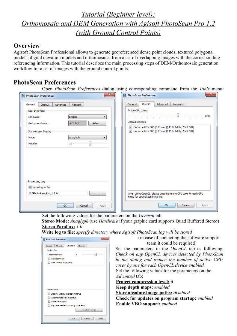
PhotoScan PreferencesOpen PhotoScan Preferences dialog using corresponding command from the Tools menu:

Set the following values for the parameters on the General tab:Stereo Mode: Anaglyph (use Hardware if your graphic card supports Quad Buffered Stereo)Stereo Parallax: 1.0Write log to file: specify directory where Agisoft PhotoScan log will be stored

(in case of contacting the software support team it could be required)

Set the parameters in the OpenCL tab as following: Check on any OpenCL devices detected by PhotoScan in the dialog and reduce the number of active CPU cores by one for each OpenCL device enabled.Set the following values for the parameters on the Advanced tab:Project compression level: 6Keep depth maps: enabledStore absolute image paths: disabledCheck for updates on program startup: enabledEnable VBO support: enabled

Add PhotosTo add photos select Add Photos... command from the Workflow menu or click Add Photos button

located on Workspace toolbar.In the Add Photos dialog browse the source folder and select files to be processed. Click Open button.

Load Camera Positions At this step coordinate system for the future model is set using camera positions.

Note: If camera positions are unknown this step could be skipped. The align photos procedure, however, will take more time in this case.

Open Reference pane using the corresponding command from the View menu. Click Import button on the Reference pane toolbar and select the file containing camera positions

information in the Open dialog. The easiest way is to load simple character-separated file (*.txt) that contains x- and y- coordinates

and height for each camera position (camera orientation data, i.e. pitch, roll and yaw values, could also be imported, but the data is not obligatory to reference the model).

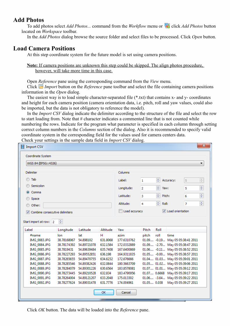
In the Import CSV dialog indicate the delimiter according to the structure of the file and select the row to start loading from. Note that # character indicates a commented line that is not counted while numbering the rows. Indicate for the program what parameter is specified in each column through setting correct column numbers in the Columns section of the dialog. Also it is recommended to specify valid coordinate system in the corresponding field for the values used for camera centers data.Check your settings in the sample data field in Import CSV dialog.

Click OK button. The data will be loaded into the Reference pane.

Import EXIF button located on the Reference pane can also be used to load camera positions information if EXIF meta-data is available.

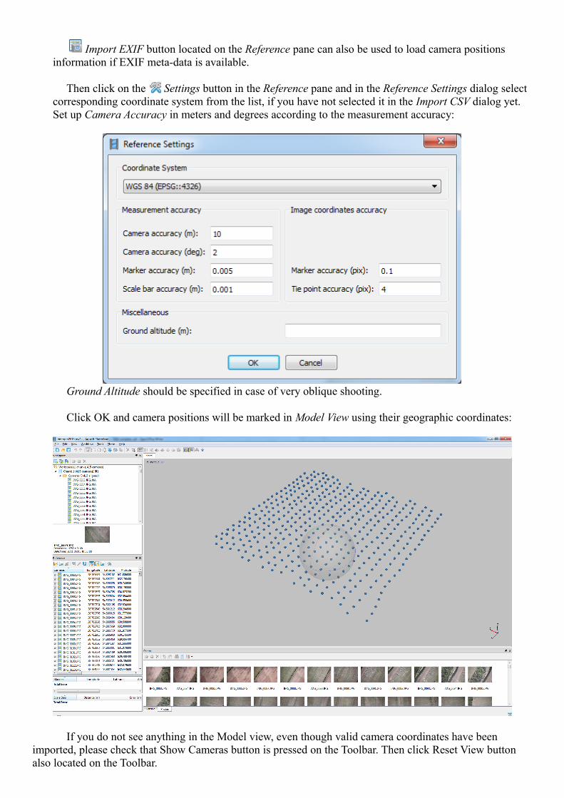
Then click on the Settings button in the Reference pane and in the Reference Settings dialog select corresponding coordinate system from the list, if you have not selected it in the Import CSV dialog yet. Set up Camera Accuracy in meters and degrees according to the measurement accuracy:

Ground Altitude should be specified in case of very oblique shooting.

Click OK and camera positions will be marked in Model View using their geographic coordinates:

If you do not see anything in the Model view, even though valid camera coordinates have been imported, please check that Show Cameras button is pressed on the Toolbar. Then click Reset View button also located on the Toolbar.

Check Camera Calibration

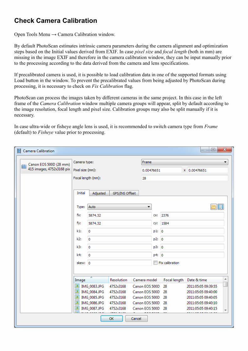
Open Tools Menu → Camera Calibration window.

By default PhotoScan estimates intrinsic camera parameters during the camera alignment and optimization steps based on the Initial values derived from EXIF. In case pixel size and focal length (both in mm) are missing in the image EXIF and therefore in the camera calibration window, they can be input manually prior to the processing according to the data derived from the camera and lens specifications.

If precalibrated camera is used, it is possible to load calibration data in one of the supported formats using Load button in the window. To prevent the precalibrated values from being adjusted by PhotoScan during processing, it is necessary to check on Fix Calibration flag.

PhotoScan can process the images taken by different cameras in the same project. In this case in the left frame of the Camera Calibration window multiple camera groups will appear, split by default according to the image resolution, focal length and pixel size. Calibration groups may also be split manually if it is necessary.

In case ultra-wide or fisheye angle lens is used, it is recommended to switch camera type from Frame (default) to Fisheye value prior to processing.

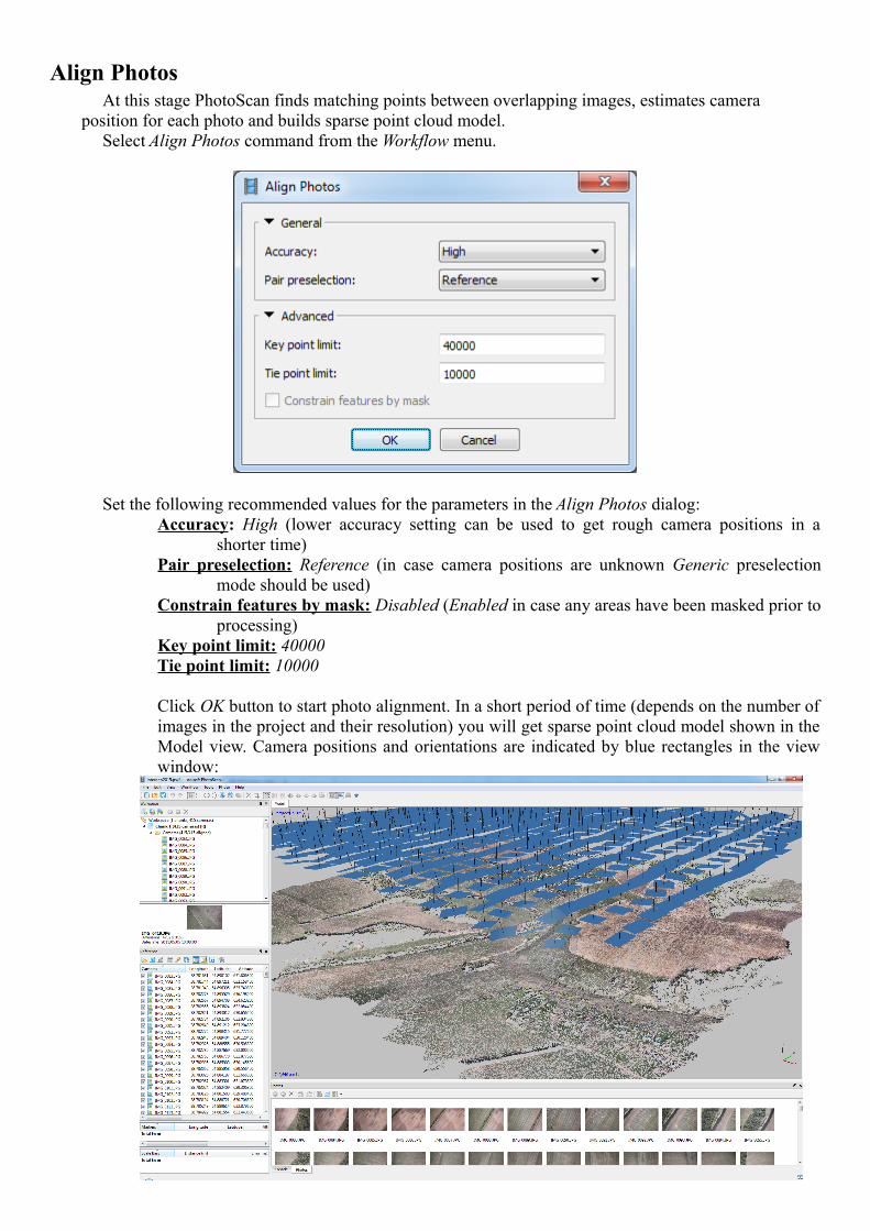
Align PhotosAt this stage PhotoScan finds matching points between overlapping images, estimates camera

position for each photo and builds sparse point cloud model.Select Align Photos command from the Workflow menu.

Set the following recommended values for the parameters in the Align Photos dialog:Accuracy: High (lower accuracy setting can be used to get rough camera positions in a

shorter time)Pair preselection: Reference (in case camera positions are unknown Generic preselection

mode should be used)Constrain features by mask: Disabled (Enabled in case any areas have been masked prior to

processing)Key point limit: 40000 Tie point limit: 10000

Click OK button to start photo alignment. In a short period of time (depends on the number of images in the project and their resolution) you will get sparse point cloud model shown in the Model view. Camera positions and orientations are indicated by blue rectangles in the view window:

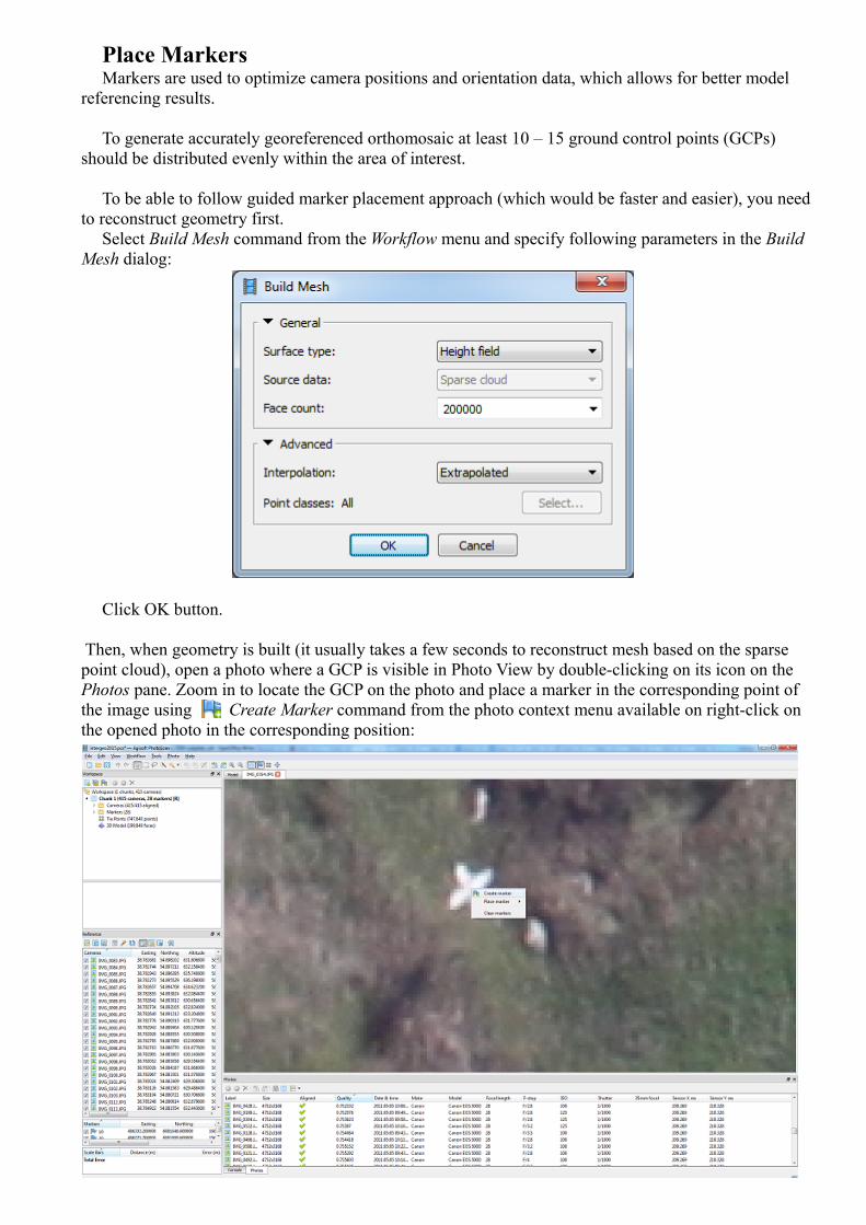
Place Markers Markers are used to optimize camera positions and orientation data, which allows for better model

referencing results.

To generate accurately georeferenced orthomosaic at least 10 – 15 ground control points (GCPs) should be distributed evenly within the area of interest.

To be able to follow guided marker placement approach (which would be faster and easier), you need to reconstruct geometry first.

Select Build Mesh command from the Workflow menu and specify following parameters in the Build Mesh dialog:

Click OK button.

Then, when geometry is built (it usually takes a few seconds to reconstruct mesh based on the sparse point cloud), open a photo where a GCP is visible in Photo View by double-clicking on its icon on the Photos pane. Zoom in to locate the GCP on the photo and place a marker in the corresponding point of the image using Create Marker command from the photo context menu available on right-click on the opened photo in the corresponding position:

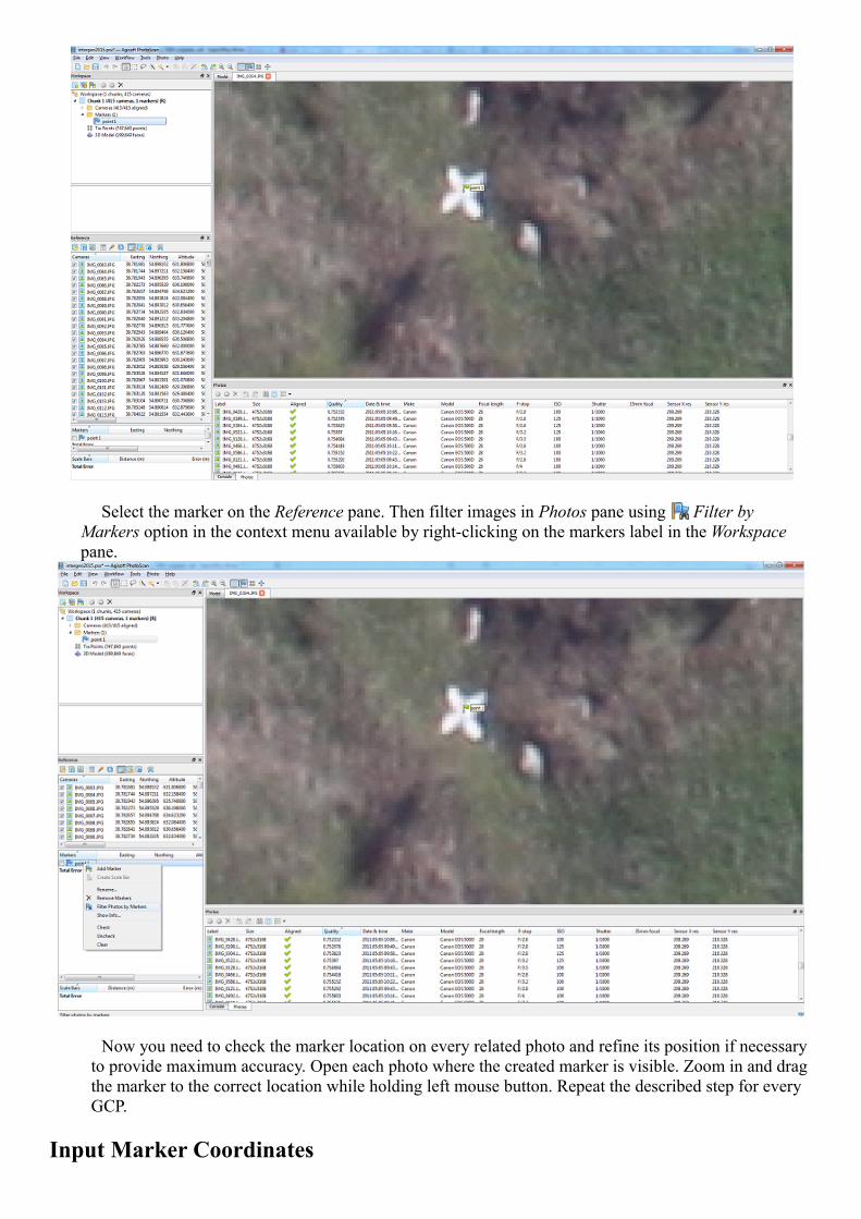
Select the marker on the Reference pane. Then filter images in Photos pane using Filter by Markers option in the context menu available by right-clicking on the markers label in the Workspace pane.

Now you need to check the marker location on every related photo and refine its position if necessary

to provide maximum accuracy. Open each photo where the created marker is visible. Zoom in and drag the marker to the correct location while holding left mouse button. Repeat the described step for every GCP.

Input Marker Coordinates

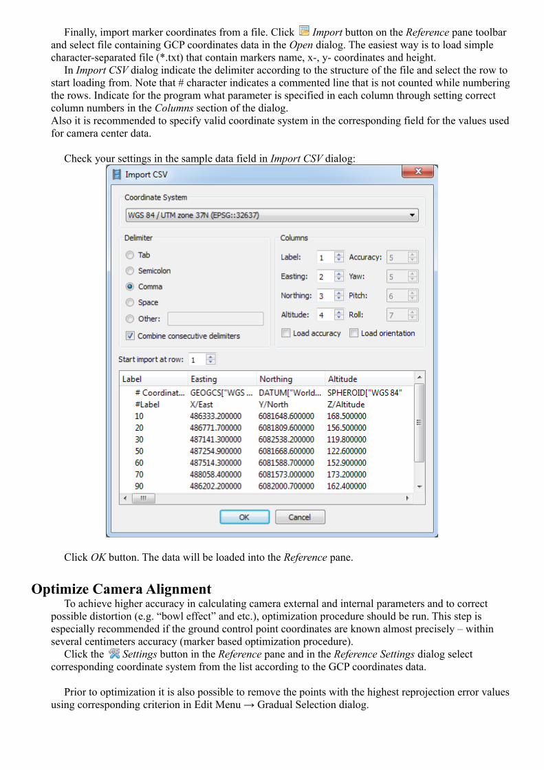
Finally, import marker coordinates from a file. Click Import button on the Reference pane toolbar and select file containing GCP coordinates data in the Open dialog. The easiest way is to load simple character-separated file (*.txt) that contain markers name, x-, y- coordinates and height.

In Import CSV dialog indicate the delimiter according to the structure of the file and select the row to start loading from. Note that # character indicates a commented line that is not counted while numbering the rows. Indicate for the program what parameter is specified in each column through setting correct column numbers in the Columns section of the dialog.Also it is recommended to specify valid coordinate system in the corresponding field for the values used for camera center data.

Check your settings in the sample data field in Import CSV dialog:

Click OK button. The data will be loaded into the Reference pane.

Optimize Camera Alignment To achieve higher accuracy in calculating camera external and internal parameters and to correct

possible distortion (e.g. “bowl effect” and etc.), optimization procedure should be run. This step is especially recommended if the ground control point coordinates are known almost precisely – within several centimeters accuracy (marker based optimization procedure).

Click the Settings button in the Reference pane and in the Reference Settings dialog select corresponding coordinate system from the list according to the GCP coordinates data.

Prior to optimization it is also possible to remove the points with the highest reprojection error values using corresponding criterion in Edit Menu → Gradual Selection dialog.

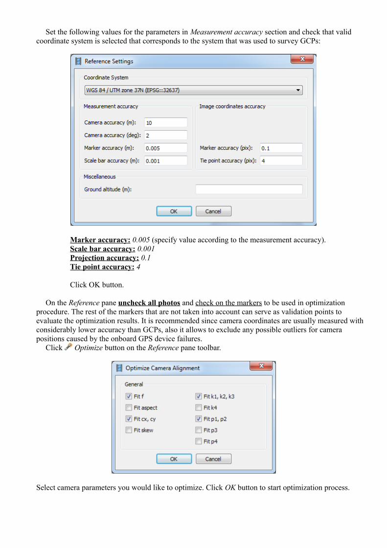
Set the following values for the parameters in Measurement accuracy section and check that valid coordinate system is selected that corresponds to the system that was used to survey GCPs:

Marker accuracy: 0.005 (specify value according to the measurement accuracy).Scale bar accuracy: 0.001 Projection accuracy: 0.1Tie point accuracy: 4

Click OK button.

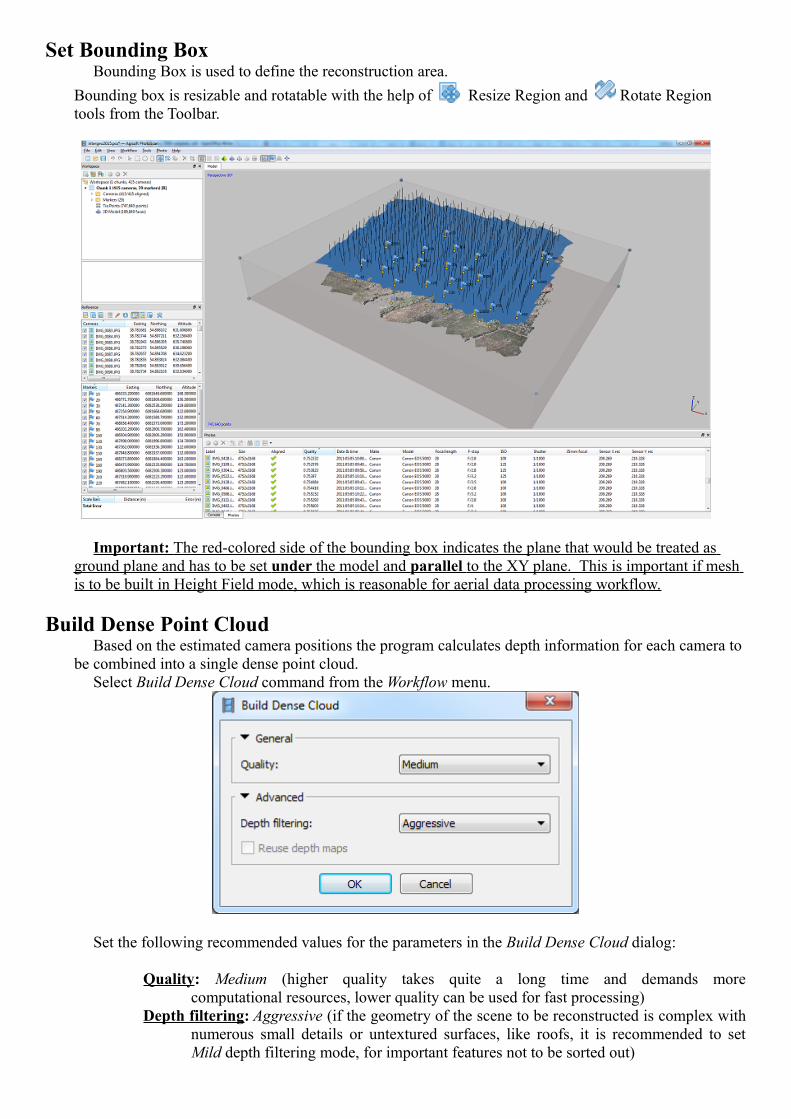
On the Reference pane uncheck all photos and check on the markers to be used in optimization procedure. The rest of the markers that are not taken into account can serve as validation points to evaluate the optimization results. It is recommended since camera coordinates are usually measured with considerably lower accuracy than GCPs, also it allows to exclude any possible outliers for camera positions caused by the onboard GPS device failures.

Click Optimize button on the Reference pane toolbar.

Select camera parameters you would like to optimize. Click OK button to start optimization process.

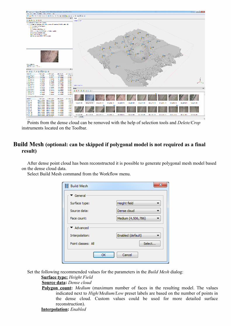
Set Bounding Box Bounding Box is used to define the reconstruction area.

Bounding box is resizable and rotatable with the help of Resize Region and Rotate Region tools from the Toolbar.

Important: The red-colored side of the bounding box indicates the plane that would be treated as ground plane and has to be set under the model and parallel to the XY plane. This is important if mesh is to be built in Height Field mode, which is reasonable for aerial data processing workflow.

Build Dense Point Cloud Based on the estimated camera positions the program calculates depth information for each camera to

be combined into a single dense point cloud.Select Build Dense Cloud command from the Workflow menu.

Set the following recommended values for the parameters in the Build Dense Cloud dialog:

Quality: Medium (higher quality takes quite a long time and demands more computational resources, lower quality can be used for fast processing)

Depth filtering: Aggressive (if the geometry of the scene to be reconstructed is complex with numerous small details or untextured surfaces, like roofs, it is recommended to set Mild depth filtering mode, for important features not to be sorted out)

Points from the dense cloud can be removed with the help of selection tools and Delete/Crop instruments located on the Toolbar.

Build Mesh (optional: can be skipped if polygonal model is not required as a final result)

After dense point cloud has been reconstructed it is possible to generate polygonal mesh model based on the dense cloud data.

Select Build Mesh command from the Workflow menu.

Set the following recommended values for the parameters in the Build Mesh dialog:Surface type: Height FieldSource data: Dense cloud Polygon count: Medium (maximum number of faces in the resulting model. The values

indicated next to High/Medium/Low preset labels are based on the number of points in the dense cloud. Custom values could be used for more detailed surface reconstruction).

Interpolation: Enabled

Click OK button to start mesh reconstruction.

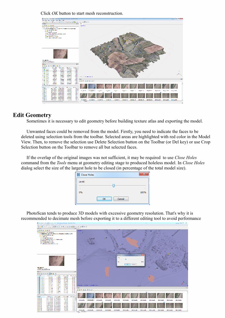
Edit GeometrySometimes it is necessary to edit geometry before building texture atlas and exporting the model.

Unwanted faces could be removed from the model. Firstly, you need to indicate the faces to be deleted using selection tools from the toolbar. Selected areas are highlighted with red color in the Model View. Then, to remove the selection use Delete Selection button on the Toolbar (or Del key) or use Crop Selection button on the Toolbar to remove all but selected faces.

If the overlap of the original images was not sufficient, it may be required to use Close Holes command from the Tools menu at geometry editing stage to produced holeless model. In Close Holes dialog select the size of the largest hole to be closed (in percentage of the total model size).

PhotoScan tends to produce 3D models with excessive geometry resolution. That's why it is recommended to decimate mesh before exporting it to a different editing tool to avoid performance

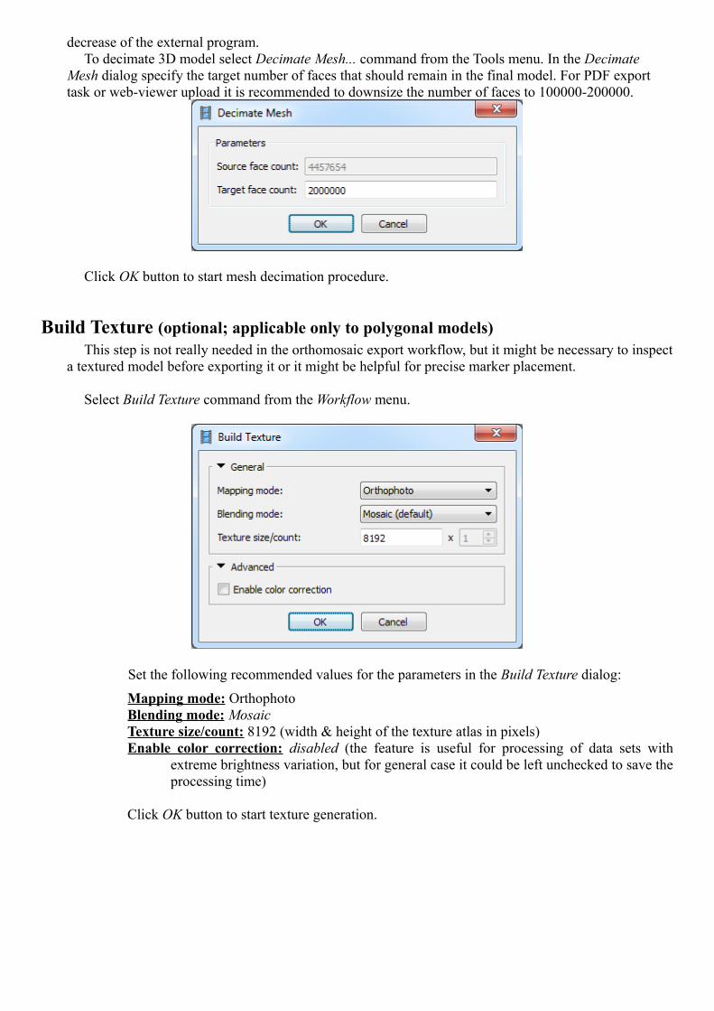
decrease of the external program. To decimate 3D model select Decimate Mesh... command from the Tools menu. In the Decimate

Mesh dialog specify the target number of faces that should remain in the final model. For PDF export task or web-viewer upload it is recommended to downsize the number of faces to 100000-200000.

Click OK button to start mesh decimation procedure.

Build Texture (optional; applicable only to polygonal models)This step is not really needed in the orthomosaic export workflow, but it might be necessary to inspect

a textured model before exporting it or it might be helpful for precise marker placement.

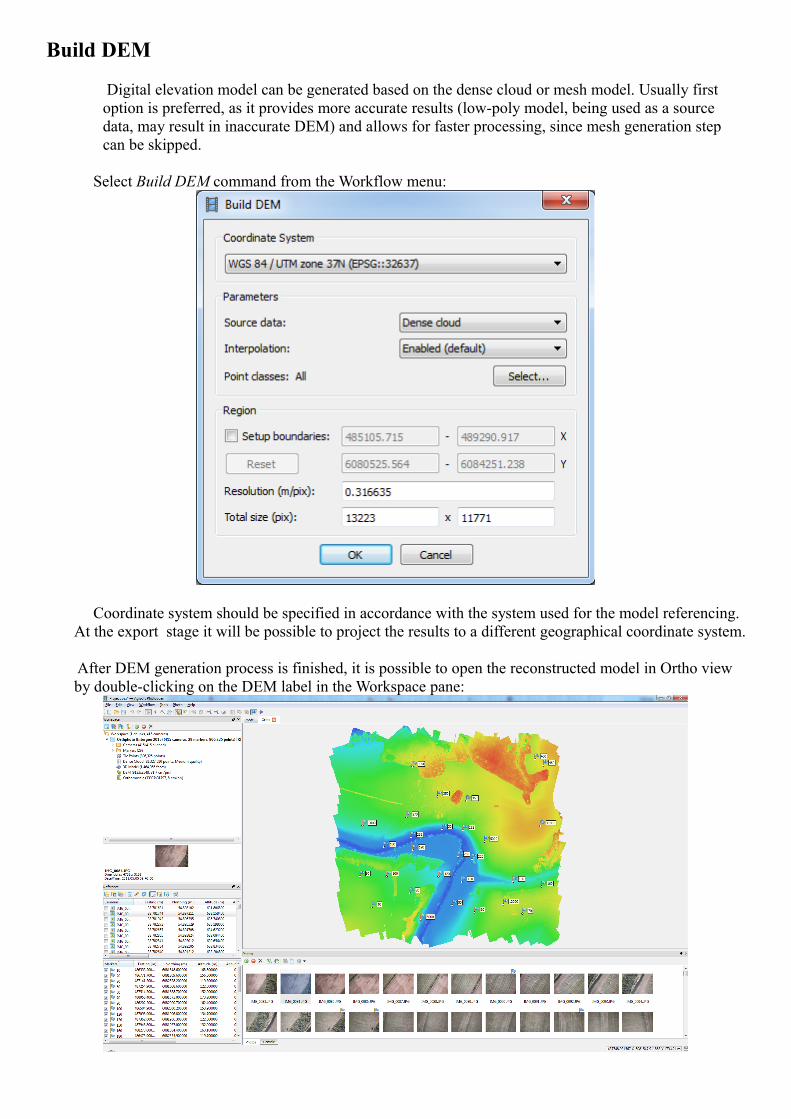
Select Build Texture command from the Workflow menu.

Set the following recommended values for the parameters in the Build Texture dialog:

Mapping mode: OrthophotoBlending mode: MosaicTexture size/count: 8192 (width & height of the texture atlas in pixels)Enable color correction: disabled (the feature is useful for processing of data sets with

extreme brightness variation, but for general case it could be left unchecked to save the processing time)

Click OK button to start texture generation.

Build DEM

Digital elevation model can be generated based on the dense cloud or mesh model. Usually first option is preferred, as it provides more accurate results (low-poly model, being used as a source data, may result in inaccurate DEM) and allows for faster processing, since mesh generation step can be skipped.

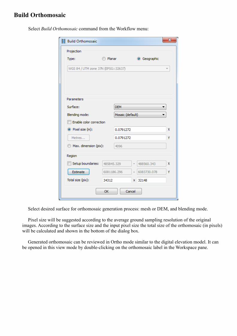
Select Build DEM command from the Workflow menu:

Coordinate system should be specified in accordance with the system used for the model referencing. At the export stage it will be possible to project the results to a different geographical coordinate system.

After DEM generation process is finished, it is possible to open the reconstructed model in Ortho view by double-clicking on the DEM label in the Workspace pane:

Build Orthomosaic

Select Build Orthomosaic command from the Workflow menu:

Select desired surface for orthomosaic generation process: mesh or DEM, and blending mode.

Pixel size will be suggested according to the average ground sampling resolution of the original images. According to the surface size and the input pixel size the total size of the orthomosaic (in pixels) will be calculated and shown in the bottom of the dialog box.

Generated orthomosaic can be reviewed in Ortho mode similar to the digital elevation model. It can be opened in this view mode by double-clicking on the orthomosaic label in the Workspace pane.

Export Orthomosaic

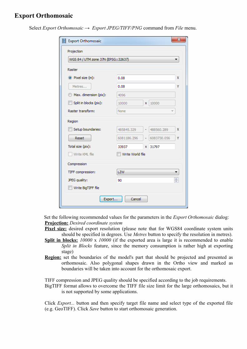
Select Export Orthomosaic → Export JPEG/TIFF/PNG command from File menu.

Set the following recommended values for the parameters in the Export Orthomosaic dialog:Projection: Desired coordinate systemPixel size: desired export resolution (please note that for WGS84 coordinate system units

should be specified in degrees. Use Metres button to specify the resolution in metres).Split in blocks: 10000 x 10000 (if the exported area is large it is recommended to enable

Split in Blocks feature, since the memory consumption is rather high at exporting stage)

Region: set the boundaries of the model's part that should be projected and presented as orthomosaic. Also polygonal shapes drawn in the Ortho view and marked as boundaries will be taken into account for the orthomosaic export.

TIFF compression and JPEG quality should be specified according to the job requirements.BigTIFF format allows to overcome the TIFF file size limit for the large orthomosaics, but it

is not supported by some applications.

Click Export... button and then specify target file name and select type of the exported file (e.g. GeoTIFF). Click Save button to start orthomosaic generation.

Export DEM

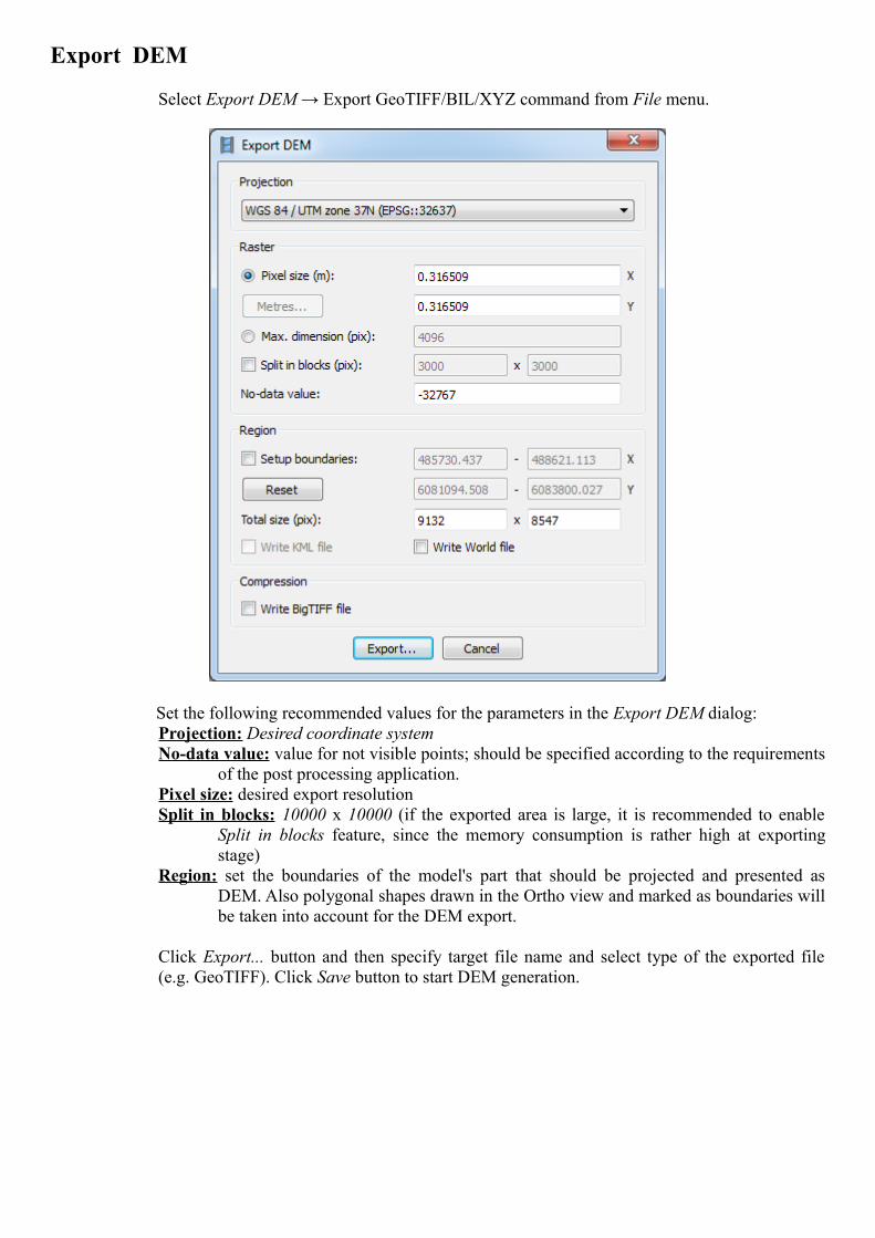
Select Export DEM → Export GeoTIFF/BIL/XYZ command from File menu.

Set the following recommended values for the parameters in the Export DEM dialog:Projection: Desired coordinate systemNo-data value: value for not visible points; should be specified according to the requirements

of the post processing application.Pixel size: desired export resolution Split in blocks: 10000 x 10000 (if the exported area is large, it is recommended to enable

Split in blocks feature, since the memory consumption is rather high at exporting stage)

Region: set the boundaries of the model's part that should be projected and presented as DEM. Also polygonal shapes drawn in the Ortho view and marked as boundaries will be taken into account for the DEM export.

Click Export... button and then specify target file name and select type of the exported file (e.g. GeoTIFF). Click Save button to start DEM generation.