A Comparison of Orthomosaic Software for Use with Ultra High

Resolution Imagery of a Wetland Environment

John W. Gross a

a Center for Geographic Information Science and Geography Department, Central Michigan University, Mt. Pleasant, MI 48859

Abstract

Unmanned aerial systems are becoming popular in numerous military, civil, and research

applications as a platform for the collection of ultra-high spatial resolution imagery in a cost-

effective, dynamic manner. The use of unmanned aerial systems, however, requires significant

CPU intensive pre-processing to convert hundreds of raw images into a single usable

representation of the earth’s surface. The goal of this study is to compare geometric accuracy,

visual quality, ease of use and cost of Photoscan Pro, Pix4D Pro Mapper and Microsoft Image

Composite Editor; three modern image stitching software packages which have the potential to

significantly decrease the amount of time and user input required for creating orthomosaics. 223

usable images with spatial resolutions of 1.26 cm were collected on 26 September 2014 using an

unmanned aerial system. Photoscan Pro, Pix4d Pro Mapper, and Image Composite Editor were

used to create orthomosaics from the individual images. All orthomosaics were georeferenced

using 54 ground control points collected during the field season. The geometric accuracy of the

orthomosaics was calculated using the root mean square error of 17 validation points. Statistical

analysis was used to examine the level of significance between the different software’s. Microsoft

Image Composite Editor had significantly fewer visual errors (Chi Square, p < .001) but, it had the

poorest geometric accuracy with an RMSE of 34.7 cm (Tukey-Kramer, p < 0.05). Photoscan

Professional had the most visual errors (Chi Square, p < 0.001), and an RMSE of 10.9 cm. Pix4D

Pro had the best geometric accuracy with an RMSE of 7.7 cm, however this was not found to be

statistically different from Photoscan (Tukey-Kramer, p > 0.05). These results suggest that there

is no single best choice in terms of image stitching software, and that software selection must be

made on the budget and geometric and visual quality requirements of the individual project.

1. Introduction

Unmanned aerial systems (UASs), have been used, in varying forms since the 1930’s,

primarily in military applications (http://www.science.smith.edu/cmet/safetycode/faq.html;

Degarmo, 2004). Since the early 2000’s, however, the possible capabilities of UAVs in civil

applications such as biological research, precision agriculture, and archeology have become well

documented (Knoth et al, 2013; Verhoeven 2011; Verhoeven 2012; Zhenkun et al, 2013). This

growth will likely continue as government regulations and safety practices adapt to meet

demands (Zweig et al., 2014). The primary use of UAS in civil applications is as a platform for

the collection of ultra-high resolution (sub-decimeter) imagery. The use of such miniaturized

platforms and consumer-grade sensor equipment, however, leads to the collection of hundreds of

individual images which typically lack, or it exists but is of questionable accuracy, much of the

ancillary information commonly used in traditional airphoto interpretation. This lack of accurate

information translates into the requirement for novel techniques to convert these hundreds of

images into a single usable representation of the earth’s surface.

Many UAS studies have utilized consumer grade available digital cameras (Laliberte et

al, 2008).The use of such cameras combined with the small UAS platform can potentially create

a number of problems. There can be significant variability in rotational and angular camera

position, degree of overlap, and illumination (Barazzetti et al, 2010). The low flight altitude of

the UAS in relation to changes in ground elevation can lead to significant perspective distortions

(Zhang et al, 2011). Also, the global positions systems (GPS) and inertial measurement units on

board the UAS are typically too inaccurate to be meaningful, leading to significant errors in the

external operating parameters (EO) of the imagery (Laliberte et al, 2007; Turner et al, 2012).

Such errors, combined with the large number of images, make conventional photogrammetric

techniques difficult, if not impossible.

Recent advancements in the fields of photogrammetry and computer vision have

produced a number of algorithms that have the potential to not only handle these issues, but to do

so in a highly automated fashion. Such algorithms are able to detect and match hundreds of

overlapping images, accurately estimate internal and external camera parameters, create point

cloud representations of the 3D surface, and combine everything into a single, seamless 3D

model or orthomosaic. One of the most notable sets of algorithms for this purpose is structure

from motion (SfM). SfM is of benefit because it does not require a priori knowledge of any

camera parameters or scene information (Choudhary, 2012; Westoby et al, 2012). SfM typically

utilizes scale invariant feature transform (SIFT) to locate important features known as keypoints.

SIFT locates keypoints in an image using a difference-of-Gaussian function (Lowe, 2004).

Keypoints are then matched in each image based on the minimization of Euclidian distance

(Lindeberg, 2012). These keypoints are then tracked from image to image enabling the accurate

estimation of both camera orientation as well as keypoint location (Westoby et al, 2012). These

keypoints become a dense cloud allowing for the construction of a 3D representation of the

scene.

Previous research has utilized a variety of homemade SfM scripts to varying degrees of

success. Laliberte et al. (2008) flew imagery over the Jornada Experimental Range in southern

New Mexico. They used Autopano pro, a SIFT based software, to generate keypoints. These

keypoints were included in a custom script known as PreSync which also incorporated a 1 m

digital orthoquad and a 10 m digital elevation model to adjust and improve existing EOs. The

original images as well as the updated EOs were then put into Leica Photogrammetric Suite to

generate the mosaic. They were able to obtain overall RMSE of 47.9 cm which in part was due to

a lack of differential correction on their GPS unit. Turner et al 2012 created an automated

technique using SIFT and SfM techniques to automate the mosaicking of imagery collected over

two sites of an Antarctic moss bed. They were able to achieve mean absolute total errors ranging

from .103 m to 1.247 m.

Since 2010 a number of commercial SfM software packages have become available. Two

of the most popular include Photoscan Professional (Photoscan), and Pix4D Mapper Pro

(Pix4D). Both these software have been successfully used in current research (Vallet et al. 2011;

Kung et a.l 2011a; Kung et al. 2011b; Verhoeven et al.2011; Verhoeven et al. 2012; Woodget et

al. 2014).

The goal of this research was to compare software packages for use with imagery

acquired by UAS. Two commercially available Sfm software packages Photoscan and Pix4D

were compared as well as Microsoft Image Composite Editor (ICE) a freeware available through

Microsoft, which does not create a 3D point cloud, but rather stiches the images together

directly. This analysis focused on four main components: ease of use, visual quality, geometric

accuracy, and cost. Previous comparisons have reported that Photoscan Pro was the more

accurate software based primarily on digital surface modeling results and not a quantitative

analysis of image quality. (Sona et al. 2014; Turner et al. 2014),

2. Data

969 images were collected on 26 September 2014 at Braeburn Marsh Preserve near Ann

Arbor Michigan, USA (~42° 16’ N, ~84° 4’W). Imagery was collected using a Cannon EOS 6D

digital single lens reflex camera with a 50mm fixed focal length lens at a flight of 100m.The

camera was mounted on a Leptron Avenger airframe (Leptron, Golden, CO). All mission

parameters and flight limits were monitored and controlled via a ground station using piccolo

command center (Cloud Cap Technology, Hood River, OR). After the removal of low quality

images and turns in the flight lines (which reduce the accuracy of the final product), only 224

images were retained for analysis, covering 15.5 acres with a spatial resolution of 1.26 cm. Due

to the low accuracy of the camera GPS (25 m) no GPS EXIF data was retained for the analysis.

Ground control points (GCP) were established prior in the field season using a R8 GNSS

RTK rover and a TCS3 hand held unit (Trimble Navigation Limited, Sunnyvale, California) with

a recorded horizontal accuracy of +- 2 cm (95% confidence interval). Each point was marked

with a metal pole and colored foam for easy recognition in the imagery. A total of 70 points were

collected.

3. Methods

3.1 Overview

The 224 images, and 53 GCPs were used to create an image mosaic. The image mosaic

was created using all three software packages; Photoscan Pro, Pix4D, and ICE. The resultant

mosaics were then subjected to geometric and visual quality assessments and statistical analysis.

A basic workflow of the methodology can be seen in figure 1.

Figure 1: Basic workflow of methodology

3.2 Photoscan Pro

Created by the Russian based company Agisoft in 2010, Photoscan Pro is a 3D model and

image stitching software package. It utilizes an adapted form of the popular structure from

motion technology known as the scale invariant feature transformation proposed by Lowe

(2004). At its core this process uses feature points, which are simply geometrically similar and

distinct regions in an image e.g. building corners or the top of light posts. These points are then

tracked across multiple images creating a series of connections between photographs

(Verhoeven, 2011). In addition, this algorithm allows Photoscan Pro to automatically and

accurately estimate a large number of internal and external camera parameters which previously

had to be known and entered manually. Utilizing such algorithms, software packages such as

Photoscan Pro are capable of matching images at the subpixel level (Woodget et al., 2014).

The Photoscan Pro workflow can be broken down into four basic steps: image alignment,

dense point cloud formation, mesh creation, and texture creation. Each of these steps are run

independent of each other, and aside from the inclusion of ground control points they can be run

with little to no user input. It is also important to note that these stages are all independent and

can be saved separately for later use or revision.

There are a number of parameters that must be defined, often with multiple options for

each parameter. These parameters give the user control over a number of crucial factors that

affect the overall quality of the final output, such as: the maximum number of tie-points to

include in the cloud point, what type of surface the imagery consists of, and how to handle any

gaps in the final model. Trial and error in combination with a careful review of user’s manual

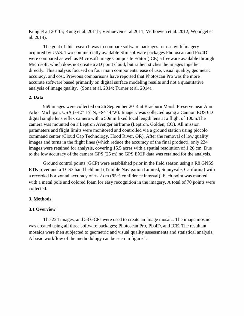
was used to parametrize each step (. A complete list of the parameters can be seen in table 1.

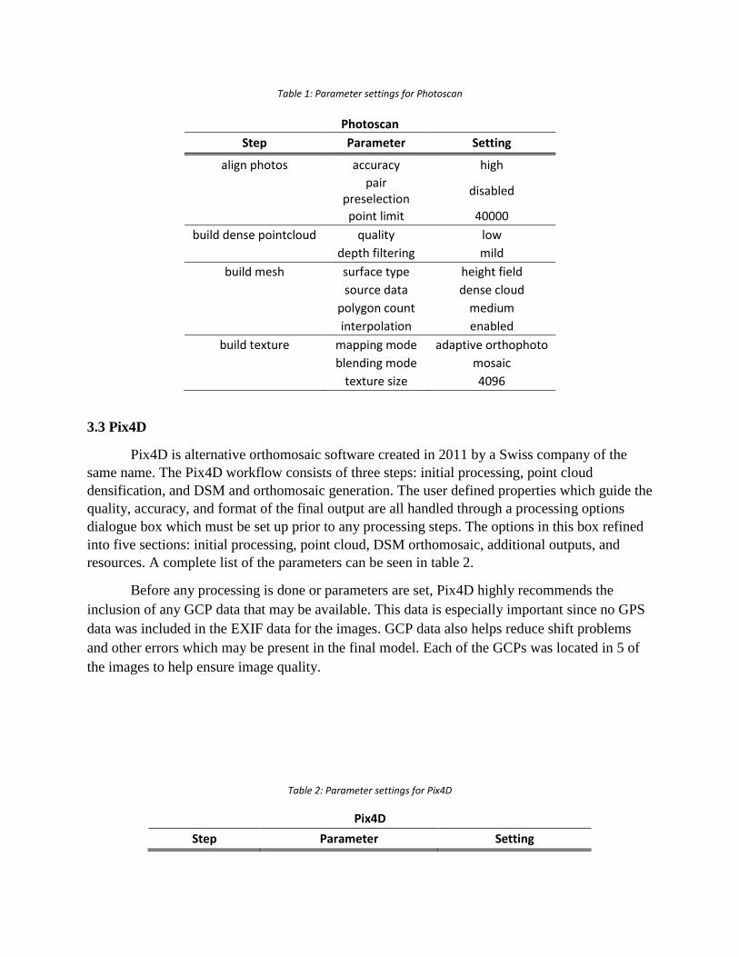
Table 1: Parameter settings for Photoscan

Photoscan

Step Parameter Setting

align photos accuracy high

pair

preselection disabled

point limit 40000

build dense pointcloud quality low

depth filtering mild

build mesh surface type height field

source data dense cloud

polygon count medium

interpolation enabled

build texture mapping mode adaptive orthophoto

blending mode mosaic

texture size 4096

3.3 Pix4D

Pix4D is alternative orthomosaic software created in 2011 by a Swiss company of the

same name. The Pix4D workflow consists of three steps: initial processing, point cloud

densification, and DSM and orthomosaic generation. The user defined properties which guide the

quality, accuracy, and format of the final output are all handled through a processing options

dialogue box which must be set up prior to any processing steps. The options in this box refined

into five sections: initial processing, point cloud, DSM orthomosaic, additional outputs, and

resources. A complete list of the parameters can be seen in table 2.

Before any processing is done or parameters are set, Pix4D highly recommends the

inclusion of any GCP data that may be available. This data is especially important since no GPS

data was included in the EXIF data for the images. GCP data also helps reduce shift problems

and other errors which may be present in the final model. Each of the GCPs was located in 5 of

the images to help ensure image quality.

Table 2: Parameter settings for Pix4D

Pix4D

Step Parameter Setting

initial processing processing aerial nadir

feature extraction 1

optimization externals and all internals

output none selected

point cloud image scale 1/4 (multiscale on)

point density optimal

minimum number of matches 3

point cloud filters none

DSM/orthomosaic noise filtering on

surface smoothing on

export type geotiff

resources resources all available

3.4 Microsoft ICE

ICE is an advanced panoramic image stitcher freeware produced by Microsoft typically

used to create detailed panoramas from numerous individual images. Unlike the other software

packages, ICE does not create a separate 3D point cloud and cannot generate 3D images. For

these reason, and because it is not designed to be used in scientific research, it does not create the

same number of outputs as Photoscan and Pix4D (i.e. no dense point clouds or

meshes).Therefore number of steps and parameters is relatively limited. In addition ICE

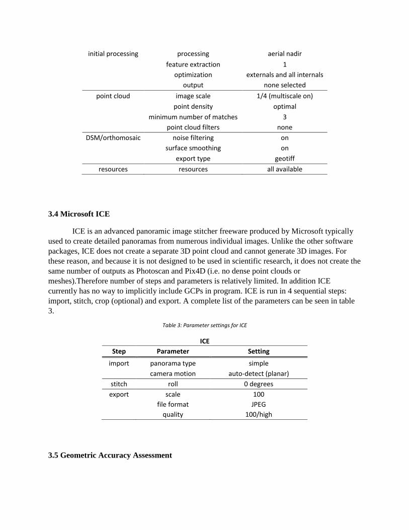
currently has no way to implicitly include GCPs in program. ICE is run in 4 sequential steps:

import, stitch, crop (optional) and export. A complete list of the parameters can be seen in table

3.

Table 3: Parameter settings for ICE

ICE

Step Parameter Setting

import panorama type simple

camera motion auto-detect (planar)

stitch roll 0 degrees

export scale 100

file format JPEG

quality 100/high

3.5 Geometric Accuracy Assessment

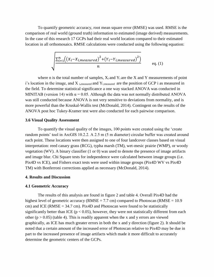
To quantify geometric accuracy, root mean square error (RMSE) was used. RMSE is the

comparison of real world (ground truth) information to estimated (image derived) measurements.

In the case of this research 17 GCPs had their real world location compared to their estimated

location in all orthomosaics. RMSE calculations were conducted using the following equation:

√∑ ((𝑋𝑖−𝑋𝑖,𝑚𝑒𝑎𝑠𝑢𝑟𝑒𝑑)

2+(𝑌𝑖−𝑌𝑖,𝑚𝑒𝑎𝑠𝑢𝑟𝑒𝑑)

2)𝑛

𝑖=1

𝑛 eq. (1)

where n is the total number of samples, Xi and Yi are the X and Y measurements of point

i’s location in the image, and X i,measured and Yi,measured are the position of GCP i as measured in

the field. To determine statistical significance a one way stacked ANOVA was conducted in

MINITAB (version 14) with α = 0.05. Although the data was not normally distributed ANOVA

was still conducted because ANOVA is not very sensitive to deviations from normality, and is

more powerful than the Kruskal-Wallis test (McDonald, 2014). Contingent on the results of the

ANOVA post hoc Tukey-Kramer test were also conducted for each pairwise comparison.

3.6 Visual Quality Assessment

To quantify the visual quality of the images, 100 points were created using the ‘create

random points’ tool in ArcGIS 10.2.2. A 2.5 m (5 m diameter) circular buffer was created around

each point. These locations were then assigned to one of four landcover classes based on visual

interpretation: reed canary grass (RCG), typha marsh (TM), wet-mesic prairie (WMP), or woody

vegetation (WV). A binary classifier (1 or 0) was used to denote the presence of image artifacts

and image blur. Chi Square tests for independence were calculated between image groups (i.e.

Pix4D vs ICE), and Fishers exact tests were used within image groups (Pix4D WV vs Pix4D

TM) with Bonferroni corrections applied as necessary (McDonald, 2014).

4. Results and Discussion

4.1 Geometric Accuracy

The results of this analysis are found in figure 2 and table 4. Overall Pix4D had the

highest level of geometric accuracy (RMSE = 7.7 cm) compared to Photoscan (RMSE = 10.9

cm) and ICE (RMSE = 34.7 cm). Pix4D and Photoscan were found to be statistically

significantly better than ICE (p < 0.05), however, they were not statistically different from each

other (p > 0.05) (table 4). This is readily apparent when the x and y errors are viewed

graphically, as ICE has much greater errors in both the x and y direction (figure 2). It should be

noted that a certain amount of the increased error of Photoscan relative to Pix4D may be due in

part to the increased presence of image artifacts which made it more difficult to accurately

determine the geometric centers of the GCPs.

The accuracies achieved by Photoscan Pro and Pix4d are comparable to values reported

in previous literature using UAS imagery. For example, a study conducted in 2010 by Laliberte

et al found RMSE values of 11.95 cm, 20.17 cm, and 16.69 cm for images collected over three

study sites in southwestern Idaho.

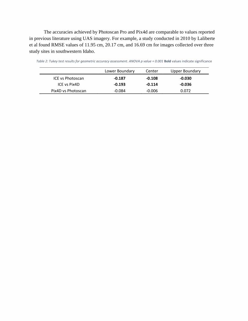
Table 2: Tukey test results for geometric accuracy assessment. ANOVA p value = 0.001 Bold values indicate significance

Lower Boundary Center Upper Boundary

ICE vs Photoscan -0.187 -0.108 -0.030

ICE vs Pix4D -0.193 -0.114 -0.036

Pix4D vs Photoscan -0.084 -0.006 0.072

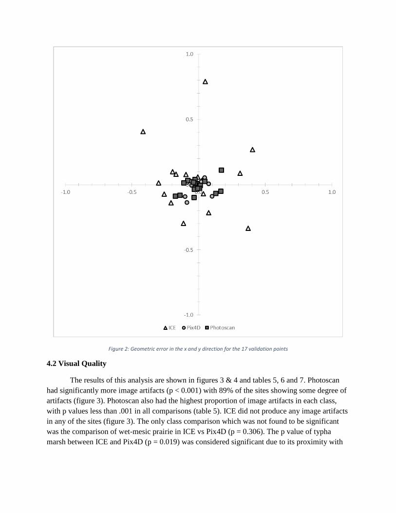
Figure 2: Geometric error in the x and y direction for the 17 validation points

4.2 Visual Quality

The results of this analysis are shown in figures 3 & 4 and tables 5, 6 and 7. Photoscan

had significantly more image artifacts (p < 0.001) with 89% of the sites showing some degree of

artifacts (figure 3). Photoscan also had the highest proportion of image artifacts in each class,

with p values less than .001 in all comparisons (table 5). ICE did not produce any image artifacts

in any of the sites (figure 3). The only class comparison which was not found to be significant

was the comparison of wet-mesic prairie in ICE vs Pix4D (p = 0.306). The p value of typha

marsh between ICE and Pix4D (p = 0.019) was considered significant due to its proximity with

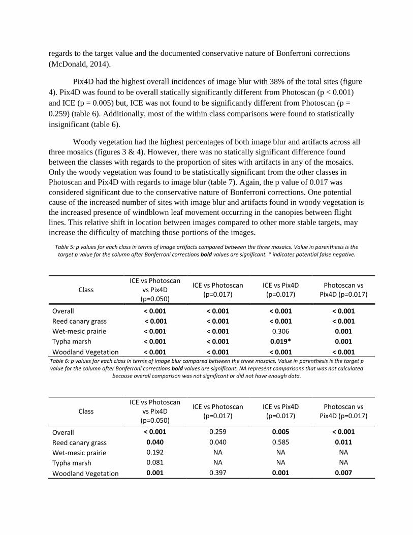
regards to the target value and the documented conservative nature of Bonferroni corrections

(McDonald, 2014).

Pix4D had the highest overall incidences of image blur with 38% of the total sites (figure

4). Pix4D was found to be overall statically significantly different from Photoscan (p < 0.001)

and ICE (p = 0.005) but, ICE was not found to be significantly different from Photoscan (p =

0.259) (table 6). Additionally, most of the within class comparisons were found to statistically

insignificant (table 6).

Woody vegetation had the highest percentages of both image blur and artifacts across all

three mosaics (figures 3 & 4). However, there was no statically significant difference found

between the classes with regards to the proportion of sites with artifacts in any of the mosaics.

Only the woody vegetation was found to be statistically significant from the other classes in

Photoscan and Pix4D with regards to image blur (table 7). Again, the p value of 0.017 was

considered significant due to the conservative nature of Bonferroni corrections. One potential

cause of the increased number of sites with image blur and artifacts found in woody vegetation is

the increased presence of windblown leaf movement occurring in the canopies between flight

lines. This relative shift in location between images compared to other more stable targets, may

increase the difficulty of matching those portions of the images.

Table 5: p values for each class in terms of image artifacts compared between the three mosaics. Value in parenthesis is the target p value for the column after Bonferroni corrections bold values are significant. * indicates potential false negative.

Class ICE vs Photoscan

vs Pix4D (p=0.050)

ICE vs Photoscan (p=0.017)

ICE vs Pix4D (p=0.017)

Photoscan vs Pix4D (p=0.017)

Overall < 0.001 < 0.001 < 0.001 < 0.001

Reed canary grass < 0.001 < 0.001 < 0.001 < 0.001

Wet-mesic prairie < 0.001 < 0.001 0.306 0.001

Typha marsh < 0.001 < 0.001 0.019* 0.001

Woodland Vegetation < 0.001 < 0.001 < 0.001 < 0.001 Table 6: p values for each class in terms of image blur compared between the three mosaics. Value in parenthesis is the target p value for the column after Bonferroni corrections bold values are significant. NA represent comparisons that was not calculated

because overall comparison was not significant or did not have enough data.

Class ICE vs Photoscan

vs Pix4D (p=0.050)

ICE vs Photoscan (p=0.017)

ICE vs Pix4D (p=0.017)

Photoscan vs Pix4D (p=0.017)

Overall < 0.001 0.259 0.005 < 0.001

Reed canary grass 0.040 0.040 0.585 0.011

Wet-mesic prairie 0.192 NA NA NA

Typha marsh 0.081 NA NA NA

Woodland Vegetation 0.001 0.397 0.001 0.007

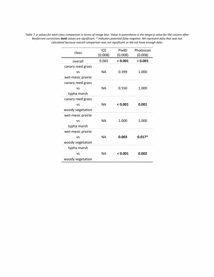
Table 7: p values for each class comparison in terms of image blur. Value in parenthesis is the target p value for the column after Bonferroni corrections bold values are significant. * indicates potential false negative. NA represent data that was not

calculated because overall comparison was not significant or did not have enough data.

class ICE

(0.008) Pix4D

(0.008) Photoscan

(0.008)

overall 0.065 < 0.001 < 0.001

canary reed grass

NA 0.399 1.000 vs

wet-mesic prairie

canary reed grass

NA 0.550 1.000 vs

typha marsh

canary reed grass

NA < 0.001 0.001 vs

woody vegetation

wet-mesic prairie

NA 1.000 1.000 vs

typha marsh

wet-mesic prairie

NA 0.003 0.017* vs

woody vegetation

typha marsh

NA < 0.001 0.002 vs

woody vegetation

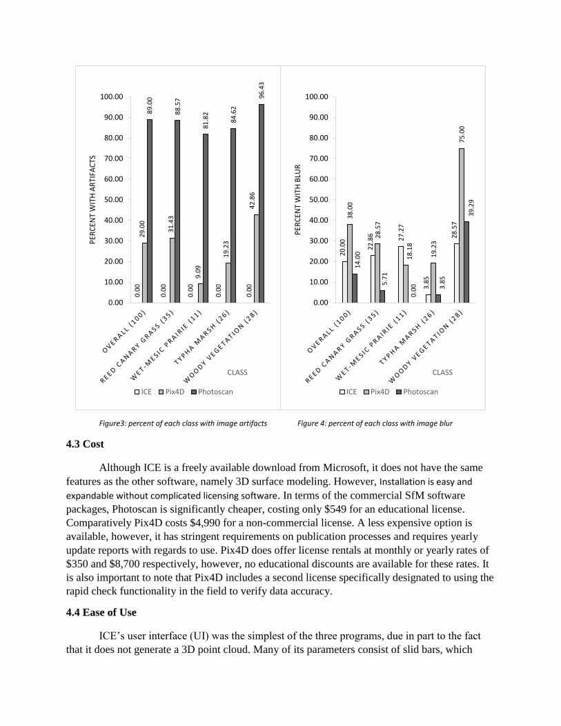
Figure3: percent of each class with image artifacts Figure 4: percent of each class with image blur

4.3 Cost

Although ICE is a freely available download from Microsoft, it does not have the same

features as the other software, namely 3D surface modeling. However, Installation is easy and

expandable without complicated licensing software. In terms of the commercial SfM software

packages, Photoscan is significantly cheaper, costing only $549 for an educational license.

Comparatively Pix4D costs $4,990 for a non-commercial license. A less expensive option is

available, however, it has stringent requirements on publication processes and requires yearly

update reports with regards to use. Pix4D does offer license rentals at monthly or yearly rates of

$350 and $8,700 respectively, however, no educational discounts are available for these rates. It

is also important to note that Pix4D includes a second license specifically designated to using the

rapid check functionality in the field to verify data accuracy.

4.4 Ease of Use

ICE’s user interface (UI) was the simplest of the three programs, due in part to the fact

that it does not generate a 3D point cloud. Many of its parameters consist of slid bars, which

0.0

0

0.0

0

0.0

0

0.0

0

0.0

0

29

.00

31

.43

9.0

9

19

.23

42

.86

89

.00

88

.57

81

.82

84

.62

96

.43

0.00

10.00

20.00

30.00

40.00

50.00

60.00

70.00

80.00

90.00

100.00P

ERC

ENT

WIT

H A

RTI

FAC

TS

CLASS

ICE Pix4D Photoscan

20

.00

22

.86

27

.27

3.8

5

28

.57

38

.00

28

.57

18

.18

19

.23

75

.00

14

.00

5.7

1

0.0

0 3.8

5

39

.29

0.00

10.00

20.00

30.00

40.00

50.00

60.00

70.00

80.00

90.00

100.00

PER

CEN

T W

ITH

BLU

R

CLASS

ICE Pix4D Photoscan

make adjustments simple. With only a single processing step, ICE offers the least amount of

control over the workflow. Additionally, it does not possess any in program GCP placement UI,

meaning that third party software such as ENVI or ArcGIS is required to georeference the

resulting mosaic.

Overall the UI of Photoscan was clean and user friendly. Images could be easily added,

disabled, and removed at any point in the workflow. Each step could be run and saved

independently making it much easier to adjust settings of individual steps to achieve the best

results. Multiple GCPs could be placed in one image at a time, and have their location predicted,

significantly reducing time and effort when placing GCPs, which is the most user intensive step

of the process. Photoscan also offers an easy to use batch processing mode, which allows users to

chain together any functionality, set parameters, and run them as one process.

Pix4D offered the most complicated UI. Included in its UI is a basemap image allowing

for an in program comparison of GCPs and mosaics to the real world prior to export.

Unfortunately, this can, at times, make viewing the finished mosaic in program slightly

cumbersome. In contrast to Photoscan’s modular setup, Pix4D has all its parameters set up in

advance using a single options menu. The initial processing, point cloud densification, and

DSM/Orthomosaic creation can then be run independently or all handled in a single execution.

Pix4D highly recommends the inclusion of GCP data not only to georeference the final outputs,

but also to help avoid a number of common errors, such as inverted mosaics. Pix4D’s UI for

GCP placement, however, uses small sub windows within the layout and requires significant

time and energy to implement (approx. 8 hours for 52 GCPs with 5 images each), compared to

Photoscan (approx. 4 hours).

5. Conclusion

With the use of UAS increasing both in the academic and civil sectors it is important to

find quick, accurate methods for converting significant numbers of images into a single usable

orthomosaic. This research has presented three possible alternative software packages which

offer a highly automated approach, Photoscan Pro, Pix4D, and Microsoft Image Composite

Editor. A summary of the findings can be seen in table 8. Although, Photoscan Pro and

Microsoft Image Composite Editor were easier to use than Pix4D, Photoscan proved to be least

effective in terms of visual accuracy, and ICE had the worst geometric accuracy. In addition all

three software packages struggled with tree canopies where windblown leaf movement led to

increased numbers of image artifacts or blur. Therefore, this research suggests that there is no

single best option for optimizing all criteria, and a software selection should reflect the

cost/benefit trade off between cost, ease of use, geometric accuracy, and visual quality for the

individual application.

Table8: Overall comparison between the software. Numbers represent the software order for that category with 1 being the highest. Duplicate values were awarded in cases where no statistical difference was observed

6. Acknowledgements and Funding

This research was funded by the Center for Geographic Information Science at Central Michigan

University. Without the help of Dr. Benjamin Heumann, Rachel Hackett, Brian Stark, and Sam Lipscomb

with regards to data collection this project would not have been possible. In addition, a special thanks is

given to Braeburn Nature Preserve for allowing us frequent access to the site.

7. References

Barazzetti, L., F. Remondino, M. Scaioni, and R. Brumana. 2010. Fully automatic UAV image-

based sensor orientation.in Proceedings of the 2010 Canadian Geomatics Conference and

Symposium of Commission I.

Choudhary, S., and P. Narayanan. 2012. Visibility probability structure from sfm datasets and

applications. Pages 130-143 Computer Vision–ECCV 2012. Springer.

DeGarmo, M. T. 2004. Issues concerning integration of unmanned aerial vehicles in civil

airspace. The MITRE Corporation Center for Advanced Aviation System Development.

Knoth, C., B. Klein, T. Prinz, and T. Kleinebecker. 2013. Unmanned aerial vehicles as

innovative remote sensing platforms for high‐resolution infrared imagery to support

restoration monitoring in cut‐over bogs. Applied Vegetation Science 16:509-517.

Küng, O., C. Strecha, A. Beyeler, J.-C. Zufferey, D. Floreano, P. Fua, and F. Gervaix. 2011a.

The accuracy of automatic photogrammetric techniques on ultra-light UAV imagery.in

UAV-g 2011-Unmanned Aerial Vehicle in Geomatics.

Küng, O., C. Strecha, P. Fua, D. Gurdan, M. Achtelik, K.-M. Doth, and J. Stumpf. 2011b.

Simplified building models extraction from ultra-light uav imagery. ISPRS-International

Archives of the Photogrammetry, Remote Sensing and Spatial Information Sciences

3822:217.

Laliberte, A. S., J. E. Herrick, A. Rango, and C. Winters. 2010. Acquisition, orthorectification,

and object-based classification of unmanned aerial vehicle (UAV) imagery for rangeland

monitoring. Photogrammetric Engineering & Remote Sensing 76:661-672.

Laliberte, A. S., A. Rango, and J. Herrick. 2007. Unmanned aerial vehicles for rangeland

mapping and monitoring: a comparison of two systems.in ASPRS Annual Conference

Proceedings.

Laliberte, A. S., C. Winters, and A. Rango. 2008. A procedure for orthorectification of sub-

decimeter resolution imagery obtained with an unmanned aerial vehicle (UAV). Pages

08-047 in Proc. ASPRS Annual Conf.

Geometric accuracy

Visual qualityCost

Ease of use

ICE 2 1 1 2

Photoscan Pro 1 3 2 1

Pix4D 1 2 3 3

Lindeberg, T. 2012. Scale invariant feature transform. Scholarpedia 7:10491.

Lowe, D. G. 2004. Distinctive image features from scale-invariant keypoints. International

journal of computer vision 60:91-110.

McDonald, J. H. 2009. Handbook of biological statistics. Sparky House Publishing Baltimore,

MD.

Sona, G., L. Pinto, D. Pagliari, D. Passoni, and R. Gini. 2014. Experimental analysis of different

software packages for orientation and digital surface modelling from UAV images. Earth

Science Informatics 7:97-107.

Turner, D., A. Lucieer, and L. Wallace. 2014. Direct georeferencing of ultrahigh-resolution uav

imagery.

Turner, D., A. Lucieer, and C. Watson. 2012. An automated technique for generating

georectified mosaics from ultra-high resolution unmanned aerial vehicle (UAV) imagery,

based on structure from motion (SfM) point clouds. Remote Sensing 4:1392-1410.

Verhoeven, G. 2011. Taking computer vision aloft–archaeological three‐dimensional

reconstructions from aerial photographs with photoscan. Archaeological Prospection

18:67-73.

Verhoeven, G., M. Doneus, C. Briese, and F. Vermeulen. 2012. Mapping by matching: a

computer vision-based approach to fast and accurate georeferencing of archaeological

aerial photographs. Journal of Archaeological Science 39:2060-2070.

Westoby, M., J. Brasington, N. Glasser, M. Hambrey, and J. Reynolds. 2012. ‘Structure-from-

Motion’photogrammetry: A low-cost, effective tool for geoscience applications.

Geomorphology 179:300-314.

Woodget, A., P. Carbonneau, F. Visser, and I. Maddock. 2014. Quantifying submerged fluvial

topography using hyperspatial resolution UAS imagery and structure from motion

photogrammetry. Earth Surface Processes and Landforms.

Zhang, Y., J. Xiong, and L. Hao. 2011. Photogrammetric processing of low‐altitude images

acquired by unpiloted aerial vehicles. The Photogrammetric Record 26:190-211.

Zhenkun, T., F. Yingying, and L. Suhong. 2013. Rapid crops classification based on UAV low-

altitude remote sensing. Transactions of the Chinese Society of Agricultural Engineering

2013.