Dynamic Systems and Applications 18 (2009) 483-506
TRIGONOMETRIC AND HYPERBOLIC SYSTEMS
ON TIME SCALES
R. HILSCHER AND P. ZEMANEK
Department of Mathematics and Statistics, Faculty of Science
Masaryk University, Kotlarska 2, CZ-61137 Brno, Czech Republic
ABSTRACT. In this paper we discuss trigonometric and hyperbolic systems on time scales.
These systems generalize and unify their corresponding continuous-time and discrete-time analo-
gies, namely the systems known in the literature as trigonometric and hyperbolic linear Hamiltonian
systems and discrete symplectic systems. We provide time scale matrix definitions of the usual
trigonometric and hyperbolic functions and show that many identities known from the basic calcu-
lus extend to this general setting, including the time scale differentiation of these functions.
AMS (MOS) Subject Classification. 34C99, 39A12
1. INTRODUCTION
In this paper we study trigonometric and hyperbolic systems on time scales and
properties of their solutions, the time scale matrix trigonometric functions Sin, Cos,
Tan, Cotan, and time scale matrix hyperbolic functions Sinh, Cosh, Tanh, Cotanh,
which are all properly defined in this work. The trigonometric and hyperbolic sys-
tems from this paper generalize and unify their corresponding continuous-time and
discrete-time analogies, namely the systems known in the literature as trigonometric
and hyperbolic linear Hamiltonian systems and discrete symplectic systems. More
precisely, the system of the form
(CTS) X ′ = Q(t) U, U ′ = −Q(t) X,
where t ∈ [a, b], X(t), U(t), and Q(t) are n × n matrices and additionally the matrix
Q(t) is symmetric for all t ∈ [a, b], is called a continuous trigonometric system (CTS).
Basic properties of this system can be found in [3, 20, 30].
The discrete analog of (CTS) has the form
(DTS) Xk+1 = PkXk + QkUk, Uk+1 = −QkXk + PkUk,
Received June 30, 2008 1056-2176 $15.00 c©Dynamic Publishers, Inc.
484 R. HILSCHER AND P. ZEMANEK
where we use the notation Xk := X(k), k ∈ [a, b] ∩ Z, Xk, Uk, Pk, Qk are n × n
matrices and, additionally, for all k ∈ [a, b] ∩ Z the following holds
P Tk Pk + QT
k Qk = I = PkPTk + QkQ
Tk ,(1.1)
P Tk Qk and PkQ
Tk are symmetric,(1.2)
and it is called a discrete trigonometric system (DTS). Basic properties of this system
can be found in [2, 6, 32].
In a similar way we can define the continuous hyperbolic system (CHS) as
(CHS) X ′ = Q(t) U, U ′ = Q(t) X,
where t ∈ [a, b], X(t), U(t) and Q(t) are n× n matrices and, additionally, the matrix
Q(t) is symmetric for all t ∈ [a, b]. The system of this form was studied in [22].
The discrete hyperbolic system (DHS) is defined as
(DHS) Xk+1 = PkXk + QkUk, Uk+1 = QkXk + PkUk,
where k ∈ [a, b] ∩ Z, Xk, Uk, Pk, Qk are n × n matrices and, in addition to (1.2),
P Tk Pk − QT
k Qk = I = PkPTk − QkQ
Tk
holds for k ∈ [a, b] ∩ Z. The reader can get acquainted with these systems in [19,32].
The conditions for the coefficient matrices are set in such a way so that the
considered system is Hamiltonian, resp. symplectic. That is, for the relevant matrices(
0 Q(t)
−Q(t) 0
),
(0 Q(t)
Q(t) 0
), resp.
(Pk Qk
−Qk Pk
),
(Pk Qk
Qk Pk
),
we have the identities
ST (t)J + JS(t) = 0, resp. STk JSk = J , where J =
(0 I
−I 0
).
The aim of this paper is to unify and generalize the theories of continuous and
discrete trigonometric systems, as well as the theories of continuous and discrete hy-
perbolic systems. This will be done within the theory of symplectic (or Hamiltonian)
systems on time scales T. We derive for general time scales T the same identities
which are known for the special cases of the continuous time T = R or the discrete
time T = Z.
In the continuous time case the study of elementary properties of scalar and
matrix trigonometric functions goes back to the paper [5] of Bohl and to the work
of Barrett, Etgen, Dosly, and Reid, see [3, 12–15, 20, 21, 30]. Discrete time scalar
and matrix trigonometric functions were studied by Anderson, Bohner, and Dosly
in [2,6–8], and more recently by Dosla, Dosly, Pechancova, and Skrabakova in [11,18].
Parallel considerations but for the hyperbolic systems, both continuous and discrete,

TRIGONOMETRIC AND HYPERBOLIC SYSTEMS 485
can be found in the work [19, 22, 32] by Dosly, Filakovsky, Pospısil, and the second
author. As for the general time scale setting, scalar trigonometric and hyperbolic
functions were defined in [9, Chapter 3] by Bohner and Peterson and in [27] by
Pospısil. Some properties of the matrix analogs of the time scale trigonometric and
hyperbolic functions were established in the papers [16,28,29] by Dosly and Pospısil.
By the same technique as in [14], namely considering two different systems with
the same initial conditions, we establish additive and difference formulas for trigono-
metric and hyperbolic systems on time scales. In particular, utilizing these identities
in the continuous time we derive n-dimensional analogies of many classical formulas
which are known for trigonometric and hyperbolic systems in the scalar case. The
second purpose of this paper is to provide a concise but complete treatment of prop-
erties of time scale matrix trigonometric and hyperbolic functions, as well as to point
out to the analogies between them.
The setup of this paper is the following. In the next section we collect preliminary
properties of time scales and time scale symplectic systems which will be needed
throughout the paper. In Section 3 we present the theory and new formulas for the
trigonometric systems on time scales. Similar results are then derived in Section 4 for
the hyperbolic systems on time scales. Finally, in Section 5 we discuss the difficulties
which arise in extending some of the scalar addition formulas to time scales.
We remark, that we present all results in the real case (i.e., for the real-valued
coefficients and solutions), but they hold in the complex domain as well. For this we
only need to replace the transpose of a matrix by the conjugate transpose, the term
“symmetric” by “Hermitian”, and “orthogonal” by “unitary”. Note also that all our
results hold on arbitrary infinite (continuous, discrete, or time scale) intervals. This
fact is important for the future possible development of the oscillation theory of the
trigonometric and hyperbolic systems.
2. PRELIMINARIES ON TIME SCALES AND
SYMPLECTIC SYSTEMS
In this section we introduce basic concepts, notations, and fundamental properties
of time scales and time scale symplectic systems. The founder of the time scale theory
is Stefan Hilger who established in [23] the calculus of time scales or measure chains.
The monographs [9] and [10] offer extended knowledge of this theory.
By definition, a time scale T is any nonempty closed subset of the real numbers
R. In this paper we will consider a bounded time scale T which can therefore be
identified with the time scale interval [a, b]T := [a, b] ∩ T, where a := min T and
b := max T, and where [a, b] is the usual interval of real numbers. Similarly, we use
the notation [a, b]Z for a discrete interval with a, b ∈ Z, i.e., [a, b]Z := [a, b]∩Z. Open
and half-open time scale intervals are defined accordingly.

486 R. HILSCHER AND P. ZEMANEK
The forward jump operator σ : T → T is defined by σ(t) := inf{s ∈ T | s > t}
(and simultaneously we put inf ∅ := sup T). The backward jump operator ρ : T → T is
defined by ρ(t) := sup{s ∈ T | s < t} (simultaneously we put sup ∅ := inf T). A point
t ∈ (a, b]T is said to be left-dense if ρ(t) = t, while a point t ∈ [a, b)T right-dense if
σ(t) = t. Also a point t ∈ [a, b]T is left-scattered, resp. right-scattered if ρ(t) < t, resp.
σ(t) > t. The graininess function µ : T → [0,∞) is defined by µ(t) := σ(t) − t.
For a function f on [a, ρ(b)]T the time scale derivative f∆(t) is defined in such
a way that it reduces to the usual derivative f ′(t) at every right-dense point t (in
particular, in the continuous time at all t), and it reduces to the forward difference
∆f(t) = f(t + 1)− f(t) at every right-scattered point t (in particular, in the discrete
time at all t). In addition, if T = R, then σ(t) = t = ρ(t) and µ(t) ≡ 0, while if
T = Z, then σ(t) = t +1, ρ(t) = t− 1, and µ(t) ≡ 1. For brevity, we use the notation
fσ(t) := f(σ(t)) and f ρ(t) := f(ρ(t)).
A function f : [a, b]T → R is said to be rd-continuous (f ∈ Crd) if it is continuous
at each right-dense point and there exists a finite left-hand limit at each left-dense
point. A function f is said to be rd-continuously ∆-differentiable (f ∈ C1rd) if f∆
exists on [a, ρ(b)]T and f∆ ∈ Crd. Note that if f∆(t) exists, then
(2.1) fσ(t) = f(t) + µ(t) f∆(t).
If b is a left-scattered point, then f∆(b) is not well-defined. The usual differential rules
take in this case the form (f ± g)∆(t) = f∆(t) ± g∆(t) and (fg)∆(t) = f∆(t) g(t) +
fσ(t) g∆(t). The time scale integral is defined accordingly but it will not be used in
this paper.
A matrix function A : [a, ρ(b)]T → Rn×n is said to be regressive on an interval
J ⊆ [a, ρ(b)]T if the matrix I + µ(t) A(t) is invertible for all t ∈ J . It is known, see
e.g. [23, Theorem 5.7], that if A ∈ Crd and A is regressive on [a, t0)T, then the initial
value problem
z∆ = A(t) z, t ∈ [a, ρ(b)]T, z(t0) = z0,
has a unique solution z(t) on [a, b]T for any t0 ∈ [a, b]T and any z0. Observe that the
regressivity assumption is void if t0 = a.
Let A be a differentiable n×n matrix-valued function such that AAσ is invertible.
Then the differentiation of the identity AA−1 = I yields
(2.2) (A−1)∆ = −(Aσ)−1A∆ A−1 = −A−1A∆(Aσ)−1.
The time scale symplectic (or Hamiltonian) system is the first order linear system
(S) X∆ = A(t) X + B(t) U, U∆ = C(t) X + D(t) U,
TRIGONOMETRIC AND HYPERBOLIC SYSTEMS 487
where X, U : [a, b]T → Rn×n, the coefficients A,B, C,D ∈ Crd(R
n×n) on [a, ρ(b)]T, and
the matrix S(t) :=(A(t) B(t)C(t) D(t)
)satisfies
(2.3) ST (t)J + JS(t) + µ(t)ST (t)JS(t) = 0 on [a, ρ(b)]T.
This identity implies that the matrix I +µ(t)S(t) is symplectic. Recall that a 2n×2n
matrix M is symplectic if MTJM = J . Basic references for time scale symplectic
systems are [17, 25].
Since every symplectic matrix is invertible, it follows that the matrix function S
is regressive on [a, ρ(b)]T. Therefore, the initial value problems associated with (S)
have unique solutions for any initial point t0 ∈ [a, b]T and any (vector or matrix)
initial values, see also [9, Corollary 7.12].
If T = R, then with A(t) := A(t), B(t) := B(t), and C(t) := C(t) the system (S)
is the linear Hamiltonian system (see e.g. [26] or [31])
X ′ = A(t) X + B(t) U, U ′ = C(t) X − AT (t) U,
where the matrix S(t) :=(
A(t) B(t)
C(t) −AT (t)
)satisfies J S(t) + ST (t)J = 0 for all t ∈ [a, b],
i.e., the matrix S(t) is Hamiltonian. If T = Z, then with Ak := I +A(k), Bk := B(k),
Ck := C(k), and Dk := I +D(k) the system (S) is the discrete symplectic system (see
e.g. [1, 32])
Xk+1 = AkXk + BkUk, Uk+1 = CkXk + DkUk,
where the matrix Sk :=(Ak Bk
Ck Dk
)is symplectic.
In the block notation identity (2.3) is equivalent to (we omit the argument t)
BT − B + µ (BTD −DTB) = 0,
CT − C + µ (CTA−ATC) = 0,
AT + D + µ (ATD − CTB) = 0.
This implies that the matrices BT (I +µD) and CT (I +µA) are symmetric. Note that
other equivalent identities are derived in [10, Remark 10.1] by using the fact that
I + µ(t)ST (t) is symplectic. But these identities are not used in this paper.
If Z = (XU) and Z =
(XU
)are any solutions of (S), then their Wronskian matrix
is defined on [a, b]T as W (Z, Z)(t) := XT (t) U(t) − UT (t) X(t). The following is a
simple consequence of W∆(Z, Z)(t) ≡ 0.
Proposition 2.1. Let Z = (XU) and Z =
(XU
)be any solutions of (S). Then the
Wronskian W (Z, Z)(t) ≡ W is constant on [a, b]T.
A solution Z = (XU) of (S) is said to be a conjoined solution if W (Z, Z) ≡ 0, i.e.,
XT U is symmetric at one and hence at any t ∈ [a, b]T. Two solutions Z and Z are
normalized if W (Z, Z) ≡ I. A solution Z and is said to be a basis if rank Z(t) ≡ n

488 R. HILSCHER AND P. ZEMANEK
on [a, b]T. It is known that for any conjoined basis Z there always exists another
conjoined basis Z such that Z and Z are normalized (see [9, Lemma 7.29]).
Proposition 2.2. Let Z be any solution of (S). Then rank Z(t) ≡ r is constant on
[a, b]T.
Proof. Let Φ(t) be a fundamental matrix of system (S), i.e., Φ = (Z, Z), where Z and
Z are normalized. Then every solution of (S) is a constant multiple of Φ(t), that is,
Z(t) = Φ(t) M on [a, b]T for some M ∈ R2n×n. If rank Z(t0) = r at some t0 ∈ [a, b]T,
then rankM = r. Consequently, rankZ(t) = r for all t ∈ [a, b]T.
From Propositions 2.1 and 2.2 we can see that the defining properties of conjoined
bases of (S) can be prescribed just at one point t0 ∈ [a, b]T, for example by the initial
condition Z(t0) = Z0 with ZT0 JZ0 = 0 and rankZ0 = n.
Proposition 2.3. Two solutions Z and Z of system (S) are normalized conjoined
bases if and only if the 2n × 2n matrix Φ(t) := (Z(t), Z(t)) is symplectic for all
t ∈ [a, b]T.
The proof is straightforward and can be found e.g. in [9, Lemma 7.27]. It follows
that Z = (XU) and Z =
(XU
)are normalized conjoined bases if and only if
(2.4)
{XT U − UT X = I = XUT − UXT ,
XT U = UT X, XT U = UT X, XXT = XXT , UUT = UUT .
The fact that the matrix Φ is symplectic for all t ∈ [a, b]T implies that Φ−1 = J T ΦTJ ,
and thus from Φσ = (I + µS) Φ we get ΦσJ T ΦTJ = I + µS. That is,
(2.5)
XσUT − XσUT = I + µA, XσXT − XσXT = µB,
UσXT − UσXT = I + µD, UσUT − UσUT = µC.
For a given point t0 ∈ [a, b]T, the conjoined basis(
XU
)of (S) determined by the
initial conditions X(t0) = 0 and U(t0) = I is called the principal solution at t0.
3. TIME SCALE TRIGONOMETRIC SYSTEMS
In this section we consider the system (S), where the matrix S(t) takes the form
S(t) =(
P(t) Q(t)−Q(t) P(t)
), where P,Q ∈ Crd(R
n×n) on [a, ρ(b)]T. Therefore, from (2.3) we
get that the matrices P and Q satisfy the identities (we omit the argument t)
QT −Q + µ (QTP − PTQ) = 0,(3.1)
PT + P + µ (QTQ + PTP) = 0(3.2)
for all t ∈ [a, ρ(b)]T, see also [9, pg. 312] and [24, Theorem 7].

TRIGONOMETRIC AND HYPERBOLIC SYSTEMS 489
Definition 3.1 (Time scale trigonometric system). The system
(TTS) X∆ = P(t) X + Q(t) U, U∆ = −Q(t) X + P(t) U,
where the coefficient matrices satisfy identities (3.1) and (3.2) for all t ∈ [a, ρ(b)]T, is
called a time scale trigonometric system (TTS).
Remark 3.2. System (S) is trigonometric if its coefficients satisfy, in addition to
(2.3) the identity J TS(t)J = S(t) for all t ∈ [a, ρ(b)]T. Therefore, trigonometric
systems are also called self-reciprocal, see [9, Definition 7.50].
Remark 3.3. Now, we compare the continuous time trigonometric system arising
from Definition 3.1, with the system (CTS) introduced in Section 1. For [a, b]T = [a, b],
the system (TTS) from Definition 3.1 takes the form
(3.3) X ′ = P(t) X + Q(t) U, U ′ = −Q(t) X + P(t) U,
where Q(t) is symmetric and P(t) is antisymmetric, see (3.1) and (3.2) with µ = 0.
Now we use the special transformation to reduce the system (3.3) into (CTS), see
[8, 30].
More precisely, let H(t) be a solution of the system H ′ = P(t) H with the initial
condition HT (a) H(a) = I, i.e., the matrix H(a) is orthogonal. Now, we consider the
transformation X := H−1(t) X and U := HT (t) U , which yields
X ′ = H−1(t)Q(t) HT−1(t) U , U ′ = −HT (t)Q(t) H(t) X.
Hence, this resulting system will be of the form (CTS) once we show that HT (t) =
H−1(t) for all t ∈ [a, b]. But this follows from the calculation (HT H)′ = 0 and
from the initial condition on H(a). Now, we put Q(t) := HT (t)Q(t) H(t) which is
symmetric, so that
X ′ = Q(t) U , U ′ = −Q(t) X.
Remark 3.4. Now we consider the discrete case and show that the time scale trigono-
metric system (TTS) reduces for [a, b]T = [a, b]Z to the system (DTS) introduced in
Section 1. Upon setting Pk := I + P(k) and Qk := Q(k) one can easily see that
identities (3.1) and (3.2) are in this case equivalent to the properties of Pk and Qk in
(1.1)–(1.2).
Now we turn our attention to solutions of the general time scale trigonometric
system.
Lemma 3.5. The pair (XU) solves the trigonometric system (TTS) if and only if the
pair(
U−X
)solves the same system. Equivalently (U
X) solves (TTS) if and only if(−X
U
)
does so.

490 R. HILSCHER AND P. ZEMANEK
The following definition extend to time scales the matrix sine and cosine functions
known in the continuous time in [3, pg. 511] and in the discrete case in [2, pg. 39].
Definition 3.6. Let s ∈ [a, b]T be fixed. We define the n×n matrix-valued functions
sine (denoted by Sins) and cosine (denoted by Coss) by
Sins(t) := X(t), Coss(t) := U(t),
where the pair (XU) is the principal solution of system (TTS) at s, that is, it is given
by the initial conditions X(s) = 0 and U(s) = I. We suppress the index s when
s = a, i.e., we denote Sin := Sina and Cos := Cosa.
Remark 3.7. (i) The matrix functions Sins and Coss are n-dimensional analogs of
the scalar trigonometric functions sin(t − s) and cos(t − s).
(ii) When n = 1 and P = 0 and Q = p with p ∈ Crd, the matrix functions Sins(t)
and Coss(t) reduce exactly to the scalar time scale trigonometric functions sinp(t, s)
and cosp(t, s) from [9, Definition 3.25].
(iii) In the continuous time scalar case and when P = 0, i.e., system (TTS) is
the same as (CTS), the solutions Sin(t) = sin∫ t
aQ(τ) dτ and Cos(t) = cos
∫ t
aQ(τ) dτ .
Similar formulas hold for the discrete scalar case, see [2, pg. 40].
Remark 3.8. By using Lemma 3.5, the above matrix sine and cosine functions can
be alternatively defined as Coss(t) := X(t) and Sins(t) := −U (t), where(
XU
)is the
solution of system (TTS) with the initial conditions X(s) = I and U(s) = 0.
By definition, the Wronskian of the two solutions (CosSin) and
(−Sin
Cos
)is W (t) ≡
W (a) = I. Hence, (CosSin) and
(− Sin
Cos
)form normalized conjoined bases of the system
(TTS) and
(3.4) Φ(t) :=
(Cos(t) − Sin(t)
Sin(t) Cos(t)
)
is a fundamental matrix of (TTS). Therefore, every solution (XU) of (TTS) has the
form
X(t) = Cos(t) X(a) − Sin(t) U(a) and U(t) = Sin(t) X(a) + Cos(t) U(a)
for all t ∈ [a, b]T. As a consequence of formulas (2.4) and (2.5) we get the following.
Corollary 3.9. For all t ∈ [a, b]T the identities
CosT Cos + SinT Sin = I = Cos CosT + Sin SinT ,(3.5)
CosT Sin = SinT Cos, Cos SinT = Sin CosT(3.6)
hold, while for all t ∈ [a, ρ(b)]T we have the identities
Cosσ CosT + Sinσ SinT = I + µP, Cosσ SinT − Sinσ CosT = µQ.
TRIGONOMETRIC AND HYPERBOLIC SYSTEMS 491
The following result is a matrix analog of the fundamental formula cos2(t) +
sin2(t) = 1 for scalar continuous time trigonometric functions, see also [9, Exer-
cise 3.30]. Here ‖·‖F is the usual Frobenius norm, i.e., ‖V ‖F =(∑n
i,j=1 v2ij
) 1
2 , see [4,
pg. 346].
Corollary 3.10. For all t ∈ [a, b]T we have the identity
(3.7) ‖Cos‖2F + ‖Sin‖2
F = n.
Proof. Since for arbitrary matrix V ∈ Rn×n the identity tr(V T V ) = ‖V ‖2
F holds,
equation (3.7) follows directly from (3.5).
Corollary 3.11. For all t ∈ [a, ρ(b)]T we have
Cos∆ CosT + Sin∆ SinT = P,(3.8)
Sin∆ CosT −Cos∆ SinT = Q.(3.9)
Proof. Since (SinCos) is the solution of system (TTS), we have Sin∆ = P Sin +QCos and
Cos∆ = −Q Sin +P Cos. If we now multiply the first of these two identities by the
matrix SinT from the right and the second one by CosT from the right, and if we
add the two obtained equations, then formula (3.8) follows. In these computations
we also used the second identities from (3.5) and (3.6). Similar calculations lead to
formula (3.9).
Remark 3.12. If the matrix Cos and/or Sin is invertible at some point t ∈ [a, b]T,
then, by (3.5) and (3.6), we can write
(3.10) Cos−1 = CosT + SinT CosT−1 SinT , Sin−1 = SinT + CosT SinT−1 CosT .
Next we present additive formulae for matrix trigonometric functions on time
scales. This result generalizes its continuous time counterpart in [21, Theorem 1.1]
to time scales.
Theorem 3.13. For t, s ∈ [a, b]T we have
Sins(t) = Sin(t) CosT (s) − Cos(t) SinT (s),(3.11)
Coss(t) = Cos(t) CosT (s) + Sin(t) SinT (s),(3.12)
Sin(t) = Sins(t) Cos(s) + Coss(t) Sin(s),(3.13)
Cos(t) = Coss(t) Cos(s) − Sins(t) Sin(s).(3.14)
Proof. We set
V (t) := Sin(t) CosT (s) − Cos(t) SinT (s), Y (t) := Cos(t) CosT (s) + Sin(t) SinT (s).

492 R. HILSCHER AND P. ZEMANEK
Then we calculate
V ∆(t) = Sin∆(t) CosT (s) − Cos∆(t) SinT (s) = P(t)V (t) + Q(t)Y (t),
Y ∆(t) = Cos∆(t) CosT (s) + Sin∆(t) SinT (s) = −Q(t)V (t) + P(t)Y (t),
where we used the second identities from (3.5) and (3.6) at t. The initial values are
V (s) = 0 and Y (s) = I, where we used the second identities from (3.5) and (3.6)
at s. Hence, equations (3.11) and (3.12) follow from the uniqueness of solutions of
time scale symplectic systems. That is V (t) = Sins(t) and Y (t) = Coss(t). Note that
equations (3.11) and (3.12) can be written as
(3.15)(Sins(t) Coss(t)
)=(Sin(t) Cos(t)
)( CosT (s) SinT (s)
− SinT (s) CosT (s)
),
where the 2n × 2n matrix on the right-hand side equals to Φ−1(s) and the matrix
Φ(s) is defined in (3.4). Multiplying equality (3.15) by Φ(s) from the right, identities
(3.13) and (3.14) follow.
With respect to Remark 3.7 for the scalar continuous time case, identities (3.11)–
(3.14) are matrix analogies of elementary trigonometric identities.
Interchanging the parameters t and s in (3.11) and (3.12) yields expected prop-
erties of the matrix trigonometric functions.
Corollary 3.14. Let t, s ∈ [a, b]T. Then
(3.16) Sins(t) = − SinTt (s) and Coss(t) = CosT
t (s).
Remark 3.15. In the scalar continuous time case and when Q(t) ≡ 1 the formulas in
(3.16) have the form sin(t−s) = − sin(s−t) and cos(t−s) = cos(s−t). Consequently, if
we let s = 0, we obtain sin(t) = − sin(−t) and cos(t) = cos(−t), so that Corollary 3.14
is the matrix analogue of the statement about the parity for the scalar functions sine
and cosine.
Next we wish to generalize the sum and difference formulae for solutions of two
time scale symplectic systems. This can be done via the approach from [14]. This
leads to a generalization of several formulas known in the scalar continuous case.
Observe that, comparing to Theorem 3.13 in which we consider one system and
solutions with different initial conditions, we shall now deal with two systems and
solutions with the same initial conditions. Consider the following two time scale
trigonometric systems
(3.17) X∆ = P(i)(t) X + Q(i)(t) U, U∆ = −Q(i)(t) X + P(i)(t) U
with initial conditions X(i)(a) = 0 and U(i)(a) = I, where i = 1, 2. Denote by Sin(i)(t)
and Cos(i)(t) the corresponding matrix sine and cosine functions from Definition 3.6.

TRIGONOMETRIC AND HYPERBOLIC SYSTEMS 493
Put
Sin±(t) := Sin(1)(t) CosT(2)(t) ± Cos(1)(t) SinT
(2)(t),(3.18)
Cos±(t) := Cos(1)(t) CosT(2)(t) ∓ Sin(1)(t) SinT
(2)(t).(3.19)
Theorem 3.16. Assume that P(i) and Q(i) satisfy (3.1) and (3.2). The pair Sin± and
Cos± solves the system
(3.20)
X∆ = P(1)X + Q(1)U + XPT(2) ± UQT
(2)
+ µ [P(1) (XPT(2) ± UQT
(2)) + Q(1) (∓XQT(2) + UPT
(2))],
U∆ = −Q(1)X + P(1)U ∓ XQT(2) + UPT
(2)
+ µ [−Q(1) (XPT(2) ± UQT
(2)) + P(1) (∓XQT(2) + UPT
(2))]
with the initial conditions X(a) = 0 and U(a) = I. Moreover, for all t ∈ [a, b]T we
have
Sin± (Sin±)T + Cos± (Cos±)T = I = (Sin±)T Sin± + (Cos±)T Cos±,(3.21)
Sin± (Cos±)T = Cos± (Sin±)T , (Sin±)T Cos± = (Cos±)T Sin± .(3.22)
Proof. All the statements in this theorem are proven by straightforward calculations.
In these we use the identities, see (2.1),
Sinσ(1) = Sin(1) +µ Sin∆
(1) = Sin(1) +µ (P(1) Sin(1) +Q(1) Cos(1)),
Cosσ(1) = Cos(1) +µ Cos∆
(1) = Cos(1) +µ (−Q(1) Sin(1) +P(1) Cos(1)),
the time scale product rule, and system (3.17) for i = 1, 2. Then it follows that the
pair Sin± and Cos± solves the system (3.20) and Sin±(a) = 0, Cos±(a) = I.
Next we show identity (3.21). From the definition of Sin+ and Cos+, from the
first identity in (3.5) for i = 1, and from the second identity in (3.6) for i = 2 we get
Sin+ (Sin+)T + Cos+ (Cos+)T = Sin(1) (CosT(2) Cos(2) + SinT
(2) Sin(2)) SinT(1)
+ Cos(1) (CosT(2) Cos(2) + SinT
(2) Sin(2)) CosT(1)
= Cos(1) CosT(1) + Sin(1) SinT
(1) = I.
The other identities in (3.21) are shown in analogous way. Similarly, by using (3.5)
and (3.6) for i = 1, 2 one can show that all the identities in (3.22) hold true.
Remark 3.17. The properties in (3.21) and (3.22) of solutions Sin± and Cos± of
system (3.20) mirror the properties in (3.5) and (3.6) of normalized conjoined bases
of (S). However, the two pairs(
Sin+
Cos+
)and
(Sin−
Cos−
)are not conjoined bases of their
corresponding systems, because these systems are not symplectic.
Remark 3.18. In the continuous time case the assertion of Theorem 3.16 is proven
in [14, Theorem 1]. On the other hand, the discrete form is new. The details can be
found in [33, Theorem 3.14].
494 R. HILSCHER AND P. ZEMANEK
When the two systems in (3.17) are the same, Theorem 3.16 yields the following.
Corollary 3.19. Assume that P and Q satisfy (3.1) and (3.2). Then the system
X∆ = PX + QU + XPT + UQT + µ [P (XPT + UQT ) + Q (−XQT + UPT )],
U∆ = −QX + PU − XQT + UPT + µ [−Q (XPT + UQT ) + P (−XQT + UPT )]
with the initial conditions X(a) = 0 and U(a) = I possesses the solution
X = 2 Sin CosT and U = Cos CosT − Sin SinT ,
where Sin and Cos are the matrix functions in Definition 3.6. Moreover, the above
matrices X and U commute, i.e., XU = UX.
Proof. The statement follows from Theorem 3.16 in which we take P(1) = P(2) = P,
Q(1) = Q(2) = Q, and Sin(1) = Sin(2) = Sin, Cos(1) = Cos(2) = Cos. Finally, from
(3.5) and (3.6) we get that XU − UX = 0.
The previous corollary can be viewed as the n-dimensional analogy of the double
angle formulae for scalar continuous time trigonometric functions. In the continuous
time case, the content of Corollary 3.19 is [20, Theorem 1.1]. On the other hand,
in the discrete case this result is new, see [33, Corollary 3.16]. The details are here
omitted.
Corollary 3.20. For all t ∈ [a, b]T we have the identities
Sin(1) SinT(2) =
1
2(Cos−−Cos+),(3.23)
Cos(1) CosT(2) =
1
2(Cos− + Cos+),(3.24)
Sin(1) CosT(2) =
1
2(Sin− + Sin+).(3.25)
Proof. Subtracting the two equations in (3.19) we obtain Cos− −Cos+ = 2 Sin(1) SinT(2)
from which formula (3.23) follows. Similarly, we have Cos− + Cos+ = 2 Cos(1) CosT(2)
and Sin− + Sin+ = 2 Sin(1) CosT(2) from which we get (3.24) and (3.25).
In the scalar continuous time case, identities (3.23)–(3.25) have the form of ele-
mentary trigonometric identities. The next definition is a natural time scale matrix
extension of the scalar trigonometric tangent and cotangent functions. It extends the
discrete matrix tangent and cotangent functions known in [2, pg. 42] to time scales.
Definition 3.21. Whenever Cos(t), resp. Sin(t), is invertible we define the matrix-
valued function tangent (we write Tan), resp. cotangent (we write Cotan), by
Tan(t) := Cos−1(t) Sin(t), resp. Cotan(t) := Sin−1(t) Cos(t).
TRIGONOMETRIC AND HYPERBOLIC SYSTEMS 495
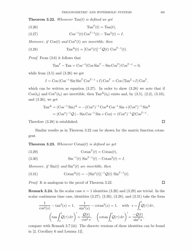
Theorem 3.22. Whenever Tan(t) is defined we get
TanT (t) = Tan(t),(3.26)
Cos−1(t) CosT−1(t) − Tan2(t) = I.(3.27)
Moreover, if Cos(t) and Cosσ(t) are invertible, then
(3.28) Tan∆(t) = [Cosσ(t)]−1Q(t) CosT−1(t).
Proof. From (3.6) it follows that
TanT −Tan = Cos−1(Cos SinT − Sin CosT ) CosT−1 = 0,
while from (3.5) and (3.26) we get
I = Cos (Cos−1 Sin SinT CosT−1 +I) CosT = Cos (Tan2 +I) CosT ,
which can be written as equation (3.27). In order to show (3.28) we note that if
Cos(t0) and Cosσ(t0) are invertible, then Tan∆(t0) exists and, by (3.5), (2.2), (3.10),
and (3.26), we get
Tan∆ = (Cos−1 Sin)∆ = −(Cosσ)−1 Cos∆ Cos−1 Sin +(Cosσ)−1 Sin∆
= (Cosσ)−1Q (− Sin Cos−1 Sin + Cos) = (Cosσ)−1QCosT−1 .
Therefore (3.28) is established.
Similar results as in Theorem 3.22 can be shown for the matrix function cotan-
gent.
Theorem 3.23. Whenever Cotan(t) is defined we get
CotanT (t) = Cotan(t),(3.29)
Sin−1(t) SinT−1(t) − Cotan2(t) = I.(3.30)
Moreover, if Sin(t) and Sinσ(t) are invertible, then
(3.31) Cotan∆(t) = −[Sinσ(t)]−1Q(t) SinT−1(t).
Proof. It is analogous to the proof of Theorem 3.22.
Remark 3.24. In the scalar case n = 1 identities (3.26) and (3.29) are trivial. In the
scalar continuous time case, identities (3.27), (3.30), (3.28), and (3.31) take the form
1
cos2(s)− tan2(s) = 1,
1
sin2(s)− cotan2(s) = 1, with s =
∫ t
a
Q(τ) dτ ,
(tan
∫ t
a
Q(τ) dτ
)′
=Q(t)
cos2 s,
(cotan
∫ t
a
Q(τ) dτ
)′
=−Q(t)
sin2 s,
compare with Remark 3.7 (iii). The discrete versions of these identities can be found
in [2, Corollary 6 and Lemma 12].

496 R. HILSCHER AND P. ZEMANEK
Remark 3.25. In the continuous time case with Q(t) ≡ I, i.e., when system (CTS)
is X ′ = U , U ′ = −X and hence it represents the second order matrix equation
X ′′ + X = 0, the matrix functions Sin, Cos, Tan, and Cotan satisfy
Sin′ = Cos, Cos′ = − Sin, Tan′ = Cos−1 CosT−1, Cotan′ = − Sin−1 SinT−1 .
The first two equalities follow from the definition of Sin and Cos, while the last two
equalities are simple consequences of (3.28) and (3.31).
Next, similarly to the definitions of the time scale matrix functions Sin(i), Cos(i),
Sin±, and Cos± from (3.17)–(3.19) we define the following functions
Tan(i)(t) := Cos−1(i) (t) Sin(i)(t), Cotan(i)(t) := Sin−1
(i) (t) Cos(i)(t),
Tan±(t) := [Cos±(t)]−1 Sin±(t), Cotan±(t) := [Sin±(t)]−1 Cos±(t).
Remark 3.26. It is natural that the matrix-valued functions Tan± have similar
properties as the function Tan. In particular, the first identity in (3.22) implies that
Tan± are symmetric. Similarly, the functions Cotan± are also symmetric.
The results of the following theorem are new even in the special case of continuous
and discrete time, see [33, Theorem 3.26].
Theorem 3.27. For all t ∈ [a, b]T such that all involved functions are defined we
have (suppressing the argument t)
Tan(1) ±Tan(2) = Tan(1) (Cotan(2) ±Cotan(1)) Tan(2),(3.32)
Tan(1) ±Tan(2) = Cos−1(1) Sin± CosT−1
(2) ,(3.33)
Cotan(1) ±Cotan(2) = Cotan(1) (Tan(2) ±Tan(1)) Cotan(2),(3.34)
Cotan(1) ±Cotan(2) = ± Sin−1(1) Sin± SinT−1
(2) ,(3.35)
Tan± = CosT−1(2) (I ∓ Tan(1) Tan(2))
−1 (Tan(1) ±Tan(2)) CosT(2),(3.36)
Cotan± = SinT−1(2) (Cotan(2) ±Cotan(1))
−1 (Cotan(1) Cotan(2) ∓I) SinT(2) .(3.37)
Proof. For identity (3.32) we have
Tan(1) ±Tan(2) = Cos−1(1) Sin(1) (Sin−1
(2) Cos(2) ± Sin−1(1) Cos(1)) Cos−1
(2) Sin(2)
= Tan(1) (Cotan(2) ±Cotan(1)) Tan(2) .
The equations in (3.33) follow by the symmetry of Tan(2), i.e.,
Tan(1) ±Tan(2) = Cos−1(1) (Sin(1) CosT
(2) ±Cos(1) SinT(2)) CosT−1
(2) = Cos−1(1) Sin± CosT−1
(2) .
The proofs of identities (3.34) and (3.35) are simialar to the proofs of (3.32) and
(3.33). Next, upon transposing identity (3.33) we get
Tan(1) ±Tan(2) = Cos−1(2) (Tan±)T (Cos±)T CosT−1
(1) ,

TRIGONOMETRIC AND HYPERBOLIC SYSTEMS 497
from which we eliminate Tan±. That is, with the symmetry of Tan± and Tan(i) we
have
Tan±=(Cos±)−1 Cos(1) (TanT(1) ±TanT
(2)) CosT(2)
=[Cos(1)(I ∓ Cos−1(1) Sin(1) SinT
(2) CosT−1(2) ) CosT
(2)]−1 Cos(1)(Tan(1) ±Tan(2)) CosT
(2)
=CosT−1(2) (I ∓ Tan(1) Tan(2))
−1 (Tan(1) ±Tan(2)) CosT(2) .
Therefore, the formulas in (3.36) are established. The identities in (3.37) follow from
(3.36) by noticing that Tan± Cotan± = I and by using the symmetry of Cotan(i).
Consider the system (TTS) in the scalar continuous time case with P(t) ≡ 0
and Q(t) ≡ 1, or equivalently system (CTS) with Q(t) ≡ 1. Then the identities in
(3.32)–(3.37) have the form of elementary trigonometric identities.
4. TIME SCALE HYPERBOLIC SYSTEMS
In this section we define time scale matrix hyperbolic functions and prove analo-
gous results as for the trigonometric functions in the previous section. In particular,
we derive time scale matrix extensions of several identities which are known for the
continuous time scalar hyperbolic functions. The proofs are similar to the correspond-
ing proofs for the trigonometric case and therefore mostly they will be omitted. We
wish to remark that some results from this section have previously been derived in
the unpublished paper [28] by Z. Pospısil. We now present these results for complete-
ness and clear comparison with the corresponding trigonometric results established
in Section 3, as well as derive several new formulas for time scale matrix hyperbolic
functions.
Consider the system (S) with the matrix S(t) =(
P(t) Q(t)Q(t) P(t)
), where the coefficients
satisfy the identities
QT − Q + µ (QT
P − PTQ) = 0,(4.1)
P + PT + µ (PT
P − QTQ) = 0,(4.2)
see also [28, pg. 9] and [24, Theorem 8].
Definition 4.1 (Time scale hyperbolic system). The system
(THS) X∆ = P(t) X + Q(t) U, U∆ = Q(t) X + P(t) U,
where the matrices P(t) and Q(t) satisfy identities (4.1) and (4.2) for all t ∈ [a, ρ(b)]T,
is called a time scale hyperbolic system (THS).
Remark 4.2. The above time scale hyperbolic system is in general defined through
two coefficient matrices P and Q. However, in the continuous time case we can use
the same transformation as in Remark 3.3 and write the hyperbolic system (THS) in

498 R. HILSCHER AND P. ZEMANEK
the form of (CHS). Similarly, by using the same arguments as in Remark 3.4, in the
discrete case we can write the above hyperbolic system as (DHS).
Remark 4.3. In the discrete case it is known that the matrix Pk is necessarily
invertible for all k ∈ [a, b]Z, see [19, identity (12)] or [32, Remark 67]. Similarly, in
the general time scale setting we have that identity (4.2) implies (I +µPT ) (I +µP) =
I + µ2 QT Q > 0, that is, the matrix I + µP is invertible. And then (4.1) yields that
Q (I + µP)−1 is symmetric.
Lemma 4.4. The pair (XU) solves the time scale hyperbolic system (THS) if and only
if the pair (UX) solves the same hyperbolic system.
Following [28, Definition 2.1], we next define the time scale matrix hyperbolic
functions. See also the discrete version in [19, Definition 3.1] or [32, Definition 32].
Definition 4.5. Let s ∈ [a, b]T be fixed. We define the n×n matrix valued functions
hyperbolic sine (denoted by Sinhs) and hyperbolic cosine (denoted Coshs) by
Sinhs(t) := X(t), Coshs(t) := U(t),
where the pair (XU) is the principal solution of system (THS) at s, that is, it is given
by the initial conditions X(s) = 0 and U(s) = I. We suppress the index s when
s = a, i.e., we denote Sinh := Sinha and Cosh := Coshs.
Remark 4.6. (i) The matrix functions Sinhs and Coshs are n-dimensional analogs
of the scalar hyperbolic functions sinh(t − s) and cosh(t − s).
(ii) When n = 1 and P = 0 and Q = p with p ∈ Crd, the matrix functions Sinhs(t)
and Coshs(t) reduce exactly to the scalar time scale hyperbolic functions sinhp(t, s)
and coshp(t, s) from [9, Definition 3.17].
(iii) In the continuous time scalar case and when P = 0, i.e., system (THS) is the
same as (CHS), we have Sinh(t) = sinh∫ t
aQ(τ) dτ and Cosh(t) = cosh
∫ t
aQ(τ) dτ , see
[22, pg. 12]. Similar formulas hold for the discrete scalar case, see [19, equations (27)–
(28)].
Since the solutions (CoshSinh) and (Sinh
Cosh) form normalized conjoined bases of (THS),
Ψ(t) :=
(Cosh(t) Sinh(t)
Sinh(t) Cosh(t)
)
is a fundamental matrix of (THS). Therefore, every solution (XU) of (THS) has the
form
X(t) = Cosh(t) X(a) + Sinh(t) U(a) and U(t) = Sinh(t) X(a) + Cosh(t) U(a)
for all t ∈ [a, b]T. As a consequence of formulas (2.4) and (2.5) we get for solutions of
time scale hyperbolic systems the following, see also [28, Theorem 2.1].

TRIGONOMETRIC AND HYPERBOLIC SYSTEMS 499
Corollary 4.7. For all t ∈ [a, b]T the identities
CoshT Cosh− SinhT Sinh = I = Cosh CoshT − Sinh SinhT ,(4.3)
CoshT Sinh = SinhT Cosh, Cosh SinhT = Sinh CoshT(4.4)
hold, while for all t ∈ [a, ρ(b)]T we have the identities
Coshσ CoshT − Sinhσ SinhT = I + µP, Sinhσ CoshT −Coshσ SinhT = µQ.
Now we establish a matrix analog of the formula cosh2(t) − sinh2(t) = 1, see
also [28, Theorem 2.1], as well as the formulas from [28, Theorem 2.5].
Corollary 4.8. For all t ∈ [a, b]T the identity
‖Cosh‖2F − ‖Sinh‖2
F = n
holds, while for all t ∈ [a, ρ(b)]T we have
Cosh∆ CoshT − Sinh∆ SinhT = P, Sinh∆ CoshT −Cosh∆ SinhT = Q.
Remark 4.9. It follows from identity (4.3) that the matrix Cosh(t) is invertible for
all t ∈ [a, b]T. Moreover, if Sinh(t) is invertible at some t, then from (4.3) and (4.4)
we get
Cosh−1 = CoshT − SinhT CoshT−1 SinhT , Sinh−1 = CoshT SinhT−1 CoshT − SinhT .
The following additive formulas are established in [28, Theorem 2.2]. They are
proven in a similar way to the formulas in Theorem 3.13.
Theorem 4.10. For t, s ∈ [a, b]T we have
Sinhs(t) = Sinh(t) CoshT (s) − Cosh(t) SinhT (s),(4.5)
Coshs(t) = Cosh(t) CoshT (s) − Sinh(t) SinhT (s),(4.6)
Sinh(t) = Sinhs(t) Cosh(s) + Coshs(t) Sinh(s),(4.7)
Cosh(t) = Coshs(t) Cosh(s) + Sinhs(t) Sinh(s).(4.8)
With respect to Remark 4.6 for the scalar continuous time case, identities (4.5)–
(4.8) are matrix analogies of elementary hyperbolic identities.
Interchanging the parameters t and s in (4.5) and (4.6) we get [28, formula (34)].
Corollary 4.11. Let t, s ∈ [a, b]T. Then
(4.9) Sinhs(t) = − SinhTt (s) and Coshs(t) = CoshT
t (s).
Remark 4.12. In the scalar continuous time case and when Q(t) ≡ 1 and s = 0, the
formulas in (4.9) show that sinh(t) = − sinh(−t) and cosh(t) = cosh(−t). So we can
see that Corollary 4.11 gives the matrix analogies of the statement about the parity
for the scalar functions hyperbolic sine and hyperbolic cosine.
500 R. HILSCHER AND P. ZEMANEK
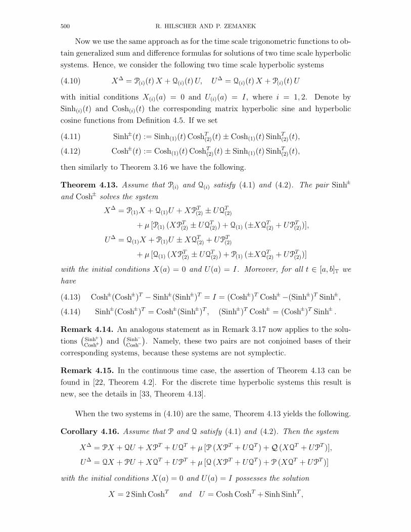
Now we use the same approach as for the time scale trigonometric functions to ob-
tain generalized sum and difference formulas for solutions of two time scale hyperbolic
systems. Hence, we consider the following two time scale hyperbolic systems
(4.10) X∆ = P(i)(t) X + Q(i)(t) U, U∆ = Q(i)(t) X + P(i)(t) U
with initial conditions X(i)(a) = 0 and U(i)(a) = I, where i = 1, 2. Denote by
Sinh(i)(t) and Cosh(i)(t) the corresponding matrix hyperbolic sine and hyperbolic
cosine functions from Definition 4.5. If we set
Sinh±(t) := Sinh(1)(t) CoshT(2)(t) ± Cosh(1)(t) SinhT
(2)(t),(4.11)
Cosh±(t) := Cosh(1)(t) CoshT(2)(t) ± Sinh(1)(t) SinhT
(2)(t),(4.12)
then similarly to Theorem 3.16 we have the following.
Theorem 4.13. Assume that P(i) and Q(i) satisfy (4.1) and (4.2). The pair Sinh±
and Cosh± solves the system
X∆ = P(1)X + Q(1)U + XPT(2) ± UQ
T(2)
+ µ [P(1) (XPT(2) ± UQ
T(2)) + Q(1) (±XQ
T(2) + UP
T(2))],
U∆ = Q(1)X + P(1)U ± XQT(2) + UP
T(2)
+ µ [Q(1) (XPT(2) ± UQ
T(2)) + P(1) (±XQ
T(2) + UP
T(2))]
with the initial conditions X(a) = 0 and U(a) = I. Moreover, for all t ∈ [a, b]T we
have
Cosh±(Cosh±)T − Sinh±(Sinh±)T = I = (Cosh±)T Cosh±−(Sinh±)T Sinh±,(4.13)
Sinh±(Cosh±)T = Cosh±(Sinh±)T , (Sinh±)T Cosh± = (Cosh±)T Sinh± .(4.14)
Remark 4.14. An analogous statement as in Remark 3.17 now applies to the solu-
tions(
Sinh+
Cosh+
)and
(Sinh−
Cosh−
). Namely, these two pairs are not conjoined bases of their
corresponding systems, because these systems are not symplectic.
Remark 4.15. In the continuous time case, the assertion of Theorem 4.13 can be
found in [22, Theorem 4.2]. For the discrete time hyperbolic systems this result is
new, see the details in [33, Theorem 4.13].
When the two systems in (4.10) are the same, Theorem 4.13 yields the following.
Corollary 4.16. Assume that P and Q satisfy (4.1) and (4.2). Then the system
X∆ = PX + QU + XPT + UQ
T + µ [P (XPT + UQ
T ) + Q (XQT + UP
T )],
U∆ = QX + PU + XQT + UP
T + µ [Q (XPT + UQ
T ) + P (XQT + UP
T )]
with the initial conditions X(a) = 0 and U(a) = I possesses the solution
X = 2 Sinh CoshT and U = Cosh CoshT + Sinh SinhT ,
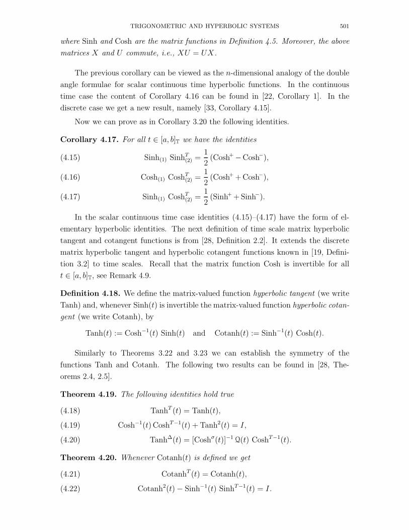
TRIGONOMETRIC AND HYPERBOLIC SYSTEMS 501
where Sinh and Cosh are the matrix functions in Definition 4.5. Moreover, the above
matrices X and U commute, i.e., XU = UX.
The previous corollary can be viewed as the n-dimensional analogy of the double
angle formulae for scalar continuous time hyperbolic functions. In the continuous
time case the content of Corollary 4.16 can be found in [22, Corollary 1]. In the
discrete case we get a new result, namely [33, Corollary 4.15].
Now we can prove as in Corollary 3.20 the following identities.
Corollary 4.17. For all t ∈ [a, b]T we have the identities
Sinh(1) SinhT(2) =
1
2(Cosh+ −Cosh−),(4.15)
Cosh(1) CoshT(2) =
1
2(Cosh+ + Cosh−),(4.16)
Sinh(1) CoshT(2) =
1
2(Sinh+ + Sinh−).(4.17)
In the scalar continuous time case identities (4.15)–(4.17) have the form of el-
ementary hyperbolic identities. The next definition of time scale matrix hyperbolic
tangent and cotangent functions is from [28, Definition 2.2]. It extends the discrete
matrix hyperbolic tangent and hyperbolic cotangent functions known in [19, Defini-
tion 3.2] to time scales. Recall that the matrix function Cosh is invertible for all
t ∈ [a, b]T, see Remark 4.9.
Definition 4.18. We define the matrix-valued function hyperbolic tangent (we write
Tanh) and, whenever Sinh(t) is invertible the matrix-valued function hyperbolic cotan-
gent (we write Cotanh), by
Tanh(t) := Cosh−1(t) Sinh(t) and Cotanh(t) := Sinh−1(t) Cosh(t).
Similarly to Theorems 3.22 and 3.23 we can establish the symmetry of the
functions Tanh and Cotanh. The following two results can be found in [28, The-
orems 2.4, 2.5].
Theorem 4.19. The following identities hold true
TanhT (t) = Tanh(t),(4.18)
Cosh−1(t) CoshT−1(t) + Tanh2(t) = I,(4.19)
Tanh∆(t) = [Coshσ(t)]−1Q(t) CoshT−1(t).(4.20)
Theorem 4.20. Whenever Cotanh(t) is defined we get
CotanhT (t) = Cotanh(t),(4.21)
Cotanh2(t) − Sinh−1(t) SinhT−1(t) = I.(4.22)

502 R. HILSCHER AND P. ZEMANEK
Moreover, if Sinh(t) and Sinhσ(t) are invertible, then
(4.23) Cotanh∆(t) = −[Sinhσ(t)]−1Q(t) SinhT−1(t).
Remark 4.21. In the scalar case n = 1 identities (4.18) and (4.21) are trivial. In the
scalar continuous time case identities (4.19), (4.22), (4.20), and (4.23) take the form
1
cosh2(s)+ tanh2(s) = 1, cotanh2(s) −
1
sinh2(s)= 1, with s =
∫ t
a
Q(τ) dτ ,
(tanh
∫ t
a
Q(τ) dτ
)′
=Q(t)
cosh2 s,
(cotanh
∫ t
a
Q(τ) dτ
)′
=−Q(t)
sinh2 s,
compare with Remark 4.6 (iii). The discrete versions of these identities can be found
in [19, Theorem 3.4] or [32, Theorem 89].
Next, similarly to the definitions of the time scale matrix functions Sinh(i),
Cosh(i), Sinh±, and Cosh± from (4.10)–(4.12) we define
Tanh(i)(t) := Cosh−1(i) (t) Sinh(i)(t), Cotanh(i)(t) := Sinh−1
(i) (t) Cosh(i)(t),
Tanh±(t) := [Cosh±(t)]−1 Sinh±(t), Cotanh±(t) := [Sinh±(t)]−1 Cosh±(t).
Remark 4.22. As in Remark 3.26 we conclude that the first identities from (4.14)
imply the symmetry of the functions Tanh±. Similarly, the functions Cotanh± are
also symmetric.
As it was the case for the trigonometric functions in Theorem 3.27, the results
of the following theorem are new even in the special case of continuous and discrete
time, see also [33, Theorem 4.25].
Theorem 4.23. For all t ∈ [a, b]T such that all involved functions are defined we
have (suppressing the argument t)
Tanh(1) ±Tanh(2) = Tanh(1) (Cotanh(2) ±Cotanh(1)) Tanh(2),(4.24)
Tanh(1) ±Tanh(2) = Cosh−1(1) Sinh± CoshT−1
(2) ,(4.25)
Cotanh(1) ±Cotanh(2) = Cotanh(1) (Tanh(2) ±Tanh(1)) Cotanh(2),(4.26)
Cotanh(1) ±Cotanh(2) = ± Sinh−1(1) Sinh± SinhT−1
(2) ,(4.27)
Tanh± = CoshT−1(2) (I ± Tanh(1) Tanh(2))
−1 (Tanh(1) ±Tanh(2)) CoshT(2),(4.28)
Cotanh± = SinhT−1(2) (Cotanh(2) ±Cotanh(1))
−1 ×(4.29)
× (Cotanh(1) Cotanh(2) ±I) SinhT(2) .
Consider now the system (THS) in the scalar continuous time case with P(t) ≡ 0
and Q(t) ≡ 1, or equivalently system (CHS) with Q(t) ≡ 1. Then the identities
(4.24)–(4.29) have the form of elementary hyperbolic identities.

TRIGONOMETRIC AND HYPERBOLIC SYSTEMS 503
5. CONCLUDING REMARKS
In this paper we extended to the time scale matrix case several identities known
in particular for the scalar continuous time trigonometric and hyperbolic functions.
Namely, for trigonometric functions these are the identity cos2(t) + sin2(t) = 1 in
Corollary 3.10, and the identities displayed in Theorems 3.13, 3.22, and 3.27, Re-
marks 3.15 and 3.24, and Corollaries 3.19 and 3.20. For hyperbolic functions these
are the identity cosh2(t) − sinh2(t) = 1 in Corollary 4.8, and the identities displayed
in Theorems 4.10 and 4.23, Remarks 4.12 and 4.21, and Corollary 4.17.
On the other hand, there are still several trigonometric and hyperbolic identities
which we could not extend to the general time scale matrix case. For example, these
are the identities sin x ± sin y = 2 sin x±y
2cos x∓y
2, as well as other corresponding
identities for the sum or difference of scalar trigonometric and hyperbolic functions.
When y = 0 in the above identity, we get sin x = 2 sin x2
cos x2. The right-hand side is
similar to the solution X(t) in Corollary 3.19, but the left-hand side is not the matrix
function Sin, because the corresponding system is not a trigonometric system (TTS),
see Remark 3.17.
Furthermore, as for the time scale versions of the identities
(5.1)
sin (x + y) sin (x − y) = sin2 x − sin2 y,
cos (x + y) cos (x − y) = cos2 x − sin2 y,
sinh (x + y) sinh (x − y) = sinh2 x − sinh2 y,
cosh (x + y) cosh (x − y) = sinh2 x + cosh2 y,
in the scalar case on an arbitrary time scale we can calculate the products
(5.2)
{Sin+ Sin− = Sin2
(1) − Sin2(2), Sinh+ Sinh− = Sinh2
(1) − Sinh2(2),
Cos+ Cos− = Cos2(1) − Sin2
(2), Cosh+ Cosh− = Sinh2(1) + Cosh2
(2),
because the cross terms cancel due to the commutativity. However, in the general
case the matrix products Sin+ Sin−, Cos+ Cos−, Sinh+ Sinh−, and Cosh+ Cosh− corre-
sponding to the left-hand side of (5.1) do not simplify as in (5.2), since the matrix
multiplication is not commutative.
ACKNOWLEDGEMENT
This research was supported by the Grant Agency of the Academy of Sciences of
the Czech Republic under grant KJB100190701, by the Czech Grant Agency under
grant 201/07/0145, and by the research project MSM 0021622409 of the Ministry of
Education, Youth, and Sports of the Czech Republic. The second author is grateful
to the hospitality of the University of Ulm provided while preparing the final version
of this work.

504 R. HILSCHER AND P. ZEMANEK
The authors wish to thank anonymous referees for their comments which helped
considerably to improve the presentation of this paper.
REFERENCES
[1] C. D. Ahlbrandt, A. C. Peterson, Discrete Hamiltonian Systems: Difference Equations, Con-
tinued Fractions, and Riccati Equations, Kluwer Academic Publishers Group, Dordrecht, 1996.
[2] D. R Anderson, Discrete trigonometric matrix functions, Panamer. Math. J. 7 (1997), no. 1,
39–54.
[3] J.H. Barrett, A Prufer transformation for matrix differential systems, Proc. Amer. Math. Soc.
8 (1957), 510–518.
[4] D. S. Bernstein, Matrix Mathematics. Theory, Facts, and Formulas with Application to Linear
Systems Theory, Princeton University Press, Princeton, 2005.
[5] P. Bohl, Uber eine Differentialgleichung der Storungstheorie, J. Reine Angew. Math. 131 (1906),
268–321.
[6] M. Bohner, O. Dosly, Trigonometric transformations of symplectic difference systems, J. Dif-
ferential Equations 163 (2000), no. 1, 113–129.
[7] M. Bohner, O. Dosly, The discrete Prufer transformations, Proc. Amer. Math. Soc. 129 (2001),
no. 9, 2715–2726.
[8] M. Bohner, O. Dosly, Trigonometric systems in oscillation theory of difference equations, in:
“Dynamic Systems and Applications”, Proceedings of the Third International Conference on
Dynamic Systems and Applications (Atlanta, GA, 1999), Vol. 3, pp. 99–104, Dynamic, Atlanta,
GA, 2001.
[9] M. Bohner, A. Peterson, Dynamic Equations on Time Scales: An Introduction with Applica-
tions, Birkhauser, Boston, 2001.
[10] M. Bohner, A. Peterson, editors, Advances in Dynamic Equations on Time Scales: An Intro-
duction with Applications, Birkhauser, Boston, 2003.
[11] Z. Dosla, D. Skrabakova, Phases of second order linear difference equations and symplectic
systems, Math. Bohem. 128 (2003), no. 3, 293–308.
[12] O. Dosly, On transformations of self-adjoint linear differential systems, Arch. Math. (Brno) 21
(1985), no. 3, 159–170.
[13] O. Dosly, Phase matrix of linear differential systems, Casopis pro pestovanı matematiky 110
(1985), 183–192.
[14] O. Dosly, On some properties of trigonometric matrices, Casopis pro pestovanı matematiky 112
(1987), no. 2, 188–196.
[15] O. Dosly, Riccati matrix differential equation and classification of disconjugate differential sys-
tems, Arch. Math. (Brno) 23 (1987), no. 4, 231–241.
[16] O. Dosly, The Bohl Transformation and its applications, in: “2004–Dynamical Systems and
Applications”, Proceedings of the International Conference (Antalya, 2004), pp. 371–385, GBS
Publishers & Distributors, Delhi, 2005.
[17] O. Dosly, S. Hilger, R. Hilscher, Symplectic dynamic systems, in: “Advances in Dynamic
Equations on Time Scales”, M. Bohner and A. Peterson, editors, pp. 293–334, Birkhauser,
Boston, 2003.
[18] O. Dosly, S. Pechancova, Trigonometric recurrence relations and tridiagonal trigonometric ma-
trices, Internat. J. Difference Equ. 1 (2006), no. 1, 19–29.
TRIGONOMETRIC AND HYPERBOLIC SYSTEMS 505
[19] O. Dosly, Z. Pospısil, Hyperbolic transformation and hyperbolic difference systems, Fasc. Math.
32 (2001), 25–48.
[20] G. J. Etgen, A note on trigonometric matrices, Proc. Amer. Math. Soc. 17 (1966), 1226–1232.
[21] G. J. Etgen, Oscillatory properties of certain nonlinear matrix differential systems of second
order, Trans. Amer. Math. Soc. 122 (1966), 289–310.
[22] K. Filakovsky, Properties of Solutions of Hyperbolic System (in Czech), MSc thesis, University
of J. E. Purkyn, Brno, 1987.
[23] S. Hilger, Analysis on measure chains – A unified approach to continuous and discrete calculus,
Results Math. 18 (1990), no. 1-2, 18–56.
[24] S. Hilger, Matrix Lie theory and measure chains, in: “Dynamic Equations on Time Scales”,
R. P. Agarwal, M. Bohner, and D. O’Regan, editors, J. Comput. Appl. Math. 141 (2002),
no. 1–2, 197–217.
[25] R. Hilscher, V. Zeidan, Time scale symplectic systems without normality, J. Differential Equa-
tions 230 (2006), no. 1, 140–173.
[26] W. Kratz, Quadratic Functionals in Variational Analysis and Control Theory, Akademie Verlag,
Berlin, 1995.
[27] Z. Pospısil, Hyperbolic sine and cosine functions on measure chains, in: “Proceedings of the
Third World Congress of Nonlinear Analysts, Part 2” (Catania, 2000), Nonlinear Anal. 47
(2001), no. 2, 861–872.
[28] Z. Pospısil, Hyperbolic matrix systems, functions and transformations on time scales, author
preprint, October 2001.
[29] Z. Pospısil, An inverse problem for matrix trigonometric and hyperbolic functions on measure
chains, in: “Colloquium on Differential and Difference Equations, CDDE 2002” (Brno), pp. 205–
211, Folia Fac. Sci. Natur. Univ. Masaryk. Brun. Math., Vol. 13, Masaryk Univ., Brno, 2003.
[30] W. T. Reid, A Prufer transformation for differential systems, Pacific J. Math. 8 (1958), 575–584.
[31] W. T. Reid, Ordinary Differential Equations, John Willey & Sons, New York, 1971.
[32] P. Zemanek, Discrete Symplectic Systems (in Czech), MSc thesis, Masaryk University, Brno,
2007.
[33] P. Zemanek, Discrete trigonometric and hyperbolic systems: An overview, in: “Ulmer Sem-
inare”, University of Ulm, Ulm, submitted.
Recommended

![Inverse Trigonometric, COPY Hyperbolic, and Inverse Hyperbolic … · 2015. 3. 4. · [ π/2,π/2]. The new sine function (the solid portion of the graph) does have an inverse, namely](https://img.pdfslide.us/doc/110x75/611baa88dd77c8085b5e20d6/inverse-trigonometric-copy-hyperbolic-and-inverse-hyperbolic-2015-3-4-22.jpg)