Embed Size (px)
Citation preview
QUASI-HYPERBOLIC PLANES IN RELATIVELYHYPERBOLIC GROUPS
JOHN M. MACKAY AND ALESSANDRO SISTO
Abstract. We show that any group that is hyperbolic relativeto virtually nilpotent subgroups, and does not admit peripheralsplittings, contains a quasi-isometrically embedded copy of the hy-perbolic plane. In natural situations, the specific embeddings wefind remain quasi-isometric embeddings when composed with theinclusion map from the Cayley graph to the coned-off graph, aswell as when composed with the quotient map to “almost every”peripheral (Dehn) filling.
We apply our theorem to study the same question for funda-mental groups of 3-manifolds.
The key idea is to study quantitative geometric properties of theboundaries of relatively hyperbolic groups, such as linear connect-edness. In particular, we prove a new existence result for quasi-arcsthat avoid obstacles.
Contents
1. Introduction 21.1. Outline 51.2. Notation 51.3. Acknowledgements 52. Relatively hyperbolic groups and transversality 52.1. Basic definitions 62.2. Transversality and coned-off graphs 82.3. Stability under peripheral fillings 103. Separation of parabolic points and horoballs 123.1. Separation estimates 123.2. Embedded planes 143.3. The Bowditch space is visual 164. Boundaries of relatively hyperbolic groups 174.1. Doubling 184.2. Partial self-similarity 195. Linear Connectedness 21
Date: September 12, 2018.2000 Mathematics Subject Classification. 20F65, 20F67, 51F99.Key words and phrases. Relatively hyperbolic group, quasi-isometric embedding,
hyperbolic plane, quasi-arcs.The research of the first author was supported in part by EPSRC grants
EP/K032208/1 and EP/P010245/1.1
2 JOHN M. MACKAY AND ALESSANDRO SISTO
6. Avoidable sets in the boundary 286.1. Avoiding parabolic points 296.2. Avoiding hyperbolic subgroups 327. Quasi-arcs that avoid obstacles 347.1. Collections of obstacles 357.2. Building the quasi-arc 368. Building quasi-hyperbolic planes 399. Application to 3-manifolds 40References 42
1. Introduction
A well known question of Gromov asks whether every (Gromov)hyperbolic group which is not virtually free contains a surface group.While this question is still open, its geometric analogue has a completesolution. Bonk and Kleiner [BK05], answering a question of Papasoglu,showed the following.
Theorem 1.1 (Bonk–Kleiner [BK05]). A hyperbolic group G containsa quasi-isometrically embedded copy of H2 if and only if it is not vir-tually free.
In this paper, we study when a relatively hyperbolic group admitsa quasi-isometrically embedded copy of H2 by analysing the geometricproperties of boundaries of such groups.
For a hyperbolic group G, quasi-isometrically embedded copies of H2
in G correspond to quasisymmetrically embedded copies of the circleS1 = ∂∞H2 in the boundary of the group. Bonk and Kleiner build sucha circle when a hyperbolic group has connected boundary by observingthat the boundary is doubling (there exists N so that any ball can becovered by N balls of half the radius) and linearly connected (thereexists L so that any points x and y can be joined by a continuum ofdiameter at most Ld(x, y)). For such spaces, a theorem of Tukia appliesto find quasisymmetrically embedded arcs, or quasi-arcs [Tuk96].
We note that this proof relies on the local connectedness of bound-aries of one-ended hyperbolic groups, a deep result following from workof Bestvina and Mess, and Bowditch and Swarup [BM91, Proposition3.3], [Bow98, Theorem 9.3], [Bow99b, Corollary 0.3], [Swa96].
Our strategy is similar to that of Bonk and Kleiner, but to implementthis we have to prove several basic results regarding the geometry ofthe boundary of a relatively hyperbolic group, which we believe are ofindependent interest.
The model for the boundary that we use is due to Bowditch, whobuilds a model space X(G,P) by gluing horoballs into a Cayley graphfor G, and setting ∂∞(G,P) = ∂∞X(G,P) [Bow12] (see also [GM08]).
QUASI-HYPERBOLIC PLANES IN RELATIVELY HYPERBOLIC GROUPS 3
We fix a choice of X(G,P) and, for suitable conditions on the pe-ripheral subgroups, we show that the boundary ∂∞(G,P) has goodgeometric properties. For example, using work of Dahmani and Ya-man, such boundaries will be doubling if and only if the peripheralsubgroups are virtually nilpotent. We establish linear connectednesswhen the peripheral subgroups are one-ended and there are no periph-eral splittings. (See Sections 4 and 5 for precise statements.)
At this point, by Tukia’s theorem, we can find quasi-isometricallyembedded copies of H2 in X(G,P), but these can stray far away fromG into horoballs in X(G,P). To find copies of H2 actually in G itselfwe must prevent this by building a quasi-arc in the boundary that ina suitable sense stays relatively far away from the parabolic points.
This requires additional geometric properties of the boundary (seeSection 6), and also a generalisation of Tukia’s theorem which buildsquasi-arcs that avoid certain kinds of obstacles (Theorem 7.2).
A simplified version of our main result is the following:
Theorem 1.2. Let (G,P) be a finitely generated relatively hyperbolicgroup, where all P ∈ P are virtually nilpotent. Suppose G is one-endedand does not split over a subgroup of a conjugate of some P ∈ P.
Then there is a quasi-isometric embedding of H2 in G.
The methods we develop are able to find embeddings that avoidmore subgroups than just virtually nilpotent peripheral groups. Hereis a more precise version of the theorem:
Theorem 1.3. Suppose both (G,P1) and (G,P1 ∪P2) are finitely gen-erated relatively hyperbolic groups, where all peripheral subgroups in P1
are virtually nilpotent and non-elementary, and all peripheral subgroupsin P2 are hyperbolic. Suppose G is one-ended and does not split over asubgroup of a conjugate of some P ∈ P1.
Finally, suppose that ∂∞H ⊂ ∂∞(G,P1) does not locally disconnectthe boundary, for any H ∈ P2 (see Definition 4.2). Then there is aquasi-isometric embedding of H2 in G that is transversal in (G,P1∪P2).
(Theorem 1.2 follows from Theorem 1.3 by letting P2 = ∅ and P1
equal to the collection of non-elementary elements of P .)Roughly speaking, a quasi-isometric embedding is transversal if the
image has only bounded intersection with any (neighbourhood of a)left coset of a peripheral subgroup (see Definition 2.8). If both P1 andP2 are empty the group is hyperbolic and the result is a corollary ofTheorem 1.1. If P1 is empty, but P2 is not, then the group is hyper-bolic, but the quasi-isometric embeddings we find avoid the hyperbolicsubgroups conjugate to those in P2.
Example 1.4. Let M be a compact hyperbolic 3-manifold with a single,totally geodesic surface as boundary ∂M . The fundamental group G =
4 JOHN M. MACKAY AND ALESSANDRO SISTO
π1(M) is hyperbolic, and also is hyperbolic relative to H = π1(∂M)(see, for example, [Bel07, Proposition 13.1]).
The hypotheses of Theorem 1.3 are satisfied for P1 = ∅ and P2 ={H}, since ∂∞G = ∂∞(G, ∅) is a Sierpinski carpet, with the boundaryof conjugates of H corresponding to the peripheral circles of the carpet.Thus, we find a transversal quasi-isometric embedding of H2 into G.
The notion of transversality is interesting for us, because a transversequasi-isometric embedding of a geodesic metric space Z → G induces:
(1) a quasi-isometric embedding Z → G→ Γ into the coned-off (or
“electrified”) graph Γ (see Proposition 2.11), and(2) a quasi-isometric embedding Z → G → G/ � {Ni} � into
certain peripheral (or Dehn) fillings of G (see Proposition 2.12).
When combined, Theorem 1.3 and Proposition 2.12 provide inter-esting examples of relatively hyperbolic groups containing quasi-iso-metrically embedded copies of H2 that do not have virtually nilpotentperipheral subgroups. A key point here is that Theorem 1.3 providesembeddings transversal to hyperbolic subgroups, and so one can findmany interesting peripheral fillings. See Example 2.14 for details.
Using our results, we describe when the fundamental group of aclosed, oriented 3-manifold contains a quasi-isometrically embeddedcopy of H2. Determining which 3-manifolds (virtually) contain im-mersed or embedded π1-injective surfaces is a very difficult problem[KM12, CLR97, Lac10, BS04, CF17]. The following theorem essen-tially follows from known results, in particular work of Masters andZhang [MZ08, MZ11]. However, our proof is a simple consequence ofTheorem 1.3 and the geometrisation theorem.
Theorem 9.2. Let M be a closed 3-manifold. Then π1(M) contains aquasi-isometrically embedded copy of H2 if and only if M does not splitas the connected sum of manifolds each with geometry S3,R3, S2 × Ror Nil.
Notice that the geometries mentioned above are exactly those thatgive virtually nilpotent fundamental groups.
We note that recently Leininger and Schleimer proved a result simi-lar to Theorem 1.3 for Teichmuller spaces [LS14], using very differenttechniques.
In an earlier version of this paper we claimed a characterisation ofwhich groups hyperbolic relative to virtually nilpotent subgroups ad-mitted a quasi-isometrically embedded copy of H2. This claim wasincorrect due to problems with amalgamations over elementary sub-groups. One cause of trouble is the following:
Example 1.5. Let F2 = 〈a, b〉 be the free group on two generators, andlet H be the Heisenberg group, with centre Z(H) ∼= Z. Let G = F2∗ZH,where we amalgamate the distorted subgroup Z(H) and 〈[a, b]〉 ≤ F2.
QUASI-HYPERBOLIC PLANES IN RELATIVELY HYPERBOLIC GROUPS 5
The group G is hyperbolic relative to {H}, is one-ended, but does notcontain any quasi-isometrically embedded copy of H2.
It remains an open question to characterise which relatively hyper-bolic groups with virtually nilpotent peripheral groups admit quasi-isometrically embedded copies of H2.
Finally, we note that the geometric properties of boundaries of rel-atively hyperbolic groups we establish here have recently been usedby Groves–Manning–Sisto to study the relative Cannon conjecture forrelatively hyperbolic groups [GMS16].
1.1. Outline. In Section 2 we define relatively hyperbolic groups andtheir boundaries, and discuss transversality and its consequences. InSection 3 we give preliminary results linking the geometry of the bound-ary of a relatively hyperbolic group to that of its model space. Furtherresults on the boundary itself are found in Sections 4–6, in particular,how sets can be connected, and avoided, in a controlled manner.
The existence of quasi-arcs that avoid obstacles is proved in Section 7.The proof of Theorem 1.3 is given in Section 8. Finally, connectionswith 3-manifold groups are explored in Section 9.
1.2. Notation. The notation x &C y (occasionally abbreviated to x &y) signifies x ≥ y−C. Similarly, x .C y signifies x ≤ y+C. If x .C yand x &C y we write x ≈C y.
Throughout, C, C1, C2, etc., will refer to appropriately chosen con-stants. The notation C3 = C3(C1, C2) indicates that C3 depends onthe choices of C1 and C2.
For a metric space (Z, d), the open ball with centre z ∈ Z and radiusr > 0 is denoted by B(z, r). The closed ball with the same centre andradius is denoted by B(z, r). We write d(z, V ) for the infimal distancebetween a subset V ⊂ Z and a point z ∈ Z. The open neighbourhoodof V ⊂ Z of radius r > 0 is the set
N(V, r) = {z ∈ Z : d(z, V ) < r}.
1.3. Acknowledgements. We thank Francois Dahmani, Bruce Klein-er, Marc Lackenby, Xiangdong Xie and a referee for helpful comments.
2. Relatively hyperbolic groups and transversality
In this section we define relatively hyperbolic groups and their (Bow-ditch) boundaries. We introduce the notion of a transversal embedding,and show that such embeddings persist into the coned-off graph of arelatively hyperbolic group, or into suitable peripheral fillings of thesame.
6 JOHN M. MACKAY AND ALESSANDRO SISTO
2.1. Basic definitions. There are many (equivalent) definitions of rel-atively hyperbolic groups. We give one here in terms of actions on acusped space. First we define our model of a horoball.
Definition 2.1. Suppose Γ is a connected graph with vertex set Vand edge set E, where every edge has length one. Let T be the strip[0, 1]× [1,∞) in the upper half-plane model of H2. Glue a copy of T toeach edge in E along [0, 1]×{1}, and identify the rays {v}× [1,∞) forevery v ∈ V . The resulting space with its path metric is the horoballB(Γ).
These horoballs are hyperbolic with boundary a single point. (Seethe discussion following [Bow12, Theorem 3.8].) Moreover, it is easyto estimate distances in horoballs.
Lemma 2.2. Suppose Γ and B(Γ) are defined as above. Let dΓ and dBdenote the corresponding path metrics. Then for any distinct verticesx, y ∈ Γ, identified with (x, 1), (y, 1) ∈ B(Γ), we have
dB(x, y) ≈1 2 log(dΓ(x, y)).
Proof. Any geodesic in B(Γ) will project to the image of a geodesic inΓ, so it suffices to check the bound in the hyperbolic plane, for points(0, 1) and (t, 1), with t ≥ 1. But then dB((0, 1), (t, 1)) = arccosh(1+ t2
2),
and ∣∣∣∣arccosh
(1 +
t2
2
)− 2 log(t)
∣∣∣∣is bounded (by 1) for t ≥ 1. �
Definition 2.3. Suppose G is a finitely generated group, and P ={P1, P2, . . . , Pn} a collection of finitely generated subgroups of G. LetS be a finite generating set for G, so that S ∩ Pi generates Pi for eachi = 1, . . . , n.
Let Γ(G) = Γ(G,S) be the Cayley graph of G with respect to S, withword metric dG. Let Y be the disjoint union of Γ(G,S) and copiesBhPi
of B(Γ(Pi, S ∩ Pi)) for each left coset hPi of each Pi. Let X =X(G,P) = Y/ ∼, where for each left coset hPi and each g ∈ hPi theequivalence relation ∼ identifies g ∈ Γ(G,S) with (g, 1) ∈ BhPi
. Weendow X with the induced path metric d, which makes (X, d) a proper,geodesic metric space.
We say that (G,P) is relatively hyperbolic if (X, d) is Gromov hy-perbolic, and call the members of P peripheral subgroups.
This is equivalent to the other usual definitions of (strong) relativehyperbolicity; see [Bow12], [GM08, Theorem 3.25] or [Hru10, Theorem5.1]. (Note that the horoballs of Bowditch and of Groves-Manning arequasi-isometric.)
Let O be the collection of all disjoint (open) horoballs in X, that is,the collection of all connected components of X \Γ(G,S). Note that G
QUASI-HYPERBOLIC PLANES IN RELATIVELY HYPERBOLIC GROUPS 7
acts properly and isometrically on X, cocompactly on X \(⋃
O∈O O),
and the stabilizers of the sets O ∈ O are precisely the conjugates of theperipheral subgroups. Subgroups of conjugates of peripheral subgroupsare called parabolic subgroups.
The boundary of (G,P) is the set ∂∞(G,P) = ∂∞X(G,P) = ∂∞X.Choose a basepoint w ∈ X, and denote the Gromov product in X by(·|·) = (·|·)w; as X is proper, this can be defined as (a|b) = inf{d(w, γ)},where the infimum is taken over all (bi-infinite) geodesic lines γ froma to b; such a geodesic is denoted by (a, b).
A visual metric ρ on ∂∞X with parameters C0, ε > 0 is a metric sothat for all a, b ∈ ∂∞X we have e−ε(a|b)/C0 ≤ ρ(a, b) ≤ C0e
−ε(a|b). AsX is proper and geodesic, for every ε > 0 small enough there exists C0
and a visual metric with parameters C0, ε, see e.g. [GdlH90, Proposition7.10]. We fix such choices of ρ, ε and C0 for the rest of the paper.
For each O ∈ O the set ∂∞O consists of a single point aO ∈ ∂∞Xcalled a parabolic point. We also set dO = d(w,O).
Horoballs can also be viewed as sub-level sets of Busemann functions.
Definition 2.4. Given a point c ∈ ∂∞X, and basepoint w ∈ X, TheBusemann function corresponding to c and w is the function βc(·, w) :X → R defined by
βc(x,w) = supγ
{lim supt→∞
(d(γ(t), x)− t)},
where the supremum is taken over all geodesic rays γ : [0,∞) → Xfrom w to c.
The supremum in this definition is only needed to remove the de-pendence on the choice of γ, however for any two rays from w to c thedifference between the corresponding lim sup values is bounded as afunction of the hyperbolicity constant only, see e.g. [GdlH90, Lemma8.1].
Lemma 2.5. There exists C = C(ε, C0, X) so that for each O ∈ O wehave
{x ∈ X : βaO(x,w) ≤ −dO−C} ⊆ O ⊆ {x ∈ X : βaO(x,w) ≤ −dO+C}.
Proof. One can argue directly, or note that −βaO(·, w) is a horofunctionaccording to Bowditch’s definition, and so the claim follows from thediscussion before [Bow12, Lemma 5.4]. �
From now on, for any Gromov hyperbolic metric space Y we denoteby δY a hyperbolicity constant of Y , i.e. given any geodesic trianglewith vertices in Y ∪ ∂Y , each side of the triangle is contained in theunion of the δY -neighbourhoods of the other two sides.
Lemma 2.6. Let (G,P) be relatively hyperbolic, and X = X(G,P) asabove. For any left coset gP of some P ∈ P and any x, y ∈ gP , all
8 JOHN M. MACKAY AND ALESSANDRO SISTO
geodesics from x to y are contained in the corresponding O ∈ O exceptfor, at most, an initial and a final segment of length at most 2δX + 1.
Proof. From the definition of a horoball, any “vertical” ray {v}×[1,∞)in O is a geodesic ray in both X and O. Also, for any v ∈ gP andt ≥ 1, the closest point in X \O to (v, t) ∈ O is (v, 1) ∈ O.
Consider a geodesic triangle with sides {x} × [1,∞), {y} × [1,∞)and a geodesic γ in X from x to y. If p ∈ γ has distance greater than2δX + 1 from both x and y, then it is δX close to a point q on one ofthe vertical rays, which has distance at least δX + 1 from {x, y}. Asd(q,X \O) = d(q, {x, y}), we have d(p,X \O) ≥ 1 and p ∈ O. �
Finally, we extend the distance estimate of Lemma 2.2 to X.
Lemma 2.7. Let (G,P) be relatively hyperbolic, and X = X(G,P) asabove. There exists A = A(X) < ∞ so that for any left coset gP ofsome P ∈ P, with metric dP , for any distinct x, y ∈ gP , we have
d(x, y) ≈A 2 log(dP (x, y)).
Proof. Consider a geodesic γ from x to y. If d(x, y) ≤ 4δX + 3, thenthere is a uniform upper bound of C = C(X) on dP (x, y) as dP is aproper function with respect to d, so this case is done. Otherwise, byLemma 2.6, γ has a subgeodesic γ′ connecting points x′, y′ ∈ gP , withγ′ entirely contained in the horoball O that corresponds to gP , andd(x, y) ≈4δX+2 d(x′, y′), so d(x′, y′) ≥ 1. In particular, x′ 6= y′.
As before, dP (x, x′) and dP (y, y′) are both at most C. Let dB denotethe horoball distance for points in O. Notice that d(x′, y′) = dB(x′, y′)as γ′ is a geodesic in X connecting x′ to y′ entirely contained in O.Using Lemma 2.2 we have
d(x, y) ≈4δX+2 d(x′, y′) = dB(x′, y′)
≈1 2 log(dP (x′, y′)) ≈C′ 2 log(dP (x, y)),
for an appropriate constant C ′ = C ′(C). �
2.2. Transversality and coned-off graphs. Our goal here is to de-fine transversality of quasi-isometric embeddings, and show that atransversal quasi-isometric embedding of H2 in Γ = Γ(G) will per-sist if we cone-off the Cayley graph. Recall that a function f : X → X ′
between metric spaces is a (λ,C)-quasi-isometric embedding (for someλ ≥ 1, C ≥ 0) if for all x, y ∈ X,
1
λd(x, y)− C ≤ d(f(x), f(y)) ≤ λd(x, y) + C.
We continue with the notation of Definition 2.3.
Definition 2.8. Let (G,P) be a relatively hyperbolic group. Let Z bea geodesic metric space. Given a function η : [0,∞)→ [0,∞), a quasi-isometric embedding f : Z → (G, dG) is η-transversal if for all M ≥ 0,g ∈ G, and P ∈ P, we have diam(f(Z) ∩N(gP,M)) ≤ η(M).
QUASI-HYPERBOLIC PLANES IN RELATIVELY HYPERBOLIC GROUPS 9
A quasi-isometric embedding f : Z → G is transversal if it is η-transversal for some such η.
Let Γ be the coned-off graph of Γ(G): for every left coset hP of everyP ∈ P , add a vertex to Γ, and add edges of length 1/2 joining this ver-
tex to each g ∈ hP . Let c : Γ→ Γ be the natural inclusion. This graphis hyperbolic, by the equivalent definition of relative hyperbolicity in[Far98] (see also [Hru10, Definition 3.6]). Recall that a λ-quasi-geodesicis a (λ, λ)-quasi-isometric embedding of an interval (which need not becontinuous).
Lemma 2.9. Let (G,P) be a relatively hyperbolic group. If α : R →(G, dG) is an η-transversal λ-quasi-geodesic, then c(α) is a λ′-quasi-
geodesic in Γ, where λ′ = λ′(λ, η,G,P). Moreover, α is also a λ′-quasi-geodesic in X(G,P).
Proof. On Γ we have 1CdΓ ≤ dX ≤ dG for a suitable C ≥ 1, and
α : R → (G, dG) is a (λ, λ)-quasi-isometry. Therefore, it suffices to
show that for some λ′ = λ′(λ, η, Γ), for any x1, x2 ∈ α, we have
(2.10) dΓ(x1, x2) ≥ 1λ′dG(x1, x2)− λ′.
Let γ be the sub-quasi-geodesic of α with endpoints x1, x2. Let γ bea geodesic in Γ with endpoints c(x1), c(x2).
Now let π : Γ→ γ be a closest point projection map, fixing x1, x2. AsΓ is hyperbolic, such a projection map is coarsely Lipschitz : there existsC1 = C1(Γ) so that for all x, y ∈ Γ, dΓ(π(x), π(y)) ≤ C1dΓ(x, y) + C1.
By [Hru10, Lemma 8.8], there exists C2 = C2(G,P , λ) so that every
vertex of γ is at most a distance C2 from γ in Γ (not just Γ). Letπ′ : (γ, dΓ)→ (γ, dG) be a map so that for all x ∈ γ, dG(π′(x), x) ≤ C2,and assume that π′ fixes x1, x2. This map is coarsely Lipschitz also. Itsuffices to check this for vertices x, y ∈ γ ∩ Γ with dΓ(x, y) = 1. If xand y are connected by an edge of Γ, then clearly dG(π′(x), π′(y)) ≤2C2 + 1. Otherwise, π′(x), π′(y) are both in γ and within distanceC2 of the same left coset of a peripheral group, so by transversality,dG(π′(x), π′(y)) ≤ η(C2).
Thus, for C3 = max{2C2 + 1, η(C2)}, (2.10) with λ′ = C3C1 followsfrom
dG(x1, x2) = dG(π′ ◦ π(x1), π′ ◦ π(x2)) ≤ C3dΓ(π(x1), π(x2))
≤ C3(C1dΓ(x1, x2) + C1). �
Proposition 2.11. Suppose Z is a geodesic metric space, and (G,P)a relatively hyperbolic group. If a quasi-isometric embedding f : Z →G is transversal then c ◦ f : Z → Γ is a quasi-isometric embedding,quantitatively.
Proof. By Lemma 2.9, whenever γ is a geodesic in Z, c ◦ f(γ) is a
quasi-geodesic with uniformly bounded constants in Γ. �
10 JOHN M. MACKAY AND ALESSANDRO SISTO
2.3. Stability under peripheral fillings. We now consider periph-eral fillings of (G, {P1, . . . , Pn}). The results here are not used in theremainder of the paper.
Suppose Ni / Pi are normal subgroups. The peripheral filling of Gwith respect to {Ni} is defined as
G({Ni}) = G/�⋃i
Ni � .
(See [Osi07] and [GM08, Section 7].) Let p : G → G({Ni}) be thequotient map.
Proposition 2.12. Let (G,P) be a relatively hyperbolic group, andG({Ni}) a peripheral filling of G, as defined above.
Let Z be a geodesic metric space, and suppose that f : Z → G isan η-transversal (λ, λ)-quasi-isometric embedding. There exists R0 =R0(η, λ,G,P) so that if B(e, R0) ∩ Ni = {e} for each i, then p ◦ f :Z → G({Ni}) is a quasi-isometric embedding.
Proof. We will use results from [DGO17] (see also [DG08, Cou11]).For any sufficiently large R0 we combine Propositions 7.7 and 5.28 in[DGO17] to show that G({Ni}) acts on a certain δ′-hyperbolic space Y(namely Y = X′/Rot for X′ and Rot arising from R in the notation of[DGO17]), with the following properties:
(1) δ′ only depends on the hyperbolicity constant of X = X(G,P),(2) there is a 1-Lipschitz map ψ : G({Ni})→ Y (this follows from
the construction of Y and the fact that the inclusion of G in Xis 1-Lipschitz),
(3) there is a map φ : (N(G,L) ⊆ X) → Y such that, for eachg ∈ G, φ|B(g,L) is an isometry, where L = L(R0, X) → ∞ asR0 →∞.
(4) ψ ◦ p = φ ◦ ι, where ι : G→ X is the natural inclusion.
Let γ be any geodesic in Z. By Lemma 2.9, ι◦f(γ) is a λ′-quasi-geodesicin X, for λ′ = λ′(λ, η,G,P). Let α be a geodesic in X connecting theendpoints of ι ◦ f(γ). Let C1 = C1(δ′, λ′) bound the distance betweeneach point on α and G ⊆ X.
Suppose that L as in (3) satisfies L ≥ C1 + 8δ′ + 1. Then foreach x ∈ α we have that φ|B(x,8δ′+1) is an isometry, and so [BH99,Theorem III.H.1.13-(3)] gives that φ(α) is a C2-quasi-geodesic, whereC2 = C2(δ′). This implies that (φ ◦ ι ◦ f)(γ) is a C3-quasi-geodesic,with C3 = C3(C1, C2). Let x1, x2 be the endpoints of γ. Using (2) and(4) above, we see that
dG({Ni})(p ◦ f(x1), p ◦ f(x2)) ≥ dY (ψ ◦ p ◦ f(x1), ψ ◦ p ◦ f(x2))
= dY (φ ◦ ι ◦ f(x1), φ ◦ ι ◦ f(x2))
≥ 1C3dZ(x1, x2)− C3.
QUASI-HYPERBOLIC PLANES IN RELATIVELY HYPERBOLIC GROUPS 11
On the other hand, recall that p is 1-Lipschitz, so
dG({Ni})(p ◦ f(x1), p ◦ f(x2)) ≤ dG(f(x1), f(x2)) ≤ λdZ(x1, x2) + λ.
As γ was arbitrary, we are done. �
As discussed in the introduction, we can use Proposition 2.12 tofind interesting examples of relatively hyperbolic groups with quasi-isometrically embedded copies of H2, but whose peripheral groups arenot virtually nilpotent. We note the following lemma.
Lemma 2.13. Let F4 be the free group with four generators, and letR be fixed. Then there are normal subgroups {Kα}α∈R of F4 so thatthe quotient groups F4/Kα are amenable but not virtually nilpotent, sothat if α 6= β then F4/Kα and F4/Kβ are not quasi-isometric, and sothat Kα ∩B(e, R) = {e}.
Proof. It is shown in [Gri84] that there is an uncountable family of4-generated groups {F4/K
′α}α∈R of intermediate growth with distinct
growth rates. In particular, these groups are amenable, not virtuallynilpotent and pairwise non-quasi-isometric. To conclude the proof, letK be a finite index normal subgroup of F4 so that K ∩B(e, R) = {e},and let Kα = K ′α ∩K C F4. As F4/Kα is a finite extension of F4/K
′α,
it inherits all the properties above. �
Example 2.14. Let M be a closed hyperbolic 3-manifold so that G =π1(M) is hyperbolic relative to a subgroup P ≤ G that is isomorphicto F4. For example, let M ′ be a compact hyperbolic manifold whoseboundary ∂M ′ is a totally geodesic surface of genus 3, and let M be thedouble of M ′ along ∂M ′. Observe that π1(M) is hyperbolic relative toπ1(∂M ′), and π1(∂M ′) is hyperbolic relative to a copy of π1(S ′) = F4,where S ′ ⊂ ∂M ′ is a punctured genus 2 subsurface. Thus π1(M) ishyperbolic relative to π1(S ′).
Since G is hyperbolic with 2-sphere boundary, and P is quasi-convexin G with Cantor set boundary (Lemma 3.1(2)), the hypotheses of The-orem 1.3 are satisfied for P1 = ∅ and P2 = {P}. Therefore, we find atransversal quasi-isometric embedding of H2 into G.
Let R0 be chosen by Proposition 2.12. As P is quasi-convex in G,we choose R so that for x ∈ P , if dP (e, x) ≥ R then dG(e, x) ≥ R0.Now let {Kα} be the subgroups constructed in Lemma 2.13. By Propo-sition 2.12, for each α ∈ R the peripheral filling Gα = G/� Kα � isrelatively hyperbolic and contains a quasi-isometrically embedded copyof H2.
As P/Kα is non-virtually cyclic and amenable, it does not have anon-trivial relatively hyperbolic structure. Therefore, Gα is not hy-perbolic relative to virtually nilpotent subgroups, for in any peripheralstructure P, some peripheral group H ∈ P must be quasi-isometric toP/Kα by [BDM09, Theorem 4.8].
12 JOHN M. MACKAY AND ALESSANDRO SISTO
Finally, if α 6= β then Gα is not quasi-isometric to Gβ by [BDM09,Theorem 4.8] as P/Kα and P/Kβ are not quasi-isometric.
3. Separation of parabolic points and horoballs
In this section we study how the boundaries of peripheral subgroupsare separated in ∂∞X. We also establish a preliminary result on quasi-isometrically embedding copies of H2.
3.1. Separation estimates. We begin with the following lemma.
Lemma 3.1. Let (G,P1) and (G,P1 ∪ P2) be relatively hyperbolicgroups, where all peripheral subgroups in P2 are hyperbolic groups (P2
is allowed to be empty), and set X = X(G,P1). Let H denote thecollection of the horoballs of X and the left cosets of the subgroups inP2; more precisely, the images of those left cosets under the naturalinclusion G ↪→ X. For H ∈ H, let dH = d(w,H).
Then the collection of subsets H has the following properties.
(1) For each r ≥ 0 there is a uniform bound b(r) on diam(N(H, r)∩N(H ′, r)) for each H,H ′ ∈ H with H 6= H ′.
(2) Each H ∈ H is uniformly quasi-convex in X.(3) There exists R such that, given any H ∈ H and any geodesic
ray γ connecting w to a ∈ ∂∞H, the subray of γ whose startingpoint has distance dH from w is entirely contained in N(H,R).
Proof. In this proof we use results from [DS05], which uses the equiva-lent definition that (G,P) is relatively hyperbolic if and only the Cayleygraph of G is “asymptotically tree graded” with respect to the collec-tion of left cosets of groups in P [DS05, Definition 5.9, Theorem 8.5].
We first show (1). Let gP, g′P ′ be the left cosets correspondingto H,H ′. As G acts properly on X, given r there exists r′ so thatN(H, r) ∩ N(H ′, r) (using the metric d on X) is contained in the r′-neighbourhood in X of NG(gP, r′) ∩NG(g′P ′, r′) ⊂ G ⊂ X (where NG
indicates that we use the metric dG). The diameter of NG(gP, r′) ∩NG(g′P ′, r′) has a uniform bound in G by [DS05, Theorem 4.1(α1)]; asd ≤ dG it is also uniformly bounded in X.
Let us show (2). Uniform quasi-convexity of the horoballs is a conse-quence of Lemma 2.6. If H is a left coset of a peripheral subgroup in P2,then it is quasi-convex in the Cayley graph Γ of G [DS05, Lemma 4.15].What is more, by [DS05, Theorem 4.1(α1)], geodesics in Γ connectingpoints of H are transversal with respect to P1. Therefore, by Lemma2.9 they are quasi-geodesics in X. We conclude that H is quasi-convexin X since pairs of points of H can be joined by quasi-geodesics (withuniformly bounded constants) which stay uniformly close to H.
We now show (3). Choose p ∈ H so that d(w, p) ≤ dH + 1. Asa ∈ ∂∞H and H is quasi-convex, there exists C = C(X) so that ageodesic ray γ′ from p to a lies in the C-neighbourhood of H.
QUASI-HYPERBOLIC PLANES IN RELATIVELY HYPERBOLIC GROUPS 13
Choose x on a geodesic γ′′ from w to p so that d(w, x) = dH − C −δX − 1. We must have d(x, γ′) > δX , otherwise d(w,H) ≤ d(w, x) +d(x, γ′) + C < dH . As the geodesic triangle with sides γ, γ′, γ′′ is δXthin, x is within dX of a point y ∈ γ. Note that d(y,H) ≤ C+ 2δX + 1,so by (2) the subray of γ starting at y lies in a uniformly boundedneighbourhood of H. As d(w, y) ≤ dH −C − 1 < dH , we are done. �
From this lemma, we can deduce separation properties for the bound-aries of sets in H.
Lemma 3.2. We make the assumptions of Lemma 3.1. Then thereexists C = C(X) so that for each H,H ′ ∈ H with H 6= H ′ and dH ≥dH′ we have
ρ(∂∞H, ∂∞H′) ≥ e−εdH/C.
Proof. Let a ∈ ∂∞H, a′ ∈ ∂∞H ′. We have to show that (a|a′) . dH .Let γ, γ′ be rays connecting w to a, a′, respectively. For each p ∈ γ suchthat d(w, p) ≤ (a|a′) there exists p′ ∈ γ′ such that d(p′, w) = d(p, w)and d(p, p′) ≤ C1 = C1(δX). With b(r) and R as found by Lemma 3.1,set C2 = b(R + C1).
Suppose that (a|a′) ≥ dH +C2 + 1. Consider p ∈ γ, p′ ∈ γ such thatd(p, w) = d(p′, w) = dH . By Lemma 3.1(3), we have p ∈ N(H,R) andp′ ∈ N(H ′, R), as dH ≥ dH′ . So, p ∈ N(H,R+C1)∩N(H ′, R+C1). Thesame holds also when p ∈ γ is such that d(p, w) = dH+C2+1. Thereforewe have diam(N(H,R + C1) ∩ N(H ′, R + C1)) > C2, contradictingLemma 3.1(1). Hence (a|a′) < dH + C2 + 1, and we are done. �
Conversely, we show that separation properties of certain points inthe boundary ∂∞X have implications for the intersection of sets in X.
Lemma 3.3. We make the assumptions of Lemma 3.1.Let γ be a geodesic line connecting w to a ∈ ∂∞X. Suppose that
for some H ∈ H and r ≥ 1 we have ρ(a, ∂∞H) ≥ e−εdH/r. Thenγ intersects N(H,L) in a set of diameter bounded by K + 2L, forK = K(r,X) and any L ≥ 0.
Proof of Lemma 3.3. We will treat the horoball case and the left cosetcase separately, beginning with the latter.
We can assume that H is not bounded, for otherwise the lemma istrivially true. Due to quasi-convexity, each point on H is at uniformlybounded distance from a geodesic line connecting points a1, a2 in ∂∞H,and thus also at uniformly bounded distance, say C1 = C1(X), fromeither a ray connecting w to a1 or a ray connecting w to a2.
Let c ∈ ∂∞H and let γ′ be a ray connecting w to c. As ρ(a, c) ≥e−εdH/r, we have that (a|c) ≤ dH + r′ + C2, for r′ = log(r)/ε andC2 = C2(δX , ε, C0).
There exists C3 = C3(C1, X) so that any point x on γ such thatd(x,w) ≥ (a|c) +L+C3 has the property that d(x, γ′) ≥ L+C1. Thisapplies to all rays connecting w to some c ∈ ∂∞H, and so d(x,H) > L.
14 JOHN M. MACKAY AND ALESSANDRO SISTO
Also, if x ∈ γ and d(x,w) < dH − L then clearly d(x,H) > L. Thusif γ ∩N(H,L) 6= ∅ we have (a|c) + L+ C3 ≥ dH − L, and
diam(γ ∩N(H,L)) ≤ (a|c) + L+ C3 − (dH − L) .C2+C3 r′ + 2L.
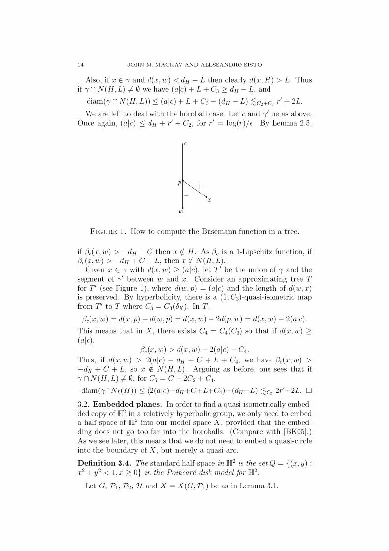
We are left to deal with the horoball case. Let c and γ′ be as above.Once again, (a|c) ≤ dH + r′ + C2, for r′ = log(r)/ε. By Lemma 2.5,
Figure 1. How to compute the Busemann function in a tree.
if βc(x,w) > −dH + C then x /∈ H. As βc is a 1-Lipschitz function, ifβc(x,w) > −dH + C + L, then x /∈ N(H,L).
Given x ∈ γ with d(x,w) ≥ (a|c), let T ′ be the union of γ and thesegment of γ′ between w and x. Consider an approximating tree Tfor T ′ (see Figure 1), where d(w, p) = (a|c) and the length of d(w, x)is preserved. By hyperbolicity, there is a (1, C3)-quasi-isometric mapfrom T ′ to T where C3 = C3(δX). In T ,
βc(x,w) = d(x, p)− d(w, p) = d(x,w)− 2d(p, w) = d(x,w)− 2(a|c).This means that in X, there exists C4 = C4(C3) so that if d(x,w) ≥(a|c),
βc(x,w) > d(x,w)− 2(a|c)− C4.
Thus, if d(x,w) > 2(a|c) − dH + C + L + C4, we have βc(x,w) >−dH + C + L, so x /∈ N(H,L). Arguing as before, one sees that ifγ ∩N(H,L) 6= ∅, for C5 = C + 2C2 + C4,
diam(γ∩NL(H)) ≤ (2(a|c)−dH+C+L+C4)−(dH−L) .C5 2r′+2L. �
3.2. Embedded planes. In order to find a quasi-isometrically embed-ded copy of H2 in a relatively hyperbolic group, we only need to embeda half-space of H2 into our model space X, provided that the embed-ding does not go too far into the horoballs. (Compare with [BK05].)As we see later, this means that we do not need to embed a quasi-circleinto the boundary of X, but merely a quasi-arc.
Definition 3.4. The standard half-space in H2 is the set Q = {(x, y) :x2 + y2 < 1, x ≥ 0} in the Poincare disk model for H2.
Let G, P1, P2, H and X = X(G,P1) be as in Lemma 3.1.
QUASI-HYPERBOLIC PLANES IN RELATIVELY HYPERBOLIC GROUPS 15
Proposition 3.5. Let f : Q → X be a (µ, µ)-quasi-isometric embed-ding of the standard half-space H2 into X, with f((0, 0)) = w. Supposethere exists λ > 0 so that for each a ∈ ∂∞Q, H ∈ H we have
d(f(a), ∂∞H) ≥ e−εdH/λ.
Then there exists a transversal (with respect to P = P1 ∪ P2) quasi-isometric embedding g : H2 → Γ(G).
Proof. Each point x ∈ Q\{(0, 0)} lies on a unique geodesic γx connect-ing (0, 0) to a point ax in ∂∞Q. As f(γx) is a µ-quasi-geodesic and X ishyperbolic, f(γx) lies within distance C1 = C1(µ, δX) from a geodesicγ′x from w to f(ax). Let x′ ∈ γ′x satisfy d(f(x), x′) ≤ C1.
Given two such points x, y ∈ Q \ {(0, 0)}, let x′′, y′′ be the pointson γ′x, γ
′y at distance (x′|y′) from w. By hyperbolicity, d(x′′, y′′) ≤ C,
and and x′′, y′′ both lie within C of any geodesic γx′y′ from x′ to y′, forC = C(δX).
If f(x) and f(y) lie inN(H,L), for someH ∈ H, L ≥ 0, then γx′y′ liesin N(H,L′), for some L′ = L′(L, δX ,H, C1), by the quasiconvexity of H(Lemma 3.1(2)). Thus x′, x′′, y′, y′′ are in N(H,L′+C). By Lemma 3.3,d(x′′, x′) and d(y′′, y′) are both at most C ′ = K + 2(L′ + C), for K =K(λ,X). Thus d(f(x), f(y)) ≈2C1+C d(x′′, x′) + d(y′, y′′) ≤ 2C ′, so wehave the bound
(3.6) diam(N(H,L) ∩ f(Q)) ≤ 2C ′ + 2C1 + C.
In particular, any point on γ′x is C2 = C2(λ,X) close to a point inΓ(G), and therefore any point in f(Q) is C1 + C2 close to a point inΓ(G).
Notice that Q contains balls {Bn} of H2 of arbitrarily large radius,each of which admits a (µ, µ)-quasi-isometric embedding fn : Bn → Xso that each point in fn(Bn) is a distance C1 + C2 close to a pointin Γ(G). In particular, translating those embeddings appropriatelyusing the action of G on X we can and do assume that the centerof Bn is mapped at uniformly bounded distance from w. As X isproper, we can use Arzela-Ascoli to obtain a (µ′, µ′)-quasi-isometricembedding g : H2 → X as the limit of a subsequence of {fn} (moreprecisely {fn|N}, where N is a maximal 1-separated net in H2), forµ′ = µ′(µ,C1, C2).
We now define g : H2 → Γ(G) so that for each x ∈ H2 we haved(g(x), g(x)) ≤ C3, for C3 = C3(C1, C2). As H is invariant under theaction of G, and dG is a proper function of d, g is transversal by (3.6).
It remains to show that g is a quasi-isometric embedding. Pick x, y ∈H2. Notice that
dG(g(x), g(y)) ≥ d(g(x), g(y)) &2C3 d(g(x), g(y)) &µ′ d(x, y)/µ′,
so it suffices to show that for some µ′′,
dG(g(x), g(y)) ≤ µ′′d(g(x), g(y)) + µ′′.
16 JOHN M. MACKAY AND ALESSANDRO SISTO
Let γ be the geodesic in H2 connecting x to y. Let γ′ be the piecewisegeodesic in X from g(x) to g(x) to g(y) to g(y), which is at Hausdorffdistance at most C4 = C4(µ′, C3, δX) from g(γ).
Each maximal subpath β ⊆ γ′ contained in some horoball O ∈ Ohas length l(β) at most C5 = C5(C4, X) by transversality (3.6). Ifz, z′ ∈ G are the endpoints of β, then dG(z, z′) ≤ Md(z, z′), for someM = M(C5, X) ≥ 1, as dG is a proper function of d, and if z 6= z′ thend(z, z′) is uniformly bounded away from zero. So we can substitute βby a subpath in Γ(G) of length at most Ml(β).
Let α be the path in Γ(G) obtained from γ′ by substituting eachsuch β in this way. Clearly we have l(α) ≤Ml(γ′), and so
dG(g(x), g(y)) ≤ l(α) ≤M(d(g(x), g(y)) + 2C3). �
3.3. The Bowditch space is visual. In order for the boundary of aGromov hyperbolic space to control the geometry of the space itself,we require the following standard property.
Definition 3.7. A proper, geodesic, Gromov hyperbolic space X isvisual if there exists w ∈ X and C > 0 so that for every x ∈ X thereexists a geodesic ray γ : [0,∞)→ X, with γ(0) = w and d(x, γ) ≤ C.
A weaker version of this condition, suitable for spaces that are notproper, or not geodesic, is given in [BS00, Section 5].
We record the following observation for completeness.
Proposition 3.8. If (G,P) is a relatively hyperbolic group with everyP ∈ P a proper subgroup of G, then X(G,P) is visual.
Proof. Let w ∈ X = X(G,P) be the point corresponding to e ∈ G.Let x ∈ X be arbitrary.
First we assume that P 6= ∅. The point x lies in N(O, 1), for some(possibly many) O ∈ O. Let aO = ∂∞O be the parabolic point cor-responding to O, and let b ∈ ∂∞X \ {aO} be any other point. Sucha point exists as the peripheral group corresponding to O has infiniteindex in G.
As X is proper and geodesic, there is a bi-infinite geodesic lineγ : (−∞,∞) → X with endpoints aO and b. The parabolic groupcorresponding to O acts on X, stabilising aO ∈ ∂∞X, so that sometranslate γ′ of γ is at distance at most C from the point x. (We cantake C = 2.)
Denote the endpoints of γ′ by aO and b′, and let α be the geodesicray from w to aO, and β the geodesic ray from w to b′. As the geodesictriangle γ′, α, β is δX-thin, x lies within a distance of C + δX of one ofthe geodesic rays α and β, and we are done.
Secondly, if P = ∅, we have that X(G, ∅) is a Cayley graph of G. Fixany a 6= b in ∂∞X. As X is proper and geodesic, there is a bi-infinitegeodesic γ from a to b. As the action of G on X is cocompact, some
QUASI-HYPERBOLIC PLANES IN RELATIVELY HYPERBOLIC GROUPS 17
translate of γ passes within a uniformly bounded distance of x, andthe proof proceeds as in the first case. �
4. Boundaries of relatively hyperbolic groups
We now begin our study of the geometry of the boundary of a rela-tively hyperbolic group, endowed with a visual metric ρ as in Section 2.In this section, we study the properties of being doubling and havingpartial self-similarity.
First, we summarize some known results about the topology of suchboundaries.
Theorem 4.1 (Bowditch). Suppose (G,P) is a one-ended relativelyhyperbolic group which does not split over a subgroup of a conjugate ofsome P ∈ P, and every group in P is finitely presented, one or twoended, and contains no infinite torsion subgroup. Then ∂∞(G,P) isconnected, locally connected and has no global cut points.
Proof. Connectedness and local connectedness follow from [Bow12, Pro-position 10.1] and [Bow99a, Theorem 0.1].
Any global cut point must be a parabolic point [Bow99b, Theorem0.2], but the splitting hypothesis ensures that these are not global cutpoints either [Bow99a, Proposition 5.1, Theorem 1.2]. �
Recall that a point p in a connected, locally connected, metrisabletopological space Z is not a local cut point if for every connected neigh-bourhood U of p, the set U \ {p} is also connected. If, in addition, Zis compact, then Z is locally path connected, so p is not a local cutpoint if and only if every neighbourhood U of p contains an open Vwith p ∈ V ⊂ U and V \ {p} path connected.
More generally, we have the following definition, used in the state-ment of Theorem 1.3.
Definition 4.2. A closed set V ( Z in a connected, locally connected,metrisable topological space Z does not locally disconnect Z if for anyopen connected U ⊂ Z, the set U \ V is also connected.
For relatively hyperbolic groups, we note the following.
Proposition 4.3. Suppose (G,P) is relatively hyperbolic with con-nected and locally connected boundary. Let p be a parabolic point in∂∞(G,P) which is not a global cut-point. Then p is a local cut point ifand only if the corresponding peripheral group has more than one end.
Proof. The lemma follows, similarly to the proof of [Dah05, Proposi-tion 3.3], from the fact that the parabolic subgroup P correspondingto p acts properly discontinuously and cocompactly on ∂∞(G,P)\{p},which is connected and locally connected. Let us make this precise.
Choose an open set K0 with compact closure in ∂∞(G,P)\{p}, sothat PK0 = ∂∞(G,P)\{p}. Then define K1 as the union of all qK0 for
18 JOHN M. MACKAY AND ALESSANDRO SISTO
q ∈ P with dP (q, e) ≤ 1. As ∂∞(G,P)\{p} is connected and locallypath connected, and K1 is compact, one can easily find an open, pathconnected K so that K1 ⊂ K ⊂ K ⊂ ∂∞(G,P)\{p}.
Now suppose that P has one end. Let U be a neighbourhood of p.As P acts properly discontinuously on ∂∞(G,P)\{p}, there exists R sothat if dP (e, g) > R, then gK ⊂ U . Let Q be the unbounded connectedcomponent of P \B(e, R). Then QK is path connected as for g, h ∈ P ,if dP (g, h) ≤ 1, gK∩hK 6= ∅. Finally, observe that V = QK∪{p} ⊂ Uis a neighbourhood of p so that V \ {p} = QK is connected.
Conversely, suppose that p is not a local cut-point. Let D be so thatif qK ∩ rK 6= ∅ then dP (q, r) ≤ D. Suppose we are given R > 0. Wecan find a connected neighbourhood U of p in ∂∞(G,P) so that U \{p}is path connected and gK ∩ U = ∅ for all g ∈ B(e, R + D) ⊂ P . LetR′ ≥ R+D be chosen so that gK∩U 6= ∅ for all g ∈ P \B(e, R′). Giveng, h ∈ P\B(e, R′) we can find a path in U\{p} connecting gK to hK.So, there exists a sequence g = g0, g1, . . . , gn = h in P \B(e, R+D) sothat giK ∩gi+1K 6= ∅ for all i = 0, . . . , n−1. Thus as dP (gi, gi+1) ≤ D,we have that g and h can be connected in P outside B(e, R). As Rwas arbitrary, P is one-ended. �
4.1. Doubling.
Definition 4.4. A metric space (X, d) is N -doubling if every ball canbe covered by at most N balls of half the radius.
Every hyperbolic group has doubling boundary, but this is not thecase for relatively hyperbolic groups.
Proposition 4.5. The boundary of a relatively hyperbolic group (G,P)is doubling if and only if every peripheral subgroup is virtually nilpotent.
Recall that all relatively hyperbolic groups we consider are finitelygenerated, with P a finite collection of finitely generated peripheralgroups.
Proof. By [DY05, Theorem 0.1], every peripheral subgroup is virtuallynilpotent if and only if X = X(G,P) has bounded growth at all scales:for every 0 < r < R there exists some N so that every radius R ball inX can be covered by N balls of radius r.
If X has bounded growth at some scale then ∂∞X is doubling [BS00,Theorem 9.2].
On the other hand, if ∂∞X is doubling, then ∂∞X quasisymmet-rically embeds into some Sn−1 (see [Ass83], or [Hei01, Theorem 12.1]).Therefore, X quasi-isometrically embeds into some Hn [BS00, Theo-rems 7.4, 8.2], which has bounded growth at all scales. We concludethat X has bounded growth at all scales (for small scales, the boundedgrowth of X follows from the finiteness of P , and the finite generationof G and all peripheral groups). �
QUASI-HYPERBOLIC PLANES IN RELATIVELY HYPERBOLIC GROUPS 19
4.2. Partial self-similarity. The boundary of a hyperbolic group Gwith a visual metric ρ is self-similar: there exists a constant L so thatfor any ball B(z, r) ⊂ ∂∞G, with r ≤ diam(∂∞G), there is a L-bi-Lipschitz map f from the rescaled ball (B(z, r), 1
rρ) to an open set U ⊂
∂∞G, so that B(f(z), 1L
) ⊂ U . (See [BK13, Proposition 3.3] or [BL07,
Proposition 6.2] for proofs that omit the claim that B(f(z), 1L
) ⊂ U .The full statement follows from the lemma below.)
There is not the same self-similarity for the boundary ∂∞(G,P) ofa relatively hyperbolic group (G,P), because G does not act cocom-pactly on X(G,P). However, as we see in the following lemma, theaction of G does show that balls in ∂∞(G,P) with centres suitably farfrom parabolic points are, after rescaling, bi-Lipschitz to large balls in∂∞(G,P). The proof of Lemma 4.6 follows [BK13, Proposition 3.3]closely.
Partial self-similarity is essential in the following two sections, aswe use it to control the geometry of the boundary away from para-bolic points. Near parabolic points we use the asymptotic geometryof the corresponding peripheral group to control the geometry of theboundary.
Lemma 4.6. Suppose X is a δX-hyperbolic, proper, geodesic metricspace with base point w ∈ X. Let ρ be a visual metric on the boundary∂∞X with parameters C0, ε. Then for each D > 0 there exists L0 =L0(δX , ε, C0, D) <∞ with the following property:
Whenever we have z ∈ ∂∞X and an isometry g ∈ Isom(X) sothat some y ∈ [w, z) satisfies d(g−1w, y) ≤ D, then g induces anL0-bi-Lipschitz map f from the rescaled ball (B(z, r), 1
rρ), where r =
e−ε(d(w,y)+δX+1)/2C0, to an open set U ⊂ ∂∞G, so that B(f(z), 1L0
) ⊂ U .
Proof. We assume that z, g and r are fixed as above. We use thefollowing equality:
(4.7) − 1
εlog(2rC0) = d(w, y) + δX + 1.
For every z1, z2 ∈ B(z, r), and every p ∈ (z1, z2), one has
(4.8) d(y, [w, p]) ≤ 3δX .
This is easy to see: ρ(z1, z2) ≤ 2r, so d(w, (z1, z2)) ≥ −1ε
log(2rC0). Lety1 ∈ [w, z1) be so that d(y1, w) = d(y, w), and notice that d(y1, (z1, z2)) >δX by (4.7). For any p ∈ (z1, z2), the thinness of the geodesic trianglew, z1, p implies that d(y1, [w, p]) ≤ δX . In particular, for z2 = p = z, wehave d(y1, [w, z)) ≤ δX , so d(y1, y) ≤ 2δX , and the general case follows.
20 JOHN M. MACKAY AND ALESSANDRO SISTO
Let g ∈ G be given so that d(g−1w, y) ≤ D. For any z1, z2 ∈ B(z, r),by (4.7), (4.8) we have
d(w, (z1, z2)) ≈6δX d(w, y) + d(y, (z1, z2))
≈(7δX+D+1)−1
εlog(2rC0) + d(g−1w, (z1, z2)).
As d(g−1w, (z1, z2)) = d(w, (gz1, gz2)), this gives that
L−10
ρ(z1, z2)
r≤ ρ(gz1, gz2) ≤ L0
ρ(z1, z2)
r,
for any choice of L0 ≥ 2C30eε(7δX+D+1).
Thus the action of g on B(z, r) defines a L0-bi-Lipschitz map f withimage U , which is open because g is acting by a homeomorphism. Itremains to check that B(f(z), 1
L0) ⊂ U .
Suppose that z3 ∈ B(f(z), 1L0
). Then d(w, (f(z), z3)) > −1ε
log(C0/L0),
but d(w, (f(z), z3)) = d(g−1w, (z, g−1z3)). So, for large enough L0, wehave
d(w, (z, g−1z3)) ≥ −1
εlog
(C0
L0
)+ d(w, y)− C1(δX , D)
>−1
εlog
(C0
L0
)− 1
εlog(2rC0)− C2(C1, δX)
>−1
εlog
(r
C0
),
where the last equality follows from increasing L0 by an amount de-pending only on ε, C0, C2. We conclude that ρ(z, g−1z3) < r. �
In our applications, it is useful to reformulate Lemma 4.6 so theinput of the property is a ball in ∂∞X rather than an isometry of X.
Corollary 4.9 (Partial self-similarity). Let X, ∂∞X, ρ, C0 and ε be asin Lemma 4.6. Suppose G acts isometrically on X. Then for each D >0 there exists L0 = L0(δX , ε, C0, D) <∞ with the following property:
Let z ∈ ∂∞X and r ≤ diam(∂∞X) be given, and set
dr = −1
εlog(2rC0)− δX − 1.
Then
(1) If dr ≥ 0, set x ∈ [w, z) so that d(w, x) = dr. Then for anyy ∈ [w, x] so that d(g−1w, y) ≤ D, for some g ∈ G, there existsa L0-bi-Lipschitz map f (induced by the action of g on ∂∞X)from the rescaled ball (B(z, r′), 1
r′ρ), where r′ = reεd(x,y), to an
open set U ⊂ ∂∞G, so that B(f(z), 1L0
) ⊂ U .
(2) If dr < 0, then the identity map on ∂∞X defines a L0-bi-Lipschitz map from the rescaled ball (B(z, r′), 1
r′ρ), where r′ = r,
to an open set U ⊂ ∂∞G, so that B(f(z), 1L0
) ⊂ U .
QUASI-HYPERBOLIC PLANES IN RELATIVELY HYPERBOLIC GROUPS 21
Proof. Let L′0 be the value of L0 given by Lemma 4.6. Since d(w, y) =dr − d(x, y), and e−ε(dr−d(x,y)+δX+1)/2C0 = r′, part (1) follows fromLemma 4.6.
Note that if dr < 0, then r > 1/C1 > 0 for some C1 = C1(ε, C0, δX) <∞, so part (2) follows from setting L0 = max{L′0, C1}. �
5. Linear Connectedness
Under the hypotheses of Theorem 4.1, we saw that ∂∞(G,P) is con-nected and locally connected. In this section we show that ∂∞(G,P)satisfies a quantitatively controlled version of this property.
Definition 5.1. We say a complete metric space (X, d) is L-linearlyconnected for some L ≥ 1 if for all x, y ∈ X there exists a compact,connected set J 3 x, y of diameter less than or equal to Ld(x, y).
This is also called the L-bounded turning property in the literature.Up to slightly increasing L, we can assume that J is an arc, see [Mac08,Page 3975].
Proposition 5.2. If (G,P) is relatively hyperbolic and ∂∞(G,P) isconnected and locally connected with no global cut points, then ∂∞(G,P)is linearly connected.
If P is empty then G is hyperbolic, and this case is already knownby work of Bonk and Kleiner [BK05, Proposition 4]. Lemma 4.6 givesan alternate proof of this result, which we include to warm up for theproof of Proposition 5.2. Both proofs rely on the work of Bestvina andMess, and Bowditch and Swarup cited in the introduction.
Corollary 5.3 (Bonk-Kleiner). If the boundary of a hyperbolic groupG is connected, then it is linearly connected.
Proof. Let X = Γ(G) by a Cayley graph of G with visual metric ρ, andlet L0 be chosen by Corollary 4.9 for D = 1. The boundary of G is lo-cally connected [BM91, Bow98, Bow99b, Swa96], so for every z ∈ ∂∞G,we can find an open connected set Vz satisfying z ∈ Vz ⊂ B(z, 1/2L0).The collection of all Vz forms an open cover for the compact space∂∞G, and so this cover has a Lebesgue number α > 0.
Suppose we have z, z′ ∈ ∂∞G. Let r = 2L0
αρ(z, z′). If r > diam(∂∞X),
we can join z and z′ by a set of diameter diam(∂∞X) < 2L0
αρ(z, z′).
Otherwise, we apply Corollary 4.9, using either (1) with y = xor (2), to find an L0-bi-Lipschitz map f : (B(z, r), 1
rρ) → U . Since
ρ(f(z), f(z′)) ≤ L0ρ(z, z′)/r = α2, we can find a connected set J ⊂
B(f(z), 1L0
) ⊂ U that joins f(z) to f(z′). Therefore f−1(J) ⊂ B(z, r)
joins z to z′, and has diameter at most 2r = 4L0
αρ(z, z′). So ∂∞G is
4L0/α-linearly connected. �
The key step in the proof of Proposition 5.2 is the construction ofchains of points in the boundary.
22 JOHN M. MACKAY AND ALESSANDRO SISTO
Lemma 5.4. Suppose (G,P) is as in Proposition 5.2. Then thereexists K so that for each pair of points a, b ∈ ∂∞(G,P) there exists achain of points a = c0, . . . , cn = b such that
(1) for each i = 0, . . . , n we have ρ(ci, ci+1) ≤ ρ(a, b)/2, and(2) diam({c0, . . . , cn}) ≤ Kρ(a, b).
We defer the proof of this lemma.
Proof of Proposition 5.2. Given a, b ∈ ∂∞(G,P), apply Lemma 5.4 toget a chain of points J1 = {c0, . . . , cn}. For j ≥ 1, we define Jj+1
iteratively by applying Lemma 5.4 to each pair of consecutive pointsin Jj, and concatenating these chains of points together. Notice that
diam(Jj+1) ≤ diam(Jj) +2K
2jρ(a, b).
This implies that the diameter of J =⋃Jj is linearly bounded in
ρ(a, b), and J is clearly compact and connected as desired. �
We require two further lemmas before commencing the proof ofLemma 5.4. The first is an elementary lemma on the geometry ofinfinite groups.
Lemma 5.5. Let P be an infinite, finitely generated group with Cayleygraph (Γ(P ), dP ). Then for each p, q ∈ P there exists a geodesic ray αstarting from p and such that dP (q, α) ≥ dP (p, q)/3.
Proof. As P is infinite, there exists a geodesic line γ through p, whichcan be subdivided into geodesic rays α1, α2 starting from p. We claimthat either α1 or α2 satisfies the requirement. In fact, if that was notthe case we would have points pi ∈ αi ∩ B(q, dP (p, q)/3). Notice thatdP (pi, p) ≥ 2dP (p, q)/3. Now,
dP (p1, p2) ≤ dP (p1, q) + dP (q, p2) ≤ 2dP (p, q)/3,
but this contradicts
dP (p1, p2) = dP (p1, p) + dP (p, p2) ≥ 4dP (p, q)/3. �
The next lemma describes the geometry of geodesic rays passingthrough a horoball. If a, b ∈ ∂∞X, we use the notation pa,b for thecentre of the quasi-tripod w, a, b, i.e. the point in [w, a) ⊂ X such thatd(w, pa,b) = (a|b).
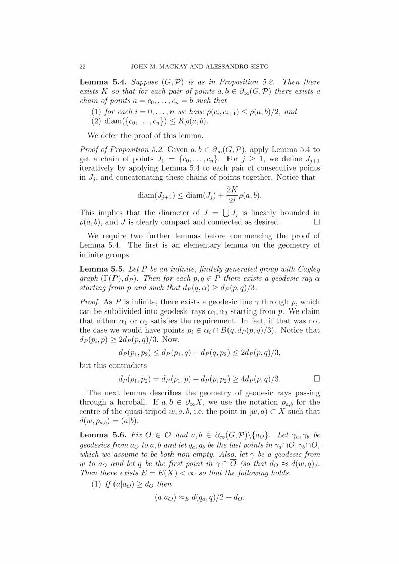
Lemma 5.6. Fix O ∈ O and a, b ∈ ∂∞(G,P)\{aO}. Let γa, γb begeodesics from aO to a, b and let qa, qb be the last points in γa∩O, γb∩O,which we assume to be both non-empty. Also, let γ be a geodesic fromw to aO and let q be the first point in γ ∩ O (so that dO ≈ d(w, q)).Then there exists E = E(X) <∞ so that the following holds.
(1) If (a|aO) ≥ dO then
(a|aO) ≈E d(qa, q)/2 + dO.
QUASI-HYPERBOLIC PLANES IN RELATIVELY HYPERBOLIC GROUPS 23
(2) If (a|aO), (b|aO) ∈ [dO, (a|b)] then
(a|b) &E 2(a|aO)− dO − d(qa, qb)/2 ≈E d(qa, q) + dO − d(qa, qb)/2.
Moreover, if d(qa, qb) ≥ E then ≈E holds in the equation above.(3) If (a|aO) < dO then d(qa, q) ≈E 0.(4) If pa,b ∈ O and d(pa,b, X \O) ≥ R ≥ E then d(pa,aO , X \O) and
d(pb,aO , X \O) are both at least R−E, and d(qa, qb) ≥ 2R−E.
Proof. As in Lemma 3.3 we only need to make the computations in thecase of trees, illustrated by Figure 2, and an approximation argumentgives in each case the desired inequalities.
Figure 2. Geodesics passing through a horoball
(1) Keeping into account that x lies in O as d(w, x) = (a|aO) ≥ dO,the computation in a tree yields
(a|aO) = d(w, q) + d(q, x) = dO + d(qa, q)/2,
as d(x, q) = d(x, qa).(2) The figure illustrates the first of the two possible types of tree
approximating the configuration we are interested in. The second caseto consider is when qa, qb are between x and y, and thus qa = qb in thetree. Therefore, for a suitable choice of E, the “moreover” assumptionensures we are in the first case. In this first case we have the equality:
(a|b) = d(w, x)+d(q, x)−d(qa, qb)/2 = (a|aO)+((a|aO)−dO)−d(qa, qb)/2.
In the second case we can proceed similarly. We see that
(a|b) ≥ d(w, qa) = d(w, x) + d(x, qa)
= (a|a0) + ((a|aO)− dO) = 2(a|aO)− dO,
which is what we need as d(qa, qb) = 0. In both cases the final ≈ followsfrom part (1).
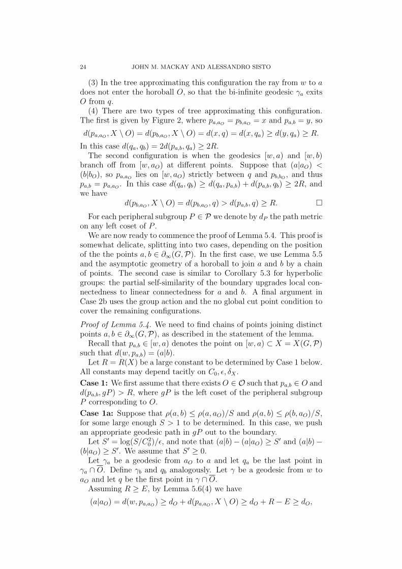
24 JOHN M. MACKAY AND ALESSANDRO SISTO
(3) In the tree approximating this configuration the ray from w to adoes not enter the horoball O, so that the bi-infinite geodesic γa exitsO from q.
(4) There are two types of tree approximating this configuration.The first is given by Figure 2, where pa,aO = pb,aO = x and pa,b = y, so
d(pa,aO , X \O) = d(pb,aO , X \O) = d(x, q) = d(x, qa) ≥ d(y, qa) ≥ R.
In this case d(qa, qb) = 2d(pa,b, qa) ≥ 2R.The second configuration is when the geodesics [w, a) and [w, b)
branch off from [w, aO) at different points. Suppose that (a|aO) <(b|bO), so pa,aO lies on [w, aO) strictly between q and pb,bO , and thuspa,b = pa,aO . In this case d(qa, qb) ≥ d(qa, pa,b) + d(pa,b, qb) ≥ 2R, andwe have
d(pb,aO , X \O) = d(pb,aO , q) > d(pa,b, q) ≥ R. �
For each peripheral subgroup P ∈ P we denote by dP the path metricon any left coset of P .
We are now ready to commence the proof of Lemma 5.4. This proof issomewhat delicate, splitting into two cases, depending on the positionof the the points a, b ∈ ∂∞(G,P). In the first case, we use Lemma 5.5and the asymptotic geometry of a horoball to join a and b by a chainof points. The second case is similar to Corollary 5.3 for hyperbolicgroups: the partial self-similarity of the boundary upgrades local con-nectedness to linear connectedness for a and b. A final argument inCase 2b uses the group action and the no global cut point condition tocover the remaining configurations.
Proof of Lemma 5.4. We need to find chains of points joining distinctpoints a, b ∈ ∂∞(G,P), as described in the statement of the lemma.
Recall that pa,b ∈ [w, a) denotes the point on [w, a) ⊂ X = X(G,P)such that d(w, pa,b) = (a|b).
Let R = R(X) be a large constant to be determined by Case 1 below.All constants may depend tacitly on C0, ε, δX .
Case 1: We first assume that there existsO ∈ O such that pa,b ∈ O andd(pa,b, gP ) > R, where gP is the left coset of the peripheral subgroupP corresponding to O.
Case 1a: Suppose that ρ(a, b) ≤ ρ(a, aO)/S and ρ(a, b) ≤ ρ(b, aO)/S,for some large enough S > 1 to be determined. In this case, we pushan appropriate geodesic path in gP out to the boundary.
Let S ′ = log(S/C20)/ε, and note that (a|b)− (a|aO) ≥ S ′ and (a|b)−
(b|aO) ≥ S ′. We assume that S ′ ≥ 0.Let γa be a geodesic from aO to a and let qa be the last point in
γa ∩ O. Define γb and qb analogously. Let γ be a geodesic from w toaO and let q be the first point in γ ∩O.
Assuming R ≥ E, by Lemma 5.6(4) we have
(a|aO) = d(w, pa,aO) ≥ dO + d(pa,aO , X \O) ≥ dO +R− E ≥ dO,
QUASI-HYPERBOLIC PLANES IN RELATIVELY HYPERBOLIC GROUPS 25
and likewise (b|aO) ≥ dO. Using Lemma 5.6(1) and the approximateequality case of Lemma 5.6(2), we have
d(qa, q) ≈2E 2((a|aO)− dO)
≥ 2((a|aO)− dO)) + 2(S ′ − (a|b) + (a|aO))
= 2(2(a|aO)− (a|b)− dO + S ′) ≈2E d(qa, qb) + 2S ′.
(5.7)
We now define our chain of points joining a to b. Let α be a geodesicin gP connecting qa to qb, and denote by qa = q0, . . . , qn = qb thepoints of α ∩ gP . For i = 0, . . . , n − 1 let ci = qiq
−10 a ∈ ∂∞(G,P) be
the endpoint of qiq−10 γa other than aO, and set cn = b. Notice that
2 log(dP (q, qa)/dP (qa, qb)) ≈2A d(q, qa)− d(qa, qb) &4E 2S ′
by Lemma 2.7 and (5.7), so for S = S(E,A) large enough,
2 log(dP (q, qa)/dP (qa, qb)− 1) ≥ S ′,
thus
d(q, qi) ≈A 2 log(dP (q, qi)) ≥ 2 log(dP (q, qa)− dP (qa, qi))
≥ 2 log(dP (q, qa)− dP (qa, qb))
≥ S ′ + 2 log(dP (qa, qb)) ≈A S ′ + d(qa, qb).
In particular, if S = S(E,A) is large enough we have (ci|aO) ≥ dO foreach i, by Lemma 5.6(3). By Lemma 2.7, as dP (qa, qi) ≤ dP (qa, qb) wehave d(qa, qi) .2A d(qa, qb). Thus Lemma 5.6(2) gives
(a|ci) &E 2(a|aO)− dO − d(qa, qi)/2
&A 2(a|aO)− dO − d(qa, qb)/2 ≈E (a|b),
which gives the distance bound ρ(a, ci) ≤ C1ρ(a, b), for C1 = C1(E,A).This gives the diameter bound diam({ci}) ≤ K1ρ(a, b) for K1 = 2C1.
We saw that (a|ci) &2E+A (a|b) ≥ S ′ + (a|aO), and so (ci|aO) &min{(ci|a), (a|aO)} & (a|aO), with error C2 = C2(E,A). We also have(ci|ci+1) &1 d(q, qi) + dO ≈E (ci|aO) + 1
2d(q, qi) &A (ci|aO) + 1
2S ′, so for
S = S(E,A) large enough, (ci|ci+1) ≥ (ci|aO) and likewise (ci|ci+1) ≥(ci+1|aO). Applying Lemma 5.6(2) twice and Lemma 5.6(4) we see that
(ci|ci+1) &E 2(ci|aO)− dO − d(qi, qi+1)/2 &2C2+1 2(a|aO)− dO≈E (a|b) + d(qa, qb)/2 &E (a|b) +R,
and so for R ≥ R1(C2, E) we have ρ(ci, ci+1) ≤ ρ(a, b)/2.
Case 1b: Suppose that b = aO. In this case, a chain of points joining aand aO is found by using an appropriate geodesic ray in gP and pushingit out to the boundary. For a suitable choice of R, depending on thevalue of S fixed by Case 1a, we will actually ensure that the distancebetween subsequent points in the chain is at most ρ(a, aO)/2(S + 1).
26 JOHN M. MACKAY AND ALESSANDRO SISTO
Let γa, qa, γ and q be as above. Notice that q, qa lie on gP , so byLemma 5.6(1)
(5.8) (a|aO) ≈E d(qa, q)/2 + dO ≥ R + dO.
By Lemma 5.5, there exists a geodesic ray α in gP starting at qasuch that dP (q, α) ≥ dP (qa, q)/3. Therefore, by Lemma 2.7 and (5.8),(5.9)d(q, α) ≈A 2 log(dP (q, α)) ≥ 2 log(dP (qa, q)/3) ≈A+3 d(qa, q) ≥ 2R.
Let qa = q0, . . . , qn, . . . be the points of α∩gP , and, as before, for eachi ≥ 0 let ci = qiq
−10 γa ∈ ∂∞(G,P).
By Lemma 5.6(3) and (5.9), for R ≥ R2(E,A) ≥ R1, we can assumethat (ci|aO) ≥ dO for each i.
Using Lemma 5.6(1) and (5.9), there exists C3 = C3(A) so that
(ci|aO) ≈E d(qi, q)/2 + dO &C3 d(qa, q)/2 + dO ≈E (a|aO).
And consequently there exists C4 = C4(C3, E) so that for each i
(5.10) ρ(ci, aO) ≤ C4ρ(a, aO);
this gives diam({ci}) ≤ K2ρ(a, aO) for K2 = 2C4.Similarly to Case 1a, we have (ci|ci+1) &1+E (ci|aO) + 1
2d(q, qi) and
d(q, qi) &2A+3 2R, so for R ≥ R3(E,A) ≥ R2 we have (ci|ci+1) ≥max{(ci|aO), (ci+1|aO)}. By Lemma 5.6(2), (5.8) and (5.9), we havefor C5 = C5(A)
(ci|ci+1) &E d(qi, q) + dO − d(qi, qi+1)/2 &C5 d(qa, q) + dO
=(d(qa, q)/2 + dO
)+ d(qa, q)/2 &E (a|aO) +R.
So, taking R ≥ R4(C5, E, S) ≥ R3, we have
(5.11) ρ(ci, ci+1) ≤ ρ(a, aO)/2(S + 1).
For each i, by Lemmas 2.7 and 5.6(1), (ci|aO) ≈E+A log(dP (qi, q)) +dO, so for N large enough we have ρ(cN , a) ≤ ρ(a, aO)/2(S + 1).
Therefore the chain of points a = c0, . . . , cN , aO = b satisfies ourrequirements by (5.10), (5.11).
Case 1c: In this case, we have ρ(a, b) ≥ ρ(a, aO)/S or ρ(a, b) ≥ρ(b, aO)/S. Without loss of generality, we assume that ρ(a, aO) ≤ρ(b, aO) and ρ(a, aO) ≤ Sρ(a, b).
Assume that R ≥ R5 = R4 +E. Then by Lemma 5.6(4), d(pa,aO , X \O) and d(pb,aO , X \ O) are both at least R4, so by Case 1b there existchains a = c0, c1, . . . , cm = aO and aO = c′0, c
′1, . . . c
′n = b, with, for each
i,
ρ(ci, ci+1) ≤ ρ(a, aO)
2(S + 1)≤ Sρ(a, b)
2(S + 1)<ρ(a, b)
2, and
ρ(c′i, c′i+1) ≤ ρ(b, aO)
2(S + 1)≤ ρ(b, a) + ρ(a, aO)
2(S + 1)≤ ρ(a, b)
2.
QUASI-HYPERBOLIC PLANES IN RELATIVELY HYPERBOLIC GROUPS 27
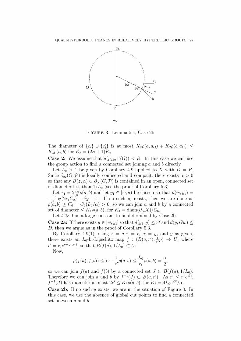
Figure 3. Lemma 5.4, Case 2b
The diameter of {ci} ∪ {c′i} is at most K2ρ(a, aO) + K2ρ(b, aO) ≤K3ρ(a, b) for K3 = (2S + 1)K2.
Case 2: We assume that d(pa,b,Γ(G)) < R. In this case we can usethe group action to find a connected set joining a and b directly.
Let L0 > 1 be given by Corollary 4.9 applied to X with D = R.Since ∂∞(G,P) is locally connected and compact, there exists α > 0so that any B(z, α) ⊂ ∂∞(G,P) is contained in an open, connected setof diameter less than 1/L0 (see the proof of Corollary 5.3).
Let r1 = 2L0
αρ(a, b) and let y1 ∈ [w, a) be chosen so that d(w, y1) =
−1ε
log(2r1C0) − δX − 1. If no such y1 exists, then we are done asρ(a, b) ≥ C6 = C6(L0/α) > 0, so we can join a and b by a connectedset of diameter ≤ K4ρ(a, b), for K4 = diam(∂∞X)/C6.
Let t� 0 be a large constant to be determined by Case 2b.
Case 2a: If there exists y ∈ [w, y1] so that d(y1, y) ≤ 3t and d(y,Gw) ≤D, then we argue as in the proof of Corollary 5.3.
By Corollary 4.9(1), using z = a, r = r1, x = y1 and y as given,there exists an L0-bi-Lipschitz map f : (B(a, r′), 1
r′ρ) → U , where
r′ = r1eεd(y1,y′), so that B(f(a), 1/L0) ⊂ U .
Now,
ρ(f(a), f(b)) ≤ L0 ·1
r′ρ(a, b) ≤ L0
r1
ρ(a, b) =α
2,
so we can join f(a) and f(b) by a connected set J ⊂ B(f(a), 1/L0).Therefore we can join a and b by f−1(J) ⊂ B(a, r′). As r′ ≤ r1e
ε3t,f−1(J) has diameter at most 2r′ ≤ K5ρ(a, b), for K5 = 4L0e
ε3t/α.
Case 2b: If no such y exists, we are in the situation of Figure 3. Inthis case, we use the absence of global cut points to find a connectedset between a and b.
28 JOHN M. MACKAY AND ALESSANDRO SISTO
Let y2 ∈ [w, y1) be chosen so that d(y1, y2) = t and let O ∈ O bethe horoball containing [y2, y1], which corresponds to the coset gP . LetdO = d(w,O), and let p1 ∈ gP be chosen so that d(p1, pa,b) < R. (Inthe figure, p1 = pa,b.)
Let ρ1 be a visual metric on ∂∞X = ∂∞(G,P) based at p1. We canassume that (∂∞X, ρ) and (∂∞X, ρ1) are isometric, with the isometryinduced by the action of p1. In the metric ρ1, we have that a, b and aOare points separated by at least δ0 = δ0(R).
The boundary (∂∞X, ρ) = (∂∞X, ρ1) is compact, locally connectedand connected. Consequently, given a point c ∈ ∂∞X that is not aglobal cut point, and δ0 > 0, there exists δ1 = δ1(δ0, c, ∂∞X) > 0so that any two points in ∂∞X \ B(c, δ0) can be joined by an arc in∂∞X \B(c, δ1).
In our situation, δ1 may be chosen to be independent of the choiceof (finitely many) c = aO satisfying d(O, p1) = 0, so δ1 = δ1(δ0, ∂∞X).Therefore, a and b can be joined by a compact arc J in (∂∞X, ρ1) thatdoes not enter Bρ1(aO, δ1). So geodesic rays from p1 to points in J areat least 2δX from the geodesic ray [pa,b, aO) outside the ball B(p1, t),for t = −1
εlog(δ1) + C7, where C7 = C7(C0, ε, δX , R).
Translating this back into a statement about (∂∞X, ρ), we see thatgeodesics from w to points in J must branch from [w, pa,b] after y2, thatis, the set J lies in the ballB(a, (K6/2)ρ(a, b)), forK6 = K6(d(pa,b, y2)) =K6(r1, t).
From these connected sets of controlled diameter, it is easy to extractchains of points satisfying the conditions of the lemma, with K =max{K1, . . . , K6}. �
6. Avoidable sets in the boundary
In order to build a hyperbolic plane that avoids horoballs, we needto build an arc in the boundary that avoids parabolic points. In Theo-rem 1.3, we also wish to avoid the specified hyperbolic subgroups. Wehave topological conditions such as the no local cut points conditionwhich help, but in this section we find more quantitative control.
Given p ∈ X, and 0 < r < R, the annulus A(p, r, R) is defined to beB(p,R) \B(p, r). More generally, we have the following.
Definition 6.1. Given a set V in a metric space Z, and constants0 < r < R <∞, we define the annular neighbourhood
A(V, r, R) = {z ∈ Z : r ≤ d(z, V ) ≤ R}.
If an arc passes through (or close to) a parabolic point in the bound-ary, we want to reroute it around that point. The following definitionwill be used frequently in the following two sections.
QUASI-HYPERBOLIC PLANES IN RELATIVELY HYPERBOLIC GROUPS 29
Definition 6.2 ([Mac08]). For any x and y in an embedded arc A,let A[x, y] be the closed, possibly trivial, subarc of A that lies betweenthem.
An arc B ι-follows an arc A, for some ι ≥ 0, if there exists a (notnecessarily continuous) map p : B → A, sending endpoints to end-points, such that for all x, y ∈ B, B[x, y] is in the ι-neighbourhood ofA[p(x), p(y)]; in particular, p displaces points at most ι.
We now define our notion of avoidable set, which is a quantitativelycontrolled version of the no local cut point and not locally disconnectingconditions.
Definition 6.3. Suppose (X, d) is a complete, connected metric space.A set V ⊂ X is L-avoidable on scales below δ for L ≥ 1, δ ∈ (0,∞]if for any r ∈ (0, δ/2L), whenever there is an arc I ⊂ X and pointsx, y ∈ I ∩ A(V, r, 2r) so that I[x, y] ⊂ N(V, 2r), there exists an arcJ ⊂ A(V, r/L, 2rL) with endpoints x, y so that J (4rL)-follows I[x, y].
The goal of this section is the following proposition.
Proposition 6.4. Let (G,P1) and (G,P1∪P2) be relatively hyperbolicgroups, where all groups in P2 are proper infinite hyperbolic subgroupsof G (P2 may be empty), and all groups in P1 are proper, finitely pre-sented and one-ended. Let X = X(G,P1), and let H be the collectionof all horoballs of X and left cosets of the subgroups of P2. (As usualwe regard G as a subspace of X.)
Suppose that ∂∞X is connected and locally connected, with no globalcut points. Suppose that ∂∞P does not locally disconnect ∂∞X foreach P ∈ P2. Then there exists L ≥ 1 so that for every H ∈ H,∂∞H ⊂ ∂∞X is L-avoidable on scales below e−εd(w,H).
This proposition is proved in the following two subsections.
6.1. Avoiding parabolic points. We prove Proposition 6.4 in thecase H is a horoball. This is the content of the following proposition.
Proposition 6.5. Suppose (G,P) is relatively hyperbolic, ∂∞(G,P)is connected and locally connected with no global cut points, and allperipheral subgroups are one-ended and finitely presented. Then thereexists L ≥ 1 so that for any horoball O ∈ O, aO = ∂∞O ∈ ∂∞(G,P) isL-avoidable on scales below e−εd(w,O).
The reason for restricting to this scale is that this is where the geom-etry of the boundary is determined by the geometry of the peripheralsubgroup. Recall from Proposition 4.3 that such parabolic points arenot local cut points.
The first step is the following simple lemma about finitely presented,one-ended groups. It essentially states that we can join two large el-ements of such a group without going too close or too far from the
30 JOHN M. MACKAY AND ALESSANDRO SISTO
identity. Near a parabolic point, this allows us to prove Proposition 6.5by joining two suitable points without going to far from or close to theparabolic point.
Lemma 6.6. Suppose P is a finitely generated, one-ended group, givenby a (finite) presentation where all relators have length at most M , andlet Γ(P ) be its Cayley graph. Then any two points x, y ∈ Γ(P ) such that2M ≤ rx ≤ ry, where rx = d(e, x) and ry = d(e, y), can be connectedby an arc in A(e, rx/3, 2ry) ⊂ Γ(P ).
Proof. By Lemma 5.5, we can find an infinite geodesic ray in Γ(P ) fromx which does not pass through B(e, rx/3). Let x′ be the last point onthis ray satisfying d(e, x′) = ry. Do the same for y, and let y′ denotethe corresponding point. Note that x′ and y′ lie on the boundary ofthe unique unbounded component of {z ∈ Γ(P ) : d(e, z) ≥ ry}, whichwe denote by Z. We prove the lemma by finding a path from x′ to y′
contained in A(e, ry −M, ry +M).Let β1 be an arc joining x′ and y′ in Z. It suffices to consider the
case when β1∩B(e, ry) = {x′, y′}. Let p be the first point of [y′, e] thatmeets [e, x′] in Γ(P ). Then the concatenation of β1, [y
′, p] and [p, x′]forms a simple, closed loop β2 in Γ(P ).
As β2 represents the identity in P , there exists a diagram D for β2: aconnected, simply connected, planar 2-complex D together with a mapof D into the Cayley complex Γ2(P ) sending cells to cells and ∂D toβ2.
Let D′ ⊂ D be the union of closed faces B ⊂ D which have a pointu ∈ ∂B with d(u, e) = ry. Let D′′ be the connected component of x′ inD′. Let γ : S1 → ∂D′′ be the outer boundary path of D′′ ⊂ R2.
If either β1 or [y′, p]∪ [p, x′] live in A(p, ry−M, ry +M), we are done.Otherwise, as we travel around γ from x′, in one direction we musttake a value > ry, and in the other a value < ry, thus there is a pointv ∈ γ \ {x′} with d(e, v) = ry. If v is in the interior of D, the adjacentfaces are in D′, giving a contradiction. So v ∈ β2, and v must be y′.Thus there is a path from x′ to y′ in D′ ⊂ A(e, ry −M, ry +M). �
We can now prove the proposition. The idea is similar to Lemma 5.4,Case 1: we find a suitable path using Lemma 6.6 and push it out to∂∞X.
Proof of Proposition 6.5. By Proposition 4.3, parabolic points in theboundary are not local cut points.
We claim that there exists an L ≥ 1 so that for any parabolic pointaO, any r ≤ e−εd(w,O)/2L, and any a, b ∈ A(aO, r, 2r), there exists anarc J ⊂ A(aO, r/L, 2rL) joining a to b.
This claim suffices to prove the proposition, because the 4rL-followingproperty automatically follows from diam(B(aO, 2rL)) ≤ 4rL. We nowproceed to prove the claim.
QUASI-HYPERBOLIC PLANES IN RELATIVELY HYPERBOLIC GROUPS 31
Using the notation of Lemma 5.6, let gP be the left coset of a pe-ripheral group that corresponds to O, and let q ∈ gP be the first pointof [w, aO) in O. Recall that dO = d(w,O) ≈ d(w, q). Let qa, qb be thelast points of (aO, a), (aO, b) contained in O.
We begin by describing the positions of q, qa and qb in the pathmetric dP on gP ⊂ X. We write x �C y if the quantities x, y satisfyx/C ≤ y ≤ Cx.
Sincee−ε(a|aO) �C0 ρ(a, aO) �2 r ≤ e−εdO/2L,
we have, for some C1 = C1(C0, ε),
(a|aO) ≈C1 log(r−1/ε) ≥ dO + log(2L)/ε,
so for L ≥ L(C1, ε), we have (a|aO) ≥ dO, and likewise (b|aO) ≥ dO.Lemmas 2.7 and 5.6(1), with A and E as before, give
(6.7) 2 log(dP (qa, q)) ≈A d(qa, q) ≈2E 2((a|aO)− dO)
≈2C1 2 log(r−1/εe−dO) ≥ 2 log(2L)/ε,
so dP (qa, q) �C2 r−1/εe−dO , for C2 = C2(A,E,C1). Let rP be thesmaller of dP (qa, q), dP (qb, q), and notice that the larger value is atmost C2
2rP .We now use Lemma 6.6 to find a chain of points qa = q0, q1, . . . , qn =
qb in gP joining qa to qb in gP , so that qi ∈ A(q, rP/3, 2rPC22) in the
metric dP . Let ci = qiq−10 a, for i = 0, . . . , n − 1, and set cn = b. This
gives a chain of points {ci} in ∂∞X joining a to b. (Observe that wecan take (aO, ci) = qiq
−10 (aO, a).)
Lemma 2.7 and (6.7) imply that
d(qi, q) ≈ 2 log(dP (qi, q)) ≈ 2 log(dP (qa, q)) ≈ d(qa, q) & 2 log(2L)/ε,
with total error C3 = C3(A,E,C1, C2). So if L ≥ L(C3, ε), we haved(qi, q) > E, and therefore (ci|aO) ≥ dO by Lemma 5.6(3).
Now Lemma 5.6(1) shows that
(ci|aO) ≈E d(qi, q)/2 + dO ≈C3 d(qa, q)/2 + dO ≈E (a|aO),
so ρ(ci, aO) � ρ(a, aO) � r, with total error C4 = C4(C3, E), that isci ∈ A(aO, r/C4, C4r).
We now wish to join each ci and ci+1 in a suitable annulus aroundaO. Consider the geodesics between w, ci and ci+1, and observe thatd(qi, q) > E > δX , and dP (qi, qi+1) = 1. From this, and (6.7), we seethat
(ci|ci+1) & d(w, qi) ≈ dO + d(q, qa) ≈ 2 log(r−1/ε)− dO,and so, for suitable C5,
ρ(ci, ci+1) ≤ C0e−ε(ci|ci+1) ≤ C5r
2eεdO ≤ C5r/2L.
By Proposition 5.2, ∂∞X is L′-linearly connected, so if L ≥ C4C5L′
we can join ci to ci+1 in B(ci, L′C5r/2L) ⊂ B(ci, r/2C4). Since ci ∈
32 JOHN M. MACKAY AND ALESSANDRO SISTO
A(aO, r/C4, C4r) we have joined ci to ci+1 in A(aO, r/2C4, 2C4r), andthe claim follows. �
6.2. Avoiding hyperbolic subgroups. In this section we completethe proof of Proposition 6.4 for H = gP , where P ∈ P2. By assump-tion, ∂∞H ⊂ ∂∞X does not locally disconnect ∂∞X.
First, we show that boundaries of peripheral groups are porous.
Definition 6.8 (e.g. [Hei01, 14.31]). A set V in a metric space (Z, ρ)is C-porous on scales below δ if for any z ∈ V and 0 < r < δ, thereexists z′ ∈ B(z, r) so that ρ(z′, V ) ≥ r/C.
Lemma 6.9. Under the assumptions of Proposition 6.4, there existsL1 so that for every H ∈ H, ∂∞H ⊂ ∂∞X is L1-porous on scales belowe−εd(w,H).
The proof follows from the partial self-similarity of Corollary 4.9 andthe fact that for any H ∈ H, ∂∞H has empty interior in ∂∞X.
Proof. Observe that if H is a horoball, then ∂∞H is a point in a con-nected space, and so is automatically porous.
If the conclusion is false, we can find a sequence of cosets Hn = gnPn,for Pn ∈ P2, points an ∈ ∂∞Hn and values rn ≤ e−εd(w,Hn) so thatN(∂∞Hn, rn/n) ⊃ B(an, rn).
Let drn ≈ log(r−1/εn ) be given as in Corollary 4.9 with z = an, r = rn.
Assume that we can take a subsequence and reindex so that drn ≥ 0for all n. Let xn ∈ [w, an) be the point satisfying d(w, xn) = drn .Every H ∈ H is uniformly quasi-convex, see Lemma 3.1(2), and rn ≤e−εd(w,Hn), so d(xn, Hn) is uniformly bounded for any such xn. Thereforethere exists hn ∈ G so that d(h−1
n w, xn) ≤ D, for some uniform constantD.
Thus Corollary 4.9 implies that there exists L0 = L0(D) and L0-bi-Lipschitz maps fn : (B(an, rn), 1
rnρ) → ∂∞X induced by the action of
hn, so that B(fn(an), 1/L0) ⊂ fn(B(an, rn)).As hnHn = H ′n for someH ′n ∈ H, and d(H ′n, w) is uniformly bounded,
we may take a subsequence so that H ′n = H ′ ∈ H for all n, andmoreover that fn(an) ∈ ∂∞H ′ converges to a ∈ ∂∞H ′. Therefore, forall sufficiently large n,
B(a, 1/2L0) ⊂ B(fn(an), 1/L0) ⊂ fn(B(an, rn))
= fn(B(an, rn) ∩N(∂∞Hn, rn/n)) ⊂ N(∂∞H′, L0/n),
so a is in the interior of ∂∞H′ ⊂ ∂∞X, since ∂∞H
′ is closed in ∂∞X.This is a contradiction because ∂∞H
′ is not all of ∂∞X (proper periph-eral subgroups of a relatively hyperbolic group are of infinite index),so if a is a point of ∂∞H
′, one can use the action of H ′ to find pointsin ∂∞X \ ∂∞H ′ that are arbitrarily close to a.
There remains the case where infinitely many drn < 0. But then forsuch a subsequence we have all rn > C > 0, and d(e,Hn) is uniformly
QUASI-HYPERBOLIC PLANES IN RELATIVELY HYPERBOLIC GROUPS 33
bounded. Therefore we can proceed as above to take a subsequenceso that Hn = H ′ for all n and B(fn(an), C) ⊂ N(∂∞Hn, rn/n) ⊂N(∂∞H
′, 1/n). The rest of the argument is the same. �
We continue with the proof of Proposition 6.4. The basic idea is touse partial self-similarity and a compactness argument to upgrade thetopological condition of not locally disconnecting to the quantitativeL-avoidable condition.
We begin with the following lemma.
Lemma 6.10. Given L1 ≥ 1, there exists L2 = L2(X,L1) independentof H = gP , P ∈ P2, so that for any r ≤ e−εd(w,H)/L2, and any twopoints u, v ∈ A(∂∞H, r/L1, 2r) so that ρ(u, v) ≤ 4r, there exists an arc
K ⊂ A(∂∞H, r/L2, 2L2r)
joining u to v with diam(K) ≤ 2L2r.
Proof. As in Lemma 6.9, we assume the conclusion is false, and willuse self-similarity to derive a contradiction.
If the conclusion is false, there is a sequence of Hn = gnPn withPn ∈ P2, rn ≤ e−εd(w,Hn)/n, and points an ∈ ∂∞Hn and un, vn ∈B(an, 6rn)∩A(∂∞Hn, rn/L1, 2rn) so that there is no arc of diameter atmost 2nrn joining un to vn in A(∂∞Hn, rn/n, 2nrn).
As before, the geodesic [w, an) essentially travels from w straight toHn then along Hn to an ∈ ∂∞Hn. More precisely, there are constantsC1 and D depending on the uniform quasi-convexity constant of Hn
and δX so that for any r ≤ e−εd(w,Hn)/C1, the point x, defined byCorollary 4.9(1) applied to z = an and r, lies within distance D of Gw.Let L0 = L0(D) be the corresponding constant from Corollary 4.9.
Let L′ be the linear connectivity constant of ∂∞X, and set r′n =10L2
0L′rn. For n large enough, r′n ≤ e−εd(w,Hn)/C1, and so we find hn ∈
G that induces a L0-bi-Lipschitz map fn : (B(an, r′n), 1
r′nρ) → ∂∞X,
with B(fn(an), 1/L0) ⊂ fn(B(an, r′n)). Note that hn maps Hn to some
H ′n ∈ H, with fn(an) ∈ ∂∞H ′n. As d(w,H ′n) is uniformly bounded, wecan take a subsequence so that H ′n = H ′ ∈ H.
The images fn(un), fn(vn) lie in B(fn(an), T ) \ N(∂∞H′, t), where
T = 6rnL0/r′n < 1/L0L
′ and t = rn/r′nL1L0 are independent of n. Let
W = {(u, v, a) : a ∈ ∂∞H ′, {u, v} ⊂ B(a, T ) \N(∂∞H′, t)} ⊂ (∂∞X)3,
and define f : W → (0, T ] to be supremal so that for (u, v, a) ∈ Wthere exists an arc joining u to v in B(a, 1/L0) \ N(∂∞H
′, f(u, v, a)).We know that f is positive because for any (u, v, a) ∈ W , B(a, T ) liesin a connected open set U ⊂ B(a, 1/L0), and as ∂∞H
′ does not locallydisconnect, U \ ∂∞H ′ is connected and we can join u to v in this set.
Observe that by local connectivity f is continuous, and W is com-pact, so f(u, v, a) ≥ 2C2 > 0 for some C2 and all (u, v, a) ∈ W .
34 JOHN M. MACKAY AND ALESSANDRO SISTO
Now (fn(un), fn(vn), fn(an)) ∈ W , so there exists an arc K join-ing fn(un) to fn(vn) with K ′ ⊂ B(fn(an), 1/L0) \ N(∂∞H
′, C2). Thepreimage K = f−1
n (K ′) joins un to vn so that
K ⊂ B(an, r′n) ∩ A(∂∞H, r
′nC2/L0, r
′n),
which is a contradiction for large enough n. �
We now finish the proof of Proposition 6.4, fixing constants L1 ≥ 2from Lemma 6.9 and L2 = L2(X,L1) from Lemma 6.10.
LetH = gP , P ∈ P2 be fixed. Suppose we are given r ≤ e−εd(w,H)/L2,points x, y ∈ A(∂∞H, r, 2r), and an arc I ⊂ N(H, 2r) with endpointsx and y.
We build our desired arc J from x to y in stages. First, let x =z′0, z
′1, . . . , z
′m = y be a (finite) chain of points that 0-follows I[x, y], so
that ρ(zi, zi+1) ≤ r. (The definition of ι-follows is extended from arcsto chains in the obvious way.) For each i, if ρ(z′i, ∂∞H) ≤ r/L1, useLemma 6.9 to find a point zi at most r/L1+r away from z′i, and outsideN(∂∞H, r/L1). Otherwise let zi = z′i.
This new chain satisfies {zi} ⊂ A(∂∞H, r/L1, 2r), and for every i,ρ(zi, zi+1) ≤ r + 2(r/L1 + r) ≤ 4r. It 2r-follows {z′i}, and thus {zi}also 2r-follows I.
By Lemma 6.10 for each i there exist an arc Ji joining zi and zi+1
which lies in A(∂∞H, r/L2, 2L2r) and has diam(Ji) ≤ 2L2r. From this,we extract an arc J by cutting out loops: travel along J0 until youmeet Jj for some j ≥ 1, and at that point cut out the rest of J0 and allJk for 1 ≤ k < j. Concatenate the remainders of J0 and Jj together,and continue along Jj.
The resulting arc J will 2L2r-follow the chain {zi}, and so it will4L2r-follow I as desired. �
7. Quasi-arcs that avoid obstacles
A quasi-arc is a metric space which is quasisymmetrically homeo-morphic to [0, 1] with its usual metric. Tukia and Vaisala showed thatone can equivalently define a quasi-arc as a metric space which is atopological arc, and which is doubling and linearly connected [TV80,Theorem 4.9]. (If this arc is λ-linearly connected, we call the arc aλ-quasi-arc.)
As discussed in the introduction, Tukia showed that doubling andlinearly connected metric spaces contain quasi-arcs joining any twopoints [Tuk96, Theorem 1A].
In this section we build quasi-arcs in a metric space that avoid spec-ified obstacles. This result can be viewed from the perspective of Dio-phantine approximation for finite volume hyperbolic manifolds; see Ex-ample 7.6. The methods we use build on the alternative proof of Tukia’stheorem found in [Mac08].
QUASI-HYPERBOLIC PLANES IN RELATIVELY HYPERBOLIC GROUPS 35
7.1. Collections of obstacles. The next definition gives us controlon a collection of obstacles.
Definition 7.1. Let (Z, ρ) be a compact metric space. Let V be acollection of compact subsets of Z provided with some map D : V →(0,∞), which we call a scale function.
The (modified) relative distance function ∆ : V × V → [0,∞) isdefined for V1, V2 ∈ V as
∆(V1, V2) =ρ(V1, V2)
min{D(V1), D(V2)}.
We say V is L-separated if for all V1, V2 ∈ V, if V1 6= V2 then ∆(V1, V2) ≥1L
.
As we saw in Section 6, we often only have control on topologyon a sufficiently small scale. The purpose of the scale function is todetermine the size of the neighbourhood of each V ∈ V on which wehave this control. An example of a scale function is D(V ) = diam(V ),if every V ∈ V has |V | > 1. In this case, ∆ is precisely the usualrelative distance function, e.g. [Hei01, page 59].
The goal of this section is the following result.
Theorem 7.2. Let (Z, ρ) be an N-doubling, L-linearly connected, com-pact metric space, and L ≥ 10, N ≥ 1 constants. Suppose V is anL-separated collection of compact subsets of Z with scale function D :V → (0,∞), so that V ∈ V is L-porous and L-avoidable on scales belowD(V ) (see Definitions 6.8 and 6.3).
For any ν ≥ 1 there exists a constant λ = λ(N,L, ν) so that givenany two points x, y ∈ Z, if for all V ∈ V we have ρ({x, y}, V ) ≥D(V )/ν, then x and y can be joined by a λ-quasi-arc which satisfiesρ(γ, V ) ≥ 1
λD(V ) for each V ∈ V.
The following result shows that such endpoints exist.
Proposition 7.3. Let (Z, ρ) be a compact metric space, and L ≥ 10,N ≥ 1 constants. Suppose V is an L-separated collection of compactsubsets of Z with scale function D : V → (0,∞), and suppose that eachV ∈ V is L-porous on scales below D(V ).
For any r ≤ 1/5L, given p ∈ Z there exists q ∈ Z so that ρ(p, q) ≤diam(Z)r, and that for all V ∈ V we have ρ(q, V ) ≥ D(V )r/8L2.
For the remainder of this paper we will use the following corollaryto Theorem 7.2.
Corollary 7.4. Let (Z, ρ) be a compact, N-doubling and L-linearlyconnected metric space. Suppose V is an L-separated collection of com-pact subsets of Z with scale function D : V → (0,∞), and that eachV ∈ V is both L-porous and L-avoidable on scales below D(V ).
36 JOHN M. MACKAY AND ALESSANDRO SISTO
Then for a constant λ = λ(N,L) there exists a λ-quasi-arc γ in Zwhich satisfies diam(γ) ≥ 1
2diam(Z), and ρ(γ, V ) ≥ 1
λD(V ) for each
V ∈ V.
Proof of Corollary 7.4. Let x′ and y′ be two points at maximum dis-tance in Z. Apply Proposition 7.3 with r = 1/5L to x′ and y′ tofind points x and y which are at least diam(Z)/2 apart, and haveρ({x, y}, V ) ≥ D(V )/40L3 for any V ∈ V . The corollary then followsfrom Theorem 7.2. �
Two simple applications of Corollary 7.4 are the following.
Example 7.5. Let Z be the usual square Sierpinski carpet in the plane,with Euclidean metric dEuc, and let V be the set of peripheral squares,i.e., boundaries of [0, 1]2, [1/3, 2/3]2, and so on. Define D(V ) =diam(V ) for each V ∈ V.
The assumptions of Corollary 7.4 are satisfied for suitable N andL, so there exists some λ and a λ-quasi-arc γ in Z which satisfiesdEuc(γ, V ) ≥ 1
λdiam(V ) for each V ∈ V.
It is not immediately obvious that there exists a point satisfying thislast separation condition, let alone a quasi-arc, although in the carpetit is possible to build such an arc by hand.
Example 7.6. Let M be a finite volume hyperbolic n-manifold, withn ≥ 3, and a choice of base point p ∈M . The universal cover of M isM = Hn, and fix a lift p of p. Let H be a collection of horoballs for theaction π1(M) y M = Hn.
Let Z = ∂∞Hn = Sn−1, with π1(M) acting on Z. Let V be thecollection of parabolic points ∂∞H ∈ Z, for H ∈ H, with scale functionD(H) = e−d(p,H).
Points in Sn−1 are avoidable and porous, and Sn−1 is both dou-bling and linearly connected. The linear separation of V follows fromLemma 3.2. Theorem 7.2 applies to find many quasi-arcs in Sn−1,which do not go too close to parabolic points. Moreover, geodesic raysfrom p to these quasi-arcs do not go far into horoballs by Lemma 3.3.
Identifying Sn−1 with the tangent sphere TpM , this means at anypoint p ∈ M we can find a compact subset K ⊂ M so that there arelots of (quasi-arc) paths of directions in TpM with the geodesic rays inthese directions living in K.
7.2. Building the quasi-arc. The way that Theorem 7.2 builds aquasi-arc is by an inductive process: starting with any arc in Z, pushthe arc away from the largest obstacles in V , then push it away fromthe next largest, and so on. While this is going on, one also “cuts outloops” in order to ensure the limit arc is a quasi-arc. There is somedelicacy involved in making sure the constants work out correctly.
As a warm-up, we show how to find points far from obstacles.
QUASI-HYPERBOLIC PLANES IN RELATIVELY HYPERBOLIC GROUPS 37
Proof of Proposition 7.3. If V = ∅, the result is trivial. Otherwise, letD0 = sup{D(V ) : V ∈ V}. Observe that as every V ∈ V is L-porous,we have D0 ≤ L diam(Z).
We filter V according to size. For n ∈ N, let Vn = {V ∈ V : rn <D(V )/D0 ≤ rn−1}, where r ≤ 1/5L ≤ 1/50 is given. (Recall thatL ≥ 10.) Note that N(V,D0r
n/2L)∩N(V ′, D0rn/2L) = ∅ if V and V ′
are distinct elements of Vn, because V is L-separated.Let x0 = p, and proceed by induction on n ∈ N. Suppose ρ(xn−1, V ) ≤
D0rn/4L for some (unique) V ∈ Vn. Then as V is L-porous on scales
below D(V ) > D0rn/4L, we can find xn ∈ Z so that ρ(xn−1, xn) ≤
D0rn/4L+D0r
n/4L = D0rn/2L and ρ(xn, V ) ∈ [D0r
n/4L2, D0rn/4L].
For any other V ′ ∈ Vn, we have
ρ(xn, V′) ≥ ρ(V, V ′)− ρ(V, xn) ≥ D0r
n
L− D0r
n
4L>D0r
n
4L2.
If no such V exists, set xn = xn−1. In either case, for all V ′ ∈ Vn, wehave ρ(xn, V
′) ≥ D0rn/4L2.
The sequence {xn} converges to a limit q. Observe that for anyn ≥ 0,
ρ(xn, q) ≤ ρ(xn, xn+1) + ρ(xn+1, xn+2) + · · ·
≤ D0rn+1
2L+D0r
n+2
2L+ · · · = D0r
n+1
2L(1− r).
In particular, ρ(p, q) = ρ(x0, q) ≤ D0r/2L(1− r) ≤ diam(Z)r.For any V ∈ V , there exists n so that V ∈ Vn, and we have
ρ(q, V ) ≥ ρ(xn, V )− ρ(xn, q) ≥D0r
n
4L2− D0r
n+1
2L(1− r)
=D0r
n−1r
4L2
(1− 2rL
1− r
)≥ D(V )r
8L2,
where we used that 2rL/(1− r) ≤ 1/2. �
To find quasi-arcs, we need more machinery. We now recall some ter-minology and results from [Mac08]. An arc A in a doubling and com-plete metric space is an ι-local λ-quasi-arc if diam(A[x, y]) ≤ λd(x, y)for all x, y ∈ A such that d(x, y) ≤ ι. (See Definition 6.2 for the notionof ι-following.)
Remark 7.7. Any ι-local λ-quasi-arc γ is a λ′-quasi-arc with λ′ =max{λ, diam(γ)/ι}.
Proposition 7.8 ([Mac08, Proposition 2.1]). Given a complete metricspace (Z, ρ) that is L-linearly connected and N-doubling, there existconstants s = s(L,N) > 0 and S = S(L,N) > 0 with the followingproperty: for each ι > 0 and each arc A ⊂ X, there exists an arc Jthat ι-follows A, has the same endpoints as A, and satisfies
(7.9) ∀u, v ∈ J, ρ(u, v) < sι =⇒ diam(J [u, v]) < Sι.
38 JOHN M. MACKAY AND ALESSANDRO SISTO
Lemma 7.10 ([Mac08, Lemma 2.2]). Suppose (Z, ρ) is an L-linearlyconnected, N-doubling, complete metric space, and let s, S, ε and δ befixed positive constants satisfying δ ≤ min{ s
4+2S, 1
10}. Now, if we have
a sequence of arcs J0, J1, . . . , Jn, . . . in Z, such that for every n ≥ 1
• Jn εδn-follows Jn−1, and• Jn satisfies (7.9) with ι = εδn and s, S as fixed above,
then the Hausdorff limit J = limH Jn exists, and is an εδ2-local 4S+3δδ2
-quasi-arc. Moreover, the endpoints of Jn converge to the endpoints ofJ , and J ε-follows J0.
We now use these results to build our desired quasi-arc.
Proof of Theorem 7.2. As in the proof of Proposition 7.3, let D0 =sup{D(V ) : V ∈ V}; if V = ∅, set D0 = diam(Z). Recall that D0 ≤L diam(Z), and we assume that L ≥ 10.
Let r = r(L,N, ν) > 0 be fixed sufficiently small as determined laterin the proof. As before, define Vn = {V ∈ V : rn < D(V )/D0 ≤ rn−1},for n ∈ N, and let Cn = {N(V,D0r
n/4L) : V ∈ Vn}. As V is L-separated, each Cn consists of disjoint neighbourhoods. (Note that twoneighbourhoods from different Cn may well intersect.)
Suppose x and y are given with ρ(x, V ), ρ(y, V ) ≥ D(V )/ν for eachV ∈ V . Without loss of generality, we assume that ν ≥ 10L2. LetM ∈ Z be maximal so that ρ(x, y) < D0r
M/4Lν. We start with an arcJM = JM [x, y] in Z of diameter at most Lρ(x, y), and build arcs Jn inZ by induction on n > M .
Inductive step: Assume we have been given an arc Jn−1 = Jn−1[x, y].First, assuming n > 0, we modify Jn−1 independently inside the
(disjoint) sets in Cn. Let r′n = D0rn/2ν, and observe that for any
V ∈ Vn,
A(V, r′n, 2r′n) ⊂ A(V, r′n/L, 5r
′nL) ⊂ N(V,D0r
n/4L) ∈ Cn.
Note that x and y lie outside N(V, 2r′n), as ρ({x, y}, V ) ≥ D(V )/ν >D0r
n/ν = 2r′n.Given V ∈ Vn, each time Jn−1 meets N(V, r′n/L), the arc Jn−1 travels
through A = A(V, r′n, 2r′n) both before and after meeting N(V, r′n/L).
For each such meeting, we use that V is L-avoidable with “r” equalto r′n to find a detour path in A(V, r′n/L, 2r
′nL) which 4r′nL-follows the
previous path. After doing so, we concatenate the paths found into anarc J ′n, as at the end of the proof of Proposition 6.4. This arc J ′n will4r′nL-follow Jn−1.
If n ≤ 0, set J ′n = Jn−1, which 0-follows Jn−1.Second, apply Proposition 7.8 to J ′n with ι = r′n/2L. Call the result-
ing arc Jn: it ι-follows J ′n, so it (D0rn/4L)-follows Jn−1, as ι+ 4r′nL ≤
5r′nL ≤ D0rn/4L. Since ρ(J ′n, V ) ≥ r′n/L and Jn (r′n/2L)-follows J ′n,
QUASI-HYPERBOLIC PLANES IN RELATIVELY HYPERBOLIC GROUPS 39
we also have
(7.11) ρ(Jn, V ) ≥ r′n2L
=D0r
n
4Lν.
Limit arc: Consider the sequence of arcs JM , JM+1, . . ..For every i ∈ N, JM+i (D0r
M/4L)ri-follows JM+i−1. Let s and S begiven by Proposition 7.8, then observe that JM+i satisfies ∀u, v ∈ J,
ρ(u, v) < sι =( sν
)(D0rM
4L
)ri
=⇒ diam(J [x, y]) < Sι =SD0r
M
4Lν≤ S
(D0r
M
4L
)ri.
In other words, JM+i satisfies (7.9) with s replaced by s′ = s/ν andι = (D0r
M/4L)ri.We can assume that r ≤ min
{s′
4+2S, 1
10
}, since s′ and S depend only
on L, N and ν.Now apply Lemma 7.10 to the arcs JM , JM+1, . . . with s′ replacing
s, δ = r and ε = D0rM/4L, to find an arc γ, with endpoints x and y.
The arc γ is a (D0rM+2/4L)-local µ-quasi-arc, where µ = µ(L,N, ν).
For each n ≥M , γ lies in a neighbourhood of Jn of size at most
(7.12)D0r
n+1
4L+D0r
n+2
4L+ · · · = D0r
n+1
4L(1− r)≤ D0r
n
8Lν,
where this last inequality holds for r ≤ 1/4ν. (We may now set r =min{1/4ν, s′/(4 + 2S)}.)
In particular, γ lies in a ball about x of radius at most
(7.13) diam(JM) +D0r
M
8Lν≤ Lρ(x, y) +
D0rM
8Lν≤ D0r
M
2ν,
so by Remark 7.7, γ is a λ′-quasi-arc with λ′ = λ′(L,N) the maximumof µ and diam(γ)(4L/D0r
M+2) ≤ 4L/νr2.
Avoiding obstacles: For any V ∈ Vn with n > M , (7.11) and (7.12)give
ρ(γ, V ) ≥ ρ(Jn, V )− D0rn
8Lν≥ D0r
n
8Lν≥ r
8LνD(V ).
If V ∈ Vn with n ≤ M , then ρ(x, V ) ≥ D(V )/ν ≥ D0rn/ν, while by
(7.13) γ lies in B(x,D0rM/2ν), so
ρ(γ, V ) ≥ D0rn
ν− D0r
M
2ν≥ D0r
n
2ν≥ r
2νD(V ). �
8. Building quasi-hyperbolic planes
We now have all we need to construct quasi-isometrically embeddedhyperbolic planes.
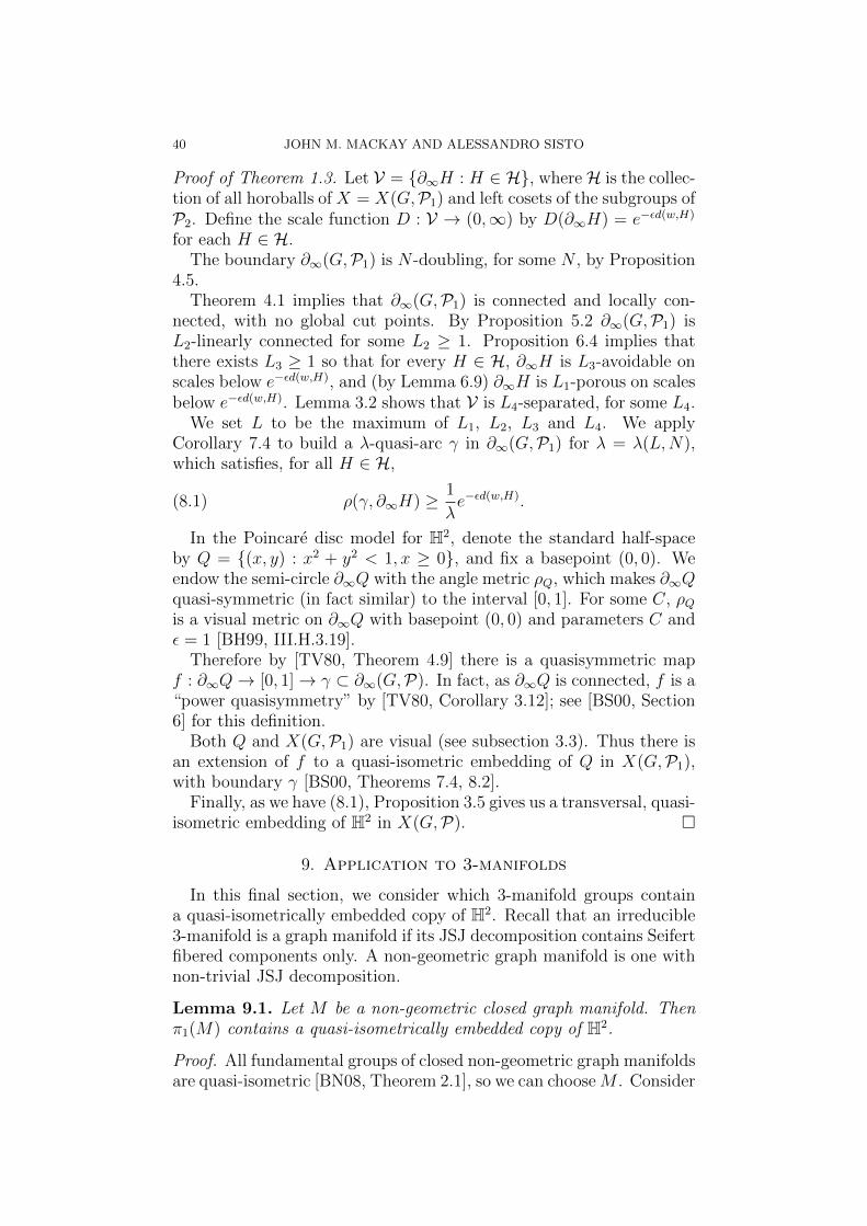
40 JOHN M. MACKAY AND ALESSANDRO SISTO
Proof of Theorem 1.3. Let V = {∂∞H : H ∈ H}, whereH is the collec-tion of all horoballs of X = X(G,P1) and left cosets of the subgroups ofP2. Define the scale function D : V → (0,∞) by D(∂∞H) = e−εd(w,H)
for each H ∈ H.The boundary ∂∞(G,P1) is N -doubling, for some N , by Proposition
4.5.Theorem 4.1 implies that ∂∞(G,P1) is connected and locally con-
nected, with no global cut points. By Proposition 5.2 ∂∞(G,P1) isL2-linearly connected for some L2 ≥ 1. Proposition 6.4 implies thatthere exists L3 ≥ 1 so that for every H ∈ H, ∂∞H is L3-avoidable onscales below e−εd(w,H), and (by Lemma 6.9) ∂∞H is L1-porous on scalesbelow e−εd(w,H). Lemma 3.2 shows that V is L4-separated, for some L4.
We set L to be the maximum of L1, L2, L3 and L4. We applyCorollary 7.4 to build a λ-quasi-arc γ in ∂∞(G,P1) for λ = λ(L,N),which satisfies, for all H ∈ H,
(8.1) ρ(γ, ∂∞H) ≥ 1
λe−εd(w,H).
In the Poincare disc model for H2, denote the standard half-spaceby Q = {(x, y) : x2 + y2 < 1, x ≥ 0}, and fix a basepoint (0, 0). Weendow the semi-circle ∂∞Q with the angle metric ρQ, which makes ∂∞Qquasi-symmetric (in fact similar) to the interval [0, 1]. For some C, ρQis a visual metric on ∂∞Q with basepoint (0, 0) and parameters C andε = 1 [BH99, III.H.3.19].
Therefore by [TV80, Theorem 4.9] there is a quasisymmetric mapf : ∂∞Q→ [0, 1]→ γ ⊂ ∂∞(G,P). In fact, as ∂∞Q is connected, f is a“power quasisymmetry” by [TV80, Corollary 3.12]; see [BS00, Section6] for this definition.
Both Q and X(G,P1) are visual (see subsection 3.3). Thus there isan extension of f to a quasi-isometric embedding of Q in X(G,P1),with boundary γ [BS00, Theorems 7.4, 8.2].
Finally, as we have (8.1), Proposition 3.5 gives us a transversal, quasi-isometric embedding of H2 in X(G,P). �
9. Application to 3-manifolds
In this final section, we consider which 3-manifold groups containa quasi-isometrically embedded copy of H2. Recall that an irreducible3-manifold is a graph manifold if its JSJ decomposition contains Seifertfibered components only. A non-geometric graph manifold is one withnon-trivial JSJ decomposition.
Lemma 9.1. Let M be a non-geometric closed graph manifold. Thenπ1(M) contains a quasi-isometrically embedded copy of H2.
Proof. All fundamental groups of closed non-geometric graph manifoldsare quasi-isometric [BN08, Theorem 2.1], so we can chooseM . Consider
QUASI-HYPERBOLIC PLANES IN RELATIVELY HYPERBOLIC GROUPS 41
a splitting of the closed genus 2 surface S into an annulus A and atwice-punctured torus S ′, as in Figure 4 below.
S
S'A
Figure 4. The surfaces S, S ′, A and the path γ.
The manifold S ′× S1 has two boundary components homeomorphicto S1 × S1. Let M be obtained from two copies M1,M2 of S ′ × S1 bygluing the corresponding boundary components together in a way thatinterchanges the two S1 factors.
We now wish to find an embedding ι of S into M so that M retractsonto the image of ι. If we have such an embedding, then first of all
π1(S) injects in π1(M), so that we get a map f : H2 → M . Also, π1(S)is undistorted in π1(M) and therefore f is a quasi-isometric embedding.
The specific embedding ι : S → M which we describe is obtainedfrom two embeddings ι1 : A→M1 and ι2 : S ′ →M2.
Let γ : [0, 1]→ S ′ be the path connecting the boundary componentsof S ′ depicted in Figure 4. As A can be identified with [0, 1] × S1 wecan define ι1 : A → M1 by (t, θ) 7→ (γ(t), θ). We can assume, up tochanging the gluings, that there exists p such that ι1(A)∩M2 ⊆ S ′×{p}.We can then define ι2 by x 7→ (x, p).
We now have an embedding ι : S → M so that ι|A = ι1, ι|S′ = ι2.We now only need to show that ι(S) is a retract of M . Define g2 :M2 → S ′ × {p} simply as (x, θ) 7→ (x, p). It is easy to see that thereexists a retraction g′ : S ′ → γ such that each boundary componentof S ′ is mapped to an endpoint of γ. Let g1 : M1 → γ × S1 be(x, θ) 7→ (g′(x), θ). There clearly exists a retraction g : M → ι(S)which coincides with gi on Mi. �
Theorem 9.2. Let M be a connected orientable closed 3-manifold.Then π1(M) contains a quasi-isometrically embedded copy of H2 if andonly if M does not split as the connected sum of manifolds each withgeometry S3,R3, S2 × R or Nil.
Proof. We will use the geometrisation theorem [Per02, Per03, KL08,MT07, CZ06]. It is easily seen that π1(M) contains a quasi-isometricallyembedded copy of H2 if and only if the fundamental group of one of itsprime summands does. So, we can assume that M is prime. Supposefirst that M is geometric. We list below the possible geometries, eachfollowed by yes/no according to whether or not it contains a quasi-isometrically embedded copy of H2 in that case and the reason for theanswer.
42 JOHN M. MACKAY AND ALESSANDRO SISTO
• S3, no, it is compact.• R3, no, it has polynomial growth.• H3, yes, obvious.• S2 × R, no, it has linear growth.• H2 × R, yes, obvious.
• SL2R, yes, it is quasi-isometric to H2 × R (see, for example,[Rie01]).• Nil, no, it has polynomial growth.• Sol, yes, it contains isometrically embedded copies of H2.
If M is not geometric, then it has a non-trivial JSJ splitting, i.e.there is a canonical family of tori and Klein bottles that decomposesM into components each of which is either Seifert fibered or hyperbolic(meaning that it admits a finite volume hyperbolic metric). We willconsider two cases.
• There are no hyperbolic components. By definition, M is agraph manifold. In this case we can apply Lemma 9.1 to findthe quasi-isometrically embedded H2.• There is at least one hyperbolic component, N . As π1(N) is
one-ended and hyperbolic relative to copies of Z2, by Theorem1.3 (or by [MZ08, MZ11], upon applying Dehn filling to themanifold) it contains a quasi-isometrically embedded copy ofH2. This is also quasi-isometrically embedded in π1(M) sinceπ1(N) is undistorted in π1(M), because there exists a metric on
M such that N is convex in M (see [Lee95]). �
References
[Ass83] P. Assouad. Plongements lipschitziens dans Rn. Bull. Soc. Math. France,111(4):429–448, 1983.
[BDM09] J. Behrstock, C. Drutu, and L. Mosher. Thick metric spaces, relativehyperbolicity, and quasi-isometric rigidity. Math. Ann., 344(3):543–595,2009.
[Bel07] I. Belegradek. Aspherical manifolds with relatively hyperbolic fundamen-tal groups. Geom. Dedicata, 129:119–144, 2007.
[BH99] M. R. Bridson and A. Haefliger. Metric spaces of non-positive curvature,volume 319 of Grundlehren der Mathematischen Wissenschaften [Fun-damental Principles of Mathematical Sciences]. Springer-Verlag, Berlin,1999.
[BK05] M. Bonk and B. Kleiner. Quasi-hyperbolic planes in hyperbolic groups.Proc. Amer. Math. Soc., 133(9):2491–2494 (electronic), 2005.
[BK13] M. Bourdon and B. Kleiner. Combinatorial modulus, the combinatorialLoewner property, and Coxeter groups. Groups Geom. Dyn., 7(1):39–107,2013.
[BL07] S. V. Buyalo and N. D. Lebedeva. Dimensions of locally and asymptoti-cally self-similar spaces. Algebra i Analiz, 19(1):60–92, 2007.
[BM91] M. Bestvina and G. Mess. The boundary of negatively curved groups. J.Amer. Math. Soc., 4(3):469–481, 1991.
QUASI-HYPERBOLIC PLANES IN RELATIVELY HYPERBOLIC GROUPS 43
[BN08] J. A. Behrstock and W. D. Neumann. Quasi-isometric classification ofgraph manifold groups. Duke Math. J., 141(2):217–240, 2008.
[Bow98] B. H. Bowditch. Boundaries of strongly accessible hyperbolic groups. InThe Epstein birthday schrift, volume 1 of Geom. Topol. Monogr., pages51–97 (electronic). Geom. Topol. Publ., Coventry, 1998.
[Bow99a] B. H. Bowditch. Boundaries of geometrically finite groups. Math. Z.,230(3):509–527, 1999.
[Bow99b] B. H. Bowditch. Connectedness properties of limit sets. Trans. Amer.Math. Soc., 351(9):3673–3686, 1999.
[Bow12] B. H. Bowditch. Relatively hyperbolic groups. Internat. J. Algebra Com-put., 22(3):1250016, 66, 2012.
[BS00] M. Bonk and O. Schramm. Embeddings of Gromov hyperbolic spaces.Geom. Funct. Anal., 10(2):266–306, 2000.
[BS04] S. V. Buyalo and P. V. Svetlov. Topological and geometric properties ofgraph manifolds. Algebra i Analiz, 16(2):3–68, 2004.
[CF17] D. Cooper and D. Futer. Ubiquitous quasi-Fuchsian surfaces in cuspedhyperbolic 3-manifolds. ArXiv e-prints, May 2017.
[CLR97] D. Cooper, D. D. Long, and A. W. Reid. Essential closed surfaces inbounded 3-manifolds. J. Amer. Math. Soc., 10(3):553–563, 1997.
[Cou11] R. Coulon. Asphericity and small cancellation theory for rotation familiesof groups. Groups Geom. Dyn., 5(4):729–765, 2011.
[CZ06] H. Cao and X. Zhu. A complete proof of the Poincare and geometrizationconjectures—application of the Hamilton-Perelman theory of the Ricciflow. Asian J. Math., 10(2):165–492, 2006.
[Dah05] F. Dahmani. Parabolic groups acting on one-dimensional compact spaces.Internat. J. Algebra Comput., 15(5-6):893–906, 2005.
[DG08] T. Delzant and M. Gromov. Courbure mesoscopique et theorie de la toutepetite simplification. J. Topol., 1(4):804–836, 2008.
[DGO17] F. Dahmani, V. Guirardel, and D. Osin. Hyperbolically embedded sub-groups and rotating families in groups acting on hyperbolic spaces. Mem.Amer. Math. Soc., 245(1156):v+152, 2017.
[DS05] C. Drutu and M. Sapir. Tree-graded spaces and asymptotic cones ofgroups. Topology, 44(5):959–1058, 2005. With an appendix by D. Osinand Sapir.
[DY05] F. Dahmani and A. Yaman. Bounded geometry in relatively hyperbolicgroups. New York J. Math., 11:89–95 (electronic), 2005.
[Far98] B. Farb. Relatively hyperbolic groups. Geom. Funct. Anal., 8(5):810–840,1998.
[GdlH90] E. Ghys and P. de la Harpe, editors. Sur les groupes hyperboliques d’apresMikhael Gromov, volume 83 of Progress in Mathematics. BirkhauserBoston Inc., Boston, MA, 1990. Papers from the Swiss Seminar on Hy-perbolic Groups held in Bern, 1988.
[GM08] D. Groves and J. F. Manning. Dehn filling in relatively hyperbolic groups.Israel J. Math., 168:317–429, 2008.
[GMS16] D. Groves, J. F. Manning, and A. Sisto. Boundaries of Dehn fillings.ArXiv e-prints, December 2016.
[Gri84] R. I. Grigorchuk. Degrees of growth of finitely generated groups and thetheory of invariant means. Izv. Akad. Nauk SSSR Ser. Mat., 48(5):939–985, 1984.
[Hei01] J. Heinonen. Lectures on analysis on metric spaces. Universitext.Springer-Verlag, New York, 2001.
44 JOHN M. MACKAY AND ALESSANDRO SISTO
[Hru10] G. C. Hruska. Relative hyperbolicity and relative quasiconvexity forcountable groups. Algebr. Geom. Topol., 10(3):1807–1856, 2010.
[KL08] B. Kleiner and J. Lott. Notes on Perelman’s papers. Geom. Topol.,12(5):2587–2855, 2008.
[KM12] J. Kahn and V. Markovic. Immersing almost geodesic surfaces in a closedhyperbolic three manifold. Ann. of Math. (2), 175(3):1127–1190, 2012.
[Lac10] M. Lackenby. Surface subgroups of Kleinian groups with torsion. Invent.Math., 179(1):175–190, 2010.
[Lee95] B. Leeb. 3-manifolds with(out) metrics of nonpositive curvature. Invent.Math., 122(2):277–289, 1995.
[LS14] C. J. Leininger and S. Schleimer. Hyperbolic spaces in Teichmuller spaces.J. Eur. Math. Soc. (JEMS), 16(12):2669–2692, 2014.
[Mac08] J. M. Mackay. Existence of quasi-arcs. Proc. Amer. Math. Soc.,136(11):3975–3981, 2008.
[MT07] J. Morgan and G. Tian. Ricci flow and the Poincare conjecture.3:xlii+521, 2007.
[MZ08] J. D. Masters and X. Zhang. Closed quasi-Fuchsian surfaces in hyperbolicknot complements. Geom. Topol., 12(4):2095–2171, 2008.
[MZ11] J. D. Masters and X. Zhang. Quasi-Fuchsian surfaces in hyperbolic linkcomplements. Preprint arXiv:0909.4501, 2011.
[Osi07] D. V. Osin. Peripheral fillings of relatively hyperbolic groups. Invent.Math., 167(2):295–326, 2007.
[Per02] G. Perelman. The entropy formula for the Ricci flow and its geometricapplications. Preprint arXiv:math/0211159v1, 2002.
[Per03] G. Perelman. Ricci flow with surgery on three-manifolds. PreprintarXiv:math/0303109v1, 2003.
[Rie01] E. G. Rieffel. Groups quasi-isometric to H2 ×R. J. London Math. Soc.(2), 64(1):44–60, 2001.
[Swa96] G. A. Swarup. On the cut point conjecture. Electron. Res. Announc.Amer. Math. Soc., 2(2):98–100 (electronic), 1996.
[Tuk96] P. Tukia. Spaces and arcs of bounded turning. Michigan Math. J.,43(3):559–584, 1996.
[TV80] P. Tukia and J. Vaisala. Quasisymmetric embeddings of metric spaces.Ann. Acad. Sci. Fenn. Ser. A I Math., 5(1):97–114, 1980.
School of Mathematics, University of Bristol, Bristol, UKE-mail address: [email protected]
Department of Mathematics, ETH Zurich, 8092 Zurich, SwitzerlandE-mail address: [email protected]