Download ppt - Traps and pitfalls in medical statistics Arvid Sjölander

Traps and pitfalls in medical statistics

Arvid Sjölander

18 april 2023Arvid Sjölander 2

Motivating example

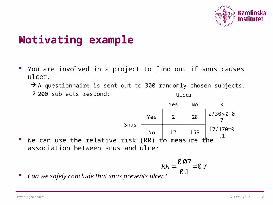
You are involved in a project to find out if snus causes ulcer. A questionnaire is sent out to 300 randomly chosen subjects. 200 subjects respond:

We can use the relative risk (RR) to measure the association between snus and ulcer:

Can we safely conclude that snus prevents ulcer?

Ulcer

Yes No R

Snus

Yes 2 28 2/300.07

No 17 15317/170=0.

1

RR 0.07

0.10.7


Outline

Systematic errors Selection bias Confounding Randomization Reverse causation

Random errors Confidence interval P-value Hypothesis test Significance level Power


One possible explanation

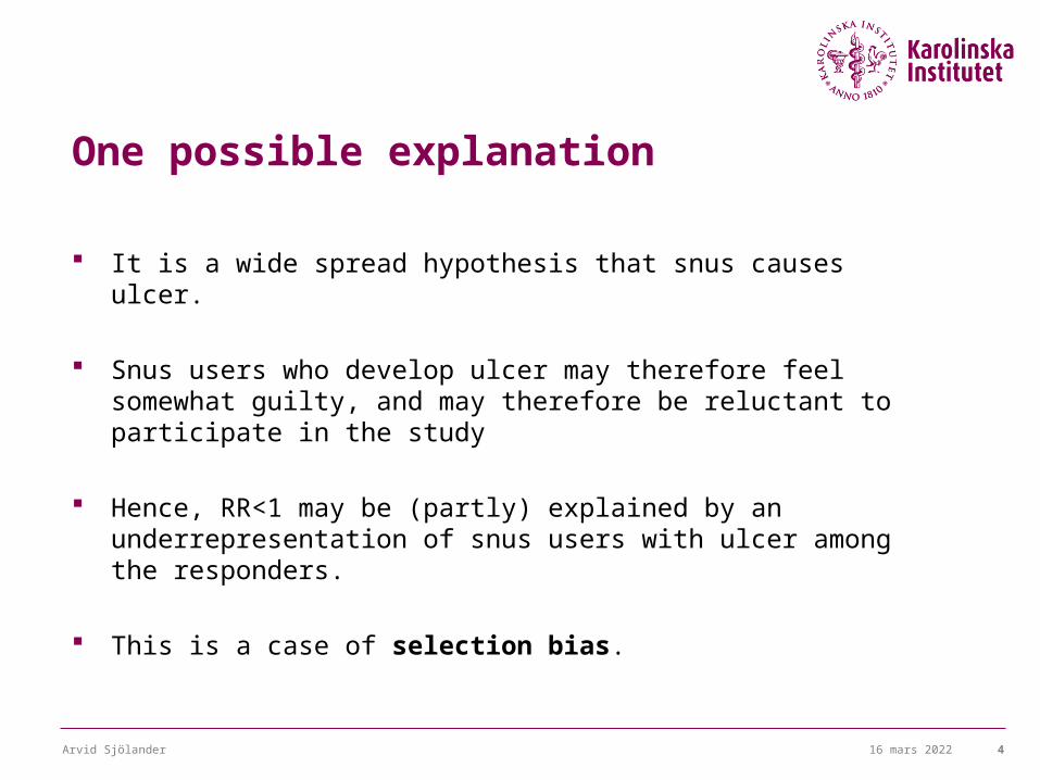
It is a wide spread hypothesis that snus causes ulcer.

Snus users who develop ulcer may therefore feel somewhat guilty, and may therefore be reluctant to participate in the study

Hence, RR<1 may be (partly) explained by an underrepresentation of snus users with ulcer among the responders.

This is a case of selection bias.


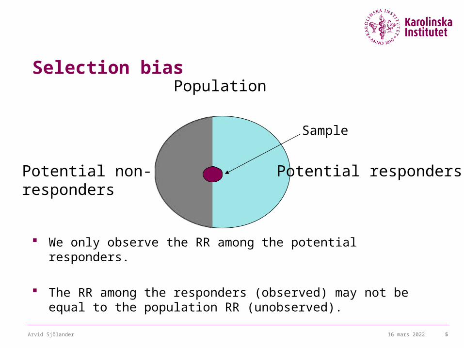
Selection bias

We only observe the RR among the potential responders.

The RR among the responders (observed) may not be equal to the population RR (unobserved).

Population

Potential non-responders

Potential responders

Sample


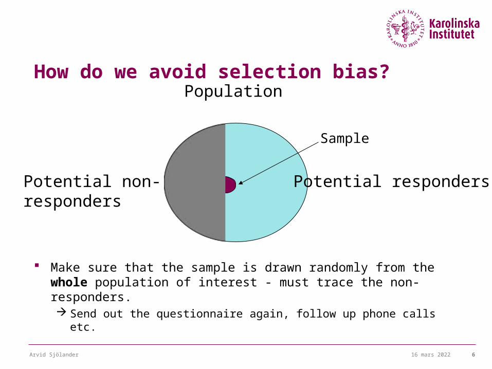
How do we avoid selection bias?

Make sure that the sample is drawn randomly from the whole population of interest - must trace the non-responders. Send out the questionnaire again, follow up phone calls etc.

Population

Potential non-responders

Potential responders

Sample


Another possible explanation

Because of age-trends, young people use snus more often than old people.

For biological reasons, young people have a smaller risks for ulcer than old people.

Hence, RR<1 may be (partly) explained by snus-users being in “better shape” than non-users.

This is a case of confounding, and age is called a confounder.


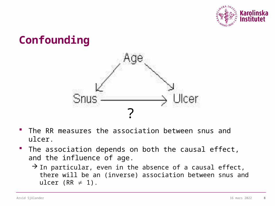
Confounding

The RR measures the association between snus and ulcer. The association depends on both the causal effect, and the

influence of age. In particular, even in the absence of a causal effect, there will be an

(inverse) association between snus and ulcer (RR 1).

?


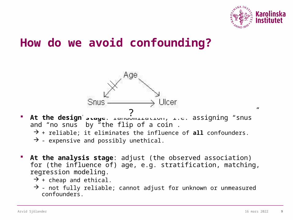
How do we avoid confounding?

At the design stage: randomization, i.e. assigning “snus” and “no snus” by “the flip of a coin”. + reliable; it eliminates the influence of all confounders. - expensive and possibly unethical.

At the analysis stage: adjust (the observed association) for (the influence of) age, e.g. stratification, matching, regression modeling. + cheap and ethical. - not fully reliable; cannot adjust for unknown or unmeasured confounders.

?


Yet another explanation

It is a wide spread hypothesis among physicians that snus causes and aggravates ulcer.

Snus users who suffers from ulcer may therefore be advised by their physicians to quit.

Hence, RR<1 may be (partly) explained by a tendency among people with ulcer to quit using snus.

This is a case of reverse causation.


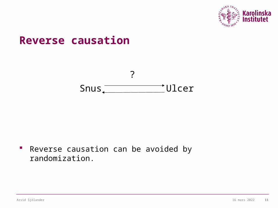
Reverse causation

Reverse causation can be avoided by randomization.

Snus Ulcer

?


Systematic errors

Selection bias, confounding, and reverse causation, are referred to as systematic errors, or bias. “You don’t measure what you are interested in”.

How can you tell if your study is biased? You can’t! (At least not from the observed data).

It is important to design the study carefully and “think ahead” to avoid bias. What may the reason be for potential response/non-response? How can we trace the non-responders? Which are the possible confounders? Do we need to randomize the study? Would randomization be ethical and

practically possible?


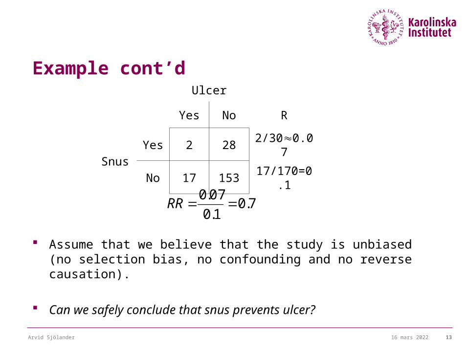
Example cont’d

Assume that we believe that the study is unbiased (no selection bias, no confounding and no reverse causation).

Can we safely conclude that snus prevents ulcer?

Ulcer

Yes No R

SnusYes 2 28 2/300.07

No 17 153 17/170=0.1

RR 0.07

0.10.7


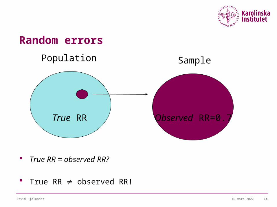
Random errors

True RR = observed RR?

True RR observed RR!

Population Sample

True RR Observed RR=0.7


Confidence interval

Where can we expect the true RR to be?

The 95% Confidence Interval (CI) answers this question. It is a range of plausible values for the true RR. Example: RR=0.7, 95% CI: (0.5,0.9).

The narrower CI, the less uncertainty in the true RR.

The width of the CI depends on the sample size, the larger sample, the narrower CI.

How do we compute a CI? Ask a statistician!

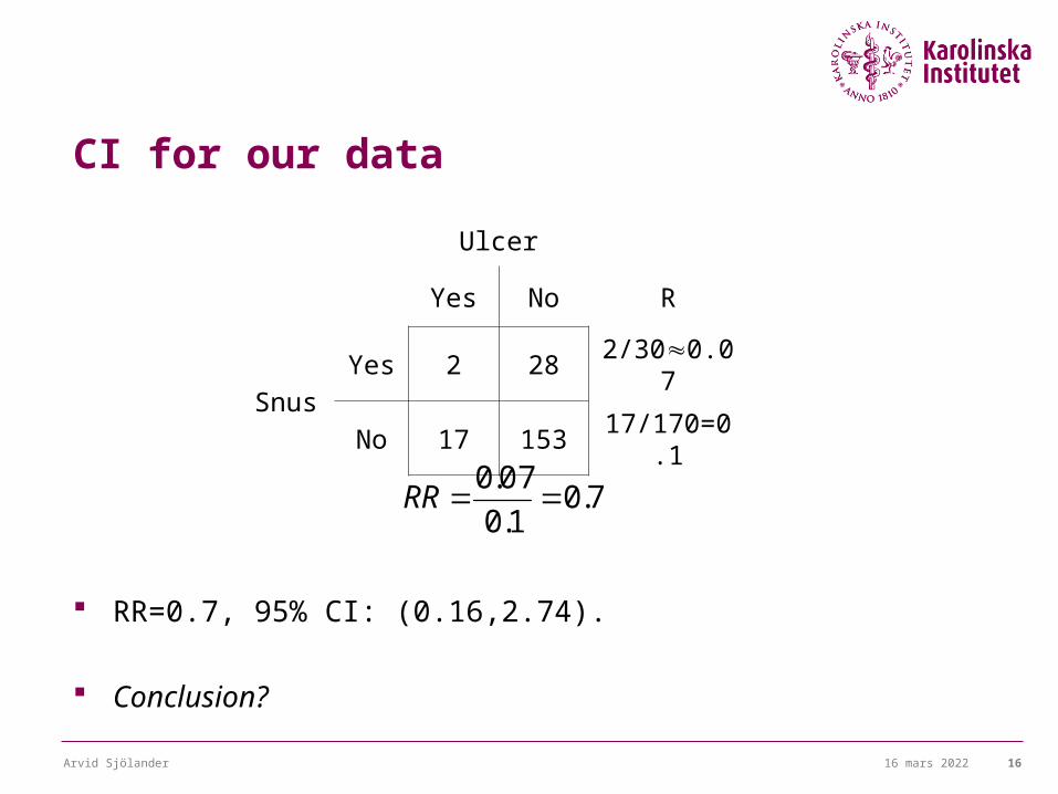
CI for our data

RR=0.7, 95% CI: (0.16,2.74).

Conclusion?


Ulcer

Yes No R

SnusYes 2 28 2/300.07

No 17 153 17/170=0.1

RR 0.07

0.10.7


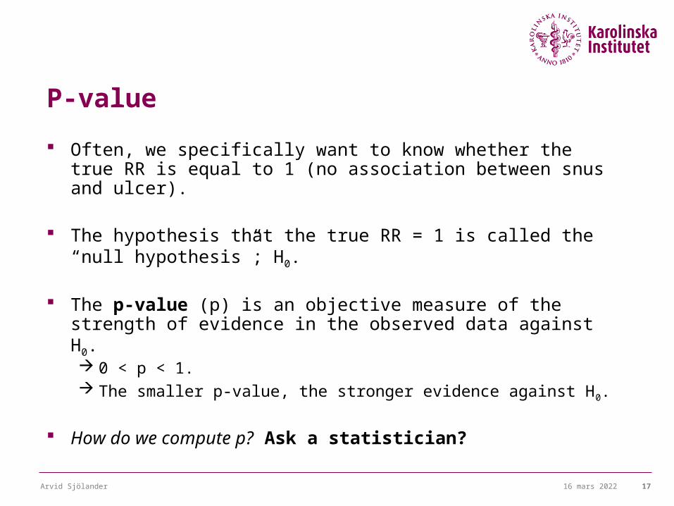
P-value

Often, we specifically want to know whether the true RR is equal to 1 (no association between snus and ulcer).

The hypothesis that the true RR = 1 is called the “null hypothesis”; H0.

The p-value (p) is an objective measure of the strength of evidence in the observed data against H0. 0 < p < 1. The smaller p-value, the stronger evidence against H0.

How do we compute p? Ask a statistician?

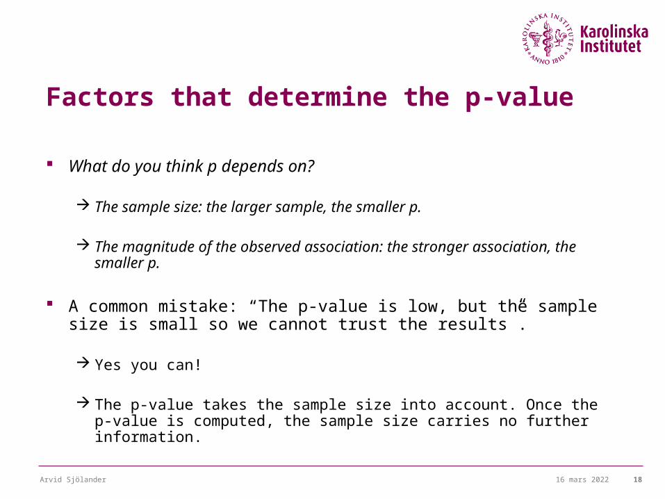
Factors that determine the p-value

What do you think p depends on?

The sample size: the larger sample, the smaller p.

The magnitude of the observed association: the stronger association, the smaller p.

A common mistake: “The p-value is low, but the sample size is small so we cannot trust the results”.

Yes you can!

The p-value takes the sample size into account. Once the p-value is computed, the sample size carries no further information.


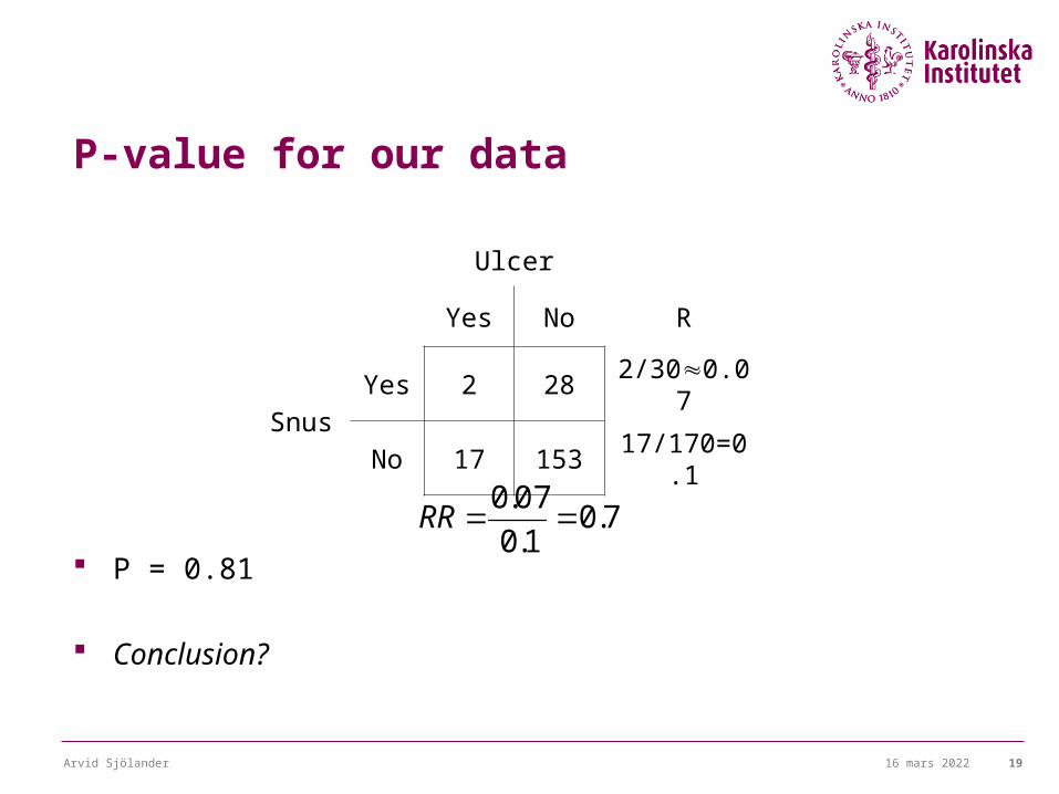
P-value for our data

P = 0.81

Conclusion?


Ulcer

Yes No R

SnusYes 2 28 2/300.07

No 17 153 17/170=0.1

RR 0.07

0.10.7

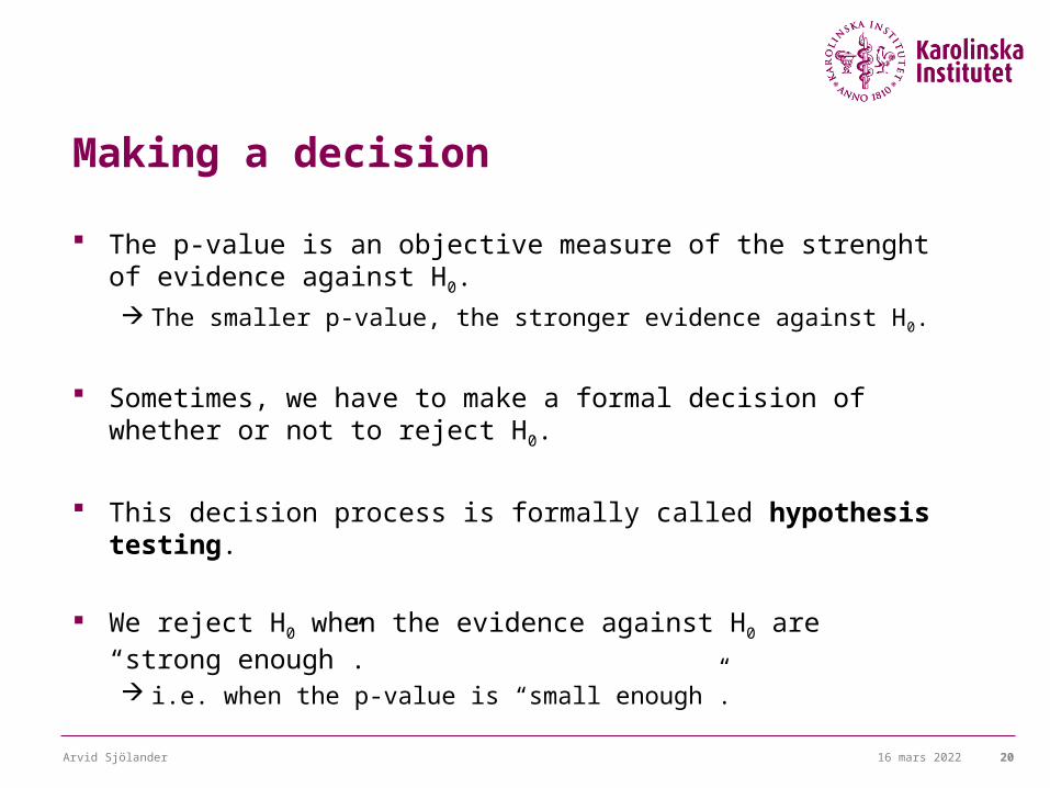
Making a decision

The p-value is an objective measure of the strenght of evidence against H0.

The smaller p-value, the stronger evidence against H0.

Sometimes, we have to make a formal decision of whether or not to reject H0.

This decision process is formally called hypothesis testing.

We reject H0 when the evidence against H0 are “strong enough”. i.e. when the p-value is “small enough”.


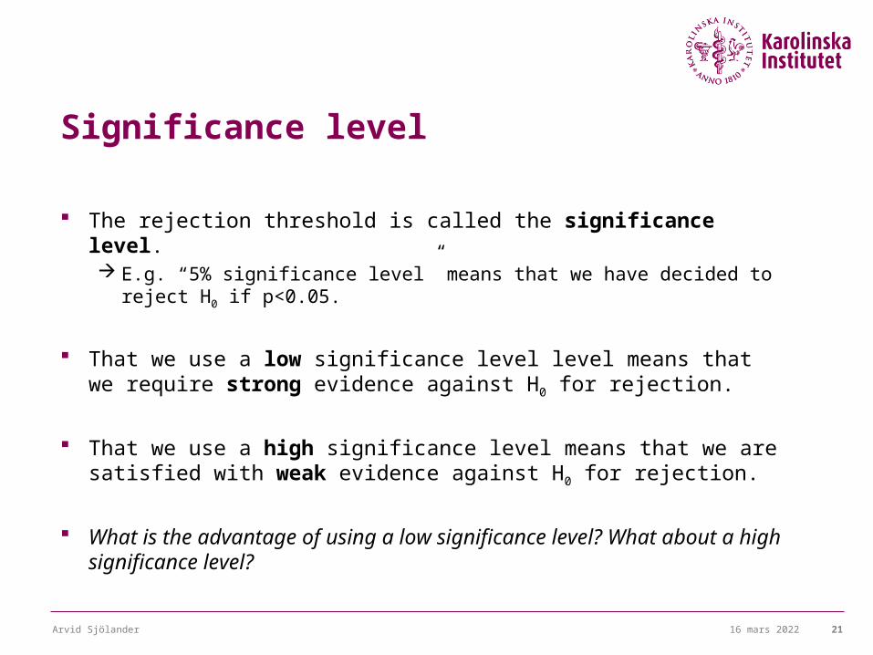
Significance level

The rejection threshold is called the significance level. E.g. “5% significance level” means that we have decided to reject

H0 if p<0.05.

That we use a low significance level level means that we require strong evidence against H0 for rejection.

That we use a high significance level means that we are satisfied with weak evidence against H0 for rejection.

What is the advantage of using a low significance level? What about a high significance level?


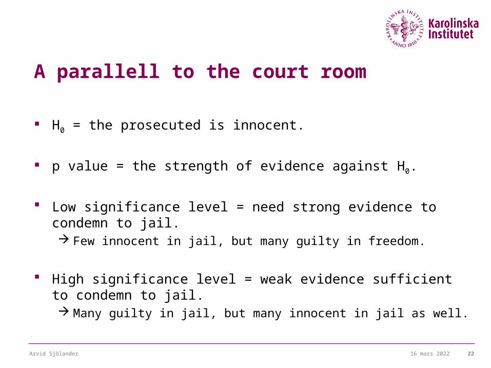
A parallell to the court room

H0 = the prosecuted is innocent.

p value = the strength of evidence against H0.

Low significance level = need strong evidence to condemn to jail. Few innocent in jail, but many guilty in freedom.

High significance level = weak evidence sufficient to condemn to jail. Many guilty in jail, but many innocent in jail as well.


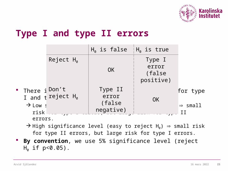
Type I and type II errors

There is always a trade-off between the risk for type I and the risk for type II errors. Low significance level (difficult to reject H0) small risk for type I

errors, but large risk for type II errors. High significance level (easy to reject H0) small risk for type II

errors, but large risk for type I errors.

By convention, we use 5% significance level (reject H0 if p<0.05).


H0 is false H0 is true

Reject H0 OKType I error

(false positive)

Don’t reject H0 Type II error (false negative)

OK

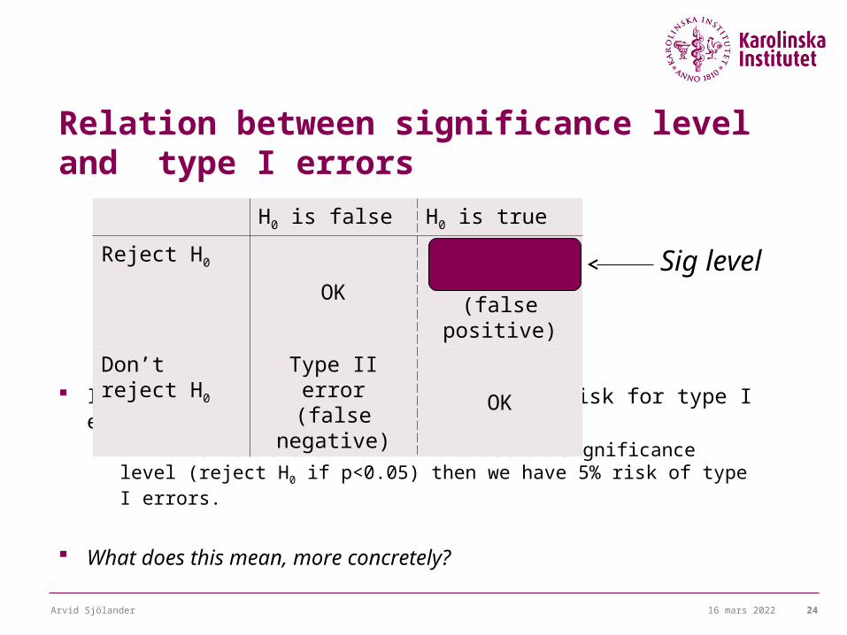
Relation between significance level and type I errors

In fact, the significance level = the risk for type I errors. If we follow the convention and use 5% significance level (reject H0

if p<0.05) then we have 5% risk of type I errors.

What does this mean, more concretely?




(false positive)


OK

Sig level

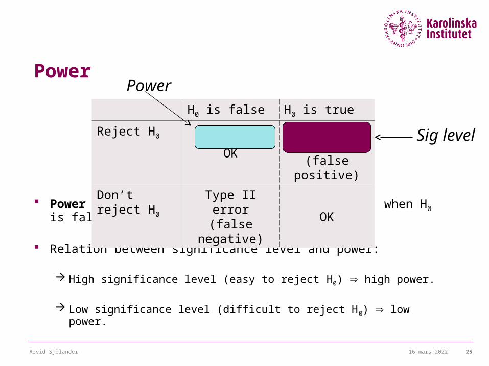
Power

Power = the chance of being able to reject H0, when H0 is false.

Relation between significance level and power:

High significance level (easy to reject H0) high power.

Low significance level (difficult to reject H0) low power.




(false positive)


OK

Sig level

Power

Power calculations

It is important to determine the power of the study before data is collected.

That the power is low means that we will probably not find what we are looking for.

Direct calculation of the power is beyond the scope of this course

Ask a statistician!


Power calculations, cont’d

Heuristically, the power of the study is determined by three factors: The significance level; higher significance level gives higher power. The true RR; stronger association gives higher power. The sample size; larger sample gives higher power.

Typically, we want to have a power of at least 80%. In practice, the significance level is fixed at 5%. We also typically have an idea of what deviations from H0 that are

scientifically relevant to detect (e.g. RR > 1.5). We determine the sample size that we need, to have the desired

power.



Systematic vs random errors

There are two qualitative differences between systematic and random errors.

#1 Data can tell us if an observed association is possibly due to

random errors - check the p-value. Data can never tell us if an observed association is due to

systematic errors. #2

Uncertainty due to random errors can be reduced by increasing the sample size narrower confidence intervals.

Systematic errors results from a poor study design, and can not be reduced by increasing the sample size.


Summary

In medical research, we are often interested in the causal effect of one variable on another.

An observed association between two variables does not necessarily imply that one causes the other.

Always be aware of the following pitfalls: Selection bias Confounding Reverse causation Random errors