1
Project Report on
Transition probabilities in quantum dot with laser pulse using
Runga Kutta method
Submitted For Phd Course Work
By
Manoj Kumar
Under the Supervision of
Prof. Man Mohan
Submitted to
Dr. Poonam Mehta
Department of Physics & Astrophysics
University of Delhi, Delhi
2
Contents
Page
1 - Abstract 3
2 – Introduction 4
3 - Runga Kutta Methods 5
4 - Laser Pulse effect on Quantum Dot 11
5 - Fortran program for transition probabilities in Quantum Dot 13
6 – Results and Discussion 17
7 – References 20

3
Abstract
Here forth order Runga Kutta method is formulated with its physical interpretation.
Further this method is extended to solve the n coupled equation. A program in
FORTRAN to solve coupled equation using Runga Kutta Methods is shown. As
the application of this numerical method, I have considered the laser pulse
interaction with parabolic quantum dot. Time dependent Schrodinger equation is
used to solve this combination and getting some coupled equation in the form
transition probabilities, which are solved here using the FORTRAN programming
and Runge kutta methods.

4
Introduction
The impressive progress in the fabrication of low-dimensional semiconductor
structures during the last two decades has made it possible to reduce the effective device
dimension from three-dimensional bulk materials, to quasi-two dimensional quantum well
systems, to quasi-one dimensional quantum wires, and even to quasi-zero dimensional quantum
dots. The modified electronic and optical properties of these quantum-confined structures, which
are controllable to a certain degree through the flexibility in the structure design, have attracted
considerable attention, and have made them very promising candidates for possible device
applications in semiconductor lasers, microelectronics, non-linear optics, and many other fields.
Quantum dots are small conductive regions in a semiconductor, containing a variable number of
charge carriers (from one to a thousand), that occupy well-defined, discrete quantum states, for
which they are often referred to as artificial atoms. There are several existing devices utilizing
quantum effects in solids, such as semiconductor resonant tunneling diodes (based on
quantum mechanical confinement), superconducting Josephson junction circuits (based on
macroscopic phase coherence), metallic single electron transistors (based on quantization of
charge), molecular electronic devices (based on the inter-dot coupling in a double quantum dot
structure. In this report, i am going to focus on quantum dot which may be called as artificial
atom [1].When a semiconductor sturucture is confined in all direction, their density of states
becomes discrete like atoms as shown in fig 1.
Fig 1. Comparison of the quantization of density of states: (a) bulk, (b) quantum well, (c) quantum wire, (d)
quantum dot. The conduction and valence bands split into overlapping subbands, that get successively narrower as
the electron motion is restricted in more dimensions.
The peculiar quantum behavior of electrons in quantum dots is under investigation in
many laboratories around the world. The tunable size, shape and electron number, as well as the
enhanced electron correlation and magnetic field effects, makes quantum dots excellent objects
for studying fascinating many-electron quantum physics in a controlled way. I am here to study
the pulsed laser effects on quantum dot to find the optical transitions.
A laser can be described as an optical source that emits a coherent beam of photons at an
exact wavelength or frequencies. With the recent progress in ultrafast optics, it is now possible to
5
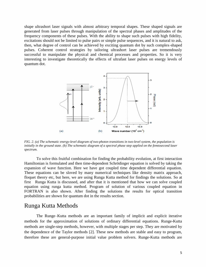
shape ultrashort laser signals with almost arbitrary temporal shapes. These shaped signals are
generated from laser pulses through manipulation of the spectral phases and amplitudes of the
frequency components of these pulses. With the ability to shape such pulses with high fidelity,
excitations should not be limited to pulse pairs or simple pulse sequences, and it is natural to ask,
then, what degree of control can be achieved by exciting quantum dot by such complex-shaped
pulses. Coherent control strategies by tailoring ultrashort laser pulses are tremendously
successful to manipulate the physical and chemical processes and properties. So it is very
interesting to investigate theoretically the effects of ultrafast laser pulses on energy levels of
quantum dot.
FIG. 2. (a) The schematic energy-level diagram of two-photon transitions in two-level system, the population is
initially in the ground state. (b) The schematic diagram of a spectral phase step applied on the femtosecond laser
spectrum.
To solve this fruitful combination for finding the probability evolution, at first interaction
Hamiltonian is formulated and then time-dependent Schrödinger equation is solved by taking the
expansion of wave function. Here we have got coupled time dependent differential equation.
These equations can be sloved by many numerical techniques like density matrix approach,
floquet theory etc, but here, we are using Runga Kutta method for findings the solutions. So at
first Runga Kutta is discussed, and after that it is mentioned that how we can solve coupled
equation using runga kutta method. Program of solution of various coupled equation in
FORTRAN is also shown. After finding the solutions the results for optical transition
probabilities are shown for quantum dot in the results section.
Runga Kutta Methods
The Runge–Kutta methods are an important family of implicit and explicit iterative
methods for the approximation of solutions of ordinary differential equations. Runge-Kutta
methods are single-step methods, however, with multiple stages per step. They are motivated by
the dependence of the Taylor methods [2]. These new methods are stable and easy to program,
therefore these are general-purpose initial value problem solvers. Runge-Kutta methods are

6
among the most popular ODE solvers. They were first studied by Carle Runge and Martin Kutta
around 1900. Modern developments are mostly due to John Butcher in the 1960s.The Runge-
Kutta 2nd order method is as follows:
For equation, , ,dy
f x ydx
00y y
with intial condition, then solution is written as
hkkyy ii
211
2
1
2
1
where
ii yxfk ,1
hkyhxfk ii 12 ,
Only first order ordinary differential equations can be solved by using the Runge-Kutta 2nd order
method. In next sections, it is shown that how Runge-Kutta methods are used to solve higher
order ordinary differential equations or coupled (simultaneous) differential equations.
Runge-Kutta 4th order method.
Runge-Kutta 4th
order method is a numerical technique used to solve ordinary differential
equation of the form
00,, yyyxfdx
dy
So only first order ordinary differential equations can be solved by using the Runge-Kutta 4th
order method. 4th
order means that in this method at every point four times the functions is used
The Runge-Kutta 4th
order method is based on the following
hkakakakayy ii 443322111 (1)
where knowing the value of iyy at ix , we can find the value of 1 iyy at 1ix , and
ii xxh 1
Equation (1) is equated to the first five terms of Taylor series
41,4
4
3
1,3
32
1,2
2
1,1
!4
1
!3
1
!2
1
iiyx
iiyxiiyxiiyxii
xxdx
yd
xxdx
ydxx
dx
ydxx
dx
dyyy
ii
iiiiii
(2)
Knowing that yxfdx
dy, and hxx ii 1
4'''3''2'
1 ,!4
1,
!3
1,
!2
1, hyxfhyxfhyxfhyxfyy iiiiiiiiii (3)
Based on solution of above equation peculiar results are:
7
hkkkkyy ii 43211 226
1 (4)
ii yxfk ,1 (5a)
hkyhxfk ii 12
2
1,
2
1
(5b)
hkyhxfk ii 23
2
1,
2
1 (5c)
hkyhxfk ii 34 , (5d)
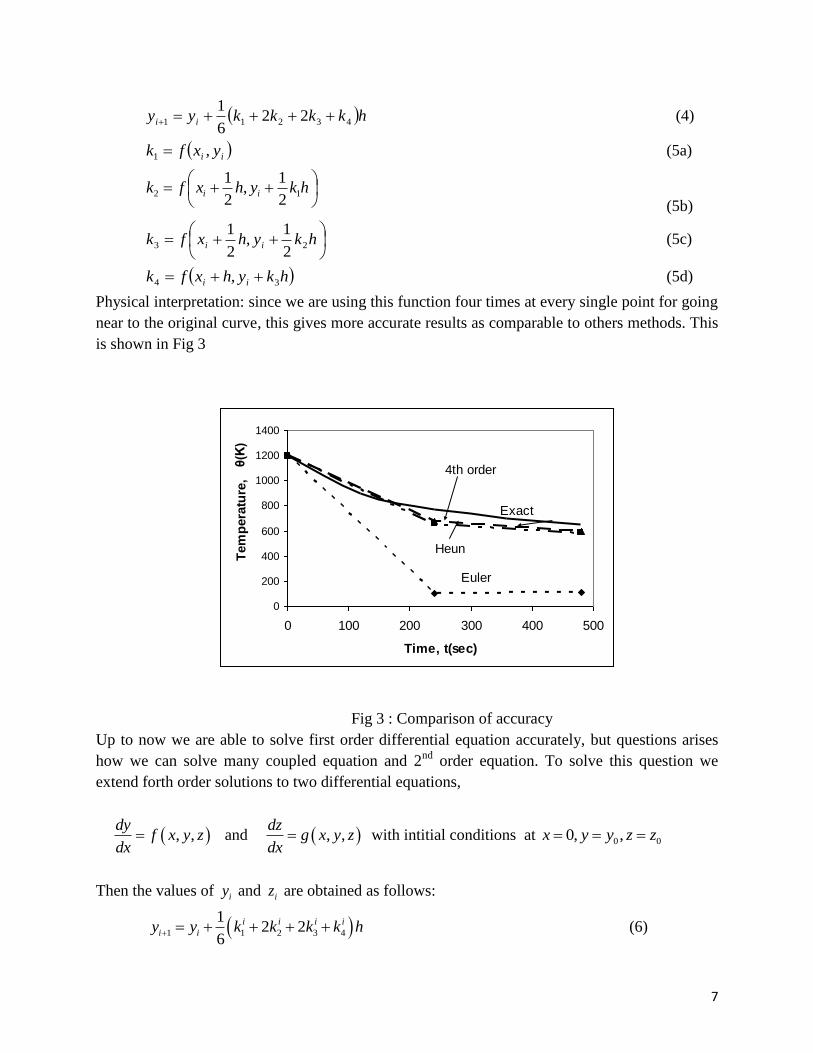
Physical interpretation: since we are using this function four times at every single point for going
near to the original curve, this gives more accurate results as comparable to others methods. This
is shown in Fig 3
Fig 3 : Comparison of accuracy
Up to now we are able to solve first order differential equation accurately, but questions arises
how we can solve many coupled equation and 2nd
order equation. To solve this question we
extend forth order solutions to two differential equations,
, ,dy
f x y zdx
and , ,dz
g x y zdx
with intitial conditions at 0 00, ,x y y z z
Then the values of iy and iz are obtained as follows:
1 1 2 3 4
12 2
6
i i i i
i iy y k k k k h (6)
0
200
400
600
800
1000
1200
1400
0 100 200 300 400 500
Time, t(sec)
Tem
pera
ture
,θ(K)
Exact
4th order
Heun
Euler

8
and 1 1 2 3 4
12 2
6
i i i i
i iz z l l l l h (7)
where
1
1
, ,
, ,
i
i i i
i
i i i
k f x y z
l g x y z
1 12
1 12
2 23
2 23
4 3 3
4 3 3
, ,2 2 2
, ,2 2 2
, ,2 2 2
, ,2 2 2
, ,
, ,
i ii
i i i
i ii
i i i
i ii
i i i
i ii
i i i
i i i
i i i
i i i
i i i
k lhk f x y z
k lhl g x y z
k lhk f x y z
k lhl g x y z
k f x h y k z l
l g x h y k z l
(8)
In the same way we can formulate the solution of n equation , consider n equations are :
1
2
3
, , ,......., ,
, , ,......., ,
, , ,.......,
....................................
....................................
dxf x y z t
dt
dyf x y z t
dt
dzf x y z t
dt
(9)
with intial some intial conditions at 0 0 0 0, , , ..........t t x x y y z z , then the solution of above
equation can be written as
1 1 2 3 4
1 1 2 3 4
1 1 2 3 4
12 2
6
12 2
6
12 2
6
.......................................................
.......................................................
i i i i
i i
i i i i
i i
i i i i
i i
x x k k k k h
y y l l l l h
z z m m m m h
(10)
9
Where
1 1
1 2
1 3
, , ,........,
, , ,..........
, , ,..........
........................................
........................................
i
i i i
i
i i i
i
i i i
k f x y z t
l f x y z t
m f x y z t
1 1 12 1
1 1 12 2
1 1 12 3
, , ,.........,2 2 2 2
, , ,.........,2 2 2 2
, , ,.........,2 2 2 2
...............................................
i i ii
i i i i
i i ii
i i i i
i i ii
i i i i
k l m hk f x y z t
k l m hl f x y z t
k l m hm f x y z t
.........................
........................................................................
(11)
2 2 23 1
2 2 23 2
2 2 23 3
, , ,.........,2 2 2 2
, , ,.........,2 2 2 2
, , ,.........,2 2 2 2
...............................................
i i ii
i i i i
i i ii
i i i i
i i ii
i i i i
k l m hk f x y z t
k l m hl f x y z t
k l m hm f x y z t
.........................
........................................................................
4 1 3 3 3
4 2 3 3 3
4 3 3 3 3
, , ,.........,
, , ,.........,
, , ,.........,
........................................................................
.....
i i i i
i i i i
i i i i
i i i i
i i i i
i i i i
k f x k y l z m t h
l f x k y l z m t h
m f x k y l z m t h
...................................................................
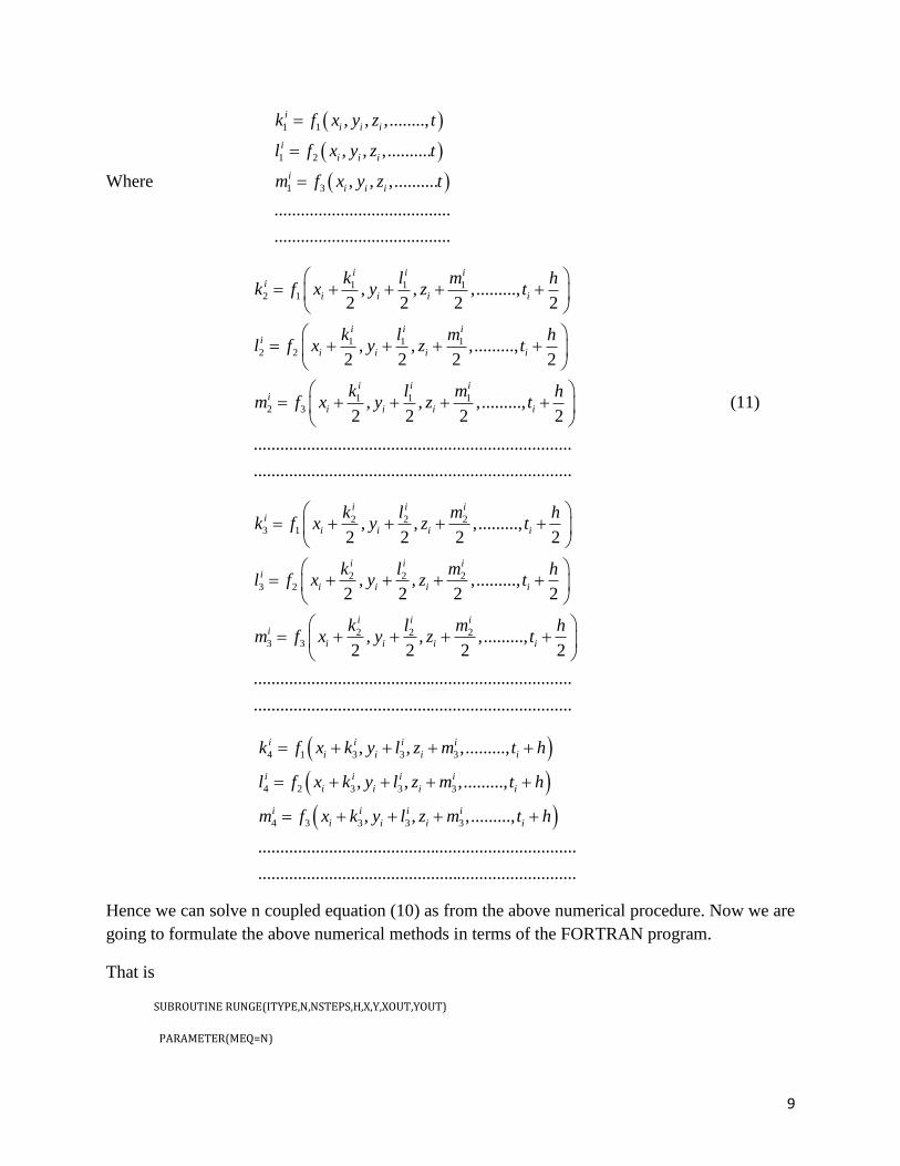
Hence we can solve n coupled equation (10) as from the above numerical procedure. Now we are
going to formulate the above numerical methods in terms of the FORTRAN program.
That is
SUBROUTINE RUNGE(ITYPE,N,NSTEPS,H,X,Y,XOUT,YOUT)
PARAMETER(MEQ=N)
10
REAL Y(MEQ)
REAL Y0(MEQ)
REAL K0(MEQ)
REAL K1(MEQ)
REAL K2(MEQ)
REAL K3(MEQ)
DO 40 J=0,NSTEPS
CALL FUNC(K0,Y,X)
DO 42 I=1,N
Y0(I)=Y(I)
42 Y(I)=Y0(I)+K0(I)*0.5*H
X=X+H*0.5
CALL FUNC(K1,Y,X)
DO 43 I=1,N
43 Y(I)=Y0(I)+K1(I)*0.5*H
CALL FUNC(K2,Y,X)
DO 44 I=1,N
44 Y(I)=Y0(I)+K2(I)*H
X=X+0.5*H
CALL FUNC(K3,Y,X)
DO 45 I=1,N
45 Y(I)=Y0(I)+(K0(I)+2.0*(K1(I)+K2(I))+K3(I))/6.0*H
C1=Y(1)**2+Y(2)**2
C2=Y(3)**2+Y(4)**2
ct=C1+C2
WRITE(6,100) X,C1,C2,ct
100 format (6f15.10)
40 CONTINUE
RETURN
END
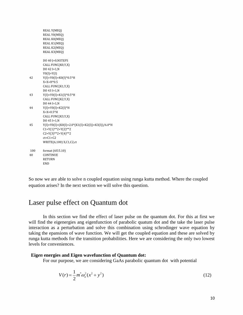
So now we are able to solve n coupled equation using runga kutta method. Where the coupled
equation arises? In the next section we will solve this question.
Laser pulse effect on Quantum dot In this section we find the effect of laser pulse on the quantum dot. For this at first we
will find the eigenergies ang eigenfunction of parabolic quatum dot and the take the laser pulse
interaction as a perturbation and solve this combination using schrodinger wave equation by
taking the epansions of wave function. We will get the coupled equation and these are solved by
runga kutta methods for the transition probabilities. Here we are considering the only two lowest
levels for conveniences.
Eigen energies and Eigen wavefunction of Quantum dot:
For our purpose, we are considering GaAs parabolic quantum dot with potential
* 2 2 21
( ) ( )2
oV r m x y (12)
11
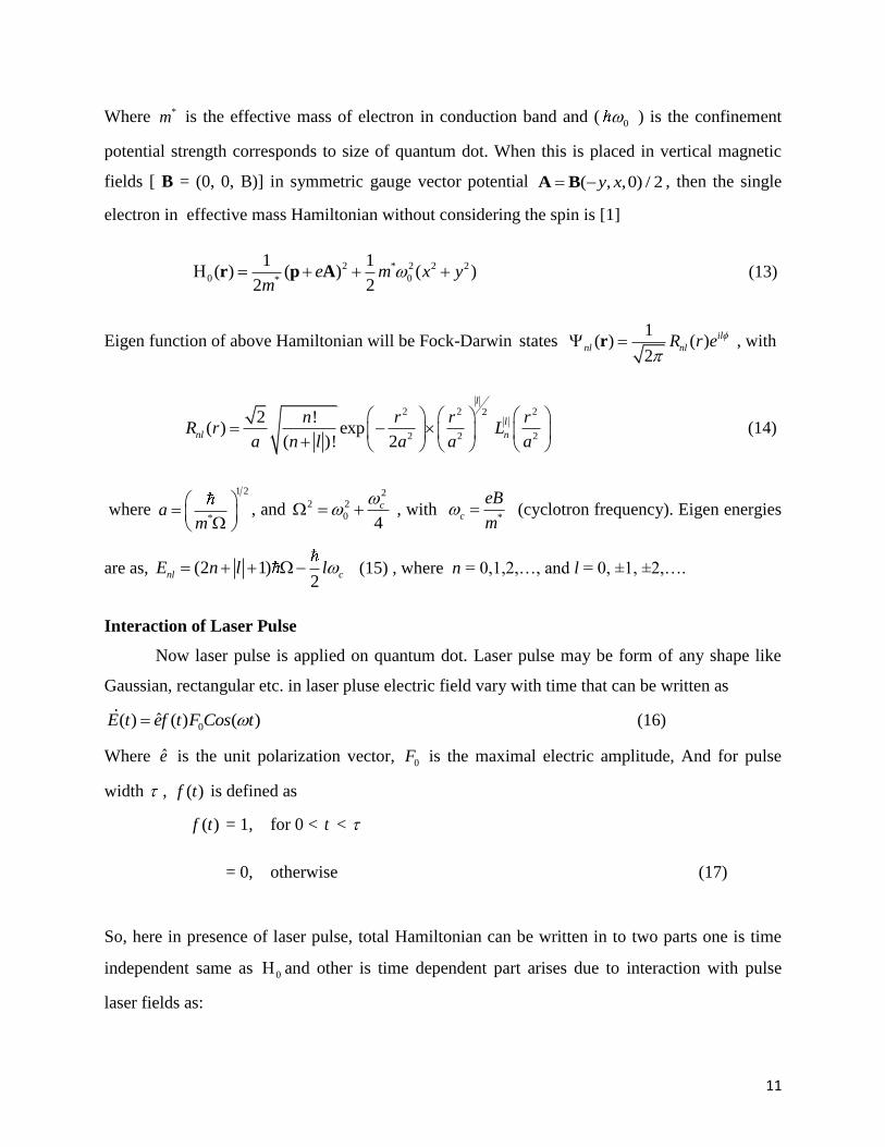
Where *m is the effective mass of electron in conduction band and (0 ) is the confinement
potential strength corresponds to size of quantum dot. When this is placed in vertical magnetic
fields [ B = (0, 0, B)] in symmetric gauge vector potential ( , ,0) / 2y x A B , then the single
electron in effective mass Hamiltonian without considering the spin is [1]
2 * 2 2 2
0 0*
1 1( ) ( ) ( )
2 2e m x y
m r p A (13)
Eigen function of above Hamiltonian will be Fock-Darwin states
1( ) ( )
2
il
nl nlR r e
r , with
2 2 22
2 2 2
2 !( ) exp
( )! 2
l
l
nl n
n r r rR r L
a n l a a a
(14)
where
1 2
*a
m
, and
22 2
04
c , with *c
eB
m (cyclotron frequency). Eigen energies
are as, (2 1)2
nl cE n l l (15) , where n = 0,1,2,…, and l = 0, ±1, ±2,….
Interaction of Laser Pulse
Now laser pulse is applied on quantum dot. Laser pulse may be form of any shape like
Gaussian, rectangular etc. in laser pluse electric field vary with time that can be written as
0ˆ( ) ( ) ( )E t ef t F Cos t (16)
Where e is the unit polarization vector, 0F is the maximal electric amplitude, And for pulse
width , ( )f t is defined as
( )f t = 1, for 0 < t <
= 0, otherwise (17)
So, here in presence of laser pulse, total Hamiltonian can be written in to two parts one is time
independent same as 0 and other is time dependent part arises due to interaction with pulse
laser fields as:
12
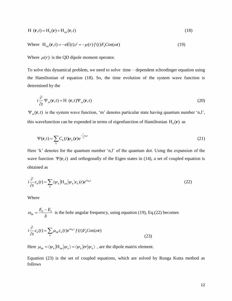
0 int( , ) ( ) ( , )t t r r r (18)
Where int 0( , ) ( ). ( ) ( ) ( )t eE t r r f t F Cos t r (19)
Where ( )r is the QD dipole moment operator.
To solve this dynamical problem, we need to solve time – dependent schrodinger equation using
the Hamiltonian of equation (18). So, the time evolution of the system wave function is
determined by the
( , ) ( , ) ( , )m mi t t tt
r r r (20)
( , )m t r is the system wave function, ‘m’ denotes particular state having quantum number ‘n,l’,
this wavefunction can be expended in terms of eigenfunction of Hamiltonian 0 ( ) r as
( , ) ( ) ( )k
it
k k
k
t C t e
r r (21)
Here ‘k’ denotes for the quantum number ‘n,l’ of the quantum dot. Using the expansion of the
wave function ( , )t r and orthogonally of the Eigen states in (14), a set of coupled equation is
obtained as
int( ) ( ) bki t
b b k k
k
i c t c t et
(22)
Where
b kbk
E E
is the bohr angular frequency, using equation (19), Eq.(22) becomes
0( ) ( ) ( ) ( )bki t
b bk k
k
i c t c t e f t F Cos tt
(23)
Here intbk b k b ker , are the dipole matrix element.
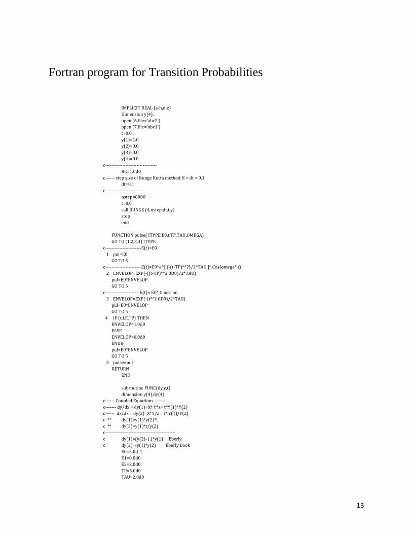
Equation (23) is the set of coupled equations, which are solved by Runga Kutta method as
follows
13
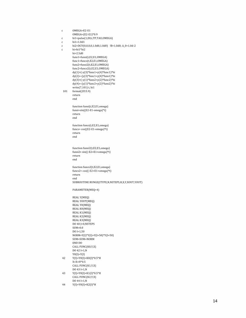
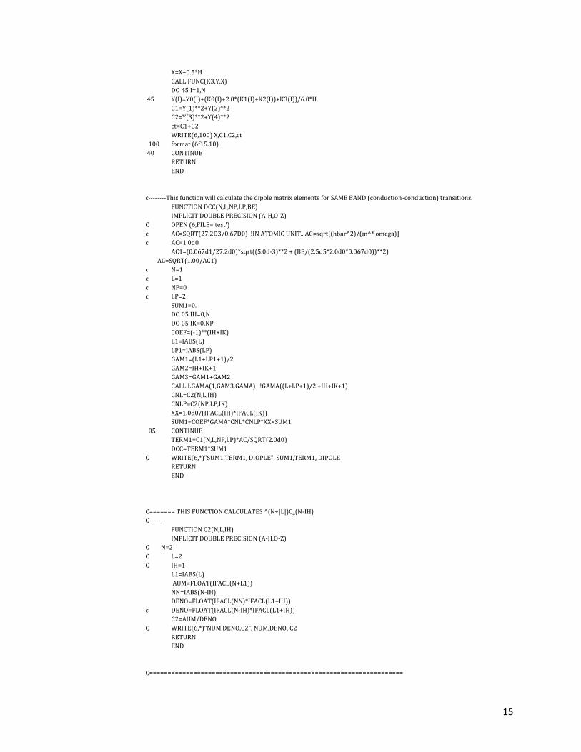
Fortran program for Transition Probabilities
IMPLICIT REAL (a-h,o-z)
Dimension y(4),
open (6,file='abc2')
open (7,file='abc1')
t=0.0
y(1)=1.0
y(2)=0.0
y(3)=0.0
y(4)=0.0
c---------------------------------
BE=1.0d0
c------ step size of Runge Kutta method H = dt = 0.1
dt=0.1
c-------------------------
nstep=8000
t=0.0
call RUNGE (4,nstep,dt,t,y)
stop
end
FUNCTION pulse( ITYPE,E0,t,TP,TAU,OMEGA)
GO TO (1,2,3,4) ITYPE
c-----------------------E(t)=E0
1 pul=E0
GO TO 5
c-----------------------E(t)=E0*e^[ {-(t-TP)**2}/2*TAU ]* Cos(omega* t)
2 ENVELOP=EXP(-((t-TP)**2.0D0)/2*TAU)
pul=E0*ENVELOP
GO TO 5
c----------------------E(t)= E0* Gaussian
3 ENVELOP=EXP(-(t**2.0D0)/2*TAU)
pul=E0*ENVELOP
GO TO 5
4 IF (t.LE.TP) THEN
ENVELOP=1.0d0
ELSE
ENVELOP=0.0d0
ENDIF
pul=E0*ENVELOP
GO TO 5
5 pulse=pul
RETURN
END
subroutine FUNC(dy,y,t)
dimension y(4),dy(4)
c------ Coupled Equations -------
c------- dy/dx = dy(1)=X* Y*z= t*Y(1)*Y(2)
c------ dz/dx = dy(2)=X*Y/z = t* Y(1)/Y(2)
c ** dy(1)=y(1)*y(2)*t
c ** dy(2)=y(1)*t/y(2)
c---------------------------------------------
c dy(1)=(y(2)-1.)*y(1) !Eberly
c dy(2)=-y(1)*y(2) !Eberly Book
E0=5.0d-1
E1=0.0d0
E2=2.0d0
TP=5.0d0
TAU=2.0d0
14
c OMEGA=E2-E1
OMEGA=(E2-E1)*0.9
c hi1=pulse(1,E0,t,TP,TAU,OMEGA)
c hi1=1.0d1
c hi2=DCV(0,0,0,0,1.0d0,1.0d0) !B=1.0d0; A_0=1.0d-2
c hi=hi1*hi2
hi=2.5d0
funs1=funsi(t,E2,E1,OMEGA)
func1=funcs(t,E2,E1,OMEGA)
funs2=funsi2(t,E2,E1,OMEGA)
func2=funcs2(t,E2,E1,OMEGA)
dy(1)=(-y(3)*funs1+y(4)*func1)*hi
dy(2)=-(y(3)*func1+y(4)*funs1)*hi
dy(3)=(-y(1)*funs2+y(2)*func2)*hi
dy(4)=-(y(1)*func2+y(2)*funs2)*hi
write(7,101) t, hi1
101 format(2f15.9)
return
end
function funsi(t,E2,E1,omega)
funsi=sin((E2-E1-omega)*t)
return
end
function funcs(t,E2,E1,omega)
funcs= cos((E2-E1-omega)*t)
return
end
function funsi2(t,E2,E1,omega)
funsi2= sin((-E2+E1+omega)*t)
return
end
function funcs2(t,E2,E1,omega)
funcs2= cos((-E2+E1+omega)*t)
return
end
SUBROUTINE RUNGE(ITYPE,N,NSTEPS,H,X,Y,XOUT,YOUT)
PARAMETER(MEQ=4)
REAL Y(MEQ)
REAL YOUT(MEQ)
REAL Y0(MEQ)
REAL K0(MEQ)
REAL K1(MEQ)
REAL K2(MEQ)
REAL K3(MEQ)
DO 40 J=0,NSTEPS
SUM=0.0
DO I=1,50
NORM=Y(I)*Y(I)+Y(I+50)*Y(I+50)
SUM=SUM+NORM
END DO
CALL FUNC(K0,Y,X)
DO 42 I=1,N
Y0(I)=Y(I)
42 Y(I)=Y0(I)+K0(I)*0.5*H
X=X+H*0.5
CALL FUNC(K1,Y,X)
DO 43 I=1,N
43 Y(I)=Y0(I)+K1(I)*0.5*H
CALL FUNC(K2,Y,X)
DO 44 I=1,N
44 Y(I)=Y0(I)+K2(I)*H
15
X=X+0.5*H
CALL FUNC(K3,Y,X)
DO 45 I=1,N
45 Y(I)=Y0(I)+(K0(I)+2.0*(K1(I)+K2(I))+K3(I))/6.0*H
C1=Y(1)**2+Y(2)**2
C2=Y(3)**2+Y(4)**2
ct=C1+C2
WRITE(6,100) X,C1,C2,ct
100 format (6f15.10)
40 CONTINUE
RETURN
END
c--------This function will calculate the dipole matrix elements for SAME BAND (conduction-conduction) transitions.
FUNCTION DCC(N,L,NP,LP,BE)
IMPLICIT DOUBLE PRECISION (A-H,O-Z)
C OPEN (6,FILE='test')
c AC=SQRT(27.2D3/0.67D0) !IN ATOMIC UNIT.. AC=sqrt[(hbar^2)/(m^* omega)]
c AC=1.0d0
AC1=(0.067d1/27.2d0)*sqrt((5.0d-3)**2 + (BE/(2.5d5*2.0d0*0.067d0))**2)
AC=SQRT(1.00/AC1)
c N=1
c L=1
c NP=0
c LP=2
SUM1=0.
DO 05 IH=0,N
DO 05 IK=0,NP
COEF=(-1)**(IH+IK)
L1=IABS(L)
LP1=IABS(LP)
GAM1=(L1+LP1+1)/2
GAM2=IH+IK+1
GAM3=GAM1+GAM2
CALL LGAMA(1,GAM3,GAMA) !GAMA((L+LP+1)/2 +IH+IK+1)
CNL=C2(N,L,IH)
CNLP=C2(NP,LP,IK)
XX=1.0d0/(IFACL(IH)*IFACL(IK))
SUM1=COEF*GAMA*CNL*CNLP*XX+SUM1
05 CONTINUE
TERM1=C1(N,L,NP,LP)*AC/SQRT(2.0d0)
DCC=TERM1*SUM1
C WRITE(6,*)"SUM1,TERM1, DIOPLE", SUM1,TERM1, DIPOLE
RETURN
END
C======= THIS FUNCTION CALCULATES ^(N+|L|)C_(N-IH)
C-------
FUNCTION C2(N,L,IH)
IMPLICIT DOUBLE PRECISION (A-H,O-Z)
C N=2
C L=2
C IH=1
L1=IABS(L)
AUM=FLOAT(IFACL(N+L1))
NN=IABS(N-IH)
DENO=FLOAT(IFACL(NN)*IFACL(L1+IH))
c DENO=FLOAT(IFACL(N-IH)*IFACL(L1+IH))
C2=AUM/DENO
C WRITE(6,*)"NUM,DENO,C2", NUM,DENO, C2
RETURN
END
C=====================================================================
16
c----------This function will calculate {[(n!)*(np!)]/[(n+l)! *(np+lp)!]}^(1/2)* del_{l,lp}
C=====================================================================
C---------- (N & L) AND (NP & LP) ARE THE PRINCIPLE AND ANGULAR QUANTUM NUMBERS OF THE TWO STATES in different
BANDS.
FUNCTION CV1(N,L,NP,LP)
IMPLICIT DOUBLE PRECISION (A-H,O-Z)
NUM=IFACL(N)*IFACL(NP)
L1=IABS(L)
LP1=IABS(LP)
DENO=IFACL(N+L1)*IFACL(NP+LP1) !(N+L)! * (NP+LP)!
IF (L.EQ.LP) THEN
CV1=SQRT(NUM/DENO)
ELSE
CV1=0 !THE if STATEMENT GIVES THE DELTA FUNCTION.
ENDIF
RETURN
END
C-----------------------------------
c----------This function will calculate {[(n!)*(np!)]/[(n+l)! *(np+lp)!]}^(1/2) *del_{l,lp+-1}
c (N & L) AND (NP & LP) ARE THE PRINCIPLE AND ANGULAR QUANTUM NUMBERS OF THE TWO STATES in the same band...
FUNCTION C1(N,L,NP,LP)
IMPLICIT DOUBLE PRECISION (A-H,O-Z)
NUM=IFACL(N)*IFACL(NP)
L1=IABS(L)
LP1=IABS(LP)
DENO=IFACL(N+L1)*IFACL(NP+LP1) !(N+L)! * (NP+LP)!
IF (L.EQ.(LP+1)) THEN
C1=SQRT(NUM/DENO)
ELSE IF (L.EQ.(LP-1)) THEN
C1=SQRT(NUM/DENO)
ELSE
C1=0 !THE if STATEMENT GIVES THE DELTA FUNCTION.
ENDIF
RETURN
END
C-----------------------------------
c----------THIS FUNCTION CALCULATES THE FACTORIAL OF NN..
FUNCTION IFACL(NN)
INTEGER NN,NN1,IFACL
IFACL=1
DO 11 NN1=1,NN
IFACL=IFACL*NN1
11 CONTINUE
RETURN
END
c---------------------------------
SUBROUTINE GAMMA(X,GA)
C
C ==================================================
C Purpose: Compute the gamma function â(x)
C Input : x --- Argument of â(x)
C ( x is not equal to 0,-1,-2,úúú )
C Output: GA --- â(x)
C ==================================================
C
IMPLICIT DOUBLE PRECISION (A-H,O-Z)
DIMENSION G(26)
PI=3.141592653589793D0
IF (X.EQ.INT(X)) THEN
IF (X.GT.0.0D0) THEN
GA=1.0D0
17
M1=X-1
DO 10 K=2,M1
10 GA=GA*K
ELSE
GA=1.0D+300
ENDIF
ELSE
IF (DABS(X).GT.1.0D0) THEN
Z=DABS(X)
M=INT(Z)
R=1.0D0
DO 15 K=1,M
15 R=R*(Z-K)
Z=Z-M
ELSE
Z=X
ENDIF
DATA G/1.0D0,0.5772156649015329D0,
& -0.6558780715202538D0, -0.420026350340952D-1,
& 0.1665386113822915D0,-.421977345555443D-1,
& -.96219715278770D-2, .72189432466630D-2,
& -.11651675918591D-2, -.2152416741149D-3,
& .1280502823882D-3, -.201348547807D-4,
& -.12504934821D-5, .11330272320D-5,
& -.2056338417D-6, .61160950D-8,
& .50020075D-8, -.11812746D-8,
& .1043427D-9, .77823D-11,
& -.36968D-11, .51D-12,
& -.206D-13, -.54D-14, .14D-14, .1D-15/
GR=G(26)
DO 20 K=25,1,-1
20 GR=GR*Z+G(K)
GA=1.0D0/(GR*Z)
IF (DABS(X).GT.1.0D0) THEN
GA=GA*R
IF (X.LT.0.0D0) GA=-PI/(X*GA*DSIN(PI*X))
ENDIF
ENDIF
RETURN
END
Results and Discussion
Using the above numerical technique, coupled equations are solved, and we get the
transition probabilities of electron between the energy levels of quantum dot causing by laser
pulse, here we are using three different types of laser pulses. So we are getting three different
transition probabilities between the first two levels.

18
Fig 4 : transitition probabitlity between two lowest level are shown for the constant value of laser pulse electric field
magnitude. These oscilation are known as rabi oscilations.
(1) for laser pulse with constant electric fields, the transition probabilities are shown in Fig4, on
x axis the time scale is represented in seconds and on y axis the transition probability is shown.
The upper curve showing the ground state probability and lower state showing first level
transistion probability.
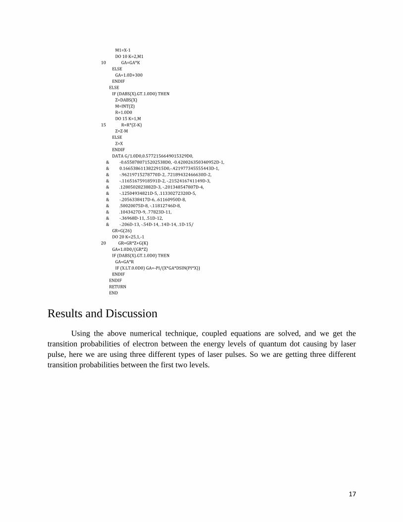
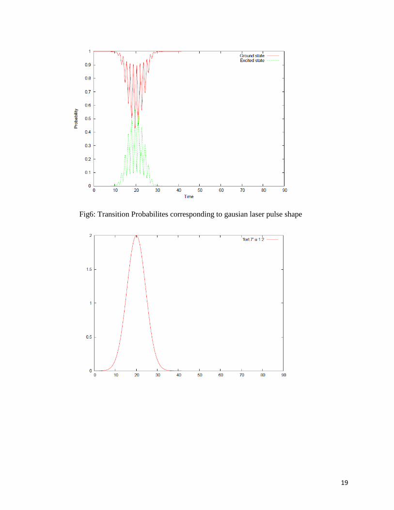
(2) for Gausisan laser pluse ( as shown in Fig5) the transition probabilities are shown in fig6
Fig5: Gaussian pulse shape
19
Fig6: Transition Probabilites corresponding to gausian laser pulse shape
20
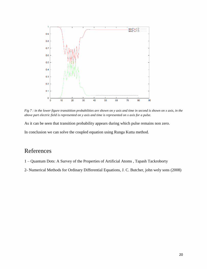
Fig 7 : in the lower figure transitition probabilities are shown on y axis and time in second is shown on x axis, in the
above part electric field is represented on y axis and time is represented on x axis for a pulse.
As it can be seen that transition probability appears during which pulse remains non zero.
In conclusion we can solve the coupled equation using Runga Kutta method.
References
1 – Quantum Dots: A Survey of the Properties of Artificial Atoms , Tapash Tackroborty
2- Numerical Methods for Ordinary Differential Equations, J. C. Butcher, john wely sons (2008)
Recommended