Total Variation
Total Variation in Image Analysis(The Homo Erectus Stage?)
François Lauze
1Department of Computer ScienceUniversity of Copenhagen
Hólar Summer School on Sparse Coding, August 2010
Total Variation
Outline
1 MotivationOrigin and uses of Total VariationDenoisingTikhonov regularization1-D computation on step edges
2 Total Variation IFirst definitionRudin-Osher-FatemiInpainting/Denoising
3 Total Variation IIRelaxing the derivative constraintsDefinition in actionUsing the new definition in denoising: Chambolle algorithmImage Simplification
4 Bibliography
5 The End
Total Variation
Motivation
Origin and uses of Total Variation
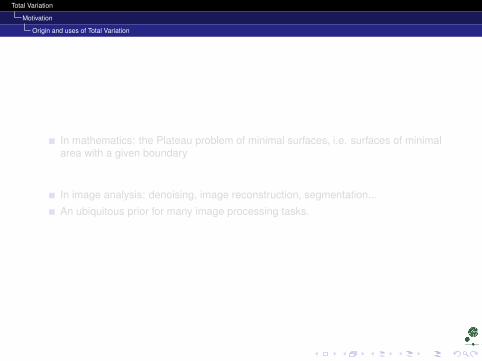
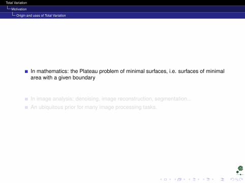
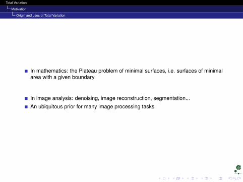
In mathematics: the Plateau problem of minimal surfaces, i.e. surfaces of minimalarea with a given boundary
In image analysis: denoising, image reconstruction, segmentation...
An ubiquitous prior for many image processing tasks.
Total Variation
Motivation
Origin and uses of Total Variation
In mathematics: the Plateau problem of minimal surfaces, i.e. surfaces of minimalarea with a given boundary
In image analysis: denoising, image reconstruction, segmentation...
An ubiquitous prior for many image processing tasks.
Total Variation
Motivation
Origin and uses of Total Variation
In mathematics: the Plateau problem of minimal surfaces, i.e. surfaces of minimalarea with a given boundary
In image analysis: denoising, image reconstruction, segmentation...
An ubiquitous prior for many image processing tasks.
Total Variation
Motivation
Denoising
Outline
1 MotivationOrigin and uses of Total VariationDenoisingTikhonov regularization1-D computation on step edges
2 Total Variation IFirst definitionRudin-Osher-FatemiInpainting/Denoising
3 Total Variation IIRelaxing the derivative constraintsDefinition in actionUsing the new definition in denoising: Chambolle algorithmImage Simplification
4 Bibliography
5 The End
Total Variation
Motivation
Denoising
Denoising
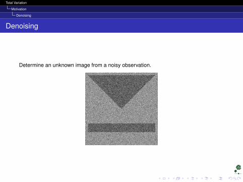
Determine an unknown image from a noisy observation.
Total Variation
Motivation
Denoising
Methods
All methods based on some statistical inference.
Fourier/Wavelets
Markov Random Fields
Variational and Partial Differential Equations methods
...
We focus on variational and PDE methods.
Total Variation
Motivation
Denoising
A simple corruption model
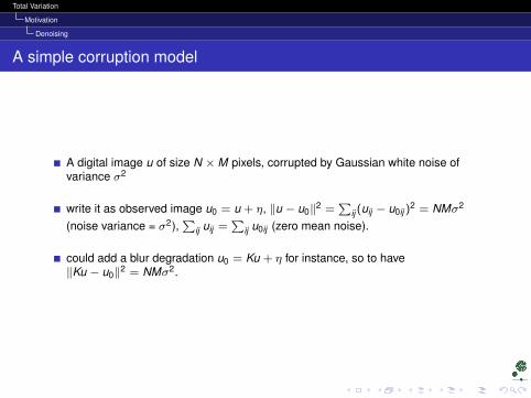
A digital image u of size N ×M pixels, corrupted by Gaussian white noise ofvariance σ2
write it as observed image u0 = u + η, ‖u − u0‖2 =∑
ij (uij − u0ij )2 = NMσ2
(noise variance = σ2),∑
ij uij =∑
ij u0ij (zero mean noise).
could add a blur degradation u0 = Ku + η for instance, so to have‖Ku − u0‖2 = NMσ2.
Total Variation
Motivation
Denoising
A simple corruption model
A digital image u of size N ×M pixels, corrupted by Gaussian white noise ofvariance σ2
write it as observed image u0 = u + η, ‖u − u0‖2 =∑
ij (uij − u0ij )2 = NMσ2
(noise variance = σ2),∑
ij uij =∑
ij u0ij (zero mean noise).
could add a blur degradation u0 = Ku + η for instance, so to have‖Ku − u0‖2 = NMσ2.
Total Variation
Motivation
Denoising
Recovery
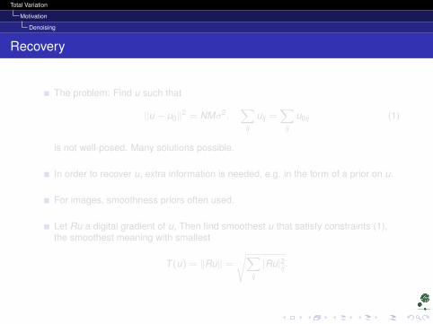
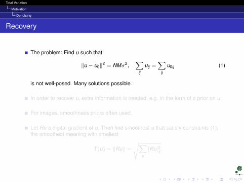
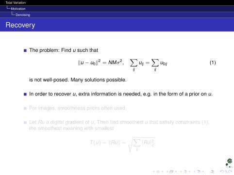
The problem: Find u such that
‖u − u0‖2 = NMσ2,∑
ij
uij =∑
ij
u0ij (1)
is not well-posed. Many solutions possible.
In order to recover u, extra information is needed, e.g. in the form of a prior on u.
For images, smoothness priors often used.
Let Ru a digital gradient of u, Then find smoothest u that satisfy constraints (1),the smoothest meaning with smallest
T (u) = ‖Ru‖ =
√∑ij
|Ru|2ij .
Total Variation
Motivation
Denoising
Recovery
The problem: Find u such that
‖u − u0‖2 = NMσ2,∑
ij
uij =∑
ij
u0ij (1)
is not well-posed. Many solutions possible.
In order to recover u, extra information is needed, e.g. in the form of a prior on u.
For images, smoothness priors often used.
Let Ru a digital gradient of u, Then find smoothest u that satisfy constraints (1),the smoothest meaning with smallest
T (u) = ‖Ru‖ =
√∑ij
|Ru|2ij .
Total Variation
Motivation
Tikhonov regularization
Outline
1 MotivationOrigin and uses of Total VariationDenoisingTikhonov regularization1-D computation on step edges
2 Total Variation IFirst definitionRudin-Osher-FatemiInpainting/Denoising
3 Total Variation IIRelaxing the derivative constraintsDefinition in actionUsing the new definition in denoising: Chambolle algorithmImage Simplification
4 Bibliography
5 The End
Total Variation
Motivation
Tikhonov regularization
Tikhonov regularization
It can be show that this is equivalent to minimize
E(u) = ‖Ku − u0‖2 + λ‖Ru‖2
for a λ = λ(σ) (Wahba?).
E(u) minimizaton can be derived from a Maximum a Posteriori formulation
Arg.maxu
p(u|u0) =p(u0|u)p(u)
p(u0)
Rewriting in a continuous setting:
E(u) =
∫Ω
(Ku − uo)2 dx + λ
∫Ω|∇u|2 dx
Total Variation
Motivation
Tikhonov regularization
How to solve?
Solution satisfies the Euler-Lagrange equation for E :
K∗ (Ku − u0)− λ∆u = 0.
(K∗ is the adjoint of K )
A linear equation, easy to implement, and many fast solvers exit, but...
Total Variation
Motivation
Tikhonov regularization
How to solve?
Solution satisfies the Euler-Lagrange equation for E :
K∗ (Ku − u0)− λ∆u = 0.
(K∗ is the adjoint of K )
A linear equation, easy to implement, and many fast solvers exit, but...
Total Variation
Motivation
Tikhonov regularization
How to solve?
Solution satisfies the Euler-Lagrange equation for E :
K∗ (Ku − u0)− λ∆u = 0.
(K∗ is the adjoint of K )
A linear equation, easy to implement, and many fast solvers exit, but...
Total Variation
Motivation
Tikhonov regularization
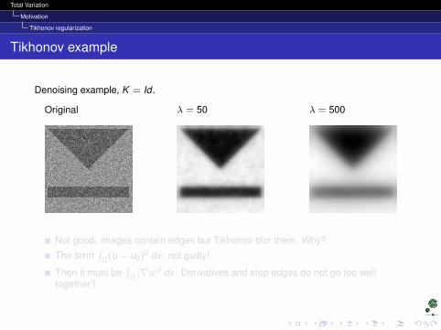
Tikhonov example
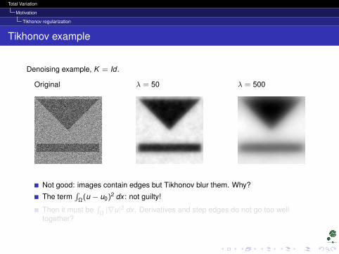
Denoising example, K = Id .
Original λ = 50 λ = 500
Not good: images contain edges but Tikhonov blur them. Why?
The term∫
Ω(u − u0)2 dx : not guilty!
Then it must be∫
Ω |∇u|2 dx . Derivatives and step edges do not go too welltogether?
Total Variation
Motivation
Tikhonov regularization
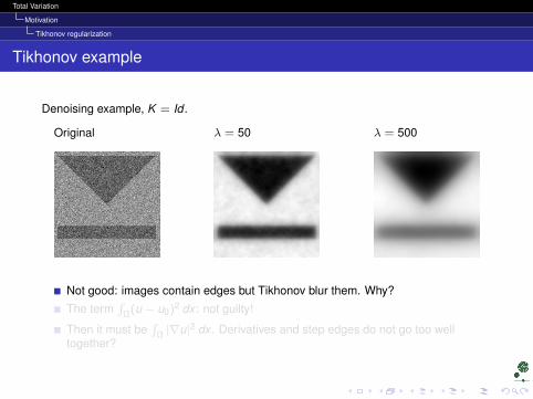
Tikhonov example
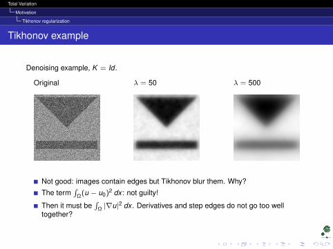
Denoising example, K = Id .
Original λ = 50 λ = 500
Not good: images contain edges but Tikhonov blur them. Why?
The term∫
Ω(u − u0)2 dx : not guilty!
Then it must be∫
Ω |∇u|2 dx . Derivatives and step edges do not go too welltogether?
Total Variation
Motivation
Tikhonov regularization
Tikhonov example
Denoising example, K = Id .
Original λ = 50 λ = 500
Not good: images contain edges but Tikhonov blur them. Why?
The term∫
Ω(u − u0)2 dx : not guilty!
Then it must be∫
Ω |∇u|2 dx . Derivatives and step edges do not go too welltogether?
Total Variation
Motivation
1-D computation on step edges
Outline
1 MotivationOrigin and uses of Total VariationDenoisingTikhonov regularization1-D computation on step edges
2 Total Variation IFirst definitionRudin-Osher-FatemiInpainting/Denoising
3 Total Variation IIRelaxing the derivative constraintsDefinition in actionUsing the new definition in denoising: Chambolle algorithmImage Simplification
4 Bibliography
5 The End
Total Variation
Motivation
1-D computation on step edges
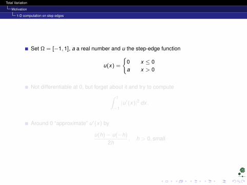
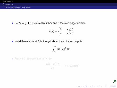
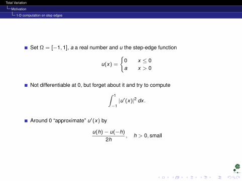
Set Ω = [−1, 1], a a real number and u the step-edge function
u(x) =
0 x ≤ 0a x > 0
Not differentiable at 0, but forget about it and try to compute∫ 1
−1|u′(x)|2 dx .
Around 0 “approximate” u′(x) by
u(h)− u(−h)
2h, h > 0, small
Total Variation
Motivation
1-D computation on step edges
Set Ω = [−1, 1], a a real number and u the step-edge function
u(x) =
0 x ≤ 0a x > 0
Not differentiable at 0, but forget about it and try to compute∫ 1
−1|u′(x)|2 dx .
Around 0 “approximate” u′(x) by
u(h)− u(−h)
2h, h > 0, small
Total Variation
Motivation
1-D computation on step edges
Set Ω = [−1, 1], a a real number and u the step-edge function
u(x) =
0 x ≤ 0a x > 0
Not differentiable at 0, but forget about it and try to compute∫ 1
−1|u′(x)|2 dx .
Around 0 “approximate” u′(x) by
u(h)− u(−h)
2h, h > 0, small
Total Variation
Motivation
1-D computation on step edges
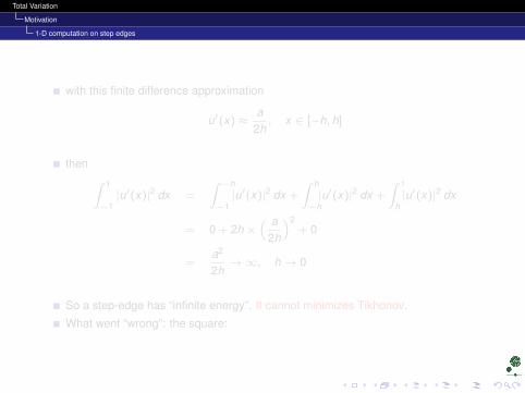
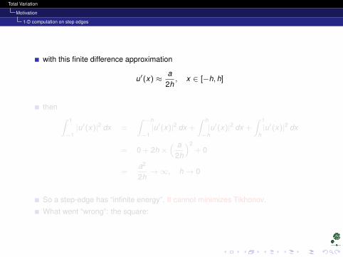
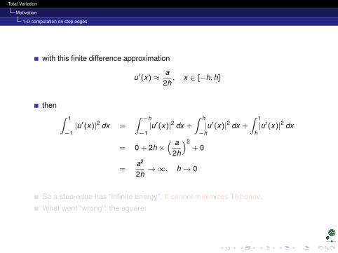
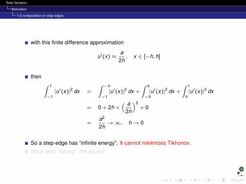
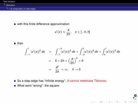
with this finite difference approximation
u′(x) ≈a
2h, x ∈ [−h, h]
then ∫ 1
−1|u′(x)|2 dx =
∫ −h
−1|u′(x)|2 dx +
∫ h
−h|u′(x)|2 dx +
∫ 1
h|u′(x)|2 dx
= 0 + 2h ×( a
2h
)2+ 0
=a2
2h→∞, h→ 0
So a step-edge has “infinite energy”. It cannot minimizes Tikhonov.
What went “wrong”: the square:
Total Variation
Motivation
1-D computation on step edges
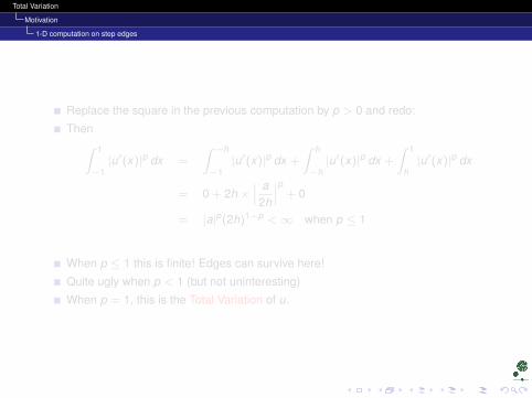
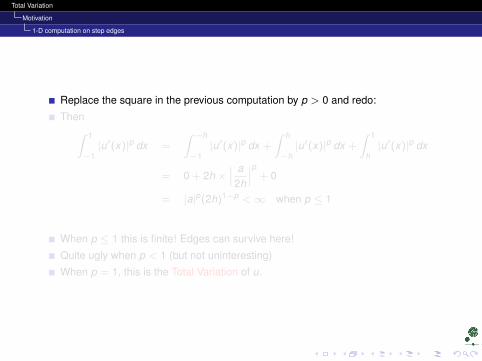
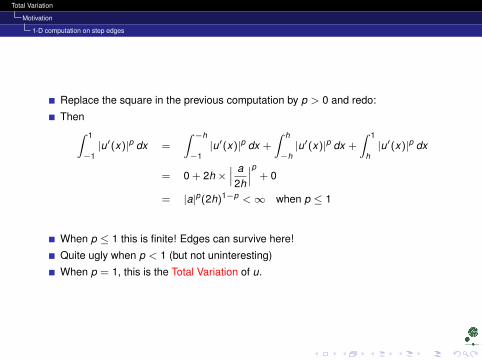
Replace the square in the previous computation by p > 0 and redo:
Then∫ 1
−1|u′(x)|p dx =
∫ −h
−1|u′(x)|p dx +
∫ h
−h|u′(x)|p dx +
∫ 1
h|u′(x)|p dx
= 0 + 2h ×∣∣∣ a2h
∣∣∣p + 0
= |a|p(2h)1−p <∞ when p ≤ 1
When p ≤ 1 this is finite! Edges can survive here!
Quite ugly when p < 1 (but not uninteresting)
When p = 1, this is the Total Variation of u.
Total Variation
Motivation
1-D computation on step edges
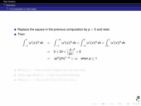
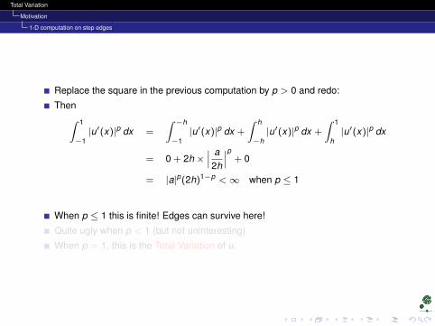
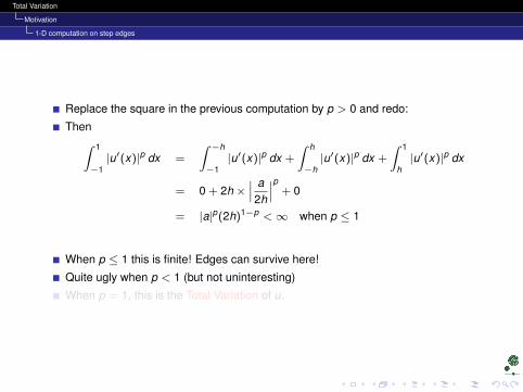
Replace the square in the previous computation by p > 0 and redo:
Then∫ 1
−1|u′(x)|p dx =
∫ −h
−1|u′(x)|p dx +
∫ h
−h|u′(x)|p dx +
∫ 1
h|u′(x)|p dx
= 0 + 2h ×∣∣∣ a2h
∣∣∣p + 0
= |a|p(2h)1−p <∞ when p ≤ 1
When p ≤ 1 this is finite! Edges can survive here!
Quite ugly when p < 1 (but not uninteresting)
When p = 1, this is the Total Variation of u.
Total Variation
Total Variation I
First definition
Outline
1 MotivationOrigin and uses of Total VariationDenoisingTikhonov regularization1-D computation on step edges
2 Total Variation IFirst definitionRudin-Osher-FatemiInpainting/Denoising
3 Total Variation IIRelaxing the derivative constraintsDefinition in actionUsing the new definition in denoising: Chambolle algorithmImage Simplification
4 Bibliography
5 The End
Total Variation
Total Variation I
First definition
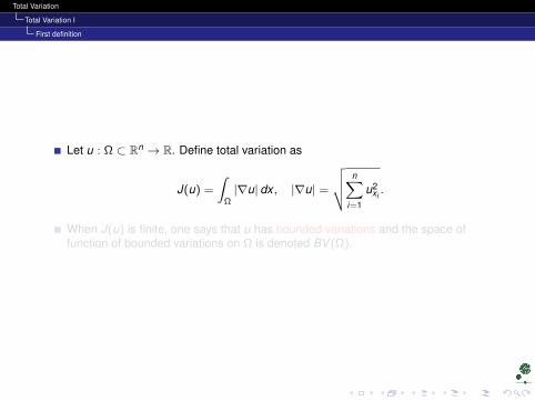
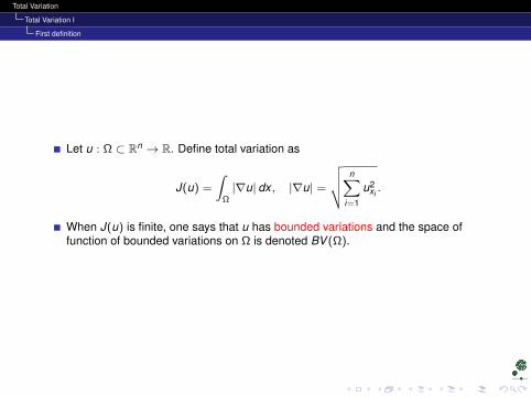
Let u : Ω ⊂ Rn → R. Define total variation as
J(u) =
∫Ω|∇u| dx , |∇u| =
√√√√ n∑i=1
u2xi.
When J(u) is finite, one says that u has bounded variations and the space offunction of bounded variations on Ω is denoted BV (Ω).
Total Variation
Total Variation I
First definition
Let u : Ω ⊂ Rn → R. Define total variation as
J(u) =
∫Ω|∇u| dx , |∇u| =
√√√√ n∑i=1
u2xi.
When J(u) is finite, one says that u has bounded variations and the space offunction of bounded variations on Ω is denoted BV (Ω).
Total Variation
Total Variation I
First definition
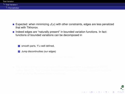
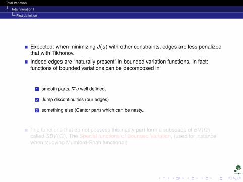
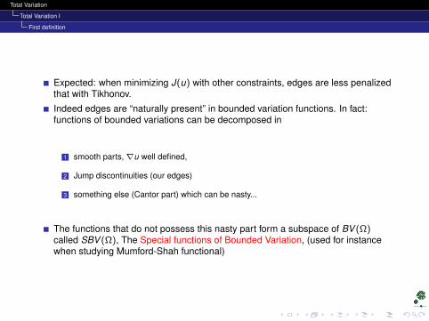
Expected: when minimizing J(u) with other constraints, edges are less penalizedthat with Tikhonov.
Indeed edges are “naturally present” in bounded variation functions. In fact:functions of bounded variations can be decomposed in
1 smooth parts,∇u well defined,
2 Jump discontinuities (our edges)
3 something else (Cantor part) which can be nasty...
The functions that do not possess this nasty part form a subspace of BV (Ω)called SBV (Ω), The Special functions of Bounded Variation, (used for instancewhen studying Mumford-Shah functional)
Total Variation
Total Variation I
First definition
Expected: when minimizing J(u) with other constraints, edges are less penalizedthat with Tikhonov.
Indeed edges are “naturally present” in bounded variation functions. In fact:functions of bounded variations can be decomposed in
1 smooth parts,∇u well defined,
2 Jump discontinuities (our edges)
3 something else (Cantor part) which can be nasty...
The functions that do not possess this nasty part form a subspace of BV (Ω)called SBV (Ω), The Special functions of Bounded Variation, (used for instancewhen studying Mumford-Shah functional)
Total Variation
Total Variation I
Rudin-Osher-Fatemi
Outline
1 MotivationOrigin and uses of Total VariationDenoisingTikhonov regularization1-D computation on step edges
2 Total Variation IFirst definitionRudin-Osher-FatemiInpainting/Denoising
3 Total Variation IIRelaxing the derivative constraintsDefinition in actionUsing the new definition in denoising: Chambolle algorithmImage Simplification
4 Bibliography
5 The End
Total Variation
Total Variation I
Rudin-Osher-Fatemi
ROF Denoising
State the denoising problem as minimizing J(u) under the constraints∫Ω
u dx =
∫Ω
uo dx ,∫
Ω(u − u0)2 dx = |Ω|σ2 (|Ω| = area/volume of Ω)
Solve via Lagrange multipliers.
Total Variation
Total Variation I
Rudin-Osher-Fatemi
ROF Denoising
State the denoising problem as minimizing J(u) under the constraints∫Ω
u dx =
∫Ω
uo dx ,∫
Ω(u − u0)2 dx = |Ω|σ2 (|Ω| = area/volume of Ω)
Solve via Lagrange multipliers.
Total Variation
Total Variation I
Rudin-Osher-Fatemi
ROF Denoising
State the denoising problem as minimizing J(u) under the constraints∫Ω
u dx =
∫Ω
uo dx ,∫
Ω(u − u0)2 dx = |Ω|σ2 (|Ω| = area/volume of Ω)
Solve via Lagrange multipliers.
Total Variation
Total Variation I
Rudin-Osher-Fatemi
TV-denoising
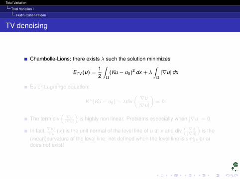
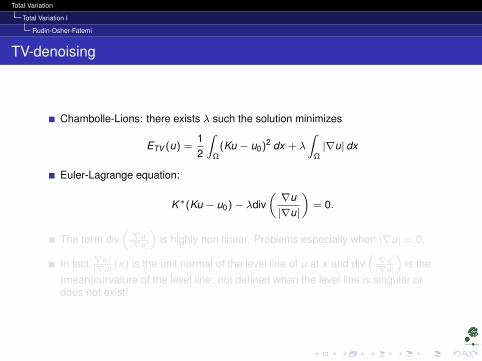
Chambolle-Lions: there exists λ such the solution minimizes
ETV (u) =12
∫Ω
(Ku − u0)2 dx + λ
∫Ω|∇u| dx
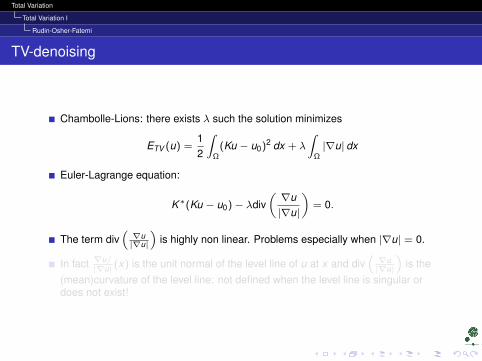
Euler-Lagrange equation:
K∗(Ku − u0)− λdiv(∇u|∇u|
)= 0.
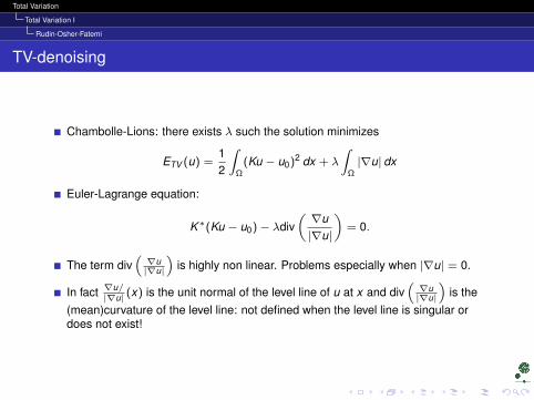
The term div(∇u|∇u|
)is highly non linear. Problems especially when |∇u| = 0.
In fact ∇u/|∇u| (x) is the unit normal of the level line of u at x and div
(∇u|∇u|
)is the
(mean)curvature of the level line: not defined when the level line is singular ordoes not exist!
Total Variation
Total Variation I
Rudin-Osher-Fatemi
TV-denoising
Chambolle-Lions: there exists λ such the solution minimizes
ETV (u) =12
∫Ω
(Ku − u0)2 dx + λ
∫Ω|∇u| dx
Euler-Lagrange equation:
K∗(Ku − u0)− λdiv(∇u|∇u|
)= 0.
The term div(∇u|∇u|
)is highly non linear. Problems especially when |∇u| = 0.
In fact ∇u/|∇u| (x) is the unit normal of the level line of u at x and div
(∇u|∇u|
)is the
(mean)curvature of the level line: not defined when the level line is singular ordoes not exist!
Total Variation
Total Variation I
Rudin-Osher-Fatemi
Acar-Vogel
Replace it by regularized version
|∇u|β =√|∇u|2 + β, β > 0
Acar - Vogel show that
limβ→0
(Jβ(u) =
∫Ω|∇u|β dx
)= J(u).
Replace energy by
E ′(u) =
∫Ω
(Ku − u0)2 dx + λJβ(u)
Euler-Lagrange equation:
K∗(Ku − u0)− λdiv(∇u|∇u|β
)= 0
The null denominator problem disappears.
Total Variation
Total Variation I
Rudin-Osher-Fatemi
Acar-Vogel
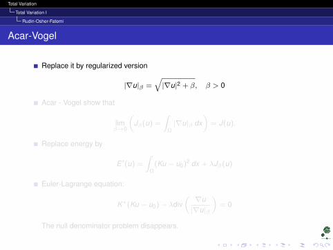
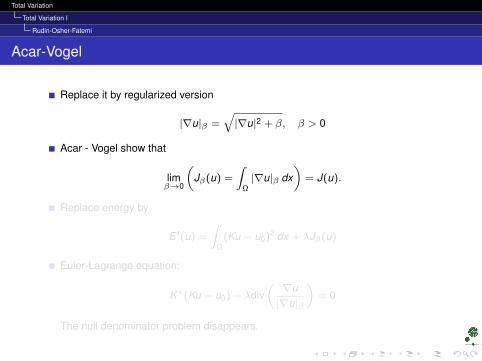
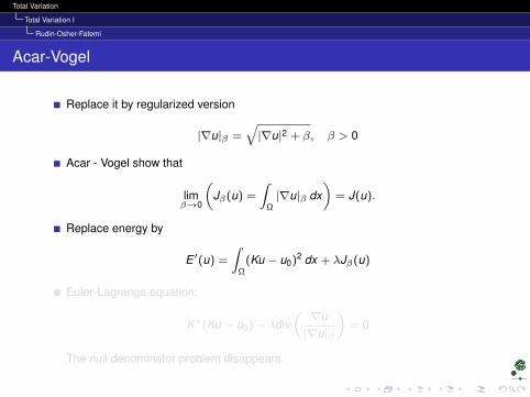
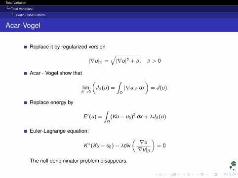
Replace it by regularized version
|∇u|β =√|∇u|2 + β, β > 0
Acar - Vogel show that
limβ→0
(Jβ(u) =
∫Ω|∇u|β dx
)= J(u).
Replace energy by
E ′(u) =
∫Ω
(Ku − u0)2 dx + λJβ(u)
Euler-Lagrange equation:
K∗(Ku − u0)− λdiv(∇u|∇u|β
)= 0
The null denominator problem disappears.

Total Variation
Total Variation I
Rudin-Osher-Fatemi
Example
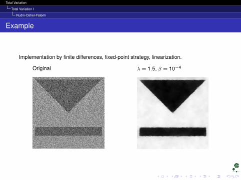
Implementation by finite differences, fixed-point strategy, linearization.
Original λ = 1.5, β = 10−4
Total Variation
Total Variation I
Rudin-Osher-Fatemi
Example
Implementation by finite differences, fixed-point strategy, linearization.
Original λ = 1.5, β = 10−4
Total Variation
Total Variation I
Inpainting/Denoising
Outline
1 MotivationOrigin and uses of Total VariationDenoisingTikhonov regularization1-D computation on step edges
2 Total Variation IFirst definitionRudin-Osher-FatemiInpainting/Denoising
3 Total Variation IIRelaxing the derivative constraintsDefinition in actionUsing the new definition in denoising: Chambolle algorithmImage Simplification
4 Bibliography
5 The End
Total Variation
Total Variation I
Inpainting/Denoising
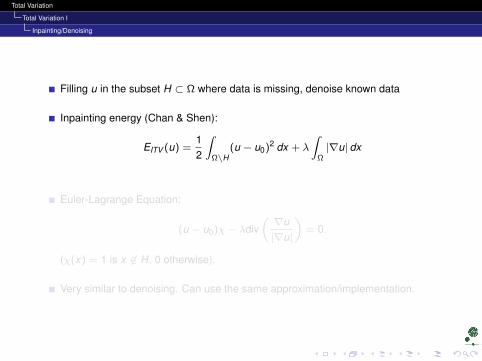
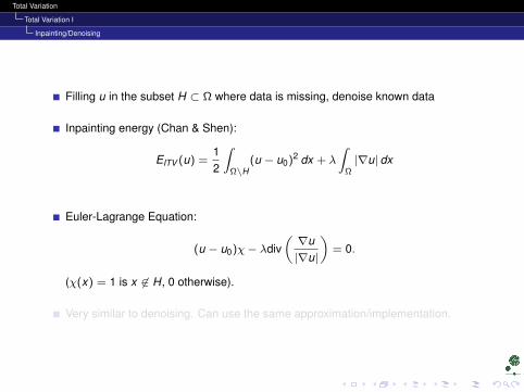
Filling u in the subset H ⊂ Ω where data is missing, denoise known data
Inpainting energy (Chan & Shen):
EITV (u) =12
∫Ω\H
(u − u0)2 dx + λ
∫Ω|∇u| dx
Euler-Lagrange Equation:
(u − u0)χ− λdiv(∇u|∇u|
)= 0.
(χ(x) = 1 is x 6∈ H, 0 otherwise).
Very similar to denoising. Can use the same approximation/implementation.
Total Variation
Total Variation I
Inpainting/Denoising
Filling u in the subset H ⊂ Ω where data is missing, denoise known data
Inpainting energy (Chan & Shen):
EITV (u) =12
∫Ω\H
(u − u0)2 dx + λ
∫Ω|∇u| dx
Euler-Lagrange Equation:
(u − u0)χ− λdiv(∇u|∇u|
)= 0.
(χ(x) = 1 is x 6∈ H, 0 otherwise).
Very similar to denoising. Can use the same approximation/implementation.
Total Variation
Total Variation I
Inpainting/Denoising
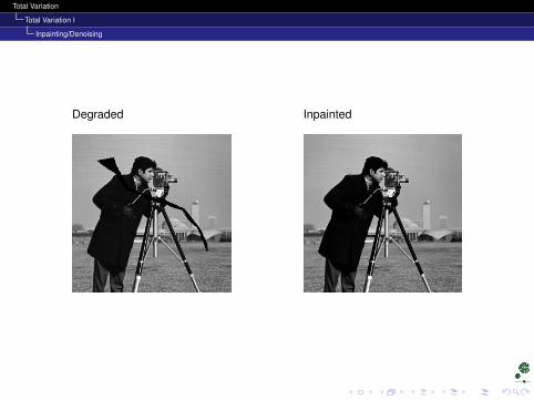
Degraded Inpainted
Total Variation
Total Variation I
Inpainting/Denoising
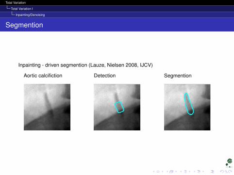
Segmention
Inpainting - driven segmention (Lauze, Nielsen 2008, IJCV)
Aortic calcifiction Detection Segmention
Total Variation
Total Variation II
Relaxing the derivative constraints
Outline
1 MotivationOrigin and uses of Total VariationDenoisingTikhonov regularization1-D computation on step edges
2 Total Variation IFirst definitionRudin-Osher-FatemiInpainting/Denoising
3 Total Variation IIRelaxing the derivative constraintsDefinition in actionUsing the new definition in denoising: Chambolle algorithmImage Simplification
4 Bibliography
5 The End
Total Variation
Total Variation II
Relaxing the derivative constraints
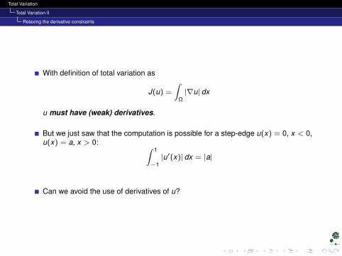
With definition of total variation as
J(u) =
∫Ω|∇u| dx
u must have (weak) derivatives.
But we just saw that the computation is possible for a step-edge u(x) = 0, x < 0,u(x) = a, x > 0: ∫ 1
−1|u′(x)| dx = |a|
Can we avoid the use of derivatives of u?
Total Variation
Total Variation II
Relaxing the derivative constraints
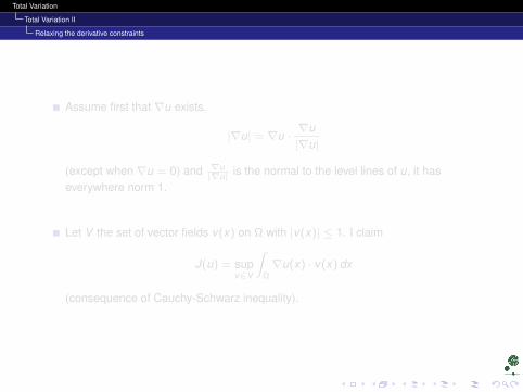
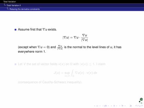
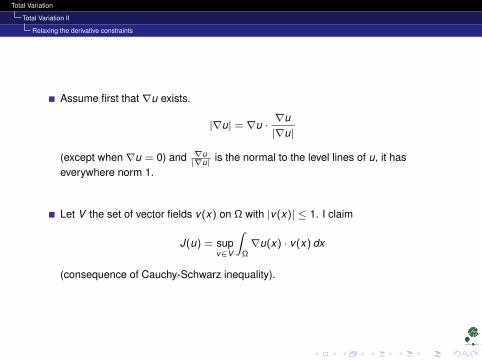
Assume first that ∇u exists.
|∇u| = ∇u ·∇u|∇u|
(except when ∇u = 0) and ∇u|∇u| is the normal to the level lines of u, it has
everywhere norm 1.
Let V the set of vector fields v(x) on Ω with |v(x)| ≤ 1. I claim
J(u) = supv∈V
∫Ω∇u(x) · v(x) dx
(consequence of Cauchy-Schwarz inequality).
Total Variation
Total Variation II
Relaxing the derivative constraints
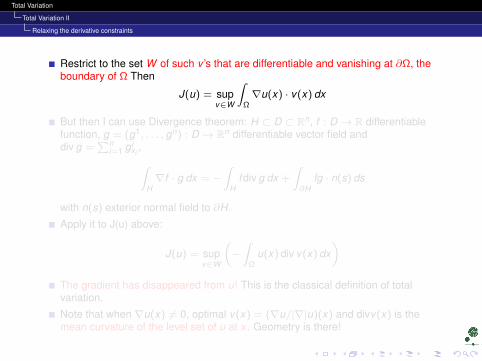
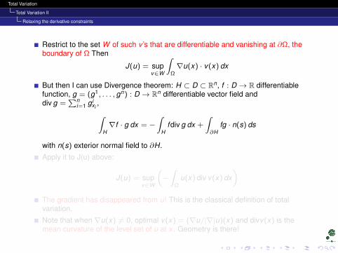
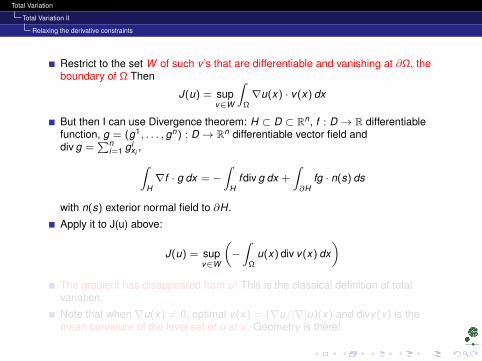
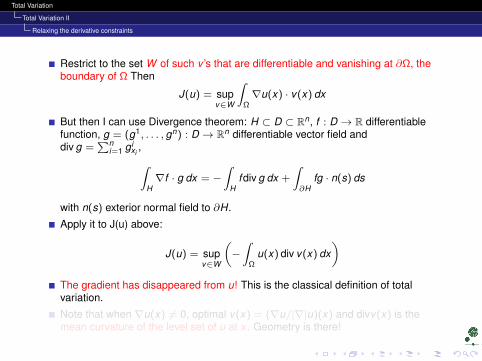
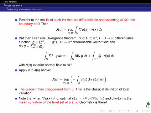
Restrict to the set W of such v ’s that are differentiable and vanishing at ∂Ω, theboundary of Ω Then
J(u) = supv∈W
∫Ω∇u(x) · v(x) dx
But then I can use Divergence theorem: H ⊂ D ⊂ Rn, f : D → R differentiablefunction, g = (g1, . . . , gn) : D → Rn differentiable vector field anddiv g =
∑ni=1 g i
xi,∫
H∇f · g dx = −
∫H
fdiv g dx +
∫∂H
fg · n(s) ds
with n(s) exterior normal field to ∂H.
Apply it to J(u) above:
J(u) = supv∈W
(−∫
Ωu(x) div v(x) dx
)The gradient has disappeared from u! This is the classical definition of totalvariation.
Note that when ∇u(x) 6= 0, optimal v(x) = (∇u/|∇|u)(x) and divv(x) is themean curvature of the level set of u at x . Geometry is there!
Total Variation
Total Variation II
Relaxing the derivative constraints
Restrict to the set W of such v ’s that are differentiable and vanishing at ∂Ω, theboundary of Ω Then
J(u) = supv∈W
∫Ω∇u(x) · v(x) dx
But then I can use Divergence theorem: H ⊂ D ⊂ Rn, f : D → R differentiablefunction, g = (g1, . . . , gn) : D → Rn differentiable vector field anddiv g =
∑ni=1 g i
xi,∫
H∇f · g dx = −
∫H
fdiv g dx +
∫∂H
fg · n(s) ds
with n(s) exterior normal field to ∂H.
Apply it to J(u) above:
J(u) = supv∈W
(−∫
Ωu(x) div v(x) dx
)The gradient has disappeared from u! This is the classical definition of totalvariation.
Note that when ∇u(x) 6= 0, optimal v(x) = (∇u/|∇|u)(x) and divv(x) is themean curvature of the level set of u at x . Geometry is there!
Total Variation
Total Variation II
Definition in action
Outline
1 MotivationOrigin and uses of Total VariationDenoisingTikhonov regularization1-D computation on step edges
2 Total Variation IFirst definitionRudin-Osher-FatemiInpainting/Denoising
3 Total Variation IIRelaxing the derivative constraintsDefinition in actionUsing the new definition in denoising: Chambolle algorithmImage Simplification
4 Bibliography
5 The End
Total Variation
Total Variation II
Definition in action
Step-edge
u the step-edge function defined in previous slides. We compute J(u) with thenew definition.
here W = φ : [−1, 1]→ R differentiable, φ(−1) = φ(1) = 0, |φ(x)| ≤ 1,
J(u) = supφ∈W
∫ 1
−1u(x)φ′(x) dx
we compute ∫ 1
−1u(x)φ′(x) dx = a
∫ 1
0φ′(x) dx
= a (φ(1)− φ(0))
= −aφ(0)
As −1 ≤ φ(0) ≤ 1, the maximum is |a|.
Total Variation
Total Variation II
Definition in action
2D example
B open set with regular boundary curve partialB, Ω large enough to contain B andχB the characteristic function of B
χB(x) =
1 x ∈ B0 x 6∈ B
For v ∈ W , by the divergence theorem on B and its boundary ∂B∫Ωχ(x)div v(x) dx =
∫B
div v(x) dx
= −∫∂B
v(s) · n(s) ds
(n(s) is the exterior normal to ∂B)
This integral is maximized when v = −n : length of ∂B perimeter of B.
Total Variation
Total Variation II
Definition in action
Sets of finite perimeter
Let H ⊂ Ω. If its characteristic function χH satisfies
J(χH ) <∞
H is called set of finite perimeter (and PerΩ(H) := J(χH ) is its perimeter)
This is used for instance in the Chan and Vese algorithm.
If J(u) <∞ and Ht = x ∈ Ω, u(x) < t the lower t-level set of u,
J(u) =
∫ +∞
−∞J(χHt ) dt Coarea formula
Total Variation
Total Variation II
Using the new definition in denoising: Chambolle algorithm
Outline
1 MotivationOrigin and uses of Total VariationDenoisingTikhonov regularization1-D computation on step edges
2 Total Variation IFirst definitionRudin-Osher-FatemiInpainting/Denoising
3 Total Variation IIRelaxing the derivative constraintsDefinition in actionUsing the new definition in denoising: Chambolle algorithmImage Simplification
4 Bibliography
5 The End
Total Variation
Total Variation II
Using the new definition in denoising: Chambolle algorithm
Chambolle algorithm
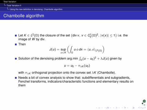
Let K ∈ L2(Ω) the closure of the set div v , v ∈ C10 (Ω)2, |v(x)| ≤ 1 i.e. the
image of W by div.
Then
J(u) = supφ∈K
(∫Ω
u φ dx = 〈u, φ〉L2(Ω)
)Solution of the denoising problem arg.min
∫Ω(u − u0)2 + λJ(u) given by
u = u0 − πλK (u0)
with πλK orthogonal projection onto the convex set λK (Chambolle).
Needs a bit of convex analysis to show that: subdifferentials and subgradients,Fenchel transforms, indicators/characteristic functions and elementary results onthem
Total Variation
Total Variation II
Using the new definition in denoising: Chambolle algorithm
Chambolle algorithm
Let K ∈ L2(Ω) the closure of the set div v , v ∈ C10 (Ω)2, |v(x)| ≤ 1 i.e. the
image of W by div.
Then
J(u) = supφ∈K
(∫Ω
u φ dx = 〈u, φ〉L2(Ω)
)Solution of the denoising problem arg.min
∫Ω(u − u0)2 + λJ(u) given by
u = u0 − πλK (u0)
with πλK orthogonal projection onto the convex set λK (Chambolle).
Needs a bit of convex analysis to show that: subdifferentials and subgradients,Fenchel transforms, indicators/characteristic functions and elementary results onthem
Total Variation
Total Variation II
Using the new definition in denoising: Chambolle algorithm
Fenchel Transform
X Hilbert space, f : X → R convex, proper. Fenchel transform of F :
F∗(v) = supu∈X
(〈u, v〉X − F (u))
Geometric meaning: take u∗ such that F∗(u∗) < +∞: the affine function
a(u) = 〈u, u∗〉 − F∗(u∗)
is tangent to F and a(0) = −F∗(u∗).
Total Variation
Total Variation II
Using the new definition in denoising: Chambolle algorithm
Fenchel transform
Interesting properties:Convexif Φ is the transform of F and λ > 0, then the transform of u 7→ λF (λ−1(u) is λΦ.if F 1-homogeneous, i.e. F (λu) = λF (u) then F∗(u) only take values 0 and +∞ as theproperty above implies F∗ = λF∗, λ > 0.In that case, the set where F∗ = 0 i a closed convex set of X , F∗ = δC , the indicatorfunction of C,
δC (x) =
0 , x ∈ C+∞ , x 6∈ C
For x ∈ R 7→ |x|, C = [−1, 1]For J(u), C = K .
Total Variation
Total Variation II
Using the new definition in denoising: Chambolle algorithm
Subdifferentials
subdifferential of F at u: ∂F (u) = v ∈ X ,F (w)− F (u) ≥ 〈w − u, v〉, ∀w ∈ X.v ∈ ∂F (u) is a subgradient of F at u.Three fundamental (and easy) properties:
0 ∈ ∂F (u) iff u global minimizer of Fu∗ ∈ ∂F (u)⇔ F (u) + F∗(u∗) = 〈u, u∗〉Duality: u∗ ∈ ∂F (u)⇔ u ∈ ∂F∗(u)
The duality above allows to transform optimization of homogeneous functions intodomain constraints!
Total Variation
Total Variation II
Using the new definition in denoising: Chambolle algorithm
TV-denoising
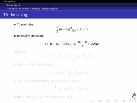
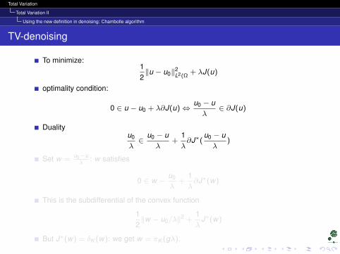
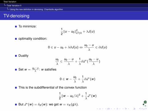
To minimize:12‖u − u0‖2
L2(Ω+ λJ(u)
optimality condition:
0 ∈ u − u0 + λ∂J(u)⇔u0 − uλ
∈ ∂J(u)
Dualityu0
λ∈
u0 − uλ
+1λ∂J∗(
u0 − uλ
)
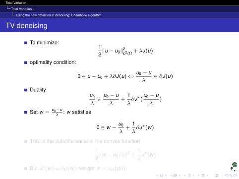
Set w =u0−uλ
: w satisfies
0 ∈ w −u0
λ+
1λ∂J∗(w)
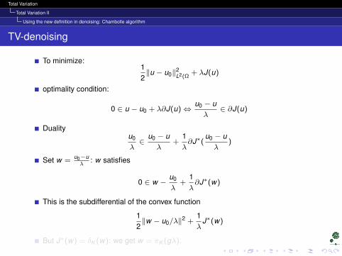
This is the subdifferential of the convex function
12‖w − u0/λ‖2 +
1λ
J∗(w)
But J∗(w) = δK (w): we get w = πK (gλ).
Total Variation
Total Variation II
Using the new definition in denoising: Chambolle algorithm
TV-denoising
To minimize:12‖u − u0‖2
L2(Ω+ λJ(u)
optimality condition:
0 ∈ u − u0 + λ∂J(u)⇔u0 − uλ
∈ ∂J(u)
Dualityu0
λ∈
u0 − uλ
+1λ∂J∗(
u0 − uλ
)
Set w =u0−uλ
: w satisfies
0 ∈ w −u0
λ+
1λ∂J∗(w)
This is the subdifferential of the convex function
12‖w − u0/λ‖2 +
1λ
J∗(w)
But J∗(w) = δK (w): we get w = πK (gλ).
Total Variation
Total Variation II
Using the new definition in denoising: Chambolle algorithm
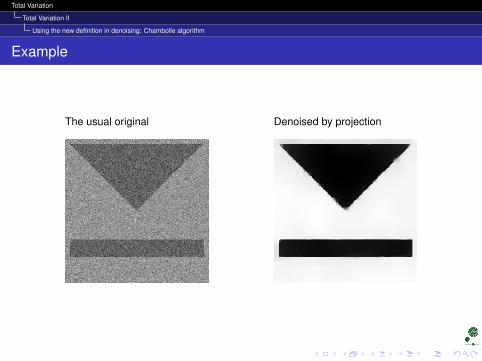
Example
The usual original Denoised by projection
Total Variation
Total Variation II
Image Simplification
Outline
1 MotivationOrigin and uses of Total VariationDenoisingTikhonov regularization1-D computation on step edges
2 Total Variation IFirst definitionRudin-Osher-FatemiInpainting/Denoising
3 Total Variation IIRelaxing the derivative constraintsDefinition in actionUsing the new definition in denoising: Chambolle algorithmImage Simplification
4 Bibliography
5 The End
Total Variation
Total Variation II
Image Simplification
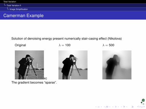
Camerman Example
Solution of denoising energy present numerically stair-casing effect (Nikolova)
Original
xc
λ = 100 λ = 500
The gradient becomes “sparse”.
Total Variation
Bibliography
Bibliography
Tikhonov, A. N.; Arsenin, V. Y. 1977. Solution of Ill-posed Problems.
Wahba, G, 1990. Spline Models for Observational Data.
Rudin, L.; Osher, S.; Fatemi, E. 1992. Nonlinear Total Variation Based NoiseRemoval Algorithms.
Chambolle, A. 2004. An algorithm for Total Variation Minimization andApplications.
Nikolova, M. 2004. Weakly Constrained Minimization: Application to theEstimation of Images and Signals Involving Constant Regions
Total Variation
The End
The End
Recommended