Three Essays in Commodity Futures and Options Price Performance
by
Marin Božić
A dissertation submitted in partial fulfillment of
the requirements for the degree of
Doctor of Philosophy
(Agricultural and Applied Economics)
at the
UNIVERSITY OF WISCONSIN-MADISON
2011

i
Acknowledgements
A single name may stand on the front page of this thesis, but more than a few mentors, teachers and
friends were the influence, support and inspiration without which this endeavor could hardly be
completed, and perhaps not even be embarked upon. First, I want to express my gratitude to my advisor,
Dr. T. Randall Fortenbery, who has supervised this work over the past three years, and has provided me
with essential financial and intellectual support. Randy’s understanding of commodity markets is without
par, and through many debates he has challenged me to think more deeply, write more clearly and has
corrected more omitted definite articles in my drafts than I would like to admit.
I have also benefited immensely from discussions with Professors Jean-Paul Chavas, Brian W. Gould,
Bruce E. Hansen and James E. Hodder. I am deeply thankful for their willingness to serve on my PhD
thesis committee and read through early drafts of these essays. Their substantial scholarly contributions,
sharp intellectual instincts and, above all, kind nature and spirit illuminate all students fortunate to be able
to work with them.
A special thanks goes to my colleagues and friends at The Institute of Economics, Zagreb where I started
my post-college career before coming to US for graduate studies. Without the encouragement I got from
Dr. Nenad Starc, the head of my division and a dear mentor and friend, and Dr. Sandra Švaljek, the
Director of the Institute, America would perhaps remain only a dream. Financial support of the Institute
allowed me, among other things, to visit Croatia each summer and present my work at a workshop in
Zagreb.
A unique influence to my thinking, and an unfading inspiration in integrity, Dr. Ivo Bićanić of the Faculty
of Economics at the University of Zagreb, more than any other single person, set me on the path I thread
today. I keenly remember one lecture on macroeconomics of Croatia where he scolded me in front of the

ii
entire class for not paying attention – and even the fact that I was at that moment reading his own newly
published article did not help!
My parents, my brother, and my late grandma were with me from the beginning of my graduate studies,
through all my efforts and many Skype conversations that were often more successful at conveying their
love than clear audio of their voice. By ourselves, we are a bunch of headstrong individuals, but together
we share deep trust and unyielding silent support that gives space when space is asked for, and support
when support is needed.
This acknowledgement would be unforgivingly incomplete if I do not mention Josip Glaurdić, my dear
friend since high school days, who set the bar as the first kid I knew that went to the USA to study;
Jeremy Weber, a genius of balanced life and an unmatched dedicated spirit; and, Dan Prager, with whom
I shared many nice moments discussing with much passion issues both deep and shallow, U.S. politics
being often the latter.
Finally, I dedicate this thesis to my partner and my best friend, Debanjana Chatterjee. Others may benefit
from this work, but she has borne most of the cost. Through all-nighters spent over Gauss code and many
precious moments of peace I chose to forfeit in pursuit of my degree, she has given me her full heart and
mind, and I am forever grateful for her support, patience and wisdom.
iii
List of Figures
Figure 1.1. Typical Pattern for Implied Volatility Coefficients for Options on Agricultural Futures ....... 38
Figure 1.2. Evolution of Implied Volatility Curve for Options on Dec’ 04 and Dec ’06 Corn Futures. ... 39
Figure 1.3. Effects of Excess Kurtosis and Positive Skewness on Implied Volatility ............................... 40
Figure 1.4. New Crop Price Distributions Conditional on Storage Adequacy .......................................... 41
Figure 1.5. Weather Stress in the Corn Crop ............................................................................................. 41
Figure 1.6. Monthly Projected Corn Yield 1980-2008 - Deviation from Trend ........................................ 42
Figure 1.7. Monthly Projected Corn Yield 1980-2008 - Deviation from the Final Estimate (January) .... 42
Figure 1.8. Options on Corn Futures: Dynamics of Implied Skewness ..................................................... 43
Figure 1.9. Relationship between Implied Skewness and Expected Ending Stocks-to-Use ...................... 44
Figure 1.10. Predicted Intra-Year Dynamics of Implied Skewness for Options on Corn Futures Contracts
.................................................................................................................................................................... 45
Figure 2.1. Manufacturing Milk Price: 1970-2009 .................................................................................... 88
Figure 1.2. Class III Milk futures - Partially Overlapping Time Series vs. “Nearby” Series .................... 89
Figure 2.3. Class III Milk Futures: Open Interest and Nearby Price 2000-2009. ...................................... 90
Figure 2.4. Realized Prediction Errors of Class III Milk Futures Prices. .................................................. 91
Figure 12.5. Class III Milk Futures: Unconditional Standard Deviation of Price Change as a Function of
Time to Maturity. ........................................................................................................................................ 92
Figure 2.6. Proportion of Variance Explained by the Common Factor. .................................................... 93
Figure 2.7. Common Factor Importance for Class III Milk Futures. ......................................................... 94
Figure 2.8. Proportion of Market Variance Explained by the Common Factor. ........................................ 95
Figure 2.9. U.S. Commercial Dairy Cow Slaughter, Percentage of Annual Cull. ..................................... 96
Figure 2. 110. Manufacturing Milk Price: Sample Spectrum (Jan 1970-Apr 1991). .................................. 97
Figure 2.11. Manufacturing Milk Price: Sample Spectrum (Sep 1988-Dec 2009). ................................... 98
Figure 3.1. Flowchart Diagram of Classified Milk Pricing in Federal Milk Marketing Orders .............. 160
Figure 3.2. Calculating Implied Cheese Futures Price ............................................................................. 161
Figure 3.3. Implied vs. Observed Cheese Futures ................................................................................... 162
Figure 3.4. Average Absolute Value of Cheese Cash-Futures Spread, as a Function of Time to Maturity.
.................................................................................................................................................................. 163
Figure 3.5. Percentage Net Long Positions for all Trader Groups ............................................................ 164
iv
List of Tables
Table 1.1. Determinants of Implied Skewness: Descriptive Statistics ....................................................... 46
Table 1.2. Corn Supply/Demand Balance Sheet 1995-2009 ....................................................................... 47
Table 1.3. Models of Intra-Year Skewness Dynamics: Regression Results .............................................. 49
Table 1.4. Relative Contribution of Corn Growth-Sensitive Period to Reduction in Implied Skewness .. 50
Table 1.5. Determinants of Implied Skewness: Regression Results .......................................................... 51
Table 2.1. Specifications of Dairy Futures Contracts. ............................................................................... 99
Table 2.2. Dairy Prices: Correlations 2000-2009..................................................................................... 100
Table 2.3. Determination of Manufacturing Grade Milk Price in Federal Milk Marketing Orders ........ 101
Table 2.4. Class III Futures: Proportion of Variance Explained by the Common Factor. ....................... 102
Table 3.1. Unit Root Tests ....................................................................................................................... 165
Table 3.2. Simple Error-Correction Model: Comparing Results Across Data Frequency and Cash Series
Type .......................................................................................................................................................... 166
Table 3.3. Simple Error-Correction Model: Comparing Results Across Data Frequency and Cash Series
Type – Log-Prices ..................................................................................................................................... 167
Table 3.4. Volatility Spillovers ................................................................................................................ 168
Table 3.5. Evaluating Adequacy of Speculation in Cheese Futures Market: Selected Results from
GARCH-MEX Model ............................................................................................................................... 169

v
THREE ESSAYS IN COMMODITY FUTURES AND OPTIONS PRICE PERFORMANCE
Marin Božić
Under the supervision of RENK Professor of Agribusiness T. Randall Fortenbery
At the University of Wisconsin-Madison
Abstract
In the first essay I propose a novel pricing model for options on commodity futures motivated
from the economic theory of optimal storage, and consistent with implications of plant
physiology on the importance of weather stress. The model is based on a Generalized Lambda
Distribution (GLD) that allows greater flexibility in higher moments of the expected terminal
distribution of futures price. I find a statistically significant negative relationship between ending
stocks-to-use and implied skewness, as predicted by the theory of storage. Intra-year dynamics of
implied skewness reflect the fact that resolution of uncertainty in corn supply is resolved during
the corn growth phase from corn silking through maturity. Impacts of storage and weather on the
distribution of terminal futures prices jointly explain upward sloping implied volatility curves.
In the second paper, a partially overlapping time series (POTS) model is estimated to examine
price behavior in simultaneously traded Class III milk futures contracts. POTS is a latent factor
model that measures price changes in futures as a linear combination of a common factor, i.e.
information affecting all traded contracts, and an idiosyncratic term specific to each contract.
The importance of a common factor in price volatility determination for dairy is related to capital
production factors, i.e. the dairy herd. It is shown that Class III volatility decreases as contracts
approach maturity. The importance of the common factor declines as one approaches maturity,
implying that individual contract months are poor substitutes in hedging a specific month’s cash
vi
price risk. Thus, despite relatively low liquidity in the market, it is useful to have 12 contract
delivery months per year.
The third essay examines price discovery, volatility spillovers and the impacts of speculation in
the dairy sector. I find that the flow of information in the mean prices is predominantly from
futures to cash, while volatility spillovers are bidirectional. I propose an extension of the BEKK
variance model that I refer to as GARCH-MEX. Utilizing the model to evaluate the impact of
speculation I find strong evidence against the hypothesis that excessive speculation is increasing
the conditional variance of futures prices.
vii
Table of Contents
Acknowledgements ........................................................................................................................................ i
List of Figures .............................................................................................................................................. iii
List of Tables ............................................................................................................................................... iv
Abstract ......................................................................................................................................................... v
1. Pricing Options on Commodity Futures: The Role of Weather and Storage ........................................ 1
1.1. Introduction ................................................................................................................................... 2
1.2. Theory ........................................................................................................................................... 3
1.2.1. Foundations of Arbitrage Pricing Theory for Options on Futures ........................................ 3
1.2.2. Storage and Time-series Properties of Commodity Spot and Futures Prices ........................ 9
1.2.3. The Role of Weather in Intra-year Resolution of Price Uncertainty ................................... 12
1.2.4. Option Pricing Formula Using Generalized Lambda Distribution ..................................... 13
1.3. Econometric Model ..................................................................................................................... 16
1.3.1. Estimating Implied Skewness ............................................................................................. 16
1.3.2. Modeling Intra-year Dynamics of Implied Skewness ......................................................... 18
1.3.3. Inter-year Variation of Implied Skewness .......................................................................... 22
1.4. Data ............................................................................................................................................. 24
1.5. Estimation Procedure and Results ............................................................................................... 25
1.5.1. Estimating Parameters of GLD Distribution and Implied Higher Moments....................... 25
1.5.2. Dynamics of Intra-year Implied Skewness: Results ........................................................... 27
1.5.3. Intra-year Variation in Implied Skewness: Results ............................................................. 32
1.6. Conclusions and Further Research .............................................................................................. 33
1.7. References ................................................................................................................................... 35
2. Volatility Dynamics in Non-storable Commodities: A Case of Class III Milk Futures ..................... 52
2.1. Introduction ................................................................................................................................. 53
2.2. Overview of Dairy Futures Contracts ......................................................................................... 55
2.2.1. Evolution of Dairy Futures ................................................................................................. 55
2.2.2. Price Relationships among Current Contracts .................................................................... 57
2.3. Literature Review ........................................................................................................................ 58
2.4. Econometric Analysis ................................................................................................................. 60
2.4.1. The POTS Model - Introduction ......................................................................................... 60
viii
2.4.2. Using Kalman Filter to Obtain Conditional Variance of the Common Factor ................... 64
2.4.3. Estimating POTS Model ..................................................................................................... 67
2.5. Data ............................................................................................................................................. 70
2.6. Results ......................................................................................................................................... 72
2.7. Conclusions ................................................................................................................................. 79
2.8. Appendix 1. Spectral Analysis of Manufacturing Milk Prices ................................................... 81
2.9. Appendix 2. POTS Estimation Results ....................................................................................... 82
2.10. References ............................................................................................................................... 86
3. Price Discovery, Volatility Spillovers and Adequacy of Speculation in Cheese Spot and Futures Markets ..................................................................................................................................................... 103
3.1. Introduction ............................................................................................................................... 104
3.2. Literature Review ...................................................................................................................... 106
3.3. Data ........................................................................................................................................... 110
3.4. Time Series Properties of Cheese Cash and Futures Prices. ..................................................... 117
3.4.1. Unit Root Tests ................................................................................................................. 118
3.4.2. Economic Theory and Time Series Properties of Agricultural Cash and Futures Prices .. 123
3.5. Information flows between cheese cash and futures markets ................................................... 131
3.5.1. Concepts of Causality ....................................................................................................... 132
3.5.2. Testing for Second-Order Non-Causality ......................................................................... 134
3.5.3. Model for Evaluating Information Flows Between Cash and Futures Cheese Prices. ...... 136
3.5.4. Measures of Speculative Adequacy .................................................................................. 143
3.6. Model Results ........................................................................................................................... 148
3.7. Conclusions and Directions for Future Research ...................................................................... 151
3.8. References ................................................................................................................................. 155

1
1. Pricing Options on Commodity Futures: The Role of Weather and Storage
Abstract: Options on agricultural futures are popular financial instruments used for agricultural
price risk management and to speculate on future price movements. Poor performance of Black’s
classical option pricing model has stimulated many researchers to introduce pricing models that
are more consistent with observed option premiums. However, most models are motivated solely
from the standpoint of the time series properties of futures prices and need for improvements in
forecasting and hedging performance. In this paper I propose a novel arbitrage pricing model
motivated from the economic theory of optimal storage, and consistent with implications of plant
physiology on the importance of weather stress. I introduce a pricing model for options on
futures based on a Generalized Lambda Distribution (GLD) that allows greater flexibility in
higher moments of the expected terminal distribution of futures price. I use times and sales data
for corn futures and options for the period 1995-2009 to estimate the implied skewness
parameter separately for each trading day. An economic explanation is then presented for inter-
year variations in implied skewness consistent with the theory of storage. After controlling for
changes in planned acreage, I find a statistically significant negative relationship between ending
stocks-to-use and implied skewness, as predicted by the theory of storage. Furthermore, intra-
year dynamics of implied skewness reflect the fact that resolution of uncertainty in corn supply is
resolved between late June and middle of October, i.e. during corn growth phases that
encompass corn silking through grain maturity. Impacts of storage and weather on the
distribution of terminal futures price jointly explain upward sloping implied volatility curves.
JEL Codes: G13, Q11, Q14
Keywords: arbitrage pricing model, options on futures, generalized lambda distribution, theory of storage, skewness

2
1.1. Introduction
Options written on commodity futures have been investigated from several aspects in the
commodity economics literature. For example, Lence (1994), Vercammen (1995), Lien and
Wong (2002), and Adam-Müller and Panaretou (2009) considered the role of options in optimal
hedging. Use of options in agricultural policy was examined by Gardner (1977), Glauber and
Miranda (1989), and Buschena (2008). The effects of news on options prices has been
investigated by Fortenbery and Sumner (1993), Isengildina-Massa, Irwin, Good, and Gomez
(2008) and Thomsen (2009). The informational content of options prices has been looked into by
Fackler and King (1990), Sherrick, Garcia and Tirupattur (1996), and Egelkraut, Garcia, and
Sherrick (2007). Some of the most interesting work done in this area considers modifications to
the standard Black-Scholes formula that accounts for non-normality (skewness, leptokurtosis) of
price innovations, heteroskedasticity, and specifics of commodity spot prices (e.g. mean-
reversion). Examples include Kang and Brorsen (1995), and Ji and Brorsen (2009).
In this article I revisit the well-known fact that the classical Black’s (1976) model is inconsistent
with observed option premiums. Previous studies like Fackler and King (1990) and Sherrick et
al. (1996) address this puzzle by identifying properties of futures prices that deviate from
assumptions of Black’s model, i.e. leptokurtic and skewed distributions of the logarithm of
terminal futures prices and stochastic volatility. A common feature of past studies is the
grounding of their arguments in the time-series properties of stochastic processes for futures
prices and the distributional properties of terminal futures prices. In other words, their arguments
are primarily statistical. In contrast to previous studies, I offer an economic explanation for the
observed statistical characteristics. In this paper I analyze in detail options on corn futures. The
focus is on presenting an alternative pricing model that is not motivated by improving the
3
forecasts of options premiums compared to Black’s or other models, but by linking option
pricing models with the economics of supply for annually harvested storable agricultural
commodities. In particular, I demonstrate the effect of storability and crop physiology (i.e.
susceptibility to weather stress) on higher moments of the futures price distribution. Only by
understanding these fundamental economic forces can I truly explain why classical option
pricing models work so poorly for commodity futures.
The article is organized as follows. In the next section I examine in detail the implications of
Black’s classical option pricing model on the shape and dynamics of the futures price
distribution. I follow by summarizing the rational expectations competitive equilibrium model
with storage (Williams and Wright,1991; Deaton and Laroque, 1992), and a testable hypothesis
on conditional new crop price distributions that follows from those models. In addition to
storage, I present the agronomical research on the impact of weather on corn yields. I then
develop a novel arbitrage pricing model for options on commodity futures based on the
Generalized Lambda Distribution (GLD) which I propose to use in calibrating skewness of new
crop futures price to match observed option premiums. The third section describes the
econometric model. In the fourth section I summarize the data used in econometric analysis.
Finally, I describe the estimation procedure and present results of statistical inference, followed
by a set of conclusions and directions for further research.
1.2. Theory
1.2.1. Foundations of Arbitrage Pricing Theory for Options on Futures
Black (1976) was the first to offer an arbitrage pricing model for options on futures contracts.
Despite numerous extensions and modifications proposed in the literature, and the inability of the
model to explain observed option premiums, traders still use this model in practice. This is likely
4
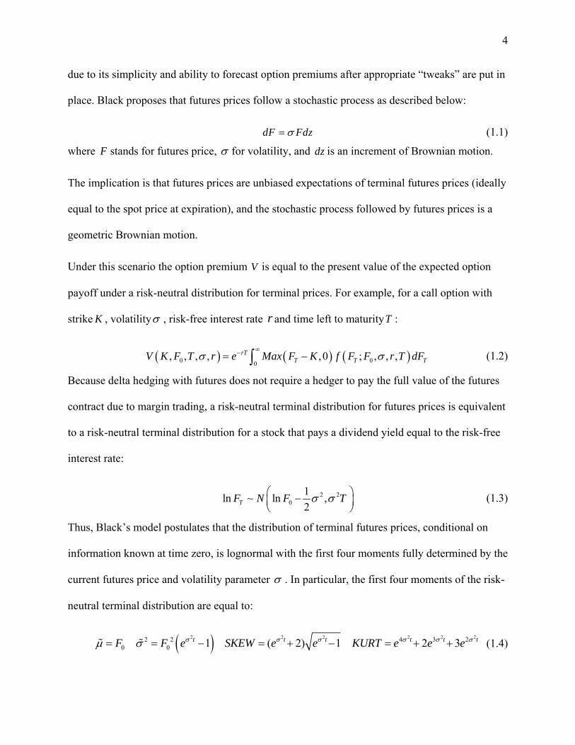
due to its simplicity and ability to forecast option premiums after appropriate “tweaks” are put in
place. Black proposes that futures prices follow a stochastic process as described below:
dF Fdz (1.1)
where F stands for futures price, for volatility, and dz is an increment of Brownian motion.
The implication is that futures prices are unbiased expectations of terminal futures prices (ideally
equal to the spot price at expiration), and the stochastic process followed by futures prices is a
geometric Brownian motion.
Under this scenario the option premium V is equal to the present value of the expected option
payoff under a risk-neutral distribution for terminal prices. For example, for a call option with
strike K , volatility , risk-free interest rate r and time left to maturityT :
0 00, , , , , 0 ; , , ,rT
T T TV K F T r e Max F K f F F r T dF (1.2)
Because delta hedging with futures does not require a hedger to pay the full value of the futures
contract due to margin trading, a risk-neutral terminal distribution for futures prices is equivalent
to a risk-neutral terminal distribution for a stock that pays a dividend yield equal to the risk-free
interest rate:
2 20
1ln ~ ln ,
2TF N F T
(1.3)
Thus, Black’s model postulates that the distribution of terminal futures prices, conditional on
information known at time zero, is lognormal with the first four moments fully determined by the
current futures price and volatility parameter . In particular, the first four moments of the risk-
neutral terminal distribution are equal to:
2 22 2 2 220
4 320
2( 2) 31 1 2t t t t t tF F e SKEW KUe e e eRT e (1.4)

5
For example, if a futures price is $2.50, volatility is 30%, and there are 160 days left to maturity,
the standard deviation of the terminal distribution would be $0.50, skewness would be 0.60 and
kurtosis would be 3.64. Therefore, the standard Black’s model implies that the expected
distribution of terminal prices would be positively skewed, and leptokurtic. When complaints are
raised that Black’s model imposes normality restrictions, it is the logarithm of the terminal price
that the critique refers to.
The standard way to check if Black’s model is an appropriate pricing strategy is to exploit the
fact that for a given futures price, strike price, risk-free interest rate, and time to maturity, the
model postulates a one-to-one relationship between the volatility coefficient and the option
premium. Thus, the pricing function can be inverted to infer the volatility coefficient from an
observed option premium. Such coefficients are referred to as implied volatility and the principal
testable implication of Black’s model is that implied volatility does not depend on how deep in-
the-money or out-of-money an option is. If the logarithm of terminal price is not normally
distributed, then Black’s model is not appropriate, and implied volatility (IV) will vary with
option moneyness – a flagrant violation of the model’s assumptions. Black’s model gives us a
pricing formula for European options on futures, i.e. options that can only be exercised at
contract maturity. Prices of American options on futures that are assumed to follow the same
stochastic process as in Black’s model must also account for the possibility of early exercise. For
that reason, their prices cannot be obtained through a closed-form formula, but must be estimated
through numerical methods such as the Cox, Ross and Rubinstein (CRR) (1979) binomial trees.
Implied volatility curves for storable commodity products are almost always upward sloping. As
an example consider the December 2006 corn contract. The futures price on June 26, 2006 was
$2.49/bu. As seen in Figure 1.1, the implied volatility curve associated with calculating IV using

6
various December option strikes is strongly upward sloping, with the implied volatility
coefficients for the highest strike options close to 15 percentage points higher than the implied
volatility for options with lower strikes.
Geman (2005) calls this phenomenon an “inverse leverage effect,” after the “leverage effect”
proposed to explain downward sloping implied volatility curves for individual company stocks.
However, this is a complete misnomer. As Black (1976b) explains, the leverage effect arises
from the fact that as stock price declines, the ratio of a company’s debt to equity value, its
leverage, increases. If the volatility of company assets is constant, then as the equity share of
assets declines, volatility in equity will increase. While the leverage effect has a coherent causal
model to justify the term, nothing explains “inverse leverage effect.”
We can gain further insight as to how Black’s model performs if we plot the implied volatility
curve for a single contract at different time-to-maturity horizons. As an example, consider
December corn contracts in the years 2004 and 2006. As Figure 1.2 shows, three distinct patterns
are noticeable. First, except when options are very near maturity, we always see an upward
sloping implied volatility curve. Second, implied volatility of at-the-money options, i.e. options
that have the strike price equal to the current futures price, rises almost linearly until the end of
June, declines throughout the summer months, and then starts rising again. Finally, near
maturity, volatility skews give way to symmetric volatility smiles. The implied volatility
coefficient measures volatility on an annual basis, and the variance of the terminal price,
conditional on time remaining to maturity, is 2 T t . So if uncertainty about the terminal
price is uniformly resolved as time passes, implied volatility will not decrease, but will stay the
same. Likewise, when the same amount of uncertainty needs to be resolved in a shorter time
interval implied volatility will increase. Therefore, linear increases in implied volatility from
7
distant horizons up until June is best interpreted not as increases in day to day volatility of
futures price changes, but a market consensus that the conditional variance of terminal prices is
not much reduced before June.
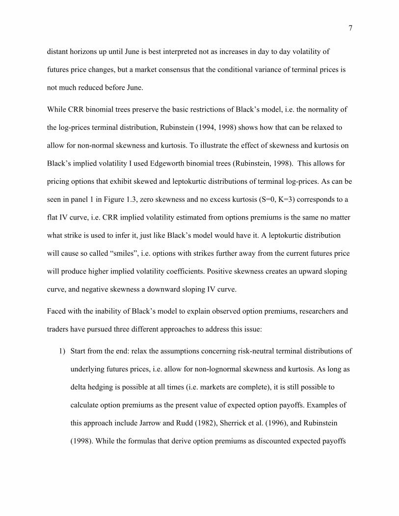
While CRR binomial trees preserve the basic restrictions of Black’s model, i.e. the normality of
the log-prices terminal distribution, Rubinstein (1994, 1998) shows how that can be relaxed to
allow for non-normal skewness and kurtosis. To illustrate the effect of skewness and kurtosis on
Black’s implied volatility I used Edgeworth binomial trees (Rubinstein, 1998). This allows for
pricing options that exhibit skewed and leptokurtic distributions of terminal log-prices. As can be
seen in panel 1 in Figure 1.3, zero skewness and no excess kurtosis (S=0, K=3) corresponds to a
flat IV curve, i.e. CRR implied volatility estimated from options premiums is the same no matter
what strike is used to infer it, just like Black’s model would have it. A leptokurtic distribution
will cause so called “smiles”, i.e. options with strikes further away from the current futures price
will produce higher implied volatility coefficients. Positive skewness creates an upward sloping
curve, and negative skewness a downward sloping IV curve.
Faced with the inability of Black’s model to explain observed option premiums, researchers and
traders have pursued three different approaches to address this issue:
1) Start from the end: relax the assumptions concerning risk-neutral terminal distributions of
underlying futures prices, i.e. allow for non-lognormal skewness and kurtosis. As long as
delta hedging is possible at all times (i.e. markets are complete), it is still possible to
calculate option premiums as the present value of expected option payoffs. Examples of
this approach include Jarrow and Rudd (1982), Sherrick et al. (1996), and Rubinstein
(1998). While the formulas that derive option premiums as discounted expected payoffs
8
assume that options are European, one can still price American options using implied
binomial trees calibrated to the terminal distribution of choice (Rubinstein, 1994).
2) Start from the beginning: start by asking what kind of stochastic process is consistent
with a non-normal terminal distribution? By introducing appropriate stochastic volatility
and/or jumps, one might be able to fit the data just as well as by the approach above.
Examples of this approach are Kang and Brorsen (1995), Hilliard and Reis (1998) and Ji
and Brorsen (2009).
3) “Tweak it so it works good enough” approach: if one is willing to sacrifice mathematical
elegance, the coherence of the second approach, and insights that might emerge from the
first approach, and if the only objective is the ability to forecast day-ahead option
premiums one can simply tweak Black’s model. An example of such an approach would
be to model the implied volatility coefficient as a quadratic function of the strike. Even
though it makes no theoretical sense (this is like saying that options with different strikes
live in different universes), this approach will work good enough for many traders. Just as
in that famous saying by Yogi Berra (2010): “In theory, there is no difference between
theory and practice. In practice, there is.” A seminal article that evaluates the hedging
effectiveness of such an approach is Dumas, Fleming and Whaley (1998). The authors
find that for hedging purposes such an ad-hoc approach seems to work equally well
compared to the more sophisticate and theoretically coherent models they evaluate.
In this article I take the first approach, and modify the Black’s model by modifying the terminal
distribution of futures price. Instead of a lognormal, I propose a generalized lambda distribution
(GLD) developed by Ramberg and Schmeiser (1974) and introduced to options pricing by
Corrado (2001). An alternative would be to use Edgeworth binomial trees, but preliminary
9
analysis showed that such an approach may not be adequate for situations where skewness and
kurtosis are rather high. In addition, Edgeworth trees work with the skewness of terminal log-
prices, while I prefer to have implied parameters for the skewness of terminal futures prices
directly, not their logarithms. In addition, the GLD pricing model allows for a higher degree of
flexibility in terms of skewness and kurtosis, i.e. its’ parameters are rather easy to calibrate from
observed options prices and it is straightforward to develop a closed-form solution for pricing
options. While these are all favorable characteristics, it is in fact the ability to gain additional
economic insight that truly justifies yet another option pricing model. GLD allows us to get an
explicit estimate of skewness and kurtosis of the terminal distributions, that can be used to make
a strong connection between the economics of supply for storable agricultural commodities and
financial models for pricing options on commodity futures. As is usually the case with option
pricing, we are estimating risk-neutral, rather than physical (i.e. true) moments of the price
distribution. In subsequent analysis we assume that all risk-adjustements are contained in the first
moment of the distribution, i.e. the level of a futures price.
1.2.2. Storage and Time-series Properties of Commodity Spot and Futures Prices
Deaton and Laroque (1992) used a rational expectations competitive storage model to explain
nonlinearities in the time series of commodity prices: skewness, rare but dramatic substantial
increases in prices, and a high degree of autocorrelation in prices from one harvest season to the
next. The basic conclusion of their work was that the inability to carry negative inventories
introduces a non-linearity in prices that manifests itself in the above characteristics.
This is an example of theory being employed in an attempt to replicate patterns of observed price
data. In a similar fashion, but subtly different, Williams and Wright (1991) postulate that the
10
moments of expected price distributions at harvest time vary with the current (pre-harvest) price
and available carryout stocks, as shown in Figure 1.4. According to them, when observed at
annual or quarterly frequency, spot prices exhibit positive autocorrelation that emerges because
storage allows unusually high or low excess demand to be spread out over several years.
Furthermore, the variance of price changes depends on the level of inventory. When stocks are
high, and the spot price is low, the abundance of stored stocks serves as a buffer to price
changes, and variance is low. When stocks are low, and thus the spot price is high, stocks are not
sufficient to buffer price changes. Finally, the third moment of the price change distribution also
varies with inventories. Since storage can always reduce the downward price pressure of a
windfall harvest, but cannot do as much for a really bad harvest, large price increases are more
common than large decreases. The magnitude of this cushioning effect of storage depends on the
size of the stocks. In conclusion, one should expect commodity prices to be mean-stationary,
heteroskedastic and with conditional skewness, where both the second and third moments
depend on the size of the inventories.
Testing the theory proceeds with this argument: if we can replicate the price pattern using a
particular set of rationality assumptions, then we cannot refute the claim that markets indeed
behave as described above. That is the road taken by Deaton and Laroque (1992) and Miranda
and Rui (1995). However, since in the spot price series we only see the realizations of prices, not
the conditional expectations of them, we cannot use spot price data to directly test what the
market expected to happen. As such, predictions from storage theory focused on the scale and
shape of expected distributions of new harvest spot prices have remained untested. In this paper I
use options data to infer the conditional expectations of terminal futures prices, and therefore test
the following prediction of the theory of storage:

11
The lower inventories are relative to consumption, the more positive will be the skewness
of the conditional harvest futures price distribution
Without building a complete model of production with storage it is not feasible to ascertain the
sensitivity of predictions emerging from Figure 1.4 to values of particular parameters. For
example, a more elastic supply response could perhaps weaken the link between expected ending
stocks-to-use and skewness of expected new-crop harvest price. Likewise, trade with countries
whose growth cycle does not coincide with the U.S. could allow for quicker adjustments to
scarce domestic stocks. While these extensions are needed for a complete account of the impact
of storability on harvest price distributions, in this paper I focus on developing methods that
would allow me to test the predictions on price behavior postulated by classic works of Williams
and Wright, as well as Deaton and Laroque. In pursuing this analysis I are thus assuming that
extensions of the cited papers that would incorporate richer supply structure would still preserve
the viability of the central hypothesis of this paper, i.e. inverse relationship between skewness of
terminal prices and relative abundance of stocks that can serve as buffer in face of supply or
demand shocks.
In addition, it is worth emphasizing that it is not claimed here that storage affects only skewness,
as the impact will likely be on all moments of the distribution. However, as the primary task of
the paper is to explain upward sloping implied volatility curves, based on preliminary analysis of
implied volatility curves in section 1.2.1 it seems reasonable to put primary focus on skewness.
My plan is to use an options pricing formula based on the generalized lambda distribution to
calibrate the skewness and kurtosis of expected (conditional) harvest futures price distributions.
Implied parameters from the model are then used to test the hypothesis above.
12
1.2.3. The Role of Weather in Intra-year Resolution of Price Uncertainty
As illustrated in section 1.2.1, a very small share of uncertainty concerning the terminal price of
a new crop futures contract is resolved before June. A large part of the uncertainty is resolved
between late June and early October. The reason lies in corn physiology and the way weather
stress impacts corn throughout the growing season. In the major corn producing areas of the
U.S., corn is planted starting the last week of April. It takes about 80 days after planting for a
plant to reach its reproduction stage, also known as corn silking. At this juncture the need for
nutrients is highest, and moisture stress has a large impact on final yield. Weather continues to
play an important role through the rest of the growing cycle, as summarized by Figure 1.5, taken
from Shaw et al. (1988).
Beginning in July, the United States Department of Agriculture (USDA) publishes updated
forecasts of corn yield per acre. At the beginning of the growing season, before corn starts
silking, production forecasts ae generally based on estimated acres and historical trend yields. As
can be seen in Figure 1.6, June forecasts of final yield deviated from the historical trend value
essentially the same in both what was at the time the record-setting yield year 2004/2005 when
final yield was 15 bushels above the trend, and the major draught year of 1988/89 when final
yields were 32 bushels below the trend. However, uncertainty is quickly resolved in July and
August. As shown in Figure 1.7, whereas June forecasts deviated from final estimates from the
low of -11% in 1994/95 to high of 45% in 1988/89, the September estimate deviations ranged
only from -7% to 12%. Besides weather, more precise methods used by USDA from August
onwards estimate final yields also contribute to decrease in uncertainty. Starting in late July, and
first reported in August edition of the Crop Production report, final yields are estimated not only
13
based on statistical models that control for trend and crop condition, but also include information
obtained through grower-reported yield survey and objective measurement survey.
A testable hypothesis that emerges from these stylized facts concerns the fundamental role of
seasonality in uncertainty resolution, as well as pronounced negative skewness in deviations of
final yields from trend values. In other words, do seasonal yield deviations contribute to a
positive skewness of the terminal price distribution and the dynamics of skewness throughout the
marketing year? In particular, we might expect implied skewness to decrease throughout the
growing season.
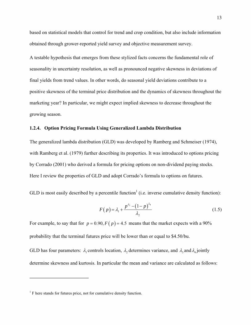
1.2.4. Option Pricing Formula Using Generalized Lambda Distribution
The generalized lambda distribution (GLD) was developed by Ramberg and Schmeiser (1974),
with Ramberg et al. (1979) further describing its properties. It was introduced to options pricing
by Corrado (2001) who derived a formula for pricing options on non-dividend paying stocks.
Here I review the properties of GLD and adopt Corrado’s formula to options on futures.
GLD is most easily described by a percentile function1 (i.e. inverse cumulative density function):
43
12
1p pF p
(1.5)
For example, to say that for 0.90, 4.5p F p means that the market expects with a 90%
probability that the terminal futures price will be lower than or equal to $4.50/bu.
GLD has four parameters: 1 controls location, 2 determines variance, and 3 and 4 jointly
determine skewness and kurtosis. In particular the mean and variance are calculated as follows:
1 F here stands for futures price, not for cumulative density function.

14
1 2
2 2 22
/
/
A
B A
(1.6)
with3 4
1 1
1 1A
and 3 4
3 4
1 12 1 ,1 2
1 2 1 2B
,where
stands for the
complete beta function. Ramberg et al. give expressions for the third and fourth central moments
of the distribution:
33
3 32
2 44
4 42
3 2
4 6 3
C AB AE x
D AC A B AE x
The skewness and kurtosis formulas are:
3 33
3 3/23 3 3 22
2 4 2 44
4 24 4 4 22
3 2 3 2
4 6 3 4 6 3
C AB A C AB A
B A
D AC A B A D AC A B A
B A
(1.7)
where expressions for C and D are:
3 4 3 43 3
1 13 1 2 ,1 3 1 ,1 2
1 3 1 3C
3 4 3 4 3 43 3
1 14 1 3 ,1 4 1 ,1 3 6 1 2 ,1 2
1 4 1 4D
We see that the 3 and 4 parameters influence both location and variance, however 1 influences
only the first moment, and 2 influences only the first two moments. Thus, skewness and kurtosis
do not depend on 1 and 2 .
A standardized GLD has a zero mean and unit variance, and has a percentile function of the
form:

15
43
3 4 4 3
1 1 11
, 1 1F p p p
h
(1.8)
with 22 3 4 3,h sign B A and 1 3 4
4 3
1 1/ ,
1 1h
.
From here, we can move more easily to an options pricing environment. We wish to make GLD
an approximate generalization of the log-normal distribution so I keep the mean and the variance
the same as in (1.4), while allowing skewness and kurtosis to be separately determined by the 3
and 4 parameters. Therefore, the percentile function relevant for option pricing will be
2
430
3 4 4 3
1 1 11 1
, 1 1
teF p F p p
h
(1.9)
Note that this is equivalent to (1.5) with
2
1 03 4 4 3
1 1 1
, 1 1
teF
h
and
2
3 42
,
1t
h
e
. This will guarantee that the first two moments of the terminal distribution
will be 22 20 0 1tF F e , just as in Black’s model.
The pricing formula for European calls is
0 3 4 0, , , , , , , 0rT
TV K F T r e Max F K dp F (1.10)
As shown by Corrado (2001), I can simplify this through a change-of-variable approach where
TF p F :
1
0, 0T TK p K
Max F K dp F F K dp F F p K dp
(1.11)
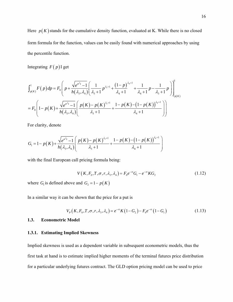
16
Here p K stands for the cumulative density function, evaluated at K. While there is no closed
form formula for the function, values can be easily found with numerical approaches by using
the percentile function.
Integrating F p I get
2 4
3
2 43
11
1 10
3 4 3 4 4 3
11
03 4 3 4
11 1 1 1
, 1 1 1 1
1 111
, 1 1
t
p K
p K
t
peF p dp F p p p p
h
p K p Kp K p KeF p K
h
For clarity, denote
2 43
11
13 4 3 4
1 111
, 1 1
t p K p Kp K p KeG p K
h
with the final European call pricing formula being:
0 3 4 0 1 2, , , , , , rt rtV K F T r F e G e KG (1.12)
where 1G is defined above and 2 1G p K
In a similar way it can be shown that the price for a put is
0 3 4 2 0 1, , , , , , 1 1rt rtPV K F T r e K G F e G (1.13)
1.3. Econometric Model
1.3.1. Estimating Implied Skewness
Implied skewness is used as a dependent variable in subsequent econometric models, thus the
first task at hand is to estimate implied higher moments of the terminal futures price distribution
for a particular underlying futures contract. The GLD option pricing model can be used to price
17
only European options, that is, options that can only be exercised at contract maturity. As
mentioned before, options on corn futures are American options, i.e. they can be also exercised
at any time before contract maturity. Therefore, for each option trade I use in fitting implied
GLD higher moments, I first need to calculate the price at which such an option would trade if it
indeed were of the European type. To do this, for each data point, I separately estimate implied
volatility using CRR binomial trees with 500 steps. Then, for each observation separately, I use
Black’s model to calculate the price of a European option with same futures price, strike, interest
rate and time to maturity as that record for actually traded American option.
Using calibrated premiums for European options on corn futures, I then fit the following option
pricing model to options of a particular contract month:
0 3 4, , , , , ,Ei i i iO V K F r (1.14)
where function used is as in (1.12) for calls or (1.13) for puts, EiO would be the previously
calibrated option premium for trade i for an option with strike iK and with 0iF being the last
observed traded futures price prior to this trade. Observed parameters common to all options of
the same contract month traded on the same day include the interest rate r and the time to
maturity measured in calendar days, denoted as .
The unobserved generalized lambda distribution parameters 3 4, , jointly determine variance,
skewness and kurtosis of the implied terminal distribution of futures prices, and are assumed to
be the same for all trades occurring on a single trading day. Implied parameters are fitted by a
nonlinear least squares model, minimizing squared differences between calibrated option
premiums for European options, and option premiums that arise from the GLD option pricing

18
model. Models are estimated separately for each trading day and each contract month traded at
that day.
1.3.2. Modeling Intra-year Dynamics of Implied Skewness
As I postulated in section 1.2.3, corn physiology in conjunction with weather patterns should
play a major role in governing the intra-year dynamics of implied skewness. The panels in
Figure 1.8 present scatter diagrams of estimated implied skewness over the life of particular
contract months. Each dot represents the estimated implied skewness on a particular trading day,
with bolded diamonds being averages for a particular time-to-maturity horizon over the 15
marketing years used in estimation (1995-2009). Visual inspection does not contradict patterns I
expected to see. In particular, new-crop contracts (September and December), exhibit near flat
average implied skewness until late June, followed by a concave decrease for the September
contract, and linear downward trend for December. Patterns for carry contracts (March, May and
July) share strong and concave decreases in implied skewness over the last four months of
contract life, with the effects on implied skewness during corn growth period not as distinct as
for new-crop contracts. All five patterns stand in stark contrast to Black’s model where variance
of the terminal futures price distribution is assumed to be decreasing linearly in time. Given that
Black’s model stipulates the terminal distribution to be lognormal, a linear decrease in variance
would correspond to a slightly convex and smooth decline in implied skewness.
If skewness in options on corn futures arises due to asymmetry in the ability of old-crop stocks to
mitigate price effects of unexpected weather events during the growing season then skewness
should exhibit different dynamics before corn silking, during the growing season, and post-
harvest. To test this hypothesis, I fit implied skewness as a function of time using several

19
models. Let implied skewness be denoted with tIS . If options expire at time T , then the
remaining time to maturity T t is denoted as . The models I test can then be written as
Linear model:
1t tIS (1.15)
Quadratic model:
21 2t tIS (1.16)
Linear model with one change in regime (timing is estimated endogenously):
1 1 1 2 2 1
1 1 1 2 2 1. . t tIS
s t
(1.17)
Quadratic model with one change in regime (timing is estimated endogenously):
2 2
1 1 1 1 2 2 2 1
2 21 1 1 1 1 2 2 1 1. .
t tIS
s t
(1.18)
Quadratic model with two changes in regime (timing is estimated endogenously):
2 2 21 1 1 1 2 2 2 2 1 3 3 3 2
2 21 1 1 1 1 2 2 1 2 1
2 22 2 2 2 2 3 3 2 3 2
. .
t tIS
s t
(1.19)
Simple linear (1.15) and quadratic models (1.16) are used as benchmarks. In particular, it is
interesting to compare the performance of model (1.16) to more complicated models as model
(1.16) together with a restriction that 2 be positive (i.e. IS exhibiting a convex pattern over
time) follows as an implication of Black’s option pricing model. Different skewness dynamics
through a marketing year would be captured either by estimating higher polynomial or multiple-
regime models. In the multiple-regime models fit here, the restrictions listed above result in
20
continuity of predicted implied skewness at points of regime change, but smoothness at those
points is not imposed.
The points at which regimes changes, i.e. 1 in models (1.17) and (1.18) and 1 2, in model
(1.19) are also treated as parameters that need to be estimated, rather than being pre-determined.
Conditional on a particular choice of these parameters, the rest of the model can be estimated
using restricted least squares. For one-switch models, similar to Hansen (1999), denote the sum
of square errors for restricted least squares estimates conditional on a particular value of 1 as
1SSE . The optimal point for the regime switching time is found as the minimizer of the
conditional restricted sum of square errors:
1 arg min SSE
(1.20)
For models with two switches, I can find the optimal switching points through a three-step
minimization. First, conditional on particular values of 1 2, I can find the optimal slope
coefficients by restricted least squares estimation. Then, like above
2 1
1 1
2 1 1 2
1 1 2 1
| arg min ,
arg min , |
SSE
SSE
(1.21)
where 1 1 1: 20 50MAX and 2 1 2 1 2: 30 20 .
To implement this when estimating optimal points for regime switching, conditional on
stipulating the number of regime switch points, simple grid search is used, and then the sum of
squared errors (SSE) from the estimated restricted least squares are ranked. I stipulate that
regime switching cannot be less than 20 days to expiry or closer than 20 days to the maximum
time to maturity. For models with two switch dates, I also stipulate that the two switch dates
cannot be less than 30 days apart. The model with the lowest SSE is chosen as best in its class.
21
Models are estimated separately for each contract month (March, May, July, September and
December), using daily values of implied skewness for the period 1995-2009. To repeat, implied
skewness is itself estimated using high-frequency data as described in the previous section. As
such, implied skewness estimates become very unstable on a day-to-day basis for very high time
to maturity horizons. One reason could be a lack of liquidity in options markets for options far
from expiry, and another the low number of years for which options with such long horizons
have even been traded. To eliminate the effect of noise in the estimation of implied skewness for
long time to maturity horizons, I truncate the maximum allowable time to maturity for each
contract separately at the point where simple visual inspection indicates noise starts to dominate.
In selecting the optimal model specification among the five models listed, I have used the theory
developed by Hansen (1996, 1999, 2000) and used in Cox, Hansen and Jimenez (2004). As
Hansen (1996) explains, the problems of inference in the presence of nuisance parameters (i.e.
regime switching times) is that they are not identified under the null hypothesis of no-regime
change. If I fixed the regime switching-time to a particular value, I could perform a standard
Wald test to see if parameters for intercept and slopes are equal for observations occurring before
and after days to maturity. However, since I cannot restrict the possible threshold time a priori,
as Hansen (1996) explains, the asymptotic distribution of standard tests are nonstandard and
nonsimilar, which means that tabulation of critical values is impossible. The finite sample
distribution of the Wald statistic under the null hypothesis is calculated by simulation and the
null hypothesis is rejected if the test statistic is higher than the desired percentile of the simulated
Wald statistic distribution under the null. Details of the bootstrapping method used in testing for
the optimal model class are presented in section 1.3.2.

22
1.3.3. Inter-year Variation of Implied Skewness
Finally, I turn to explaining the inter-year variations in implied skewness. As argued in the
previous section, skewness will likely be impacted by weather once corn silking starts.
Therefore, if we are to infer an impact of storage on skewness across many years, each with its
own weather peculiarities, we should choose the time before the reproductive growth phase
starts, i.e. no later than third week of June. If we were to choose skewness observed much earlier
than that, we would risk falling in the endogeneity trap. Before a marketing year is close to the
end, consumption can react to changes in futures price, possibly even to changes in options
premiums, thus increasing or decreasing carryout stocks. It would make little sense then to use
expected ending stocks-to-use as a predetermined explanatory variable and implied skewness as
a dependent variable. To avoid this problem, the expected ending stocks-to-use ratio of the
previous marketing year, as reported in June edition of World Agricultural Supply and Demand
Estimates (WASDE) report2 is employed for explanatory variable for storage adequacy.
If the price elasticity of supply for corn is not zero, we would expect producers to react to tighter
expected stocks and higher new crop prices with an increase in planted acreage, so acreage
response is the second variable I need to include in the model. Specifically, I use the measure of
change between intended plantings for a given year as reported in the USDA Prospective
2 WASDE is produced by World Agricultural Outlook Board, inter-agency body at United States Department of Agriculture. Historical WASDE reports can be accessed at http://usda.mannlib.cornell.edu/MannUsda/viewDocumentInfo.do?documentID=1194

23
Plantings3 report published at the end of March, and the actual acreage planted in the previous
marketing year.
In addition to supply side covariates, I need to address possible asymmetries in uncertainty of
demand. Domestically, corn is used as a livestock feed, an industrial sweetener and as an input in
ethanol production. All three of these derived demand categories are likely impacted by
macroeconomic shocks. Therefore, as a measure of demand uncertainty I use the June-to-June
change in the national unemployment rate as published by the Bureau of Labor Statistics.
The final econometric model has the following form:
1 2 3/t t T t T t tIS E A E S D U (1.22)
Where tIS stands for implied skewness for a December contract of year t estimated as the
average of implied skewness for the 10 trading days following the June WASDE report. The
change in acreage planted is TA . Since in June I only observe intended plantings, this is written
as the expected change in acreage. Expected ending stocks-to-use is /t T tE S D and tU is the
June-to-June change in the U.S. unemployment rate. Theory predicts that all coefficients except
the constant should be negative. A stronger acreage response and higher carryout stocks relative
to demand imply more ability to buffer adverse weather shocks, and will thus reduce skewness.
Likewise, a more unstable macroeconomic environment will decrease demand for fuel and
possibly even for meat, thus reducing upward pressure on corn prices.
3 Prospective Plantings is a government report produced annually by the National Agricultural Statistics Service, an agency of the United States Department of Agriculture. Historical Prospective Plantings reports can be accessed at http://usda.mannlib.cornell.edu/MannUsda/viewDocumentInfo.do?documentID=1136
24
1.4. Data
Commodity futures for corn as well as options on futures are traded on the Chicago Mercantile
Exchange (formerly the Chicago Board of Trade). A dataset comprising all recorded
transactions, i.e. times and sales data (also known as “tick data”) for both futures and options on
futures, for the period 1995 through 2009, was obtained. It includes data for both the regular and
electronic trading sessions. The total number of transactions exceeds 30 million, including 22
million observations on futures contract trades, and about 10 million trades in options contracts.
Options data were matched with the last preceding futures transaction. LIBOR interest rates were
obtained from British Bankers’ Association, and represent the risk-free rate of return. Overnight,
1 and 2 weeks, and 1 through 12 months of maturity LIBOR rates for period the 1995 through
2009 were used to obtain the arbitrage-free option pricing formulas. In particular, each options
transaction was assigned the weighted average of interest rates with maturities closest to the
contract traded. To avoid serial correlation in residuals from estimating implied coefficients, the
data frequency was reduced to not less than 15 minutes between transactions for the same
options contract. This resulted in data sets of between 200 to 800 recorded transactions for a
particular trading day for a total of around 1.1 million observations used in estimation. For each
data point I separately estimate implied volatility using CRR binomial trees with 500 steps.
Then, for each data point, the price of a European option using Black’s formula is calculated
using the same parameters (futures price, interest rate, time to maturity) as that recorded for the
American option. In addition, volatility is set equal to the one implied for American options.
These ‘artificial’ European options are then used in fitting parameters of GLD option pricing
model for each trading day separately.

25
As stated in the previous section, the implied skewness used in the econometric analysis is
calculated as a simple average over 10 business days following the June WASDE report. Due to
the high incidence of limit-move days and days with high intraday price changes the year 2008 is
excluded from the sample. Including 2008 would render the calculation of higher moments
unreliable. Descriptive statistics of the variables used in econometric analysis are given in
Table 1.1, and corn supply/demand balance sheets are in Table 1.2.
Figure 1.9 presents a scatter diagram of expected ending stocks-to-use vs. implied skewness.
Note the inverse relationship between these variables and the beneficial impact of the acreage
response. For example, in the summer of 1996, carryout stocks-to-use were only 4.03%, two
standard deviations below the average for 1995-2009. However, skewness was below the mean,
due to a 12.2% increase in expected acreage, which is 2.2 standard deviations above the average
increase of 1.4%. Similarly, in 2007 carryout stocks were only 8.56% of demand, but a massive
acreage increase of 15.5%, by far the largest in this sample, reduced the skewness below the
mean. It is instructive to look at 2006 as well. Although ending stocks were bountiful at 19.67%
of demand, a reduction in acreage of 4.6% made for the third largest skewness in the sample.
1.5. Estimation Procedure and Results
1.5.1. Estimating Parameters of GLD Distribution and Implied Higher Moments
As stated in section 1.3.1, for each contract, for each trading day, I separately estimate the
parameters 3 4, ,and in the GLD option pricing formula. In particular, I minimize the squared
difference in option premiums calculated with the GLD formula, and prices of European options
as implied by Black’s model. To do so, I first need a starting value for the implied volatility of an
option with a strike price closest to the underlying futures price. The starting values for the 3
26
and 4 parameters were chosen to correspond to the skewness and kurtosis of the terminal futures
price as they would be under the restriction that the logarithm of the terminal price is normally
distributed with variance equal to 2t , where 2 is the square of the starting value for the
implied sigma parameter. Excel Solver is used to run the minimization problem, utilizing a
FORTRAN compiled library (.dll file) created by Corrado (2001) that estimates GLD European
Call prices. A formula for the GLD European put option was then programmed in Visual Basic
for Applications.
Estimated lambda parameters are employed to calculate implied skewness and kurtosis. GLD
option prices seem to work rather well, with an average absolute pricing error about 3/8 of a cent
per bushel, and a maximum pricing error usually reaching not more than 2 cents (this occurs for
the least liquid and most away from the money options). While there may be issues regarding the
robustness of implied parameters with respect to starting values, the implied parameters seem to
be rather stable from one day to the next. For December 2007 corn, for example, the skewness
estimated between June 11 and June 25, 2007 varies between 1.15 and 1.26. For that year, the
average absolute pricing error was 7/8 of a cent per bushel, with a maximum pricing error of 7.9
cents.
For all years in the sample, the implied skewness is 1.2 to 3 times higher than it would be if the
logarithm of the terminal futures price was really expected to be normal. Implied kurtosis is 1.2
to 1.6 times higher than that predicted by Black’s model. I thus see that deviations from Black’s
model are particularly pronounced in implied skewness.

27
1.5.2. Dynamics of Intra-year Implied Skewness: Results
The results of intra-year models for dynamics of implied skewness are presented in Table 1.3,
and predicted implied skewness for each contract month is plotted in Figure 1.10. For all five
contracts, the quadratic model improves fit dramatically over the linear model. To perform a
formal test whether a model with one switching time and quadratic segments fits the data better
than the quadratic model, I have used the bootstrapping procedure described by Cox, Hansen and
Jimenez (2004). In doing this test, I shall refer to the quadratic model (1.16) as the restricted
model and model (1.18) as the unrestricted model. These models are nested, i.e. model (1.16) is
obtained by imposing restrictions 1 2 1 2 1 2, , . Under the null hypothesis that these
restrictions hold the switching time 1 is not identified. To test the null hypothesis, I first make
2000 bootstrap samples using the fixed-regressors residual bootstrapping method. In particular,
for each simulation values of implied skewness are calculated by adding a draw from the
empirical distribution of residuals to predicted value of the dependent variable. Fitting is done
using the estimated coefficients from the restricted model, in this case model (1.16). Then, for
each bootstrapped sample, parameters of the unrestricted model, including switching time, are
calculated by the same method as before, i.e. combining a grid search and concentrated restricted
least squares. A Wald statistic 0 1
1n
SSE SSEW n
SSE
is then calculated for that particular
replication, where n is the number of observations in the sample, 0SSE is the sum of square
errors in the restricted model (zero switching points) using bootstrapped data and 1SSE is the sum
of square errors of model (1.18) using bootstrapped data. The entire process is repeated 2000
times to obtain a finite sample distribution of the Wald statistic. The null hypothesis is rejected if
the Wald statistic obtained using the original data is higher than the 95th percentile of the

28
simulated distribution. We see from Table 1.3 that model (1.16) is strongly rejected in favor of
model (1.18) for all five contract months.
I also estimate a model with two regimes changes. For the May contract, the optimal first
switching time solves to a corner solution, i.e. 20 days less than the maximum time-to-maturity
used in estimation. I interpret this as evidence that for the May contract, a model with two
regime switching times does not explain the data any better than models with one change in
regime, and is in fact a misspecification, i.e. number of break points is stipulated to be higher
than actually exist. For other contract months, the optimal switching time solves out to the
interior of the allowable set of times, and I need to perform a formal test to investigate if models
with two switching times are indeed better representations of the data. Bootstrapping is again
employed. In particular, the null hypothesis now is that true model is model (1.18), and the
unrestricted model is model (1.19). Model (1.18) can be obtained from model (1.19) by
restricting it, such that coefficients satisfy: 1 2 1 2 1 2, , .
I again use fixed-regressors residual-bootstrap technique and add draws from the empirical
distribution of residuals obtained from model (1.18) to the implied skewness measures predicted
using the estimated coefficients of model (1.18). For each replication, a Wald statistic
1 2
2n
SSE SSEW n
SSE
is calculated, where 1SSE is the sum of square errors obtained by
estimating model (1.18) on bootstrapped data, and 2SSE is calculated by estimating the model
with two switching times on bootstrapped data. As before, the entire process is repeated 2000
times to obtain a finite sample distribution of the Wald statistic. The null hypothesis is rejected if
the Wald statistic obtained using original data is higher than the 95th percentile of the simulated
distribution. I find that the Wald statistics obtained using the original data are low enough that

29
the null hypothesis cannot be rejected for any contract month, and p-values are exceptionally
large. In conclusion, statistical tests show that a model with 1 regime change is superior. To test
if model (1.18) explains the data any better than model (1.17) with two linear segments I can use
standard critical values in Wald test, as both models have the same number of regimes. I find that
the null is rejected for all contract months.
The next issue to investigate and explain concerns evaluated knot times and their confidence
intervals. Point estimates are found using the already explained estimation procedure. Residual-
based bootstrap is then used to obtain confidence intervals. For a particular contract month,
simulated data is created by adding draws from the empirical distribution of residuals to the
predicted implied skewness using the same model for which I evaluate confidence intervals of
the knot. The model is then re-estimated on simulated data, and a new optimal knot value is
noted. The procedure is repeated 2000 times, with the confidence interval obtained using the
2.5th and 97.5th quantile as the lower and upper bounds, respectively. For model (1.18) with
quadratic segments, I find that the confidence intervals for switching times are substantial for
May and July contracts. A possible reason is that the first segment in the model is convex, and
the second concave, creating a rather smooth transition. In such a setting, changing the knot
value can be very easily compensated for by changes in the slopes parameters. For the
September, December and March contracts, both segments are estimated with concave curves,
and exhibit much tighter confidence intervals of the switching times. Results are presented in
Table 1.3. As a robustness check, I also calculate asymptotic confidence intervals using a method
developed by Hansen (2000) that involves inverting a likelihood ratio statistic. I find that our
bootstrapping method matches closely the results obtained using asymptotics for all contract
months except July. For that contract month, the curve for the likelihood ratio statistic is rather
30
flat and close to the asymptotic critical value for time-to-maturity values included in the
bootstrapped confidence interval. In that sense, we perhaps could say that the bootstrap produces
more conservative estimates for the confidence intervals. Another likely reason for observed
differences could be that I estimate our model with the additional restriction of continuity in
predicted variable, whereas asymptotic distribution is developed for unrestricted least squares
estimation.
In the model with 1 regime change and quadratic segments, optimal switching time for
September contract is 69 days to maturity, and for December it is 160 days. It will help us to be
able to map time-to-maturity measures to a particular date in a year. Option contract
specifications state that last trading day is “The last Friday preceding the first notice day of the
corresponding corn futures contract month by at least two business days.” The first notice day is
the first day of the delivery month. For simplicity, I approximate the last option trading day to be
25th of the month preceding the delivery month. Under such an approximation, regime switching
times for new-crop contracts correspond to June 18th for the September contract and June 19th for
the December contract. To test if regime switching times for these two contracts really fall on the
same calendar date, I perform a Wald test. This is a non-standard test and I use residual-based
bootstrapping to generate data under the null hypothesis that calendar switching dates are the
same, which is equivalent to restriction that 90.DEC SEP The null hypothesis is not
rejected, and p-value is 0.9995, with the original Wald statistic is higher than only one out of
2000 Wald statistics simulated under the null hypothesis. The Crop progress report4 published in
4 Crop Progress report is a government report produced weekly from April through November of each year by the National Agricultural Statistics Service, an agency of the United States Department of Agriculture. Historical Prospective Plantings reports can be accessed at http://usda.mannlib.cornell.edu/MannUsda/viewDocumentInfo.do?documentID=1048

31
last week of June is normally the first such report to list corn silking progress. These reports
suggest that on average about 5% of the U.S. corn crop is silking by June 26th. Thus, dynamics
of implied skewness for new-crop contracts appear to change right at the start of the corn silking
period.
For carry contracts I find quite a different dynamic. Regime changes for the March, May and
July contracts occur respectively at 130, 125 and 112 days to maturity. Suspecting that these
days account for similar patterns across contracts, I tested whether regime changes occur at
statistically significantly different time-to-maturity horizons. Similar to a previous hypothesis
test, I express that hypothesis as restrictions on switching times: MAR MAY JUN . The optimal
switching time under the null hypothesis (that the restriction holds) is 128 days to maturity, and
the null is not rejected. This common switch is manifested in Figure 1.8 as concave and
substantial decrease in implied skewness close to contract expiry. This likely reflects the decline
in overall uncertainty concerning terminal prices as maturity approaches. It is more interesting to
note that for carry contracts, the first segment (i.e. before the switch) is convex for the May and
July contracts, but concave for March. This could reflect that fact that for March contract, corn
growth-sensitive period falls in the middle of the March contract lifetime, while for May and
July this growth period is at the beginning of the contract life.
Table 1.4 showcases the relative contribution of the corn growth period (silking through harvest,
approximated by the dates June 20 to October 20) to skewness reduction during a contract’s
lifetime. For carry contracts the days spent in second regime at the end of the contract life are
excluded. For example, for the July contract, the maximum time to maturity was 350 calendar
days. The contract traded for 230 calendar days prior to entering the “finish-line” period, i.e. the
last 120 days in which I find a strong reduction of skewness. Out of those 230 days, 113 days, or
32
49.1% of time, falls in the growth sensitive period. At the maximum time-to-maturity horizon
predicted implied skewness is 1.419, and at switch time it is 1.218. Although the growth
sensitive period constitutes only one half of that time, it accounts for 76.5% of the difference
between the maximum time-to-maturity horizon and switch time implied skewness. For the
March contract, I see a situation that is even more extreme – the sensitive growth period
constitutes 59.5% of the pre-switch life, but accounts for 94.3% of the difference between
skewness at maximum time-to-maturity and at the switch-time.
1.5.3. Intra-year Variation in Implied Skewness: Results
Results of the previous section further justify using implied skewness for December contract
over 10 days after June WASDE report in investigating effect of expected stocks-to-use at the
end of a marketing year (Aug. 31) on implied skewness. To test this, a simple linear regression is
estimated for the period 1995-2009 using implied skewness as the dependent variable. The
independent variables include a constant, the expected ending stocks-to-use, the expected
planned change in planted acreage and changes in the unemployment rate. Regression statistics
are reported in Table 1.5. Due to very low degrees of freedom (10), I have to rely on t-table for
critical values, and use a one-tail test for the stocks-to-use coefficient.
An 1 % increase in stocks-to-use reduces skewness by 0.015. This coefficient is statistically
significant at the 95% confidence level. To put this number in perspective, the difference
between the lowest and the highest ending stocks-to-use recorded in the sample reduces
skewness from 1.47 to 1.24, which is 47% of the difference between the highest and the lowest
recorded skewness in the sample. Coefficients for demand uncertainty and acreage response are
also statistically significant and have the expected sign.
33
1.6. Conclusions and Further Research
An option pricing model based on a generalized lambda distribution provides a useful heuristic
in thinking about determinants of the shape of terminal futures price conditional distributions.
Results indicate that crop inventories and plant physiology play a significant role in determining
the expected asymmetry of the terminal distribution. In particular, results reveal that implied
skewness is much more persistent than implied by Black’s model. In years with low implied
volatility implied skewness remains much higher than would be the case under the lognormality
restriction, and dynamics are dominated not by time to maturity, but by temporal patterns in the
resolution of uncertainty regarding crop yields.
Further research will focus on extending this analysis to soybeans and wheat. The U.S. is a major
world player in corn, with 55.6% of world exports. That is higher than 45.3% of world exports of
soybeans, and much higher than 17.7% percent in wheat. Extending the analysis to other crops
will identify the effect of trade and non-overlapping growing seasons in different countries on
the magnitude, inter-year differences and intra-year dynamics on implied higher moments of the
terminal price distribution.
Thus far the literature has focused on evaluating the impacts of government reports on implied
volatility coefficients. The model presented here allows us to extend this to higher moments and
examine how reports (i.e., information) influence the entire distribution of prices, not just the
second moment. For example, I could use weekly crop progress reports to explain inter-year
differences in the evolution of skewness through the summer months.
In the absence of high frequency data, many researchers use end of day reported prices for
futures and options to evaluate implied higher moments. By re-estimating this model using only

34
end of day data it is possible to examine the amount of noise and possible direction of bias such
an approach brings to estimates of implied higher moments.
What happens when storage is not available to partially absorb the shocks to supply? It would be
interesting to use the GLD option pricing model to examine the evolution and determinants of
higher moments of non-storable commodities. Further research is needed to examine the impact
of durability of production factors for commodities that are themselves not storable.
Finally, impacts of market liquidity and trader composition on the levels and stability of implied
higher moments is a promising new area for research. With careful design of the analysis, we
may be able to find a way to separate the part of the option price that is due to implied terminal
price distributions from additional premium influences incurred due to hedging pressure or lack
of market liquidity.
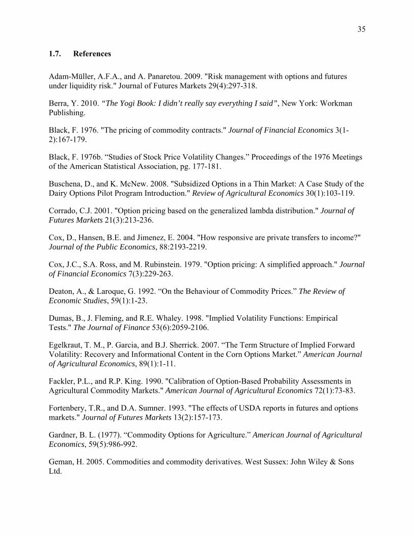
35
1.7. References
Adam-Müller, A.F.A., and A. Panaretou. 2009. "Risk management with options and futures under liquidity risk." Journal of Futures Markets 29(4):297-318.
Berra, Y. 2010. “The Yogi Book: I didn’t really say everything I said”, New York: Workman Publishing.
Black, F. 1976. "The pricing of commodity contracts." Journal of Financial Economics 3(1-2):167-179.
Black, F. 1976b. “Studies of Stock Price Volatility Changes.” Proceedings of the 1976 Meetings of the American Statistical Association, pg. 177-181.
Buschena, D., and K. McNew. 2008. "Subsidized Options in a Thin Market: A Case Study of the Dairy Options Pilot Program Introduction." Review of Agricultural Economics 30(1):103-119.
Corrado, C.J. 2001. "Option pricing based on the generalized lambda distribution." Journal of Futures Markets 21(3):213-236.
Cox, D., Hansen, B.E. and Jimenez, E. 2004. "How responsive are private transfers to income?" Journal of the Public Economics, 88:2193-2219.
Cox, J.C., S.A. Ross, and M. Rubinstein. 1979. "Option pricing: A simplified approach." Journal of Financial Economics 7(3):229-263.
Deaton, A., & Laroque, G. 1992. “On the Behaviour of Commodity Prices.” The Review of Economic Studies, 59(1):1-23.
Dumas, B., J. Fleming, and R.E. Whaley. 1998. "Implied Volatility Functions: Empirical Tests." The Journal of Finance 53(6):2059-2106.
Egelkraut, T. M., P. Garcia, and B.J. Sherrick. 2007. “The Term Structure of Implied Forward Volatility: Recovery and Informational Content in the Corn Options Market.” American Journal of Agricultural Economics, 89(1):1-11.
Fackler, P.L., and R.P. King. 1990. "Calibration of Option-Based Probability Assessments in Agricultural Commodity Markets." American Journal of Agricultural Economics 72(1):73-83.
Fortenbery, T.R., and D.A. Sumner. 1993. "The effects of USDA reports in futures and options markets." Journal of Futures Markets 13(2):157-173.
Gardner, B. L. (1977). “Commodity Options for Agriculture.” American Journal of Agricultural Economics, 59(5):986-992.
Geman, H. 2005. Commodities and commodity derivatives. West Sussex: John Wiley & Sons Ltd.
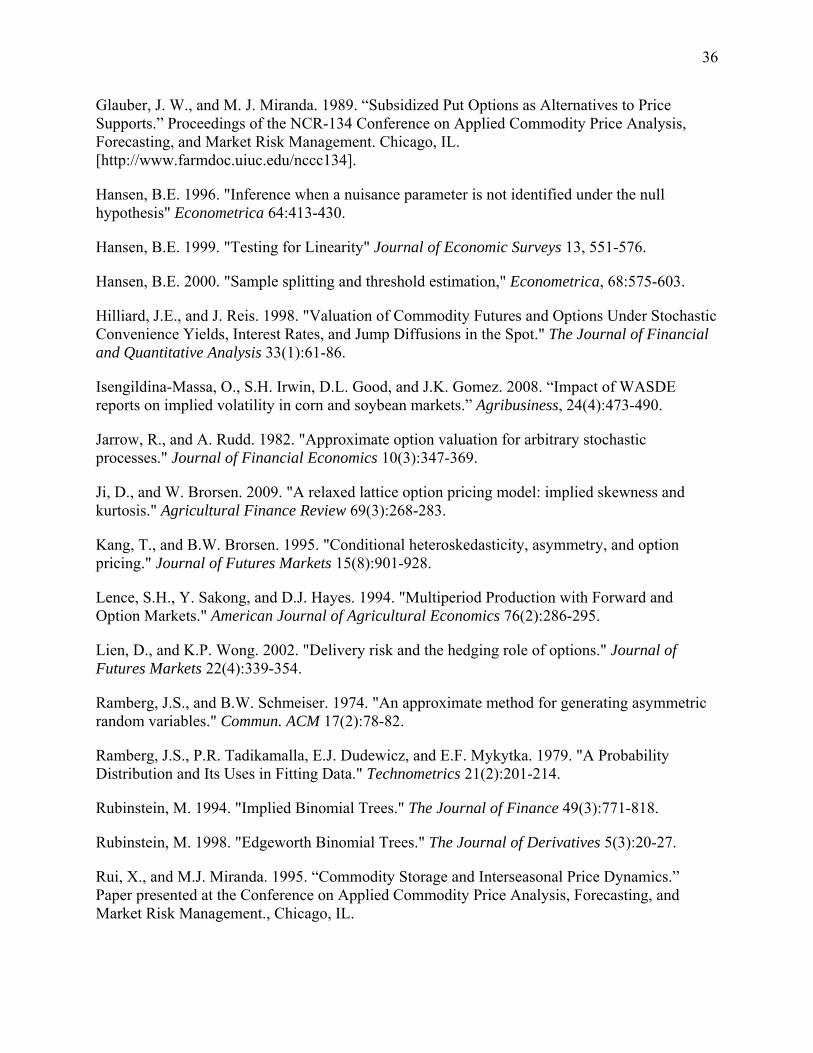
36
Glauber, J. W., and M. J. Miranda. 1989. “Subsidized Put Options as Alternatives to Price Supports.” Proceedings of the NCR-134 Conference on Applied Commodity Price Analysis, Forecasting, and Market Risk Management. Chicago, IL. [http://www.farmdoc.uiuc.edu/nccc134].
Hansen, B.E. 1996. "Inference when a nuisance parameter is not identified under the null hypothesis" Econometrica 64:413-430.
Hansen, B.E. 1999. "Testing for Linearity" Journal of Economic Surveys 13, 551-576.
Hansen, B.E. 2000. "Sample splitting and threshold estimation," Econometrica, 68:575-603.
Hilliard, J.E., and J. Reis. 1998. "Valuation of Commodity Futures and Options Under Stochastic Convenience Yields, Interest Rates, and Jump Diffusions in the Spot." The Journal of Financial and Quantitative Analysis 33(1):61-86.
Isengildina-Massa, O., S.H. Irwin, D.L. Good, and J.K. Gomez. 2008. “Impact of WASDE reports on implied volatility in corn and soybean markets.” Agribusiness, 24(4):473-490.
Jarrow, R., and A. Rudd. 1982. "Approximate option valuation for arbitrary stochastic processes." Journal of Financial Economics 10(3):347-369.
Ji, D., and W. Brorsen. 2009. "A relaxed lattice option pricing model: implied skewness and kurtosis." Agricultural Finance Review 69(3):268-283.
Kang, T., and B.W. Brorsen. 1995. "Conditional heteroskedasticity, asymmetry, and option pricing." Journal of Futures Markets 15(8):901-928.
Lence, S.H., Y. Sakong, and D.J. Hayes. 1994. "Multiperiod Production with Forward and Option Markets." American Journal of Agricultural Economics 76(2):286-295.
Lien, D., and K.P. Wong. 2002. "Delivery risk and the hedging role of options." Journal of Futures Markets 22(4):339-354.
Ramberg, J.S., and B.W. Schmeiser. 1974. "An approximate method for generating asymmetric random variables." Commun. ACM 17(2):78-82.
Ramberg, J.S., P.R. Tadikamalla, E.J. Dudewicz, and E.F. Mykytka. 1979. "A Probability Distribution and Its Uses in Fitting Data." Technometrics 21(2):201-214.
Rubinstein, M. 1994. "Implied Binomial Trees." The Journal of Finance 49(3):771-818.
Rubinstein, M. 1998. "Edgeworth Binomial Trees." The Journal of Derivatives 5(3):20-27.
Rui, X., and M.J. Miranda. 1995. “Commodity Storage and Interseasonal Price Dynamics.” Paper presented at the Conference on Applied Commodity Price Analysis, Forecasting, and Market Risk Management., Chicago, IL.

37
Shaw, R. H., J. E. Newman, D. G. Baker, R. V. Crow, R. F. Dale, Rich Feltes et al. 1988. "Weather Stress in the Corn Crop." OSU current report - Oklahoma State University, Cooperative Extension Service, Vol. 2099.
Sherrick, B.J., P. Garcia, and V. Tirupattur. 1996. "Recovering probabilistic information from option markets: Tests of distributional assumptions." Journal of Futures Markets 16(5):545-560.
Thomsen, M.R., A. McKenzie, and G.J. Power. 2009. "Volatility Surface and Skewness in Live Cattle Futures Price Distributions with Application to North American BSE Announcements." Paper presented at 2009 AAEA & ACCI Joint Annual Meeting. Milwaukee, WI.
World Agricultural Outlook Board. 2010. “World Agricultural Supply and Demand Estimates.” United States Department of Agriculture. Retrieved October 4, 2010 from http://usda.mannlib.cornell.edu/MannUsda/viewDocumentInfo.do?documentID=1194
National Agricultural Statistics Service. 2010. “Prospective Plantings.” United States Department of Agriculture. Retrieved October 4, 2010 from http://usda.mannlib.cornell.edu/MannUsda/viewDocumentInfo.do?documentID=1194
Vercammen, J. 1995. "Hedging with Commodity Options When Price Distributions Are Skewed." American Journal of Agricultural Economics 77(4):935-945.
Williams, J.C., and B. Wright. 1991. Storage and commodity markets. Cambridge ; New York: Cambridge University Press.
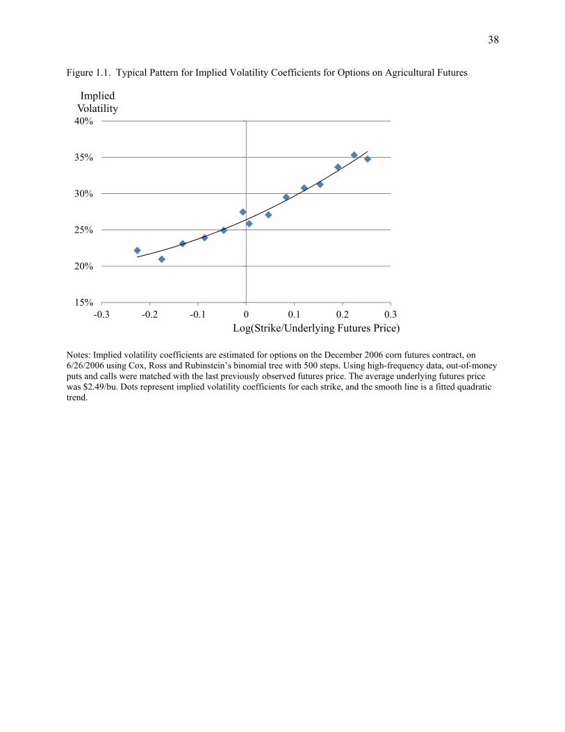
38
Figure 1.1. Typical Pattern for Implied Volatility Coefficients for Options on Agricultural Futures
Notes: Implied volatility coefficients are estimated for options on the December 2006 corn futures contract, on 6/26/2006 using Cox, Ross and Rubinstein’s binomial tree with 500 steps. Using high-frequency data, out-of-money puts and calls were matched with the last previously observed futures price. The average underlying futures price was $2.49/bu. Dots represent implied volatility coefficients for each strike, and the smooth line is a fitted quadratic trend.
15%
20%
25%
30%
35%
40%
-0.3 -0.2 -0.1 0 0.1 0.2 0.3
Implied Volatility
Log(Strike/Underlying Futures Price)

39
Figure 1.2. Evolution of Implied Volatility Curve for Options on Dec’ 04 and Dec ’06 Corn Futures.
Notes: For each day, implied volatility is estimated for each traded option using 15 minute interval data. A quadratic trend curve is fitted to produce the implied volatility curve. A 30 day moving average is calculated to increase smoothness of the volatility surface and make it easier to see principal characteristic of the IV curve evolution. The Z-axis shows option moneyness calculated as the logarithm of the ratio between option strike (K) and underlying futures price Ft. When the option strike price is equal to the current futures price moneyness is zero.
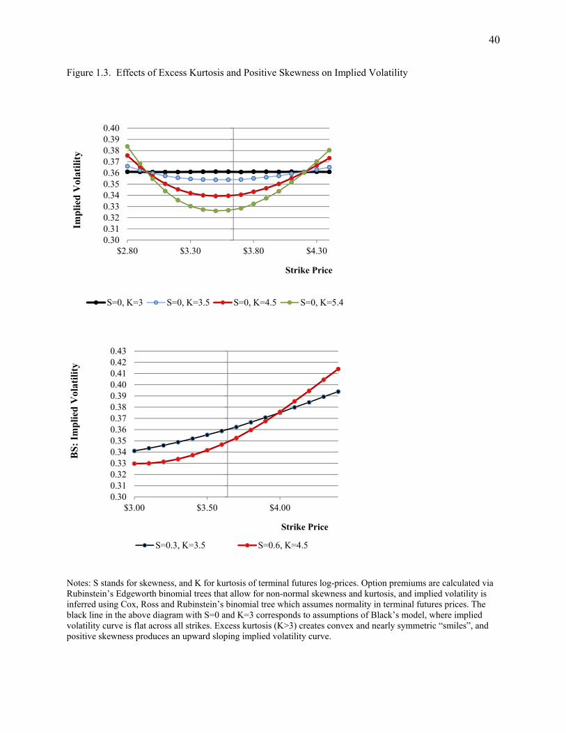
40
Figure 1.3. Effects of Excess Kurtosis and Positive Skewness on Implied Volatility
Notes: S stands for skewness, and K for kurtosis of terminal futures log-prices. Option premiums are calculated via Rubinstein’s Edgeworth binomial trees that allow for non-normal skewness and kurtosis, and implied volatility is inferred using Cox, Ross and Rubinstein’s binomial tree which assumes normality in terminal futures prices. The black line in the above diagram with S=0 and K=3 corresponds to assumptions of Black’s model, where implied volatility curve is flat across all strikes. Excess kurtosis (K>3) creates convex and nearly symmetric “smiles”, and positive skewness produces an upward sloping implied volatility curve.
0.300.310.320.330.340.350.360.370.380.390.40
$2.80 $3.30 $3.80 $4.30
Imp
lied
Vol
atil
ity
Strike Price
S=0, K=3 S=0, K=3.5 S=0, K=4.5 S=0, K=5.4
0.300.310.320.330.340.350.360.370.380.390.400.410.420.43
$3.00 $3.50 $4.00
BS
: Im
pli
ed V
olat
ilit
y
Strike Price
S=0.3, K=3.5 S=0.6, K=4.5

41
Figure 1.4. New Crop Price Distributions Conditional on Storage Adequacy
Note: Reproduced from Williams and Wright (1991). Conditional price distributions obtained from a rational expectations competitive equilibrium model with storage. The time frequency is one year, i.e. t+1 represents the next harvest. New crop price distributions are conditional on information known after old crop carryout stocks have been determined, but before weather shocks are revealed. Prices and quantity are standardized to make non-stochastic equilibrium at $100 and 100 units. Higher prices at time t reflect lower carryout stocks, and correspond to higher skewness of new crop price distribution.
Figure 1.5. Weather Stress in the Corn Crop
Note: Reproduced from Shaw et al. (1988). This figure shows the relationship between the age of the corn crop and the percentage yield reduction due to one day of moisture stress. Outer lines show boundaries of experimental results, while the middle line shows the average.
Price in period t+1
Probability
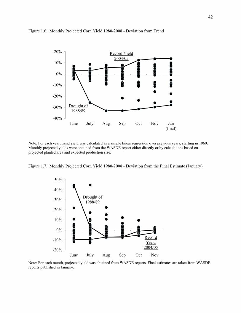
42
Drought of 1988/89
Record Yield 2004/05
-40%
-30%
-20%
-10%
0%
10%
20%
June July Aug Sep Oct Nov Jan(final)
Drought of 1988/89
Record Yield
2004/05-20%
-10%
0%
10%
20%
30%
40%
50%
June July Aug Sep Oct Nov
Figure 1.6. Monthly Projected Corn Yield 1980-2008 - Deviation from Trend
Note: For each year, trend yield was calculated as a simple linear regression over previous years, starting in 1960. Monthly projected yields were obtained from the WASDE report either directly or by calculations based on projected planted area and expected production size.
Figure 1.7. Monthly Projected Corn Yield 1980-2008 - Deviation from the Final Estimate (January)
Note: For each month, projected yield was obtained from WASDE reports. Final estimates are taken from WASDE reports published in January.
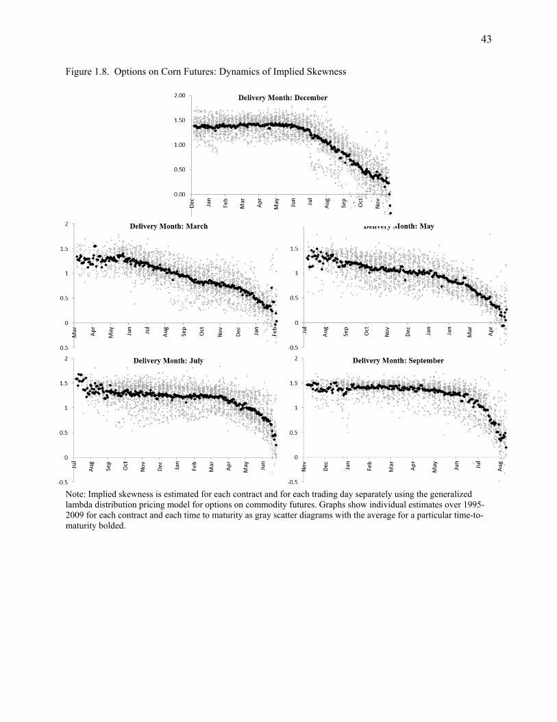
43
Figure 1.8. Options on Corn Futures: Dynamics of Implied Skewness
Note: Implied skewness is estimated for each contract and for each trading day separately using the generalized lambda distribution pricing model for options on commodity futures. Graphs show individual estimates over 1995-2009 for each contract and each time to maturity as gray scatter diagrams with the average for a particular time-to-maturity bolded.

44
Figure 1.9. Relationship between Implied Skewness and Expected Ending Stocks-to-Use
Note: Years with increase in intended cultivated acreage of 5 or more percent are drawn using green rhombs. Years with the June-to-June increases in the unemployment rate of 1 percent or more are drawn using blue triangles.
1995
1996
1997
1998
1999
2000
20012002
2003
2004
2005
2006
2007
20091.05
1.15
1.25
1.35
1.45
1.55
4% 6% 8% 10% 12% 14% 16% 18% 20% 22%
Imp
lied
Sk
ewn
ess
Ending Stocks-To-Use

45
Figure 1.10. Predicted Intra-Year Dynamics of Implied Skewness for Options on Corn Futures Contracts
Note: Implied skewness is modeled with quadratic segments with one regime switch. The grayed area covers the corn growth sensitive period, i.e. silking through harvest time (approximately Jun 20 – Oct 20).
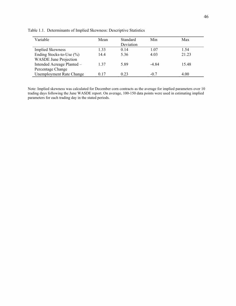
46
Table 1.1. Determinants of Implied Skewness: Descriptive Statistics
Variable Mean Standard Deviation
Min Max
Implied Skewness 1.33 0.14 1.07 1.54 Ending Stocks-to-Use (%) WASDE June Projection
14.4 5.36 4.03 21.23
Intended Acreage Planted – Percentage Change
1.37 5.89 -4.84 15.48
Unemployment Rate Change 0.17 0.23 -0.7 4.00
Note: Implied skewness was calculated for December corn contracts as the average for implied parameters over 10 trading days following the June WASDE report. On average, 100-150 data points were used in estimating implied parameters for each trading day in the stated periods.
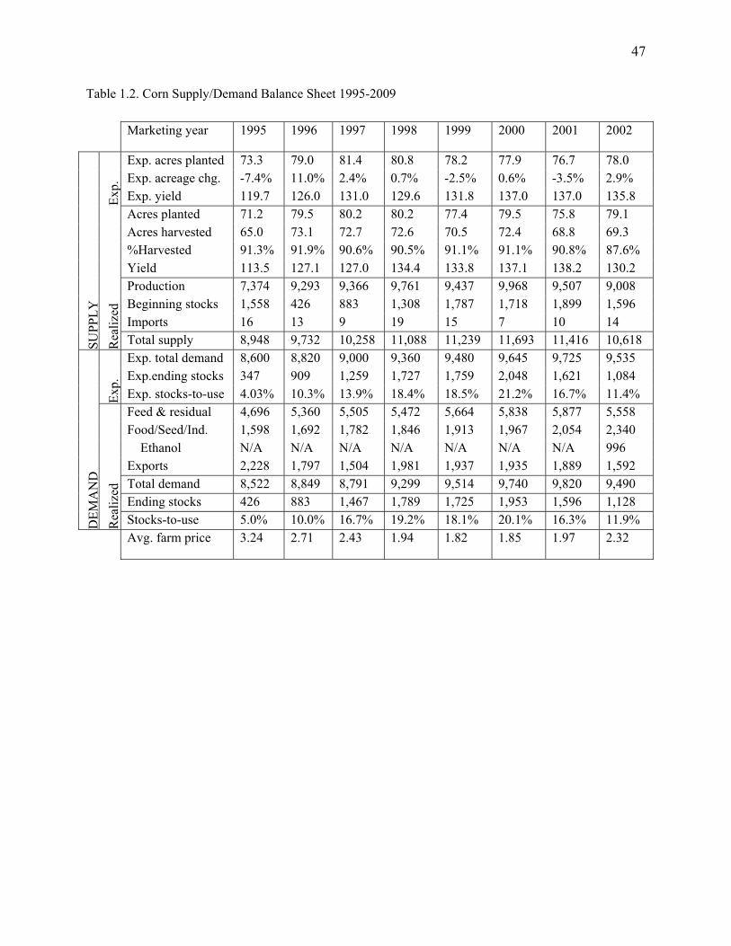
47
Table 1.2. Corn Supply/Demand Balance Sheet 1995-2009
Marketing year 1995 1996 1997 1998 1999 2000 2001 2002
SU
PP
LY
Exp
.
Exp. acres planted 73.3 79.0 81.4 80.8 78.2 77.9 76.7 78.0 Exp. acreage chg. -7.4% 11.0% 2.4% 0.7% -2.5% 0.6% -3.5% 2.9% Exp. yield 119.7 126.0 131.0 129.6 131.8 137.0 137.0 135.8
Rea
lize
d
Acres planted 71.2 79.5 80.2 80.2 77.4 79.5 75.8 79.1 Acres harvested 65.0 73.1 72.7 72.6 70.5 72.4 68.8 69.3 %Harvested 91.3% 91.9% 90.6% 90.5% 91.1% 91.1% 90.8% 87.6% Yield 113.5 127.1 127.0 134.4 133.8 137.1 138.2 130.2 Production 7,374 9,293 9,366 9,761 9,437 9,968 9,507 9,008 Beginning stocks 1,558 426 883 1,308 1,787 1,718 1,899 1,596 Imports 16 13 9 19 15 7 10 14 Total supply 8,948 9,732 10,258 11,088 11,239 11,693 11,416 10,618
DE
MA
ND
Exp
.
Exp. total demand 8,600 8,820 9,000 9,360 9,480 9,645 9,725 9,535 Exp.ending stocks 347 909 1,259 1,727 1,759 2,048 1,621 1,084 Exp. stocks-to-use 4.03% 10.3% 13.9% 18.4% 18.5% 21.2% 16.7% 11.4%
Rea
lize
d
Feed & residual 4,696 5,360 5,505 5,472 5,664 5,838 5,877 5,558 Food/Seed/Ind. 1,598 1,692 1,782 1,846 1,913 1,967 2,054 2,340 Ethanol N/A N/A N/A N/A N/A N/A N/A 996 Exports 2,228 1,797 1,504 1,981 1,937 1,935 1,889 1,592 Total demand 8,522 8,849 8,791 9,299 9,514 9,740 9,820 9,490 Ending stocks 426 883 1,467 1,789 1,725 1,953 1,596 1,128 Stocks-to-use 5.0% 10.0% 16.7% 19.2% 18.1% 20.1% 16.3% 11.9%
Avg. farm price 3.24 2.71 2.43 1.94 1.82 1.85 1.97 2.32
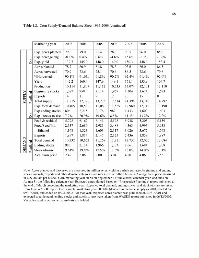
48
Table 1.2. Corn Supply/Demand Balance Sheet 1995-2009 (continued)
Note: Acres planted and harvested are measured in million acres, yield in bushels per acre, beginning and ending stocks, imports, exports and other demand categories are measured in million bushels. Average farm price measured in U.S. dollars per bushel. Corn marketing year starts on September 1 of the current calendar year, and ends on August 31 the following calendar year. Expected acres planted based on “Prospective Plantings” report published at the end of March preceding the marketing year. Expected total demand, ending stocks, and stocks-to-use are taken from June WASDE report. For example, marketing year 2001/02 (denoted in the table simply as 2001) started on 09/01/2001, and ended on 08/31/2002. For that year, expected acres planted was published on 03/31/2001 and expected total demand, ending stocks and stocks-to-use were taken from WASDE report published in 06/12/2002. Variables used in econometric analysis are bolded.
Marketing year 2003 2004 2005 2006 2007 2008 2009
SU
PP
LY
Exp
.
Exp. acres planted 79.0 79.0 81.4 78.0 90.5 86.0 85.0 Exp. acreage chg. -0.1% 0.4% 0.6% -4.6% 15.6% -8.1% -1.2% Exp. yield 139.7 145.0 148.0 149.0 150.3 148.9 153.4
Rea
lize
d
Acres planted 78.7 80.9 81.8 78.3 93.6 86.0 86.5 Acres harvested 70.9 73.6 75.1 70.6 86.5 78.6 79.6 %Harvested 90.1% 91.0% 91.8% 90.2% 92.4% 91.4% 92.0% Yield 142.2 160.4 147.9 149.1 151.1 153.9 164.7 Production 10,114 11,807 11,112 10,535 13,074 12,101 13,110 Beginning stocks 1,087 958 2,114 1,967 1,304 1,624 1,673 Imports 14 11 9 12 20 15 8 Total supply 11,215 12,776 13,235 12,514 14,398 13,740 14,792
DE
MA
ND
Exp
.
Exp. total demand 10,405 10,560 11,060 11,525 12,960 12,140 13,190 Exp.ending stocks 806 2,215 2,176 987 1,433 1,600 1,603 Exp. stocks-to-use 7.7% 20.9% 19.6% 8.5% 11.1% 13.2% 12.2%
Rea
lize
d
Feed & residual 5,798 6,162 6,141 5,598 5,938 5,205 5,159 Food/Seed/Ind. 2,537 2,686 2,981 3,488 4,363 4,993 5.938 Ethanol 1,168 1,323 1,603 2,117 3,026 3,677 4,568 Exports 1,897 1,814 2,147 2,125 2,436 1,858 1,987 Total demand 10,232 10,662 11,269 11,211 12,737 12,056 13,084 Ending stocks 983 2,114 1,966 1,303 1,661 1,684 1,708 Stocks-to-use 9.61% 19.8% 17.5% 11.6% 13.0% 14.0% 13.1%
Avg. farm price 2.42 2.06 2.00 3.04 4.20 4.06 3.55
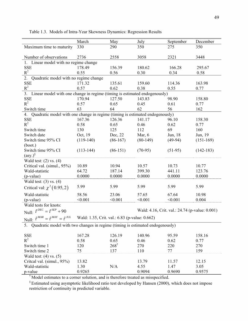
49
Table 1.3. Models of Intra-Year Skewness Dynamics: Regression Results
March May July September December Maximum time to maturity
330 290 350 275 350
Number of observations 2736 2558 3058 2321 3448 1. Linear model with no regime change SSE 178.49 156.39 180.62 166.28 295.67 R2 0.55 0.56 0.30 0.34 0.58 2. Quadratic model with no regime change SSE 171.32 135.61 159.60 114.36 163.98 R2 0.57 0.62 0.38 0.55 0.77 3. Linear model with one change in regime (timing is estimated endogenously) SSE 170.94 127.50 143.83 98.90 158.80 R2 0.57 0.65 0.45 0.61 0.77 Switch time 63 64 62 56 162 4. Quadratic model with one change in regime (timing is estimated endogenously) SSE 167.36 126.36 141.17 96.10 158.30 R2 0.58 0.65 0.46 0.62 0.77 Switch time 130 125 112 69 160 Switch date Oct, 19 Dec, 22 Mar, 6 Jun, 18 Jun, 19 Switch time 95% CI (boot.)
(119-140) (86-167) (80-149) (49-94) (151-169)
Switch time 95% CI (asy.)§
(113-144) (86-151) (70-95) (51-95) (142-183)
Wald test: (2) vs. (4) Critical val. (simul., 95%) 10.89 10.94 10.57 10.73 10.77 Wald-statistic 64.72 187.14 399.30 441.11 123.76 (p-value) 0.0000 0.0000 0.0000 0.0000 0.0000 Wald test: (3) vs. (4)
Critical val: 2 0.95, 2 5.99 5.99 5.99 5.99 5.99
Wald-statistic 58.56 23.06 57.65 67.64 10.98 (p-value) <0.001 <0.001 <0.001 <0.001 0.004 Wald tests for knots:
Null: 90DEC SEP Wald: 4.16, Crit. val.: 24.74 (p-value: 0.001)
Null: MAR MAY JUL Wald: 1.35, Crit. val.: 6.83 (p-value: 0.662)
5. Quadratic model with two changes in regime (timing is estimated endogenously) SSE 167.28 126.19 140.96 95.59 158.16 R2 0.58 0.65 0.46 0.62 0.77 Switch time 1 120 268† 270 220 270 Switch time 2 75 137 110 77 159 Wald test: (4) vs. (5) Critcal val. (simul., 95%) 13.82 13.79 11.57 12.15 Wald-statistic 1.30 N/A 4.55 1.47 3.05 p-value 0.9265 0.9094 0.9690 0.9575
† Model estimates to a corner solution, and is therefore treated as misspecified. § Estimated using asymptotic likelihood ratio test developed by Hansen (2000), which does not impose restriction of continuity in predicted variable.
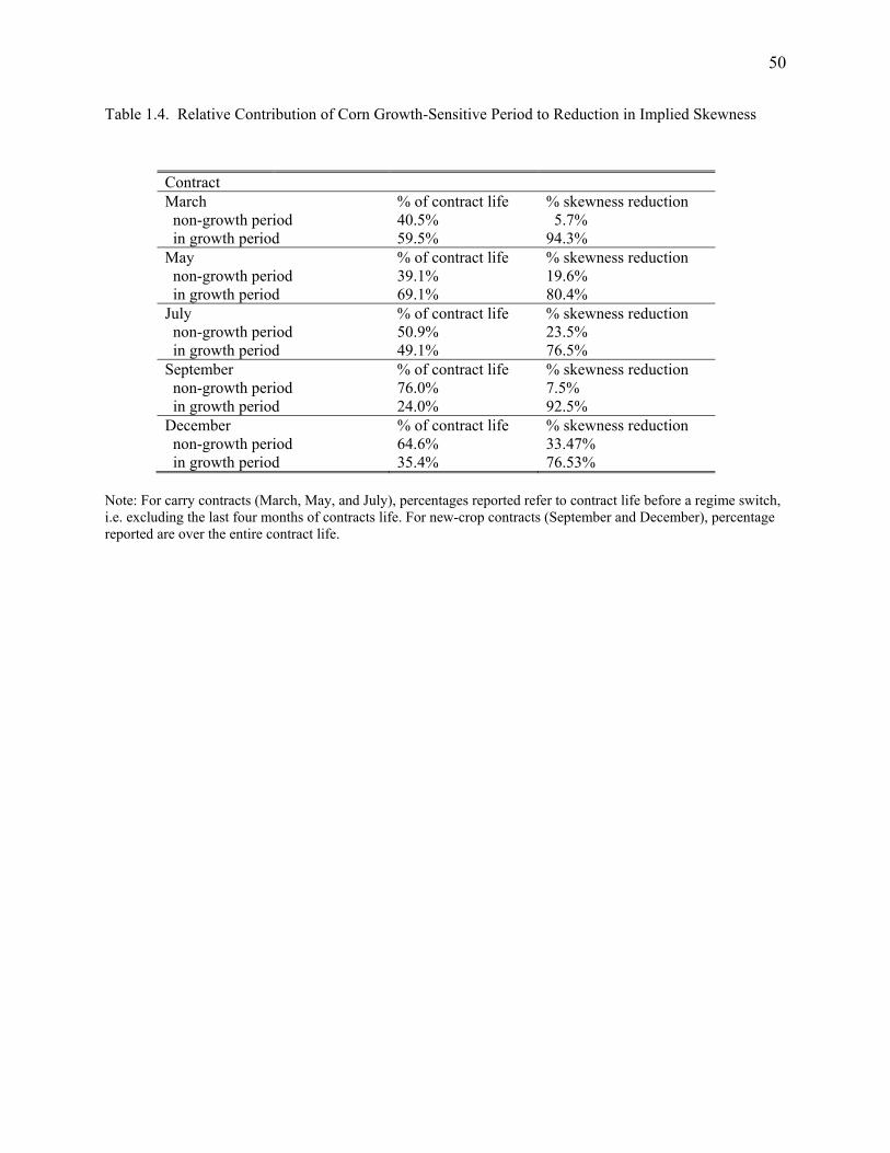
50
Table 1.4. Relative Contribution of Corn Growth-Sensitive Period to Reduction in Implied Skewness
Contract March % of contract life % skewness reduction non-growth period 40.5% 5.7% in growth period 59.5% 94.3% May % of contract life % skewness reduction non-growth period 39.1% 19.6% in growth period 69.1% 80.4% July % of contract life % skewness reduction non-growth period 50.9% 23.5% in growth period 49.1% 76.5% September % of contract life % skewness reduction non-growth period 76.0% 7.5% in growth period 24.0% 92.5% December % of contract life % skewness reduction non-growth period 64.6% 33.47% in growth period 35.4% 76.53%
Note: For carry contracts (March, May, and July), percentages reported refer to contract life before a regime switch, i.e. excluding the last four months of contracts life. For new-crop contracts (September and December), percentage reported are over the entire contract life.
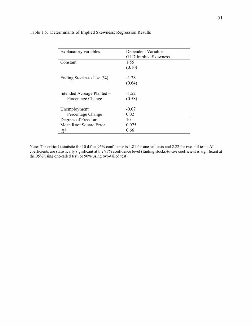
51
Table 1.5. Determinants of Implied Skewness: Regression Results
Explanatory variables Dependent Variable: GLD Implied Skewness
Constant 1.55 (0.10)
Ending Stocks-to-Use (%)
-1.28 (0.64)
Intended Acreage Planted – Percentage Change
-1.52 (0.58)
Unemployment Percentage Change
-0.07 0.02
Degrees of Freedom 10 Mean Root Square Error 0.075
2R 0.66
Note: The critical t-statistic for 10 d.f. at 95% confidence is 1.81 for one-tail tests and 2.22 for two-tail tests. All coefficients are statistically significant at the 95% confidence level (Ending stocks-to-use coefficient is significant at the 95% using one-tailed test, or 90% using two-tailed test).
52
2. Volatility Dynamics in Non-storable Commodities: A Case of Class III Milk Futures
ABSTRACT. This paper begins with an account of the evolution of dairy futures markets in the U.S. A
partially overlapping time series (POTS) model is then estimated to examine price behavior in
simultaneously traded Class III milk futures contracts. POTS is a latent factor model that measures price
changes in futures as a linear combination of a common factor, i.e. information affecting all traded
contracts, and an idiosyncratic term specific to each contract. This paper contributes to the literature by
showing that the importance of a common factor in price volatility determination for dairy is related to
capital production factors, i.e. the dairy herd. Finally, it is shown that Class III milk futures volatility
decreases as contracts approach maturity. This “Inverse Samuelson Effect” comes from the fact that Class
III milk futures are cash-settled contracts that settle against a formula-based price. The results suggest that
the importance of the common factor declines as one approaches maturity, implying that individual
contract months are poor substitutes in hedging a specific month’s cash price risk. Thus, despite low
liquidity in the market, it is useful to have 12 contract delivery months per year.
JEL Codes: G13, Q14
Keywords: Partially overlapping time series model, EM algorithm, dairy futures, volatility
53
2.1. Introduction
The U.S. Dairy industry has undergone significant change over the last two decades. Some of the
more salient features include continued increases in yield, regional shifts in production
accompanied by an increasing role of large farms, and major changes in dairy policy and milk
pricing (Blayney (2002), Blayney et al. (2006), Bozic and Gould (2009)). Over the last two
decades federal price supports have been low relative to market prices, and the volatility of milk
price volatility has increased dramatically across all categories of milk utilization. This
increasingly uncertain economic environment resulted in the development of new instruments for
managing price risk in the early 1990’s. Beginning in 1993, futures contracts were introduced to
meet the hedging needs of the dairy sector. However, in response to regular changes in both
industry practices and public policy, dairy futures contracts have gone through continuous re-
design.
Several papers have been written on the performance of specific dairy futures contracts
(Fortenbery, Cropp, and Zapata (1997), Fortenbery and Zapata (1997), and Maynard, Wolf, and
Gearhardt (2005)) but a detailed exposition of their history and performance is still lacking. This
represents the first contribution of this paper.
To evaluate the performance of a futures contract, it is essential to understand the price volatility
dynamics including seasonality, time-to-maturity effects, and cash-futures volatility spillovers, as
well as the effects of speculation and liquidity. This paper addresses the first two topics using
the Class III milk futures contract. This contract exhibits the highest trade volume among the
family of dairy futures contracts. Cash-futures volatility and speculative impacts on dairy prices
are the subject of a parallel study.
54
There are two characteristics that differentiate the Class III milk contract from many other
agricultural futures contracts. First, milk is essentially a non-storable product, and the only way
to partially preserve or enhance the economic value of milk over time is to undertake an
irreversible conversion to one of the derived dairy products. Another differentiating
characteristic is that Class III milk contracts are not settled by physical delivery. They are cash
settled against the USDA announced Class III milk price based on a publicly known formula.
This raises two research questions. First, for storable commodities, temporal arbitrage
opportunities guarantee that information affecting a futures price for a certain maturity will also
have an impact on all other traded delivery periods. Does the perishable nature of milk result in
information pertinent to one contract having little or no influence on the price of any other
contract? Second, in storable commodities, volatility normally increases as time to maturity
declines (Smith (2005)). This is called the ‘Samuelson Effect,’ after Paul Samuelson (1965) who
first proposed the conditions under which such a relationship exists. But if milk futures are cash
settled against a formula-based price, and the USDA formula is both transparent and based to a
large extent on information known prior to contract expiration, should we still expect to see a
Samuelson Effect? Addressing these issues is the second and most important contribution of this
paper.
The paper proceeds as follows: in the next section we provide an outline of the economic
environment faced by the US milk industry. This is followed by a description of the history of
dairy futures contracts including a review of previous work analyzing dairy futures. Section 2.4
introduces the POTS model and the data used to analyze dairy futures price performance. In
section 2.6 we present the main econometric results. The final section discusses consequences of
the results, and draws conclusions related to the structure of the Class III milk futures market.

55
2.2. Overview of Dairy Futures Contracts
2.2.1. Evolution of Dairy Futures
U.S. milk prices were relatively stable through the late 1980’s as government price supports were
generally binding. In the early1990’s, however, milk price volatility increased significantly as
both support prices and government stocks of dairy products were reduced. This has been
widely reported and can be seen in Figure 2.1.
In response to increased price volatility tools were developed to help the dairy sector
manage its new market price risk. The first dairy futures contracts were introduced by the
Coffee, Sugar, and Cocoa Exchange (CSCE - now part of the New York Board of Trade) in New
York in 1993. The initial impetus for the development of dairy futures came from the cheese and
confectionary industries. Cheese makers were concerned about price volatility in cheddar cheese
and milk, as cheddar is used as the reference price for many cheeses produced domestically. At
the same time the confectionary industry was concerned with increased price volatility in non-fat
dry milk, an important ingredient in candy making (Fortenbery (2009)). Many of the
confectionary firms were hedging cocoa and sugar at the CSCE, and once they began to
experience price volatility in non-fat dry milk they wanted a way to manage that risk as well.
Since the confectionary firms were already using contracts traded at the CSCE, this seemed the
logical place to launch the non-fat dry milk contract. As a result, the CSCE rolled out a cheddar
cheese and a non-fat dry milk futures contract in 1993. Since prices for cheddar cheese and milk
are highly correlated, it was assumed that other dairy firms, including dairy farmers, would cross
hedge their milk price risk with the cheddar cheese futures contract. However, despite a
significant promotional effort on the part of the exchange, initial trade volume was very thin.

56
One reason for thin volume was the lack of cross hedging of milk in cheese futures. In response,
the CSCE developed and launched a futures contract for fluid milk in 1995, but this contract also
suffered low trade volume. Despite the low participation in dairy contracts at the CSCE,
however, the Chicago Mercantile Exchange (CME) launched a nearly identical fluid milk
contract in 1996. This marked the first time since wheat in the 1950’s that two domestic futures
exchanges competed head to head for trade in nearly identical products. The competition
intensified when both exchanges launched a butter futures contract in 1996. Like the earlier
dairy contracts, however, trade in butter futures was also nearly non-existent.
The next change in dairy contract design was in response to changes in federal milk policy. In
1997, both exchanges re-designed their fluid milk contracts, and converted them to a Basic
Formula Price contract (BFP). The BFP was introduced in 1995 and was the USDA’s monthly
announced price from which prices paid to individual dairy farmers were derived. The BFP was
based on USDA survey data adjusted by a product price formula. Since the BFP contracts were
explicitly cash settled against the USDA BFP announced price that determined individual
farmers’ prices they provided a direct hedge opportunity for dairy producers.
In addition to its BFP contract, the CME launched a cheddar cheese contract in 1997. Once this
happened the only unique contract still in existence in New York was the non-fat dry milk
contract. However, this did not last long. In 1998, the Chicago Exchange rolled out both a dry
milk and a dry whey futures contract. In 2000, the New York market eliminated its dairy
contracts, and Chicago became the sole market for the trade of dairy futures.
Following requirements set forth in the 1996 Farm Bill, new milk pricing classes were
introduced in January 2000. These replaced the BFP formula price. The Class III milk price was
developed to reflect the minimum price for milk used to make cheese, while Class IV was
57
introduced for milk used in products such as butter and non-fat dry milk. The fundamental
change was that the BFP price had been based on surveyed purchase prices of manufacturing
grade milk, while the new formulas were based on wholesale prices of products that used
manufacturing milk as an input. Consequently, the BFP and cheddar cheese futures contracts
were replaced with a Class III milk contract. In addition, the nonfat dry milk and dry whey
contracts were discontinued, and a new Class IV milk contract was introduced.
Responding to requests from industry, CME continued to make changes to their dairy futures
products over the next several years. A cash-settled butter contract was introduced in 2005 with
a contract size equal to half the old physically delivered butter contract. Cash settled dry whey
was introduced in March 2007. A nonfat dry milk cash-settled contract, discontinued in 2000,
was redesigned and introduced in 2008. This was followed by a physically delivered nonfat dry
milk contract in 2009, and deliverable cheese and international skim milk powder in 2010. Table
2.1 summarizes the development and abandonment of the various dairy contracts from 1993
through 2010.
2.2.2. Price Relationships among Current Contracts
Correlations between selected dairy prices over the last 10 years are given in Table 2.2. Note that
the Class III price is strongly correlated with both cheddar cheese prices (National Agricultural
Statistics Service (NASS) survey prices for the last week of the month) and fluid milk prices.
The Class IV announced price is strongly correlated with fluid milk and nonfat dry milk prices.
Butter and dry whey show weak correlation with Class III and Class IV prices. This suggests a
need for separate futures contracts for these products if futures are to be used as risk management
vehicles. However, neither nonfat dry milk nor butter futures contracts reveal much trade

58
volume. Also, as of February 2011 open interest in the recently introduced deliverable cheese
contract was extremely low, and may be due to the high correlation with Class III futures.
2.3. Literature Review
Early papers (Fortenbery and Zapata (1997), Thraen (1999)) examined pricing issues in dairy
markets by measuring cointegration relationships between cheddar cheese cash and futures
prices. Fortenbery and Zapata (1997) failed to find a significant cointegrating vector between
prices, but argued that the market might not have been mature enough to establish a stable long-
run equilibrium at the time of their analysis. Using a longer time series, Thraen does find a
stable relationship between cash and futures prices for cheddar cheese.
Later, Fortenbery, Cropp and Zapata (1997), Zylstra, Kilmer and Uryasev (2004), and Maynard,
Wolf, and Gearhardt (2005) examined the hedging opportunities for fluid milk with milk futures
contracts. Fortenbery et al. evaluated the performance of the BFP milk contract, while the later
papers focused on the Class III contract. It was found that the BFP contract was successful in
reducing price risk for milk producers in the Upper Midwest, but less useful for producers on the
West Coast. Zylstra et al. examined basis risk for Class I milk producers hedging with the Class
III contract, and determined that basis risk prevented producers from locking in a minimum
Class I milk price using only the Class III futures. Hedging performance could be improved by
using a lagged futures position, and offsetting the hedge the day the Class I price is announced.
Maynard et al. found that hedging generally resulted in a 50 to 60 percent reduction in price
variance, but the markets favored large, sophisticated producers in major cheese manufacturing
regions.
Market efficiency issues were studied by Tondel and Maynard (2004) and Sanders and Manfredo
(2005). Tondel and Maynard focused on the butter market, and failed to reject the null

59
hypothesis of market efficiency in the deliverable butter contract. Sanders and Manfredo studied
the milk contract, and argued that milk futures do not encompass all the information contained in
USDA forecasts at a two-quarter horizon. However, they also found that the revenue obtained
by exploiting the difference in forecast performance is likely below transaction costs.
Buschena and McNew (2008) investigated the market impacts of the 1999 USDA Dairy Options
Pilot Program. The program sought to teach dairy producers how to use put options to hedge
downside price risk, and subsidized the purchase of the options. They found that options
purchased under the Pilot Program generally resulted in higher options premiums compared to
options not purchased through the program.
The low liquidity of dairy futures was a common theme in earlier work. This suggests there
might be a trade-off between liquidity and the number of different futures products offered, with
the introduction of new products leading to reductions of trading volume in existing products. In
addition, most successful agricultural futures contract do not trade for delivery every month.
Would decreasing the number of traded contract months be beneficial for milk futures in the
sense of higher liquidity and lower hedging costs? Our analysis of volatility dynamics in Class
III futures provides a conceptual framework for answering that question.
There has not been an extensive analysis of potential cyclical behavior in milk pricing, nor an
examination of possible structural breaks in milk price dynamics induced by changes in federal
dairy policy. It seems that U.S. dairy policy changes may have opened the door for a classic
boom-bust cycle in milk production, where initial periods of very low milk prices result in a

60
contraction of milk production that then leads to much higher prices. Higher prices then induce
new entrants or expansions of existing farms.5 This is the focus of Appendix 1.
2.4. Econometric Analysis
2.4.1. The POTS Model - Introduction
A common approach to studying volatility in futures markets is to construct a so called “nearby”
series, where only data from contracts closest to expiry are used. In such an approach, when the
nearby contract expires, or time-to-maturity falls below a certain predetermined number of
trading days, data used for the “nearby” series are drawn from the next-to-nearby contract. This
strategy creates a single time series which can then be used in econometric estimation. However,
this approach is not without its problems. By deciding to use information from only a single
contract on any given trading day, information from all other contracts is discarded.
Furthermore, the “rollover” procedure for patching consecutive contracts may introduce complex
non-linear dynamics .
In this paper we employ a partially overlapping time series (POTS) model similar to
Smith (2005) and Suenaga, Smith and Williams (2008). The POTS model utilizes information
from all contracts trading concurrently. The difference between a “nearby” and POTS approach
is illustrated in Figure 1.2 for Class III milk futures. In the POTS approach, each line represents a
new variable, while in the “nearby” approach only the bold segments of each contract trading
period are used and patched together consecutively to create a continuous time series. In this
context, the POTS model can be interpreted as an unbalanced panel method, as each contract
5 In Appendix 1 we a present spectral analysis of milk prices and find that the primary difference in sample spectrums for the periods 1970-1991 vs. 1988-2009 is the emergence of 3 year cycle in the later period.

61
constitutes a separate time series that originates on the first day the contract is traded, and
terminates at its’ last trading day.
POTS is a latent factor model where price changes on contracts are assumed to be linear
combinations of a common factor, i.e. information affecting all traded contracts, and an
idiosyncratic term specific to each contract. This ability to differentiate the impact and relative
importance of common factor and idiosyncratic effect is lost when considering only a nearby
price series. Smith finds that for corn and natural gas, the information sets pertinent to contracts
with different maturities show almost perfect overlap, i.e. the common factor explains close to
100 percent of futures price variance. However, it is the storable nature of these two
commodities that renders this an expected result.
In explaining the POTS model, we closely follow the terminology and notation of Smith (2005).
Let F denote the price of a futures contract, d the number of trading days until maturity for a
particular contract, and t the date of the observation. Then subscripting ,d tF suffices to uniquely
identify any point in a partially overlapping panel data set. Smith models sources of volatility in
futures prices as originating from a latent common factor t , influencing all currently trading
contracts, and idiosyncratic errors ,d tu , specific to each contract.
Modeling jointly all concurrently traded contracts, we can write:
t t t t t ΔF θ λ u (2.1)
where tΔF is the 1tn vector of price changes for contracts traded at time t . The common factor
is modeled as the scalar t with 20, 1t tE E and tθ is a 1tn vector of factor loadings
for each of the tn contracts that traded on date t . The vector tu represents idiosyncratic shocks
62
specific to each contract. For identification purposes, we assume that ~ 0,tt nN Iu ,
0, ,tE t u and 0tE u u for t . Finally, tλ is the diagonal t tn n matrix of the
innovations’ standard deviations. We assume futures prices are unbiased, i.e. 1| 0ttE ΔF
where 1t denotes the information set at 1t .
The factor loadings and innovation standard deviations are modeled using cubic splines with two
knots. As Smith explains, spline functions capture deterministic seasonal and time-to-delivery
effects. Separate splines are estimated for each delivery month. For a specific delivery month,
factor loadings and innovation standard deviation splines have the following functional form:
3 2 3
, 0 1 1 2 1 3 11
3 2 3
, 0 1 1 2 1 3 11
11
d t j j t j j t j j t j jtj
d t j j t j j t j j t j jtj
jt j t j
d k d k d k I
d k d k d k I
I k d k
(2.2)
where jtI is an indicator function, ij and ij are parameters estimated by the model, td is the
number of trading days to maturity on date t for a particular contract, and knots connecting
consecutive cubic functions, 1 2,k k are chosen a priori to be 30 and125 trading days to maturity.
Additional nodes are 0 0k at contract expiry and maxK tk d , i.e. maximal time-to-horizon
trade observed for this specific contract month. We impose several constraints on the splines.
First, consecutive cubic functions they must equal in value at the nodes. Letting t jd k , at knot
jk we have
63
2 3
0 1 0 1 1 2 1 3 1
2 3
0 1 0 1 1 2 1 3 1
j j j j j j j j j j j
j j j j j j j j j j j
k k k k k k
k k k k k k
(2.3)
Next, to stipulate smoothness, slopes of the adjoining cubic functions must be equal at knots.
Differentiating cubic functions with respect to td and setting the first derivatives equal to each
other, we obtain
2
1 1 1 2 1 3 1
2
1 1 1 2 1 3 1
2 3
2 3
j j j j j j j j
j j j j j j j j
k k k k
k k k k
(2.4)
Finally, we force the slope of both splines to equal zero at end points, i.e. at contract expiry and
at maximum time-to-maturity horizon observed in the data. Denoting maximal time-to-maturity
with Kk (maximum time-to-maturity is the last node), we get
2
11 1 2 1 3 1
2
11 1 2 1 3 1
0, 2 3 0
0, 2 3 0
K K K K K K K
K K K K K K K
k k k k
k k k k
(2.5)
Each spline is thus fully determined by 12 parameters, but given the restrictions imposed only 6
free parameters need to be estimated per spline. Class III milk futures trade for 12 contract
months per year, which brings the number of spline parameters that we need to estimate to 144;
72 coefficients for common factor splines, and as much for contract-specific innovation splines.
The time-varying conditional volatility in the common factor is modeled using a GARCH(1,1)
process. Denoting the conditional variance of the common factor as 2 2 1| tt th E , we have
2 2 2 11 1 | t
t t th h E (2.6)
To restrict the unconditional variance to be equal to 1, free parameter is constrained to be
1 .
64
Given the assumptions that idiosyncratic shocks are uncorrelated across contracts and over time,
the conditional covariance matrix, just like in Smith (2005), is given by
1 2 2| tt t t t t t tE h ΔFΔF θ θ λ (2.7)
2.4.2. Using Kalman Filter to Obtain Conditional Variance of the Common Factor
The only data directly observable are futures price changes, index classifying each observation to
one of 12 contract months and time to maturity. In particular, we do not observe the common
factor, and we need to use Kalman filter to obtain linear least squares forecast of the common
factor at time t, given the information set t . To do so, let us first summarize fundamentals of
state-space representation of dynamic systems. We follow closely exposition found in Hamilton
(1994, ch. 13). We first write down the most general state-space system using Hamilton’s
notation, and Kalman filter results pertinent to our analysis. We then map our model to state-
space representation and after considerable cancelations develop simple expressions for
conditional expectation | |t t t tE , and conditional variance of common factor
| | | |t t t t t t t t tP E .
Let us start by writing down the general state-space system equations. Following Hamilton, let
ty denote an 1n vector observed at time t . Possibly unobserved 1r vector tξ is called the
state vector. The state-space representation of the dynamics of ty is given by the state equation
1 1t t t ξ Gξ v (2.8)
where G is the matrix of parameters of dimensions r r and observation equation
t t t t y A x J ξ w (2.9)
65
where tx is a 1k vector of predetermined variables and A and J are matrices of parameters
of dimensions n k and n r .
The disturbances tv and tw are distributed normally with zero mean and covariances
for
0 otherwiset
t
tE v v
Q (2.10)
' for
0 otherwiset
t
tE
Rw w (2.11)
Finally, disturbances are uncorrelated at all lags:
0, ,tE v t w (2.12)
Hamilton motivates Kalman filter as an algorithm for calculating linear least squares forecasts of
the state vector on the basis of data we have observed through date t .
1| 1ˆ ˆ |t t t tE ξ ξ (2.13)
Kalman filter calculates these forecasts using a recursion, starting with 1|0ξ̂ then using that
forecast in obtaining 2|1ξ̂ and so on. Recursion is started with a forecast of 1ξ̂ based on no
previously observed data, i.e. using unconditional mean of 1ξ
1|0 1ˆ Eξ ξ (2.14)
with mean square error (MSE) of the forecast
1|0 1 1 't tP E E E ξ ξ ξ ξ (2.15)
Next, formula for forecasting ty is obtained
| 1 | 1ˆ t t t t t y A x J ξ (2.16)
66
Inference about the current value of tξ is updated on the basis of the observation of ty using
formula for updating a linear projection
| | 1 | 1 | 1
1
| 1 | 1 | 1
ˆ ˆ ˆ ˆ '
ˆ ˆ ˆ'
t t t t t t t t t t t
t t t t t t t t t t
E
E
ξ ξ ξ ξ y y
y y y y y y (2.17)
Finally, MSE of the updated projection, | | ' |t t t t t t tE ξ ξ ξ ξ , denoted |t tP is
1
| | 1 | 1 | 1 | 1't t t t t t t t t t
P P P J J P J R J P (2.18)
where | 1t tP is MSE of one-step ahead forecast of the state vector
| 1 1 1 1 't t t t t t t t tE E E P ξ ξ ξ ξ (2.19)
Rewriting the POTS model in state-space format, we see that there are no pre-determined
variables tx , i.e. 0 A , state equation is simplified by having 0G . Common factor t is
1 1 state vector, with state equation being
1 10t t tv (2.20)
Vector of observed variables is tF and coefficient next to state vector is time dependent, t tJ θ
so observation equation is
t t t t F θ w (2.21)
Common factor is uncorrelated through time, thus
| 1ˆ 0t t (2.22)
Together with equation (2.16) this implies that
| 1ˆ 0t tF (2.23)
To simplify expression (2.17) for updating the inference on the common factor at time t based on
data observed at time t, notice that
67
2 21 1 1t t t t t t t t t t t t tE E E h F θ w θ θ (2.24)
Based on (2.22), (2.23), (2.24) and (2.7), we find that updated inference on the common factor
can be written as
2 1|t t t t t th θ F (2.25)
Notice that equation (2.18) can be rewritten using the fact that 2| 1t t h P , 2
t tR λ and
2| 1' t t t t t th J P J R θ θ λ :
2 4 1|t t t t t t tP h h θ θ (2.26)
In equation (2.6) expression 21 1|t tE can now be expressed with the help of (2.25) and (2.26)
:
21 1 1| 1 1| 1 1| 1|t t t t t t t tE P (2.27)
Now we have everything in place to recursively calculate conditional variances of the common
factor. Unconditional variance of the common factor is one, so recursion is started by setting
21 1h . To calculate 2
2h we need to calculate 2 21 1 1|1 1|1|E P . From (2.25) we calculate
2 11|1 1 1 1 1h θ F and 2 4 1
1|1 1 1 1't tP h h θ θ . After obtaining 22h we repeat the same procedure to
calculate 23h , and so on. Of course, everything that is written in this section assumes that
parameters of the model are known, while in fact they need to be estimated. We explain the
estimation procedure in detail in the next section.
2.4.3. Estimating POTS Model
Conditional on information available at 1t , futures price change is assumed to be normally
distributed with zero mean and conditional variance t developed in (2.7). Unbiasedness of
futures prices is evident from Figure 2.4, thus zero mean assumption does not seem to be
68
violated. Assumption of normality is not as binding due to classical results on consistency and
asymptotic normality of coefficient estimates obtained using quasi-maximum likelihood.
Therefore, to estimate the model, we need to maximize the Gaussian log-likelihood function:
11
1
1 1
log |
1 1log 2 log
2 2 2
T
t tt
T T
t t t tt t
L f
nT
F
F F
(2.28)
where 11
Tt tn T n is the average number of contracts traded each day, and tn is the number of
contracts traded on day t . Therefore, nT is simply the total number of observations. All
parameters that need to be estimated enter the likelihood function through the conditional
covariance matrix t . Combining (2.6) and (2.7) we can write
2 2 1 21 1 | t
t t t t t th E
θ θ λ (2.29)
Now we immediately see that unobserved common factor will make estimation of the likelihood
function complicated. To facilitate estimation we rewrite the likelihood function for a single
trading day as follows:
1 1 1| | , |t t t t t t tf f f ΔF ΔF (2.30)
Taking logs, we get
1 1 1log | log | , log |t t t t t t tf f f F F (2.31)
The first term in the sum in (2.31) is now much simplified due to conditioning on information
about the common factor. If we could observe the common factor t , we could be directly
maximizing the ‘complete data’ likelihood written below.
2
1 1
2 2 2
1 1
1log 2 log '
2 2
1 1log 2 log
2 2 2
T T
C t t t t t t t tt t
T T
t t tt t
nTL
Th h
λ F θ λ F θ
(2.32)
69
However, we do not observe t so the way forward is to iterate between using Kalman filter to
compute expected complete data likelihood, given parameters, and maximizing expected
likelihood with respect to the parameters. Using (2.27), we write the expected complete data
likelihood as follows:
2| |
1 1
2 2 2 2 2| | |
1 1 1
1| log 2 log '
2 2
1 1 1 1log 2 log
2 2 2 2 2
T T
C T t t t t t t t t t tt t
T T T
t t t t t t t t t t t tt t t
nTE L
TP h h h P
λ F θ λ F θ
θ λ θ
(2.33)
In maximizing (2.33) we use EM algorithm developed by Dempster et al. (1977), modified as in
Smith (2005). Computing the expectation of the complete data likelihood with respect to the
latent variable is called the E-step, and maximizing the expected likelihood with respect to the
parameters is referred to as the M-step. Algorithm is the following:
1) Make an initial guess about the parameters. For conditional variance of the common
factor, initial guess for coefficient in equation (2.6) is 0.08, and for coefficient it is
0.90. To obtain initial guess for spline parameters notice first that from
Error! Reference source not found. it follows that each spline is linear in x , where x
consists of products of indicator functions and exponents of time-to-next-knot counters.
For example, 2
0 1 0 0 1 2 0 0 11; ; , .t t t tx x d k I k d k x d k I k d k etc
Initial guesses for theta-splines (splines for common factor, separate spline for each
contract month) are obtained by projecting absolute values of dependent variable (futures
price changes) on x , then multiplying projection coefficients by 0.7. For lambda-splines
(contract-specific shocks) vectorized mean absolute value of dependent variable is
projected on x . Both projections are appropriately modified to account for restrictions
(2.3), (2.4) and (2.5).
70
2) Using current guess for spline and GARCH parameters, use the Kalman filter to obtain
|t t and |t tP .
3) Keeping both free GARCH parameters fixed, Newton-Raphsen is used in M-step to
maximize (2.33)
4) Steps 2 (E-step) and 3 (M-step) are iterated until convergence, not changing GARCH
parameters.
5) Now keeping spline parameters fixed, maximize likelihood with respect to GARCH
parameters.
6) Step 2-5 are repeated until convergence.
7) Parameter estimates obtained upon convergence in step 6 are used as starting values in
final numerical optimization over both spline and GARCH parameters using BHHH
algorithm.
2.5. Data
The POTS model for dairy futures is estimated using the Class III futures contracts because they
have the highest daily trading volume of all dairy futures, and an open interest that is generally
four times larger than the open interest of all other dairy futures combined. Class III futures are
cash settled against the announced USDA Class III milk price. Although this contract is used for
hedging manufacturing and fluid grade milk, both of which are non-storable commodities, the
settlement price is determined by the price of three dairy products, two of which are storable:
cheddar cheese (not storable), butter (storable) and dry whey (storable). 6
6 One could argue that cheddar cheese is storable, but through storage it is aged and that changes its value. The USDA price surveys used to calculate the Class III milk price exclude cheese sold that is over 30 days old.

71
Every week, NASS surveys all cheese, butter, dry whey and nonfat dry milk plants that
commercially produce more than 1 million pounds of these products, and computes national
average prices for each product. The Class III milk price is then calculated once a month using
a USDA formula that is based on the monthly weighted average prices of the products. The milk
pricing formula is rather complex. The three product prices are first used to calculate imputed
prices of milk components, i.e. protein, butterfat and other solids. In the second step, milk
component prices enter the formula to get a skim milk price. Finally, the Class III milk price is
calculated using the base skim milk price and assuming 3.5% butterfat content. Conflating this
multi-step USDA formula into a simple linear function of cheese, butter and dry whey prices
suggests that most of the manufacturing grade milk value comes from cheese. For example,
Class III milk price for October 2008 was announced the Agricultural Marketing Service on
October 31, 2008 at $17.06 per cwt. It was based on wholesale prices cheddar cheese, dry whey
and butter observed in weeks ending on 10/4, 10/11, 10/18, and 10/25. Weighted average
monthly prices for these commodities were calculated using weekly sales data. In the end, cheese
accounted for 86.08% of the milk price, while butter and dry whey contributed 2.55% and
11.37%, respectively. Full calculation is presented in Table 2.3.
Figure 2.3 presents the open interest (aggregated over all traded contract months) and the nearby
Class III futures price for the period 2000-2009. Three patterns emerge from this figure. First,
open interest shows an upward trend from 2000 through 2007, then flattens to an average level of
25,000 contracts. Second, open interest exhibits strong seasonality that corresponds to the
production patterns in milk, with a peak in May or June. Finally, the milk price and open interest
are strongly positively correlated. This is not un-expected - as milk prices increase, users of
72
manufacturing milk will likely hedge more of their input costs, and farmers may feel more
inclined to lock in a good price for their product.
The Class III price announcement refers to the Class III price for the previous month. For
example, the October 2010 Class III milk price was announced on Nov, 5 2010. This implies that
in contrast to other agricultural contracts, Class III futures trade through their delivery month.
Trade ends the business day immediately preceding the day on which USDA announces the
Class III price.
Data used for model estimation covers the period January 2000 through October 2009. Initially,
trading in Class III futures was allowed for up to 12 months prior to maturity. This was later
expanded to 18 months, and then to 24 months. However, there is very little volume for
contracts more than 1 year out so we restrict our analysis to the daily closing prices for the 12
most nearby contracts. This results in 28,145 data points over 118 contracts, classified in 12
categories based on the contract delivery month. Over the entire data period, average futures
price change is 0.125 cents with a standard deviation is 13.21 cents. The largest day-to-day drop
in price is $1.00 per cwt., and the largest increase is 95 cents. The distribution of price changes
is leptokurtic, with an excess kurtosis of 7.82. It is also slightly left-skewed with a skewness of -
0.14.
2.6. Results
To understand price dynamics in dairy markets, we first investigate whether futures prices appear
unbiased. As noted earlier, this is an explicit assumption in the POTS model. If prices are
unbiased, then we would expect the prediction errors associated with using futures price as an
expectation of later cash price to average zero. In other words, futures would not systematically
over or under predict cash prices. This is a necessary condition for futures price efficiency and
73
thus for the market to effectively provide for price discovery. To examine this we calculate, for
each futures contract at time t with d days to maturity, the percentage difference between the
current futures price ,d tF and the terminal settlement price TP . Note that TP is unknown before
expiration time T , and only discovered ex post. Realized percentage prediction errors, ,d tE are
thus calculated as
,,
,
100d t Td t
d t
F PE
F
(2)
Using scatter diagrams, plots of prediction errors are developed, with time to maturity d on the
x-axis and percentage prediction errors ,d tE on the y-axis. If the mean of ,d tE is below zero,
evidence exists that d days to maturity futures prices are systematically downward biased. This
result would be consistent with the Keynesian concept of a positive marginal risk premium. If,
on the other hand, mean of ,d tE is significantly above zero, that implies that futures prices exhibit
a systematic upward bias.
Figure 2.4 presents realized prediction errors for the period 2000-2009. Gray dots represent
individual prediction errors, while the bold black line plots root mean square prediction error for
each time-to-maturity d . Market efficiency postulates that prediction errors would be centered
around zero, so the appropriate measure of prediction accuracy is the root mean square error
(RMS). The RMS at 30 days to maturity is 2.77%, but rises to 14.20% 90 days and 27.76% one
year to maturity. We find that futures price prediction errors are centered around zero up to 180
days to maturity, but exhibit weak evidence of under prediction bias for time-to-maturity
horizons higher than 60 days, reaching a maximum 4.5% negative bias 350 days to maturity. We
do not explicitly examine the statistical properties of this bias, but given the high degree of
74
correlation of prediction errors at such distant horizons, and a root mean square error of 26.65%
at 350 days to maturity, we do not expect the bias to be statistically significant. We therefore do
not reject the assumption of un-biased futures prices. As a result, the POTS model was
estimated, and the empirical results are given in Appendix II. A description of the estimation
implications follows.
Given un-biasedness, the first issue to be addressed focuses on seasonal and time-to-
maturity effects on the volatility of futures prices. Second, the degree to which a common
information set is relevant to pricing futures with different maturities is examined. From
equation (2.1) it follows that the price change for an ith-nearby contract at time t is given by
, , , ,i t d t t d t i tF u where subscript i on both the price change and idiosyncratic shock
identifies a specific contract. The subscript id T t is the number of trading days left to
maturity for this contract. The factor loading ,d t and standard deviation of the idiosyncratic
shock ,d t are both deterministic functions of time to maturity and contract month. By imposing
unit variances on both the common factor and idiosyncratic shock, we can obtain the
unconditional variance of the price change for a specific contract as
2 2, , ,i t d t d tVar F
(3)
We can then easily calculate the fraction of variance due to information innovations pertinent to
all contracts, i.e. the common factor as
2,
, 2 2, ,
d ti t
d t d t
CFI F
(4)
where we denote this as the common factor importance to the i-th nearby contract at time t .
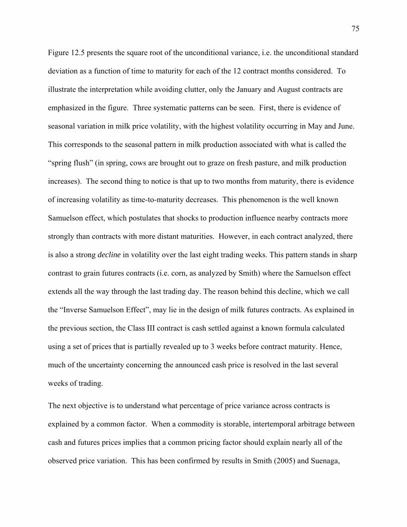
75
Figure 12.5 presents the square root of the unconditional variance, i.e. the unconditional standard
deviation as a function of time to maturity for each of the 12 contract months considered. To
illustrate the interpretation while avoiding clutter, only the January and August contracts are
emphasized in the figure. Three systematic patterns can be seen. First, there is evidence of
seasonal variation in milk price volatility, with the highest volatility occurring in May and June.
This corresponds to the seasonal pattern in milk production associated with what is called the
“spring flush” (in spring, cows are brought out to graze on fresh pasture, and milk production
increases). The second thing to notice is that up to two months from maturity, there is evidence
of increasing volatility as time-to-maturity decreases. This phenomenon is the well known
Samuelson effect, which postulates that shocks to production influence nearby contracts more
strongly than contracts with more distant maturities. However, in each contract analyzed, there
is also a strong decline in volatility over the last eight trading weeks. This pattern stands in sharp
contrast to grain futures contracts (i.e. corn, as analyzed by Smith) where the Samuelson effect
extends all the way through the last trading day. The reason behind this decline, which we call
the “Inverse Samuelson Effect”, may lie in the design of milk futures contracts. As explained in
the previous section, the Class III contract is cash settled against a known formula calculated
using a set of prices that is partially revealed up to 3 weeks before contract maturity. Hence,
much of the uncertainty concerning the announced cash price is resolved in the last several
weeks of trading.
The next objective is to understand what percentage of price variance across contracts is
explained by a common factor. When a commodity is storable, intertemporal arbitrage between
cash and futures prices implies that a common pricing factor should explain nearly all of the
observed price variation. This has been confirmed by results in Smith (2005) and Suenaga,
76
Smith, and Williams (2008). While manufacturing milk is itself not storable, two of its price
components are. This leads to the question of whether a common factor explains milk price
changes across contract months, or whether unique contract month characteristics are more
important in driving price changes.
In addition to component storability the capital nature of milk production may link prices across
contract maturity dates. Dairy cows produce one calf every 14 months, with the gestation period
being 9.5 months. In recent years the average length of time a cow spends in the dairy herd is 3
lactations, or around 4 years. Because the dairy herd is indeed a capital factor of milk production
it will help to conceptualize total annual milk production as a product of dairy herd size and yield
per cow, as in Bozic and Gould (2009). The annual U.S. average yield per cow exhibits a strong
and stable upward trend that is almost completely determined by technological progress, i.e.
genetic improvements. Milk supply reactions to price changes come almost entirely through
adjustments in the size and age composition of the dairy herd. Furthermore, the short-run own-
price elasticity of milk is almost zero, while the 10-year price elasticity is close to unity (Bozic
and Gould (2009)). In other words, an annual price increase from $15.00 to $19.00 per
hundredweight, not an uncommon magnitude in recent periods, would, if prices were to remain
fixed at that higher level, lead to an increase in the dairy herd of 2.5 million cows over ten years.
An inelastic demand for milk in conjunction with high differentials between long-run and short-
run supply elasticities leads inevitably to highly volatile milk prices. This suggests that the
importance of a common factor in milk futures price may arise from capital factors of milk
production, i.e. the dairy herd, in addition to component storability.
Table 2.4 lists the average proportion of unconditional variance explained by the common factor
over the life of each Class III contract over the sample period. These averages hide the fact that

77
for each contract the common factor at some point in time explains over 80% of variance. More
insight can be gained from Figure 2.6, where we plot the proportion of variance explained by a
common factor as a function of time to maturity, for each contract separately.
We find two principal regularities. First, as the overall price variance collapses near maturity,
the share of variance explained by the common factor declines even faster. Second, the common
factor explains the highest share of variance close to six months prior to expiration. The fact that
the importance of the common factor peaks so early could be due to the fact that, if there were no
imports of dairy cattle to U.S., the upper bound of the U.S. national dairy herd at contact
maturity would be determined about 285 days prior to contract expiration. This is the average
length of the cow gestation period.7
In addition to examining peak importance in the common factor, we identify the
percentage of a contract’s life for which the common factor explains more than 70% of the price
variance. This is shown in Figure 2.7. Note that for summer contracts the common factor’s
importance stays above this threshold until 50 days from maturity. For other contract months the
common factor fades in importance as much as 100 days from maturity. While it is not clear
what drives this difference, it does coincide with generally higher cheese stocks in summer
months.
7 In addition to domestic herd growth dairy cattle are imported from Canada. Average annual imports are about 50,000 cows. This may seem small compared to the U.S. dairy herd of 9.2 million cows, but it is significant compared to the average annual changes in dairy herd size of 61,000 head from 1998-2008. However, exports of dairy cows from Canada were banned from May 2003 through November 2008 due to incidence of bovine spongiform encephalopathy, i.e. mad cow disease (DiGiuseppe, 2010). Therefore, for the better part of the estimation period, the upper bound of dairy herd size at contract expiry was indeed determined close to nine months out.
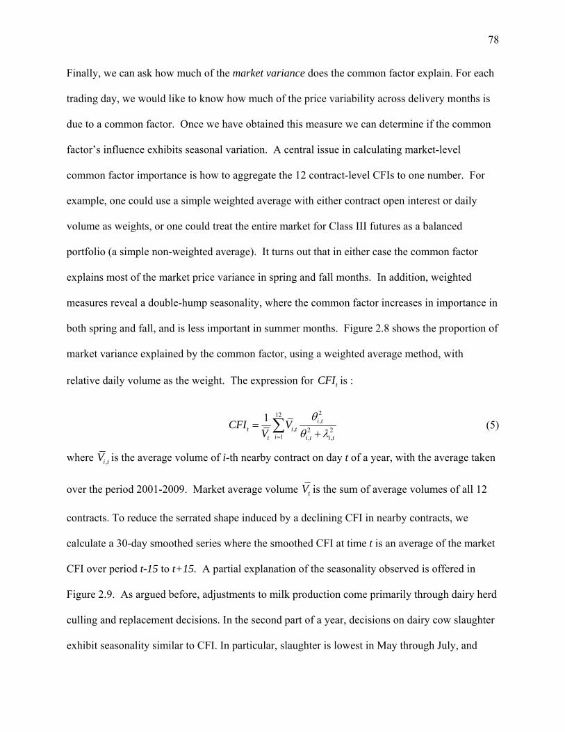
78
Finally, we can ask how much of the market variance does the common factor explain. For each
trading day, we would like to know how much of the price variability across delivery months is
due to a common factor. Once we have obtained this measure we can determine if the common
factor’s influence exhibits seasonal variation. A central issue in calculating market-level
common factor importance is how to aggregate the 12 contract-level CFIs to one number. For
example, one could use a simple weighted average with either contract open interest or daily
volume as weights, or one could treat the entire market for Class III futures as a balanced
portfolio (a simple non-weighted average). It turns out that in either case the common factor
explains most of the market price variance in spring and fall months. In addition, weighted
measures reveal a double-hump seasonality, where the common factor increases in importance in
both spring and fall, and is less important in summer months. Figure 2.8 shows the proportion of
market variance explained by the common factor, using a weighted average method, with
relative daily volume as the weight. The expression for tCFI is :
212,
, 2 21 , ,
1 i tt i t
it i t i t
CFI VV
(5)
where ,i tV is the average volume of i-th nearby contract on day t of a year, with the average taken
over the period 2001-2009. Market average volume tV is the sum of average volumes of all 12
contracts. To reduce the serrated shape induced by a declining CFI in nearby contracts, we
calculate a 30-day smoothed series where the smoothed CFI at time t is an average of the market
CFI over period t-15 to t+15. A partial explanation of the seasonality observed is offered in
Figure 2.9. As argued before, adjustments to milk production come primarily through dairy herd
culling and replacement decisions. In the second part of a year, decisions on dairy cow slaughter
exhibit seasonality similar to CFI. In particular, slaughter is lowest in May through July, and

79
reaches a peak in October and November. Seasonality of CFI influences may be partially
attributable to seasonality in the information flow regarding the future size of the dairy herd.
2.7. Conclusions
This paper describes the evolution of dairy futures markets, and explicitly examines the volatility
dynamics of Class III milk futures contracts. The design of this contract allows it to be used as a
hedging instrument for cheese products as well as fluid and manufacturing grade milk. Even
though Class III milk is itself a nonstorable commodity, the analysis reveals a rather important
overlap of information pertinent to futures for different maturities. This is attributed to the
capital structure of the dairy herd and the storability of some dairy products underpinning the
USDA formula for minimum Class III milk prices. Seasonal variation reveals that contracts
expiring in summer months much more closely resemble contracts on storable commodities like
corn, while contracts expiring in winter months are more influenced by idiosyncratic shocks.
There are two principal implications of this study for contract design and dairy policy. First, the
modest importance of a common factor for most contract months implies that contracts of
different maturities are poor substitutes in a risk management program, and product cross-
hedging may not be particularly effective either. Corn, a much deeper agricultural futures
contract in terms of volume traded, has only 5 contract months per year. However, even though
Class III futures often suffer from illiquidity, it is likely optimal to have separate contracts for all
12 months in the year.
An important question for policy makers concerns the ability of futures markets to substitute for
binding milk price supports as an instrument for enhancing cash price stability. As shown in the
spectral analysis in Appendix 1, a major contributor to cash milk price variance comes from a
cycle whose period is about 3 years. While Class III futures are listed for up to 24 months ahead,
80
contracts with more than 260 trading days to maturity do not generate any significant trading
interest. The ability of futures markets to dampen the low-frequency cash price oscillations
relies on two factors. The first is the degree to which farmers use futures as forecasts of milk
prices in later years in making dairy herd replacement decisions. Decisions regarding the dairy
herd are investment decisions with a relevant planning horizon of 3-5 years, and forecasts of next
year’s prices will guide their investment decisions only if they believe price expectations for
longer horizons are accurate, and that their individual production decisions will not impact future
prices. If the first condition is satisfied, we would still need farmers to have confidence that
futures prices carry economically meaningful information over the horizon used in investment
decisions. Futures prices are likely unbiased predictors of future cash milk prices, but the average
absolute prediction errors for horizons longer than 60 days is rather high. For example, at 9.5
months to maturity – the duration of a cow’s gestation period - futures price prediction errors are
on average 28%. That means that if the futures price is $16.00 per hundredweight, the final price
would be expected to be between $20.50 per cwt. (which would render milk production rather
profitable), and $12.00, which is low enough to initiate countercyclical price supports (i.e. MILC
payments). In face of such high prediction uncertainty, it is questionable whether futures serve a
major role in coordinating expectations to a degree that meaningfully reduces the amplitude of
the boom-bust cycle.
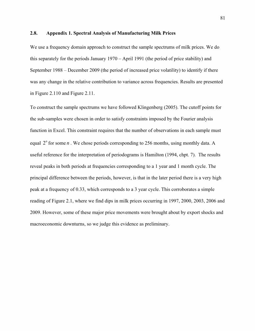
81
2.8. Appendix 1. Spectral Analysis of Manufacturing Milk Prices
We use a frequency domain approach to construct the sample spectrums of milk prices. We do
this separately for the periods January 1970 – April 1991 (the period of price stability) and
September 1988 – December 2009 (the period of increased price volatility) to identify if there
was any change in the relative contribution to variance across frequencies. Results are presented
in Figure 2. 110 and Figure 2.11.
To construct the sample spectrums we have followed Klingenberg (2005). The cutoff points for
the sub-samples were chosen in order to satisfy constraints imposed by the Fourier analysis
function in Excel. This constraint requires that the number of observations in each sample must
equal 2n for some n . We chose periods corresponding to 256 months, using monthly data. A
useful reference for the interpretation of periodograms is Hamilton (1994, chpt. 7). The results
reveal peaks in both periods at frequencies corresponding to a 1 year and 1 month cycle. The
principal difference between the periods, however, is that in the later period there is a very high
peak at a frequency of 0.33, which corresponds to a 3 year cycle. This corroborates a simple
reading of Figure 2.1, where we find dips in milk prices occurring in 1997, 2000, 2003, 2006 and
2009. However, some of these major price movements were brought about by export shocks and
macroeconomic downturns, so we judge this evidence as preliminary.
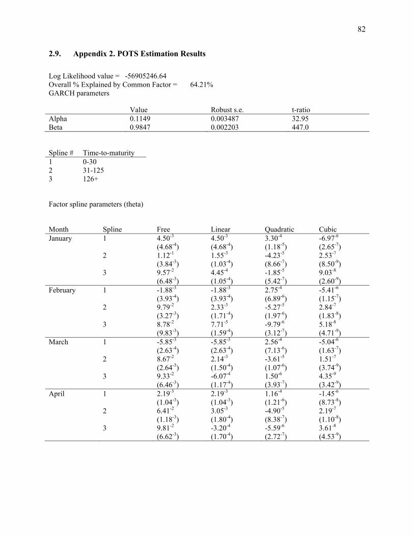
82
2.9. Appendix 2. POTS Estimation Results
Log Likelihood value = -56905246.64 Overall % Explained by Common Factor = 64.21% GARCH parameters
Value Robust s.e. t-ratio Alpha 0.1149 0.003487 32.95 Beta 0.9847 0.002203 447.0
Spline # Time-to-maturity 1 0-30 2 31-125 3 126+
Factor spline parameters (theta)
Month Spline Free Linear Quadratic Cubic January 1 4.50-3 4.50-3 3.30-4 -6.97-6 (4.68-4) (4.68-4) (1.18-5) (2.65-7) 2 1.12-1 1.55-3 -4.23-5 2.53-7 (3.84-3) (1.03-4) (8.66-7) (8.50-9) 3 9.57-2 4.45-4 -1.85-5 9.03-8 (6.48-3) (1.05-4) (5.42-7) (2.60-9) February 1 -1.88-3 -1.88-3 2.75-4 -5.41-6 (3.93-4) (3.93-4) (6.89-6) (1.15-7) 2 9.79-2 2.33-3 -5.27-5 2.84-7 (3.27-3) (1.71-4) (1.97-6) (1.83-8) 3 8.78-2 7.71-5 -9.79-6 5.18-8 (9.83-3) (1.59-4) (3.12-7) (4.71-9) March 1 -5.85-3 -5.85-3 2.56-4 -5.04-6 (2.63-4) (2.63-4) (7.13-6) (1.63-7) 2 8.67-2 2.14-3 -3.61-5 1.51-7 (2.64-3) (1.50-4) (1.07-6) (3.74-9) 3 9.33-2 -6.07-4 1.50-6 4.35-9 (6.46-3) (1.17-4) (3.93-7) (3.42-9) April 1 2.19-3 2.19-3 1.16-4 -1.45-6 (1.04-3) (1.04-3) (1.21-6) (8.73-8) 2 6.41-2 3.05-3 -4.90-5 2.19-7 (1.18-3) (1.80-4) (8.38-7) (1.10-8) 3 9.81-2 -3.20-4 -5.59-6 3.61-8 (6.62-3) (1.70-4) (2.72-7) (4.53-9)

83
Factor-spline parameters (theta) – cont’d. Month Spline Free Linear Quadratic Cubic May 1 2.71-3 2.71-3 3.32-4 -7.39-6 (2.81-4) (2.81-4) (7.86-6) (1.87-7) 2 1.01-1 5.84-4 -5.63-6 -4.03-9 (2.17-3) (5.49-5) (2.14-7) (4.64-10) 3 1.02-1 -6.09-4 -8.83-7 1.65-8 (4.32-3) (4.19-5) (7.78-7) (3.63-9) June 1 -6.23-3 -6.23-3 5.42-4 -1.22-5 (3.16-4) (3.16-4) (2.03-5) (5.10-7) 2 1.53-1 7.08-4 -3.37-5 2.14-7 (4.71-3) (1.69-4) (8.91-7) (1.40-8) 3 9.94-2 1.58-4 -1.20-5 5.83-8 (5.92-3) (1.58-4) (7.06-7) (6.03-9) July 1 1.15-3 1.15-3 4.95-4 -1.02-5 (3.13-4) (3.13-4) (1.39-5) (4.15-7) 2 1.68-1 2.92-3 -8.07-5 4.50-7 (2.44-3) (2.99-4) (2.07-6) (2.25-8) 3 1.03-1 -1.30-4 -7.11-6 4.03-8 (1.09-2) (2.40-4) (3.54-7) (3.46-9) August 1 -1.33-2 -1.33-2 2.98-4 -4.32-6 (6.76-4) (6.76-4) (6.11-6) (2.39-7) 2 1.32-1 6.41-3 -1.32-4 6.64-7 (2.49-3) (3.00-4) (3.72-6) (1.26-8) 3 1.16-1 -6.36-4 -1.86-7 1.37-8 (7.35-3) (1.40-4) (6.47-7) (1.57-9) September 1 -1.79-3 -1.79-3 1.35-4 -5.84-7 (9.25-4) (9.25-4) (3.62-6) (4.13-8) 2 9.72-2 6.33-3 -1.04-4 4.54-7 (1.87-3) (1.40-4) (3.54-6) (2.40-8) 3 1.44-1 -1.17-3 3.65-6 4.41-9 (7.20-3) (1.05-4) (3.14-7) (2.64-9) October 1 -2.61-3 -2.61-3 2.75-4 -4.98-6 (3.60-4) (3.60-4) (8.19-6) (8.86-8) 2 1.07-1 3.36-3 -4.45-5 1.45-7 (7.47-3) (5.76-4) (4.48-6) (3.32-9) 3 1.47-1 -1.19-3 3.17-6 7.68-9 (2.00-2) (3.37-4) (2.70-7) (6.81-9) November 1 1.67-4 1.67-4 2.49-4 -4.89-6 (4.91-4) (4.91-4) (2.86-6) (5.41-8) 2 9.04-2 2.12-3 -2.39-5 7.01-8 (1.58-3) (6.66-5) (6.19-7) (2.28-9) 3 1.35-1 -5.45-4 -7.03-6 4.75-8 (4.41-3) (3.66-5) (3.81-7) (2.21-9) December 1 -5.29-3 -5.29-3 5.17-4 -1.20-5 (3.81-4) (3.81-4) (1.16-5) (2.77-7) 2 1.36-1 -3.37-4 -2.86-7 2.80-8 (2.64-3) (4.04-5) (2.47-8) (4.40-10) 3 1.26-1 3.81-4 -2.06-5 1.03-7 (2.79-3) (4.03-5) (5.01-7) (2.89-9)
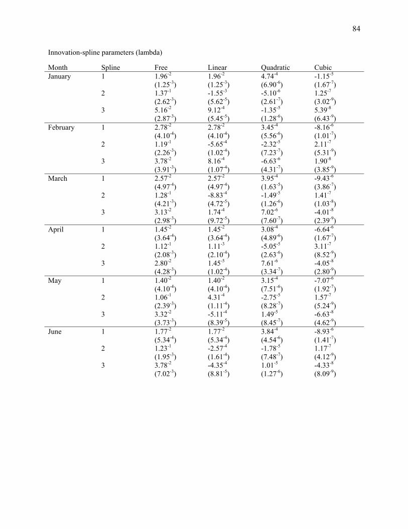
84
Innovation-spline parameters (lambda)
Month Spline Free Linear Quadratic Cubic January 1 1.96-2 1.96-2 4.74-4 -1.15-5 (1.25-3) (1.25-3) (6.90-6) (1.67-7) 2 1.37-1 -1.55-3 -5.10-6 1.25-7 (2.62-3) (5.62-5) (2.61-7) (3.02-9) 3 5.16-2 9.12-4 -1.35-5 5.39-8 (2.87-3) (5.45-5) (1.28-6) (6.43-9) February 1 2.78-2 2.78-2 3.45-4 -8.16-6 (4.10-4) (4.10-4) (5.56-6) (1.01-7) 2 1.19-1 -5.65-4 -2.32-5 2.11-7 (2.26-3) (1.02-4) (7.23-7) (5.31-9) 3 3.78-2 8.16-4 -6.63-6 1.90-8 (3.91-3) (1.07-4) (4.31-7) (3.85-9) March 1 2.57-2 2.57-2 3.95-4 -9.43-6 (4.97-4) (4.97-4) (1.63-5) (3.86-7) 2 1.28-1 -8.83-4 -1.49-5 1.41-7 (4.21-3) (4.72-5) (1.26-6) (1.03-8) 3 3.13-2 1.74-4 7.02-6 -4.01-8 (2.98-3) (9.72-5) (7.60-7) (2.39-9) April 1 1.45-2 1.45-2 3.08-4 -6.64-6 (3.64-4) (3.64-4) (4.89-6) (1.67-7) 2 1.12-1 1.11-3 -5.05-5 3.11-7 (2.08-3) (2.10-4) (2.63-6) (8.52-9) 3 2.80-2 1.45-5 7.61-6 -4.05-8 (4.28-3) (1.02-4) (3.34-7) (2.80-9) May 1 1.40-2 1.40-2 3.15-4 -7.07-6 (4.10-4) (4.10-4) (7.51-6) (1.92-7) 2 1.06-1 4.31-4 -2.75-5 1.57-7 (2.39-3) (1.11-4) (8.28-7) (5.24-9) 3 3.32-2 -5.11-4 1.49-5 -6.63-8 (3.73-3) (8.39-5) (8.45-7) (4.62-9) June 1 1.77-2 1.77-2 3.84-4 -8.93-6 (5.34-4) (5.34-4) (4.54-6) (1.41-7) 2 1.23-1 -2.57-4 -1.78-5 1.17-7 (1.95-3) (1.61-4) (7.48-7) (4.12-9) 3 3.78-2 -4.35-4 1.01-5 -4.33-8 (7.02-3) (8.81-5) (1.27-6) (8.09-9)
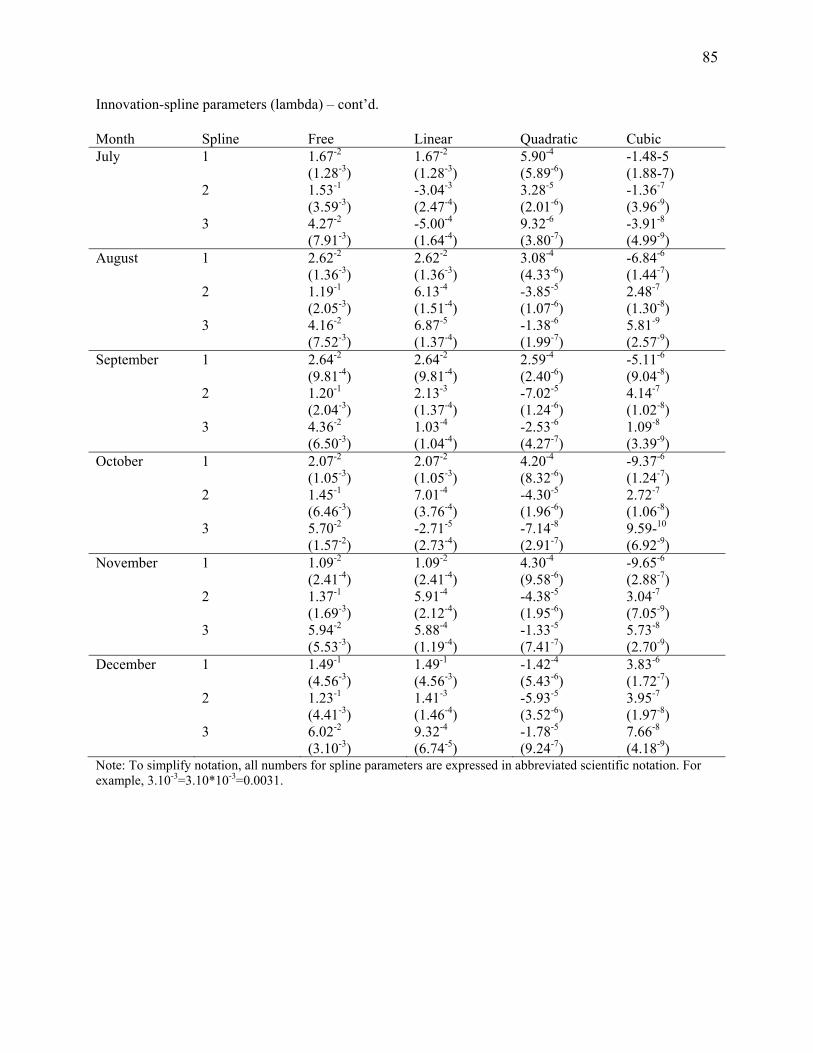
85
Innovation-spline parameters (lambda) – cont’d.
Note: To simplify notation, all numbers for spline parameters are expressed in abbreviated scientific notation. For example, 3.10-3=3.10*10-3=0.0031.
Month Spline Free Linear Quadratic Cubic July 1 1.67-2 1.67-2 5.90-4 -1.48-5 (1.28-3) (1.28-3) (5.89-6) (1.88-7) 2 1.53-1 -3.04-3 3.28-5 -1.36-7 (3.59-3) (2.47-4) (2.01-6) (3.96-9) 3 4.27-2 -5.00-4 9.32-6 -3.91-8 (7.91-3) (1.64-4) (3.80-7) (4.99-9) August 1 2.62-2 2.62-2 3.08-4 -6.84-6 (1.36-3) (1.36-3) (4.33-6) (1.44-7) 2 1.19-1 6.13-4 -3.85-5 2.48-7 (2.05-3) (1.51-4) (1.07-6) (1.30-8) 3 4.16-2 6.87-5 -1.38-6 5.81-9 (7.52-3) (1.37-4) (1.99-7) (2.57-9) September 1 2.64-2 2.64-2 2.59-4 -5.11-6 (9.81-4) (9.81-4) (2.40-6) (9.04-8) 2 1.20-1 2.13-3 -7.02-5 4.14-7 (2.04-3) (1.37-4) (1.24-6) (1.02-8) 3 4.36-2 1.03-4 -2.53-6 1.09-8 (6.50-3) (1.04-4) (4.27-7) (3.39-9) October 1 2.07-2 2.07-2 4.20-4 -9.37-6 (1.05-3) (1.05-3) (8.32-6) (1.24-7) 2 1.45-1 7.01-4 -4.30-5 2.72-7 (6.46-3) (3.76-4) (1.96-6) (1.06-8) 3 5.70-2 -2.71-5 -7.14-8 9.59-10 (1.57-2) (2.73-4) (2.91-7) (6.92-9) November 1 1.09-2 1.09-2 4.30-4 -9.65-6 (2.41-4) (2.41-4) (9.58-6) (2.88-7) 2 1.37-1 5.91-4 -4.38-5 3.04-7 (1.69-3) (2.12-4) (1.95-6) (7.05-9) 3 5.94-2 5.88-4 -1.33-5 5.73-8 (5.53-3) (1.19-4) (7.41-7) (2.70-9) December 1 1.49-1 1.49-1 -1.42-4 3.83-6 (4.56-3) (4.56-3) (5.43-6) (1.72-7) 2 1.23-1 1.41-3 -5.93-5 3.95-7 (4.41-3) (1.46-4) (3.52-6) (1.97-8) 3 6.02-2 9.32-4 -1.78-5 7.66-8 (3.10-3) (6.74-5) (9.24-7) (4.18-9)
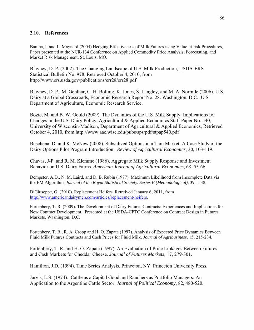
86
2.10. References
Bamba, I. and L. Maynard (2004) Hedging Effectiveness of Milk Futures using Value-at-risk Procedures, Paper presented at the NCR-134 Conference on Applied Commodity Price Analysis, Forecasting, and Market Risk Management, St. Louis, MO.
Blayney, D. P. (2002). The Changing Landscape of U.S. Milk Production, USDA-ERS Statistical Bulletin No. 978. Retrieved October 4, 2010, from http://www.ers.usda.gov/publications/err28/err28.pdf
Blayney, D. P., M. Gehlhar, C. H. Bolling, K. Jones, S. Langley, and M. A. Normile (2006). U.S. Dairy at a Global Crossroads, Economic Research Report No. 28. Washington, D.C.: U.S. Department of Agriculture, Economic Research Service.
Bozic, M. and B. W. Gould (2009). The Dynamics of the U.S. Milk Supply: Implications for Changes in the U.S. Dairy Policy, Agricultural & Applied Economics Staff Paper No. 540, University of Wisconsin-Madison, Department of Agricultural & Applied Economics, Retrieved October 4, 2010, from http://www.aae.wisc.edu/pubs/sps/pdf/stpap540.pdf
Buschena, D. and K. McNew (2008). Subsidized Options in a Thin Market: A Case Study of the Dairy Options Pilot Program Introduction. Review of Agricultural Economics, 30, 103-119.
Chavas, J-P. and R. M. Klemme (1986). Aggregate Milk Supply Response and Investment Behavior on U.S. Dairy Farms. American Journal of Agricultural Economics, 68, 55-66.
Dempster, A.D., N. M. Laird, and D. B. Rubin (1977). Maximum Likelihood from Incomplete Data via the EM Algorithm. Journal of the Royal Statistical Society. Series B (Methodological), 39, 1-38.
DiGiuseppe, G. (2010). Replacement Heifers. Retreived January 6, 2011, from http://www.americandairymen.com/articles/replacement-heifers.
Fortenbery, T. R. (2009). The Development of Dairy Futures Contracts: Experiences and Implications for New Contract Development. Presented at the USDA-CFTC Conference on Contract Design in Futures Markets, Washington, D.C.
Fortenbery, T. R., R. A. Cropp and H. O. Zapata (1997). Analysis of Expected Price Dynamics Between Fluid Milk Futures Contracts and Cash Prices for Fluid Milk. Journal of Agribusiness, 15, 215-234.
Fortenbery, T. R. and H. O. Zapata (1997). An Evaluation of Price Linkages Between Futures and Cash Markets for Cheddar Cheese. Journal of Futures Markets, 17, 279-301.
Hamilton, J.D. (1994). Time Series Analysis. Princeton, NY: Princeton University Press.
Jarvis, L.S. (1974). Cattle as a Capital Good and Ranchers as Portfolio Managers: An Application to the Argentine Cattle Sector. Journal of Political Economy, 82, 480-520.
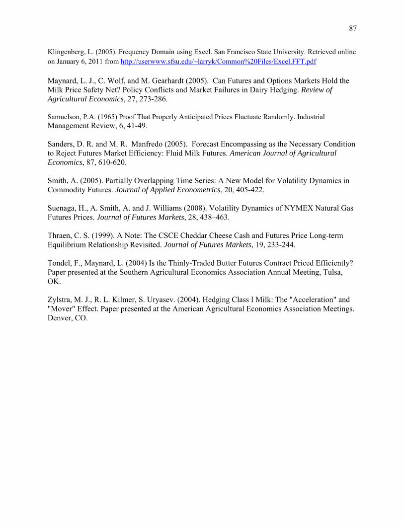
87
Klingenberg, L. (2005). Frequency Domain using Excel. San Francisco State University. Retrieved online on January 6, 2011 from http://userwww.sfsu.edu/~larryk/Common%20Files/Excel.FFT.pdf
Maynard, L. J., C. Wolf, and M. Gearhardt (2005). Can Futures and Options Markets Hold the Milk Price Safety Net? Policy Conflicts and Market Failures in Dairy Hedging. Review of Agricultural Economics, 27, 273-286.
Samuelson, P.A. (1965) Proof That Properly Anticipated Prices Fluctuate Randomly. Industrial Management Review, 6, 41-49.
Sanders, D. R. and M. R. Manfredo (2005). Forecast Encompassing as the Necessary Condition to Reject Futures Market Efficiency: Fluid Milk Futures. American Journal of Agricultural Economics, 87, 610-620.
Smith, A. (2005). Partially Overlapping Time Series: A New Model for Volatility Dynamics in Commodity Futures. Journal of Applied Econometrics, 20, 405-422.
Suenaga, H., A. Smith, A. and J. Williams (2008). Volatility Dynamics of NYMEX Natural Gas Futures Prices. Journal of Futures Markets, 28, 438–463.
Thraen, C. S. (1999). A Note: The CSCE Cheddar Cheese Cash and Futures Price Long-term Equilibrium Relationship Revisited. Journal of Futures Markets, 19, 233-244.
Tondel, F., Maynard, L. (2004) Is the Thinly-Traded Butter Futures Contract Priced Efficiently? Paper presented at the Southern Agricultural Economics Association Annual Meeting, Tulsa, OK.
Zylstra, M. J., R. L. Kilmer, S. Uryasev. (2004). Hedging Class I Milk: The "Acceleration" and "Mover" Effect. Paper presented at the American Agricultural Economics Association Meetings. Denver, CO.
88
Figure 2.1. Manufacturing Milk Price: 1970-2009

89
Figure 1.2. Class III Milk futures - Partially Overlapping Time Series vs. “Nearby” Series
Note: This figure illustrates the difference between the standard analysis of futures prices and POTS model, as applied to the Class III milk futures. Contracts are denoted with indexes (e.g. 2004-Jan: 133, 2004-Feb: 134, …). Dashed line represents the period when a particular Class III contract traded. Bold line represents data used to create continuous 1st nearby series. Unlike the standard analysis of futures prices that use only data segments represented with bolded line, POTS model utilizes all traded data for all contracts (both dashed and bold line segments).

90
Figure 2.3. Class III Milk Futures: Open Interest and Nearby Price 2000-2009.
91
Figure 2.4. Realized Prediction Errors of Class III Milk Futures Prices.
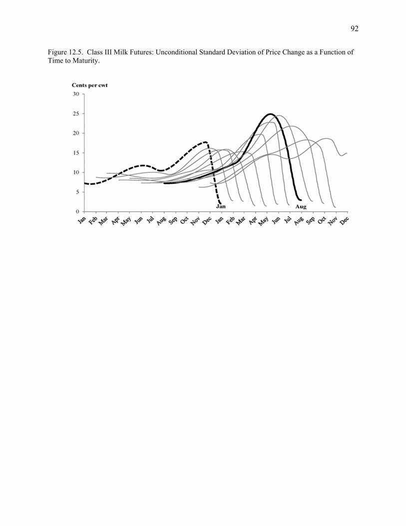
92
Figure 12.5. Class III Milk Futures: Unconditional Standard Deviation of Price Change as a Function of Time to Maturity.
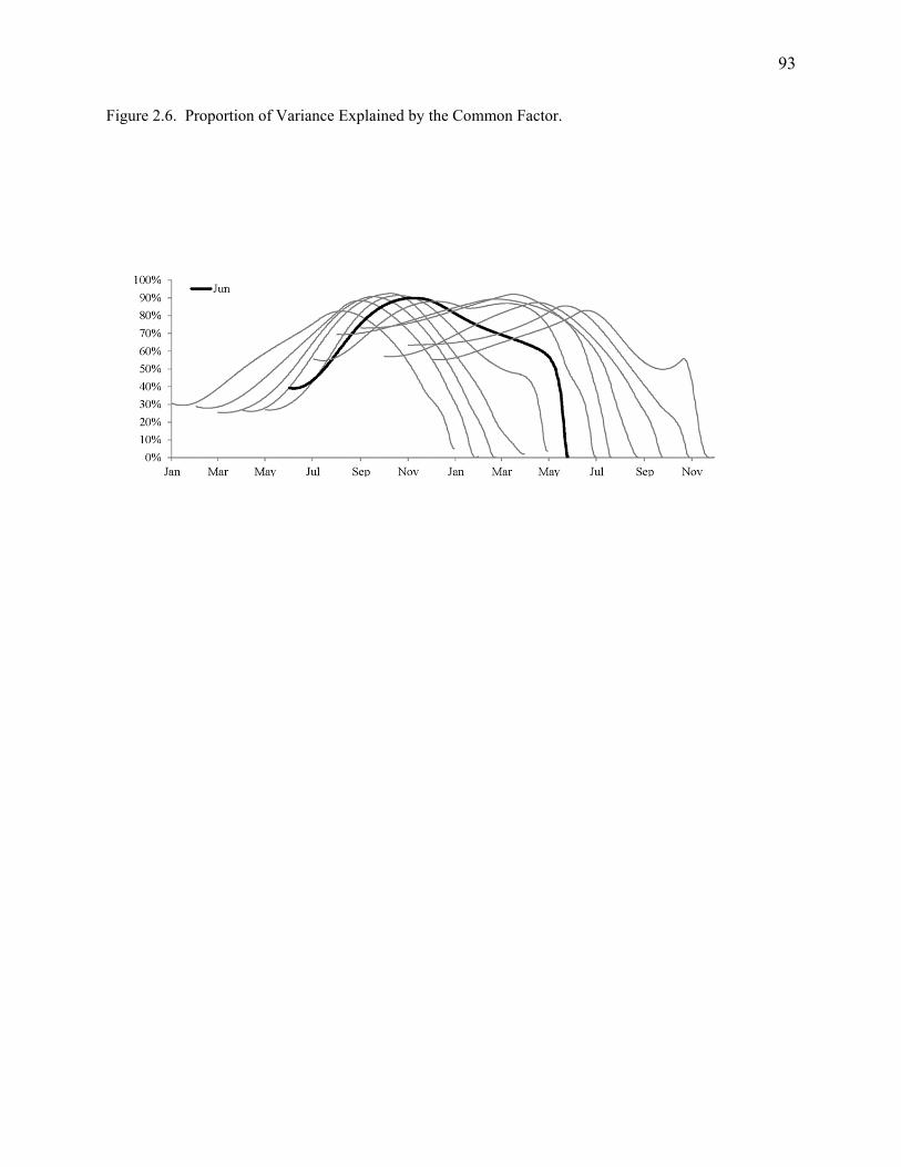
93
Figure 2.6. Proportion of Variance Explained by the Common Factor.

94
Figure 2.7. Common Factor Importance for Class III Milk Futures.
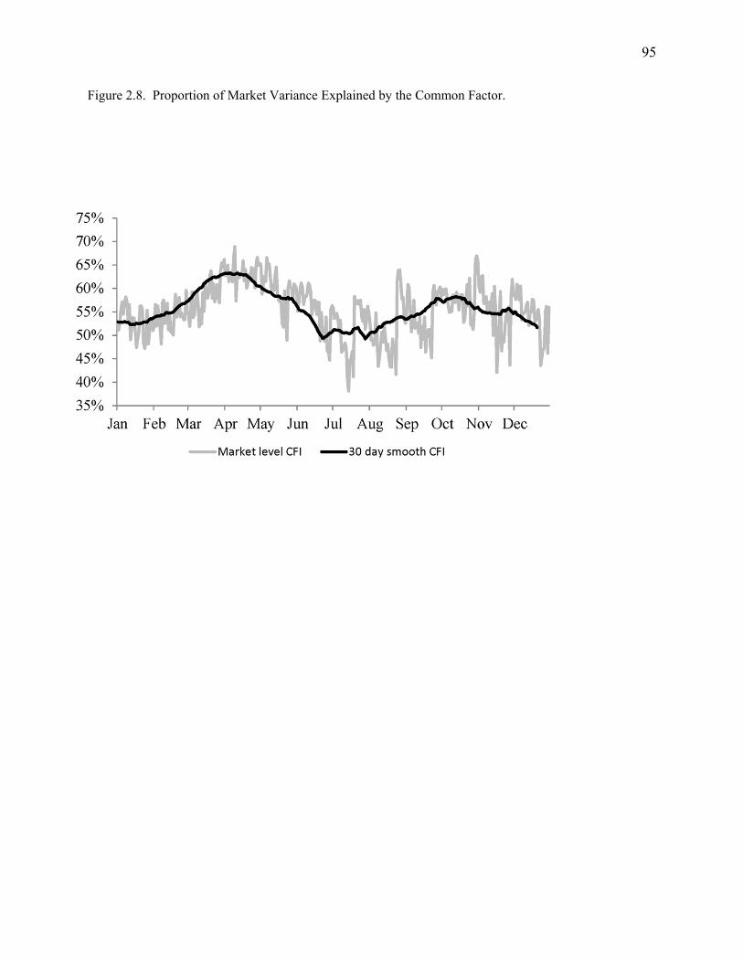
95
Figure 2.8. Proportion of Market Variance Explained by the Common Factor.
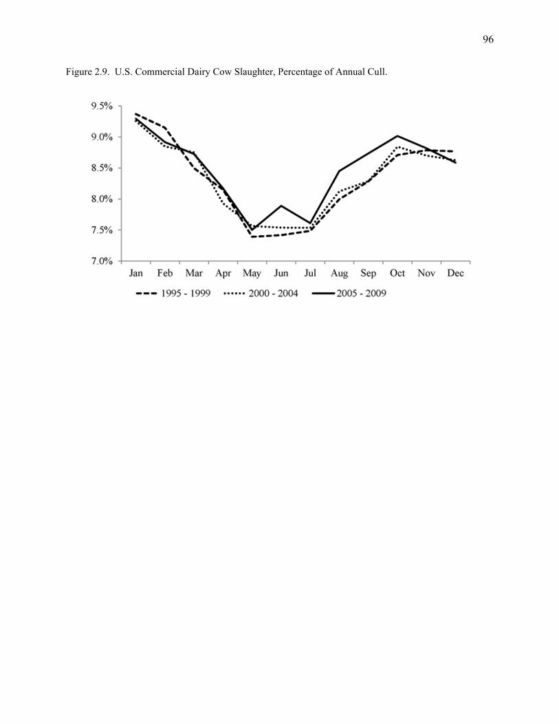
96
Figure 2.9. U.S. Commercial Dairy Cow Slaughter, Percentage of Annual Cull.
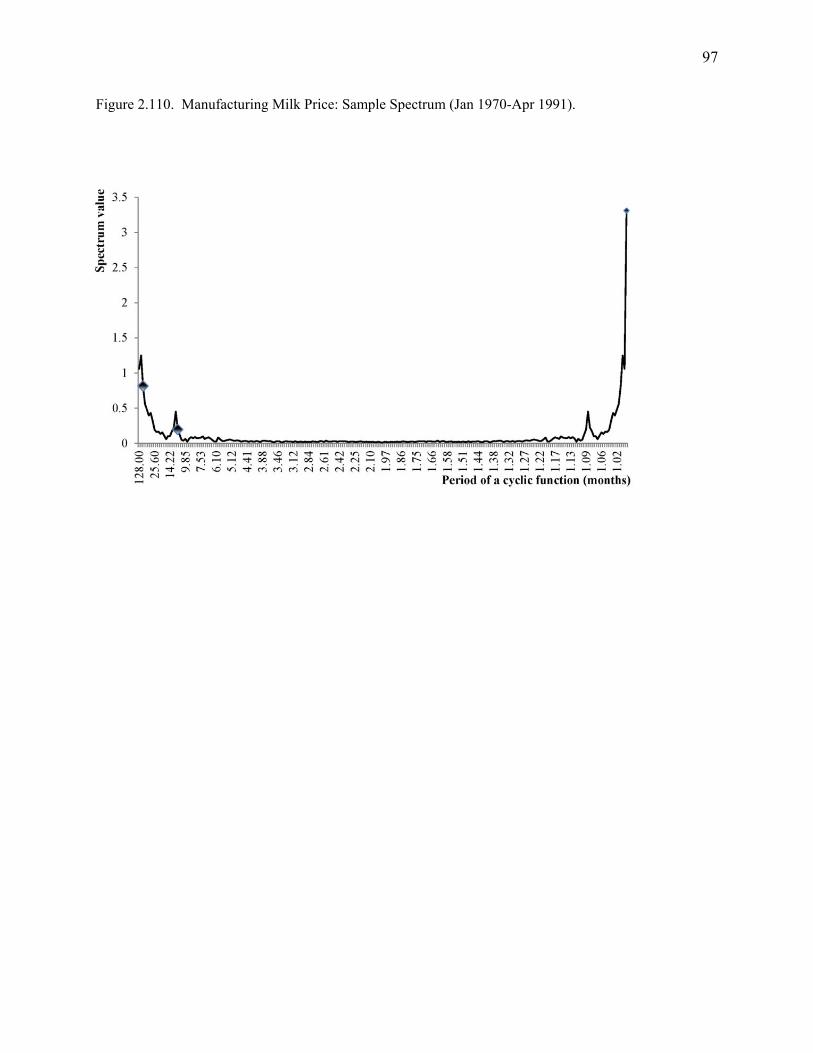
97
Figure 2. 110. Manufacturing Milk Price: Sample Spectrum (Jan 1970-Apr 1991).
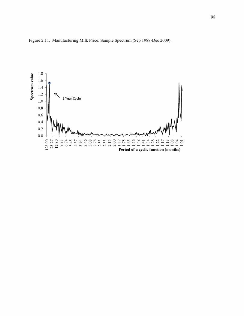
98
Figure 2.11. Manufacturing Milk Price: Sample Spectrum (Sep 1988-Dec 2009).
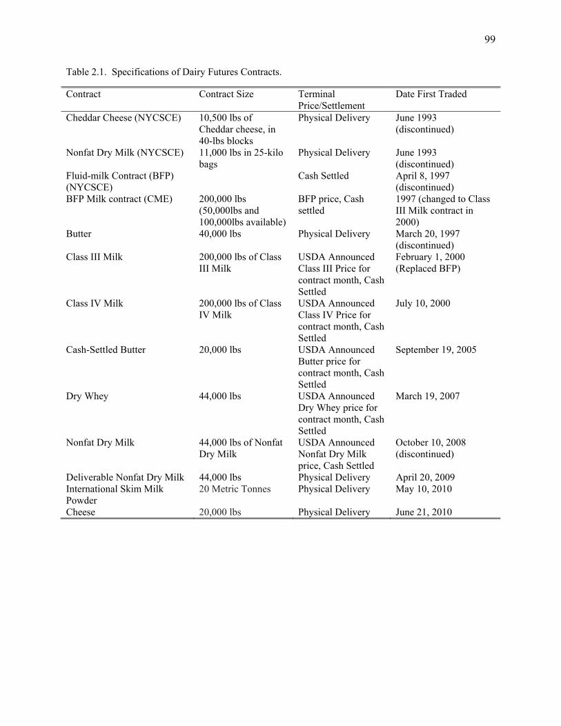
99
Table 2.1. Specifications of Dairy Futures Contracts.
Contract Contract Size Terminal Price/Settlement
Date First Traded
Cheddar Cheese (NYCSCE) 10,500 lbs of Cheddar cheese, in 40-lbs blocks
Physical Delivery June 1993 (discontinued)
Nonfat Dry Milk (NYCSCE) 11,000 lbs in 25-kilo bags
Physical Delivery June 1993 (discontinued)
Fluid-milk Contract (BFP) (NYCSCE)
Cash Settled April 8, 1997 (discontinued)
BFP Milk contract (CME) 200,000 lbs (50,000lbs and 100,000lbs available)
BFP price, Cash settled
1997 (changed to Class III Milk contract in 2000)
Butter 40,000 lbs Physical Delivery March 20, 1997 (discontinued)
Class III Milk 200,000 lbs of Class III Milk
USDA Announced Class III Price for contract month, Cash Settled
February 1, 2000 (Replaced BFP)
Class IV Milk 200,000 lbs of Class IV Milk
USDA Announced Class IV Price for contract month, Cash Settled
July 10, 2000
Cash-Settled Butter 20,000 lbs USDA Announced Butter price for contract month, Cash Settled
September 19, 2005
Dry Whey 44,000 lbs USDA Announced Dry Whey price for contract month, Cash Settled
March 19, 2007
Nonfat Dry Milk 44,000 lbs of Nonfat Dry Milk
USDA Announced Nonfat Dry Milk price, Cash Settled
October 10, 2008 (discontinued)
Deliverable Nonfat Dry Milk 44,000 lbs Physical Delivery April 20, 2009 International Skim Milk Powder
20 Metric Tonnes
Physical Delivery May 10, 2010
Cheese 20,000 lbs Physical Delivery June 21, 2010

100
Table 2.2. Dairy Prices: Correlations 2000-2009.
Class III Class IV Nonfat DryMilk Butter
Class IV 0.83 1 Nonfat Dry Milk 0.65 0.89 1 Butter 0.54 0.46 0.04 1 Dry Whey 0.54 0.64 0.71 0.14 Cheddar Cheese 0.95 0.78 Fluid Milk 0.97 0.90

101
Table 2.3. Determination of Manufacturing Grade Milk Price in Federal Milk Marketing Orders
Weekly average price and total sales volume Monthly weighted average price and cumulative sales
Commodity Oct 4, 2008 Oct 11, 2008 Oct 18, 2008 Oct 25, 2008 October 2008 40lbs cheddar cheese blocks
$1.9194 10,938,573 lbs
$1.9176 11,069,262 lbs
$1.8781 11,338,644 lbs
$1.8557 10,822,753 lbs
1.8927 44,169,232 lbs
500lbs cheddar cheese barrels†
$1.9253 9,180,226 lbs
$1.9124 9,027,224 lbs
$1.8612 9,758,321 lbs
$1.8752 9,548,341 lbs
$1.8928 37,514,112 lbs
Announced average cheddar cheese price††
$1.9065
Grade AA butter $1.6833 4,288,319
$1.7007 2,609,238
$1.7002 3,642,963
$1.7202 3,186,005
$1.6997
Dry Whey $0.2021 9,630,436
$0.1929 11,752,139
$0.1916 10,804,469
$0.1923 9,751,256
$0.1945
value of milk in cheddar cheese (9.64 X Cheese Price) $18.37 + value of milk in butter (0.42 X Butter Price) $0.72
+ value if milk in dry whey (5.86 X Dry Whey Price) $1.14 - value added by manufacturer through processing milk to dairy products (– 3.18) -$3.18
= Class III milk price $17.06
Note: † Adjusted to 38% moisture. †† 500lbs cheddar cheese barrels price increased by 3 cents prior to averaging.
101
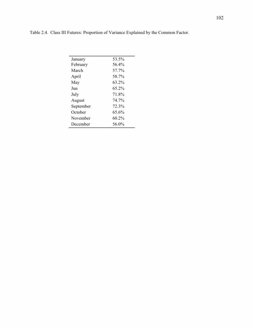
102
Table 2.4. Class III Futures: Proportion of Variance Explained by the Common Factor.
January 53.5% February 56.4% March 57.7% April 58.7% May 63.2% Jun 65.2% July 71.8% August 74.7% September 72.3% October 65.6% November 60.2% December 56.0%
103
3. Price Discovery, Volatility Spillovers and Adequacy of Speculation in Cheese Spot and
Futures Markets
ABSTRACT. The task of this essay is to examine price discovery, volatility spillovers and impacts of
speculation in the dairy sector. I have developed a method that allows for the calculation of implied
cheese futures prices for a period before cheese futures actually started trading. Evidence for periods
when cheese futures did trade suggests that utilized approximation methods perform very well.
Examining the time series properties of cheese cash and implied futures price I find that the unit root
hypothesis is strongly rejected for cash prices, while unit roots cannot be rejected for nearby futures
prices in the framework that carefully controls for rollovers. To explain this result, I built a model that
illustrates the time series properties of the nearby futures price series for a futures contract written on a
second-order stationary cash series and identified the mean-reverting nonlinear dynamics that will occur
at rollovers. Given the time series properties of the cash and futures series I propose an error-correction
model using spreads between cash and the second nearby futures instead of the cointegration vector. To
account for volatility dynamics I employ the GARCH-BEKK structure. I find that the flow of information
in the mean model is predominantly from futures to cash, while volatility spillovers are bidirectional. It is
possible that cash prices that include unfilled bid/offers react differently to increases in volatility in
futures prices than sales cash prices, though this result may not be robust and further research is needed to
identify if liquidity in the cash market is reduced with increase in conditional volatility of the futures
price. I propose an extension of the BEKK variance model that I refer to as GARCH-MEX. That model
does not restrict the sign of the additional regressors on the conditional variances, and can easily insure
positive-definiteness of the conditional covariance matrix. Utilizing that model to evaluate the impact of
speculation I find strong evidence against the hypothesis that excessive speculation is increasing the
conditional variance of futures prices. If anything, speculation may in fact be inadequate, and further
research with daily speculative positions and high-frequency futures prices is needed to identify the effect
of increased speculation on realized volatility of futures prices, bid-ask spread and magnitude of slippage.
JEL Codes: G13, Q13, C22 Keywords: implied cheese futures, unit root tests, volatility spillovers, speculation, GARCH-MEX
104
3.1. Introduction
There has been considerable interest in recent years concerning the overall performance of commodity futures markets, and the extent
to which futures activity has led to price instability in cash markets. Much of the recent work in futures/cash price relationships has
focused on the first moment of the price distribution and deep (large volume) markets (e.g. Irwin, Sanders and Merrin, 2009; Sanders,
Irwin and Merrin, 2010; Hamilton, 2009; Gilbert, 2010). However, equally important are the relationships between the second and
higher moments of futures/cash price distributions. Specifically, does price action in the futures market result in increased instability
(volatility) in cash markets? As noted by Witherspoon (1993), market composition may impact market stability, and, as noted by
Fortenbery and Zapata (2004), this may be more apparent in thin markets.
Dairy markets are unique for several reasons, not the least of which is the relative age of the futures markets for dairy. Dairy futures
markets have existed since 1993, but underwent continual re-design through the early 2000’s. The re-designs were in response to both
changes in dairy market structure, and changes in dairy policy. Early work on dairy suggested that there were problems with the
relationships between dairy futures and cash markets (Fortenbery and Zapata, 1997). In later work, it appeared that the issues had
resolved themselves (Fortenbery, Cropp and Zapata, 1997; Thraen 1999). However, recent price action has again called into question
the relationship between futures and cash markets for dairy, the impacts of technical innovation in the dairy sector on price
performance, and the role of public policy in promoting price stability. Past work on price performance is dated given recent changes
in both production and price policy.

105
This paper investigates price action and performance in dairy markets in several ways. First, the actual relationship between cash and
futures price is studied. Both futures and cash markets have undergone significant changes over the last ten years, and their
relationship to each other has not been examined recently. Futures changes include changes in futures contract design, delivery
specifications, and the actual dairy commodities traded. On the cash side, the closing of the Green Bay Cheese Exchange, its
replacement by a cash market in Chicago, and changes in both cash market structure and technology adoption in production may have
impacted the cash/futures relationships.
I open the essay with a brief review of literature examining the information flow between cash and futures markets and the impact of
speculators activity on both. In the second section, I describe the daily wholesale cash market for cheese as well as futures contracts
for cheese and other dairy futures. A technique for calculating ‘implied’ cheese futures price for the period before actual cheese
futures contract started trading is then discussed. Time series properties of cash and nearby futures cheese price are evaluated next.
The fourth section discusses in further detail the concepts of causality as they are commonly used in the applied econometrics
literature. An error-correction model with a GARCH-BEKK variance structure is then proposed as an appropriate analytical
framework given the results of unit root tests, followed by the discussion of empirical results. To examine the influence of speculators
on price volatility new GARCH model is proposed that nests BEKK variance structure while allowing flexibility in the direction of
impact of additional regressors included in the variance model. I apply this model to evaluate the adequacy of speculation in the Class
III milk futures. Paper concludes with policy implications and suggestions for further research.
106
3.2. Literature Review
Do futures markets, by facilitating speculation, increase cash price volatility? Early work by Working (1960, Feb) in onion futures
demonstrated that speculative support at harvest time reduced both seasonal price range and price adjustments at the end of the
marketing year, as needed adjustments were better anticipated and incorporated in prices earlier. Gray (1963) extended Working’s
analysis to include seasonal patterns in onion cash prices after the trade in onion futures was prohibited. He found that pronounced
seasonality in cash prices, reduced during the years of intense futures trading, had returned after onion futures were discontinued.
In addition to reductions in seasonality and earlier anticipation of adjustments needed at the end of a marketing year, futures may
reduce year-to-year price fluctuations. Whereas the first two effects are mediated through the impacts of futures prices on storage
decisions, the last effect will be present if the futures prices are perceived as reliable guides to production planning, and farmers
engage in what Working (1962) calls anticipatory hedging.
Powers (1970) investigated live beef and pork belly markets around the time futures contracts were first introduced for these
commodities. He modeled weekly cash prices as the sum of two components assumed to be uncorrelated: the systematic component
associated with fundamental economic conditions and the error or random component which represents noise and disturbance in the
price system. He employed a variate difference method to separate systematic and random components, and then calculated the
variance of the random part separately for four year periods before and after the introduction of futures markets. For both commodities
he analyzes, he found that the variance of the noise decreased after futures contracts were introduced, but offered no statistical
107
evidence that reduction can be attributed to information services performed by the futures market. Taylor and Leuthold (1974)
examined the impact of new futures market on the variance of average annual, monthly and weekly of livestock cash prices, and found
that while weekly and monthly variances decreased, the effect on annual variability was not statistically significant. They conjecture
that the differential effect of futures market introduction on different frequencies may be due to a contract design, as livestock
contracts at that time did not trade for horizons sufficiently long to influence the behavior of livestock breeders, given the long
reproductive cycle of cattle. Brorsen, Oellerman and Farris (1989) extended the analysis to daily live cattle cash price variability. In
their theoretical model, faster information assimilation was enabled by the introduction of a futures market, and the transmission of
that information to the cash market resulted in increased daily variability in cash prices, and a reduction in cash price autocorrelation.
Empirical analysis encompassing periods before and after live cattle futures were introduced confirmed their hypotheses. They
concluded that live cattle futures improved the cash market efficiency, but increased short-term price risk.
Cox (1976) proposed that introducing of a futures market may attract a new set of traders who acquire and process information in
order to predict future cash prices, but do not handle the physical commodity. Speculators participating in the futures market may be
more informed about the future supply and demand conditions than commercial parties. If that is the case, the addition of a futures
market will enable the cash market to more quickly absorb the most recent information. The testable hypotheses emerging from Cox’s
work are twofold. First, the addition of a futures market will change the time series properties of the cash prices, with autoregressive
components in cash price process fading in importance. In addition, expected prices will be more reliable predictors of future cash
prices, i.e. the variance of the price-forecast error will decrease.
108
Turnovsky (1983) adds to the literature by showing that in the case where producers are risk averse, introduction of a futures market
will affect not only the information set based on which the expectation of future spot prices are made, but also the slopes of the supply
and inventory demand functions as they depend on the degree of price stability. He found that under a wide range of behavioral
assumptions the futures market reduces both cash price volatility and long run average spot price.
Newbery (1987) extended Turnovsky’s basic idea that futures markets can insure against risk, and thus increase the supply of
otherwise risky activities. He built a model in which farmers must choose among two competing plant breeds, one that produces less
output but with no uncertainty and another that is risky, but produces higher average yield. Once hedging with futures becomes
available farmers may trade some price risk for increased production risk. If a sufficient number of producers exhibited such behavior,
then the volatility of cash price may in fact increase. In his study the futures market did not destabilize cash price through speculative
activities but through the impact on producer decision-making.
The price discovery function of the futures market is the ability of the futures prices to quickly absorb new price-relevant information
and transmit it through to the cash prices. Price discovery has been the subject of a vast empirical literature, and some examples
include Garbade and Silber (1983), Oellerman and Farris (1985), Schroeder and Goodwin (1991), Fortenbery and Zapata (1993,
1997), Zapata and Fortenbery (1996), and Yang and Bessler (2001). In early work, dynamic models in either price levels or
differenced prices were utilized. With development of time series methods that can appropriately address nonstationarity of prices,
researchers have started using co-integration models to analyze price discovery. Of particular interest for the present study are articles
analyzing the price discovery in thin markets. In such settings, Brockman and Tse (1995), Fortenbery and Zapata (1997), Mattos and
109
Garcia (2006) and Ivanov and Cho (2011) find that price discovery can be hampered by the lack of liquidity or institutional
constraints. This is manifested as either lack of cointegrating relationship between cash and futures market or lower information share
of futures market in the price discovery process.
Impact of speculation on price levels and volatility dynamics has been recently investigated in several papers. For example, in his
testimony before the U.S. Senate, Masters (2008) argued that institutional investors are among the major factors affecting
commodities prices, and Gilbert (2010) argues that index futures investment was the principal channel through which monetary and
financial activity have affected food prices in the second half of 2000s. However, Irwin, Sanders and Merrin (2009) argue that bubbles
in futures prices are not likely, and find that speculative positions do not Granger cause futures price changes. Earlier work by
Streeter and Tomek (1992) finds that volatility of soybeans futures decreases as Working’s T index of speculation increases. Du, Yu
and Hayes (2011) find a positive impact of speculation on crude oil price volatility. Using more detailed data, Brunetti and
Büyükşahin (2009) and Brunetti, Büyükşahin and Harris (2011) find that increased speculative activity does not destabilize financial
markets, and in fact predicts lower realized volatility in crude oil and other markets they analyze. However, Tang and Xiong (2010)
find that futures prices of different commodities in the US became increasingly correlated with each other and this trend was
significantly more pronounced for commodities in the two popular GSCI and DJ-UBS commodity indices. Büyükşahin and Robe
(2011) note that correlations between the returns on commodity and on equity indices increase significantly amid greater activity by
speculators in general and one type of traders in particular – hedge funds. These results may indicate that while speculators overall
help increase market liquidity, they increase the sensitivity of commodity prices to macroeconomic shocks.

110
3.3. Data
In this paper, we are interested in evaluating information flows between spot and futures markets in the dairy sector. While we are
ultimately interested in price discovery for milk price, there is in fact no national spot market for fluid milk. Given that the fluid milk
prices are linked to the prices of milk used in cheese production, the second best approach to investigating cash-futures relations
seems to be to look at the cash and futures markets for cheese. This section describes the aspects of the milk pricing environment in
the U.S. that are relevant to my research question.
Pricing of milk in the U.S. is highly regulated under Federal Milk Marketing Orders (FMMO). Three main objectives of the FMMOs
are: 1) insuring market price stability, 2) preventing processors from exercising market power over milk producers and 3) insuring
adequate supply and orderly marketing of fluid milk.
The primary instrument FMMOs use to achieve these objectives is to set minimum prices that handlers of Grade A milk must pay to
farmers. The fundamental principle currently used to determine minimum milk price is measure the value of milk as a function of milk
ingredients that have desirable nutritional qualities: milk protein, butterfat, and milk solids (lactose, whey proteins, minerals, lactic
acid).
Values of the principal milk components are inferred from derived dairy products like cheese, butter, dry whey and non-fat dry milk.
Finally, in order to calculate a minimum price of milk, a standard composition of milk in terms of percentages of each ingredient is
assumed. In particular, the standard used by the USDA assumes that milk used for the production of cheese consists of 3.5% butterfat,

111
2.99% protein and 5.69% other solids. The USDA differentiates between milk used for cheese production and milk used in production
of dry products. The former is referred to as Class III milk, and the latter Class IV milk. Similarly, milk used for fluid consumption is
termed Class I milk, and its minimum price exceeds the price of manufacturing milk. For milk produced for consumption, the
‘ingredient’ that carries the additional value is the location of marketing.
The flowchart in Figure 3.1 presents the procedure the USDA uses to arrive at the Class III and Class IV manufacturing milk prices.
First, major producers of butter, dry whey, nonfat dry milk and cheese are surveyed weekly. Monthly averages of these prices, with
weeks weighted by volume, are used to infer the average monthly price of the ingredients. In particular, let BtP be the average surveyed
price of butter in month t . Then the value of butterfat is calculated as
B B Bt t tbf P C Y (3.1)
where BtC is the USDA’s estimate of the national average cost of manufacturing a pound of butter, termed make allowance in industry
jargon, and BY is the yield, i.e. the pounds of butter that can be manufactured from one pound of butterfat. This is assumed equal to
1.20. Make allowances for dairy products change very infrequently, and only after a lengthy administrative process that involves
public hearings where manufacturers present arguments on what should be deemed a fair assessment of production costs. Currently,
the butter make allowance stands at $0.1715. This value changed only 4 times since the beginning of 2000. Similar to butterfat, the
value of other milk solids is inferred from a surveyed value of dry whey:

112
W W Wt t ts P C Y (3.2)
where WtP is the price of dry whey and W
tC is the dry whey make allowance, currently set at $0.1991 per pound. Although the name of
the final product may indicate that it contains nothing but solids, it is the fact that dry whey does contains some moisture. USDA
formula assumes that yield WY equals 1.03, i.e. a pound of other milk solids will make 1.03 pounds of dry whey. Calculating the value
if nonfat milk solids, tnfs , proceeds in exactly the same fashion. The nonfat dry milk make allowance, currently at $0.1678/lbs, is
deducted from the surveyed price for nonfat dry milk, and the difference is then multiplied by 0.99.
The dairy product that serves as the base for the calculation of the protein price is cheddar cheese that is 4 to 30 days old, sold in 40
pound blocks or 500 pound barrels. Cheese yield depends nonlinearly on the amount of protein and butterfat in milk, as the interaction
of these components is recognized as an important contributor to yield. The following formula accounts for that effect
0.9 1.17C C CP C C CPBt t t t t tpr P C Y P C Y bf (3.3)
where CtP is the surveyed price of cheese, C
tC is the cheese make allowance, currently at $0.2003/lbs, CPY is the cheese yield from
protein, and CPBY is the multiplier accounting for interaction effects between protein and butterfat. The assumed ratio of protein to
butterfat in cheese is 1.17 which explains the last multiplier.
113
After the prices of all ingredients have been calculated, arriving at the final Class III and Class IV prices is a simple two-step process.
First, the price of skim milk is calculated for both classes. For Class III, the skim milk price is calculated as the weighted average of
protein and other solids.
3 3.1 5.9t t tC skim pr os (3.4)
Similarly, the Class IV skim milk price is
4 9.0t tC skim nfs (3.5)
Finally, Class III and Class IV milk prices are obtained by adding a butterfat price to skim milk prices.
3 0.965 3 3.5
4 0.965 4 3.5t t t
t t t
C C skim bf
C C skim bf
(3.6)
Unlike prices for particular ingredients, the prices for skim milk and final class prices are expressed as U.S. dollars per hundredweight
(100lbs). At each step of the process, derived prices are rounded to four decimal points.
The Chicago Mercantile Exchange (CME) operates a spot market for cheese that trades each business day from 10.45-10.55 a.m.
Cheese trades in carloads weighing between 40,000 and 44,000 pounds, packed as either 40lbs blocks or 500lbs barrels. Cheese may
not be less than four days or more than 30 days of age on the date of sale. This market is often regarded as thin, given that only a
handful of trades occur each day, and on 40% of the trading days no sale occurs at all. Nevertheless, it is precisely this market that
serves as a the price discovery center for many cash dairy products, and the weekly NASS national survey price for cheese exhibits a
0.99 correlation with the previous week average spot cheese price.
114
Perhaps due to the thinness of the CME cash cheese market, it is a custom to report the last bid or last offer as the daily closing price if
they remained uncovered or unfilled. This renders public data on spot cheese prices problematic for econometric analysis, as the prices
are often not transaction prices and are not indicative of the current market equilibrium price.
To address this issue, I have obtained the intraday cash market data that specifies each price quote as either sales, bid or offer, and
have used only the last sales price of the day in my analysis. If no trade has occurred on a particular day, I use the last observed
transaction price from an earlier date.
Next, I need to obtain a cheese futures price. Although cheese futures were among the first dairy futures contracts created in the early
1990s, the contracts were discontinued after the federal milk marketing order reform of 2000. Since 2000 on there were no cheese
futures available, until new cash-settled cheese futures contract started trading in July 2010. As presented in the second essay of this
thesis, the correlation between announced Class III price and the monthly average NASS survey cheese price is 0.95, which means we
could use Class III futures, appropriately scaled, as a proxy for cheese futures prices. However, if we seek to pin down current market
expectation of the price of cheese in the future, then such an approach is still imperfect and subject to substantial measurement error,
as it disregards the changes in expectations regarding prices of other milk components that enter the Class III milk price formula:
namely, butterfat and other milk solids.
From 2000 until September 2005, the only dairy futures contracts publicly available where Class III and Class IV milk and a
deliverable butter contract. We can use the butter contract to infer the implied futures price of butterfat. To calculate the implied
115
futures price of cheese, we would need to know the implied futures price of protein, in addition to butterfat. Using Class III and Class
IV futures and the implied price for butterfat, we calculate the implied futures price for Class III and Class IV skim milk. In order to
obtain an implied protein price, we need implied futures price for other milk solids. Class III and IV skim milk prices are functions of
butterfat and other milk solids, and butterfat and nonfat milk solids respectively. Using only the implied skim milk prices we cannot
uniquely identify the implied futures price of the three ingredients that enter the formulas for skim milk prices. However, if we make
an assumption about the future price ratio of nonfat milk solids to other milk solids then we can use implied Class III and Class IV
skim milk price to estimate the conditional expectation of implied futures price for other milk solids as well as protein.
In particular, I assume that the ratio of the monthly announced average price for nonfat dry milk and dry whey is an AR(1) process.
When calculating conditional expectations of the implied cheese futures at time t , I only use the observations of dry whey and nonfat
dry milk prices available on that date in fitting the coefficients of the stated AR(1) regression. In this way the conditional expectation
of the implied futures cheese price is obtained using only information available to traders.
Measurement errors using this approximation method arises from two sources. First is uncertainty regarding the ratio of nonfat dry
milk to dry whey prices. The other potential source of error comes from the fact that the butter contract is not cash-settled against the
NASS survey price. Instead, physical delivery is required at certified warehouses. This may be cause for additional differences at
settlement between the CME cash cheese price and the implied cheese futures price calculated using the butter futures contract.
116
In September 2005 cash-settled butter contract was introduced. From that point on I use the cash-settled butter contract in calculating
the implied cheese futures price. In May 2007, a dry whey contract was introduced. This allows us to identify the implied futures price
of other milk solids, and consequently the last source of measurement error is removed.
117
Figure 3.3 compares the implied cheese futures obtained using all three approximation methods
and, for the period after July 2010, actually observed cheese futures prices. While there is some
difference between the implied cheese futures price in the early months of 2007 as obtained
using various approximation methods, all methods give very similar results for the predominant
part of the past four years. In particular, I find that the absolute difference between implied and
observed cheese futures is never higher than 2 cents per cwt., which probably reflects the
transaction costs of riskless arbitrage (i.e. bid-ask spread, assuming that exchange members can
trade without paying any transaction fees) combined with the effects of rounding to four decimal
points at each step in deriving the various class milk prices.
This results in a total sample period that spans July 11, 2000 (the first day Class IV contract
traded) through April 4, 2011, the last day for which cash price data was available to us. The
total number of observations is 2670.
3.4. Time Series Properties of Cheese Cash and Futures Prices.
In order to appropriately model the information flow between cash and futures markets, it is
important to understand the time series properties of both cash and futures price series. In
particular, when prices are non-stationary, estimating models in price levels may result in
spurious regressions. On the other hand, if prices are co-integrated, estimating models with
differenced series will result in a misspecified model, and the cointegration framework should be
utilized instead.
In this section I evaluate the time series properties of cheese cash and futures prices. I find that
the null hypothesis of unit roots presence is strongly rejected for cash prices. Results are mixed
for nearby futures prices, and vary with data frequency, horizon to maturity and the method of
constructing lagged prices in regressions used for estimating Augmented Dickey-Fuller tests.
118
Further, the simple difference between concurrent cash and nearby futures price is strongly
mean-reverting. In what follows I review the theoretical predictions for time series properties of
cash and futures prices and build a simple model to illustrate the kind of nonlinearities that a
nearby futures price series may exhibit when a cash price series is second-order stationary. The
patterns observed in unit-root results closely match predictions of the illustrative model.
3.4.1. Unit Root Tests
I employ three types of unit root tests: the Dickey-Fuller (DF), Augmented Dickey-Fuller (ADF)
with automatic lag selection based on AIC criteria and the Phillips-Perron test (PP). For the
Dickey-Fuller (1979) test for unit roots in the absence of serial correlation I estimate a regression
with an included constant term but no time trend. The null hypothesis assumes that true process
is a random walk.
The estimated regression is:
1t t ty y u (3.7)
with the assumed true process under the null hypothesis of
21 , ~ 0,t t t ty y u u N (3.8)
Under the null hypothesis, ˆˆ ˆ1 / has a non-standard distribution, and for large samples
critical values for rejecting the null at 10%, 5% and 1% confidence level are -2.57, -2.86 and -
3.43 respectively.
Augmented Dickey-Fuller tests (Said and Dickey, 1984) correct for serial correlation in residuals
by including higher-order autoregressive terms in the regression. Similar to equation (3.7) above,
I estimate an autoregression that includes a constant term. The null hypothesis is that the data are
generated by a unit root autoregression with no drift.
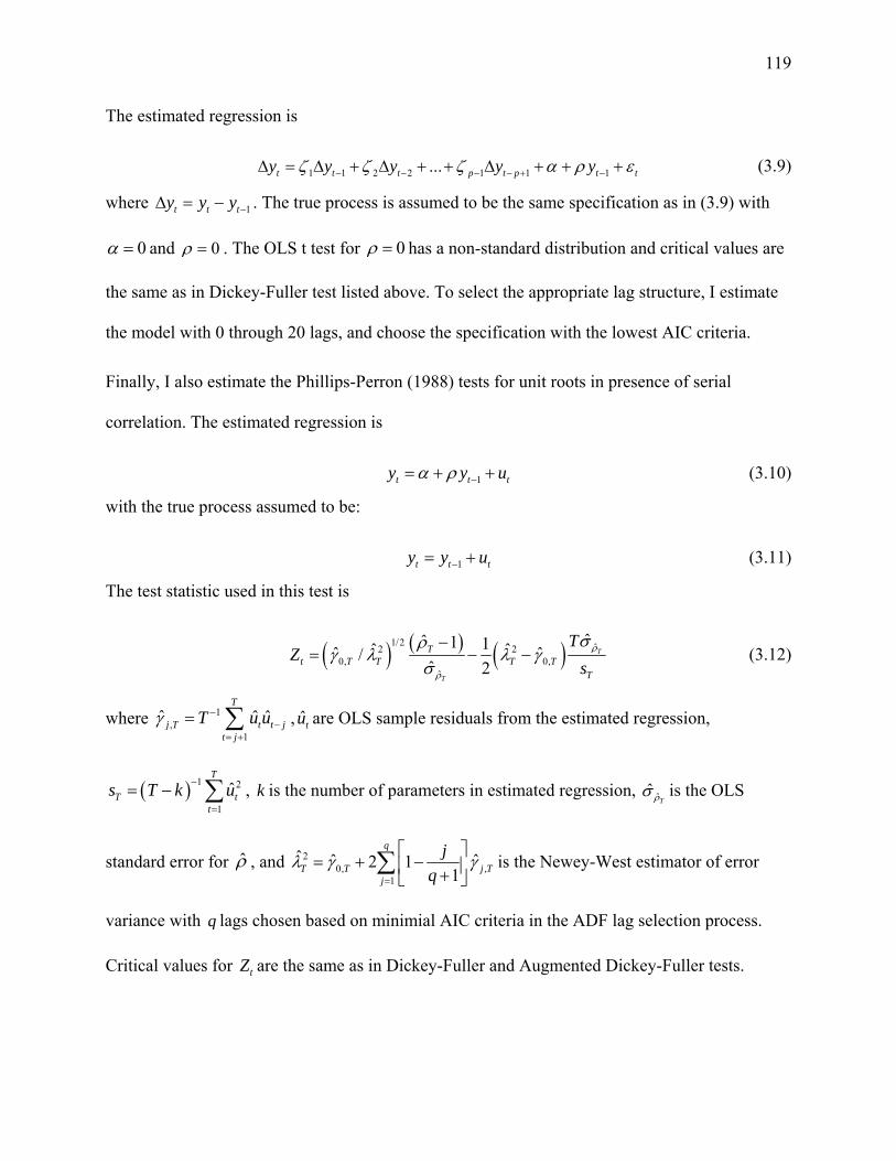
119
The estimated regression is
1 1 2 2 1 1 1...t t t p t p t ty y y y y (3.9)
where 1t t ty y y . The true process is assumed to be the same specification as in (3.9) with
0 and 0 . The OLS t test for 0 has a non-standard distribution and critical values are
the same as in Dickey-Fuller test listed above. To select the appropriate lag structure, I estimate
the model with 0 through 20 lags, and choose the specification with the lowest AIC criteria.
Finally, I also estimate the Phillips-Perron (1988) tests for unit roots in presence of serial
correlation. The estimated regression is
1t t ty y u (3.10)
with the true process assumed to be:
1t t ty y u (3.11)
The test statistic used in this test is
1/2 ˆ2 20, 0,
ˆ
ˆˆ 1 1ˆ ˆˆ ˆ/ˆ 2
T
T
Tt T T T T
T
TZ
s
(3.12)
where 1,
1
ˆ ˆ ˆT
j T t t jt j
T u u
, ˆtu are OLS sample residuals from the estimated regression,
1 2
1
ˆT
T tt
s T k u
, k is the number of parameters in estimated regression, ˆˆT
is the OLS
standard error for ̂ , and 20, ,
1
ˆ ˆ ˆ2 11
q
T T j Tj
j
q
is the Newey-West estimator of error
variance with q lags chosen based on minimial AIC criteria in the ADF lag selection process.
Critical values for tZ are the same as in Dickey-Fuller and Augmented Dickey-Fuller tests.
120
RATS 8.01 was used for these tests as it provides the user with easy-to-use commands for the
tests as well as selecting the optimal lag structure to be used in the ADF and Phillips-Perron
tests.
It has been noted that results of unit-root test may vary with data frequency (Tomek and Wang,
2007), so I estimate these tests for both daily and weekly data frequency. In addition, since CME
cash market for cheese is not very liquid, and sales transactions do not occur on about 40 percent
of trading days in the sample, I construct an irregular frequency data keeping only those days
when the cash market did in fact record a sales transaction either in 40lbs cheese blocks or
500lbs cheese barrels.
Perhaps due to low cash market liquidity, it is a custom in the cheese industry to report the last
uncovered offer or last unfilled bid as the closing cash price for the day. While our primary cash
price series only contains sales records, it may be of interest to examine if any of the results
regarding cash/futures information flow are sensitive to the choice of cash price series (i.e.
closing sales price vs. closing prices that may be a bid or offer). For that reason, I perform unit
root tests on these publicly reported closing cash prices as well, and denote them with a (B/O)
suffix to differentiate from the regular sales price series. In addition, I account for potential
seasonality in cash prices by testing for the presence of unit roots in the residuals from
regressions of cash prices on quarterly indicator variables rather than testing for unit roots in
cash prices directly.
I examine the sensitivity of ADF test results to the specification of lagged prices in the estimated
regression. Recall that the futures price series is always an n-th nearby series, i.e. concatenation
of segments taken from different futures contract months at the time when those contracts were

121
the n-th contract to maturity. Denote by itf a futures price on time t for a contract expiring at iT .
Then jth-nearby is a sequence of futures prices that can be represented as
1 1 1 1 1 1 1
1 1 1 21 1 2 1... , ,..., , , ,..., , ...
i j i j i j i j i j
i i i i i i ij t t T T T T TF f f f f f f f
(3.13)
For example, the 2nd nearby futures price series is constructed by taking the prices of the
February contract in the month of January, the March contract in the month of February, etc.
Notice that in such a nearby series from time to time two consecutive prices will correspond to
different contract months. For example, when the January contract settles, the 2nd nearby futures
price will be the one from March, while one day earlier, i.e. on the last day the January contract
traded, the 2nd nearby futures price will refer to a February contract futures price. As a
consequence, using inbuilt software commands that do not account for this information will
produce differenced prices for equation (3.9) that are occasionally corresponding to different
contract months. To check if this is influencing the test results, I estimate a regression that
insures that differenced prices always come from the same contract month, but is other otherwise
equivalent to regression estimated by the inbuilt RATS command, i.e. the number of lags are
determined via AIC criteria. In particular, I estimate the following regression
1 1 2 2 1 1 1...t t t p t p t tf f f f f (3.14)
where 1i i
t t tf f f and right hand side variable 1 1i
t tf f .
Finally, to account for possible sensitivity to the choice of rollover date, I perform unit root tests
of nearby series that are constructed by rolling over included contracts on the days when the 1st
nearby contract expires, as well as on the day when the 1st nearby has 3 trading days to maturity
left.
122
Results of the unit root tests are presented in Table 3.1. The null hypothesis of unit roots is
strongly rejected for cash cheese prices. This holds true irrespective of the data frequency used,
whether 40lbs blocks or barrels are examined, and whether the series is based on sales prices or
publicly reported daily closing prices that may include unfilled bids and uncovered offers.
The situation is more complex in unit root test results for nearby futures prices. The ADF test
for unit roots rejects the null for the second nearby futures series at a 5% confidence level
irrespective of the data frequency used, while data frequency seems to matter for the 3rd, 4th and
5th nearby series. Irrespective of the rollover procedure used, tests done with weekly data are
more likely to reject a unit root. The Phillips-Perron statistics are generally higher for weekly
data frequency than those obtained using daily and sales only frequency. For daily and sales-only
data, with the exception of the 1st nearby contract, the ADF test statistic falls as time-to-maturity
increases, i.e. the ADF t-statistic is higher for the 2nd nearby than for the 3rd nearby, etc. The
most striking result is the difference in t-statistics from the regular ADF regression that does not
account for contract rollovers in constructing differenced prices, and the equivalent regressions
that do. When regressions like (3.14) are estimated, the t-statistics next to lagged price of the
same contract are very small, and the null hypothesis of unit roots is never rejected. This happens
regardless of data frequency, time to maturity horizon and rollover method used. Regressions
(3.14) evaluate the time series properties of within-contract segments, ignoring dynamics at
contract rollovers. Therefore, these results suggest that unit root results based on ADF
regressions may be driven by the nature of the price changes at the rollover time. In particular,
this indicates that nearby futures price series are nonlinear - martingales within each contract
segment, and mean-reverting at contract rollovers. As rollovers occur more frequently for weekly
123
data the explanation offered above is consistent with unit roots tests more strongly rejecting the
null for weekly data series.
Of special interest is evaluating the time series properties of the cash-futures price spread,
denoted ,n td and defined as the difference between contemporaneous average cash prices and n-th
nearby futures price , ,n t t n td c f . In this context the cash price is a simple average of blocks
and barrels cash sales prices for a particular day. Results are reported for spreads calculated
using second and fifth nearby futures, and spreads are always found to be strongly stationary. If
the fifth nearby futures were indeed nonstationary, and if the cash price was truly stationary, then
no linear combination of the two series could be stationary. The fact that the null is strongly
rejected for spreads using the fifth nearby futures is additional evidence suggesting there are
nonlinearities in the nearby futures prices.
There are three questions that naturally arise as a reaction to these results. First, what does
economic theory suggests about the time series properties of cash and futures commodity prices?
Second, what kind of nonlinearities should we expect in nearby futures prices, when cash prices
are stationary? And finally, what is the appropriate way to model information flows between
cash and futures markets in the face of observed stationarity in cash prices and nonlinearities in
nearby futures prices. The first two questions are answered in the next subsection, while the
model specification issues are left for the next part of the paper.
3.4.2. Economic Theory and Time Series Properties of Agricultural Cash and Futures
Prices
Early studies of cash/futures linkages used regression in price levels or differenced series (e.g.
Oellerman and Farris, 1985). However, in many commodities, and especially when using daily
124
data, researchers have found that both cash and futures contain unit root (e.g. Schneider and
Goodwin, 1991; Ivanov and Cho, 2011). These findings have been disputed both on theoretical
and statistical grounds. As far as theory is concerned, it has been claimed that agricultural price
theory does not support the hypothesis that all shocks to prices are persistent (Tomek and Wang,
2007). Furthermore, misspecified models that do not account for structural breaks may bias the
results towards accepting the null hypothesis of unit root presence, and unit roots test that have
low power will not be effective in differentiating between integrated and stationary, but highly
persistent time series (Geweke and Porter-Hudok, 1983).
Theoretical priors regarding time series properties of cash and futures prices are remarkably
different. As far as cash price is concerned, the fundamental property of prices emerging in
perfectly competitive markets is the necessity of zero long-run economic profit for the marginal
producer. That condition implies that profit margind will be a mean-reverting time series.
Consequently, if the long-run industry average cost curve is flat (a case of constant returns to
scale), any permanent shift in the demand function will produce only temporary shock to cash
prices, while permanent changes in input costs will shift the long-run average cost curve and thus
induce a structural change in cash price series. Even with constant long run average costs, if
production cannot adjust quickly to demand shocks in the short run, cash prices may exhibit high
a degree of persistency and rather slow reversion to long-run averages. Finally, if returns to scale
are either decreasing or increasing, shifts in demand will manifest as permanent shocks to cash
price series.
While the time series properties of cash prices are argued based on production theory, the time
series characteristics of futures price series emerge from finance theory. If the futures market is

125
efficient (i.e. if futures prices fully account for all available information) then prices within a
single contract will be martingales if the marginal risk premium is zero, submartingales if
marginal risk premium is positive (i.e. futures are downward biased and traders having long
position are rewarded), and supermartingales if the marginal risk premium is negative (i.e.
futures are upward biased and traders having short position are rewarded). In each case, by
deducting the marginal risk premium we can arrive at a martingale series whose direction of
change cannot be predicted based on concurrently available information. From this it follows that
whether the risk premium is present or not, efficient futures prices will be nonstationary, i.e. all
shocks to futures prices are permanent.
Suppose now that there exists a second-order stationary cash price series for some commodity,
and that a futures contract is written on that commodity. Assume further that there is no basis at
futures contract expiry, i.e. the terminal futures price equals the cash price prevailing at contract
expiry. Finally, assume that futures prices are efficient and embody no risk premium. What will
be the time series properties of an n-th nearby futures price series?
Let be the unconditional mean of the cash price, and 2c be the unconditional variance. By the
Wold decomposition theorem (Wold, 1954) we know that there exists the unique fundamental
moving average representation of the cash price stochastic process:
0
t i t ii
c
(3.15)
where 0 1. Denote futures price at time t for a contract that expires at time T by Ttf . Efficient
futures prices that do not incorporate risk premiums will be unbiased predictors of cash prices at
contract expiry:
Tt t Tf E c (3.16)
126
Using Wiener-Kolmogorov prediction formula (Hansen and Sargent, 1980) we can express
futures prices at time t as
0
Tt t T t i t iT t
i
Lf
L
(3.17)
where the annihilation operator replaces all negative lag values by zero. An alternative, and
equivalent expression for (3.17) is
Tt i T i
i T t
f
(3.18)
We first exploit notation in (3.18) to show that under the assumptions of this model, any change
to futures prices of a single contract must come from unanticipated information shocks 1t .
First, express 1T
tf using Wiener-Kolmogorov formula as
1 1 1 11( 1)
T Tt i T i i T i t t T t tT t
i T t i T t
f f
(3.19)
Since 1 0t tE it follows that 1T T
t t tE f f and we have established the martingale property
of futures prices of the same contract. If in addition fundamental moving average coefficients
increase in absolute value as their index decreases (this would be the case for AR(1) models for
example) then the conditional variance of futures prices
2 21 1
Tt t T t cVar f (3.20)
will be increasing as time to maturity decreases. This is the well-known “Samuelson Effect“.
From the analysis undetaken above, it would be wrong to conclude that because prices within a
single futures contract are martingales that such must also be true for an n-th nearby futures price
series. Let the first nearby futures price series be constructed by rolling contracts over one day
before the delivery date:
127
31 1 2 2
1 1 2 21 1 1 1,..., , ,... , ,...TT T T TT T T TF f f f f f (3.21)
Let us take a closer look at the MA representation of futures prices around the rollover date:
1
1 1
1
1 11
k
k k k k
k
k k k k
k k
TT T T i T i
i
TT T T i T i
i T T
f E c
f E c
(3.22)
The difference in consecutive futures prices of this nearby series at rollover time is
1
1 111
k k
k k k k k k k k
T TT T T T T T T i i T i
i
f f
(3.23)
Only the first part of the difference, 1k k kT T T , is not known at time 1kT , while the second part,
the infinite sum, is fully known at that time. It follows that
1
11 1 11
k k k
k k k k k k k
T T TT T T T T i i T i T
i
E f f f
(3.24)
The first nearby futures price series will not have the martingale properties, and changes in the
nearby price sequence at rollover time are partially predictable. To give a simple example,
suppose that current first nearby contract is the March contract, and tomorrow the first nearby
contract will be the futures price for delivery in April, i.e. rollover is to occur tomorrow. Then
the expected change in the first nearby price series is the simple difference between today's price
for April delivery and today's price for March delivery.
We can extract some further insight from (3.24). If it so happens that the cash price at time
1kT , 1
1k kT i T i
i
c
is above the long run mean , then the sum 1
ki T ii
will be
positive. When fundamental moving average coefficients are monotonically declining in absolute
value, i.e. , , 0i ji j a i j then the infinite sums from expression (3.22) can be
ordered in absolute value:
128
1
1 1k k
k k
i T i i T ii T T i
(3.25)
If condition (3.25) holds, and 1kTc then
11
0k k kT T i i T i
i
. In other words, the
predictable component in the first nearby price change at contract rollover will be mean-
reverting. In addition, because cash price is assumed to be second-order stationary, moving
average coefficients are square summable, i.e. 2
0i
i
. This implies that
lim 0i i (3.26)
Since for a fixed t kk T t it follows that
1 1
0
lim lim lim
lim lim
k
k k k k
k k
Tk t T k t T T k t T
k t j T j k T t j t jj i o
E f E E c E c
E
(3.27)
In words, the long-run expected value of the first nearby futures price series is the unconditional
mean of the cash price. This characteristic is shared with any second-order stationary series: if a
variable is second-order stationary then forecasts of the variables value far into the future will
eventually converge to an uninformed prior which is the unconditional mean of the variable.
That must be so since any shocks that explain current deviations of that variable from its
unconditional mean will eventually die out. The result that the long-run forecast of the first
nearby futures price series is the unconditional mean of the cash price stands in sharp contrast to
characteristics of series that exhibit martingale properties. For such a series, limk t k tx x ,
i.e. all shocks are permanent, and the long-run forecast is equal to the last observed value of the
variable.

129
The argument that the first nearby price series will be mean-reverting at contract rollover carries
forward to the n-th nearby series. Let us compare the first and an n-th nearby price series at
rollover. For the first nearby series, price change at rollover time is given in (3.23). Since futures
prices are assumed unbiased predictors of future cash prices, we can rewrite (3.23) as
1
11 1k k
k k k k k k
T TT T T T T Tf f E c E c
(3.28)
Similarly, for the n-th nearby price series, 1
11 1k n k n
k k k k n k k n
T TT T T T T Tf f E c E c
. From (3.26) it
follows that
11lim 0k n k n
k k
T Tn T Tf f (3.29)
In other words, the predictabile part of price change for n-th nearby contract at rollover time will
be smaller the higher the n is. Mean-reverting changes at contract rollover will be most
pronounced in the first nearby, less so in the second nearby, and even less in the third nearby
price series, etc.
In conclusion, I have illustrated using a simple example that when the cash price series is
second-order stationary, futures prices for a specific contract will be a martingale, but not a
random walk, as random walk assumes constant variance of shocks, and in we expect to see the
Samuelson effect, i.e. increases in futures price volatility as time to maturity declines.
Furthermore, the n-th nearby futures series will be nonlinear, having martingale properties within
each contract segment, and mean-reverting changes at contract rollover. When fundamental MA
coefficients are monotonically declining in absolute value, mean-reverting change at contract
rollover will be less prononuced for further horizon series.
130
Suppose that we apply unit root tests that assume linearity in the variable being tested and posit
as a null hypothesis that the process contains a unit root, e.g. a Dickey-Fuller type test or
Phillips-Perron test. Based on these insights we would expect to see the following:
1) The null hypothesis will likely be rejected for cash prices
2) The null hypothesis will likely not be rejected for a single contract futures price series
3) The null hypothesis will be more likely to be rejected for n -th nearby than for 1n -th
nearby.
4) The more observations there are between rollover periods, the less likely the null
hypothesis will be rejected. Consequently, reducing data frequency increases the
likelihood of rejecting the null hypothesis.
The results we obtained for unit root tests applied to cheese cash and nearby futures prices are
consistent with these predictions. In particular,
1. The null is always rejected for cash prices
2. Regressions like (3.14) that test for unit root presence in contract segments, and ignore
dynamics at contract rollovers never reject the null hypothesis.
3. For daily and sales-only data frequencies, test statistics for ADF and Phillips-Perron tests
mostly decline from 2nd to 5th nearby series, although I not test if they are statistically
significantly different.
4. Unit roots are rejected for all tested nearby series when weekly frequency is used, but
tests fails to reject unit roots for a majority of the nearby series when higher data
frequency is employed.

131
We should also notice that not all predictions of the model above hold for cash markets. In
particular, for daily and sales-only data the test statistic used in the ADF test is higher for second
than for the first nearby series, indicating a stronger mean-reversion at rollover time for the
second series. This should not be surprising, however, as I have shown in another part of the
thesis that volatility of futures prices declines dramatically in the last 4 weeks of contract life.
This may be due to formula-based contract settlement procedure. In conclusion, my simple
forecasting model demonstrates a high ability to explain observed patterns in unit-root tests
results.
3.5. Information flows between cheese cash and futures markets
When examining the information flow between cash and futures markets, it is standard practice
to use the cointegration framework developed by Johansen and Juselius (1990). Bessler and
Covey (1991) were among the first to introduce this method to commodity price analysis.
Examples relevant for this chapter include Fortenbery and Zapata (1997) and Thraen (1999),
papers that applied co-integration to analyses of dairy futures and cash markets. In this section, I
first define the concepts of causality as they are commonly understood and used in modern
applied econometrics. Next I discuss causality in mean, better known as ‘Granger causality’,
causality in variance and second-order causality as well as testable restrictions on model
parameters that correspond to these concepts. I then propose an error-correction model
incorporating GARCH structure on errors as a framework to examine information flows between
cheese cash and futures markets. Given the apparent stationarity of cheese cash prices, coupled
with nonlinearities in nearby futures prices, I build a model similar to an error-correction model,
with the role of cointegrating vector taken by the spread between cash and the 2nd nearby futures
price. The addition of a GARCH error structure allows us to examine volatility spillovers
132
between the cash and the futures markets. In addition, the GARCH structure results in a
framework that allows us to perform a preliminary examination of the role of speculators on
market volatility when available data on trader positions has low frequency.
3.5.1. Concepts of Causality
Operational definitions of causality are summarized in Granger (1980). Consider a universe in
which all variables are measured at prespecified time points at constant intervals 1, 2,...t We
are interested in the possibility that a series ty causes another series tx . Let nI be an information
set available at time n , consisting of terms of the series tx
: , 0n n jI x j (3.30)
Denote an information set that includes information on both series tx and ty with nJ
: , 0n n j n jJ x y j (3.31)
Let 1 |n nF x I be the conditional distribution of 1tx given nI with conditional mean
1 |n nE x I .
Non-causality in distribution occurs if ny does not cause 1nx with respect to nJ , or
1 1| |n n n nF x I F x J (3.32)
In other words, knowing the history of variable y does not improve probabilistic forecasts of the
variable x . For the sake of completeness, we should state that Granger defined non-causality and
causality differently. Let n be the universal information set, i.e. a set containing all the
information in universe available at time n . Then ny is said to cause 1nx if
1 1| |n n n n nF x F x y (3.33)

133
The difference between the concepts of non-causality and causality is large, if we adhere strictly
to definitions (3.32) and (3.33). The former equation requires us to observe only histories of the
series tx and ty while the latter expression stipulates omniscience. Given the definitions above,
rejecting non-causality is necessary, but not sufficient to demonstrate causality. In defining the
non-causality in mean and variance, we follow the exposition by Comte and Lieberman (2000).
Non-causality in mean occurs if ny does not Granger cause 1nx in mean, denoted as 1
G
n ny x ,
or
1 1| |n n n nE x I E x J (3.34)
Given some information set n , the conditional variance of the one-step ahead forecast will be
2
1 1 |t t n nE x E x
. Non-causality in variance was first introduced in Granger, Robins
and Engle (1986). We follow Comte and Lieberman (2000) in differentiating between non-
causality in variance and second-order non-causality.
Non-causality in variance happens when variable ny does not cause 1nx in variance, denoted
1
V
n ny x , or
2 2
1 1 1 1| |n n n n n n n nE x E x I I E x E x J J (3.35)
Second-order non-causality, denoted 1
GRE
n ny x , is obtained if
2 2
1 1 1 1| |n n n n n n n nE x E x J I E x E x J J (3.36)
Unlike non-causality in variance which fully restricts the information set used in forecasting, in
second-order non-causality information from ny is allowed to be utilized in calculating the
134
conditional mean of 1tx , but not the expected square deviation from the conditional mean. In
this terminology, the concept of causality in second moments, as introduced by Granger, Robins
and Engle (1986), corresponds to second-order non-causality. The relationship between non-
causality in mean, non-causality in variance and second-order non-causality is as follows:
1 1 1 and V G GRE
n n n n n ny x y x y x
(3.37)
It suffices to show that ny Granger causes 1nx in the mean to establish variance causality. This
renders second-order non-causality a more interesting concept, for it is neither necessary nor
sufficient for causality in means to exist for second-order causality to be present.
3.5.2. Testing for Second-Order Non-Causality
Cheung and Ng (1996) propose a two-step approach where the first step consists of estimating
univariate time series models that allow for a time-varying conditional mean and variance, i.e. a
univariate GARCH(1,1) model. In the second stage, residuals of the univariate models are
squared and standardized by dividing with the conditional variance. The square-standardized
residuals are then utilized in a cross-correlation function (CCF) to test for the presence of
causality in variance. The authors argue that this method may be superior to multivariate
GARCH modeling because it is simpler to implement, and does not rely on correctly specifying
the functional form of inter-series dynamics.
Comte and Lieberman (2000) show that in GARCH models with a BEKK conditional covariance
structure, second-order non-causality is equivalent to specific restrictions on ARCH and GARCH
parameters. Consider a BEKK representation of a bivariate GARCH(1,1) model as suggested by
Engle and Kroner (1995). The conditional covariance, tH is given by the formula
135
0 0 1 1 1t t t tH C C A A G H G (3.38)
with
1,11 21 11 12 11 12
21 22 21 22 21 22 2,
t
t tt
h h a a g gH A G
h h a a g g
In the covariance matrix tH , 11h is the conditional variance of the first series, 22h is the
conditional variance of the second series and 12 21h h is the conditional covariance between the
series. Given that expressions for ARCH and GARCH in the conditional covariance are written
in (3.38) as a quadratic form, it will help our intuition to rewrite it in a simpler way.
2 2 2 2 2 2 2 211 1 11 1, 1 11 21 1, 1 2, 1 21 2, 1 11 11, 1 11 21 12, 1 21 22, 1
2 212 2 11 12 1, 1 21 12 11 22 1, 1 2, 1 21 22 2, 1
11 12 11, 1 21 12 11 22 12, 1 21 22 22, 1
2 2t t t t t t t
t t t t
t t t
h c a a a a g h g g h g h
h c a a a a a a a a
g g h g g g g h g g h
2 2 2 2 2 2 2 2
22 3 22 1, 1 22 12 1, 1 2, 1 12 2, 1 22 22, 1 22 12 12, 1 12 22, 12 2t t t t t t th c a a a a g h g g h g h
(3.39)
Let tx be indexed as the first and ty as the second series in the model above. Comte and
Lieberman show that the second-order non-causality and coefficients of the BEKK GARCH(1,1)
correspond as given below.
1 21 210, 0GRE
n ny x a g (3.40)
One reason Cheung and Ng opted to pursue a cross-correlation function approach was that at the
time, asymptotic theory was not worked out for multivariate GARCH. In fact, Comte and
Lieberman warn us in 2000 that while it was a common practice to employ likelihood-based
tests, such as Wald, Lagrange multiplier test or likelihood ratio test to evaluate statistical
properties of restrictions on GARCH parameters, the asymptotic distributions of these tests in the
general multivariate GARCH(p,q) were still unknown. Fortunately, Comte and Lieberman
(2003) and Ling and McAleer (2003) prove both consistency and asymptotic normality of quasi-
maximum likelihood estimator. That enables us to use the standard approach in testing second-
136
order non-causality. In particular, to test the restrictions of (3.40) we need to estimate both
restricted and unrestricted model. Under the null hypothesis of second-order non-causality,
critical value of the test statistic will be given by 2 2,0.95 5.9915
3.5.3. Model for Evaluating Information Flows Between Cash and Futures Cheese Prices.
In previous section the time-series properties of cash and nearby futures price were evaluated.
Given the results, it makes little sense to pursue a standard cointegration approach, for cash price
is clearly not an integrated process, and nearby futures price seems to be a nonlinear
concatenation of unit-roots within-contract segments and mean-reverting changes at contract
rollovers. The basic idea of cointegration is that if two integrated variables get too far apart, at
least one of them will adjust to bring the variables closer together. A framework that allows the
difference between cash and futures cheese price to carry valuable forecasting information seems
like a rather reasonable approach. We have seen that such spreads exhibits strong mean-reverting
characteristics, so the model that naturally presents itself is the following:
1 11 1 1 11 1 1 1 1 1
2 21 1 2 21 1 2 2 1 2
... ...
... ...
i it t p t p t p t p t t
i i it t p t p t p t p t t
c c c f f d
f c c f f d
(3.41)
where 1 1 1i
t t td c f , and all futures prices are for the second nearby contract, with i being the
contract month/year index of the second-nearby contract at time t . In the above model,
information flow between the two markets can arise from two effects. First, short-term dynamics
may be important. For example, if the futures market closes the day higher than yesterday, that
may help predict the direction of cash cheese prices the following morning. The predictive power
in this example may originate from several different causal mechanisms. First, it may be that
futures prices have discovered new information, and the cash price will incorporate it in the next
137
trading session. Alternatively, it may be that traders in both markets get the information at the
same time, but if futures market is open for trading, and cash market already closed for the day
then the first lag of the changes in futures prices could have predictive power simply due to
differences in market trading hours. This could happen even if no additional price discovery in
futures markets took place. The other source of information flow may come from the spread
between the cash and the second nearby futures price. Second nearby contracts have time to
maturity between 22 and 44 trading days. The cheese futures contract is financially settled
against the USDA announced national average monthly cheese price that will closely match the
average of CME cash prices observed from 30 to 10 trading days to maturity. If the spread
between the cash and futures price is large, one of these two variables will have to eventually
adjust and reduce the spread. If futures prices accurately anticipate the average cash price near
the contract expiry, then the spread between cash and the futures price will have forecasting
power in predicting changes in cash prices.
Given the definition of Granger non-causality in mean, we can state that futures prices do not
Granger cause cash prices if the following restrictions on model coefficients hold:
1
1
0, 1,..,
0i i p
(3.42)
For non-causality from cash to futures prices the same restrictions are to be applied to the
corresponding coefficients in the second equation of the model (3.41).
In addition to forecasting price changes, we are interested in volatility dynamics and spillovers
between the two markets. One approach would be to add the BEKK structure to errors as in
(3.38). In addition to spillovers, we are interested in evaluating the impact of speculative activity

138
on volatility levels and dynamics. A standard method to include additional regressors to BEKK
variance model is to expand the structure to what is called BEKK-X:
10 0 1 1 1 1
2
~ 0, 'tt t t t t t
t
N H H C C A A G H G D Dx
(3.43)
Given that the coefficients next to the additional regressor enter variance equation (3.43) as a
quadratic form, the sign of the coefficients for the impact on variance of both cash and futures
prices is always restricted to be positive. To see that, expand 1' tD DS as follows
2 2
11 11 11 211 1 12
21 22 21 22 21 22 22
0 0' t t t
d d d dD Dx x x
d d d d d d d
(3.44)
It turns out that the BEKK specification can only test if the increase in an additional regressor in
the variance equation is associated with an increase in the conditional variance of cash and
futures prices. As such, a hypothesis that speculation may reduce the conditional variance of
futures price cannot be easily tested with this model specification, and an alternative model
structure needs to be developed.
One possibility would be a bivariate EGARCH model introduced first by Koutmos and Tucker
(1996) to evaluate dynamic interactions between spot and futures in the stock markets. Following
Nelson (1991), it is the logarithm of the conditional variance in their EGARCH model that is
modeled as a linear function of past conditional log-variances and magnitude of realized shocks
in the previous period. Exponential form allows this modeling approach to admit additional
regressors in the variance equation while preserving the positive definiteness of the conditional
covariance matrix. Similar models were used by Tse (1999), Bhar (2001), Zhong, Darrat and
Ottero (2005) and Bhar and Nikolova (2009).
139
While variations of the bivariate EGARCH model used by these authors allows for high degree
of flexibility, the exponential form may present estimation problems. In addition, it may be of
help to have a model that nests a BEKK model with means as in (3.41) and variance model as in
(3.38) as a special case where additional regressors in the variance equation are found to have no
influence on the variance dynamics.
In what follows, we expand the BEKK model without imposing a particular sign on the
coefficient of the additional regressor in the variance equation, while preserving the positive-
definiteness of the conditional covariance matrix. Let the mean model be as in (3.41).
We introduce additional regressors in the variance equation through an exponential function that
multiplies the BEKK structure. In a standard BEKK model, we have
10 0 1 1 1
2
~ 0, tt t t t t
t
N H H C C A A G H G
(3.45)
We can expand the variance model in the following way
1
2
~ 0, tt t t t
t
N H H X H
(3.46)
where tH is given by the expression in (3.45), the symbol stands for Hadamard product, i.e.
element-by-element multiplication, and the matrix tX is defined as
1 1
12 1 2 1
t
t t
x
t x x
eX
e e
(3.47)
Due to the BEKK form, tH will be positive definite, and to insure positive definiteness of tH it
will suffice to impose the following restriction on the parameter 12 :
12 1 2
1
2 (3.48)
140
As I shall demonstrate, restriction (3.48) is equivalent to restricting the impact of additional
regressors to have influence only on conditional variances of the two series, but not on their
conditional correlation. Denote the elements of tH as
11,
12, 22,
tt
t t
H
(3.49)
Since the exponential form is used for all elements of tX , the diagonal elements of tH will be
positive. To insure positive definiteness of tH and it will be sufficient that the determinant of the
tH matrix is positive.
1 1 2 1 12 12
11, 22, 22, 0t t tx x xt t t tH e e e (3.50)
With restriction (3.48) this is reduced to
1 1 2 12
11, 22, 22,t tx x
t t t tH e (3.51)
The positive range of the exponential function together with positive-definiteness of tH imposed
by the BEKK structure jointly guarantees that tH will be positive-definite. In practice, I
recommend starting with the unrestricted version given in (3.47), and after the model is
estimated checking for positive-definiteness of the conditional covariance matrix for each
observation. If that is violated for any data point, the stated restriction will resolve the problem.
I propose that this new GARCH model be called GARCH-MEX, or BEKK-MEX, where MEX
stands for multiplicative exponential heteroskedasticity induced by additional regressors.
GARCH-MEX may be estimated in two variations, depending on whether a researcher believes
that the impact of an additional regressor is exhausted in the present period or propagated
forward through the GARCH structure. In the first case, we would model the variance with
141
1
2
0 0 1 1 1
~ 0, tt
t
t t t
t t t t
N H
H X H
H C C A A G H G
(3.52)
and in the second case, the BEKK structure for tH would be modified to
0 0 1 1 1t t t tH C C A A G H G (3.53)
In words, specification (3.53) allows the impact of additional regressors to influence future
variances through the GARCH structure.
GARCH-MEX has four important characteristics:
1) If additional regressors do not explain volatility, i.e. 1 12 2 0 , the model collapses
to a standard BEKK model.
2) Since the exponential function is always positive, signs of coefficients 1 2, do not need
to be restricted as in (3.44).
3) The covariance matrix is always positive definite, as demonstrated in (3.51).
4) With restriction (3.48) additional regressors impact only conditional variances of
individual series, but not conditional correlation directly.
1 2 1
1 1 2 1
1
212, 12, 12,
1 111, 12, 11, 22,2 2
11, 22,
t
t t
S
t t t
S St t t t
t t
e
e e
(3.54)
However, conditional correlation is time-varying, and in specification (3.53) influenced by
additional regressors indirectly, through impacts on lagged conditional variances that enter the
BEKK structure.
142
The complete model for evaluating information flows between cash and futures prices, and the
influence of speculators on volatility dynamics is as follows:
1 11 1 14 4 11 1 14 4 1 1 1
2 21 1 24 4 21 1 24 4 2 1 2
... ...
... ...
i it t t t t t t
i i it t t t t t t
c c c f f d
f c c f f d
(3.55)
1
2
0 0 1 1 1
~ 0, tt
t
t t t
t t t t
N H
H X H
H C C A A G H G
(3.56)
1 1 1 1
12 1 12 1 2 1 2 1
t t
t t t t
S c
t S c S c
eX
e e
(3.57)
In the MEX matrix, I have used lagged cash prices in addition to a measure of speculative
adequacy, to control for possible confounding if speculative activity coincides with cycles in
milk prices.
The model can be estimated in several variations. First, prices can be expressed as either levels
or logarithms. Second, data frequency can be daily, ‘sales-only’ or weekly. However, for daily
and ‘sales-only’ frequencies we cannot estimate the impact of speculators as that data is only
available on a weekly basis. I test 14 different measures of speculative adequacy which are
described in the next section. We may test both variations of GARCH-MEX model, i.e. allowing
additional regressors to have an effect that propagates dynamically through the GARCH
structure as in (3.56) or restrict the BEKK structure to
0 0 1 1 1t t t tH C C A A G H G (3.58)
Finally, we may impose the restriction
12 1 2
12 1 2
1
21
2
(3.59)
143
to test if conditional correlation is impacted by speculative activity and cash price levels.
3.5.4. Measures of Speculative Adequacy
To evaluate the impact of speculators on cheese markets, we use a measure of speculative
activity in Class III milk futures prices. We chose Class III milk futures as it is the most liquid
dairy futures market, and tied to cheese futures through a no-arbitrage condition that connects
futures prices for butter, cheese, whey and Class III contracts. In the absence of trading costs,
cheese futures price can be represented as simple linear combinations of butter, whey and Class
III milk prices. Thus, whichever variable influences the conditional variance of Class III milk
futures, it will influence the conditional variance of cheese futures price as well. Data for
speculators’ position are obtained from Commitments of Traders (COT) report published weekly
by the Commodity Futures Trading Commission (CFTC). COT only presents data for selected
markets that the CFTC considers to be important to monitor closely, and cheese futures are not
currently included in the COT report.
A classical measure of speculative adequacy is called Working’s T, and was introduced by
Working (1960, May). Denote commercial (hedging) long positions with LH , SH is the
commercial short position, LS is the noncommercial (speculative) long, and SS speculative short
positions, all measured by the amount of contracts held. When short hedging exceeds long
hedging, Working’s T is calculated as
2
1 SL L
S L S L
SS HT
H H H H
(3.60)
If the hedging position is net long, i.e. L SH H then the formula becomes
1 L
S L
ST
H H
(3.61)
144
To calculate T, all open interest (excluding noncommercial spreading) has to be allocated to
these four categories ( LH , SH , SS , LS ) . That means that nonreportable positions, for which we
have no information relative to their speculative or hedging nature, have to be allocated to the
above categories. Working’s T measures the ‘adequacy’ of speculation. The minimum value is
equal to 1. Markets with T-index less than 1.15 are considered to have insufficient liquidity
(Irwin and Sanders, 2010).
There are at least nine ways to allocate nonreportable positions in the calculation of Working’s
T-index. First, we may allocate them in such way as to obtain the upper or lower bounds of the
index as in Peck (1980). We denote these calculations as “upper bound” and “lower bound”.
Another approach would be to base the allocation rules on informal feedback based on personal
conversations from brokers managing accounts of traders in class III milk. It was suggested to
me by Mr. Phil Plourd, the manager of a company that was among the first to offer risk
management services to dairy sector, that it might be reasonable to treat all nonreportable short
positions as commercial, and split nonreportable long positions equally between the speculative
and hedging categories. Working’s T calculated in such way is reffered to as “industry”. Irwin
and Sanders (2010) follow Rutledge (1977) and allocate nonreportable positions to the
commercial, noncommercial and index trader categories in the same proportion as that which is
observed for reporting traders. Denote index obtained using their method as “proportional”.
The problem with this approach is that it ignores the similarity between position profiles of
nonreportables and the stated three categories. To illustrate this point with a simple example we
shall ignore the role of index traders for a moment and assume all reportable positions are
classified to the noncommercial and commercial categories only. If commercials represent the
predominant percentage of open interest, the above approach would classify most nonreportables
145
as commercials. However, it may be the case that commercial traders have a very strong net-long
positions, while both non-commercials and nonreportables have strong net-short position. In that
sense, nonreportables seem to have a position profile that is more like non-commercials than like
commercials.
For example, consider the situation in Class III milk futures market on September 12, 2000.
Ignoring noncommercial spreading positions, the relative noncommercial short position
measured as / ( )S S SS H S was only 13.24%, and the relative noncommercial long position,
measured as / ( )L L LS S H was even lower, only 5.90%. According to the Irwin and Sanders
approach, only 13.24% of nonreportable shorts and 5.90% of nonreportable long positions would
be allocated to noncommercials short and long positions respectively. Now consider the
percentage net-long positions for all trader groups. Define relative net-long position for a
particular group as
% 100L S
NLL S Spr
(3.62)
where L stands for long, S for short, and Spr for spreading.
On 9/12/2000, the percentage net-long position was -29.68% for noncommercials, 13.7% for
commercials and -29.77% for nonreportable positions. According to this metric, nonreportables
were very similar in their position profile to noncommercials, and it may make sense to allocate
more than just a marginal fraction of those contracts to the noncommercial group.
Consider a following allocation rule. Let %, %NL NLH S and %NLNR be percentage net-long
positions for commercial, noncommercial and nonreportable positions in that order. The
percentage of nonreportable contracts allocated to the noncommercial category is
146
2
2 2
% %
% % % %NL NL
NL NL NL NL
NR H
NR H NR S
(3.63)
In the example above, 0.999 and practically all nonreportable positions would be allocated to
noncommercials.
However, the relative net-long position does not capture the full picture. For example, on
6/26/2007 nonreportables where -8.51% net-long, much like commercials traders which where -
9.51% net-long, while noncommercials traders where 28.36% net-long. The distance measure
would indicate we should assign almost all contracts to the commercial category, for the position
profiles match closely. However, a closer look at the Figure 3.5 reveals that nonreportable
positions where strongly negatively correlated with commercial traders position both before and
after this date. If nonreportables were really small commercial traders, wouldn’t they be moving
similarl to that category? Consider a measure
, ,
2N t C t
t
(3.64)
Where ,N t is the correlation between noncommercial and nonreportable net-long positions over
the previous three months, and ,C t measures the correlation over the same period between
commercial and nonreportable net-long positions. t is bounded between -1 and 1. A value close
to 1 would indicate that ,N t is high and positive, and ,C t is strong and negative, and therefore
would suggest that nonreportables behave like noncommercials. If t is close to -1 situation is
reverse and nonreportables take positions similar to commercials. When t is close to zero either
correlations are of the same sign, or are both rather small. In that case, past comovements offer
us little clue as to the composition of nonreportables, and the distance metric t seems like a
measure of choice. Finally, a composite assignment rule that takes into account both static
147
(position distance) and dynamic (comovement) factors is presented in the equation (3.65). The
percentage of nonreportable contracts assigned to the noncommercial category is denoted as t
and calculated as follows
11
2t
t t t t
(3.65)
In words, the primary assignment criteria is based on dynamics. When comovements are not very
informative, the distance metric is given higher weight. Finally, it should be stated that the
applicability of this method rests on the implicit assumption that risks faced by reportables and
nonreportables is not negatively correlated. Given that the available data does allow us to test
this directly, this approach can at best be used as just one of several robustness checks, rather
than a definitive solution in itself. Denote the Working’s T calculated based on this rule as
“dynamic”. While Working originally excluded the noncommercial spreading contracts from the
calculation of the T-index, it may make sense to test if results are robust to the inclusion of
spreading contracts in noncommercial long and short positions. For all except “industry” based
T-index calculations we develop a variation of the method that includes spreading contracts as
indicated above. We denote such measures with the letter ‘S’ in parenthesis following the
original notation.
Finally, besides Working’s T, we may measure the speculative impact by a simple percentage of
open interest held by the speculators. We may measure that with either speculative long or short
positions divided by the total open interest, as well as the sum of speculative short and long
positions divided by twice the open interest. As above, spreading may be included or excluded,
which is indicated by ‘(S)’ where appropriate.
148
3.6. Model Results
To start, I first estimate the mean model (3.55) without explicitly modeling the volatility
dynamics in model residuals and ignoring the speculative influence on price dynamics. Results
using all three data frequencies and both price levels and log-prices are presented in Table 3.2
and Table 3.3. Results are consistent and suggest that short-term dynamics in cash prices do not
influence the direction of futures prices. Futures prices seem to have one-day momentum
dynamics as the coefficient of differenced futures prices lagged once is significant. In both
model specifications cash prices adjust to the cash-futures spread. However, weak evidence of
futures prices adjusting to the spread is found only when using publicly reported closing cash
prices that may be bids or offers (not transactions), and that seems to be the only observable
difference between the model specifications. It seems that the data frequency only influences the
magnitude of the spread coefficient in the cash equation. The coefficient is -0.068 for daily
frequency and -0.33 for weekly frequency. The relative magnitude closely resembles the change
in frequency – one week contains 5 trading days, and the coefficient in the weekly equation is
about 5 times as big as the one in the model estimated using daily frequency.
The next topic of interest includes the volatility spillovers between cash and futures markets. I estimate
the standard BEKK model using weekly frequency and price data in levels. Results are reported in
149
Table 3.3. Several results are interesting. First, when the mean model was estimated without a specified
variance structure, we found very little evidence that futures prices adjust to the spread between cash and
futures. That adjustment coefficient is now found to be significant. Next, we find that volatility spillovers
are bidirectional. Coefficients 21 and 21 capture the spillovers from futures to cash markets. We see that
both coefficients are negative, although only 21 is significant. To measure the sign of an average impact
of these spillovers, I calculate the share of the cash conditional variance attributable to futures for each
observation, and take an average. I find that on average, volatility spillovers are negative. Estimating the
model for cash data that include unfilled bids and uncovered offers, I find that this result is reversed and
that volatility spillovers are positive. While this analysis is preliminary, and robustness of these results
needs to be further checked, it is interesting to consider what this would really mean in practice. Cash
markets for cheese are very thin, and not more than a handful of sales occur per one trading session, and
often it is the case that no sales happen. This result could indicate that in turbulent times price discovery
in cash markets is done via bids/offers, while sales are few. That would make sense, since this is a surplus
market. In thin markets, an agent that is one of the few sellers with a surplus of cheese to sell and believes
that price will continue to increase is likely to wait and try to capture a better price in one of the following
trading sessions. A recent Government Accountability Office study (2007) of the cheese spot market
brings further examples that fit well with this story:
“Between January 1, 1999, and February 2, 2007, the closing price for block cheese fluctuated based on unfilled bids and uncovered offers on at least 17 percent of the trading days. During the same time period, the barrel market closing price fluctuated based on unfilled bids and uncovered offers 28 percent of trading days.
• Between March 1, 2004, and April 16, 2004, block cheese prices increased from $1.49 to $2.20 per pound, or 48 percent, on the CME spot cheese market based primarily on unfilled bids to buy cheese, with only four carloads of block cheese bought or sold during this period.
• Between October 26, 2004, and November 19, 2004, block cheese prices rose from $1.57 to $1.80 per pound, or 14 percent, with completed transactions for only three carloads of cheese completed during this period."

150
In conclusion, my reading of these results is that higher volatility in the futures market translates
to higher volatility in cash market if we look at closing prices that may be bids or offer quotes.
But when it comes to sales prices, they are less likely to follow as fast, and sales cash forecast
variance declines in times of high volatility in the futures.
Finally, we estimate the full model (3.55)-(3.57). I have estimated four variations of the model.
Model 1 imposes restriction (3.58), i.e. effects of additional regressors does not enter the
GARCH structure in the subsequent period, while Model 2 allows such effects to be present as in
equation (3.56). For both model versions, I first allow the conditional correlation to be directly
impacted by speculators, and check if the conditional covariance matrix was positive definite at
each data point after the estimation is completed. Results from estimation that insures positive
definiteness of the covariance matrix ex ante by restricting correlation via (3.59) are also
presented. To further check robustness of the results, I estimate the model for 14 alternative
measures of speculative influence described in the previous section. It needs to be noted that
these robustness checks cannot completely compensate for the potential measurement errors that
can arise from the fact that imputed, rather than observed cheese futures prices were used prior to
July 2010.
Results, presented in Table 3.4, reveal that Working’s T index in the Class III milk futures are on
average much lower than any of the twelve agricultural futures markets analyzed recently by
Irwin and Sanders (2010). For example, they find that average T-index for corn was 1.15, 1.17 in
soybeans, 1.44 in CBOT wheat, 1.86 in feeder cattle, and 1.14 in cocoa. Using their method, I
find that T-index is only 1.03 in the class III milk futures. My alternative calculations based on
dynamics of nonreportable positions bring the T-index up to 1.10, and in fact the theoretical
upper bound obtained by allocating all of the nonreportables to noncommercial traders is 1.16.
151
Irwin and Sanders state that value of 1.15 would be historically considered an inadequate amount
of speculation to efficiently meet hedging demands and facilitate the transfer of risk.
We find that Model 1 with unrestricted correlation almost always fails to converge. Overall, the
highest likelihood is obtained using variation 2 of the model with unrestricted conditional
correlations. In each case the conditional covariance is found to be positive definite for all
observations. In most specifications, likelihood ratio test rejects restricted correlation version of
model 2 in favor of unrestricted correlationFor conditional variance of the futures price,
coefficients of speculative adequacy are always either negative or not statistically significantly
different from zero. This constitutes strong evidence that there is no excessive speculation in the
Class III milk prices. In fact, according to standards suggested by Irwin and Sanders (2010), it
could be that speculation in Class III milk futures market is inadequate. My current results
indicate that on a weekly frequency, more noncommercial presence would predict lower
conditional variance of the futures prices.
3.7. Conclusions and Directions for Future Research
The task of this essay was to examine price discovery, volatility spillovers and impacts of
speculation in the dairy sector. I have developed a method that allows for the calculation of
implied cheese futures prices for a period before cheese futures actually started trading. Evidence
for periods when cheese futures did trade suggests that utilized approximation methods perform
very well. Examining the time series properties of cheese cash and implied futures price I find
that the unit root hypothesis is strongly rejected for cash prices, while unit roots cannot be
rejected for nearby futures prices in the framework that carefully controls for rollovers. To
explain this result, I built a model that illustrates the time series properties of the nearby futures

152
price series for a futures contract written on a second-order stationary cash series and identified
the mean-reverting nonlinear dynamics that will occur at rollovers. Given the time series
properties of the cash and futures series I propose an error-correction model using spreads
between cash and the second nearby futures instead of the cointegration vector. To account for
volatility dynamics I employ the GARCH-BEKK structure. I find that the flow of information in
the mean model is predominantly from futures to cash, while volatility spillovers are
bidirectional. It is possible that cash prices that include unfilled bid/offers react differently to
increases in volatility in futures prices than sales cash prices, though this result may not be robust
and further research is needed to identify if liquidity in the cash market is reduced with increase
in conditional volatility of the futures price. I propose an extension of the BEKK variance model
that I refer to as GARCH-MEX. That model does not restrict the sign of the additional regressors
on the conditional variances, and can easily insure positive-definiteness of the conditional
covariance matrix. Utilizing that model to evaluate the impact of speculation I find strong
evidence against the hypothesis that excessive speculation is increasing the conditional variance
of futures prices. If anything, speculation may in fact be inadequate, and further research with
daily speculative positions and high-frequency futures prices is needed to identify the effect of
increased speculation on realized volatility of futures prices, bid-ask spread and magnitude of
slippage.
Strong desirability of higher liquidity is clearly seen in the dairy futures products. CME offers
seven dairy futures products, but Class III milk has by far the highest open interest, volume and
is probably the only dairy futures market to attract speculative interest. While processors hedge
their input prices with class III milk, most dairy farmers are interested in protecting their milk
mailbox prices which depend on both Class III and Class IV futures prices. In fact, in the second

153
quarter of 2011, the minimum price of fluid milk was calculated using Advanced Class IV, not
Class III milk prices. However, Class IV milk futures did not attract significant additional
volume, and Class III milk futures remain the center for price risk transfer. Several dairy groups
have recently proposed legislative measures that would simplify milk pricing. From a price risk
management point of view, simplifying the milk pricing process could enhance the price
discovery role of the futures prices, bring new hedging interest to the futures contract and
consequently attract more speculative capital. My results indicate more speculative presence
could lead to a more stable futures market.
The finding of bidirectional volatility spillovers could indicate that cash prices do also help
discover the price levels in the futures market. However, since the cash market trades for only
ten minutes in the morning, if the new information is incorporated in the futures market by the
end of the day, then a model that uses only daily closing data will fail to uncover the information
transmission arising from lagged cash price, as the information flow occurs at a higher
frequency. However, this market setting can also be turned to a researcher’s advantage. Given
that the cash market is open for only short periods of time each day makes it rather easy to
uncover information flows from cash to futures if high-frequency futures prices are used. For
example, one dairy broker (Schalla, 2011) summarized in his blog the events of one particularly
turbulent day in the cheese markets, following several weeks of increases in cheese blocks prices
on the spot market, mostly on unfilled bids and with little or no sales transactions:
“9:05 a.m. – July Milk opens the day trading session at $20.13/cwt., off 4 cents from the day before.
10:45 a.m. – Heading into the daily cash cheese session, July drops a minimal 4 cents from the open to $20.09.
10:48 a.m. – Cash cheese session closes with no action seen in either the Block or Barrel market. This spooks the milk market, and the July contract free-falls to $19.87, 22 cents lower than just three minutes earlier.”

154
By focusing on activity of the futures markets immediately after the close of the cash market we
can identify the information contribution of the cash market. Should we find it to be substantial,
that will be an additional cause for worry. The CME cash market is very thin, and agents trading
on this market may exhibit market power that is inconsistent with perfect competition that
agricultural cash markets are usually taken to be. A previous study of the National Cheese
Exchange (NCE) undertaken by Mueller et al. (1996) found the presence of cash price
manipulation. Shortly afterwards NCE was closed and cheese spot trading moved to the Chicago
Board of Trade. While a recent GAO (2007) study indicates that safeguards against market
manipulation are stronger at CBOT than they were at the NCE, further analytical study of cash
market behavior is needed.
In conclusion, while the specifics of milk pricing, the nature of milk production, and the thinness
of cash and futures cheese markets presented me with interesting challenges in evaluating the
market characteristics, the overall conclusion is actually quite simple – effective price discovery
needs deep and liquid futures as well as cash markets. Any proposed policy change should be
evaluated by its potential to simplify and deepen market based price discovery and risk
management. If there is any excessive volatility in milk prices, it is more likely to be a
consequence of overregulation which leads to fragmented and thin markets, rather than animal
spirits of profit-seeking speculators.
155
3.8. References
Bessler, D. A. and T. Covey (1991). Cointegration: Some results on U.S. cattle prices. The Journal of Futures Markets 11 (4), 461-474.
Bhar, R. (2001). Return and volatility dynamics in the spot and futures markets in Australia: An
intervention analysis in a bivariate EGARCH-x framework. The Journal of Futures Markets 21 (9), 833-850.
Bhar, R. and B. Nikolova (2009). Return, volatility spillovers and dynamic correlation in the BRIC equity
markets: An analysis using a bivariate EGARCH framework. Global Finance Journal 19 (3), 203-218.
Brockman, P. and Y. Tse (1995). Information shares in canadian agricultural cash and futures
markets. Applied Economics Letters 2, 335-338.
Brorsen, B. W., C. M. Oellermann, and P. L. Farris (1989). The live cattle futures market and daily cash
price movements. The Journal of Futures Markets 9 (4), 273-282.
Brunetti, C. and B. Büyükşahin (2009). Is speculation destabilizing? Working Paper, Available from URL: http://papers.ssrn.com/sol3/papers.cfm?abstract_id=1393524 [accessed 25 June, 2011]
Brunetti, C., B. Büyükşahin, and J. H. Harris (2011). Speculators, prices and market volatility. Working Paper, Available from URL: http://papers.ssrn.com/sol3/papers.cfm?abstract_id=1736737 [accessed 25 June, 2011]
Büyükşahin, B. and M. A. Robe (2011). Speculators, commodities and Cross-Market linkages. Working Paper, Available from URL: http://papers.ssrn.com/sol3/papers.cfm?abstract_id=1707103 [accessed 25 June, 2011]
Cheung, Y. and L. K. Ng (1996). A causality-in-variance test and its application to financial market
prices. Journal of Econometrics 72 (1-2), 33-48.
Comte, F. and O. Lieberman (2000). Second-Order noncausality in multivariate GARCH
processes. Journal of Time Series Analysis 21 (5), 535-557.
Comte, F. and O. Lieberman (2003). Asymptotic theory for multivariate GARCH processes. Journal of Multivariate Analysis 84 (1), 61-84.
Cox, C. C. (1976). Futures trading and market information. The Journal of Political Economy 84 (6), 1215-1237.
Dickey, D. A. and W. A. Fuller (1979). Distribution of the estimators for autoregressive time series with a
unit root. Journal of the American Statistical Association 74 (366), 427-431.
Du, X., C. L. Yu, and D. J. Hayes (2011). Speculation and volatility spillover in the crude oil and
agricultural commodity markets: A Bayesian analysis. Energy Economics 33 (3), 497-503.

156
Fortenbery, T. R. and H. O. Zapata (1993). An examination of cointegration relations between futures and
local grain markets. The Journal of Futures Markets 13 (8), 921-932.
Fortenbery, T. R. and H. O. Zapata (1997). An evaluation of price linkages between futures and cash
markets for cheddar cheese. The Journal of Futures Markets 17 (3), 279-301.
Fortenbery, T. R., R. A. Cropp, and H. Zapata (1997). Analysis of expected price dynamics between fluid
milk futures contracts and cash prices for fluid milk. Journal of Agribusiness 15 (2), 215-234.
Fortenbery, T. R. and H. O. Zapata (2004). Developed speculation and underdeveloped markets – the role
of futures trading on export prices in less developed countries. European Review of Agricultural Economics 31 (4), 451-471.
GAO (2007). Spot Cheese Market - Market oversight has increased, but concerns remain about potential manipulation. Technical report. U.S. Government Accountability Ofice.
Garbade, K. D. and W. L. Silber (1983). Price movements and price discovery in futures and cash
markets. The Review of Economics and Statistics 65 (2), 289-297.
Geweke, J. and S. Porter-Hudak (1983). The estimation and application of long memory time series
models. Journal of Time Series Analysis 4 (4), 221-238.
Gilbert, C. L. (2010). How to understand high food prices. Journal of Agricultural Economics 61 (2), 398-425.
Granger, C. W. J. (1980). Testing for causality: A personal viewpoint. Journal of Economic Dynamics and Control 2 (2-4), 329-352.
Granger, C. W. J., R. P. Robins, and R. F. Engle (1986). Wholesale and Retail Prices: Bivariate Time-Series Modeling with Forecastable Error Variances in Model Reliability (eds. David Belsley and Edwin Kuh), pp. 1-16. Cambridge, MA: The MIT Press.
Gray, R. W. (1963). Onions revisited. Journal of Farm Economics 45 (2), 273-276.
Hamilton, J. D. (2009). Causes and consequences of the oil shock of 2007–08. Brookings Papers on Economic Activity, (Spring), 215-261.
Hansen, L. P. and T. J. Sargent (1980). Formulating and estimating dynamic linear rational expectations
models. Journal of Economic Dynamics and Control 2, 7-46.
Irwin, S. H., D. R. Sanders, and R. P. Merrin (2009). Devil or angel? the role of speculation in the recent
commodity price boom (and bust). Journal of Agricultural and Applied Economics 41 (2), 377-391.
Irwin, S. H. and D. R. Sanders (2010). The impact of index and swap funds on commodity futures Markets: Preliminary results. OECD Food, Agriculture and Fisheries Working Papers 27, OECD Publishing.
157
Ivanov, S. and J. H. Cho (2011). A study of the factors affecting price discovery in commodity markets.
Proceedings of the 2011 Southwestern Finance Association Conference, Available at URL: http://www.southwesternfinance.org/conf-2011/swfa2011_submission_24.pdf [accessed 25 June, 2011]
Johansen, S. and K. Juselius (1990). Maximum likelihood estimation and inference on cointegration -
with applications to the demand for money. Oxford Bulletin of Economics and Statistics 52 (2), 169-210.
Koutmos, G. and M. Tucker (1996). Temporal relationships and dynamic interactions between spot and
futures stock markets. The Journal of Futures Markets 16 (1), 55-69.
Ling, S. and M. McAleer (2003). Asymptotic theory for a vector ARMA-GARCH model. Econometric Theory 19 (02), 280-310.
Masters, M. W. (2008). Testimony before the commodity futures trading commission. May 20, 2008. Accessed from URL: http://hsgac.senate.gov/public/_files/052008Masters.pdf. [accessed June 25, 2011]
Mattos, F. and P. Garcia (2006). Identifying price discovery and risk transfer in thinly traded markets:
Evidence from Brazilian agricultural futures markets. The Review of Futures Markets 14 (4), 469-480.
Mueller, W. F., B. W. Marion, M. H. Sial, and F. E. Geithman (1996, March). Cheese pricing: A study of the National Cheese Exchange. Technical report, Deparment of Agricultural Economics, University of Wisconsin-Madison, Madison, WI.
Nelson, D. B. (1991). Conditional heteroskedasticity in asset returns: A new
approach. Econometrica 59 (2), 347-370.
Newbery, D. M. (1987). When do futures destabilize spot prices? International Economic Review 28 (2), 291-297.
Oellermann, C. M. and P. L. Farris (1985). Futures or cash: Which market leads live beef cattle
prices? The Journal of Futures Markets 5 (4), 529-538.
Peck, A. E. (1980). The role of economic analysis in futures market regulation. American Journal of Agricultural Economics 62 (5), 1037-1043.
Phillips, P. C. B. and P. Perron (1988). Testing for a unit root in time series
regression. Biometrika 75 (2).
Powers, M. J. (1970). Does futures trading reduce price fluctuations in the cash markets? The American Economic Review 60 (3), 460-464.
Rutledge, D. J. S. (1977). Estimation of hedging and speculative positions in futures markets - an
alternative approach. Food Research Institute Studies 16 (3), 205-211.
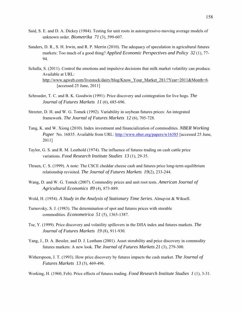
158
Said, S. E. and D. A. Dickey (1984). Testing for unit roots in autoregressive-moving average models of
unknown order. Biometrika 71 (3), 599-607.
Sanders, D. R., S. H. Irwin, and R. P. Merrin (2010). The adequacy of speculation in agricultural futures
markets: Too much of a good thing? Applied Economic Perspectives and Policy 32 (1), 77-94.
Schalla, S. (2011). Control the emotions and impulsive decisions that milk market volatility can produce. Available at URL: http://www.agweb.com/livestock/dairy/blog/Know_Your_Market_281/?Year=2011&Month=6. [accessed 25 June, 2011]
Schroeder, T. C. and B. K. Goodwin (1991). Price discovery and cointegration for live hogs. The Journal of Futures Markets 11 (6), 685-696.
Streeter, D. H. and W. G. Tomek (1992). Variability in soybean futures prices: An integrated
framework. The Journal of Futures Markets 12 (6), 705-728.
Tang, K. and W. Xiong (2010). Index investment and financialization of commodities. NBER Working Paper No. 16835. Available from URL: http://www.nber.org/papers/w16385 [accessed 25 June, 2011]
Taylor, G. S. and R. M. Leuthold (1974). The influence of futures trading on cash cattle price
variations. Food Research Institute Studies 13 (1), 29-35.
Thraen, C. S. (1999). A note: The CSCE cheddar cheese cash and futures price long-term equilibrium
relationship revisited. The Journal of Futures Markets 19(2), 233-244.
Wang, D. and W. G. Tomek (2007). Commodity prices and unit root tests. American Journal of Agricultural Economics 89 (4), 873-889.
Wold, H. (1954). A Study in the Analysis of Stationary Time Series. Almqvist & Wiksell.
Turnovsky, S. J. (1983). The determination of spot and futures prices with storable
commodities. Econometrica 51 (5), 1363-1387.
Tse, Y. (1999). Price discovery and volatility spillovers in the DJIA index and futures markets. The Journal of Futures Markets 19 (8), 911-930.
Yang, J., D. A. Bessler, and D. J. Leatham (2001). Asset storability and price discovery in commodity
futures markets: A new look. The Journal of Futures Markets 21 (3), 279-300.
Witherspoon, J. T. (1993). How price discovery by futures impacts the cash market. The Journal of Futures Markets 13 (5), 469-496.
Working, H. (1960, Feb). Price effects of futures trading. Food Research Institute Studies 1 (1), 3-31.
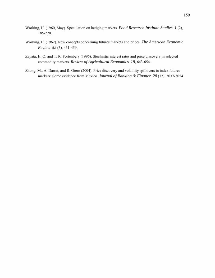
159
Working, H. (1960, May). Speculation on hedging markets. Food Research Institute Studies 1 (2), 185-220.
Working, H. (1962). New concepts concerning futures markets and prices. The American Economic Review 52 (3), 431-459.
Zapata, H. O. and T. R. Fortenbery (1996). Stochastic interest rates and price discovery in selected
commodity markets. Review of Agricultural Economics 18, 643-654.
Zhong, M., A. Darrat, and R. Otero (2004). Price discovery and volatility spillovers in index futures
markets: Some evidence from Mexico. Journal of Banking & Finance 28 (12), 3037-3054.
160
Cheese
Butter
Dry Whey
Nonfat dry milk
Protein Value
Butterfat Value
Other milk solids
Nonfat milk solids
Class III Skim milk
Class IV Skim milk
Class III Milk
Class IV Milk
Note: Surveyed national average cash price of butter is used to infer value of butterfat. Protein value is calculated using survey price of cheese and imputed value of butterfat. Other milk solids are imputed from surveyed cash price for dry whey, and nonfat milk solids are imputed from surveyed cash nonfat dry milk price. Class IV skim milk price is obtained from imputed nonfat milk solids. Class IV milk price is obtained from imputed butterfat value and class IV skim milk value. Imputed other milk solids and imputed protein value are used to calculate class III skim milk price. Finally, class III skim milk price together with imputed butterfat value give us Class III milk price.
Figure 3.1. Flowchart Diagram of Classified Milk Pricing in Federal Milk Marketing Orders
159
161
Cheese
Butter Futures
Dry Whey Cash
Nonfat Dry Milk Cash
Protein Value
Nonfat milk solids
Class III Skim milk
Class IV Skim milk
Class III Milk Futures
Class IV Milk Futures
Regression
Note: Butter futures are used to infer butterfat value. Class IV milk futures and implied butterfat values are used to infer implied values of nonfat milk solids. Class III milk futures and implied butterfat value are used to obtain the implied Class III skim milk price. Implied nonfat milk solids price and projection coefficients obtained using past nonfat dry milk to dry whey cash price ratios are used to obtain fitted other milk solids. Correlations between nonfat milk solids and other milk solids is 0.77. Combining Class III skim milk and other milk solids give us protein price. Finally, butterfat value and protein value give a best guess of implied futures cheese prices.
Butterfat Value
Other milk solids
Figure 3.2. Calculating Implied Cheese Futures Price
160

162
Figure 3.3. Implied vs. Observed Cheese Futures
Note: Three different methods were used to calculate cheese futures price implied from other dairy futures prices.
1. ICF-BDEL (7/11/2000-9/19/2005) uses deliverable butter, and Class III and IV milk futures prices as well as forecasted ratio of nonfat dry milk to dry whey.
2. ICF-BCASH (9/20/2005-3/20/2007) is similar to ICF-BDEL, but cash-settled butter is used instead of deliverable butter.
3. ICF-WHEY (3/21/2007-8/3/2010) uses Class III, cash-settled butter and dry whey futures prices.
4. CHEESE-FUT (8/4/2010- ) are observed cash-settled cheese futures prices.
$1.00
$1.20
$1.40
$1.60
$1.80
$2.00
$2.20
$2.40
ICF-BCASH ICF-WHEY CHEESE-FUT ICF-BDEL

163
Figure 3.4. Average Absolute Value of Cheese Cash-Futures Spread, as a Function of Time to Maturity.
$0.00
$0.05
$0.10
$0.15
$0.20
$0.25
$0.30
$0.35
$0.40
$0.45
$0.50
$0.55
$0.60
510 480 450 420 390 360 330 300 270 240 210 180 150 120 90 60 30
Ave
rage
Abs
olut
e S
prea
d (C
ash-
Fut
ures
)
Trading Days to Maturity
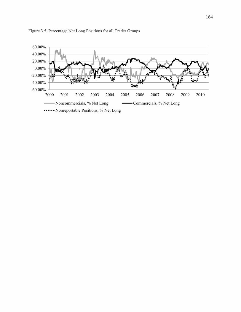
164
Figure 3.5. Percentage Net Long Positions for all Trader Groups
-60.00%
-40.00%
-20.00%
0.00%
20.00%
40.00%
60.00%
2000 2001 2002 2003 2004 2005 2006 2007 2008 2009 2010
Noncommercials, % Net Long Commercials, % Net Long
Nonreportable Positions, % Net Long
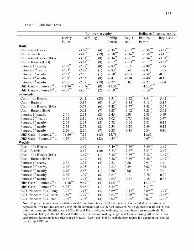
165
Table 3.1. Unit Root Tests
Note: Reported numbers are t-statistics used for unit-root tests. In all tests, intercept is included in the estimated regression. Unit-root test are run using inbuilt commands of RATS 8.01 software. Null hypothesis in all tests is that unit root is present. Significance at 10%, 5% and 1% is indicated with one, two, and three stars respectively. For augmented Dickey-Fuller (ADF) and Phillips-Perron tests optimal lag length is determined using AIC criteria. For cash prices, deseasonalized series is used in tests. “Reg t-stat” is the t-statistic from regression equation that should be used in ADF test.
Rollover: at expiry Rollover: 3 days to expiry Dickey-
Fuller ADF (lags) Phillips
Perron Reg. t-stat.
Phillips-Perron
Reg. t-stat.
Daily Cash – 40# Blocks -3.67*** (4) -3.35** -3.67*** -3.35*** -3.67*** Cash - Barrels -3.16** (19) -3.58*** -3.16** -3.58*** -3.16*** Cash – 40# Blocks (B/O) -3.81*** (8) -3.34** -3.81*** -3.34** -3.81*** Cash – Barrels (B/O) -3.63*** (8) -3.12** -3.63*** -3.11** -3.63** Futures: 1st nearby -2.87** -2.87** (0) -2.87** 0.15 -2.88** 0.15 Futures: 2nd nearby -2.73* -2.92** (1) -2.83* 0.65 -2.83* 0.65 Futures: 3rd nearby -2.67* -2.55 (1) -2.58* -0.05 -2.58* -0.05 Futures: 4th nearby -2.58* -2.23 (8) -2.41 -0.10 -2.40* -0.10 Futures: 5th nearby -2.35 -2.32 (19) -2.22 0.03 -2.22 0.04 Diff: Cash – Futures 2nd n. -11.36*** -11.36*** (0) -11.36*** -11.36*** Diff: Cash – Futures 5nd n. -4.87*** -5.50*** (2) -5.19*** -5.19*** Sales-only Cash – 40# Blocks -3.42** (28) -3.31** -3.42** -3.44*** -3.42** Cash – Barrels -3.14** (0) -3.15** -3.14** -3.15** -3.14** Cash – 40# Blocks (B/O) -3.77*** (6) -3.42** -3.77*** -3.42** -3.77*** Cash – Barrels (B/O) -3.62*** (7) -3.28** -3.62*** -3.28** -3.62*** Futures: 1st nearby -2.41 -2.53 (2) -2.45 0.91 -2.88** 0.19 Futures: 2nd nearby -2.75* -3.10** (15) -3.02** 0.75 -3.05** 0.57 Futures: 3rd nearby -2.68* -2.63* (5) -2.72* -0.04 -2.81* -0.14 Futures: 4th nearby -2.54 -2.54 (2) -2.54 -0.28 -2.49 -0.12 Futures: 5th nearby -2.26 -2.26 (7) -2.28 -0.38 -2.31 -0.10 Diff: Cash – Futures 2nd n. -13.36*** -7.35*** (15) -13.79*** -11.65*** Diff: Cash – Futures 5nd n. -4.29*** -3.70*** (23) -4.54*** -4.67*** Weekly Cash – 40# Blocks -3.69*** (1) -3.49*** -3.69*** -3.49*** -3.69*** Cash - Barrels -2.67* (10) -3.23** -2.67* -3.23** -2.67* Cash – 40# Blocks (B/O) -3.69*** (1) -3.32** -3.69*** -3.32** -3.69*** Cash – Barrels (B/O) -3.49*** (4) -3.28** -3.49*** -3.28** -3.49*** Futures: 1st nearby -2.31 -3.24** (4) -2.53 0.86 -2.93** 1.11 Futures: 2nd nearby -2.68* -2.95** (1) -2.83* 0.59 -3.02** 0.35 Futures: 3rd nearby -2.70* -2.58* (1) -2.66* 0.06 -2.73* 0.01 Futures: 4th nearby -2.60* -3.39** (8) -2.81* 0.13 -2.78* -0.20 Futures: 5th nearby -2.32 -3.24** (8) -2.64* -0.17 -2.38 -0.38 Diff: Cash – Futures 2nd n. -11.36*** -9.69*** (4) -11.53*** -11.39*** Diff: Cash – Futures 5nd n. -5.35*** -5.66*** (1) -5.54*** -5.37*** COT: Noncom. % OI long -3.91*** -3.15** (3) -3.69*** -3.15** -3.69*** -3.69*** COT: Noncom. % OI short -3.56*** -3.79*** (4) -3.63*** -3.79*** -3.63*** -3.63*** COT: Noncom. % OI net l. -3.06** -3.05** (4) -3.02** -3.05** -3.02** -3.02**
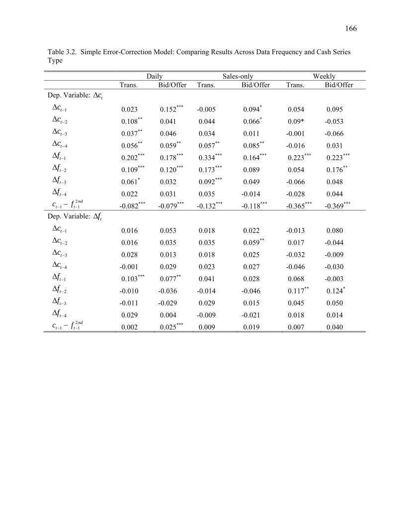
166
Table 3.2. Simple Error-Correction Model: Comparing Results Across Data Frequency and Cash Series Type
Daily Sales-only Weekly Trans. Bid/Offer Trans. Bid/Offer Trans. Bid/Offer
Dep. Variable: tc
1tc 0.023 0.152*** -0.005 0.094* 0.054 0.095 2tc 0.108** 0.041 0.044 0.066* 0.09* -0.053 3tc 0.037** 0.046 0.034 0.011 -0.001 -0.066 4tc 0.056** 0.059** 0.057** 0.085** -0.016 0.031 1tf 0.202*** 0.178*** 0.334*** 0.164*** 0.223*** 0.223*** 2tf 0.109*** 0.120*** 0.173*** 0.089 0.054 0.176** 3tf 0.061* 0.032 0.092*** 0.049 -0.066 0.048 4tf 0.022 0.031 0.035 -0.014 -0.028 0.044 2
1 1nd
t tc f -0.082*** -0.079*** -0.132*** -0.118*** -0.365*** -0.369***
Dep. Variable: tf 1tc 0.016 0.053 0.018 0.022 -0.013 0.080 2tc 0.016 0.035 0.035 0.059** 0.017 -0.044 3tc 0.028 0.013 0.018 0.025 -0.032 -0.009
4tc -0.001 0.029 0.023 0.027 -0.046 -0.030 1tf 0.103*** 0.077** 0.041 0.028 0.068 -0.003 2tf -0.010 -0.036 -0.014 -0.046 0.117** 0.124* 3tf -0.011 -0.029 0.029 0.015 0.045 0.050 4tf 0.029 0.004 -0.009 -0.021 0.018 0.014 2
1 1nd
t tc f 0.002 0.025*** 0.009 0.019 0.007 0.040

167
Table 3.3. Simple Error-Correction Model: Comparing Results Across Data Frequency and Cash Series Type – Log-Prices
Daily Sales-only Weekly Trans. Bid/Offer Trans. Bid/Offer Trans. Bid/Offer
Dep. Variable: tc 1tc 0.036 0.160*** 0.008 0.114*** 0.036 0.098 2tc 0.086** 0.043 0.053** 0.080*** 0.075* -0.039 3tc 0.035** 0.045 0.044 0.016 0.003 -0.045 4tc 0.058*** 0.055** 0.044** 0.074** -0.011 0.025 1tf 0.206*** 0.173*** 0.309*** 0.157*** 0.259*** 0.226*** 2tf 0.110*** 0.119*** 0.164*** 0.068 0.084 0.164** 3tf 0.059** 0.038 0.086** 0.046 -0.059 0.029 4tf 0.053 0.043 0.045 0.000 -0.004 0.063 2
1 1nd
t tc f -0.081*** -0.075*** -0.129*** -0.111*** -0.351*** -0.360***
Dep. Variable: tf 1tc 0.013 0.054* 0.014 0.032 0.000 0.092* 2tc 0.021 0.024 0.051** 0.062*** 0.008 -0.038 3tc 0.029* 0.015 0.021 0.027 -0.022 -0.003
4tc -0.006 0.026 0.013 0.021 -0.039 -0.024 1tf 0.098*** 0.070** 0.048 0.025 0.059 -0.017 2tf 0.000 -0.021 -0.024 -0.055 0.113** 0.108* 3tf -0.019 -0.034 0.029 0.015 0.052 0.050 4tf 0.041* 0.017 -0.004 -0.014 0.033 0.029 2
1 1nd
t tc f 0.004 0.025*** 0.010 0.023* 0.014 0.050

168
Table 3.4. Volatility Spillovers
Price levels Weekly Trans. Bid/Offer Mean Model Dep. Variable: tc 2
1 1nd
t tc f -0.349*** -0.336*** Dep. Variable: tf 2
1 1nd
t tc f 0.049** 0.057** Variance Model: ARCH 11 0.104* -0.202* 12 -0.464*** -0.495*** 21 -0.396*** 0.142 22 0.572*** 0.639*** GARCH 11 0.977*** 0.851*** 12 0.300*** -0.010 21 -0.059 0.182*** 22 0.640*** 0.929*** Likelihood Unrestricted 1877.1 1948.7
1
GRE
t tf c 1821.5*** 1907.1***
1
GRE
t tc f 1849.5*** 1909.9***
Average volatility spillover (% of c. var.)
1t tf c -8.27% 15.72%
1t tc f 27.07% 10.45%
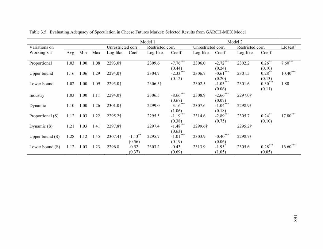
169
Table 3.5. Evaluating Adequacy of Speculation in Cheese Futures Market: Selected Results from GARCH-MEX Model
Model 1 Model 2 Variations on Working’s T
Unrestricted corr. Restricted corr. Unrestricted corr. Restricted corr. LR test§ Avg.
Min Max Log-like. Coef. Log-like. Coeff. Log-like. Coeff. Log-like. Coeff.
Proportional 1.03 1.00 1.08 2293.0† 2309.6 -7.76***
(0.44) 2306.0 -2.72***
(0.24) 2302.2 0.26**
(0.10) 7.60***
Upper bound 1.16 1.06 1.29 2294.0† 2304.7 -2.33***
(0.12) 2306.7 -0.61***
(0.20) 2301.5 0.28**
(0.13) 10.40***
Lower bound 1.02 1.00 1.09 2295.0† 2306.5† 2302.5 -1.05***
(0.06) 2301.6 0.30***
(0.11) 1.80
Industry 1.03 1.00 1.11 2294.0† 2306.5 -8.66***
(0.67) 2308.9 -2.66***
(0.07) 2297.0†
Dynamic 1.10 1.00 1.26 2301.0† 2299.0 -3.16***
(1.06) 2307.6 -1.04***
(0.18) 2298.9†
Proportional (S) 1.12 1.03 1.22 2295.2† 2295.5 -1.19*** (0.38)
2314.6 -2.89***
(0.75) 2305.7 0.24**
(0.10) 17.80***
Dynamic (S) 1.21 1.03 1.41 2297.8† 2297.4 -1.48***
(0.63) 2299.6† 2295.2†
Upper bound (S) 1.28 1.12 1.45 2307.4† -1.13**
(0.56) 2295.7 -1.01***
(0.19) 2303.9
-0.40***
(0.06) 2298.7†
Lower bound (S) 1.12 1.03 1.23 2296.8 -0.52 (0.37)
2303.2 -0.43 (0.69)
2313.9 -1.95*
(1.05) 2305.6 0.28***
(0.05) 16.60***
168
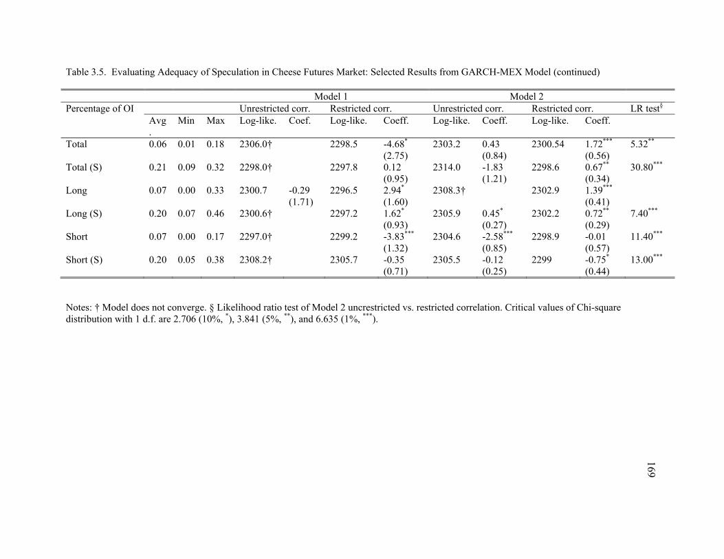
170
Table 3.5. Evaluating Adequacy of Speculation in Cheese Futures Market: Selected Results from GARCH-MEX Model (continued) Model 1 Model 2 Percentage of OI Unrestricted corr. Restricted corr. Unrestricted corr. Restricted corr. LR test§
Avg.
Min Max Log-like. Coef. Log-like. Coeff. Log-like. Coeff. Log-like. Coeff.
Total 0.06 0.01 0.18 2306.0† 2298.5 -4.68* (2.75)
2303.2 0.43 (0.84)
2300.54 1.72***
(0.56) 5.32**
Total (S) 0.21 0.09 0.32 2298.0† 2297.8 0.12 (0.95)
2314.0 -1.83 (1.21)
2298.6 0.67** (0.34)
30.80***
Long 0.07 0.00 0.33 2300.7 -0.29 (1.71)
2296.5 2.94* (1.60)
2308.3† 2302.9 1.39***
(0.41)
Long (S) 0.20 0.07 0.46 2300.6† 2297.2 1.62* (0.93)
2305.9 0.45* (0.27)
2302.2 0.72**
(0.29) 7.40***
Short 0.07 0.00 0.17 2297.0† 2299.2 -3.83***
(1.32) 2304.6 -2.58***
(0.85) 2298.9 -0.01
(0.57) 11.40***
Short (S) 0.20 0.05 0.38 2308.2† 2305.7 -0.35(0.71)
2305.5 -0.12 (0.25)
2299 -0.75*
(0.44) 13.00***
Notes: † Model does not converge. § Likelihood ratio test of Model 2 uncrestricted vs. restricted correlation. Critical values of Chi-square distribution with 1 d.f. are 2.706 (10%, *), 3.841 (5%, **), and 6.635 (1%, ***).
169
Recommended