1
www.crewes.org
Introduction
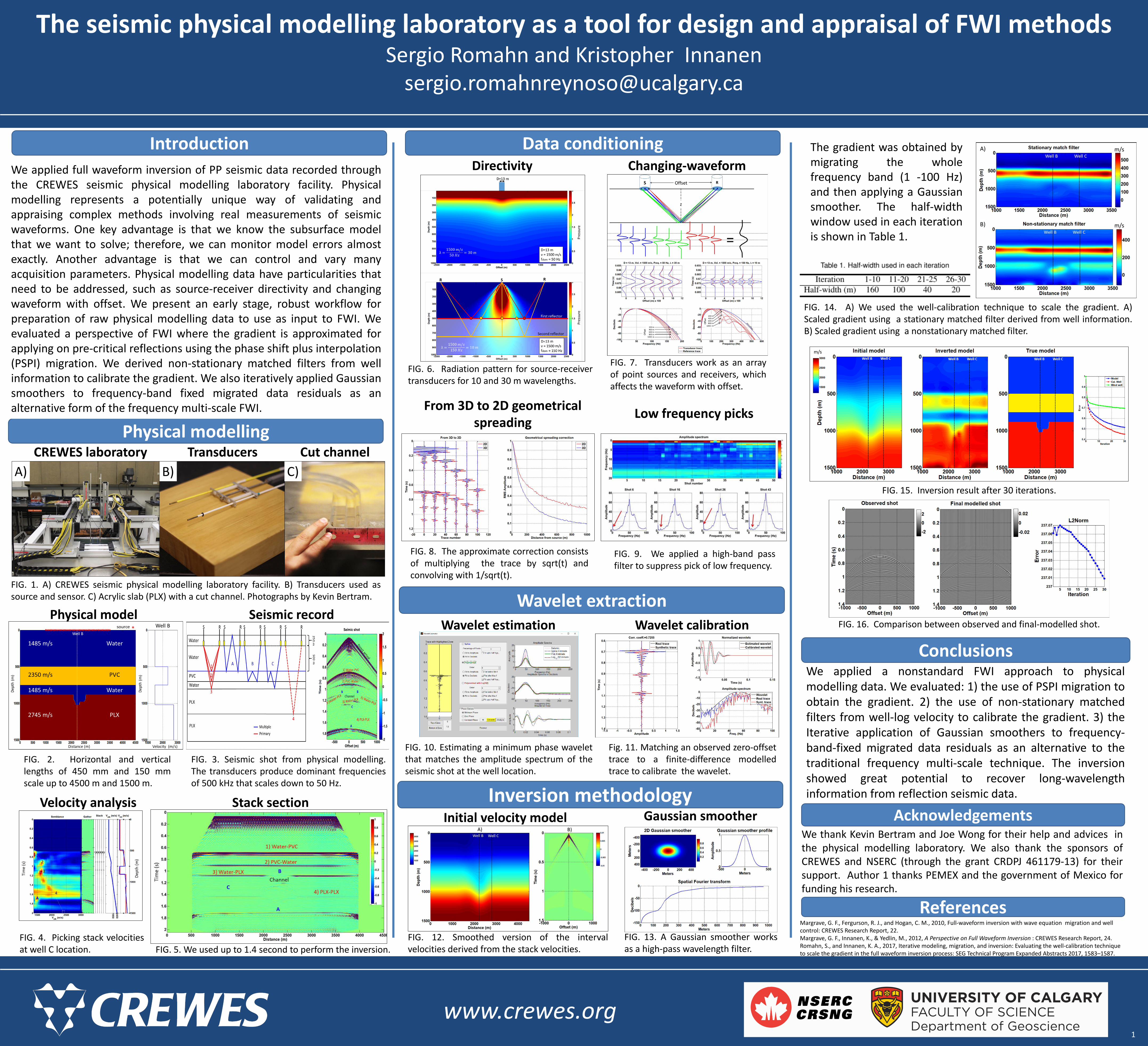
The seismic physical modelling laboratory as a tool for design and appraisal of FWI methodsSergio Romahn and Kristopher Innanen
Conclusions
References
We applied a nonstandard FWI approach to physicalmodelling data. We evaluated: 1) the use of PSPI migration toobtain the gradient. 2) the use of non-stationary matchedfilters from well-log velocity to calibrate the gradient. 3) theIterative application of Gaussian smoothers to frequency-band-fixed migrated data residuals as an alternative to thetraditional frequency multi-scale technique. The inversionshowed great potential to recover long-wavelengthinformation from reflection seismic data.
Margrave, G. F., Fergurson, R. J., and Hogan, C. M., 2010, Full-waveform inversion with wave equation migration and well control: CREWES Research Report, 22. Margrave, G. F., Innanen, K., & Yedlin, M., 2012, A Perspective on Full Waveform Inversion : CREWES Research Report, 24. Romahn, S., and Innanen, K. A., 2017, Iterative modeling, migration, and inversion: Evaluating the well-calibration technique to scale the gradient in the full waveform inversion process: SEG Technical Program Expanded Abstracts 2017, 1583–1587.
AcknowledgementsWe thank Kevin Bertram and Joe Wong for their help and advices inthe physical modelling laboratory. We also thank the sponsors ofCREWES and NSERC (through the grant CRDPJ 461179-13) for theirsupport. Author 1 thanks PEMEX and the government of Mexico forfunding his research.
Directivity
Physical modelling
FIG. 1. A) CREWES seismic physical modelling laboratory facility. B) Transducers used assource and sensor. C) Acrylic slab (PLX) with a cut channel. Photographs by Kevin Bertram.
Data conditioning
Wavelet extraction
From 3D to 2D geometrical spreading
Wavelet estimation
We applied full waveform inversion of PP seismic data recorded throughthe CREWES seismic physical modelling laboratory facility. Physicalmodelling represents a potentially unique way of validating andappraising complex methods involving real measurements of seismicwaveforms. One key advantage is that we know the subsurface modelthat we want to solve; therefore, we can monitor model errors almostexactly. Another advantage is that we can control and vary manyacquisition parameters. Physical modelling data have particularities thatneed to be addressed, such as source-receiver directivity and changingwaveform with offset. We present an early stage, robust workflow forpreparation of raw physical modelling data to use as input to FWI. Weevaluated a perspective of FWI where the gradient is approximated forapplying on pre-critical reflections using the phase shift plus interpolation(PSPI) migration. We derived non-stationary matched filters from wellinformation to calibrate the gradient. We also iteratively applied Gaussiansmoothers to frequency-band fixed migrated data residuals as analternative form of the frequency multi-scale FWI.
FIG. 3. Seismic shot from physical modelling.The transducers produce dominant frequenciesof 500 kHz that scales down to 50 Hz.
FIG. 4. Picking stack velocitiesat well C location. FIG. 5. We used up to 1.4 second to perform the inversion.
Changing-waveform
Low frequency picks
Inversion methodology
Wavelet calibration
Initial velocity model Gaussian smoother
FIG. 6. Radiation pattern for source-receivertransducers for 10 and 30 m wavelengths.
FIG. 7. Transducers work as an arrayof point sources and receivers, whichaffects the waveform with offset.
FIG. 8. The approximate correction consistsof multiplying the trace by sqrt(t) andconvolving with 1/sqrt(t).
FIG. 9. We applied a high-band passfilter to suppress pick of low frequency.
FIG. 10. Estimating a minimum phase waveletthat matches the amplitude spectrum of theseismic shot at the well location.
Fig. 11. Matching an observed zero-offsettrace to a finite-difference modelledtrace to calibrate the wavelet.
FIG. 12. Smoothed version of the intervalvelocities derived from the stack velocities.
FIG. 13. A Gaussian smoother worksas a high-pass wavelength filter.
The gradient was obtained bymigrating the wholefrequency band (1 -100 Hz)and then applying a Gaussiansmoother. The half-widthwindow used in each iterationis shown in Table 1.
FIG. 14. A) We used the well-calibration technique to scale the gradient. A)Scaled gradient using a stationary matched filter derived from well information.B) Scaled gradient using a nonstationary matched filter.
FIG. 15. Inversion result after 30 iterations.
FIG. 16. Comparison between observed and final-modelled shot.
CREWES laboratory Cut channel TransducersA) B) C)
FIG. 2. Horizontal and verticallengths of 450 mm and 150 mmscale up to 4500 m and 1500 m.
Physical model Seismic record
Stack sectionVelocity analysis
Recommended