Geophys. 1. Int. (1993) 112, 39-66

Seismic modelling of subduction zones with inhomogeneity and anisotropy-I. Teleseismic P-wavefront tracking J-M. Kendall" and C. J. Thomson Department of Geological Sciences, Queen's University, Kingston, Ontario, K7L 3N6, Canada

Accepted 1992 July 9. Received 1992 July 8; in original form 1992 March 5

SUMMARY Traveltimes and amplitudes for P-waves from a 500 km-deep source in the Kuril subduction zone have been synthesized by ray tracing in smooth 3-D models that allow general anisotropy and inhomogeneity. The aim is to compare the effects of proposed anisotropy in or near slabs with those of lateral heterogeneity alone. To concentrate on these effects, the source position, slab thickness (90 km), dip (63") and velocity anomaly (5 per cent) are held constant. Results are presented for isotropic models with slab penetration to 670 km and lo00 km. Anisotropic models with 670 km-deep slabs have anisotropy within the slab (Anderson 1987) and in a 10" wedge above the slab (Ribe 1989a; McKenzie 1979). The resulting wavefront topology is never as simple as that in a laterally homogeneous reference Earth and there is strong model dependence of shadow zones, caustics and areas of multipathing.

Rays are traced through slab models defined by 3-D cubic-spline interpolation of up to 21 elastic constants. Outside the slab region, l-D ray tracing through PREM and spherical trigonometry are used to complete the ray path. The results illustrate the importance of using both traveltime and amplitude information when inter- preting slab structure from teleseismic data. Some anisotropic slab models have been found which produce large (>2 s) traveltime residuals that are similar in many parts of the world to those for the deep isotropic model, but the amplitude patterns are substantially different. The model with a deep isotropic slab produces a narrow band of large traveltime residuals (3s) and high amplitudes in a region across northern Canada. This feature is due to the focusing of rays that have travelled down the high-velocity core of the deep slab. Regions where ray theory fails (i.e. caustics) are obvious through multipathing and amplitude singularities. Hilbert- transforms and Airy-type decay caustics should be observed in many places if the models presented are good representations of the Earth. Multipathing in along- strike regions is a pervasive feature of the models considered and the degree of such multipathing is highly dependent on the nature of the slab-boundary velocity gradients. The model with anisotropy above the slab produces multipathing (traveltime triplication) in the down-dip region (i.e. a narrow region through Europe). Identifying such non-linear or 'catastrophic' features in teleseismic data is potentially more diagnostic than linearized interpretations (automated inversion). Overall, the results show that a range of conservative models representing a range of structural theories can encompass a wide range of wavefront consequences.

Key words: anisotropy, caustics, inhomogeneity, multipathing, ray theory, subduc- tion zones, wavefront modelling.

incorporating current petrological and seismological theories. These synthetics would guide the collection and analysis of seismic observations and the testing of geological hypotheses. Indeed, the number of factors influencing real

1 INTRODUCTION

One approach to the question of subduction-zone structure is to create synthetic seismograms for a range of models

data, the spatial sampling that can be reasonably achieved and the global scale of the problem, make the task Seem daunting without some ability to explore the range of

*Now at: Institute of Geophysics and Planetary Physics, Scripps Institution of Oceanography, University of California, San Diego, La Jolla, California, 92093, USA.

14

40 J-M. Kendall and C. J . Thomson

possible effects slabs can have on recordings at a given teleseismic station. A short literature review such as that below leads quickly to the conclusion that anisotropy as well as lateral variability must be included in the models and the computation of synthetic waveforms soon involves many interesting questions on wave propagation theory as well as practical computing problems. For body waves, though, the shape of the wavefront plays a central, sometimes decisive, role in determining the waveforms. As a first step therefore, results of ray tracing through several plausible 3-D models of a subduction zone embedded in an otherwise standard Earth model are presented. For brevity only lower-mantle- turning P-waves and only broad trends for teleseismic arrivals at all azimuths are examined. Strong amplitude variations, multipathing, caustics and shadows are more common than anticipated. Although the slab models presented here are designed to reflect a range of current geological theories, their geometry is rather generic. The results do show quite clearly, though, that wavefronts are very significantly affected by reasonable estimates of the structure. These ray tracing results also provide a framework for addressing theoretical problems concerning the waveforms, which will be pursued in subsequent papers. It is logical to understand first the wavefront geometry effects produced by slabs before addressing the waveform effects (and the required waveform theories).

Studies of seismological data from earthquakes in subduction zones have provided evidence of deep slab penetration (e.g. Creager & Jordan 1984) and subduction region anisotropy (e.g. Ando, Ishikawa & Yamazaki 1983). The latter has been inferred from observed azimuthal variations in P- and S-wave velocities and apparent shear wave birefringence. Ando et al. (1983) observed shear wave splitting from intermediate depth and deep earthquakes beneath Japan. Anisotropy was constrained to a 100km- thick region in the upper-mantle wedge between the slab and lithosphere. Fukao (1984) observed shear wave birefringence in ScS-phases from a deep earthquake in the Kuril slab which was recorded in Japan. Bowman & Ando (1987) observed S-wave splitting and pulse broadening from deep earthquakes in the Tonga subduction zone and, like Ando et al. (1983), anisotropy appeared to be constrained to the upper-mantle wedge. It was also suggested that the observed effects could have been due to multipathing in conjunction with anisotropy. Anisotropy within the slab has been inferred from early P-wave traveltime arrivals for rays travelling in the plane perpendicular to the strike of subduction. Olivine alignment within the slabs beneath the Izu-Manana Island arc (Sugimura & Uyeda 1966) and the Aleutian arc (Cleary 1967) was cited as the cause of anisotropy. More recently, Xie (1991) has inferred anisotropy in the upper portion of the Mariana slab based on observed shear wave splitting. These interpretations are based on isolated observations at specific stations. Wavefront modelling would provide a valuable tool for predicting waveform effects at specific stations.

Considerations of mantle-rock fabric and mineralogy suggest that anisotropy is to be expected. Anisotropy in a wedge-shaped region above the slab has been predicted using models of olivine crystal alignment due to flow-induced deformation at the slab (McKenzie 1979; Ribe 1989a). Subduction-zone pressure and temperature condi-

tions led Anderson (1987) to argue that below 500 km the ilmenite-structure phase of pyroxene will be stable, and that high uniaxial stresses in this region will cause strong anisotropy within the slab. This will be discussed more fully in section 2.

Anomalously large S- and P-wave traveltime residuals from events in the western Pacific rim have been attributed to slab penetration below 1000 km (Jordan 1977; Creager & Jordan 1984, 1986; Fischer, Jordan & Creager 1988). Suetsugu (1989) inverted traveltime residuals to obtain a P-velocity model that suggests the Kuril slab descends to a depth of 1200 km. This result was further strengthened by an analysis of amplitude data. Ray tracing led Silver & Chan (1986) to believe that observed S-wave pulse broadening may also be attributed to deep slab penetration (see below). Some support for lower-mantle slab penetration in certain subduction regions has come from tomographic studies (van der Hilst et al. 1991; Fukao, Obayashi & Inoue 1992). Slab penetration below the 670 km discontinuity would diminish support for two-layer mantle convection theories (Silver, Carlson & Olson 1988) and Anderson (1987) has proposed that the traveltime residuals observed by Creager & Jordan (1984, 1986) may be due to slab anisotropy. In fact Zhou, Anderson & Clayton (1990) have shown that interpreting slab structure from residual sphere analyses can be misleading. The geological significance of subduction-region anisotropy and lower-mantle slab penetration and their potential confusion in seismic interpretation suggest the need for quite general 3-D modelling of subduction zones with these features.

A summary of much of the recent seismic modelling in subducted slabs is given by Engdahl, Vidale & Cormier (1989) and it is clear that there are numerous approaches to the task. Tracking wavefronts and their amplitudes in inhomogeneous elastic media, such as subduction zone models, involves solving the non-separable wave equation. This can be accomplished using a number of techniques, each having its own advantages and disadvantages. Numerical solutions of the wave equation in slab models have been obtained using finite difference calculations (Vidale 1987; Witte 1987; Vidale & Garcia-Gonzalez 1988). Models have been restricted to two dimensions, because the calculations are computationally intensive. It is argued that an advantage of such calculations is that they give very ‘complete’ solutions. Such complete solutions, however, can complicate the interpretation of results because isolation of the effects of specific model attributes can be difficult. This will be best discussed at a later date, when controlled experiments are at hand and the meaning of complete and incomplete is well defined. Certainly there is a need to have at least two independent ways to produce synthetic seismograms for a given physical wave problem.

Local or asymptotic techniques are relatively fast computationally, although this in itself is not the only reason for using ray theory as a starting point. Even if it were possible to calculate waveforms in a reasonable amount of time using numerical methods for 3-D anisotropic media, ray theory and the associated local analysis would still be useful because it provides a way of determining the relationships between the waveforms and model attributes (ke. it is an interpretational tool). For toth isotropic (Cerveng & Ravindra 1971) and anisotropic (Cervenf 1972)

Subduction -zone modelling 4 1

cases, asymptotic ray theory (ART) is appropriate for high-frequency body waves in laterally inhomogeneous media. ART has been used previously to calculate traveltimes and ray paths for isotropic subduction models. In most cases the slab velocity was based on a thermal model developed by Minear & Toksoz (1970) and Toksoz, Minear & Julian (1971) (Sleep 1973; Fujita, Engdahl & Sleep 1981; Rogers 1982; Creager & Jordan 1984, 1986; Silver & Chen 1986; Nieman, Fujita & Rogers 1986). The Julian & Gubbins (1977) ray tracer or an earlier version (Julian 1970) was often used (all of the referenced work in the previous sentence, plus Davies & Julian 1972; Ansell & Gubbins 1986; Bock 1987). A notable exception is the ray tracing scheme of Jacob (1970), which was also used by Suyehiro & Sacks (1979) and Huppert & Frolich (1981). In all of the referenced work, with either ray tracer, amplitudes were not calculated in the full sense, although some amplitude assessment was achieved from ray densities and observed multipathing. Suetsugu (1989) calculated amplit- udes for 2-D isotropic slab models using a hybrid method combining a finite element scheme with geometrical optics. Silver & Chan (1986) observed pulse broadening in S-wave data at azimuths subparallel to the strike of the Kuril subduction zone. They attributed this broadening to rnultipathing and used ray tracing results to support this argument. A 1000 km-deep isotropic slab with a bend or kink produced the necessary multipathing and, hence, caustics.

In addition to being incorrect at low freqiencies, ART is not valid for amplitudes, and consequently waveforms, at caustics. The Gaussian beam summation method (GBM) (Cervenv, Popov & PSenEik 1982; Popov 1982) and the Maslov asymptotic method (Chapman & Drummond 1982; Thomson & Chapman 1985, Kendall & Thomson 1992) in effect sum the contributions of several rays in the vicinity of a point and in this way remain valid at caustics. It has been shown that the GBM is equivalent to the Maslov method under certain conditions (Madariaga & Papadimitriou 1985). Maslov waveforms for the subduction-zone models of this paper will be presented in a subsequent paper.

Weber (1990) used the GBM to model P-waves in 2-D subduction zones, systematically exploring the effects of variations in the depth, velocity anomaly, thickness and dip of the slab and variations in the source position. In many cases these variations created small differences in traveltime residuals, but significant differences in magnitude residuals. Although the GBM was used, waveforms were not presented for the modelling results. The work of Weber (1990) has been very helpful in guiding the development of the modelling in this paper. Many of the wavefront features identified by Weber (1990) have been observed in the results presented here, adding confidence in these results. In some ways, this paper is the logical extension of Weber’s work to 3-D models with anisotropy. In this case, though, we have many more parameters which can be varied and it is necessary for us to be restrictive with some of them (e.g. source depth).

Cormier (1989) has used the GBM to model S-waves in 3-D subduction zones. Where possible,, the beam width was made very wide (i.e. beams approach plane waves), in which case the GBM is essentially equivalent to the Maslov method (Madariaga & Papadimitriou 1985). Rays were

traced from the receiver into the source region and receiver waveforms were constructed by assuming reciprocity for the Gaussian beam solution. The validity of this technique is not immediately apparent. Support for this approach comes from Nowack & Aki (1984), where GBM waveforms are compared for summation in the receiver region and the source region. For the given examples, the waveforms compared favourably. It is not clear, though, that this approach is valid in cases with complex velocity structures in the source or receiver regions. More theoretical work is required in order to understand reciprocity and its incorporation. Cormier’s (1989) results showed pulse broadening of S-waves throughout the front-of-slab region. This was attributed to a process termed ‘slab diffraction’. Cormier (1989) described low-frequency energy ‘leaking’ out of the slab and travelling in the surrounding slower material. As a result, low frequency energy arrives at the receiver later than the impulsive high-frequency signal, thereby elongating the waveform. Cormier (1989) did not generate waveforms in the along-strike region, due to the complicated wavefront topology. It was found that the slab phase faded quickly as receiver azimuths moved into the back-of-slab region.

Another source of waveform distortion is due to sharp kinks in the wavefront that are a result of strong velocity gradients. Such wavefront kinks will cause low-frequency waveform tail interference. This distortion effect and the diffraction effect (Cormier 1989) will be controlled by the sharpness of the slab-boundary velocity gradients (see section 5.2). A closer study of the physics controlling this effect is needed. Higher-order ray-theory terms (Thomson, Coates & Kendall 1991) or, the related, scattering integral solutions (Coates & Chapman 1990; Cormier 1990; Thomson, Kendall & Guest 1992) and the Maslov method (Kendall & Thomson 1992) can all describe this type of slab-waveform distortion.

A requirement of the Maslov method (or the GBM) is that a sufficient number of rays must be traced in the vicinity of a desired receiver. It is highly likely that there will be regions in the model where the wavefront topology will be quite regular and that there will be no gain in calculating waveforms using the Maslov method over standard ray-theory seismograms. For these reasons, ART should be considered a necessary ‘first pass’ in order to identify regions that require the Maslov method, and indeed other methods, to determine waveforms. Regions where ray theory is not valid (e.g. caustics) are apparent through amplitude singularities, traveltime triplication and multipathing. Monitoring the KMAH index (Chapman & Drummond 1982; Thomson & Chapman 1985; Kendall & Thomson 1992) along ray paths records the passage of rays through caustics and signals that an appropriate waveform modification should be made at the receiver. Such non-linear or ‘catastrophic’ features in teleseismic data are potentially much more diagnostic than linearized traveltime inversion techniques, which assume an almost spherically stratified model and, hence, regular wavefront topology. Understanding the relevant caustics and identifying receiver regions where techniques like the Maslov method must be used for waveforms, is one of the main aims of this paper.

In order to compare the effects of anisotropy with those of inhomogeneity alone, all models have a fixed source depth

42 J - M . Kendall and C. J . Thomson

900-

of 500 km, a slab dip of 63", a velocity anomaly of 5 per cent and a thickness of roughly of YO km. A deep event ensures that the majority of downgoing rays turn below the 670 km discontinuity, thereby avoiding problems associated with upper-mantle P-wave triplication in PREM (Dziewonski & Anderson 1981). More complete descriptions of the models are given in section 2. Rays are first traced through a local subduction-zone model specified in Cartesian coordinates and are then interfaced with the global model PREM using spherical coordinates. Cartesian coordinates are used in the local model because they are most convenient for numerical work with general forms of anisotropy. Details of the anisotropic ray tracing and the interfacing are given in section 3 and appendix A. The event simulated is situated in the Kuril slab, with its epicentre in the Sea of Okhotsk. This source location was chosen because receivers perpendicular to slab strike will lie in Europe and receivers parallel to strike will lie in North America, both good regions of seismograph station coverage. Additionally, the location of this event is similar to those studied by many of the authors referenced above. The strike of the Kuril slab is fairly linear, thus simplifying the modelling of the subduction-zone geometry. It should be noted that the modelling is not limited to such a geometry, but it is a logical starting point.

2 MODEL PARAMETERIZATION

Each subduction-zone structure is defined within a certain box by specifying the elastic constants and density on a 3-D grid of regularly spaced knot points. A modified four-point 3-D cubic spline, written by M. L. Smith, is used to interpolate the elastic constants and density between knots (Thomson & Gubbins 1982). The knot spacing is 50 km in the depth (xg) and strike ( x 2 ) directions and 25 km in the direction perpendicular to strike (xJ. The overall dimensions of the box vary as necessary in the x1 and xg directions and it extends 1000 km in the x2 direction. The structure is only specified at depths greater than 220 km, which is the base of the LID/LVZ zone.

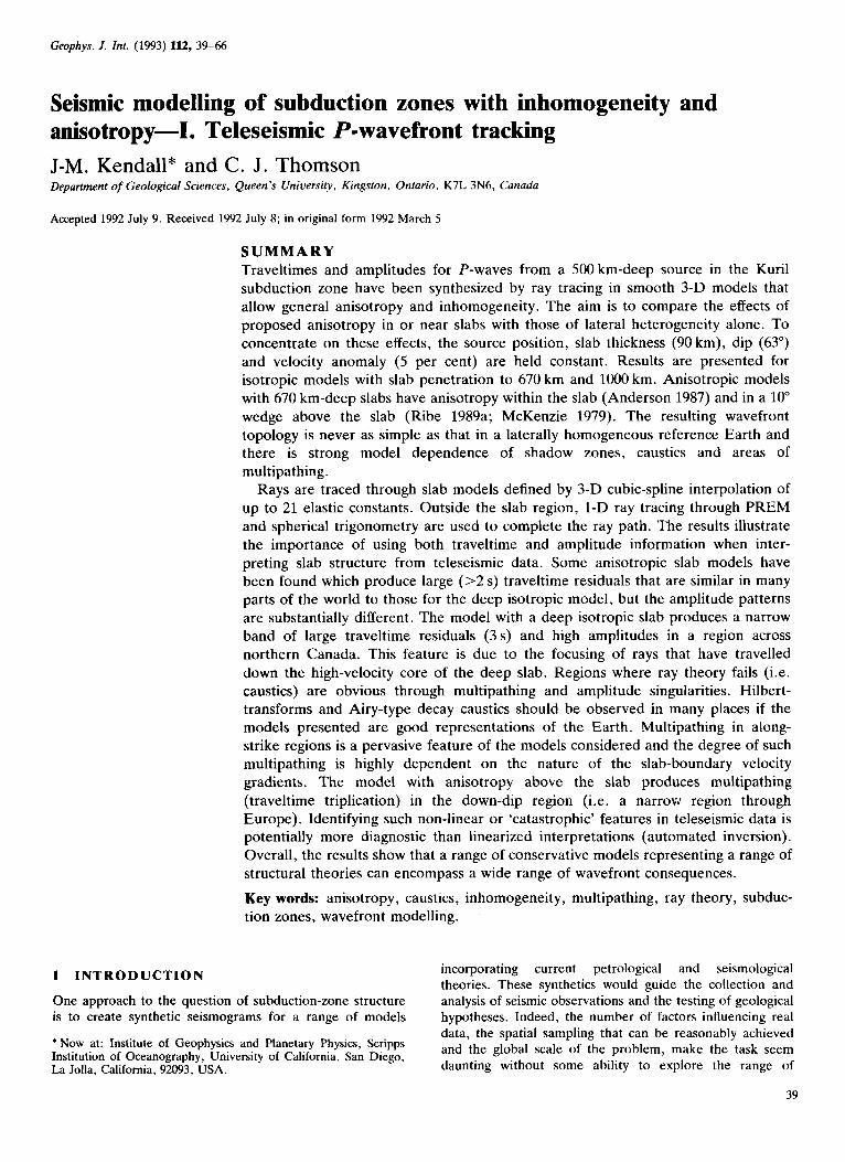
Each of the models considered has a subduction-zone anomaly superimposed on PREM. For simplicity, the ray tracing program used here is for anisotropic, in- homogeneous media without interfaces and the discon- tinuities at 400km and 670km in PREM have been smoothed out within the local model. The PREM values for these discontinuties will be perturbed by the slab in an as yet unclear fashion and it seems unwarranted to introduce extra unknowns to model this, even though there is no theoretical difficulty in the ray tracing (Guest, Spencer & Thomson 1992). The PREM smoothing is accomplished using a 1-D spline interpolation of velocities and densities as a function of radius in the vicinity of 400 km and 670 km. Fig. 1 shows a comparison of PREM and its smoothed version. The effects of the smoothing are small for teleseismic P-waves (see section 4).

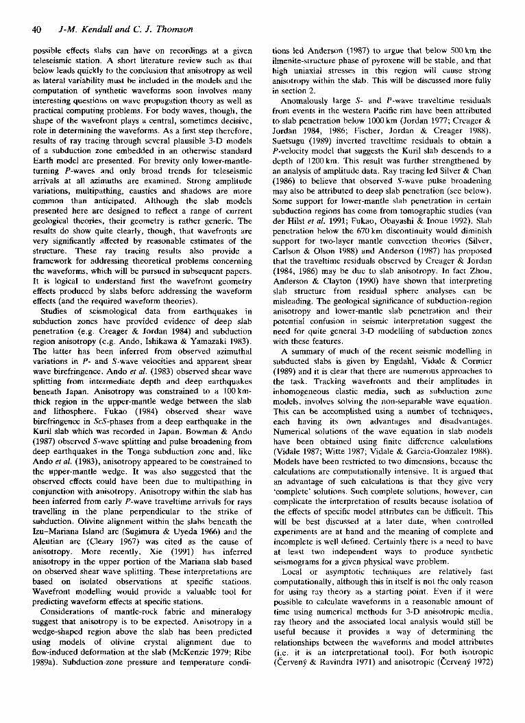
A subducted slab of oceanic lithosphere is superimposed on PREM within the box. The angle of subduction is 63" and the slab thickness is roughly Y0km (Fig. 2). The velocities at knots within the slab are typically increased by 5 per cent over PREM values. Along strike, the slab penetrates to a constant depth (or rather, radius) in the

PREM VELOCITIES 12.0,

actual

5.0

4.0 ' 25 0 450 650 850 1050

Depth (W

Figure 1. The actual P- and S-wave velocities for PREM (Dziewonski & Anderson 1981) are shown in solid lines and the approximated PREM velocities used in the subduction-zone model are shown in dotted lines. For teleseismic signals, the effect of the discontinuity smoothing is very small compared with the effect of the slab anomalies (see section 4).

OFFSET (km) 0 200 400 600

100 63"

0 OLIVINE Q ILMENITE

\ \ PREM

1000 km Y l Figure 2. A cartoon showing the geometry of the subduction-zone models viewed in the plane perpendicular to the strike of subduction. Ellipses and triangles indicate regions that may be anisotropic. The source is indicated by the '+'.

Subduction-zone modelling 43

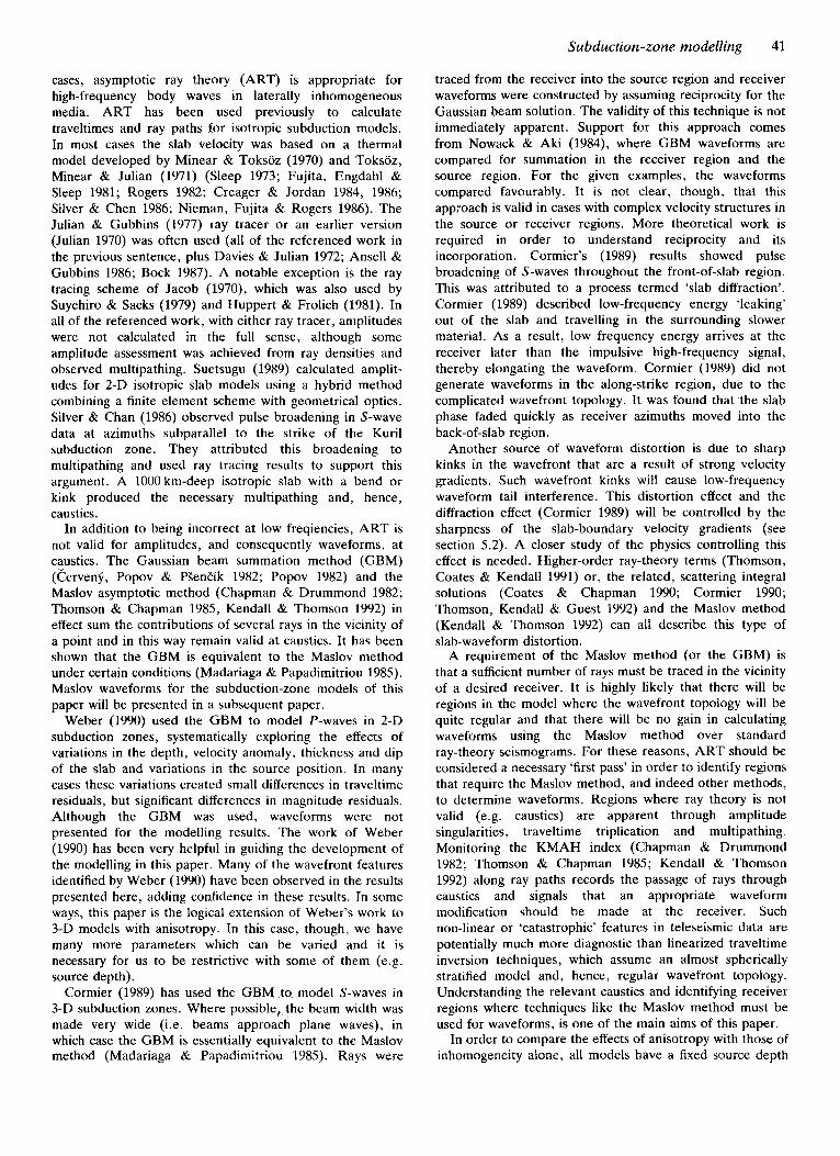
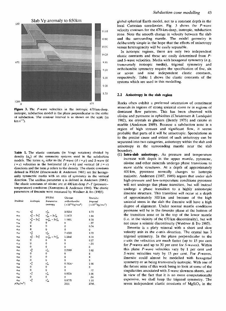
global spherical Earth model, not to a constant depth in the local Cartesian coordinates. Fig. 3 shows the P-wave velocity contours for the 670-km-deep, isotropic, subduction zone. Note the smooth change in velocity between the slab and the surrounding mantle. The model geometry is deliberately simple in the hope that the effects of anisotropy versus heterogeneity will be easily separable.

In isotropic regions, there are only two independent elastic constants and these are easily determined from P - and S-wave velocities. Media with hexagonal symmetry (e.g. transversely isotropic media), trigonal symmetry and orthohombic symmetry require the specification of five, six or seven and nine independent elastic constants, respectively. Table 1 shows the elastic constants of the systems which are used in this modelling.

150

670

1200 0 67

Slab VD anomaly to 650km

1 1 10

10 80

10 50

10 20

9 90

9 60

9 30

9 00

8 70

5

Figure 3. The P-wave velocities in the isotropic 670 km-deep, isotropic, subduction model in the plane perpendicular to the strike of subduction. The contour interval is as shown on the scale (in km s-I).

Table 1. The elastic constants (in Voigt notation) divided by density (ai j ) of the symmetry systems used in the subduction models. The terms u,, refer to the P-wave (if i = p ) and S-wave (if i = s) velocities in the horizontal (if j = h) and vertical (if j = u ) directions and the term p refers to the density. The elastic constants defined in PREM (Dziewonski & Anderson 1981) are for hexago- nally symmetric media with an axis of symmetry in the vertical direction. The unitless parameter 9 is defined in Anderson (1961). The elastic constants of olivine are at 400 km-deep P-T (pressure- temperature) conditions (Kumazawa & Anderson 1969). The elastic parameters of ilmenite were measured by Weidner & Ito (1985).

PREM: Olivine: Ilmenite:

IJOtrOpy (x10”kg/ms2) ( x10”kg/ms2) tnclinic isotropic transverse orthorhombic trigonal

4 v; - 2 4 vf - 2u: 0 0 0

v: v; - 2 4 0 0 0

0 0 0

0 0

0

4

v:

4

4

v;” 0 0 0

0 0

0

4“

4.

3.8214 1.1472 1.1801 0 0 0 2.4233 1.1846 0 0 0 2.7989 0 0 0 0.7554. 0 0 0.8224 0 0.8775 3311.

4.72 1.68 0.70 -.27 0.24 0 4.72 0.70 0.27 -.24 0 3.82 0 0 0 1.06 0 -.27 1.06 -.24 1.52 3795

2.1 Anisotropy in the slab region

Rocks often exhibit a preferred orientation of constituent minerals in regions of strong uniaxial stress or in regions of dominant flow patterns. This has been observed with olivine and pyroxene in ophiolites (Christensen & Lundquist 198Z), ice crystals in glaciers (Bently 1975) and calcite in marble (Anderson 1989). Because a subduction zone is a region of high stresses and significant flow, it seems probable that parts of it will be anisotropic. Speculations as to the precise cause and extent of such anisotropy can be separated into two categories, anisotropy within the slab and anisotropy in the surrounding mantle near the slab boundary. (1) Intra-slab anisotropy. As pressure and temperature

increase with depth in the upper mantle, pyroxene, olivine and other minerals undergo phase transitions to more stable structures. At a depth of approximately 400 km, pyroxene normally changes to isotropic majorite. Anderson (1987, 1989) argues that under slab high-pressure and low-temperature conditions pyroxene will not undergo this phase transition, but will instead undergo a phase transition to a highly anisotropic ilmenite structure. This transition will occur at a depth of approximatefy 500km and because of the high uniaxial stress in the slab the ilmenite will have a high degree of alignment. Under normal mantle conditions pyroxene will be in the ilmenite phase at the bottom of the transition zone or in the top of the lower mantle (i.e. in the vicinity of the 670 km discontinuity), but will not cause a seismic discontinuity (Weidner & Ito 1985).

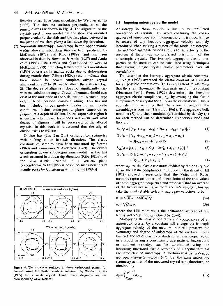
Ilmenite is a platy mineral with a short and slow velocity axis in the c-axis direction. The crystal has 3 trigonal symmetry. In the plane perpendicular to the c-axis the velocities are much faster (up to 15 per cent for P-waves and up to 30 per cent for S-waves). Within this plane P-wave velocities vary by 1 per cent and S-wave velocities vary by 15 per cent. For P-waves, ilmenite could almost be modelled with hexagonal symmetry or as being transversely isotropic. With one of the future aims of this work being to look at some of the singularities associated with S-wave slowness sheets, and in view of the fact that it is no more computationally expensive, we shall keep the trigonal symmetry. The seven independent elastic constants of MgSiO, in the

44 J-M. Kendall and C. J . Thomson

ilmenite phase have been calculated by Weidner & Ito (1985). The slowness surfaces perpendicular to the principle axes are shown in Fig. 4. The alignment of the crystals used in our model has the slow axis oriented perpendicular to the slab and the fast plane oriented in the plane of the slab, giving a fast down-dip direction.

(2) Supra-slab anisotropy. Anisotropy in the upper mantle wedge above a subducting slab has been predicted by McKenzie (1979) and Ribe (1989a) and has been observed in data by Bowman & Ando (1987) and Ando et al. (1983). Ribe (1989a and b) extended the work of McKenzie (1979) predicting lattice-preferred orientation (LPO) of crystals in mantle rocks due to deformation during mantle flow. Ribe's (1989a) results indicate that there should be nearly complete olivine crystal alignment in a 5" to 10" wedge above the slab (see Fig. 2). The degree of alignment does not significantly vary with the subduction angle. Crystal alignment should also exist at the underside of the slab, but not to such a large extent (Ribe, personal communication). This has not been included in our models. Under normal mantle conditions, olivine undergoes a phase transition to @-spinel at a depth of 400 krn. In the supra-slab region it is unclear what phase transitions will occur and what degree of alignment will be preserved in the altered crystals. In this work it is assumed that the aligned olivine exists to 650 km.

Olivine has (2 m 2 m 2 m) orthohombic symmetry with a long a- or fast-axis direction. The elastic constants of samples have been measured by Verma (1960) and Kumazawa & Anderson (1969). The crystal orientation in our subduction zone model has the fast a-axis oriented in a down-dip direction (Ribe 1989a) and the slow b-axis oriented in a vertical plane perpendicular to this [this is based on measurements in mantle rocks by Christensen & Lundquist (1982)l.

JLMEMTE Slowness surfaces ( s h ) x3 x1 x2

0.2

x3 X

-0.2 -0.2 0.2 -0.2 0.2 -0.2 0 .2

Wave surfaces (km/s) x3 x1 x2

11.0

x3 X

11.0 -11.0 11.0 -11.0 11.0 -11.0 11.0

Figure 4. The slowness surfaces in three orthogonal planes for ilmenite using the elastic constants measured by Weidner & Ito (1985) for a single crystal. Lower three diagrams are the corresponding wave surfaces.

2.2 Imposing anisotropy on the model

Anisotropy in these models is due to the preferred orientation of crystals. To avoid confusing the conse- quences of anisotropy and inhomogeneity, it is important to be aware of any isotropic aggregate velocity anomaly introduced when making a region of the model anisotropic. The isotropic aggregate velocity refers to the velocity of the medium if there was no preferred orientation of the anisotropic crystals. The isotropic aggregate elastic pro- perties of the medium can be calculated using techniques that average single crystal elastic parameters over all orientations.

To determine the isotropic aggregate elastic constants, cij, Voigt (1928) averaged the elastic constant of a crystal for all possible orientations. This is equivalent to assuming that the strain throughout the aggregate medium is constant (Hearmon 1961). Reuss (1929) determined the isotropic aggregate elastic compliances, sij, by averaging the elastic compliances of a crystal for all possible orientations. This is equivalent to assuming that the stress throughout the assemblage is constant (Hearmon 1961). The aggregate bulk modulus (K) and shear modulus (G) divided by density ( p ) for each method can be determined (Anderson 1965) and they are:

K v / p = [(ail + a22 + a331 + 2(a12 + a23 + a i J I / 9

G,/P = [(all + a22 + a331 - (a12 + a23 + 0 1 3 )

KRlp = [ ( s ) I ~ + ~ ; 2 + ~ 4 3 ) + 2(~ ;2 + SL + ~i3) I - l

(1)

(2)

(3)

+3(Sh4+S;s+Sk6)]-'> (4)

+ 3(a4, + ass + a,)i/15

GJp = W(S;, +s ; ,+s .~~) - ~ ( s ; ~ + s ; ~ + s ; ~ )

where aii are the elastic constants divided by the density and S; are the elastic compliances multiplied by the density. Hill (1952) showed theoretically that the Voigt and Reuss methods represent upper and lower limits of the true values of these aggregate properties and proposed that an average of the two values will give more accurate results. Thus we take the most reliable isotropic aggregate velocities to be

up = ~ ( K H 4 / 3 G ~ ) / p (5a)

us = m p , (5b) where the Hill modulus is the arithmetic average of the Reuss and Voigt moduli defined by (1-4).

Multiplying the elastic constants and compliances of an anisotropic crystal by a constant will change the isotropic aggregate velocity of the medium, but still preserve the symmetry and degree of anisotropy of the medium. Using this fact, the set of elastic constants for an anisotropic region in a model having a constraining aggregate or background or ambient velocity, can be determined using the laboratory-measured elastic constants of a crystal that has the same class of anisotropy. A medium that has a desired isotropic aggregate velocity (v*), but the same anisotropy symmetry as that of the measured crystal can, therefore, be obtained by

(6a)

Subduction-zone modelling 45

I I,* \ -2

where the * denotes the elastic parameters and velocity of the anisotropic region and xtal denotes those for a measured crystal. Obviously this can only be done for one of the isotropic velocities and we have accordingly chosen the compression velocity to remain unchanged. We emphasize that this procedure is somewhat arbitrary, but it does allow us to exercise some control over the model anomalies. The aggregate background may be chosen to be, for example, the standard PREM velocity for the given depth or a reasonable isotropic slab velocity.

The regions in the subduction zone that may be anisotropic are indicated in Fig. 2. The model of a subduction zone with intra-slab anisotropy has anisotropy attributed to olivine alignment in the range 150 km to 500km depth and ilmenite alignment between the depths 500 km and 650 km. The supra-slab anisotropy model has olivine alignment in a 10" wedge in the mantle above the slab. The elastic constants of Weidner & Ito (1985) are used for ilmenite and those of Kumazawa & Anderson (1969) are used for olivine. In the models, the anisotropic elastic constants are 'blended' with the initial (PREM or slab) isotropic elastic constants of the region. The blending is done such that the degree of crystal alignment can be vaned: the final elastic constants are a weighted average of the isotropic constants and those for a fully-aligned aggregate. Again, this is done to allow us some control over the models without being too complicated.

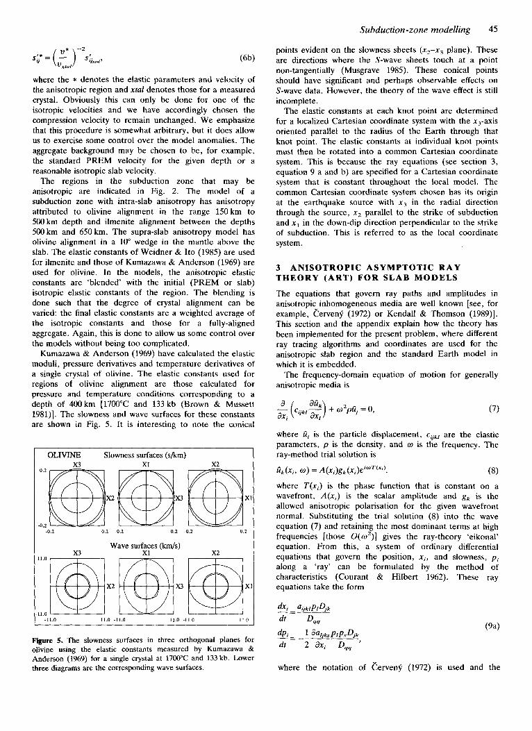
Kumazawa & Anderson (1969) have calculated the elastic moduli, pressure derivatives and temperature derivatives of a single crystal of olivine. The elastic constants used for regions of olivine alignment are those calculated for pressure and temperature conditions corresponding to a depth of 400 km [17WC and 133kb (Brown & Mussett 198l)l. The slowness and wave surfaces for these constants are shown in Fig. 5 . It is interesting to note the conical

OLIVINE, Slowness surfaces (s/km) x3 XI x2

0.2

x3 X

-0.2 -0.2 0.2 -0.2 0.2 -0.2 0.2

Wave surfaces (km/s) x3 x1 x2

11.0

11.0

x2 x3 X

' -11.0 11.0 -11.0 11.0 -11.0 11.0

Figure 5. The slowness surfaces in three orthogonal planes for olivine using the elastic Constants measured by Kumazawa & Anderson (1969) for a single crystal at 1700°C and 133 kb. Lower three diagrams are the corresponding wave surfaces.

points evident on the slowness sheets (x2-x3 plane). These are directions where the S-wave sheets touch at a point non-tangentially (Musgrave 1985). These conical points should have significant and perhaps observable effects on S-wave data. However, the theory of the wave effect is still incomplete.

The elastic constants at each knot point are determined for a localized Cartesian coordinate system with the x,-axis oriented parallel to the radius of the Earth through that knot point. The elastic constants at individual knot points must then be rotated into a common Cartesian coordinate system. This is because the ray equations (see section 3, equation 9 a and b) are specified for a Cartesian coordinate system that is constant throughout the local model. The common Cartesian coordinate system chosen has its origin at the earthquake source with x, in the radial direction through the source, x2 parallel to the strike of subduction and xI in the down-dip direction perpendicular to the strike of subduction. This is referred to as the local coordinate system.

3 ANISOTROPIC ASYMPTOTIC R A Y THEORY (ART) FOR SLAB MODELS

The equations that govern ray paths and amplitudes in anisotropic inhomogeneous media are well known [see, for example, Cerveny (1972) or Kendall & Thomson (1989)]. This section and the appendix explain how the theory has been implemented for the present problem, where different ray tracing algorithms and coordinates are used for the anisotropic slab region and the standard Earth model in which it is embedded.

The frequency-domain equation of motion for generally anisotropic media is

(7)

where ii, is the particle displacement, C&[ are the elastic parameters, p is the density, and w is the frequency. The ray-method trial solution is

Gk(X,, W ) = A(X,)gk(X,)ezWT(Xi). (8) where T(xJ is the phase function that is constant on a wavefront, A @ , ) is the scalar amplitude and g, is the allowed anisotropic polarisation for the given wavefront normal. Substituting the trial solution (8) into the wave equation (7) and retaining the most dominant terms at high frequencies [those 0 ( m 2 ) ] gives the ray-theory 'eikonal' equation. From this, a system of ordinary differential equations that govern the position, x, , and slowness, p l along a 'ray' can be formulated by the method of characteristics (Courant & Hilbert 1962). These ray equations take the form

- dPi - - aaljksPIPsDjk dt 2 ax, Dqq '

where the notation of Cerveny (1972) is used and the

46 J-M. Kendall and C. J . Thomson

cofactor term is defined

Oij = 1/6EiklEjmn(rkrn - bkrn)(rln - (9b) The term r j k = aijklpipI where aijkl = czjkl/p. It can be shown that t is the time along the raypath (Kendall & Thomson 1989). Given a set of initial conditions one can numerically integrate the ray equations and thereby determine the position and slowness at every point on a raypath.

To determine the amplitude of the ray solution, the ray-theory ‘transport’ equation must be used. This equation results from considering frequency terms O( w ) when substituting the trial solution (8) into the wave equation (7). The solution of the transport equation for the magnitude of the displacement, A, is

A = constant ( p ~ ) - t , (10a) where

The constant term depends on the source and must be determined by treating the anisotropic point source problem. This has been considered elsewhere for a homogeneous source region (Kendall, Guest & Thomson 1992).

When the determinant of partial derivatives, J, equals zero, the amplitude is singular and asymptotic ray theory will no longer be valid. This is exactly what happens in regions where the raypaths cross and form a ‘caustic’. At the caustic the Maslov method must be used to determine waveforms. Fortunately the failure is local and ray theory is valid when tracking a ray through one of these regions. Each time a ray passes through a caustic the sign of J changes and the KMAH index, in most cases, increases by one (Chapman & Drummond 1982; Thomson & Chapman 1985; Kendall & Thomson 1992). Monitoring the KMAH index along the ray specifies the appropriate number of Hilbert transforms to be applied to the waveform at the receiver.

It is evident from (lob) that the partial derivatives of the ray paths with respect to the initial parameters are required. The corresponding geometrical spreading equations are obtained by differentiating the ray equations (9) with respect to the initial parameters or ray coordinates, ar,

where

These are a system of 18 ordinary differential equations and,

as with the ray equations, they can be numerically integrated given a set of initial conditions. The initial conditions used in this work are those for a point source which are given explicitly in Kendall & Thomson (1989). To reduce computation time these equations are reduced to a system of 12 by using the time along the ray and the initial ray take-off angles as ray coordinates (Cerveny 1972).

Equations (9) and (11) are used to trace a ray within a generally inhomogeneous and anisotropic subduction region specified in Cartesian coordinates. When the ray has left the local Cartesian model it is continued to teleseismic distances through the background model PREM (Dziewon- ski & Anderson 1981) using a ray tracer for spherically symmetric media specified in spherical coordinates (de- scribed in Kendall 1991). This ray tracer is much simpler and computationally faster than that used within the slab region (i.e. simpler than that for generally anisotropic inhomogeneous media). The wavefront information at the final point on a ray in the local Cartesian model must serve as the ‘initial conditions’ for the ray to be continued through the global model. This necessitates transforming the Cartesian-coordinate wavefront information into global spherical coordinates. These matching-point ‘initial condi- tions’ are, of course, quite different to those for a point source. Care must be taken to transform correctly all of the geometrical spreading factors of the ray that leaves the local model and continues into PREM. Partial derivatives of the final teleseismic location and slowness, with respect to initial conditions at the source, must be obtained so that the final ray amplitude can be found using (10). The details of continuing a ray from the local Cartesian model through the spherical model and the necessary matching calculations are algebraically quite tedious and are therefore given in the Appendix.

Numerous checks have been done to assess the accuracy of the ray tracing scheme described above. To check the interfacing calculation, rays were traced through a local model without a slab anomaly and then interfaced with the global model PREM. The results were in close agreement with those for rays traced solely in the global model. Calculations of the geometrical spreading (lob) were cross-checked Tising simple finite differencing schemes to evaluate the d x , / d a , terms. Finally, the knot spacing used in the model parameterization and the time step used the numerical integration of (9) and (11) were varied to assure stability in the results. Varying the knot spacing is important to assure that the spline interpolation is not introducing oscillations in the elastic constants between nodes. This can be a problem in regions where there are sharp gradients in the elastic constants.

4 WAVEFRONT PREDICTIONS

In this section the results of tracing P-waves in six plausible subduction-zone models are presented. Two isotropic models are discussed, one with a slab penetrating the mantle to the 670 km discontinuity and the other with a slab penetrating to a depth of 1000 km (i.e. well into the middle mantle). Four anisotropic models are considered: one with anisotropy in a wedge-shaped region above the slab, one with anisotropy within a high-velocity slab, one with

Subduction-zone modelling 47

anisotropy within a slab with no aggregate velocity anomaly (see section 2) relative to PREM, and the last one has a combination of anisotropy within and above a high-velocity slab. These six models span a range of structures consistent with the current theories outlined above, but they are by no means exhaustive. The intent of using these models is to identify a corresponding range of possible P-wavefront effects.

Rays were traced from a 500 km-deep source located in the centre, with respect to both the strike and perpendicular-strike directions, of the slab. In each model, rays leave the source with take-off angles from the radial direction varying from 120" to 240" at 0.5" increments (0" is the direction towards the surface of the Earth). Azimuthal take-off angles were measured from the direction perpen- dicular to the strike of subduction and varied from 0" to 355" in 5" increments (0" is the down-dip direction perpendicular-strike of the subduction zone, also referred to as x 1 above). Additional rays were traced in regions where more resolution was needed because of complicated wavefront distortion. Rays that turned above or were reflected at the 670-km discontinuity were discarded in order to avoid problems associated with traveltime triplications in PREM in the 15" to 30" range. All rays were traced to a depth greater than 700 km in the local model before being matched with the global ray tracer. This ensured that any (small) influence of the approximation of PREM around the 670 km discontinuity was consistently present for all rays traced. Additionally, rays were only allowed to interface with the global PREM model when the velocity difference between the local and global models at the point of matching was less than 0.1 per cent. This ensured that the rays had left anomalous (relative to PREM) velocity

3) 0.

-1.

- 2 .

- 3 .

TRAVEL-TIME RESIDUALS ~--LUO...~~~~..01.HI..." . .

0 degree plane

* deep * supra X intra-A *

background * degrees from epicentre *

20 30 40 50 60 70 80 90 100

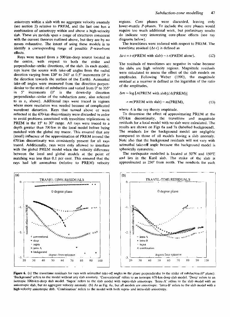
regions. Core phases were discarded, leaving only lower-mantle P-phases. To include the core phases would require too much additional work, but preliminary results do indicate very interesting core-phase effects (see ray diagrams below).

The traveltimes were reduced with respect to PREM. The traveltime residual (At-t) is defined as

At-t = t-t(PREM with slab) - t-t(PREM alone). (12)

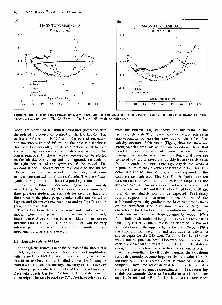
The residuals of traveltimes are negative in value because the slabs are high velocity regions. Magnitude residuals were calculated to assess the effect of the slab models on amplitudes. Following Weber (1990), the magnitude residual at a receiver is defined as the logarithm of the ratio of the amplitudes,

Am = log [A(PREM with slab)/A(PREM)]

= m(PREM with slab) - rn(PREM), (13)

where A is the ray theory amplitude. To determine the effect of approximating PREM at the

670-km discontinuity, the traveltime and magnitude residuals for a local model with no slab were calculated. The results are shown on Figs 6a and 7a (labelled background). The residuals for the background model are negligible compared to those of all models having a slab anomaly. Note also that the background residuals will not vary with azimuthal take-off angle because the background model is spherically symmetric.

The earthquake modelled is located at SOON and 150"E and lies in the Kuril slab. The strike of the slab is approximated as 230" from north. The residuals for each

b)

0.

-1.

- 2 .

-1

TRAVEL-TIME RESIDUALS

0 degree plane

* intra-B . supra X combination

degrees from epiccntre ..

20 30 40 50 60 70 80 90 100

Figure 6. (a) The traveltime residuals for rays with azimuthal take-off angles in the plane perpendicular to the strike of subduction (O0 plane). 'Background' refers to the model without any slab anomaly. 'Conventional' refers to an isotropic 670-km-deep slab model. 'Deep' refers to an isotropic 1000-km-deep slab model. 'Supra' refers to the slab model with supra-slab anisotropy. 'Intra-A' refers to the slab model with an anisotropic slab, but no aggregate velocity anomaly. (b) As in Fig. 6a, but all models are anisotropic. 'Intra-B' refers to the slab model with a high-velocity anisotropic slab. 'Combination' refers to the model with both supra- and intra-slab anisotropy.

48 J-M. Kendall and C. J . Thomson

3.)

0.8

0.4

0.0

-0.4

-0.8

-1.2

MAGNITUDE RESIDUALS 0 degree plane

. . . .

.. * . -9 *

** + conventional * * deep * * supra X intra-A * *

*

background * degrees from epicentre

20 30 40 50 60 70 80 90 100

b)

0.8

0.4

0.0

-0.4

-0.8

-1.2

MAGNITUDE RESIDUALS 0 degree plane

. a . .

. . * * . . * . * * .

* intra-B * supra X combination

degrees from epicentre

20 30 40 50 60 70 80 90 100

Figure 721. (a) The magnitude residuals for rays with azimuthal take-off angles in the plane perpendicular to the strike of subduction (0" plane). Models are as described in Fig. 6a. (b) As in Fig. 7a, but all models are anisotropic.

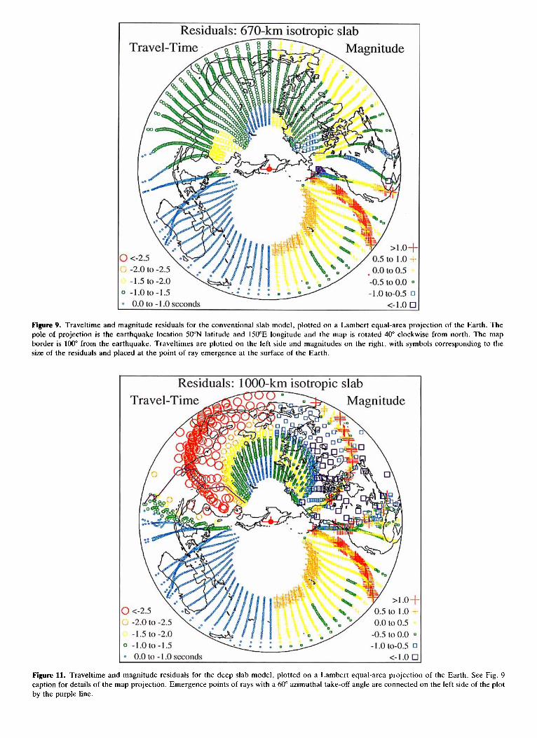
model are plotted on a Lambert equal-area projection with the pole of the projection centred on the Earthquake. The perimeter of the map is 100" from the pole of projection and the map is rotated 40" around the pole in a clockwise direction. Consequently, the strike direction is left to right across the page as indicated by the strike-dip symbol at the source (e.g. Fig. 9). The traveltime residuals can be plotted on the left side of the map and the magnitude residuals on the right because of the symmetry of the model. The residual symbols indicate where rays come to the surface after turning in the lower mantle and their alignments show paths of constant azimuthal take-off angle. The size of each symbol is proportional to the corresponding residual.

In the past, subduction-zone modelling has been primarily in 2-D (e.g. Weber 1990). To facilitate comparisons with these previous studies, the residuals for rays that have left the source in the plane perpendicular-strike are plotted in Figs 6a and 6b (traveltime residuals) and in Figs 7a and 7b (magnitude residuals).

The next sections describe the wavefront results for each model. Due to space and time restrictions, only lower-mantle P-waves have been considered. The results indicate that a study of core-phase effects will be very interesting. Other possibilities for future modelling are upper-mantle phases and S-waves.

4.1 Isotropic slab to 670 km

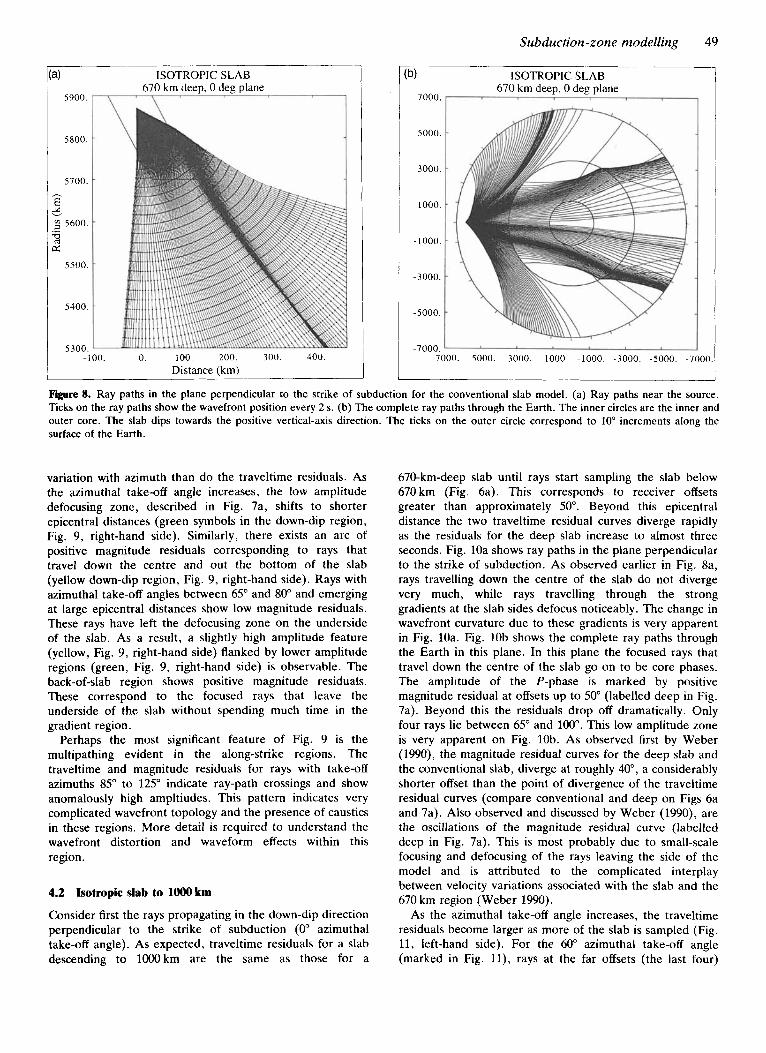
Even though the source is near the bottom of the slab in this model, significant variations in traveltimes and amplitudes, with respect to PREM, are observable. Fig. 6a shows traveltime residuals (those labelled conventional) ranging from 0.8 to 1.1 seconds for rays travelling in the down-dip direction perpendicular to the strike of the subduction zone. Rays with offsets less than 70" have left the slab from the upper edge. The rays beyond the 70" offset have left the slab

from the bottom. Fig. 8a shows the ray paths in the vicinity of the slab. The high-velocity slab region acts as an anti-waveguide by spraying rays out of the sides. The velocity contours of this model (Fig. 3) show that there are strong velocity gradients at the slab boundaries. Rays that travel through these gradient regions for some distance diverge considerably faster than those that travel down the centre of the slab or those that quickly leave the slab sides. In other words, the more time rays stay ,in the gradient regions the more they diverge (observable in Fig. 8a). This defocusing and focusing of energy is very apparent on the complete ray path plot (Fig. 8b). Fig. 7a (points labelled conventional) shows how the teleseismic amplitudes are sensitive to this. Low magnitude residuals are apparent at distances between 40" and 80". Up to 40" and beyond 80" the residuals are slightly positive as expected. Preliminary results suggest that variations in the nature of the slab-boundary velocity gradients can have significant effects on the wavefront (see discussion in section 5.2). The character of the traveltime and magnitude residuals for this model are very similar to those obtained by Weber (1990) for a similar slab model, although the size of his residuals is much larger because the source is at a depth of 130 km and situated closer to the upper edge of the slab. Weber (1990) has explored the traveltime and amplitude sensitivity to source depth for the 2-D case. To do so for the 3-D case would not be practical here. However, preliminary results certainly show that the wavefront effects due to the slab are exaggerated by shallower source depths (see conclusion).

As the azimuthal take-off angle increases the traveltime residuals generally become larger in absolute value (Fig. 9, left-hand side). This is simply because more of the slab is sampled. Traveltime residuals that lie in the back-of-slab (oceanic) region are small (approximately 0.5 s), increasing slightly for azimuths closer to the strike of subduction. The magnitude residuals (Fig. 9, right-hand side) show more

1 -1.0 to-1.5 I 0.0 to -1 .O seconds

1.0 to-0.5 0

<-1.0 13

Figure 9. Traveltime and magnitude residuals for the conventional slab model, plotted on a Lambert equal-area projection of the Earth. The pole of projection is the earthquake location 50"N latitude and 150"E longitude and the map i s rotated 40" clockwise from north. The map border is loo" from the earthquake. Traveltimes are plotted on the left side and magnitudes on the right, with symbols corresponding to the size of the residuals and placed at the point of ray emergence at the surface of the Earth.

Residuals: 1000-krn isotrotic slab

3 -1.010 -1.5 -1.0 to-0.5 0 2 0.0 to - 1 .O seconds <-1.0 c

Figure 11. Traveltime and magnitude residuals for the deep slab model, plotted on a Lambert equal-area projection of the Earth. See Fig. 9 caption for details of the map projection. Emergence points of rays with a HIo azimuthal take-off angle are connected on the left side of the plot by the purple line.

Residuals: sums-slab anisotrotw

-1.0 to -1.5 0.0 to - 1 .O seconds

.1.O to-0.5 0

<-1.0 0

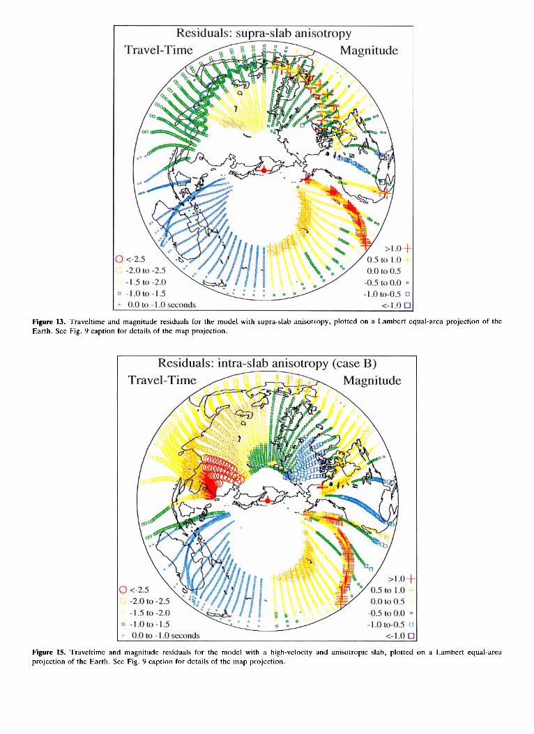
Figure W. Traveltime and magnitude residuals for the model with supra-slab anisotropy, plotted on a Lambert equal-area projection of the Earth. See Fig. 9 caption for details of the map projection.

Residuals: intra-slab anisotropy (case B)

0 -1.Oto-1.5 -1.0 to-0.5 0

<-1.0 c 0.0 to -1 .O seconds

Figure 15. Traveltime and magnitude residuals for the model with a high-velocity and anisotropic slab, plotted on a Lambert equal-area projection of the Earth. See Fig. 9 caption for details of the map projection.

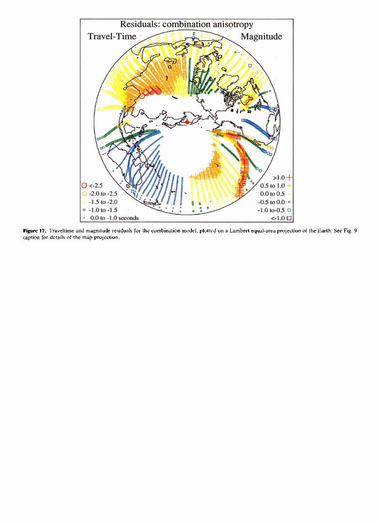
Residuals: combination anisotroDv

J -1.otO-1.5 n 0.0 to - 1 .O seconds

-1.0 to-0.5 0

<-I .o c Figure 17. Traveltime and magnitude residuals for the combination model, plotted on a Lambert equal-area projection of the Earth. See Fig. 9 caption for details of the map projection.

Subduction-zone modelling 49

:a) ISOTROPIC SLAB 670 krn deep. 0 deg plane

5900. r , I

5800.

5700.

.-

a: 5500.

5400.

Tznn. -100. 0. 100. 200. 300. 400.

Distance (km)

7000.

5000.

3000.

1000.

- 1000.

-3000.

-5000.

-7001)

ISOTROPIC SLAB 670 krn deep, 0 dee Dlane

.. 7000. 5000. 3000. 1000. -1000. -3000. -5000. -7000

Figure 8. Ray paths in the plane perpendicular to the strike of subduction for the conventional slab model. (a) Ray paths near the source. Ticks on the ray paths show the wavefront position every 2 s. (b) The complete ray paths through the Earth. The inner circles are the inner and outer core. The slab dips towards the positive vertical-axis direction. The ticks on the outer circle correspond to 10" increments along the surface of the Earth.

variation with azimuth than do the traveltime residuals. As the azimuthal take-off angle increases, the low amplitude defocusing zone, described in Fig. 7a, shifts to shorter epicentral distances (green symbols in the down-dip region, Fig. 9, right-hand side). Similarly, there exists an arc of positive magnitude residuals corresponding to rays that travel down the centre and out the bottom of the slab (yellow down-dip region, Fig. 9, right-hand side). Rays with azimuthal take-off angles between 65" and 80" and emerging at large epicentral distances show low magnitude residuals. These rays have left the defocusing zone on the underside of the slab. As a result, a slightly high amplitude feature (yellow, Fig. 9, right-hand side) flanked by lower amplitude regions (green, Fig. 9, right-hand side) is observable. The back-of-slab region shows positive magnitude residuals. These correspond to the focused rays that leave the underside of the slab without spending much time in the gradient region.

Perhaps the most significant feature of Fig. 9 is the multipathing evident in the along-strike regions. The traveltime and magnitude residuals for rays with take-off azimuths 85" to 125" indicate ray-path crossings and show anomalously high ampltiudes. This pattern indicates very complicated wavefront topology and the presence of caustics in these regions. More detail is required to understand the wavefront distortion and waveform effects within this region.

4.2 Isotropic slab to loo0 km

Consider first the rays propagating in the down-dip direction perpendicular to the strike of subduction (0' azimuthal take-off angle). As expected, traveltime residuals for a slab descending to 1OOOkm are the same as those for a

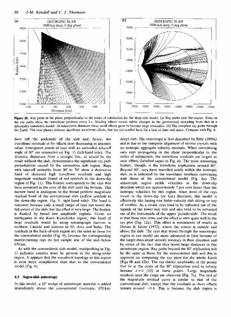
670-km-deep slab until rays start sampling the slab below 670km (Fig. 6a). This corresponds to receiver offsets greater than approximately SO". Beyond this epicentral distance the two traveltime residual curves diverge rapidly as the residuals for the deep slab increase to almost three seconds. Fig. 10a shows ray paths in the plane perpendicular to the strike of subduction. As observed earlier in Fig. 8a, rays travelling down the centre of the slab do not diverge very much, while rays travelling through the strong gradients at the slab sides defocus noticeably. The change in wavefront curvature due to these gradients is very apparent in Fig. 10a. Fig. 10b shows the complete ray paths through the Earth in this plane. In this plane the focused rays that travel down the centre of the slab go on to be core phases. The amplitude of the P-phase is marked by positive magnitude residual at offsets up to 50" (labelled deep in Fig. 7a). Beyond this the residuals drop off dramatically. Only four rays lie between 65" and 100". This low amplitude zone is very apparent on Fig. lob. As observed first by Weber (1990), the magnitude residual curves for the deep slab and the conventional slab, diverge at roughly W , a considerably shorter offset than the point of divergence of the traveltime residual curves (compare conventional and deep on Figs 6a and 7a). Also observed and discussed by Weber (1990), are the oscillations of the magnitude residual curve (labelled deep in Fig. 7a). This is most probably due to small-scale focusing and defocusing of the rays leaving the side of the model and is attributed to the complicated interplay between velocity variations associated with the slab and the 670 km region (Weber 1990).

As the azimuthal take-off angle increases, the traveltime residuals become larger as more of the slab is sampled (Fig. 11, left-hand side). For the 60" azimuthal take-off angle (marked in Fig. l l ) , rays at the far offsets (the last four)

50 J-M. Kendall and C. J . Thomson

a)

5900.

5800.

5700. h

E 5. 9 5600. .-

5500.

5400.

s300.

ISOTROPIC SLAB 1000 km deep, 0 deg plane

\ , \ ' I

- 100. 0. 100. 200. 300. 400 Distance (km)

:?4 7000.

5000.

3000.

1000.

- 1000.

-3000.

-5000.

-7000.

ISOTROPIC SLAB 1000 km deep, 0 deg plane

7000. 5000. 3000. 1000. -1000. -3000. -5000. -7000

Figure 10. Ray paths in the plane perpendicular to the strike of subduction for the deep slab model. (a) Ray paths near the source. Ticks on the ray paths show the wavefront position every 2s. Shading effects reveal subtle changes in the geometrical spreading from that in a spherically symmetric model. At teleseismic distances these small effects grow to become large anomalies. (b) The complete ray paths through the Earth. The core phases indicate significant wavefront effects, but are not studied here for a lack of time and space. Compare with Fig. 8.

have left the underside of the slab and, hence, the traveltime residuals at far offsets start decreasing in absolute value. Emergence points of rays with an azimuthal take-off angle of 60" are connected on Fig. 11 (left-hand side). The dramatic departure from a straight line, as would be the result without the slab, demonstrates the significant ray path perturbations caused by the anomalous slab region. Rays with take-off azimuths from 30" to 70" show a distinctive band of clustered high traveltime residuals and high magnitude residuals (band of red symbols in the down-dip region of Fig. 11). This feature corresponds to the rays that have remained in the core of the slab until the bottom. This narrow band is analogous to the broad positive magnitude residual band of the conventional slab (yellow symbols in the down-dip region, Fig. 9, right-hand side). The band is narrower because only a small range of rays can travel the full extent of the slab, but the effect is very large. The feature is flanked by broad low amplitude regions. Given an earthquake in the Kuril-Kamchatka region, this band of large residuals would lie along seismograph stations in northern Canada and stations in SE Asia and India. The residuals in the back-of-slab region are the same as those for the conventional model (Fig. 9), because the corresponding mantle-turning rays do not sample any of the slab below 670 km.

As with the conventional slab model, multipathing in Fig. 11 indicates caustics must be present in the along-strike region. It appears that the wavefront topology in this region is even more complicated than that in the conventional model (Fig. 9).

4.3 Supra-slab anisotropy

In this model, a 10" wedge of anisotropic material is added immediately above the conventional (isotropic, 670 km-

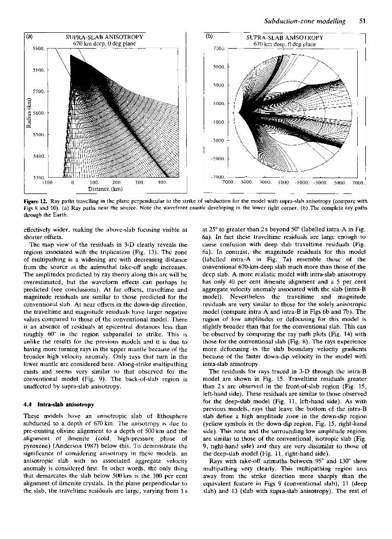
deep) slab. The anisotropy is that described by Ribe (1989a) and is due to the complete alignment of olivine crystals with no isotropic aggregate velocity anomaly. When considering only rays propagating in the plane perpendicular to the strike of subduction, the traveltime residuals are largest at near offsets (labelled supra in Fig. 6). The most interesting feature, though, is the traveltime triplication around 80". Beyond 80", rays have travelled solely within the isotropic slab, as is indicated by the traveltime residuals converging with those of the conventional model (Fig. 6a). The anisotropic region yields velocities in the down-dip direction which are approximately 7 per cent faster than the isotropic velocities for this region. Since most of the rays travel in the down-dip (or fast) direction, this model is effectively like having one faster-velocity slab sitting on top of another. As a result, rays tend to be refracted out of the topside of the lower real slab and also tend to be refracted out of the bottomside of the upper 'pseudo-slab'. The result is that these rays cross and the effect is seen quite well in the ray plot (Fig. 12a). This effect is reminiscent of results in Davies & Julian (1972), where the source is outside and above the slab. The rays that travel through the anisotropic region in our model are more advanced in time because of the larger-than-usual velocity anomaly in their direction and by virtue of the fact that they travel large distances in this anisotropic region. Ray paths beyond the 80" triplication will be the same as those for the conventional slab and this is apparent on comparing the ray plots for the whole Earth (Figs 8b and 12b). The ray theory amplitudes at the points that lie at the cusps of the 80" triplication tend to infinity because J = O (10) at these points. Large magnitude residuals near the cusps are observed (Fig. 7a). The rest of the magnitude residual curve is similar to that of the conventional slab, except that the residuals at short offsets remain around -0.4. This is because the slab region is

Subduction-zone modelling 51

SUPRA-SLAB ANISOTROPY a)

5900.

5800.

5700.

2 5

5600.

5500.

5400.

670 km deep, 0 deg plane \ . \ '

5300. -100. 0. 100. 200. 300. 400.

Distance (km)

.b) SUPRA-SLAB ANISOTROPY 670 km deep, 0 deg plane

7000. 7

5000.

3000.

1000.

- 1000.

-3000.

-5000.

-7000. ' 7000. 5000. 3000. 1000. -1000. -3000. -5000. -7000

Figure 12. Ray paths travelling in the plane perpendicular to the strike of subduction for the model with supra-slab anisotropy (compare with Figs 8 and 10). (a) Ray paths near the source. Note the wavefront caustic developing in the lower right corner. (b) The complete ray paths through the Earth

effectively wider, making the above-slab focusing visible at shorter offsets.

The map view of the residuals in 3-D clearly reveals the regions associated with the triplication (Fig. 13). The zone of multipathing is a widening arc with decreasing distance from the source as the azimuthal take-off angle increases. The amplitudes predicted by ray theory along this arc will be overestimated, but the waveform effects can perhaps be predicted (see conclusions). At far offsets, traveltime and magnitude residuals are similar to those predicted for the conventional slab. At near offsets in the down-dip direction, the traveltime and magnitude residuals have larger negative values compared to those of the conventional model. There is an absence of residuals at epicentral distances less than roughly 60" in the region subparallel to strike. This is unlike the results for the previous models and it is due to having more turning rays in the upper mantle because of the broader high velocity anomaly. Only rays that turn in the lower mantle are considered here. Along-strike multipathing exists and seems very similar to that observed for the conventional model (Fig. 9). The back-of-slab region is unaffected by supra-slab anisotropy.

4.4 Intra-slab anisotropy

These models have an anisotropic slab of lithosphere subducted to a depth of 670 km. The anisotropy is due to pre-existing olivine alignment to a depth of 500 km and the alignment of ilmenite (cold, high-pressure phase of pyroxene) (Anderson 1987) below this. To demonstrate the significance of considering anisotropy in these models, an anisotropic slab with no associated aggregate velocity anomaly is considered first. In other words, the only thing that demarcates the slab below 500 km is the 100 per cent alignment of ilmenite crystals. In the plane perpendicular to the slab, the traveltime residuals are large, varying from 1 s

at 25" to greater than 2 s beyond 50" (labelled intra-A in Fig. 6a). In fact these traveltime residuals are large enough to cause confusion with deep slab traveltime residuals (Fig. 6a). In contrast, the magnitude residuals for this model (labelled intra-A in Fig. 7a) resemble those of the conventional 670-km-deep slab much more than those of the deep slab. A more realistic model with intra-slab anisotropy has only 40 per cent ilmenite alignment and a 5 per cent aggregate velocity anomaly associated with the slab (intra-B model). Nevertheless the traveltime and magnitude residuals are very similar to those for the solely anisotropic model (compare intra-A and intra-B in Figs 6b and 7b). The region of low amplitudes or defocusing for this model is slightly broader than that for the conventional slab. This can be observed by comparing the ray path plots (Fig. 14) with those for the conventional slab (Fig. 8). The rays experience more defocusing in the slab boundary velocity gradients because of the faster down-dip velocity in the model with intra-slab anisotropy.

The residuals for rays traced in 3-D through the intra-B model are shown in Fig. 15. Traveltime residuals greater than 2 s are observed in the front-of-slab region (Fig. 15, left-hand side). These residuals are similar to those observed for the deep-slab model (Fig. 11, left-hand side). As with previous models, rays that leave the bottom of the intra-B slab define a high amplitude zone in the down-dip region (yellow symbols in the down-dip region, Fig. 15, right-hand side). This zone and the surrounding low amplitude regions are similar to those of the conventional, isotropic slab (Fig. 9, right-hand side) and they are very dissimilar to those of the deep-slab model (Fig. 11, right-hand side).

Rays with take-off azimuths between 95" and 130" show multipathing very clearly. This multipathing region arcs away from the strike direction more sharply than the equivalent feature in Figs 9 (conventional slab), 11 (deep slab) and 13 (slab with supra-siab anisotropy). The rest of

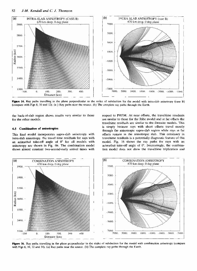
52 J-M. Kendall and C. J . Thomson

(4 5900.

5800.

5700. h

E e5 g 5600. .-

5500.

5400.

<?nn L

INTRA-SLAB ANISOTROPY (CASE B) 670 km deep, 0 den plane

__-I. -100. 0. 100. 200. 300. 400

Distance (km)

b) INTRA-SLAB ANISOTROPY (case B) 670 km deep, 0 deg plane

7000. ,

5000.

3000.

1000.

-1000.

-3000.

-5000.

-7000. ' I 7000. 5000. 3000. 1000. -1000. -3000. -5000. -7000

Figure 14. Ray paths travelling in the plane perpendicular to the strike of subduction for the model with intra-slab anisotropy (case B) (compare with Figs 8, 10 and 12). (a ) Ray paths near the source. (b) The complete ray paths through the Earth.

the back-of-slab region shows results very similar to those for the other models.

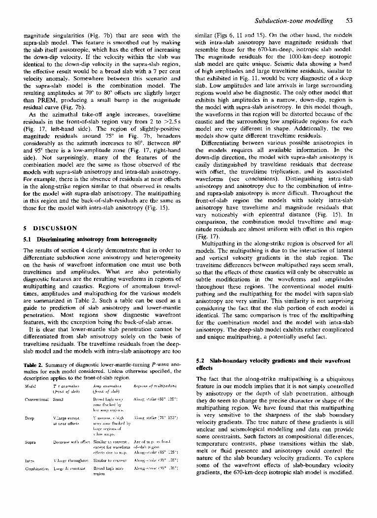
4.5 Combination of anisotropies

This final model incorporates supra-slab anisotropy with intra-slab anisotropy. the travel time residuals for rays with an azimuthal take-off angle of 0" for all models with anisotropy are shown in Fig. 6b. The combination model shows almost constant two-second-early arrival times with

COMBINATION ANISOTROPY 670 krn deep, 0 deg plane

I 5900.

5800.

5700. h

E c B 9 5600.

n: .-

5500.

5400.

0. 100. 200. 300. 400 5300. L

-100. Distance (km)

respect to PREM. At near offsets, the traveltime residuals are similar to those for the Ribe model and at far offsets the traveltime residuals are similar to the ilmenite models. This is simply because rays with short offsets travel mostly through the anisotropic supra-slab region while rays at far offsets remain in the anisotropic slab. This constancy in traveltime residuals is a potentially diagnostic feature of this model. Fig. 16 shows the ray paths for rays with an azimuthal take-off angle of 0". Interestingly, the combina- tion model does not show the traveltime triplication and

b) COMBINATION ANISOTROPY 670 km deep, 0 deg plane

I 7000.

5000.

3000.

1000.

-1000.

-3000.

-5000.

-7000. 7000. 9000. 3000. 1000. -1000 -3000. -5000 -7000

Figure 16. Ray paths travelling in the plane perpendicular to the strike of subduction for the model with combination anisotropy (compare with Figs 8, 10, 12 and 14). (a) Ray paths near the source. (b) The complete ray paths through the Earth.

Subduction-zone modelling 53

magnitude singularities (Fig. 7b) that are seen with the supra-slab model. This feature is smoothed out by making the slab itself anisotropic, which has the effect of increasing the down-dip velocity. If the velocity within the slab was identical to the down-dip velocity in the supra-slab region, the effective result would be a broad slab with a 7 per cent velocity anomaly. Somewhere between this scenario and the supra-slab model is the combination model. The resulting amplitudes at 70" to 80" offsets are slightly larger than PREM, producing a small bump in the magnitude residual curve (Fig. 7b).

As the azimuthal take-off angle increases, traveltime residuals in the front-of-slab region vary from 2 to >2Ss (Fig. 17, left-hand side). The region of slightly-positive magnitude residuals around 75" in Fig. 7b, broadens considerably as the azimuth increases to 80". Between 80" and 95" there is a low-amplitude zone (Fig. 17, right-hand side). Not surprisingly, many of the features of the combination model are the same as those observed of the models with supra-slab anisotropy and intra-slab anisotropy. For example, there is the absence of residuals at near offsets in the along-strike region similar to that observed in results for the model with supra-slab anisotropy. The multipathing in this region and the back-of-slab-residuals are the same as those for the model with intra-slab anisotropy (Fig. 15).

5 DISCUSSION

5.1 Discriminating anisotropy from heterogeneity

The results of section 4 clearly demonstrate that in order to differentiate subduction zone anisotropy and heterogeneity on the basis of wavefront information one must use both traveltimes and amplitudes. What are also potentially diagnostic features are the resulting waveforms in regions of multipathing and caustics. Regions of anomalous travel- times, amplitudes and multipathing for the various models are summarized in Table 2. Such a table can be used as a guide to prediction of slab anisotropy and lower-mantie penetration. Most regions show diagnostic wavefront features, with the exception being the back-of-slab areas.

It is clear that lower-mantle slab penetration cannot be differentiated from slab anisotropy solely on the basis of traveltime residuals. The traveltime residuals from the deep- slab model and the models with intra-slab anisotropy are too

Table 2. Summary of diagnostic lower-mantle-turning P-wave ano- malies for each model considered. Unless otherwise specified, the description applies to the front-of-slab region. Model T- i ammalie2 Amp anomalies Region3 of mulltpalhing

(f.ont of dab) (front of-.slab)

Conventional Small Broad high anip Along-btrikr (S9" 125") zone flankrd by low amp r+ona.

Deep V.large pxcupt V narrow. v.high Along-strikr (70" 125") a t m a r offsets amp zone flankcd by

1a rp rCgiollb of r . low a,n,,s.

rxrept for waveform of-4ali rrgion rffrcts due to n i . p

Supra Derrrasr with offset Snuilar to convent., Arc of 11r.p. 1x1 front

Akmg-strike (83" 123")

h t r a \'.large throiighout Siinilar t u coriwnt Aloiig->trik(, (05'-135")

Combination Large 9r conataxt Broad high nnlp Along-ctrlkr (93" 135") rrgi011

similar (Figs 6, 11 and 15). On the other hand, the models with intra-slab anisotropy have magnitude residuals that resemble those for the 670-km-deep, isotropic slab model. The magnitude residuals for the 1000-km-deep isotropic slab model are quite unique. Seismic data showing a band of high amplitudes and large traveltime residuals, similar to that exhibited in Fig. 11, would be very diagnostic of a deep slab. Low amplitudes and late arrivals in large surrounding regions would also be diagnostic. The only other model that exhibits high amplitudes in a narrow, down-dip, region is the model with supra-slab anisotropy. In this model though, the waveforms in this region will be distorted because of the caustic and the surrounding low amplitude regions for each model are very different in shape. Additionally, the two models show quite different traveltime residuals.

Differentiating between various possible anisotropies in the models requires all available information. In the down-dip direction, the model with supra-slab anisotropy is easily distinguished by traveltime residuals that decrease with offset, the traveltime triplication, and its associated waveforms (see conclusions). Distinguishing intra-slab anisotropy and anisotropy due to the combination of intra- and supra-slab anisotropy is more difficult. Throughout the front-of-slab region the models with solely intra-slab anisotropy have traveltime and magnitude residuals that vary noticeably with epicentral distance (Fig. 15). In comparison, the combination model traveltime and mag- nitude residuals are almost uniform with offset in this region (Fig. 17).

Multipathing in the along-strike region is observed for all models. The multipathing is due to the interaction of lateral and vertical velocity gradients in the slab region. The traveltime differences between multipathed rays seem small, so that the effects of these caustics will only be observable as subtle modifications in the waveforms and amplitudes throughout these regions. The conventional model multi- pathing and the multipathing for the model with supra-slab anisotropy are very similar. This similarity is not surprising considering the fact that the slab portion of each model is identical. The same comparison is true of the multipathing for the combination model and the model with intra-slab anisotropy. The deep-slab model exhibits rather complicated and unique multipathing, a potentially useful fact.

5.2 Slab-boundary velocity gradients and their wavefront effects

The fact that the along-strike multipathing is a ubiquitous feature in our models implies that it is not simply controlled by anisotropy or the depth of slab penetration, although they do seem to change the precise character or shape of the multipathing region. We have found that this multipathing is very sensitive to the sharpness of the slab boundary velocity gradients. The true nature of these gradients is still unclear and seismological modelling and data can provide some constraints. Such factors as compositional differences, temperature contrasts, phase transitions within the slab, melt or fluid presence and anisotropy could control the nature of the slab boundary velocity gradients. To explore some of the wavefront effects of slab-boundary velocity gradients, the 670-km-deep isotropic slab model is modified.

54 J-M. Kendall and C. J . Thomson

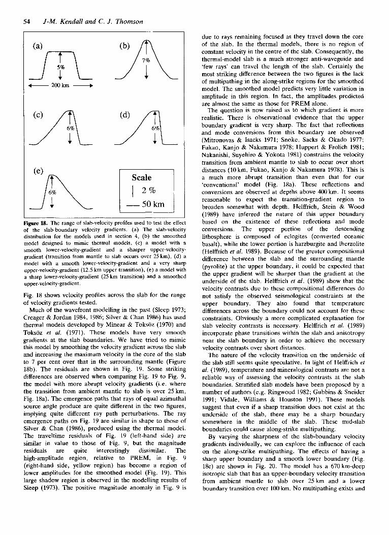
Figure 18. The range of slab-velocity profiles used to test the effect of the slab-boundary velocity gradients. (a) The slab-velocity distribution for the models used in section 4, (b) the smoothed model designed to mimic thermal models, (c) a model with a smooth lower-velocity-gradient and a sharper upper-velocity- gradient (transition from mantle to slab occurs over 25 km), (d) a model with a smooth lower-velocity-gradient and a very sharp upper-velocity-gradient (12.5 km upper transition), (e) a model with a sharp lower-velocity-gradient (25 km transition) and a smoothed upper-velocity-gradient .

Fig. 18 shows velocity profiles across the slab for the range of velocity gradients tested.

Much of the wavefront modelling in the past (Sleep 1973; Creager & Jordan 1984, 1986; Silver & Chan 1986) has used thermal models developed by Minear & Toksoz (1970) and Toksoz et al. (1971). These models have very smooth gradients at the slab boundaries. We have tried to mimic this model by smoothing the velocity gradient across the slab and increasing the maximum velocity in the core of the slab to 7 per cent over that in the surrounding mantle (Figure 18b). The residuals are shown in Fig. 19. Some striking differences are observed when comparing Fig. 19 to Fig. 9, the model with more abrupt velocity gradients (i.e. where the transition from ambient mantle to slab is over 25 km, Fig. Ma). The emergence paths that rays of equal azimuthal source angle produce are quite different in the two figures, implying quite different ray path perturbations. The ray emergence paths on Fig. 19 are similar in shape to those of Silver & Chan (1986), produced using the thermal model. The traveltime residuals of Fig. 19 (left-hand side) are similar in value to those of Fig. 9, but the magnitude residuals are quite interestingly dissimilar. The high-amplitude region, relative to PREM, in Fig. 9 (right-hand side, yellow region) has become a region of lower amplitudes for the smoothed model (Fig. 19). This large shadow region is observed in the modelling results of Sleep (1973). The positive magnitude anomaly in Fig. 9 is

due to rays remaining focused as they travel down the core of the slab. In the thermal models, there is no region of constant velocity in the centre of the slab. Consequently, the thermal-model slab is a much stronger anti-waveguide and ‘few rays’ can travel the length of the slab. Certainly the most striking difference between the two figures is the lack of multipathing in the along-strike regions for the smoothed model. The smoothed model predicts very little variation in amplitude in this region. In fact, the amplitudes predicted are almost the same as those for PREM alone.

The question is now raised as to which gradient is more realistic. There is observational evidence that the upper boundary gradient is very sharp. The fact that reflections and mode conversions from this boundary are observed (Mitronovas & Isacks 1971; Snoke, Sacks & Okado 1977; Fukao, Kanjo & Nakamura 1978; Huppert & Frolich 1981; Nakanishi, Suyehiro & Yokota 1981) constrains the velocity transition from ambient mantle to slab to occur over short distances (10 km, Fukao, Kanjo & Nakamura 1978). This is a much more abrupt transition than even that for our ‘conventional’ model (Fig. Ma). These reflections and conversions are observed at depths above 400 kin. It seems reasonable to expect the transition-gradient region to broaden somewhat with depth. Helffrich, Stein & Wood (1989) have inferred the nature of this upper boundary based on the existence of these reflections and mode conversions. The upper portion of the descending lithosphere is composed of eclogites (converted oceanic basalt), while the lower portion is harzburgite and lherzolite (Helffrich et af. 1989). Because of the greater compositional difference between the slab and the surrounding mantle (pyrolite) at the upper boundary, it could be expected that the upper gradient will be sharper than the gradient at the underside of the slab. Helffrich et al. (1989) show that the velocity contrasts due to these compositional differences do not satisfy the observed seismological constraints at the upper boundary. They also found that temperature differences across the boundary could not account for these constraints. Obviously a more complicated explanation for slab velocity contrasts is necessary. Helffrich et al. (1989) incorporate phase transitions within the slab and anisotropy near the slab boundary in order to achieve the necessary velocity contrasts over short distances.

The nature of the velocity transition on the underside of the slab still seems quite speculative. In light of Helffrich et al. (1989), temperature and mineralogical contrasts are not a reliable way of assessing the velocity contrasts at the slab boundaries. Stratified slab models have been proposed by a number of authors (e.g. Ringwood 1982; Gubbins & Sneider 1991; Vidale, Williams & Houston 1991). These models suggest that even if a sharp transition does not exist at the underside of the slab, there may be a sharp boundary somewhere in the middle of the slab. These mid-slab boundaries could cause along-strike multipathing.

By varying the sharpness of the slab-boundary velocity gradients individually, we can explore the influence of each on the along-strike multipathing. The effects of having a sharp upper boundary and a smooth lower boundary (Fig. 18c) are shown in Fig. 20. The model has a 670 km-deep isotropic slab that has an upper-boundary velocity transition from ambient mantle to slab over 25km and a lower boundary transition over 100 km. No multipathing exists and

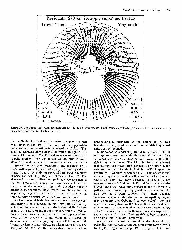
Subduction-zone modelling 55

Residuals: 670-km isotropic smoothed(b) slab

Figure 19. Traveltime and magnitude residuals for the model with smoothed slab-boundary velocity gradients and a maximum velocity anomaly of 7 per cent (profile b in Fig. 23)

the amplitudes in the down-dip region are quite different from those in Fig. 19. If the range of the upper-slab- boundary velocity transition is decreased to 12.5 km (Fig. 18d) the residuals shown in Fig. 21 result. In light of the results of Fukao el al. (1978) this does not seem too sharp a velocity gradient. For this model we do observe some along-strike multipathing. It is instructive to now reverse the nature of the two slab boundaries. The residuals for a model with a gradual (over 100 km) upper boundary velocity contrast and a more abrupt (over 25 km) lower boundary velocity contrast (Fig. 18e) are shown in Fig. 22. The along-strike region exhibits multipathing much like that in Fig. 9. These results imply that waveforms will be very sensitive to the nature of the slab boundary velocity gradients. Furthermore, these results have shown that the amplitudes, in general, are very sensitive to variations in these velocity gradients, while the traveltimes are not.

In all of our models the back-of-slab results are not very informative. This is because the rays leave the slab quickly and do not have time to be perturbed substantially. In light of this, the nature of the lower-boundary velocity gradient does not seem as important as that of the upper gradient. Most of our diagnostic results occur in the down-dip direction where the emerging rays have left the upper slab boundary where a sharp velocity transition seems likely. The exception to this is the along-strike region where

multipathing is diagnostic of the nature of the slab boundary velocity gradient as well as the slab length and anisotropy of the model.

In the smoothed model (Fig. 18b) it is, in a sense, difficult for rays to travel far within the core of the slab. The smoothed slab Acts as a stronger anti-waveguide than the slab in the initial models (Fig. 18a). Studies have indicated that the rays can travel large distances along strike in the core of the slab (Ansell & Gubbins 1986; Huppert & Frolich 1987; Gubbins & Snieder 1991). This observational evidence implies that models with a constant velocity region within the slab, like those discussed in section 4, are necessary. Ansell & Gubbins (1986) and Gubbins & Snieder (1991) found that waveforms corresponding to these ray paths are very high-frequency (5-10Hz). In a sense, the slab acts as a high-frequency filter. High-frequency waveform effects in the along-strike multipathing region may be observable. Gubbins & Snieder (1991) infer that rays travel along-strike in the Tonga-Kermadec slab in a reverberatory or modal fashion. A sharper slab-boundary velocity contrast than that in thermal models is required to support this explanation. Their modelling best supports a slab with a thin (6-15 km), uniform lid.

Another model constraint would be the observation of pulse distortion at receivers in the along-strike region. Work by Fujita, Rogers & Sleep (1980), Rogers (1982) and

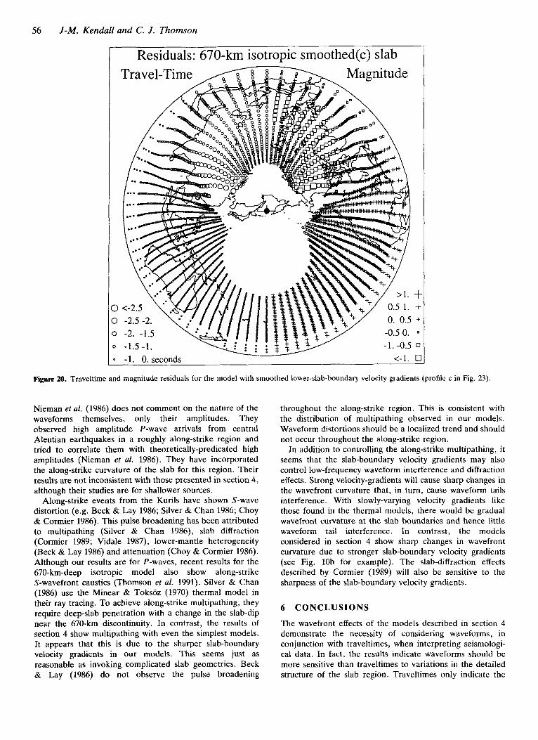
56 J-M. Kendall and C. J . Thomson

Residuals: 670-km isotropic smoothed(c) slab

Figure 20. Traveltime and magnitude residuals for the model with smoothed lower-stab-boundary velocity gradients (profile c in Fig. 23).

Nieman et af. (1986) does not comment on the nature of the waveforms themselves, only their amplitudes. They observed high amplitude P-wave arrivals from central Aleutian earthquakes in a roughly along-strike region and tried to correlate them with theoretically-predicated high amplitudes (Nieman et al. 1986). They have incorporated the along-strike curvature of the slab for this region. Their results are not inconsistent with those presented in section 4, although their studies are for shallower sources.

Along-strike events from the Kurils have shown S-wave distortion (e.g. Beck & Lay 1986; Silver & Chan 1986; Choy & Cormier 1986). This pulse broadening has been attributed to multipathing (Silver & Chan 1986), slab diffraction (Cormier 1989; Vidale 1987), lower-mantle heterogeneity (Beck & Lay 1986) and attenuation (Choy & Cormier 1986). Although our results are for P-waves, recent results for the 670-km-deep isotropic model also show along-strike S-wavefront caustics (Thomson et af. 1991). Silver & Chan (1986) use the Minear & Toksoz (1970) thermal model in their ray tracing. To achieve along-strike multipathing, they require deep-slab penetration with a change in the slab-dip near the 670-km discontinuity. In contrast, the results of section 4 show multipathing with even the simplest models. It appears that this is due to the sharper slab-boundary velocity gradients in our models. This seems just as reasonable as invoking complicated slab geometries. Beck & Lay (1986) do not observe the pulse broadening

throughout the along-strike region. This is consistent with the distribution of multipathing observed in our models. Waveform distortions should be a localized trend and should not occur throughout the along-strike region.

In addition to controlling the along-strike multipathing, it seems that the slab-boundary velocity gradients may also control low-frequency waveform interference and diffraction effects. Strong velocity-gradients will cause sharp changes in the wavefront curvature that, in turn, cause waveform tails interference. With slowly-varying velocity gradients like those found in the thermal models, there would be gradual wavefront curvature at the slab boundaries and hence little waveform tail interference. In contrast, the models considered in section 4 show sharp changes in wavefront curvature due to stronger slab-boundary velocity gradients (see Fig. 10b for example). The slab-diffraction effects described by Cormier (1989) will also be sensitive to the sharpness of the slab-boundary velocity gradients.

6 CONCLUSIONS

The wavefront effects of the models described in section 4 demonstrate the necessity of considering waveforms, in conjunction with traveltimes, when interpreting seismologi- cal data. In fact, the results indicate waveforms should be more sensitive than traveltimes to variations in the detailed structure of the slab region. Traveltimes only indicate the

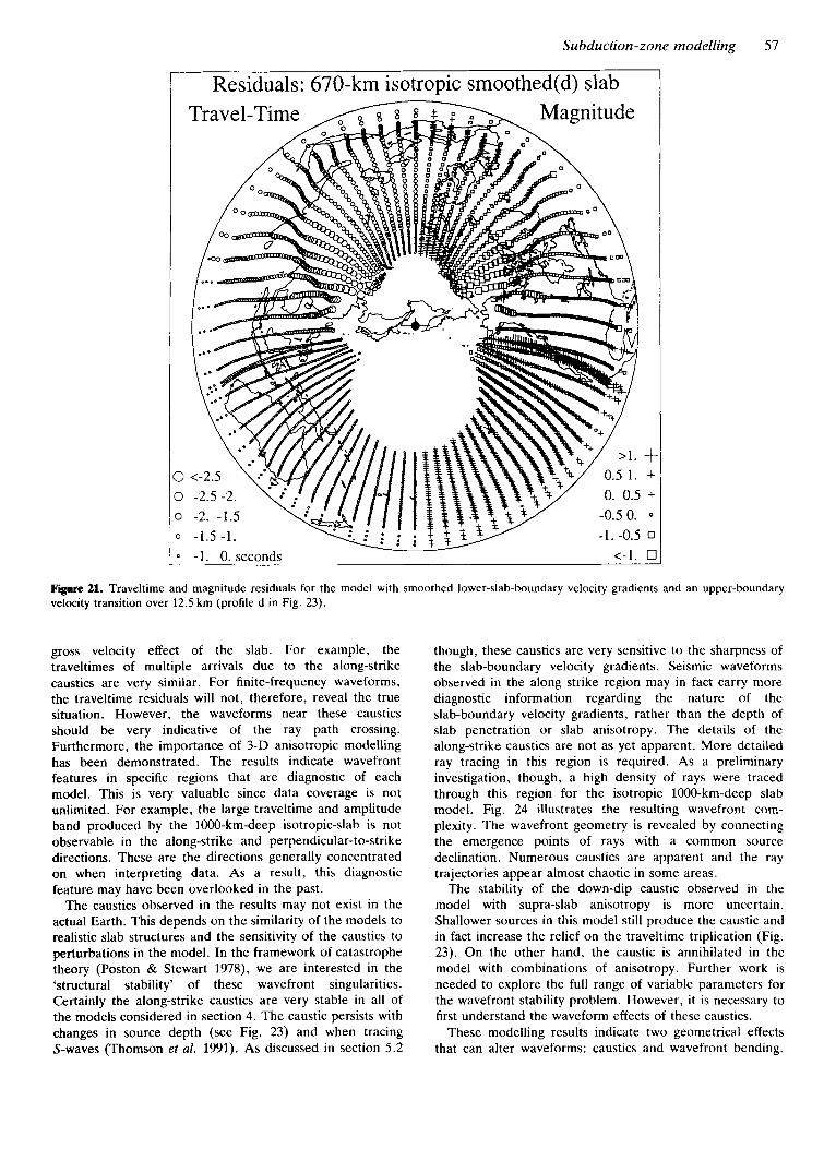
Subduction-zone modelling 57

Residuals: 670-km isotropic smoothed(d) slab

Figure 21. Traveltime and magnitude residuals for the model with smoothed lower-slab-boundary velocity gradients and an upper-boundary velocity transition over 12.5 km (profile d in Fig. 23).

gross velocity effect of the slab. For example, the traveltimes of multiple arrivals due to the along-strike caustics are very similar. For finite-frequency waveforms, the traveltime residuals will not, therefore, reveal the true situation. However, the waveforms near these caustics should be very indicative of the ray path crossing. Furthermore, the importance of 3-D anisotropic modelling has been demonstrated. The results indicate wavefront features in specific regions that are diagnostic of each model. This is very valuable since data coverage is not unlimited. For example, the large traveltime and amplitude band produced by the 1000-km-deep isotropic-slab is not observable in the along-strike and perpendicular-to-strike directions. These are the directions generally concentrated on when interpreting data. As a result, this diagnostic feature may have been overlooked in the past.

The caustics observed in the results may not exist in the actual Earth. This depends on the similarity of the models to realistic slab structures and the sensitivity of the caustics to perturbations in the model. In the framework of catastrophe theory (Poston & Stewart 1978), we are interested in the ‘structural stability’ of these wavefront singularities. Certainly the along-strike caustics are very stable in all of the models considered in section 4. The caustic persists with changes in source depth (see Fig. 23) and when tracing S-waves (Thomson et al. 1991). As discussed in section 5.2

though, these caustics are very sensitive to the sharpness of the slab-boundary velocity gradients. Seismic waveforms observed in the along strike region may in fact carry more diagnostic information regarding the nature of the slab-boundary velocity gradients, rather than the depth of slab penetration or slab anisotropy. The details of the along-strike caustics are not as yet apparent. More detailed ray tracing in this region is required. As a preliminary investigation, though, a high density of rays were traced through this region for the isotropic 1000-km-deep slab model. Fig. 24 illustrates the resulting wavefront com- plexity. The wavefront geometry is revealed by connecting the emergence points of rays with a common source declination. Numerous caustics are apparent and the ray trajectories appear almost chaotic in some areas.

The stability of the down-dip caustic observed in the model with supra-slab anisotropy is more uncertain. Shallower sources in this model still produce the caustic and in fact increase the relief on the traveltime triplication (Fig. 23). On the other hand, the caustic is annihilated in the model with combinations of anisotropy. Further work is needed to explore the full range of variable parameters for the wavefront stability problem. However, it is necessary to first understand the waveform effects of these caustics.

These modelling results indicate two geometrical effects that can alter waveforms: caustics and wavefront bending.

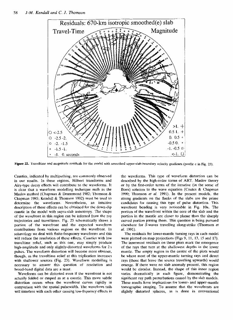
58 J - M . Kendall and C . J . Thomson

Residuals: 670-km isotropic smoothed(e) slab

<-1. c I -1. 0. seconds

Figure 22. Traveltime and magnitude residuals for the model with smoothed upper-slab-boundary velocity gradients (profile e in Fig. 23) .

Caustics, indicated by multipathing, are commonly observed in our results. In these regions, Hilbert transforms and Airy-type decay effects will contribute to the waveforms. It is clear that a waveform modelling technique such as the Maslov method (Chapman & Drummond 1982; Thomson & Chapman 1985; Kendall & Thomson 1992) must be used to determine the waveforms. Nevertheless, an intuitive description of these effects can be obtained for the down-dip caustic in the model with supra-slab anisotropy. The shape of the wavefront in this region can be inferred from the ray trajectories and traveltimes. Fig. 25 schematically shows a portion of the wavefront and the expected waveform contributions from various regions on the wavefront. In seismology we deal with finite-frequency waveforms and this will reduce the resolution of these effects. Caustics with low traveltime relief, such as this one, may simply produce high-amplitude and only slightly-distorted waveforms for 2 s pulses. The waveform distortion will become more obvious, though, as the traveltime relief at this triplication increases with shallower sources (Fig. 23). Waveform modelling is necessary to answer this question of resolution and broad-band digital data are a must.

Waveforms can be distorted even if the wavefront is not actually folded or cusped as at a caustic. This more subtle distortion occurs when the wavefront curves rapidly in comparison with the spatial pulsewidth. The waveform tails will interfere with each other causing low-frquency effects in

the waveforms. This type of waveform distortion can be described by the high-order terms of ART, Maslov theory or by the first-order terms of the iterative (in the sense of Born) solution to the wave equation (Coates & Chapman 1990; Thomson et af. 1991). In the present models, the strong gradients on the flanks of the slabs are the prime candidates for causing this type of pulse distortion. This wavefront bending is very noticeable in Fig. 10a. The portion of the wavefront within the core of the slab and the portion in the mantle are closer to planar than the sharply curved portion joining them. This question is being pursued elsewhere for S-waves travelling along-strike (Thomson et af. 1991).

The residuals for lower-mantle turning rays in each model were plotted on map projections (Figs 9, 11, 13, 15 and 17). The innermost residuals on these plots mark the emergence of the rays that turn at the shallowest depths in the lower mantle. The empty region in the centre of the plots would be where most of the upper-mantle turning rays and direct rays (those that leave the source travelling upwards) would emerge. If there were no slab anomaly present, this region would be circular. Instead, the shape of this inner region varies dramatically in each figure, demonstrating the significant ray path perturbations caused by the slab models. These results have implications for lower- and upper-mantle tomographic imaging. To assume that the wavefronts are slightly distorted spheres, as is done in conventional

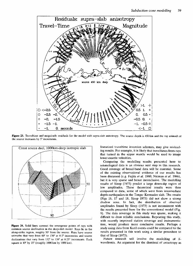
Subduction-zone modelling 59

Residuals: supra-slab anisotropy

Figure 23. Traveltime and magnitude residuals for the model with supra-slab anisotropy. The source depth is 450 km and the ray azimuth at the source increases by 5" increments.

Const source decl, 1000km-deep isotropic slab

50

Figure 24. Solid lines connect the emergence points of rays with common source declination in the deep-slab model. Rays lie in the along-strike region, roughly 50" from the source. Rays have source azimuths that vary from 60" to 130" at 0.5" increments and source declinations that vary from 132" to 139" at 0.25" increments. Each square is 10" by 10" (roughly loo0 km by loo0 km).

linearized traveltime inversion schemes, may give mislead- ing results. For example, it is likely that traveltimes from rays that turned in the upper mantle would be used to image lower-mantle velocities.

Comparing the modelling results presented here to seismological data is an obvious next step in this research. Good coverage of broad-band data will be essential. Some of the existing observational evidence of our results has been discussed (e.g. Fujita et af. 1980; Nieman et af. 1986), but it is very sparse and hence inconclusive. The modelling results of Sleep (1973) predict a large down-dip region of low amplitudes. These theoretical results were then compared to data, some of which were from intermediate depth earthquakes in the Tonga-Kermadec slab. The results (Figs 16, 17 and 18, Sleep 1973) did not show a strong shadow zone. In fact, the distribution of observed amplitudes found by Sleep (1973) is not inconsistent with the results presented here for the conventional model (Fig. 9). The data coverage in this study was sparse, making it difficult to draw reliable conclusions. Repeating this study, with recently improved station coverage and instrumenta- tion, would produce more conclusive results. Perhaps a study using data from Kuril events could be compared to the results presented in this work using a similar procedure to that of Sleep (1973).

Future research will involve the modelling of S- wavefronts. An argument for the dismissal of anisotropy as

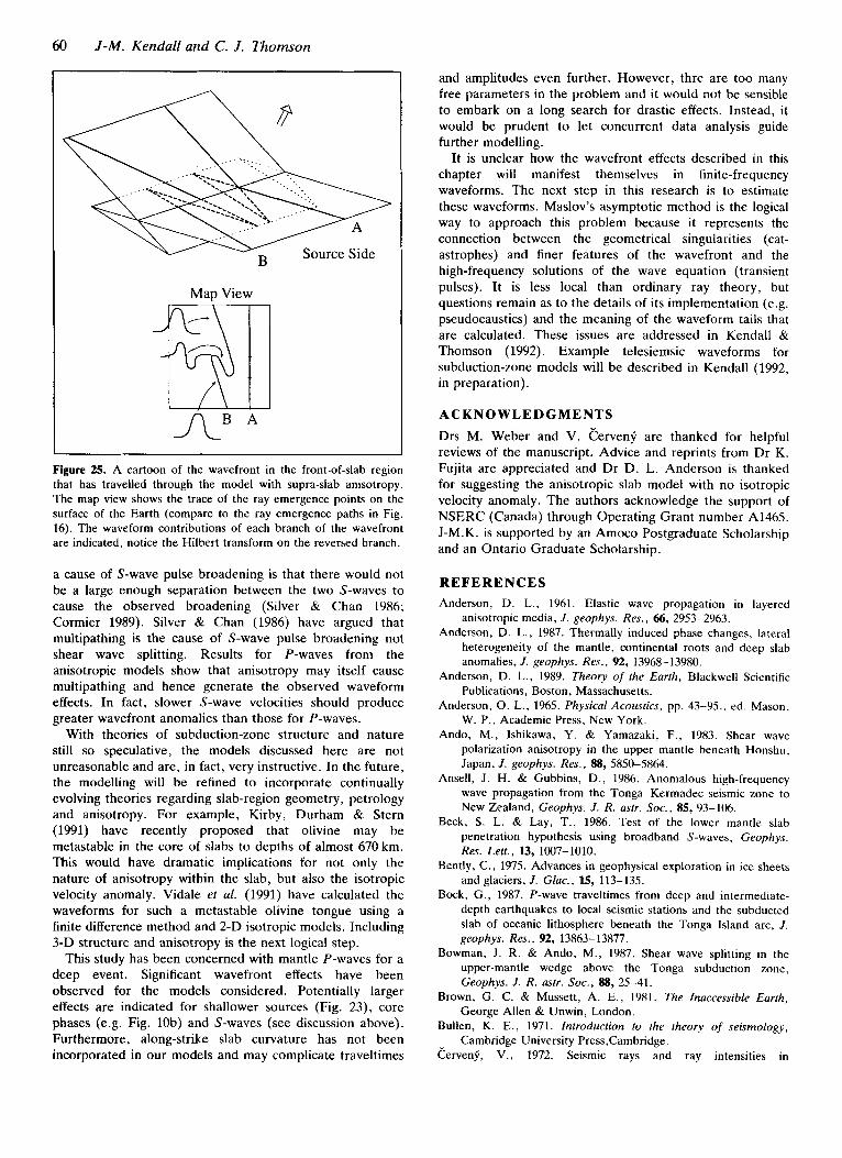
60 J - M . Kendall and C. J . Thomson

Map View m -AB A

Figure 25. A cartoon of the wavefront in the front-of-slab region that has travelled through the model with supra-slab anisotropy. The map view shows the trace of the ray emergence points on the surface of the Earth (compare to the ray emergence paths in Fig. 16). The waveform contributions of each branch of the wavefront are indicated, notice the Hilhert transform on the reversed branch.

a cause of S-wave pulse broadening is that there would not be a large enough separation between the two S-waves to cause the observed broadening (Silver & Chan 1986; Cormier 1989). Silver & Chan (1986) have argued that multipathing is the cause of S-wave pulse broadening not shear wave splitting. Results for P-waves from the anisotropic models show that anisotropy may itself cause multipathing and hence generate the observed waveform effects. In fact, slower S-wave velocities should produce greater wavefront anomalies than those for P-waves.

With theories of subduction-zone structure and nature still so speculative, the models discussed here are not unreasonable and are, in fact, very instructive. In the future, the modelling will be refined to incorporate continually evolving theories regarding slab-region geometry, petrology and anisotropy. For example, Kirby, Durham & Stern (199 1) have recently proposed that olivine may be metastable in the core of slabs to depths of almost 670 km. This would have dramatic implications for not only the nature of anisotropy within the slab, but also the isotropic velocity anomaly. Vidale et al. (1991) have calculated the waveforms for such a metastable olivine tongue using a finite difference method and 2-D isotropic models. Including 3-D structure and anisotropy is the next logical step.

This study has been concerned with mantle P-waves for a deep event. Significant wavefront effects have been observed for the models considered. Potentially larger effects are indicated for shallower sources (Fig. 23), core phases (e.g. Fig. lob) and S-waves (see discussion above). Furthermore, along-strike slab curvature has not been incorporated in our models and may complicate traveltimes

and amplitudes even further. However, thre are too many free parameters in the problem and it would not be sensible to embark on a long search for drastic effects. Instead, it would be prudent to let concurrent data analysis guide further modelling.

It is unclear how the wavefront effects described in this chapter will manifest themselves in finite-frequency waveforms. The next step in this research is to estimate these waveforms. Maslov’s asymptotic method is the logical way to approach this problem because it represents the connection between the geometrical singularities (cat- astrophes) and finer features of the wavefront and the high-frequency solutions of the wave equation (transient pulses). It is less local than ordinary ray theory, but questions remain as to the details of its implementation (e.g. pseudocaustics) and the meaning of the waveform tails that are calculated. These issues are addressed in Kendall & Thomson (1992). Example telesiemsic waveforms for subduction-zone models will be described in Kendall (1992, in preparation).

ACKNOWLEDGMENTS Drs M. Weber and V. Cervenq are thanked for helpful reviews of the manuscript. Advice and reprints from D r K. Fujita are appreciated and Dr D. L. Anderson is thanked for suggesting the anisotropic slab model with no isotropic velocity anomaly. The authors acknowledge the support of NSERC (Canada) through Operating Grant number A1465. J-M.K. is supported by an Amoco Postgraduate Scholarship and an Ontario Graduate Scholarship.

REFERENCES Anderson, D. L., 1961. Elastic wave propagation in layered

anisotropic media, J. geophys. Res., 66, 2953-2963. Anderson, D. L., 1987. Thermally induced phase changes, lateral

heterogeneity of the mantle, continental roots and deep slab anomalies, J. geophys. Res., 92, 13968-13980.

Anderson, D. L., 1989. Theory of the Earth, Blackwell Scientific Publications, Boston, Massachusetts.

Anderson, 0. L., 1965. Physical Acoustics, pp. 43-95., ed. Mason, W. P., Academic Press, New York.

Ando, M., Ishikawa, Y. & Yamazaki, F., 1983. Shear wave polarization anisotropy in the upper mantle beneath Honshu, Japan, J. geophys. Res., 88, 5850-5864.

Ansell, J. H. & Gubbins, D., 1986. Anomalous high-frequency wave propagation from the Tonga-Kermadec seismic zone to New Zealand, Geophys. J. R. astr. SOC., 85, 93-106.

Beck, S. L. & Lay, T., 1986. Test of the lower mantle slab penetration hypothesis using broadband S-waves, Geophys. Res. Lett., 13, 1007-1010.

Bently, C., 1975. Advances in geophysical exploration in Ice sheets and glaciers, J. Glac., 15, 113-135.

Bock, G., 1987. P-wave traveltimes from deep and intermediate- depth earthquakes to local seismic stations and the subducted slab of oceanic lithosphere beneath the Tonga Island arc, J. geophys. Res., 92, 13863-13877.

Bowman, J. R. & Ando, M., 1987. Shear wave splitting in the upper-mantle wedge above the Tonga subduction zone, Geophys. J. R. astr. SOC., 88, 25-41.

Brown, G. C. & Mussett, A. E., 1981. The Inaccessible Earth, George Allen & Unwin, London.

Bullen, K. E., 1971. lnfroduction to the theory of seismology, Cambridge University Press,Cambridge.

EervenL, V., 1972. Seismic rays and ray intensities in

Subduction-zone modelling 61

inhomogeneous anisotropic media, Geophys. J . R. astr. Soc., 29, 1-13.

Cervenq, V. & Ravindra, R., 1971, Theory of seismic head waves, University of Toronto Press, Toronto.

Cerveng, V., Popov, M. M., PSenEik, I., 1982. Computation of wavefields in inhomogeneous med iaaauss i an beam ap- proach, Geophys. J . R. astr. Soc., 70, 109-128.

Chapman, C. H. & Drummond, R., 1982. Body-wave seismograms in inhomogeneous media using Maslov asymptotic theory, Bull. seism. Soc. Am, 72, S277-S317.

Choy, G. L., & Cormier, V. F., 1986. Direct measurement of the mantle attenuation operator from broadband P - and S-waveforms, 1. geophys. Rex, 91, 7326-7342.

Christensen, N. I. & Lindquist, V. F., 1982. Pyroxene orientation within the upper mantle, Bull. Geol. Soc. A m . , 93, 279-288.

Cleary, J., 1967. Azimuthal variations of the longshot source term, Earth planet. Sci. Lett., 3, 29-37.

Coates, R. T. & Chapman, C. H., 1990. Quasi-shear wave coupling in weakly anisotropic 3-D media, Geophys. J . Int., 103,

Cormier, V. F., 1989. Slab diffraction of S-waves, J . geophys. Res.,

Cormier, V. F., 1990. Slab diffraction and its physical origins: predictions from a generalized Born Approximation, EOS Trans. Am. geophys. Un., 71, 1461.

Courant, R. & Hilbert, D., 1962. Methods of Mathematical Physics, Interscience Publishers, John Wiley & Sons, New York.

Creager, K. C. & Joidan, T. H., 1984. Slab penetration into the lower mantle, J . geophys. Res., 89, 3031-3049.

Creager, K. C. & Jordan, T. H., 1986. Slab penetration into the lower mantle beneath the Mariana and other island arcs of the northwest Pacific, J . geophys. Res., 91, 3573-3589.

Davies, D. & Julian, B. R. , 1972. A study of short period P-wave signals from Longshot, Geophys. J . R. astr. Soc., 29, 185-202.

Davis, H. F. & Snider, A. D., 1979. Introduction to Vector Analysis, 4th edn, Allyn and Bacon, Boston, Massachusetts.

Dziewonski, A. M., & Anderson, D. L., 1981. Preliminary reference earth model, Phys. Earth planet. Int. , 25, 297-356.

Engdahl, E. R., Vidale, J . E. & Cormier, V. F., 1989. Wave propagation in subducted lithospheric slabs, in Digital seismology and fine modelling of the lithosphere, eds Cassinis, R., Nolet, G . & Panza, G . F., Plenum Press, New York.

Fischer, K. M., Jordan, T. H. & Creager, K. C., 1988. Seismic constraints on the morphology of deep slabs, J . geophys. Res.,

Fujita, K., Rogers, W. J. Jr. & Sleep, N. H., 1980. Enhanced arrivals due to subducting slabs, EOS Trans. Am. geophys. Un., 61, 1045.

Fujita, K., Engdahl, E. R. & Sleep, N . H . , 1981. Subduction zone calibration and teleseismic relocation of thrust zone events in the central Aleutian Islands, Bull. seism. Soc. A m . , 71,

Fukao, Y., 1984. Evidence from core-reflected shear waves for anisotropy in the Earth’s mantle. Nature, 309, 694-698.

Fukao, Y., Kanjo, K. & Nakamura, I . , 1978. Deep seismic zone as an upper mantle reflector of body waves, Nature, 272,606-608.

Fukao, Y., Obayashi, M. & Inoue, H . , 1992. Subducting slabs stagnant in the mantle transition zone, J . geophys. Res., 97,

Gubbins, D. & Snieder, R., 1991. Dispersion of P-waves in subducted lithosphere: evidence for an eclogite layer, J . geophys. Res., 96, 6321-6333.

Guest, W. S., Spencer, C. P. & Thomson, C . J . , 1992. Anisotropic R /T calculations and ray tracing with application to a crustal survey from the East Greenland Shelf, Geophys. J . Int., submitted.

Hearmon, R. F. S . , 1961. Introduction to applied anisotropic elasticity, Clarenden Press, Oxford.

30 1-320.

94, 3006-3024.

93, 4773-4783.

1805- 1828.

4809-4822.

Helbig, K., 1966. A graphical method for the construction of rays and travel times in spherically layered media, 11, Bull. seism. SOC. Am. , 56, 527-559.

Helffrich, G. R., Stein, S. & Wood, B. J., 1989. Subduction zone thermal structure and mineralogy and their relationship to seismic wave reflections and conversions at the slab/mantle interface, J . geophys. Res., 94, 753-763.

Hill, R., 1952. The elastic behaviour of a crystalline aggregate, Proc. phys. Soc. Lond. A, 65, 349-354.

Huppert, L. N. & Frolich, C., 1981. The P-velocity within the Tonga Benioff zone determined from traced rays and observations, J . geophys. Res., 86, 3771-3782.

Jacob, K. H. , 1970. Three-dimensional seismic ray tracing in a laterally heterogeneous spherical Earth, J . geophys. Res., 75,

Jordan, T. H., 1977. Lithospheric slab penetration into the lower mantle beneath the sea of Okhotsk, J . Geophys., 43, 473-496.

Julian, B. R., 1970. Ray tracing in arbitrarily heterogeneous media, Technical note 1970-45, Lincoln Laboratory, Massachusetts Institute of Technology, Lexington, Massachusetts.

Julian, B. R. & Gubbins, D., 1977. Three-dimensional seismic ray tracing, J . Geophys., 43, 95-113.

Kendall, J-M., 1991. Contributions to the theory and modelling of seismic waves in anisotropic inhomogeneous media with applications to subduction zones, Ph. D. thesis, Queen’ University, Kingston, Ontario.

Kendall, J-M. & Thomson, C. J . , 1989. A comment on the form of the geometrical spreading equations, with some examples of seismic ray tracing in inhomogeneous, anisotropic media, Geophys. J . Int., 99, 401-413.

Kendall, J-M. & Thomson, C. J . , 1992. Maslov ray summation, pseudocaustics, causality, Lagrangian equivalence and transient seismic waveforms, Geophys. J . lnt., in press.

Kendall, J-M., Guest, W. S. 8r Thomson, C. J. , 1992. Ray-theory Green’s function reciprocity and ray-centered coordinates in anisotropic media, Geophys. J . Int . , 108, 364-371.

Kirby, S. H., Durham, W. B. & Stern, L. A. , 1991. Mantle phase changes and deep-earthquake faulting in subducting litho- sphere, Science, 252, 216-225.

Kumazawa, M. & Anderson, 0. L., 1969. Elastic moduli, pressure derivatives and temperature derivatives of a single-crystal olivine and a single crystal forsterite, 1. geophys. Res., 74,

Madariaga, R. , & Papadimitriou, P., 1985. Gaussian beam modelling of upper mantle phases, Ann. Geophys., 6, 799-812.

McKenzie, D. P., 1979. Finite deformation during fluid flow, Geophys. J . R. astr. Soc., 58, 689-715.

Mathews, J. & Walker, R. L., 1970. Mathematical methods of physics, W. A. Benjamin, Menlo Park, California.

Minear, J . W. & Toksoz, M. N . , 1970. Thermal regime of a downgoing slab and new global tectonics, J . geophys. Res., 75,

Mitronovas, W. & B. L. Isacks, 1971. Seismic velocity anomalies in the upper mantle beneath the Tonga-Kermadec Island arc, J . geophys. Res., 76, 7154-7180.

Murry, D. A, , 1916. Sphericaf trigonometry, Longmans, Green & Co., London.

Musgrave, M. J. P., 1985. Acoustic axes in orthorhombic media, Proc. phys. SOC. Lond. A , 401, 131-143.

Nakanishi, I. & Suyehiro, K. & Yokota, T., 1981. Regional variations of amplitudes of ScSp phases observed in the Japanese Islands, Geophys. J . R. astr. Soc., 67, 615-634.

Nieman, T. L., Fujita, K. & Rogers, W. J. Jr., 1986. Teleseismic mislocation of earthquakes in island arcs-theoretical results, J . Phys. Earth, 34, 43-70.

Nowack, R., & Aki, K., 1984. The two-dimensional Gaussian beam synthetic method: testing and application, J . geophys. Res.,

6675-6689.

596 1 -5972.

1397-1419.

89, 7797-7819.

62 J - M . Kendall and C. J . Thomson

Popov, M. M., 1982. A new method of computation of wave fields using Gaussian beams, Waue Motion, 4, 85-97.

Poston, T. & Stewart, I. N., 1978. Catastrophe theory and its application, Pitman, London.

Reuss. A , , 1929. Berechnung der Fliessgrenze von Mischkristallen auf Grund der Plastitatsbedingung fur Einkristalle, Z. Angew. Math. Mech, 9, 49-58.

Ribe, N. M., 1989a. Seismic anisotropy and mantle flow, J. geophys. Res., 94, 4213-4223.

Ribe, N. M., 1989b. A continuum theory for lattice preferred orientation, Geophys. J. R. astr. SOC., 97, 199-207.

Ringwood, 1982. Phase transformations and differentiation in subducted lithosphere: implications for mantle dynamics, basalt petrogenesis, and crustal evolution, J. Geol., 90, 611-643.

Rogers, W. J . Jr., 1982. The effects of subducting slabs on seismic amplitudes and traveltimes from forearc and outer rise earthquakes, M.Sc. Thesis, Michigan State University, Michigan.

Silver, P. G. & Chan, W. W., 1986. Observations of body wave multipathing from broad-band seismigrams: evidence for lower mantle slab penetration beneath the sea of Okhotsk, J. geophys. Res., 91, 13787-13802.

Silver, P. G., Carlson, R. W. & Olson, P., 1989. Deep slabs, geochemical heterogeneity, and the large-scale structure of mantle convection: investigation of an enduring paradox, Ann. Rev. Earth planet. Sci., 16, 477-541.

Sleep, N. H., 1973. Teleseismic P-wave transmission through slabs, Bull. seism. SOC. Am. , 63, 1349-1373.

Snoke, J. A, , Sacks, I. S. & Okado, H., 1977. Determination of the subducting lithosphere boundary by the use of converted phases, Bull. seism. SOC. A m . , 67, 1051-1060.

Suetsugu, D., 1989. Lower mantle high-velocity zone beneath the Kurils as inferred from P-wave travel time and amplitude data, J. Phys. Earth, 37, 265-295.

Sugimura, A. & Uyeda, S., 1966. A possible anisotropy of the upper mantle accounting for deep earthquake faulting, Tectonophys., 5, 25-33.

Suyehiro, K. & Sacks, I. S., 1979. P- and S-wave velocity anomalies associated with the subducting lithosphere determined from traveltime residuals in the Japan region, Bull. seism. SOC. A m . ,

Thomson, C. J . , & Gubbins, D., 1982. Three-dimensional lithospheric modelling at NORSAR: linearity of the method and amplitude variations from the anomalies, Geophys. J. R. astr. SOC., 71, 1-36.

Thomson, C. J . , & Chapman, C. H., 1985. An introduction to Maslov’s asymptotic method, Geophys. J. R. astr. Soc., 83,

Thomson, C. J., Kendall, J-M. & Guest, W. S., 1992. Geometrical theory of shear wave splitting: corrections to ray theory for interference in isotropic/anisotropic transitions, Geophys. J . Int. , 108, 339-363.

Thomson, C. J., Coates, R. T., & Kendall, J-M., 1991. On iterative and asymptotic wave solutions and their contributions to subduction zone waveforms, EOS Trans. Am. geophys. Un., 72, 194.

Toksoz, M. N., Minear, J . W. & Julian, B. R., 1971. Temperature field and geophysical effects of a downgoing slab, 1. geophys. Res. 76, 1113-1138.

van der Hilst, R., Engdahl, R., Spakman, W. & Nolet, G., 1991. Tomographic imaging of subducted lithosphere below north- west Pacific island arcs, Nature, 353, 37-43.

Verma, R. K., 1960. Elasticity of some high-density crystals, J. Geophys. Res., 65, 757-766.

Vidale, J. E., 1987. Waveform effects of a high-velcity, subducted slab, Geophys. Res. Lett., 14, 542-545.

Vidale, J . E . , & Garcia-Gonzales, D. , 1988. Seismic observation of a high-velocity slab 1200-1600km in depth, Geophys. Res.

69, 97-114.

143-168.

- - ~-

Lett., 15, 369-372. Vidale, J. E., Williams, Q. & Houston, H., 1991. Waveform effects

of a metastable olivine tongue in subducting slabs, Geophys. Res. Lett., 18, 2201-2204.

Voigt, W., 1928. Lehrbuch der Kristallphysik, Teubner, Leipzig. Weber, M., 1990. Subduction zones-their influence on traveltimes

and amplitudes of P-waves, Geophys. J. Int., 101, 529-544. Weidner, D. J. & Ito, E . , 1985. Elasticity of MgSi03 in the ilmenite

phase, Phys. Earth planet. Inter., 40, 65-70. Witte, D., 1987. Numerical simulations of seismic waves distorted

by subducting slabs, EOS Tram. Am. geophys. Un.. 68, 352. Woodhouse, J . H., 1981. A note on the calculation of travel times

in a transversely anisotropic Earth model, Phys. Earth planet. Interiors 25, 357-359.

Xie, J., 1991. Shear-wave splitting near Guam: evidence for seismic anisotropy within a subduction slab, EOS Trans. Am. geophys. Un. , 72, 197.

Zhou, H., Anderson, D. L. & Clayton, R. W., 1990. Modeling of residual spheres for subduction zone earthquakes 1. Apparent slab penetration signatures in the NW Pacific caused by deep diffuse mantle anomalies, J. Geophys. Res., 95, 6799-6827.

APPENDIX

Interfacing a Carteisan model with a spherically-symmetric Earth model After ray tracing through the locally-Cartesian subduction- zone model, it is necessary to continue ray tracing through a spherically-symmetric Earth model. The final position and traveltime of a ray after it is continued through the spherically symmetric Earth model and the geometrical spreading terms at this position are required. It is also necessary to be able to place the local model anywhere in the Earth model and be able to relate the local Cartesian system to global Cartesian and spherical coordinate systems. The ray position, x = x(x, y , z ) , slowness, p = p(x, y , z ) , and the partial derivatives that govern geometri- cal spreading, &/3cui and dp/3cui are known upon leaving the local model and serve as the ‘initial conditions’ for the ray in the spherically-symmetric region.

The coordinate systems to be considered are shown in Fig. A. l . The local Cartesian coordinates (x, y , z ) are related to the global Cartesian coordinates (X, Y, 2) by the following transformation, which is a combination of three rotations and one translation (Mathews & Walker 1970),

where

cos 6, cos 4, sin 5; - sin & cos 5; cos 6, sin 4, sin 5; + cos +l cos 5;

-sin 6, sin 5; R =

-cos 6, cos 4, cos 5 - sin $+ sin 5 -cos O1 sin 4, cos 5; + cos 4, sin 5;

sin 0, cos 5;

(

sin 8, sin c#+ . (Alb) sin 6, cos &

cos 6, i The vector rr is the position of the origin of the local

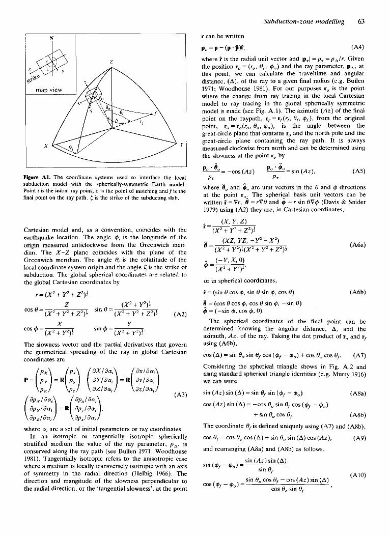
Subduction-zone modelling 63

N I T

Figure Al. The coordinate systems used to interface the local subduction model with the spherically-symmetric Earth model. Point i is the initial ray point, o is the point of matching andfis the final point on the ray path. 5 is the strike of the subducting slab.

Cartesian model and, as a convention, coincides with the earthquake location. The angle Cpj is the longitude of the origin measured anticlockwise from the Greenwich meri- dian. The X - Z plane coincides with the plane of the Greenwich meridian. The angle Oj is the colatitude of the local coordinate system origin and the angle [ is the strike of subduction. The global spherical coordinates are related to the global Cartesian coordinates by

r = (x’ + Y’ + z’)t (X’ + Y2)t

sin 8 = Z

(X’ + Y2 + Z”)t cos 8 = (x‘ + Y2 + z2)i (A2)

X Y sin Cp = (X’ + Y’)i (X’ + Y2)+’

cos Cp =

The slowness vector and the partial derivatives that govern the geometrical spreading of the ray in global Cartesian coordinates are

where ai are a set of initial parameters or ray coordinates. In an isotropic or tangentially isotropic spherically

stratified medium the value of the ray parameter, p a , is conserved along the ray path (see Bullen 1971; Woodhouse 1981). Tangentially isotropic refers to the anisotropic case where a medium is locally transversely isotropic with an axis of symmetry in the radial direction (Helbig 1966). The direction and mangitude of the slowness perpendicular to the radial direction, or the ‘tangential slowness’, at the point

r can be written

where i is the radial unit vector and /ptI = p z = p a / ‘ . Given the position ro = (To, O,, Cpo) and the ray parameter, pA, at this point, we can calculate the traveltime and angular distance, (A), of the ray to a given final radius (e.g. Bullen 1971; Woodhouse 1981). For our purposes ro is the point where the change from ray tracing in the local Cartesian model to ray tracing in the global spherically symmetric model is made (see Fig. A.l). The azimuth (Az) of the final point on the raypath, r, = r f (r f , Of, Cp,), from the original point, ro =ro(r,, 8,, Go), IS the angle between the great-circle plane that contains ro and the north pole and the great-circle plane containing the ray path. It is always measured clockwise from north and can be determined using the slowness at the point ro by ..

where 6, and 3, are unit vectors in the 8 and Cp directions at the point r, The spherical basis unit vectors can be written i = Vr, 8 = r V 8 and 3 = r sin OVCp (Davis & Snider 1979) using (A2) they are, in Cartesian coordinates,

i = ( X , y, Z ) (X’ + Y2 + Z2)i

8 = .. ( X Z , Y Z , - Y‘ - X’) (X’ + Y’)t(X’ + Y’ + Z’)i

or in spherical coordinates,

i = (sin 8 cos 9, sin 8 sin @, cos 8)

3 = (cos 8 cos ~ p , cos 8 sin 4, -sin 8) 3 = (-sin 4, cos c ~ , o ) .

The spherical coordinates of the final point can be determined knowing the angular distance, A, and the azimuth, Az, of the ray. Taking the dot product of ro and r, using (A6b),

cos (A) = sin 8, sin 8, cos (4, - C p o ) + cos 8, cos 8,. (A7)

Considering the spherical triangle shown in Fig. A.2 and using standard spherical triangle identities (e.g. Murry 1916) we can write

(A6b)

sin (Az) sin (A) = sin 8, sin (Cp, - Cp,) (A8a)

+ sin 8, cos (A8b)

(A9)

cos (Az) sin (A) = -cos 8, sin 0, cos (Cp, - 4,)

The coordinate 8, is defined uniquely using (A7) and (A8b),

cos 8, = cos 8, cos (A) + sin 8, sin (A) cos (Az),

and rearranging (A8a) and (A8b) as follows,

sin (Az) sin (A)

sin 8, cos 8, - cos (Az) sin (A) cos 8, sin Of

sin (Cp, - $0) =

COS (4, - 4,) =

sin (A10)

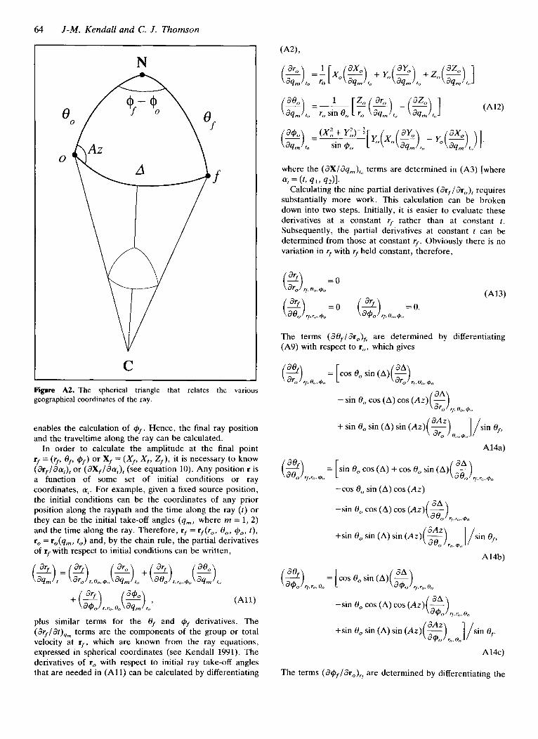
64 J-M. Kendall and C. J . Thomson

N

v

C Figure A2. The spherical triangle that relates the various geographical coordinates of the ray.

enables the calculation of 4,. Hence, the final ray position and the traveltime along the ray can be calculated.

In order to calculate the amplitude at the final point r, = (9, 0,, @) or Xf = (X,, X,, Z,) , it is necessary to know (&,/daJ, or (dX,/da;), (see equation 10). Any position r is a function of some set of initial conditions or ray coordinates, cu,. For example, given a fixed source position, the initial conditions can be the coordinates of any prior position along the raypath and the time along the ray (t) or they can be the initial take-off angles (qm, where rn = 1, 2) and the time along the ray. Therefore, rf = rf(ro, O,, Go, f), r, = ro(qm, to) and, by the chain rule, the partial derivatives of r, with respect to initial conditions can be written,

plus similar terms for the Of and @, derivatives. The (dr,/dt),, terms are the components of the group or total velocity at r f , which are known from the ray equations, expressed in spherical coordinates (see Kendall 1991). The derivatives of t, with respect to initial ray take-off angles that are needed in ( A l l ) can be calculated by differentiating

where the (dX /dqm)r , terms are determined in (A3) [where

Calculating the nine partial derivatives ( dr,/drc,)r requires substantially more work. This calculation can be broken down into two steps. Initially, it is easier to evaluate these derivatives at a constant rf rather than at constant t. Subsequently, the partial derivatives at constant t can be determined from those at constant r f . Obviously there is no variation in r, with rf held constant, therefore,

a; = ( 4 41, qJ1.

The terms (d6,/dr,),, are determined by differentiating (A9) with respect to r,, which gives

A14a)

-cos 8, sin (A) cos (Az)

-sin 8, cos (A) cos (Az)

dAz +sin e, sin (A) sin (A.)(-) ]/sin of,

300 T".+<,

A14b)

A14c)

The terms (d@,/dr,), are determined by differentiating the

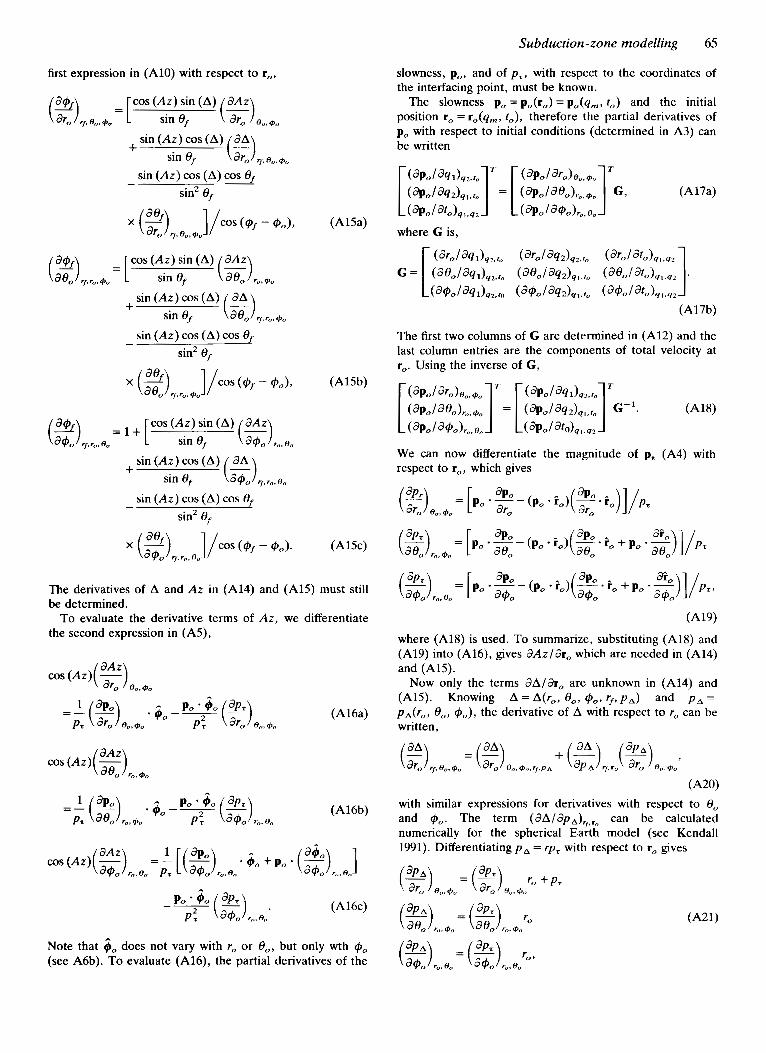
Subduction-zone modelling 65

first expression in (A10) with respect to ro,

+ sin ef

sin (Az) cos (A) cos 8, sin2 ef

-

+ sin (Az) cos (A) cos Or

sin2 ef

+ sin (Az) cos (A) cos 8,

sin2 ef

slowness, p,, and of pr, with respect to the coordinates of the interfacing point, must be known.

The slowness p, = po(ro) = p,(q,, to ) and the initial position ro = r,(q,, to ) , therefore the partial derivatives of po with respect to initial conditions (determined in A3) can be written [ ( *o/ aq 1 L. r ,, ] (dpo/ % J q l , r o = [ ;Z;;~,Z;~] z- G , (apo / ato),, . q 2

where G is,

(A17a)

(*,/a@ )

1 (are/ d q l ) q 2 , r o (are/ %2)q2,r0 (3ro/ ato)ql . q 2

( a e o / % l ) q 2 , r o (aeo/%z)q, ,r , , ('eo"'o)ql,w . (a@,/ % J q z . r o ( d @ o / d q z ) q l , r o ( d@o 1 1.42

(A17b)

The first two columns of G are determined in (A12) and the last column entries are the components of total velocity at r,. Using the inverse of G, [ ~ ~ o ~ ~ ~ O ~ e O , ~ O ] r = [ ( a ~ o ( d P / b O l ) q 2 , r ] T / 3 q J y I,r,, G - '.

We can now differentiate the magnitude of pt (A4) with respect to r,, which gives

('418) (*,I a%),, $.

(apo/~@o),,80 ( apO/ w, 1.42

The derivatives of A and Az in (A14) and (A15) must still be determined.

To evaluate the derivative terms of Az, we differentiate the second expression in (A5),

(A16b)

Note that 6, does not vary with ro or Oo, but only wth Go (see A6b). To evaluate (A16), the partial derivatives of the

(A19)

where (AM) is used. To summarize, substituting (A18) and (A19) into (A16), gives dAz /dro which are needed in (A14) and (A15).

Now only the terms dA/dro are unknown in (A14) and (A15). Knowing A = A(r,, Oo, Go, rf, p A ) and pa = pa(',, O,, @,), the derivative of A with respect to r, can be written,

( E ) r r , 0,. +" = ( E ) e o . + c , . r f , p , + (3 r,, re) 8,. rp<:

(A201 with similar expressions for derivatives with respect to 0, and Go. The term ( d A / d ~ ~ ) , ~ , . , , can be calculated numerically for the spherical Earth model (see Kendall 1991). Differentiating pa = rp, with respect to r, gives

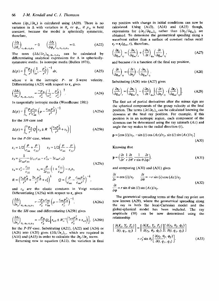
66 J-M. Kendall and C. J . Thomson

where (dp,/dr,) is calculated using (A19). There is no variation in A with variation in 0, or Cp,, if pa is held constant, because the model is spherically symmetric, therefore,

The term ( ~ A / ~ r o ) e o , c p o ~ r f , p A can be calculated by differentiating analytical expressions for A in spherically- symmetric media. In isotropic media (Bullen 1971),

where v is the isotropic P- or S-wave velocity. Differentiating (A23) with respect to ro gives

In tangentially isotropic media (Woodhouse 1981)

A(p) = rp# ( p - 7) % P i -1 rc, r C44

for the SH-case and

for the P-SV-case, where

s1=1 /2 -+- s 2 = 1 / 2 (p, C:l (CY4 c 9

(A25a)

(A25 b)

and cij are the elastic constants in Voigt notation. Differentiating (A25a) with respect to r, gives

(A26a)

for the SH-case and differentiating (A25b) gives

for the P-SV-case. Substituting (A21), (A22) and (A24) or (A26) into (A20) gives (6'A/&o)rf, which are required in (A14) and (A15) in order to calculate the 3rf/3r, terms.

Returning now to equation (Al l ) , the variation in final

ray position with change in initial conditions can now be calculated. Using (A13), (A14) and (A15) though, expressions for ( 3rf/dq,)rf rather than ( 3rf/3qm), are obtained. To determine the geometrical speading along a wavefront rather than a surface of constant radius recall rf = rf(qm, t ) , therefore,

(21rf = (Zit + (2IqjEIr; and because t is a function of the final ray position,

Substituting (A28) into (A27) gives

The first set of partial derivatives after the minus sign are the spherical components of the group velocity at the final position. The terms (3t/3rf) ,f can be calculated knowing the slowness at the final ray position. For example, if this position is in an isotropic region, each component of the slowness can be determined using the ray azimuth (Az) and angle the ray makes to the radial direction ( i) ,

p = [cos (i)/vf, -sin ( i ) cos (Az ) / v f , sin (i) sin ( A z ) / v f ]

(A30)

Knowing that

at 1 at 1

and comparing (A30) and (A31) gives

at at - = cos (i) /vf dr a0

at _- - r sin 0 sin (i) sin ( A z ) / v f . a@

- = -r sin ( i ) cos (Az) /v f

( A 3 4

The geometrical spreading terms at the final ray point are now known (A29), where the geometrical spreading along the ray in both the local-Cartesian model and the global-spherical model has been included. The ray amplitude (10) can be now determined using the relationship