87
The Predictability of GARCH-Type Models on the Returns
Volatility of Primary Indonesian Exported Agricultural
Commodities
Saarce Elsye Hatane
Accounting Department, Petra Christian University
Email: [email protected]
ABSTRACT
Agricultural sector plays an important role in Indonesia‟s economy; especially for the
plantation sub-sector contributing high revenues to Indonesia‟s exporting sectors. The
primary agricultural commodities in Indonesian export discussed in this study would be
Crude Palm Oil (CPO), Natural Rubber TSR20, Arabica Coffee, Robusta Coffee, Cocoa, White
Pepper and Black Pepper. Meanwhile, the returns volatility nature of agricultural commodity
is famous. The volatility refers to heteroscedasticity nature of the returns which can be
modeled by GARCH-type models. The returns volatility can be describe by the residual of the
mean equation and volatility of error variances in the previous periods. The aims of this study
are to examine the predictability of GARCH-type models on the returns volatility of those
seven agricultural commodities and to determine the best GARCH-type models for each
commodity based on the traditional symmetric evaluation statistics. The results find that the
predictability of ARCH, GARCH, GARCH-M, EGACRH and TGARCH, as type of GARCH
models used in this study, are different for each commodity.
Keywords: ARCH, GARCH, GARCH-M, EGACRH, TGARCH, returns volatility, residuals,
agricultural commodity.
INTRODUCTION
Low returns and high risks are two issues
faced by agricultural commodity producers as
mentioned by UK‟s Department for International
Development (DFID) on its 2004 report. According
to the DFID, those two problems occur due to the
less rapid growth of agricultural commodities‟
prices compared to those of manufactured pro-
ducts, and the price volatility in agricultural
commodities. Generally, commodities, especially
agricultural commodities, are well known for their
prices volatility patterns (Newbery, 1989). The
DFID argues that developing countries which are
highly dependable on agricultural commodities
should try to decrease their dependency on those
commodeties. One such developing country, which
will be the focus of this article, is Indonesia.
Agriculture is traditionally the main sector of
Indonesia‟s economic activity. Until 1960, it
represented 50% of Indonesian‟s Gross Domestic
Product (GDP), as shown in Figure 1. The decline
of the percentage inthe GDP since 1966 was due to
the effort to reduce Indonesian overdependence on
farmers. In the period of OrdeBaru, which was
headed by Soeharto (Indonesian second president),
the economy development were not just focused on
agriculture, but also on other sectors such as
manufacturing, electricity, construction, services
and finance sectors (Djamin, 1989). Figure 1 shows
that in the percentage of agriculture roles on GDP
decreased from about 50% in 1960 to about 16% in
1996. The percentage increased to be 18% in 1998
and 19% in 1999.
Three decades of stable progress in Indone-
sian agricultural development were suddenly dis-
turbed by financial and environmental shocks in
1997 (Daryanto, 1999). Daryanto also mentioned
that those conditions caused food insecurity, but in
opposite to food crops, the Asian crisis gave positive
impacts on farm non-food crops (plantations) and
forestry. As high export-oriented and low import-
oriented subsectors, they enjoyed the prizes from
the Asian crisis due to the Indonesian Rupiah
(IDR) depreciation. After the Asian financial crisis
in 1998, the good performance of agricultural
exports was one factor, from agricultural sector,
that saved Indonesia from the crisis (Basri, 2002).
Discussion on the degree of commodity price
volatility has become one remarkable topic, and

JURNAL AKUNTANSI DAN KEUANGAN, VOL. 13, NO. 2, NOVEMBER 2011: 87-97
88
attracted attention of researchers in economic and
financial fields. For instance, Kroner et al. (1993);
Sekhar (2003, 2004); O‟Connor et al. (2009); and
Alom et al. (2010), they reported that international
prices of agricultural commodities are one of the
most volatile prices in international market.
Deaton (1999) argued that having a better under-
standing about commodity prices characteristics is
extremely important for developing countries that
depend on commodity exports or that import huge
amounts of food. Many researchers have employed
and extended the ARCH/GARCH methodology to
examine various commodities price volatility
issues. For example, Alom et al. (2010); Sumar-
yanto (2009); O‟Connor et al. (2009); Zheng et al.
(2008); Apergis and Rezitis (2003, 2011); Yang et
al. (2001); and Beck (2001), theyapplied GARCH-
type models to analyze the price volatility of
agricultural products. Some empirical studies
reported the existence of price volatility in futures
prices and spot prices of some commodities.
Mahesha (2011) reported that international spot
prices of cardamom, ginger and pepper from India
indicated long persistence and volatility clustering.
Yang et al. (2001) also reported that some US
commodities, i.e. corn, oat, soybeans, wheat and
cotton, had price volatility feature, both for futures
prices and spot prices.
Measuring and Forcasting Volatility
Volatility comes from the term of „volatile‟. This
term refers to conditions that unstable prices tend
to vary and are difficult to forecast. The key words
in volatility are variability and uncertainty (Engle,
2003). Volatility is an important variable for port-
folio management, option pricing and market regu-
lations (Poon and Granger, 2003). The relationship
between volatility and option price is positive.
When volatility increases, then the option price will
also increase. Thereby, information about price
volatility is useful in estimating more precise and
reasonable option price. Some empirical studies
reveal that price volatility can be measured by
standard deviation and coefficient of variation of
asset price concerned.
According to Engle (1982), Bollerslev (1986)
and Taylor (1986), the particular non-linear models
that have been proven very useful in finance are
the autoregressive conditional heteroscedasticity
(ARCH) and generalized autoregressive conditional
heteroscedasticity (GARCH) models.
Thus far, the forecasting methods of time
series data are autoregressive (AR), moving ave-
rage (MA), or a combination of both (either ARMA
or ARIMA). Results obtained from those forecast-
ing methods will have high accuracy if the assump-
tion of homoscedasticity in the error variances
fulfilled. However, some problems arise when those
forecasting methods are applied to commodity
market which its price fluctuations tend to be
bunches, like happened in stock exchange market
or futures exchange market. The bunched features
characterized the existence of large changes (e.g.
large returns) are expected to follow large changes,
and conversely, small changes to follow small
changes (Diebold, 2004). These characteristics are
known as heteroscedasticity. In time series data
which have heteroscedasticity variances, the
variances of error do not depend on their inde-
pendent variable. Those variances are changing
along with the time change. Those time series data
Source: Indicators Data of the World Bank. Data was modified by the author.
Figure 1. Indonesian Agriculture, Value Added - % of GDP

Saarce: The Predictability of GARCH-Type Models
89
have volatility character which is heteroscedasti-
city, because their error variances depend on the
volatility of past errors. Data that have heteros-
cedasticity nature can be modeled by ARCH and
GARCH models. ARCH/GARCH models utilize
heteroscedasticity in the error variance appropria-
tely in order to get the more efficient estimators.
Good AR and MA models can be suitable for ARCH
models, particularly in modeling the means‟ changes
(Shephard, 1996).
Previous Study
In 2001, Beck analyzed the ARCH process for
twenty commodities, storable and non-storable commodities, by using annual spot market data..
The results showed that prices volatility of each commodity was modeled by different type of
ARCH/GARCH models. In summary, price vola-tility which was examined by ARCH/GARCH models mostly found in storable commodities. Sumaryanto (2009) analyzed retail price volatility
of some Indonesian food commodities using ARCH/ GARCH models. From the overall estimateon results, it appeared that the most appropriate model for rice, red chili and shallot was ARCH (1);
while for sugar and wheat flour was GARCH (1,1). However, ARIMA was the fitted model for cooking oil and egg. Yang et al. (2001) examined the effect of agricultural liberalization policy, the Federal
Agricultural Improvement and Reform (FAIR) Act of 1996, towards US agricultural commodity prices volatility using GARCH models. The commodities
were corn, oat, soybeans, wheat and cotton. Total
observations were 1695 active traded cash and futures prices from 1 January 1992 to 30 June 1998. Finally, the paper concluded that GARCH (1,1) model had done adequate job in describing the
data-generating process of cash and futures prices of each commodity. Mahesha (2011) investigated international price volatility of Indian of spices
exports. This study applied GARCH (1,1) model to estimate the time varying conditional variances. The result showed that there was a high volatility clustering in cardamom, ginger and pepper.
Pinisakikool (2009) applied ARIMA-GARCH and ARIMA-TARCH with dummy variable to inves-tigate whether futures traded in The Agricultural Futures Exchange of Thailand (AFET) could sta-
bilize the spot price volatility or not. The results showed that spot price volatility model of the commodities studied were compatible with GARCH (1,1) and TARCH (2, 2).
RESEARCH METHODS
The independent variables in this study are
errors (residuals) from the mean equations (ARMA
model) and volatility in the previous periods (t-1);
while the dependent variable is the price returns
volatility in current period (t). The objects used in
this study are CPO, Natural Rubber TSR20,
Arabica Coffee, Robusta Coffee, Cocoa, White
Pepper and Black Pepper. The specific purpose in
this study is the predictability on GARCH-type
models in describing the causal relationship bet-
ween those variables. Since there are five type
models of GARCH-type models used, which are
ARCH; GARCH; GARCH-M; EGARCH; and
TGARCH, and seven objects, this study does
exploratory study to test whether those GARCH-
type models can be used to predict the volatility of
return prices of each commodity. All of the data
used are weekly spot price series of those seven
commodities from January 1, 2005 to June 30,
2011. The weekly spot price in this study is the
closing price of immediate cash price on the last
trading day of each week. Thus, total observations
of each commodity are 338 weekly spot prices or
equal to 337 observations of weekly spot price
returns.
Constructing ARMA Model
Constructing ARMA model can be done only if
the time series data is stationary. ARMA model is
critical in generating a good GARCH forecasting
model. There are four steps from Brooks (2008)
used in this study to build the ARMA model. The
identification process uses graphical procedures to
determine the most appropriate specification. The
graphics are plotting the data overtime and also
the correlogram of autocorrelation function (ACF)
and partial correlation function (PACF). ACF is
used to the moving average (MA) model, while the
PACF is used to predict the AR model. The
estimation of ARMA models from the combination
of AR and MA. The diagnostic process that testing
the serial correlation problem and heteroscedasti-
city problem. The serial correlation problem should
be solved first before testing the heteroscedasticity
problem. From all of significant ARMA models, the
best ARMA model was selected using Bayes
Information Criterion (BIC) or known as Schwarz
Information Criterion (SIC). The model with the
lowest value of SIC should be chosen.
The GARCH Building Process
After determining the mean equation from
ARMA model, the building of volatility equations
in GARCH forms begins. The GARCH-type models
employed in this study are:
ARCH (q) Model. It was proposed by Engle in
1982 to capture volatility persistence in inflation.
JURNAL AKUNTANSI DAN KEUANGAN, VOL. 13, NO. 2, NOVEMBER 2011: 87-97
90
The ARCH model does not utilize past standard
deviations, but formulate conditional variance (2
tσ )
of asset returns by maximum likelihood proce-
dures. The conditional variance equation is:
quα...2uα1uαασ 2
tq
2
t2
2
t10
2
t (1)
GARCH (p,q) Model.According to Bollerslev
(1986) and Taylor (1986), the high-order ARCH(q)
process is more proximate to model GARCH (p,q).
The additional dependencies on the residual
variance are permitted on p lags of past 2
tσ as
shown below: 2
p-tp
2
1-t1
2
q-tq
2
1-t10
2
t σβ...σβuα...uαασ (2)
GARCH-M (p, q) Model. It was introduced by
Engle, Lilien and Robin in 1987, includes the
conditional variance or standard deviation into the
mean equation. The conditional variance equation
is: 2
p-tp
2
1-t1
2
q-tq
2
1-t10
2
t σβ...σβuα...uαασ (3)
EGARCH (p, q) Model. It was introduced by
Nelson in 1991. The EGARCH (p,q) denotes condi-
tional variance in logarithmic form. The equation
is:
p
1j
p
1i2
j-t
jt
j2
1-t
1t2
i-ti
2
t
σ
u
σ
u)σ(βω)(σ lnln
(4)
TGARCH (p, q) Model.This model was
introduced by Zakoïan in 1994. It was developed
from Threshold Arch (TARCH or GJR) model by
Glosten, Jaganathan and Runkle in 1993. The
equation for conditional variance is:
q
1j
p
1i
ul 2
j-tj1t1t
2
i-ti0
2
t uσβσσ (5)
lt-k = 1 if ut-k < 0; lt-k = 0 if ut-k > 0
Brooks (2008) explained three steps involved
in estimating GARCH-type models. Determine the
appropriate equations for the mean and the
variance; determine the log-likelihood function
(LLF) to maximize under a normality assumption
for the disturbances; and computer program will
maximize the function and generate parameter
values that maximize the LLF and also will
construct their standard errors.In order to have
significant GARCH-type models, the probability
value of each coefficient in those models has to be
compared with critical values (1%, 5% and 10%). If
there is one insignificant coefficient in the esti-
mated model, except the constant term, the null
hypothesis will be failed to be rejected. It means
that the model cannot be used to predict the
volatility. In vice versa, if all of the coefficients in
the model are significant, the null hypothesis will
be rejected. It means that the model can be used to
predict the volatility. However, this condition does
not work in the constant term.
The Evaluation Process
The first step in evaluating the prediction
power among GARCH-type models is measuring
the “true or realized volatility.” Brooks (2008)
explained that true or ex post volatility is the actual
historical volatility of a security‟s price. Ex post
volatility measurement used in this study based on
formula proposed by Day and Lewis (1992). The
model is expressed as follow: 2
t
2
t γ)(γσ (6)
The best predicting models among the
GARCH-type models are selected by using three
traditional symmetric evaluation statistics. Those
are root mean square error (RMSE), mean absolute
percent error (MAPE) and mean absolute error
(MAE).
RESULTS AND DISCUSSION
The mean values, as shown in Table 1, were
far from one. Those indicate that the data are
stationary around zero. The standard deviation
values, which are far from one, show the diversity
of data which means that each commodity has high
volatility in its price returns. The probability of
Jarque-Bera in all of those commodities shows that
those are not distributed normally. This study used
ADF test statistic to perform the stationary test.
The t-statistic value must be greater than the ADF
test statistic values. Table 2 shows that all of those
seven commodities have t-statistic values greater
than all critical values. It means that the price
return series of those commodities are stationary.
The results of ARMA construction process for each
commodity are shown in Table 3. Although Ara-
bica, Robusta and Black Pepper are shown have no
heteroscedasticity problem, the returns volatility of
those commodities can still be predicted by ARCH
family models (Francq & Zakoian, 2010).
ARCH (q), GARCH (p, q), GARCH-M (p, q),
EGARCH (p, q) and TGARCH (p, q) were analyzed
for each commodity. The q expresses the lag of
error or residual from the mean equation, while the
p expresses the lag of volatility. Each model is
analyzed in four lags of residual and four lags of
volatility. Table 4 to Table 10 shows the results of
the variance equation for each commodity.
Table 4 shows that ARCH model; GARCH
model; GARCH-M model; and TGARCH model can

Saarce: The Predictability of GARCH-Type Models
91
Table 1. Summary of Data Description
Table 2. Summary of Stationary Testing
Table 3. Summary of ARMA Models

JURNAL AKUNTANSI DAN KEUANGAN, VOL. 13, NO. 2, NOVEMBER 2011: 87-97
92
Table 4. The Results of GARCH Construction Process for CPO
Note: * = significant at 1%; ** = significant at 5%; *** = significant at 10%; value in the parenthesis is the p-value
Table 5. The Results of GARCH Construction Process for Natural Rubber TSR20
Note: * = significant at 1%; ** = significant at 5%; *** = significant at 10%; value in the parenthesis is the p-value
Table 6. The Results of GARCH Construction Process for Arabica Coffee
Note: * = significant at 1%; ** = significant at 5%; *** = significant at 10%; value in the parenthesis is the p-value

Saarce: The Predictability of GARCH-Type Models
93
Table 7. The Results of GARCH Construction Process for Robusta Coffee
Note: * = significant at 1%; ** = significant at 5%; *** = significant at 10%; value in the parenthesis is the p-value
Table 8. The Results of GARCH Construction Process for Cocoa
Note: * = significant at 1%; ** = significant at 5%; *** = significant at 10%; value in the parenthesis is the p-value
JURNAL AKUNTANSI DAN KEUANGAN, VOL. 13, NO. 2, NOVEMBER 2011: 87-97
94
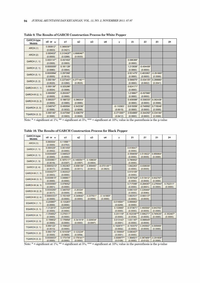
Table 9. The Results of GARCH Construction Process for White Pepper
Note: * = significant at 1%; ** = significant at 5%; *** = significant at 10%; value in the parenthesis is the p-value
Table 10. The Results of GARCH Construction Process for Black Pepper
Note: * = significant at 1%; ** = significant at 5%; *** = significant at 10%; value in the parenthesis is the p-value

Saarce: The Predictability of GARCH-Type Models
95
be used to predict the volatility of spot price returns
of CPO. Table 5 shows that ARCH model; GARCH
model; GARCH-M model; and EGARCH model can
be used to predict the volatility of spot price returns
of TSR20. Table 6 shows that GARCH model;
GARCH-M model; EGARCH model; and TGARCH
model can be used to predict the volatility of spot
price returns of Arabica Coffee. Table 7 shows that
GARCH model; GARCH-M model; EGARCH
model; and TGARCH model can be used to predict
the volatility of spot price returns of Robusta
Coffee. Similar to Arabica Coffee and Robusta
Coffee, ARCH model also cannot be used to predict
the volatility of Cocoa spot price returns. Table 8
shows that GARCH model; GARCH-M model;
EGARCH model; and TGARCH model can be used
to predict the volatility of spot price returns of
Cocoa. Table 9 shows that ARCH model; GARCH
model; GARCH-M model; EGARCH model; and
TGARCH model, can be used to predict the
volatility of spot price returns of White Pepper.
Similar to White Pepper, all of the GARCH-type
models in this study were fit as volatility prediction
models for Black Pepper‟s spot price returns
volatility.
This study has chosen the most recent 67
weeks, which are about 20% of total observations of
each commodity, as the periods to evaluate the
predictability of the significant GARCH-type
models (Brook, 2008). The evaluation process
results are shown in Table 11.
With respect to RMSE criterion, ARCH is the
best prediction model for returns volatility of White
Pepper; GARCH-M is the best prediction model for
returns volatility of CPO; and EGARCH is the best
prediction model for returns volatility of Natural
Rubber TSR20, Arabica Coffee, Robusta Coffee,
Cocoa and Black Pepper. In this criterion, GARCH
model and TGARCH model are not selected as the
best prediction model of any commodities.
With respect to MAPE criterion, GARCH is
the best prediction model for returns volatility of
Robusta Coffee; GARCH-M is the best prediction
model for returns volatility of Arabica Coffee and
Cocoa; EGARCH is the best prediction model for
returns volatility of TSR20, White Pepper and
Black Pepper; TGARCH was the best prediction
model for returns volatility of CPO. In this
criterion, ARCH is not selected as the best
prediction model of the returns volatility of any
commodities.
With respect to MAE criterion, GARCH-M is
the best prediction model for returns volatility of
CPO and White Pepper; and EGARCH is the best
prediction model for returns volatility of TSR20,
Arabica Coffee, Robusta Coffee, Cocoa and Black
Pepper. In this criterion, ARCH model, GARCH
model and TGARCH model are not selected as the
best prediction models of the returns volatility of
any commodities.
The predictability of ARCH model in Indone-
sian exported agricultural commodities, as had
been discussed in this study, is supported by the
studies of Beck (2001) and Sumaryanto (2009).
Their studies found that ARCH model was fit to
predict the volatility of commodity price returns.
Table 11. The Summary of Best GARCH-Type Models
JURNAL AKUNTANSI DAN KEUANGAN, VOL. 13, NO. 2, NOVEMBER 2011: 87-97
96
Furthermore, the predictability of GARCH model
in Indonesian exported agricultural commodities is
supported by Beck (2001), Yang et al. (2001),
Swaray (2002), Zheng et al. (2008), Sumaryanto
(2009), Pinisakikool (2009), O‟Connor et al. (2009)
and Mahesha (2011). EGARCH model is found as
the best model in predicting the spot price returns
volatility of Natural Rubber TSR20, Arabica
Coffee, Robusta Coffee, Cocoa, White Pepper and
Black Pepper. It seemed that EGARCH model is
the best prediction model for all commodities,
except CPO. The predictability of EGARCH Model
in predicting the returns volatility of Indonesia
exported agricultural commodities is supported by
the studies of Swaray (2002) and Zheng et al.
(2008). TGARCH model is found as the best model
in predicting the returns volatility of CPO. The
result is supported by studies of Huang et al.
(2008) and Pinisakikool (2009).
CONCLUSIONS
High level of volatility can indicate that a
commodity has a high risk. The results of this
study can give benefit to investor and prospective
investors to manage their portfolios and asses their
investment risks related to those seven commo-
dities. In order to deal with the relatively high
volatility level of Indonesia commodities spot price
returns, financial instruments such as forwards
and futures markets may be desirable. The results
in this study give insight to the market players
about timing of hedging.
The information in this study also can give
additional information to Indonesian government
in increasing cash inflow to the country, since
Indonesia is an international major player in those
seven commodities markets (Agriculture Data
Center, 2011). The increase of cash inflow can be
realized by maintaining the existence of the
commodities, quantities and quality, in fulfill the
market demand. The welfare of farmers and small
private sectors of those seven commodities should
be put into account. Government can give them
insight and encouragement to add values of those
commodities through manufacturing sector. They
can manufacture those commodities further to be
another half or full finished goods forms. Therefore,
when the market prices become too high which
lead to the decrease of demand, they will survive
from the manufactured products of those commo-
dities.
The information from this study can also be a
useful reference for economist, financial analysts
and researchers, who are interested in Indonesian
agricultural export commodities and also inte-
rested in the application of GARCH-type models.
The application of GARCH-type models in agricul-
tural fields could be a significant contribution to
quantitative analysis of financial fields.
For the future researches, the prediction of
risk by GARCH-type models used in this study
could also be applied in other research objects, such
as fixed income financial asset markets, currency
markets, stock markets, other commodities mar-
kets, tourism, etc. The future researches also can
use advanced type of GARCH models in order to
get more specific results.
REFERENCES
Agriculture Data Center (2011), Monthly Bulletin:
Indikator Makro Sektor Pertanian, (Macro
Indicators of Agricultural Sector), Jakarta:
Data Center and Information System of Indo-
nesian Agriculture Ministry, August Edition.
Alom, M.D.F., Ward, B.D. & Hu, Baiding (2010),
“Cross Country Mean and Volatility Spillover
Effects of Food Prices: Evidence for Asia and
Pacific”, International Review of Business
Research Papers, 6 (2), 334-355.
Apergis, N., &Rezitis, A. (2003), “Agricultural Price
Volatility Spillover Effects: The Case of
Greece”. Journal of Agricultural and Applied
Economics, 43, 95-110.
Apergis, N., &Rezitis, A. (2011), “Food Price Volati-
lity and Macroeconomic Factors: Evidence
from GARCH and GARCH-X Estimates”,
European Review of Agricultural Economics,
30, 389-406.
Basri, F. (2002), Perekonomian Indonesia (Indonesian
Economy), Jakarta: Erlangga.
Beck, Stacie (2001), “Autoregressive Conditional
Heterocedasticity in Commodity Spot Prices”,
Journal of Applied Econometrics, 16, 115-132.
Bollerslev, T. (1986), “Generalized Autoregressive
Conditional Heteroscedasticity”, Journal of
Econometrics, 31, 307-327.
Brooks, Chris. (2008), Introductory Econometrics
for Finance, New York: Cambridge University
Press, 2nd edition.
Commodity Futures Trading Regulatory Agency
(CoFTRA) (2011), Forward-Futures-Spot Com-
modities Values Data, Retrieved July 04, 2011 from http://www.bappebti.go.id/?pg=harga_bursa.
Daryanto, Arief (1999), Indonesia’s Crisis and the
Agricultural Sector: the Relevance of Agri-
cultural Demand-Led Industrialization,
UNEAC Asia Paper, 2. Australia.
Deaton, Angus (1999), “Commodity Prices and
Growth in Africa”, Journal of Economic
Perspectives, 13, 23-40.
Diebold, F.X. (2004), “The Nobel Prize for Robert F.
Engle”, Scandinavian Journal of Economics,
106, 165-185.
Saarce: The Predictability of GARCH-Type Models
97
Djamin, Zulkarnain (1989), Perekonomian Indone-
sia (Indonesian Economy), Jakarta: Published
Center of Economics Faculty, University of
Indonesia.
Engle, R.F. (1982), “Autoregressive Conditional
Heteroscedasticity with Estimates of the
Variance of United Kingdom Inflation”,
Econometrica, 50, 987-1007.
Engle, R.F. (2003), Risk and Volatility: Econometric
Models and Financial Practice, Nobel Prize in
Economics Documents 2003-4, Nobel Prize
Committee.
Engle, R.F., Lilien, L.D., & Robins, R. (1987), “Esti-
mation of Time Variying Risk Premiums in
the Term Structure”, Econometrica, 55, 391-408.
Francq, C., Zakoian, J.M. (2010), Garch Models:
Structure, Statistical Inference and Financial
Applications, Wiley.
Huang, B.W., Yeh, C.Y., Chen, M.G., Lin, Y.Y. &
Shih, M.L. (2008), Threshold and Asymmetric
Volatility in Taiwan Broiler Farm Price
Change, In Proceedings of the Third Inter-
national Conference on Convergence and
Hybrid Information Technology (pp. 1037-
1042), Retrieved from IEEE Computer Society
(DOI 10.1109/ICCIT.2008.71).
Kroner, Kenneth F., Kneafsey, Kevin P. & Claes-
sens, S. (1995), “Forecasting Volatility in
Commodity Markets”, Journal of Forecasting,
14, 77-95.
Mahesha, M. (2011), “International Price Volatility
of Indian Spices Exports–An Empirical
Analysis Asia and Pacific”, Journal of Research
in Business Management, 2, 110-116.
Nelson, D.B. (1991), “Conditional Heteroskedas-
ticity in Asset Returns: A New Approach”,
Econometrica, 59(2), 347-370.
Newbery, D.M. (1989), “The Theory of Food Price
Stabilization”, The Economic Journal, 9,
1065-1082.
O‟Connor, D., Keane, M. & Barner, E. (2009), Mea-
suring Volatility in Dairy Commodity Prices.
The 113th European Association of Agri-
cultural Economist Seminar, Greece, 1-16.
Pinisakikool, Teerapong (2009), “Do Futures Sta-
bilize the Volatility of the Agricultural Spot
Prices? Evidence from Thailand”, Euro Econo-
mica, 22 (1), 47-56.
Poon, S.H., and Granger, J. (2003), “Forecasting
Volatility in Financial Markets: A Review”,
Journal of Economic Literature, XIL, 478-539.
Sekhar, C.S.C. (2003), Volatility of Agricultural
Prices–An Analysis of Major International
and Domestic Markets, Indian Council for
Research on International Economic Rela-
tions, Working Paper No. 103.
Sekhar, C.S.C. (2004), “Agricultural Price Volatility
in International and Indian Markets”, Eco-
nomic and Political Weekly, 39, 4729-4736.
Shephard, N. (1996), Statistical Aspect of ARCH
and Stochastic Volatility, In Cox, D.R.,
Hinkley, E.V., and Barndoff-Nielson, O.E. (Eds),
Time Series Models in Econometrics, Finance
and Other Fields, New York: Chapman and
Hall.
Sumaryanto (2009), “Retail Price Volatility Analysis
of Some Food Commodities Using ARCH/
GARCH Model”, Journal of Agro Economic
Indonesia, 27, 125-163.
Swaray, R.B. (2002), Volatility of Primary Commodity
Prices: Some Evidence from Agricultural
Exports in Sub-Saharan Africa, The Univer-
sity of York, Discussion Papers in Economics,
06.
Taylor, S.J. (1986), Modelling Financial Rime Series.
Chichester: John Wiley.
The Agriculture and Natural Resources Team of
the UK Department for International Deve-
lopment (DFID) (2004), Rethinking Tropical
Agricultural Commodities, The United King-
dom: The Report of DFID.
The World Bank (2011), Agriculture, value added
(% of GDP), World Bank national accounts
data, and OECD National Accounts data files,
Retrieved November, 02, 2011 from http://
data.worldbank.org/indicator/NV.AGR.TOTL.
ZS/countries/ID?display=graph.
Yang, J., Haigh, Michael S. & Leatham, David J.
(2001), “Agricultural Liberalization Policy and
Commodity Price Volatility”, Applied Economic
Letters, 8, 593-598.
Zakoian, J.M. (1994), “Threshold Heteroscedastic
Models”, Journal of Economic Dynamic and
Control, 12, 193-202.
Zheng, Y., Kinnucan, H.W. & Thompson, H. (2008),
“News and Volatility of Food Prices”, Applied
Economics, 40, 1629-1635.
Recommended