The Impact of Light Rail Transit-Oriented Development
on Residential Property Value in Seattle, WA
Ze Wang
A thesis
submitted in partial fulfillment of the
requirements for the degree of
Master of Urban Planning
University of Washington
2016
Committee:
Qing Shen
Christopher Bitter
Program Authorized to Offer Degree:
Urban Design and Planning

©Copyright 2016
Ze Wang
University of Washington
Abstract
The Impact of Light Rail Transit-Oriented Development on Residential Property Value in
Seattle, WA
Ze Wang
Chair of the Supervisory Committee:
Professor Qing Shen
Urban Design and Planning
The study seeks to investigate the impact of transit-oriented development (TOD) on residential
property values using the case of Link light rail TOD in Seattle. While many previous studies
decompose TOD impact into constituent parts, the study captures the integrated influence of
TOD. Hedonic pricing method is employed and time-series analysis is conducted for three
selected light rail station areas. Dummy variables are designed to reflect TOD proximity and
relevant structural characteristics, locational conditions, as well as social-economic attributes are
identified and controlled in regression models. Results demonstrate that TOD impact is different
across time periods. In pre and during construction periods, TOD does not have statistical
significant influence on the prices of residential properties; in after-construction period, TOD has
significant positive impact on values of residential properties that are located within 0.25-0.50
mile from the light rail station.
Table of Contents
CHAPTER 1 INTRODUCTION .......................................................................................................... 1
CHAPETER 2 LITERATURE REVIEW ............................................................................................. 3
2.1 Price Effects of TOD Characteristics and Other Factors ............................................................... 3
2.1.1 TOD Characteristics ..................................................................................................................... 3
2.1.2 Other Factors ................................................................................................................................ 7
2.2 Analysis Methods .......................................................................................................................... 11
CHAPTER 3 METHODOLOGY ....................................................................................................... 14
3.1 Question and Hypothesis .............................................................................................................. 14
3.2 Conceptual Model ......................................................................................................................... 14
3.3 Statistical Analysis ........................................................................................................................ 16
3.3.1 Hedonic Pricing Analysis ........................................................................................................... 16
3.3.2 Regression Models ..................................................................................................................... 17
Chapter 4 Study Area .......................................................................................................................... 18
4.1 Link Light Rail .............................................................................................................................. 18
4.2 Station Area Overlay District ........................................................................................................ 18
4.3 Study Area Selection and Description .......................................................................................... 20
Chapter 5 Data .................................................................................................................................... 24
5.1 Data Source ................................................................................................................................... 24
5.2 Parcel Extraction ........................................................................................................................... 25
5.3 Variables ....................................................................................................................................... 28
5.3.1 Explanatory TOD Variables ....................................................................................................... 28
5.3.2 Control Variables ....................................................................................................................... 28
5.3.3 Dependent Variable ................................................................................................................... 29
5.3.4 Variable Definitions and Sources .............................................................................................. 30
5.4 Descriptive Statistics ..................................................................................................................... 32
CHAPTER 6 MODEL RESULTS ...................................................................................................... 34

6.1 Pre-Construction Period ................................................................................................................ 34
6.2 During-Construction Period .......................................................................................................... 38
6.3 After-Construction Period ............................................................................................................. 41
CHAPTER 7 CONCLUSION ............................................................................................................. 44
Bibliography ....................................................................................................................................... 46
1
CHAPTER 1 INTRODUCTION
Over the past decades, a growing number of communities have adopted Transit-Oriented
Development (TOD) strategy to help revitalize American cities. TOD is designed typically for
areas centered with a transit station, in order to maximum accessibility and utility of the public
transport services.
Certain design and management principals are employed, giving TOD specific characteristics,
such as high density, high degree of mixed-use, non-motorized friendly networks design, and high
level of transit service (Dittmar and Ohland, 2004). Because of the unique characteristics, TOD
has great influences on its surrounding areas. It is estimated that at an individual station, TOD can
increase ridership by 20% to 40%, and up to 5% overall at the regional level (Arrington, 2005).
Locations next to transit can enjoy increases in land values of over 50% in comparison to locations
away from transit stops (City of Winnipeg, 2011).
Based on the kind of transit service that generates the development, TOD can be classified into
different transit types, including rapid transit TOD, railway TOD, and light rail TOD. In the late
18th century, light rail transit systems were opened in seven U.S. and four Canadian cities. Since
then, light rail transit has been popular being proposed for large and medium-sized metropolitan
areas (Black, 1993). With the increase of light rail construction projects, TOD around light rail
transit is increasingly becoming a standard for the future of TOD in United States. Seattle’s light
rail project, the Link Light Rail was initiated in 1996, two lines of which are operated in 2009
including Tacoma Link, and Central Link. Along with the project, station area plans are conducted
and employed to neighborhoods adjacent to light rail stations. New TOD neighborhoods have
formed gradually around these light rail stations.

2
It is perhaps the right time to investigate the benefits brought by light rail TOD because a lot
of new projects are underway and huge amount of efforts are putting in by local governments and
policy makers. This paper seeks to estimate the capitalization of light rail TOD on residential
properties, which would be beneficial for decision makers from local governments, real estate
companies, and other related agencies to make better financial choices, as well as for the public to
gain a better understanding of what changes TOD can bring to their daily lives.
The study is structured as follows. First, relevant literature is reviewed. Price effects of TOD
related characteristics and other factors affecting property value, as well as previous analysis
methods are compared and summarized. Research question and hypothesis, as well as conceptual
models are then demonstrated in the methodology section. Hedonic pricing method is applied and
time-serious regression models are designed for analysis of pre-during-after construction periods.
The following sections provide the criteria and description of selected study areas, the source and
treatment of data, and the definition and measurement of variables. Finally, model results are
presented and explained, based on which conclusions are drawn and recommendations are
provided in the last chapter.
3
CHAPETER 2 LITERATURE REVIEW
2.1 Price Effects of TOD Characteristics and Other Factors
2.1.1 TOD Characteristics
Economic theory suggests that people are willing to pay a premium for access to
amenities and these amenities are capitalized into property values (Mathur and Ferrell, 2012). A
number of previous literature, studying on the impacts of transit-oriented development (TOD),
decompose TOD impacts into separate components, which are segregated into two categories of
TOD-generated amenities and TOD-generated dis-amenities. Price effects of TOD-generated
amenities contain three major components: transit accessibility effects, pedestrian-friendly
network effects, and mixed-use effects. TOD-generated dis-amenities such as traffic congestion,
noise and air pollution, would likely reduce property values.
Transit accessibility is one major amenity of TOD. An extensive body of literature
explores the price effects of transit proximity.
Economic influence of accessibility starts with the work of Johann von Thunen, who in
1863 theorized about the value of farmland as a function of the land’s relative proximity and,
thus, its accessibility to the market place. Later research translated his work beyond the farmland
context to other types of land use categories, showing similar relationships (Bartholomew and
Ewing, 2011).
Theoretically, as transit service increases land accessibility level, the transportation and
convenience costs of getting to and from the land becomes lower, leading to increased demand
for the land, which raises land values (Landis and Huang, 1995). However, some studies
4
question the applicability of the theory under the consideration that US regions have already
established a well-connected, auto-based transport network accompanied by a spatial dispersion
of both housing and commercial activities, which limits the effectiveness of non-auto modes
(Pucher and Renne, 2003).
Previous research estimating on transit capitalization reveal inconsistent results.
Debrezion, Pels, and Rietveld (2007) conducted a meta-analysis method to generalize conclusion
among 57 studies. They suggested that transit price effects with residential property values
increasing 2.4% for every 250 m closer to a station. While the majority find that transit have a
positive impact on nearby property values, some studies show that the impact is relatively
modest or even negative in some cases. Strand and Vagnes (2001) confirmed a negative
influence of railroad proximity on housing values due to environmental concerns in the case of
Oslo. Hess and Almeida (2006) indicated that transit accessibility does not play a large role in
property values in Buffalo. The existence of light rail influences land values only modestly and
negatively near three stations. Study of Andersson, Shyr, and Fu (2008) shows that high-speed
rail way line has small or negligible effects on residential property prices in Tainan region.
Mathur and Ferrell (2009) examined single-family home prices near four suburban San Francisco
TODs and found no effects from three of them. The negative price effects were explained quite
differently, according to each study’s specific conditions.
Price effects of transit proximity vary with the differences in transit mode, property type,
and measurement methods. According to Hess and Almeida (2006), property near commuter rail
stations has higher premiums than light rail or heavy rail, and property near heavy rail accrues
greater benefits than property near light rail. Effects are greater with proximity measured by
straight line distance, while results are more statistically significant with proximity measured by
5
actual walking distance. Comparison among property types indicates that transit premium for
multifamily housing is much higher than that for single-family housing (Duncan, 2009).
Difference in variable measurements leads to different results as well. Proximity to transport
nodes was associated significantly and positively with single-family values, while proximity to
transport links was negative but not significant (Seo, Golub, and Kuby, 2014).
Mixed-use development provides commercial, institutional, recreational and other
opportunities and services to nearby residents. As an aggregation of mixed-use, TOD promotes
convenience for daily activities and opportunities for employment, which can be capitalized as
housing price premiums.
Price effects of mixed-use depend on a lot of factors, such as property type, land use
scale, mixed-use degree, and proximity to residents. The study of Mathur (2008) indicated that
the accessibility to retail jobs increasing “low quality” housing prices while decreasing “high-
quality” housing prices. Duncan (2009) measured density of population serving employment in
entertainment, food, retail sales and service occupations, representing the amount of non-work
activities within a walkable distance of a parcel. He found that this measure of commercial
activity has a strong and positive impact within 0.1km from transit stations. Lutzenhiser and
Netusil (2001) suggested that housing prices increase with the size of the natural area nearby.
They estimated the optimal size of parks and natural areas to be similar to that of a golf course.
In addition, previous studies demonstrated that the value of all kinds of open space may be
higher in urban areas than in suburban locations. As density increases in urban areas, parks,
green ways, and other natural assets provide increased economic benefits (Acharya and Bennett
2001; Anderson and West 2006).
6
Pedestrian-friendly street design leads to property premiums. It is intuitive that houses
located on quieter-calmer-streets sell at higher prices than those located on busy, noise, high-
trafficked streets (Hughes and Simans, 1992). Study of Song and Knaap (2003) indicated that
people are willing to pay a premium for houses in neighborhood containing interconnected
streets and smaller blocks in Portland, Oregon. One example of Boston’s “Big Dig” project, the
replacement of the elevated Central Artery freeway with an underground facility and the
transformation of the surface to a linear parkway and boulevard, illustrated the premiums based
on economic analysis of Tajima, which suggested that the demolition of the highway should
result in $632 million increase in property values (Bartholomew and Ewing, 2011). Indicators
are developed to estimate the pedestrian-friendly network level, such as density of street
intersections, steepness of terrain, and area dedicated to park and ride lots Duncan (2009).
While many of the previous studies examine price effects of transit proximity, mixed-use,
and street design independently, some studies move forward and explore the synergistic effects
among the three major TOD characteristics and other related factors.
Study of Matthews and Turnbull (2007) indicates that price effects of mixed-use are
associated with neighborhood street patterns. Retail uses within walking distance has no
significant effect in automobile-oriented neighborhoods with curvilinear and cul-de-sac street
patterns; while in pedestrian-oriented neighborhoods with interconnected streets, retail proximity
significantly influences property values. Atkinson-Palombo (2010) suggested that the impacts of
TOD zoning are associated with neighborhood mixed-use levels. In single-use residential
neighborhoods, the adoption of TOD zoning has a negative effect on real estate price, whereas
TOD zoning is accompanied by a 37 percent premium for condos located in mixed-use areas.
The interaction relationship between transit proximity and pedestrian environment is illustrated
7
in the study of Duncan (2009). It shows that under the condition of good pedestrian environment,
a condo near a transit station has a significantly higher value than one not near a station.
Oppositely, a condo in a less walkable residential neighborhood near a park-and-ride station can
have lower values than one in a similar neighborhood not near a station.
In addition to street design, transit proximity effect is also conditioned by specific
neighborhood attributes and station area characteristics. Bowes and Ihlanfeldt (2001) made use
of interaction variables to test the relationship between transit proximity and neighborhood
income. The results show that the premium paid for being close to a station is greater in high
than in low income neighborhoods. An example of Rosslyn-Ballston corridor of Arlington
County suggests that the capitalization of transit proximity benefits is not merely a function of a
property’s proximity to a station, but also the station’s proximity to the center of the region. As
the station distance from CBD increases, the accessibility-related property value impact tapers
off (Bartholomew and Ewing, 2011). Similarly, Kay, Noland, and Dipetrillo (2014) found that
access to stations with direct New York City service is valued slightly higher than access to
regular study stations. Chen and Haynes (2015) demonstrated that high speed rail has a
considerable impact on housing values in medium and small cities but a negligible impact in
larger capital cities, resulted from the competitive nature of housing market in Chinese capital
cities.
2.1.2 Other Factors
In addition to TOD related characteristics mentioned above, property value relies on a lot
of other factors, including three main categories of structural characteristics, locational
conditions, and social-economic attributes.

8
Structural characteristics typically include the square footage of living space, the number
of bedrooms and bathrooms, the age of house, floor area ratio, number of fireplace, and other
features known to affect sales transactions. Since they reflect property intrinsic attributes, the
influences on property values are mostly significant. Locational conditions are considered
important factors affecting property values. Major features surrounding study areas are
identified, such as major street, freeway interchange, parks and open space, commercial land
uses, city center or area sub-centers. While proximity of these features are often measured by
straight line distance, some studies use dummy variables to reflect their influences, such as
whether the property is within a certain mile of freeway and whether it is on the east side of light
rail line. Social-economic attributes typically contain population density, household income, and
racial composition. Some attributes identified by previous studies vary with specific
considerations, such as violent crime rate, occupancy rate change, and population growth rate.
Educational level is indicated by average SAT math score, and college-educated proportion in
some cases.
However, there are only a small number of studies involving variables reflecting nuisances
such as traffic congestion, noise and air pollution. While previous studies attempt to involve
appropriate related variables, the identification and measure of such variables are difficult.
Because there are so many factors affecting property values and so many measurement methods,
involving appropriate variables or conducting accurate measures with the limitation of data sources
are quite impractical for most researches.
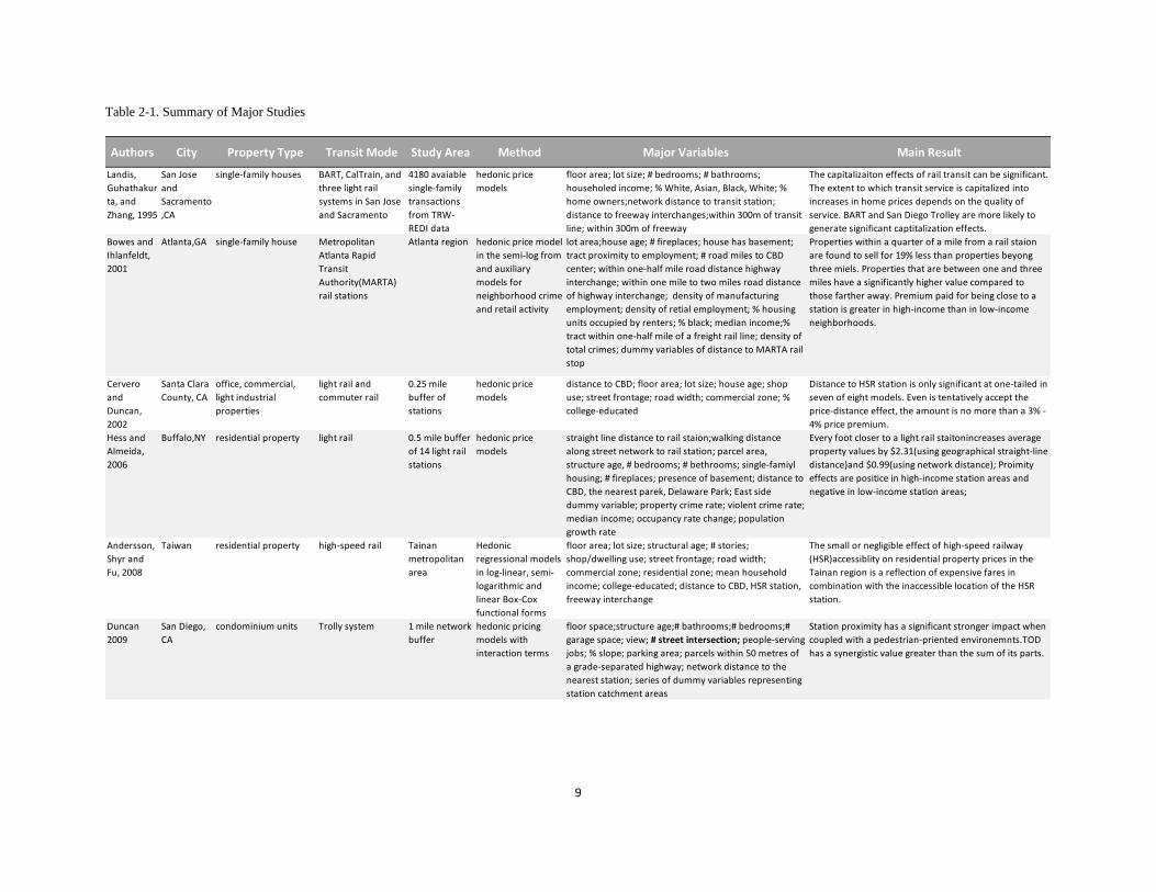
Detailed information of methods, variables, and results are summarized in Table 2-1.
9
Table 2-1. Summary of Major Studies
Authors City Property Type Transit Mode Study Area Method Major Variables Main Result
Landis,
Guhathakur
ta, and
Zhang, 1995
San Jose
and
Sacramento
,CA
single-family houses BART, CalTrain, and
three light rail
systems in San Jose
and Sacramento
4180 avaiable
single-family
transactions
from TRW-
REDI data
hedonic price
models
floor area; lot size; # bedrooms; # bathrooms;
householed income; % White, Asian, Black, White; %
home owners;network distance to transit station;
distance to freeway interchanges;within 300m of transit
line; within 300m of freeway
The capitalizaiton effects of rail transit can be significant.
The extent to which transit service is capitalized into
increases in home prices depends on the quality of
service. BART and San Diego Trolley are more likely to
generate significant captitalization effects.
Bowes and
Ihlanfeldt,
2001
Atlanta,GA single-family house Metropolitan
Atlanta Rapid
Transit
Authority(MARTA)
rail stations
Atlanta region hedonic price model
in the semi-log from
and auxiliary
models for
neighborhood crime
and retail activity
lot area;house age; # fireplaces; house has basement;
tract proximity to employment; # road miles to CBD
center; within one-half mile road distance highway
interchange; within one mile to two miles road distance
of highway interchange; density of manufacturing
employment; density of retial employment; % housing
units occupied by renters; % black; median income;%
tract within one-half mile of a freight rail line; density of
total crimes; dummy variables of distance to MARTA rail
stop
Properties within a quarter of a mile from a rail staion
are found to sell for 19% less than properties beyong
three miels. Properties that are between one and three
miles have a significantly higher value compared to
those farther away. Premium paid for being close to a
station is greater in high-income than in low-income
neighborhoods.
Cervero
and
Duncan,
2002
Santa Clara
County, CA
office, commercial,
light industrial
properties
light rail and
commuter rail
0.25 mile
buffer of
stations
hedonic price
models
distance to CBD; floor area; lot size; house age; shop
use; street frontage; road width; commercial zone; %
college-educated
Distance to HSR station is only significant at one-tailed in
seven of eight models. Even is tentatively accept the
price-distance effect, the amount is no more than a 3% -
4% price premium.
Hess and
Almeida,
2006
Buffalo,NY residential property light rail 0.5 mile buffer
of 14 light rail
stations
hedonic price
models
straight line distance to rail staion;walking distance
along street network to rail station; parcel area,
structure age, # bedrooms; # bethrooms; single-famiyl
housing; # fireplaces; presence of basement; distance to
CBD, the nearest parek, Delaware Park; East side
dummy variable; property crime rate; violent crime rate;
median income; occupancy rate change; population
growth rate
Every foot closer to a light rail staitonincreases average
property values by $2.31(using geographical straight-line
distance)and $0.99(using network distance); Proimity
effects are positice in high-income station areas and
negative in low-income station areas;
Andersson,
Shyr and
Fu, 2008
Taiwan residential property high-speed rail Tainan
metropolitan
area
Hedonic
regressional models
in log-linear, semi-
logarithmic and
linear Box-Cox
functional forms
floor area; lot size; structural age; # stories;
shop/dwelling use; street frontage; road width;
commercial zone; residential zone; mean household
income; college-educated; distance to CBD, HSR station,
freeway interchange
The small or negligible effect of high-speed railway
(HSR)accessiblity on residential property prices in the
Tainan region is a reflection of expensive fares in
combination with the inaccessible location of the HSR
station.
Duncan
2009
San Diego,
CA
condominium units Trolly system 1 mile network
buffer
hedonic pricing
models with
interaction terms
floor space;structure age;# bathrooms;# bedrooms;#
garage space; view; # street intersection; people-serving
jobs; % slope; parking area; parcels within 50 metres of
a grade-separated highway; network distance to the
nearest station; series of dummy variables representing
station catchment areas
Station proximity has a significant stronger impact when
coupled with a pedestrian-priented environemnts.TOD
has a synergistic value greater than the sum of its parts.
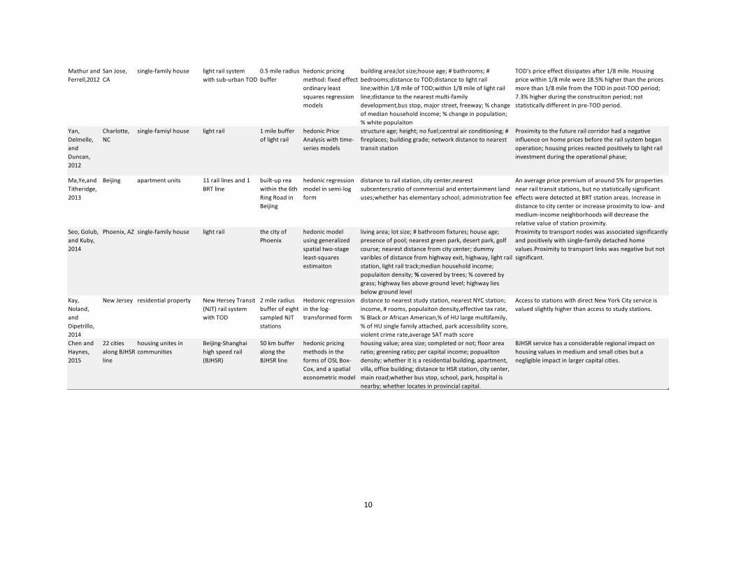
10
Mathur and
Ferrell,2012
San Jose,
CA
single-family house light rail system
with sub-urban TOD
0.5 mile radius
buffer
hedonic pricing
method: fixed effect
ordinary least
squares regression
models
building area;lot size;house age; # bathrooms; #
bedrooms;distance to TOD;distance to light rail
line;within 1/8 mile of TOD;within 1/8 mile of light rail
line;distance to the nearest multi-family
development,bus stop, major street, freeway; % change
of median household income; % change in population;
% white populaiton
TOD's price effect dissipates after 1/8 mile. Housing
price within 1/8 mile were 18.5% higher than the prices
more than 1/8 mile from the TOD in post-TOD period;
7.3% higher during the construciton period; not
statistically different in pre-TOD period.
Yan,
Delmelle,
and
Duncan,
2012
Charlotte,
NC
single-famiyl house light rail 1 mile buffer
of light rail
hedonic Price
Analysis with time-
series models
structure age; height; no fuel;central air conditioning; #
fireplaces; building grade; network distance to nearest
transit station
Proximity to the future rail corridor had a negative
influence on home prices before the rail system began
operation; housing prices reacted positively to light rail
investment during the operational phase;
Ma,Ye,and
Titheridge,
2013
Beijing apartment units 11 rail lines and 1
BRT line
built-up rea
within the 6th
Ring Road in
Beijing
hedonic regression
model in semi-log
form
distance to rail station, city center,nearest
subcenters;ratio of commercial and entertainment land
uses;whether has elementary school; administration fee
An average price premium of around 5% for properties
near rail transit stations, but no statistically significant
effects were detected at BRT station areas. Increase in
distance to city center or increase proximity to low- and
medium-income neighborhoods will decrease the
relative value of station proximity.
Seo, Golub,
and Kuby,
2014
Phoenix, AZ single-family house light rail the city of
Phoenix
hedonic model
using generalized
spatial two-stage
least-squares
estimaiton
living area; lot size; # bathroom fixtures; house age;
presence of pool; nearest green park, desert park, golf
course; nearest distance from city center; dummy
varibles of distance from highway exit, highway, light rail
station, light rail track;median household income;
populaiton density; % covered by trees; % covered by
grass; highway lies above ground level; highway lies
below ground level
Proximity to transport nodes was associated significantly
and positively with single-family detached home
values.Proximity to transport links was negative but not
significant.
Kay,
Noland,
and
Dipetrillo,
2014
New Jersey residential property New Hersey Transit
(NJT) rail system
with TOD
2 mile radius
buffer of eight
sampled NJT
stations
Hedonic regression
in the log-
transformed form
distance to nearest study station, nearest NYC station;
income, # rooms, populaiton density,effective tax rate,
% Black or African American,% of HU large multifamily,
% of HU single family attached, park accessibility score,
violent crime rate,average SAT math score
Access to stations with direct New York City service is
valued slightly higher than access to study stations.
Chen and
Haynes,
2015
22 cities
along BJHSR
line
housing unites in
communities
Beijing-Shanghai
high speed rail
(BJHSR)
50 km buffer
along the
BJHSR line
hedonic pricing
methods in the
forms of OSL Box-
Cox, and a spatial
econometric model
housing value; area size; completed or not; floor area
ratio; greening ratio; per capital income; popualiton
density; whether it is a residential building, apartment,
villa, office building; distance to HSR station, city center,
main road;whether bus stop, school, park, hospital is
nearby; whether locates in provincial capital.
BJHSR service has a considerable regional impact on
housing values in medium and small cities but a
negligible impact in larger capital cities.
11
2.2 Analysis Methods
The term “hedonic modeling” was coined by Court (1939) and popularized by
researchers such as Griliches (1961) and Rosen (1974), whose hedonic price model explained the
composition of housing price by disentangling the bundle of housing services. The concept of
housing as a commonly traded with a specific set of characteristics are widely accepted
(Morancho, 2003) and Hedonic Pricing Analysis (HPA) has been employed to lots of studies
investigating on property values.
Empirical studies typically use sales data of real estate transactions across a wide range of
development conditions to tease out the amount that buyers are willing to pay for the individual
features that make up the total price of a piece of real estate (Dubin, 1998). Marginal price of
each individual feature is estimated in hedonic regression models.
Different functional forms of hedonic regression models are employed in previous
studies. A linear function implies constant marginal implicit prices, which is only tenable under
the situation that constant returns to sale in production or costless repackaging of two or more
bundles (Goodman, 1998). In non-linear function forms, the price of an additional unit of an
attribute depends on the quantity already supplied and in the most common specifications also on
the quantity of other attributes (Andersson, Shyr and Fu, 2008). It is examined that some
structural and neighborhood factors have non-linear relations with housing price, such as interior
square footage. Many other studies shows that non-linear functions are more suitable when
applied to typical housing markets. Seo, Golub, and Kuby (2014) tested linear, semi-logarithmic,
and trans-logarithmic functional forms in their study of Phoenix light rail system. Chen and
Haynes (2015) made use of a robust ordinary least square regression, a Box-Cox transformed
12
maximum likelihood form, and a spatial econometric modeling form to demonstrate robustness
of estimations. Model results might vary with different regression forms. “The log-linear
function explains more of the variance and has greater log likelihood. All the Box-Cox functions
have slightly greater log likelihood than the log-linear function with the exception of the simple
left-hand side model” (Andersson, Shyr and Fu, 2008).
Many studies conducted time-series models to analysis the impacts of different
construction periods. Ferguson (1988) examined the relationship between urban transit and
single family housing prices in Vancouver and his work shows that the urban transit has an
impact on housing market before the system operations began. Mathur and Ferrell (2012)
estimated models in pre-TOD construction period, TOD construction period, and post-TOD
construction period. They found TOD’s price effects are significantly positive in the construction
and post-construction periods. Similarly, Pan (2013) made an analysis of light-rail in Houston
and indicated that there is a significant increase in property values following the announcement
that the light-rail line would be constructed. However, Yan, Delmelle, and Duncan (2012)
identified four time periods of pre-planning, planning, construction, and operation phase of light
rail system. Their results suggest that proximity to the future rail corridor has a negative
influence on housing price in the first three periods.
Geographical extent of the market is one major issue concerned by hedonic price
functions. Empirical studies demonstrate that if the assumed market is larger than its real size, it
leads to biased parameter coefficients; if the assumed size is smaller, it leads to parameter
estimates with lower precision (Palmquist, 1991). In the case of impacts from TOD or rail
services, many studies indicates that the impact is within a certain proximity, roughly from a
quarter mile to two miles. According to Goodman and Thibodeau (1998), limiting the study
13
area’s spatial extent has the benefit of making it more homogeneous, which simplifies the model
specification and is likely to lead to a more accurate model. Most previous researches focus on
buffer areas around transit stations using a radial distance up to one mile around stations (Hess
and Almeida, 2006).
According to Bartholomew and Ewing (2011), HPA is classified as one of several
revealed-preference (RP) approaches for determining public goods value, which makes use of
empirical data to determine people’s willingness to pay. HPA has the intuitive strength of being
able to demonstrate what people actually choose when they are required to prioritize competing
demands for time and money. On the contrary, it shares the same limitations with RP
approaches. One fundamental one is its inability to test demands for goods that do not yet exist,
because the analysis is based on observed available data. Another common issue with hedonic
real estate models is spatial dependence, which implies spatial correlation among observations in
cross-sectional data that are assumed to be independent (Anselin 1988; Kim et al., 2003). To
obtain unbiased, consistent, and efficient estimates, spatial dependences should be tested and
addressed with proper methods if either one or both spatial effects exist
14
CHAPTER 3 METHODOLOGY
This study seeks to estimate the capitalization of light rail transit-oriented development
(TOD) on residential properties. While a number of previous studies investigate TOD impacts by
its component characteristics, the study aims to capture its integrated influence.
3.1 Question and Hypothesis
Research question can be stated as: How do light rail TOD impact residential property
values? In order to answer this question, two dimensions are given emphasis to explore,
including: the different impact caused by the difference in residential properties; the different
impact caused by different time periods. Generally speaking, I suppose as TOD accessibility
increases, residential property values increases; impact of TOD are different across pre-
construction, during-construction, and after-construction periods. Comparisons among different
residential properties and across time periods can be conducted.
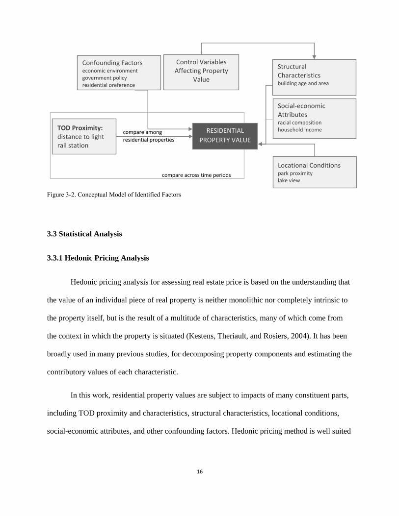
3.2 Conceptual Model
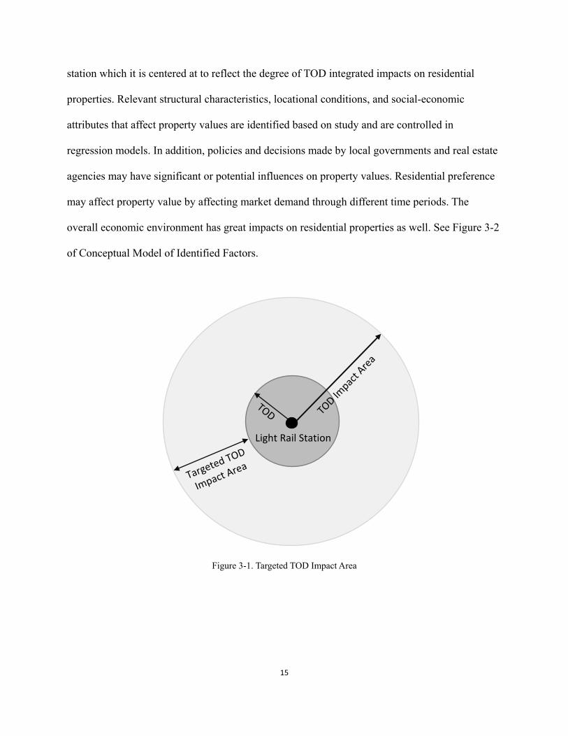
Normally, TOD is centered at a light rail station. TOD impacts cover both the areas within
its boundaries that apply specific policies and designations, and the areas adjacent to it. To analyze
the integrated effects of TOD component characteristics, the study considers TOD applied areas
as a whole and differentiate it from TOD impact areas. Therefore, residential properties within
TOD boundaries are not considered. See Figure 3-1 of Targeted TOD Impact Area.
Under the consideration of data availability, residential property values are represented by
single-family house values in the study. TOD proximity is measured as distance to the light rail
15
station which it is centered at to reflect the degree of TOD integrated impacts on residential
properties. Relevant structural characteristics, locational conditions, and social-economic
attributes that affect property values are identified based on study and are controlled in
regression models. In addition, policies and decisions made by local governments and real estate
agencies may have significant or potential influences on property values. Residential preference
may affect property value by affecting market demand through different time periods. The
overall economic environment has great impacts on residential properties as well. See Figure 3-2
of Conceptual Model of Identified Factors.
Figure 3-1. Targeted TOD Impact Area
Light Rail Station
16
Figure 3-2. Conceptual Model of Identified Factors
3.3 Statistical Analysis
3.3.1 Hedonic Pricing Analysis
Hedonic pricing analysis for assessing real estate price is based on the understanding that
the value of an individual piece of real property is neither monolithic nor completely intrinsic to
the property itself, but is the result of a multitude of characteristics, many of which come from
the context in which the property is situated (Kestens, Theriault, and Rosiers, 2004). It has been
broadly used in many previous studies, for decomposing property components and estimating the
contributory values of each characteristic.
In this work, residential property values are subject to impacts of many constituent parts,
including TOD proximity and characteristics, structural characteristics, locational conditions,
social-economic attributes, and other confounding factors. Hedonic pricing method is well suited
TOD Proximity: distance to light rail station
Structural Characteristics building age and area
Locational Conditions park proximity lake view
Social-economic Attributes racial composition household income
Confounding Factors economic environment government policy residential preference
Control Variables Affecting Property
Value
RESIDENTIAL
PROPERTY VALUE compare among
residential properties
compare across time periods
17
to separate impacts from all related factors and examine the relations between each of them with
residential property values. The study applies hedonic regression models in linear form:
P = c0 +∑αi Ti + ∑βi Li +∑μi Si +∑υi Ei + ε
Where c0 is a constant, P is the adjusted transaction price of single family property, Ti are the
TOD proximity variable; Li are the other identified locational variables; Si are structural
variables; Ei are related social-economic variables, ε is the regression residual.
3.3.2 Regression Models
To analyze TOD impacts of different time periods, pre-during-after models are conducted
in the basic form of hedonic regression function. Residential properties’ transaction year are
identified and classified into three categories: before TOD construction, during TOD
construction, and after TOD construction. Comparisons among different properties and across
different time periods are then conducted.
18
Chapter 4 Study Area
4.1 Link Light Rail
Link Light Rail is a rapid transit rail system in the Seattle metropolitan area of
Washington State. It was first proposed and approved in 1996, in response to population growth
and urban development. The original designation involves two rail lines, Tacoma Link and
Central Link, which were shortened afterwards due to financial and political difficulties. In 2003,
Tacoma Link light rail line opened, consisting of six stops and 1.6 miles through downtown
Tacoma. Then the construction of Central Link light rail line began. By the late 2009, the
construction was completed and opened to the public, running between Westlake station and
Seattle-Tacoma international Airport. In 2016, Central Link was further extended by adding two
more stations, Capitol Hill station and University of Washington station. Sound Transit is the
region’s mass transportation agency that take charge of the designation, construction, and
operation of Link Light Rail. It has made further plans to extend Link Light Rail to Lynnwood
Transit Center to the north, and Downtown Bellevue and Overlake Transit Center to the east.
Currently, the Central Link light rail travels 18.8 miles between UW station and Seattle-
Tacoma international Airport. It consists of 13 stops along the way and runs at 6, 10 or 15
minutes intervals depending on the time of day.
4.2 Station Area Overlay District
Before the construction of Central Link light rail, the City of Seattle started a program of
Station Area Planning in 1998. In partnership with Sound Transit, Station Area Planning
19
engaged city departments, community representatives, and partner agencies in planning and
development work for a quarter mile around proposed light rail stations. The program refined the
community’s vision, identified public and private investments, and made specific policy choices
and designations to guide future development of the station areas. In 2000, the Seattle City
Council adopted 10 Station Area Concept-Level Recommendation packages. In 2001, the
Council further passed the Station Area Overlay legislation.
Station Area Overlay legislation establishes Station Area Overlay Districts (SAOD) and
rezones around eight future light rail stations. The primary goal of the legislation is to promote
Transit-Oriented Development (TOD) and forward neighborhood goals for walkable town
centers. Specific policies are applied to SAODs: supporting existing business by allowing for a
one-time expansion of certain existing business; providing off-site residential parking by leasing
parking on nearby site; prohibiting specific uses such as vehicle repair and warehouse;
promoting flexibility in commercial zones by allowing Single-Purpose Residential (SPR) use;
encouraging more housing development by removing 64% upper level coverage limits, in which
case residential buildings in commercial zones of SAODs can use the entire lot area on all levels
for residential units. Zoning changes are made primarily within SAOD boundaries. For most
cases, zoning changes provide greater design flexibility by removing height and density limits
for residential uses, promoting more retail and commercial uses in residential and commercial
zones, and reinforce pedestrian activities by adding pedestrian overlay designation along the
main corridors. The above policies and designations synergistically facilitate TOD by promoting
high-density and mixed-use development, and prevent auto-oriented development in SAOD.
20
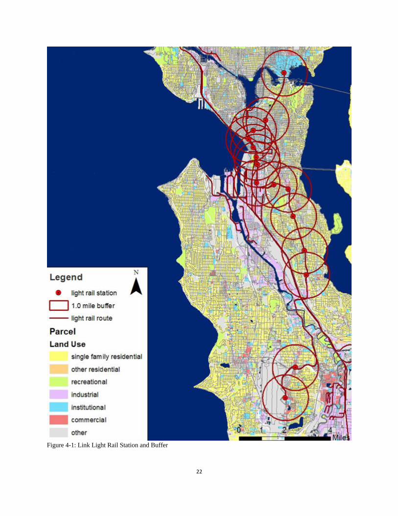
4.3 Study Area Selection and Description
In order to analysis the impact of light rail TOD on residential property values, the study
areas should satisfy the following criteria: TOD should be around light rail stations; land-value
benefits from TOD take time to accrue, so the operation of light rail stations should be long
enough, in this study, more than five years; the study area should contain a certain number of
single-family houses, before and after TOD implementation; the study area should not overlap
with TOD, in order to analysis the integrated impact of TOD.
Therefore, Station Area Overlay Districts, which are established around light rail stations
and promote TOD, are reviewed for study area selection. Considering of the distance between
each two light rail stations, buffers are created within 1.0 mile radius of station. Suitable study
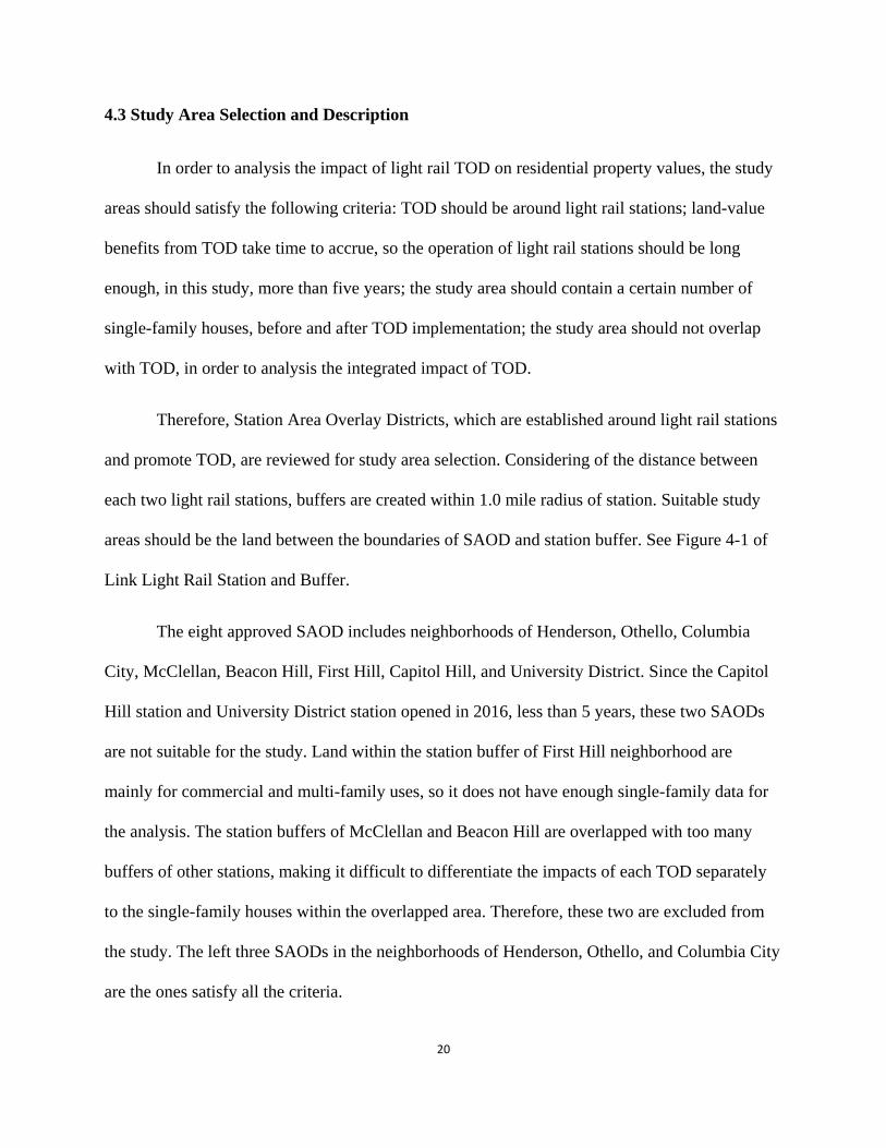
areas should be the land between the boundaries of SAOD and station buffer. See Figure 4-1 of
Link Light Rail Station and Buffer.
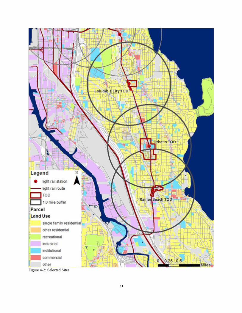
The eight approved SAOD includes neighborhoods of Henderson, Othello, Columbia
City, McClellan, Beacon Hill, First Hill, Capitol Hill, and University District. Since the Capitol
Hill station and University District station opened in 2016, less than 5 years, these two SAODs
are not suitable for the study. Land within the station buffer of First Hill neighborhood are
mainly for commercial and multi-family uses, so it does not have enough single-family data for
the analysis. The station buffers of McClellan and Beacon Hill are overlapped with too many
buffers of other stations, making it difficult to differentiate the impacts of each TOD separately
to the single-family houses within the overlapped area. Therefore, these two are excluded from
the study. The left three SAODs in the neighborhoods of Henderson, Othello, and Columbia City
are the ones satisfy all the criteria.
21
Therefore, suitable study areas are the areas between the boundaries of 1.0 mile radius
from Rainer Beach, Othello, and Columbia City stations and SAODs of Henderson, Othello, and
Columbia City neighborhoods. To be simplified, study areas are referred as Rainer Beach site,
Othello site, and Columbia City site. The borders of the three SAODs are represented for the
TOD borders of Rainer Beach site, Othello site, and Columbia City site, and they are referred as
Rainer Beach TOD, Othello TOD, and Columbia City TOD in the study. See Figure 4-2 of
Selected Sites.
After the Station Area Overlay legislation was approved, a number of actions were
implemented to promote Transit-Oriented Development. The Seattle Housing Authority (SHA)
built approximately 1400 mixed-income rental and ownership units adjacent to the Othello
Station. The construction is completed in 2005. For other two study sites, the new constructions
and adjustments took place gradually from 2001. All TOD components in the three sites
completed before the light rail stations went in service in 2009. Therefore, the TOD timeline is
divided into three periods: 1996–2001period before the construction of TOD and station; 2002–
2009 period during the constructions; 2010–2016 after TOD construction completed and stations
went into service.
22
Figure 4-1: Link Light Rail Station and Buffer
23
Figure 4-2: Selected Sites
Columbia City TOD
Othello TOD
Rainer Beach TOD
24
Chapter 5 Data
5.1 Data Source
King County GIS Center contains geospatial databases of administrative, environmental,
transportation, recreation and property information. Three study sites and the major features in
the area are established making use of these databases. Parcel data included in the property
database provides locational and identification information of single family houses. Present use
of each parcel is also included, which is used to identify different kinds of land uses.
King County Assessor provides parcel, residential building, and real property sales
database. Some physical and structural characteristics of single family houses are extracted from
parcel and residential building database. Transaction data and sale price information are stored in
the real property sales database. Attributes of “major” and “minor” are used to generate “pin
code” to link with geospatial parcels.
United States Census offers American Community Survey (ACS) data providing facts of
people, housing, and business at the block-group level. Block-group shape-file is available for
identifying parcels of different block groups. Attribute of “GEOID” is used to link the
information to geospatial parcels.
City of Seattle Legislative Information Service provides detailed information of council
bills and ordinances. The ordinances relating to designate boundaries for the Station Area
Overlay District are recorded on the website. Maps of Station Area Overlay District Boundaries
for Link light rail stations are available to acquire.

25
S&P/Case-Shiller Home Price Index Series measures changes in the total value of all
existing single-family housing stock. It provides home price index of Seattle, measuring the
average change in value of residential real estate in Seattle given a constant level of quality from
1990 till now. Index of different years is used for inflating the previous housing prices into
present dollars, in order to capture the effect of economic change (especially the Subprime Crisis
in U.S. during 2007-2009) on real estate market.
5.2 Parcel Extraction
Three study areas between TOD boundary and 1.0 mile buffer around each Link light rail
station are established using ArcMap, including Columbia City site, Othello site, and Rainer
Beach site. Some areas within the three sites are overlapped with each other. For parcels in those
areas, calculate their distance to stations and distribute the parcels to the nearest one: if the parcel
is closer to Othello station, it is counted as a parcel of Othello site in the regression models. For
this purpose, buffer around Mt. Baker station is used to eliminate parcels in Columbia City
buffer that are closer to Mt. Baker station. Therefore, all the parcels are distributed to the three
study sites according to their distances to stations.
Qualified parcels are identified through four steps:
1) Parcels should be of single family uses. The attribute of present use from parcel data shows
the land use classifications. Values equal to 2, 6, and 9, indicating single family uses in
residential use/zone and C/I zone. Parcels with other values are excluded. There are 12217
satisfied parcels in total, out of which 5216 are in Columbia City site, 4351 are in Othello
site, and 2650 are in Rainer Beach site. See Figure 5-1of Properties by Study Sites.
26
2) Parcels should have only one living unit. Residential building table from King County
Assessor records the number of living unit for each parcel. Since the study targets on single
family properties, parcels with more than one living unit number are eliminated. 671
parcels do not meet the requirement and are removed.
3) Parcels characteristics should keep consistent as they were sold. Transaction date is
recorded in the attribute of document year from real property sales table, and renovation
year is recorded in residential building table. Link these two tables and compare the value
of them. Since only current conditions of parcels are reflected, single family houses whose
transaction date smaller than renovation date are excluded.
4) Parcels attributes’ values should all be available and reasonable. Database from other
resources are linked with geospatial parcel shape file in ArcMap. Some of the parcels that
could not be matched with recorded data are eliminated. Some of the parcels whose added
attributes values are obviously unreasonable are removed.
In summary, there are 3443 qualified parcel records, out of which 1436 belongs to Columbia
City site, 1207 belongs to Othello site, and 800 belongs to Rainer Beach site. If classified by time
periods, there are 519 records for pre-construction period, 2486 for during-construction period,
and 438 for after-construction period. See table 5-1 of Qualified Parcel Records.
27
Figure 5-1. Properties by Study Sites
28
Table 5-1: Qualified Parcel Records
Period Station
pre-construction period
(1996-2001)
during-construction period
(2002-2009)
after-construction period
(2010-2016)
Total
Rainer Beach station 112 569 119 800
Othello station 170 876 161 1207
237 1041 158 1436
Total 519 2486 438 3443
5.3 Variables
5.3.1 Explanatory TOD Variables
Integrated impact of TOD components is represented by TOD proximity, which is
measured by distance from residential properties to the nearest light rail station. Instead of using
continuous distance variable, the study sets binary distance bands as 0-0.25 mile, 0.25-0.50 mile,
0.50-0.75 mile, and 0.75-1 mile to light rail station and applies these dummy variables in
regression models. These variables are calculated by using spatial analysis tool in ArcMap.
5.3.2 Control Variables
Social-economic attributes of single family houses are extracted from related survey
results in U.S. Census and calculated in ArcMap. Since the information is generated in block-
group level “GEOID” attribute and block-group data are used to attach the information to each
parcel. ArcGIS tools of spatial join, calculate geometry are used to calculate percentage of white,
as an indicator of race composition. Other social-economic factors include median household
income. Social-economic attributes are generated in block group level.
Columbia City station
29
Locational conditions of single family houses are extracted from parcel table in King
County Assessor and measured using spatial analysis tool in ArcMap. Lake Washington view is
measured by dummy variables, with value “0” indicating no lake view and value “1” indicating
some level of lake view. Traffic noise is measured in this way too. These two factors are linked
with single family houses by “pin code” attribute in ArcMap.
Major features in the study area are generated in ArcMap, including transport network,
recreational facilities, and natural resources. Distance from each parcel to the nearest park,
nearest commercial land use, freeway, and lake Washington are calculated. Network analysis is
used for generate intersections from transport networks, in order to calculate number of
intersections in block group level.
Structural characteristics are extracted from residential building table and parcel table of
King County Assessor, including building grade, condition, bedrooms number, total finished
area above grade, total basement area, and lot size. Attributes of document year from sale price
table and built year from residential building table are used to calculate building age.
5.3.3 Dependent Variable
Transaction prices of single family houses are recorded in real property sales table from
King County Assessor. S&P/Case-Shiller Home Price Index data for Seattle from 1996 to 2016
is extracted to inflating previous price to present dollars of 2016.
The computational formula is:
Vn = Vp×(Hn /Hp)
30
Where Vn is the value of dollar in present year; Vp is the dollar value in past year; Hn is the Home
Price Index in present year; Hp is the Home Price Index in past year.
The adjusted transaction price is applied to regression models as the dependent variable.
5.3.4 Variable Definitions and Sources
All of the above variables are applied to regression models. See Table 5-2 of Variable
Definitions and Data Sources.
Table 5-2 Variable Definitions and Data Sources
VARIABLE DEFINITION MAJOR SOURCES
DEPENDENT VARIABLE VN single family house transaction price
adjusted to 2016 constant dollars King County Assessor real property sales data S&P/Case-Shiller Home Price Index Series
EXPLANATORY TOD VARIABLES
D_DUMMY1 1, if property is located within 0.25 mile distance from light rail station, 0 otherwise
King County GIS shape file, City of Seattle Legislative Information Service
D_DUMMY2 1, if property is located within 0.25-0.5 mile distance from light rail station, 0 otherwise
King County GIS shape file, City of Seattle Legislative Information Service
D_DUMMY3 1, if property is located within 0.5-0.75 mile distance from light rail station, 0 otherwise
King County GIS shape file, City of Seattle Legislative Information Service
LOCATIONAL VARIABLE
D_PARK distance to nearest park King County recreation shape file
D_COMUSE distance to nearest commercial land uses King County administrative and parcel shape file
31
D_LAKE distance to lake Washington King County environmental shape file
D_FREEWAY distance to freeway King County transportation shape file
INTERSECTIONS number of intersections in block group level
King County transportation shape file, U.S. Census block group data
TRANOISE 1, if the property has detected traffic noise, 0 otherwise
King County Assessor parcel data
LAKVIEW 1, if the property has other nuisance, 0 otherwise
King County Assessor parcel data
SOCIAL-ECONOMIC VARIABLE
P_WHITE percentage of white population summarized to the block level
American Community Survey 5-year (2010-2014) B02001 Data
M_INCOME median household income in block-group level
American Community Survey 5-year (2010-2014) B19013 Data
STRUCTURAL VARIABLE BEDROOMS number of bedrooms King County Assessor residential
building data
AGE building age King County Assessor residential building and real property sales data
LOT SIZE square footage of lot King County Assessor parcel data
TOTFINISHED square footage of total finished area above grade of the building
King County Assessor residential building data
TOTBASEMENT square footage of total basement of the building
King County Assessor residential building data
CONDITION the score representing the condition of the building from low to high: 1 poor, 2 fair, 3 average, 4 good, 5 very good; 0 otherwise
King County Assessor residential building data
BUIGRADE the score representing the building quality from low to high:1 cabin, 2 substandard, 3 poor, 4 low, 5 fair, 6 low average, 7 average, 8 good, 9 better, 10 very good, 11 excellent, 12 luxury, 13 mansion
King County Assessor residential building data
32
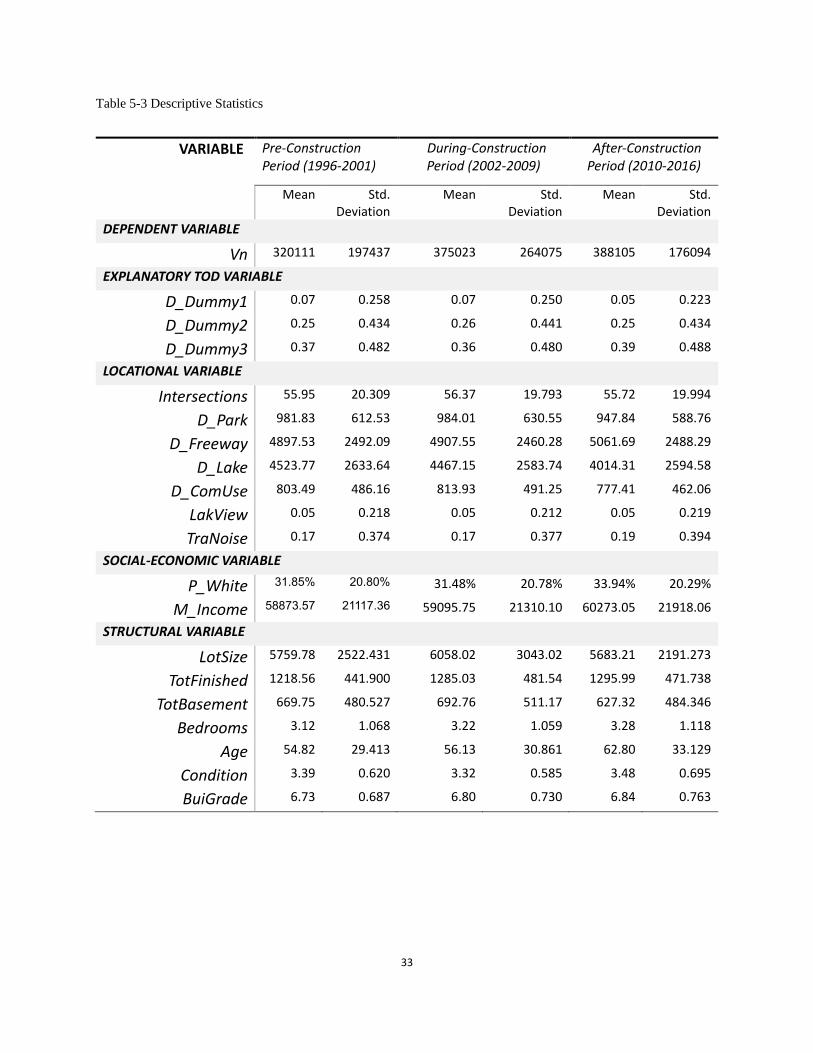
5.4 Descriptive Statistics
The flowing descriptive statistics table summarize the mean and standard deviation of
each variable for all three sites models of pre-during-after construction periods.
The average inflated single family house price increases from pre-construction period to
after-construction period. The price fluctuation is most obvious during the construction time,
indicating the unstable market environment at that time. The mean and standard deviation of
distance dummy variables across the three periods are similar.
In terms of locational factors, the mean and standard deviation of most variables do not
change much across pre-during-after construction periods. The mean distance to nearest park is
around 980 feet for pre and during construction periods, while it decreases slightly after TOD
construction completed. The mean distance to commercial land uses decreases as TOD
construction completed, while the mean traffic noise level increases in the after-construction
period. For social-economic factors, percentage of white increases slightly when TOD
construction completed. Median household income increase gradually across the three periods
from $58873.57 to $60273.05. As for structural factors, some of their mean values increases in
during-construction periods and decreases when the construction was completed, such as lot size
and total basement area. The condition and building grade of properties increase across time
periods. Square footage of total finished area above grade of the building increases stably from
1218.56 to 1295.99 square feet from pre-construction to after-construction period.
33
Table 5-3 Descriptive Statistics
VARIABLE Pre-Construction Period (1996-2001)
During-Construction Period (2002-2009)
After-Construction Period (2010-2016)
Mean Std. Deviation
Mean Std. Deviation
Mean Std. Deviation
DEPENDENT VARIABLE
Vn 320111 197437 375023 264075 388105 176094
EXPLANATORY TOD VARIABLE
D_Dummy1 0.07 0.258 0.07 0.250 0.05 0.223
D_Dummy2 0.25 0.434 0.26 0.441 0.25 0.434
D_Dummy3 0.37 0.482 0.36 0.480 0.39 0.488
LOCATIONAL VARIABLE
Intersections 55.95 20.309 56.37 19.793 55.72 19.994
D_Park 981.83 612.53 984.01 630.55 947.84 588.76
D_Freeway 4897.53 2492.09 4907.55 2460.28 5061.69 2488.29
D_Lake 4523.77 2633.64 4467.15 2583.74 4014.31 2594.58
D_ComUse 803.49 486.16 813.93 491.25 777.41 462.06
LakView 0.05 0.218 0.05 0.212 0.05 0.219
TraNoise 0.17 0.374 0.17 0.377 0.19 0.394
SOCIAL-ECONOMIC VARIABLE
P_White 31.85% 20.80% 31.48% 20.78% 33.94% 20.29%
M_Income 58873.57 21117.36 59095.75 21310.10 60273.05 21918.06
STRUCTURAL VARIABLE
LotSize 5759.78 2522.431 6058.02 3043.02 5683.21 2191.273
TotFinished 1218.56 441.900 1285.03 481.54 1295.99 471.738
TotBasement 669.75 480.527 692.76 511.17 627.32 484.346
Bedrooms 3.12 1.068 3.22 1.059 3.28 1.118
Age 54.82 29.413 56.13 30.861 62.80 33.129
Condition 3.39 0.620 3.32 0.585 3.48 0.695
BuiGrade 6.73 0.687 6.80 0.730 6.84 0.763
34
CHAPTER 6 MODEL RESULTS
Regression models are conducted for properties of the three sites in pre-during-after
construction periods. Comparisons among different properties and across time periods are
conducted.
In the study, linear functional forms are employed in regression models. Pearson
correlation values are tested to examine if there are multi-collinearity problems among selected
variables. Variance inflation factor (VIF) is examined to quantify the severity of multi-
collinearity. Some variables are dropped or their measurements are adjusted if they are correlated
with each other. The F test results suggest that housing price could be explained as the integrated
influences of identified variables. The adjusted R square is examined to see the proportions of
variations in housing price explained by the variations of identified variables. Coefficients and
significance level of each variable are demonstrated and discussed as the following.
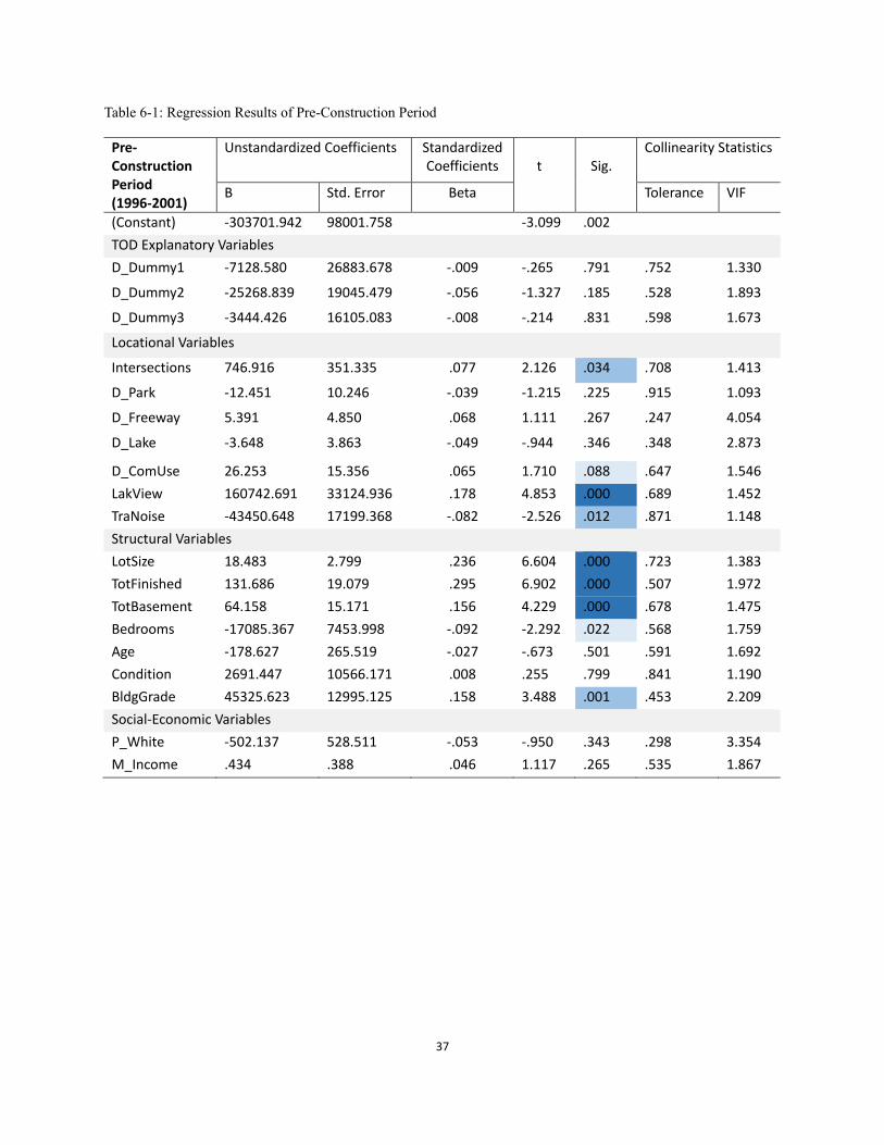
6.1 Pre-Construction Period
Pre-construction period is from 1996 to 2001. There are totally 519 valid data applied to
pre-construction period model. The adjusted R square shows that the model can explain 52.1%
variations in housing price. VIF of variables shows there is no serious multi-collinearity
problems.
Using distance band of 0.75-1 mile from station as reference group, distance dummy
variables have no statistical significance influence on housing price, but it demonstrates a decline
tendency for properties located within 0.25 miles to station and an increase tendency for
properties located farther. Mean price of properties located within 0.5-0.75 miles might be about
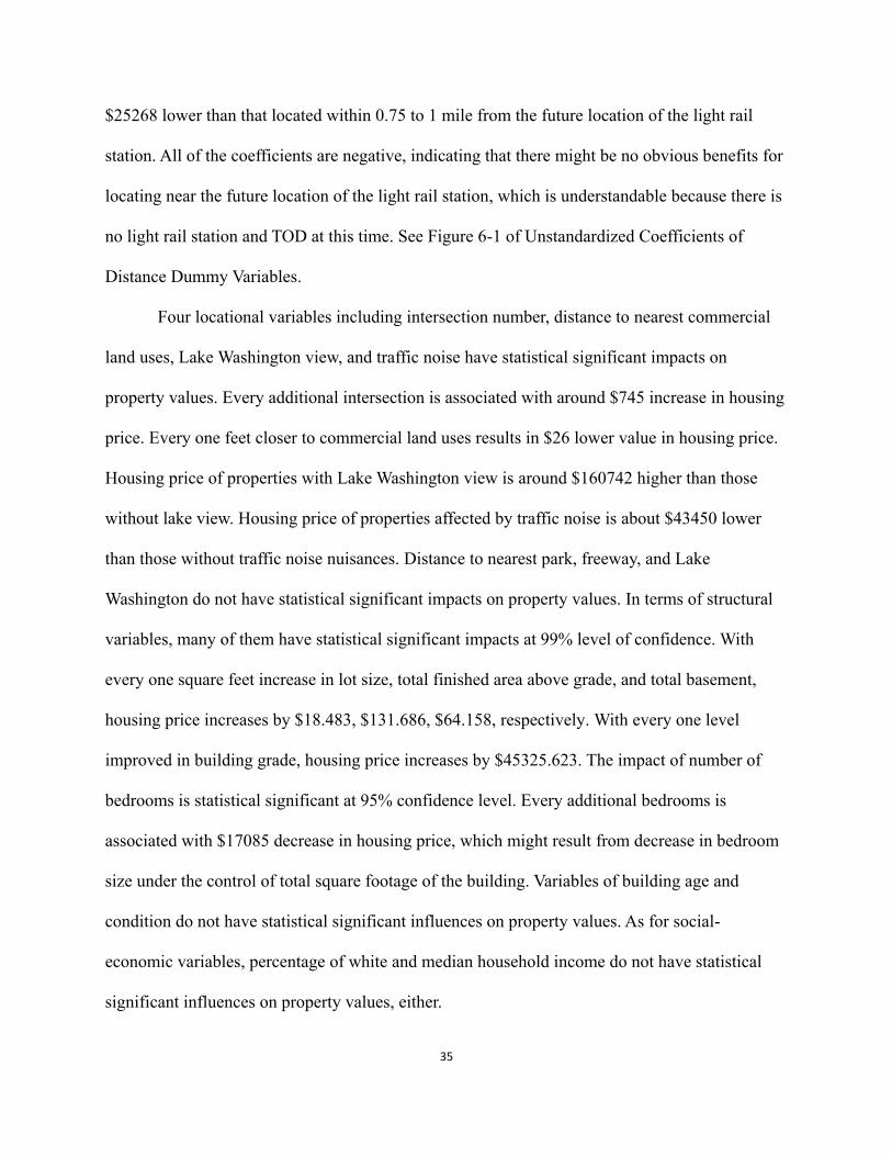
35
$25268 lower than that located within 0.75 to 1 mile from the future location of the light rail
station. All of the coefficients are negative, indicating that there might be no obvious benefits for
locating near the future location of the light rail station, which is understandable because there is
no light rail station and TOD at this time. See Figure 6-1 of Unstandardized Coefficients of
Distance Dummy Variables.
Four locational variables including intersection number, distance to nearest commercial
land uses, Lake Washington view, and traffic noise have statistical significant impacts on
property values. Every additional intersection is associated with around $745 increase in housing
price. Every one feet closer to commercial land uses results in $26 lower value in housing price.
Housing price of properties with Lake Washington view is around $160742 higher than those
without lake view. Housing price of properties affected by traffic noise is about $43450 lower
than those without traffic noise nuisances. Distance to nearest park, freeway, and Lake
Washington do not have statistical significant impacts on property values. In terms of structural
variables, many of them have statistical significant impacts at 99% level of confidence. With
every one square feet increase in lot size, total finished area above grade, and total basement,
housing price increases by $18.483, $131.686, $64.158, respectively. With every one level
improved in building grade, housing price increases by $45325.623. The impact of number of
bedrooms is statistical significant at 95% confidence level. Every additional bedrooms is
associated with $17085 decrease in housing price, which might result from decrease in bedroom
size under the control of total square footage of the building. Variables of building age and
condition do not have statistical significant influences on property values. As for social-
economic variables, percentage of white and median household income do not have statistical
significant influences on property values, either.
36
Comparison of standardized coefficients reflects the different influences of identified
variables to housing price. The most influential variables are structural variables, including lot
size and total finished area above grade. See Table 6-1 of Regression Results of Pre-Construction
Period.
Figure 6-1: Unstandardized Coefficients of Dummy Variables for Before-Construction Periods
37
Table 6-1: Regression Results of Pre-Construction Period
Pre-Construction Period (1996-2001)
Unstandardized Coefficients Standardized Coefficients
t
Sig.
Collinearity Statistics
B Std. Error Beta Tolerance VIF
(Constant) -303701.942 98001.758 -3.099 .002
TOD Explanatory Variables
D_Dummy1 -7128.580 26883.678 -.009 -.265 .791 .752 1.330
D_Dummy2 -25268.839 19045.479 -.056 -1.327 .185 .528 1.893
D_Dummy3 -3444.426 16105.083 -.008 -.214 .831 .598 1.673
Locational Variables
Intersections 746.916 351.335 .077 2.126 .034 .708 1.413
D_Park -12.451 10.246 -.039 -1.215 .225 .915 1.093
D_Freeway 5.391 4.850 .068 1.111 .267 .247 4.054
D_Lake -3.648 3.863 -.049 -.944 .346 .348 2.873
D_ComUse 26.253 15.356 .065 1.710 .088 .647 1.546
LakView 160742.691 33124.936 .178 4.853 .000 .689 1.452
TraNoise -43450.648 17199.368 -.082 -2.526 .012 .871 1.148
Structural Variables
LotSize 18.483 2.799 .236 6.604 .000 .723 1.383
TotFinished 131.686 19.079 .295 6.902 .000 .507 1.972
TotBasement 64.158 15.171 .156 4.229 .000 .678 1.475
Bedrooms -17085.367 7453.998 -.092 -2.292 .022 .568 1.759
Age -178.627 265.519 -.027 -.673 .501 .591 1.692
Condition 2691.447 10566.171 .008 .255 .799 .841 1.190
BldgGrade 45325.623 12995.125 .158 3.488 .001 .453 2.209
Social-Economic Variables
P_White -502.137 528.511 -.053 -.950 .343 .298 3.354
M_Income .434 .388 .046 1.117 .265 .535 1.867
38
6.2 During-Construction Period
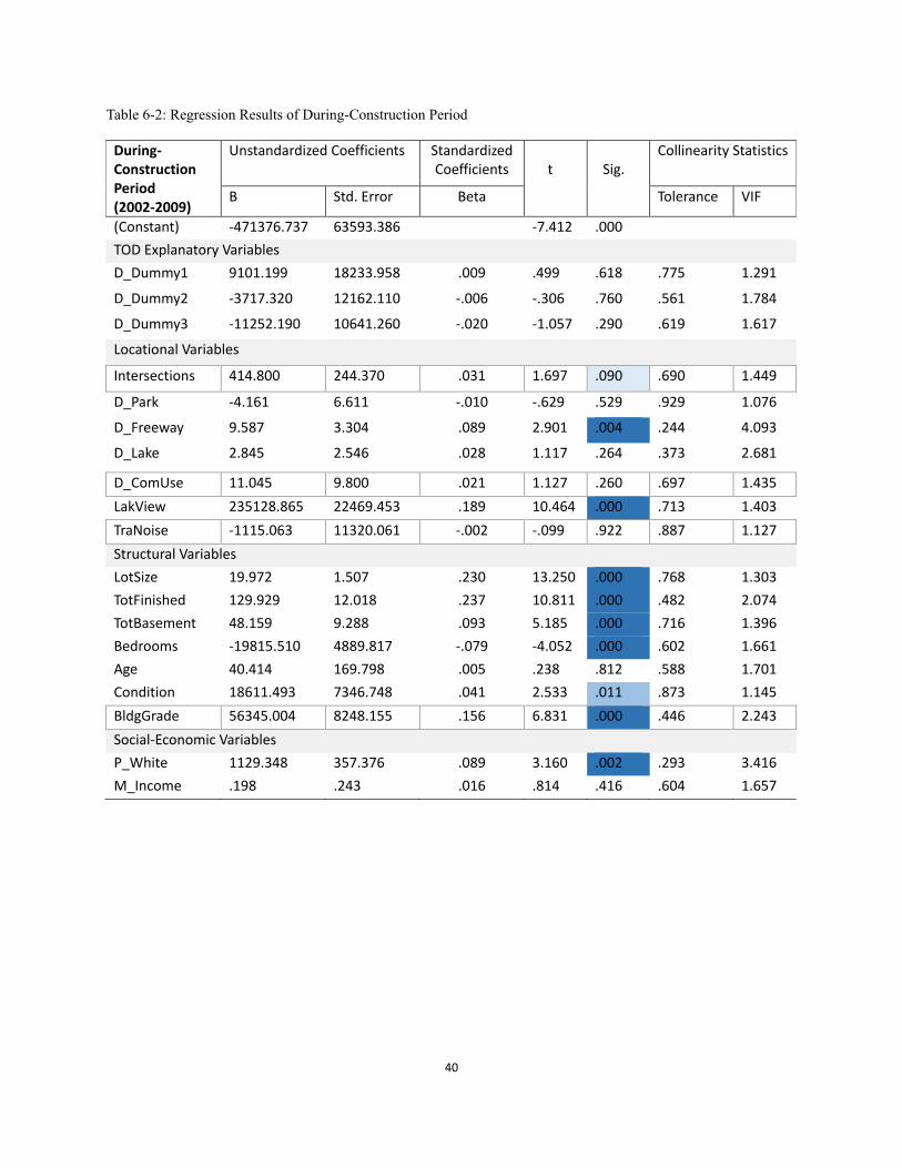
During-construction period is from 2002 to 2009. There are totally 2486 valid data
applied to during-construction period model. The adjusted R square shows that the model can
explain 42.5% variations in housing price. VIF of variables shows there is no serious multi-
collinearity problems.
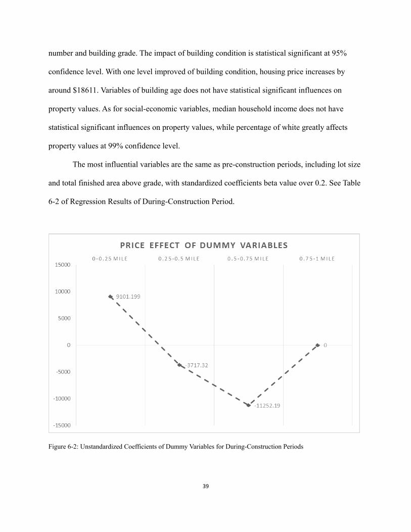
Using distance band of 0.75-1 mile from station as reference group, distance dummy
variables have no statistical significance influence on housing price, but it demonstrates a decline
tendency for properties located within 0.50 miles to station and an increase tendency for
properties located farther. Mean price of properties located within 0.25 miles might be about
$9101.199 higher compared with properties located in 0.75-1 mile distance band, indicating that
the construction of TOD might generate premiums of properties right adjacent to it. Mean price
of properties located within 0.25-0.75 miles and 0.5-0.75 miles might be about $3717.32 and
$11252.19 lower. See Figure 6-2 of Unstandardized Coefficients of Dummy Variables for
During-Construction Periods.
Three locational variables including intersection number, distance to freeway, and Lake
Washington view have statistical significant impacts on property values. Every additional
intersection is associated with around $414.8 increase in housing price. Every one feet closer to
freeway results in $9.587 lower value in housing price. Housing price of properties with Lake
Washington view is around $235128 higher than those without lake view. Distance to nearest
park, commercial land uses, and Lake Washington do not have statistical significant impacts on
property values. The impact of traffic noise is not statistical significant at this time. In terms of
structural variables, most of them have statistical significant impacts at 99% level of confidence,
including lot size, total square footage of finished area above grade, total basement, bedrooms
39
number and building grade. The impact of building condition is statistical significant at 95%
confidence level. With one level improved of building condition, housing price increases by
around $18611. Variables of building age does not have statistical significant influences on
property values. As for social-economic variables, median household income does not have
statistical significant influences on property values, while percentage of white greatly affects
property values at 99% confidence level.
The most influential variables are the same as pre-construction periods, including lot size
and total finished area above grade, with standardized coefficients beta value over 0.2. See Table
6-2 of Regression Results of During-Construction Period.
Figure 6-2: Unstandardized Coefficients of Dummy Variables for During-Construction Periods
40
Table 6-2: Regression Results of During-Construction Period
During-Construction Period (2002-2009)
Unstandardized Coefficients Standardized Coefficients
t
Sig.
Collinearity Statistics
B Std. Error Beta Tolerance VIF
(Constant) -471376.737 63593.386 -7.412 .000
TOD Explanatory Variables
D_Dummy1 9101.199 18233.958 .009 .499 .618 .775 1.291
D_Dummy2 -3717.320 12162.110 -.006 -.306 .760 .561 1.784
D_Dummy3 -11252.190 10641.260 -.020 -1.057 .290 .619 1.617
Locational Variables
Intersections 414.800 244.370 .031 1.697 .090 .690 1.449
D_Park -4.161 6.611 -.010 -.629 .529 .929 1.076
D_Freeway 9.587 3.304 .089 2.901 .004 .244 4.093
D_Lake 2.845 2.546 .028 1.117 .264 .373 2.681
D_ComUse 11.045 9.800 .021 1.127 .260 .697 1.435
LakView 235128.865 22469.453 .189 10.464 .000 .713 1.403
TraNoise -1115.063 11320.061 -.002 -.099 .922 .887 1.127
Structural Variables
LotSize 19.972 1.507 .230 13.250 .000 .768 1.303
TotFinished 129.929 12.018 .237 10.811 .000 .482 2.074
TotBasement 48.159 9.288 .093 5.185 .000 .716 1.396
Bedrooms -19815.510 4889.817 -.079 -4.052 .000 .602 1.661
Age 40.414 169.798 .005 .238 .812 .588 1.701
Condition 18611.493 7346.748 .041 2.533 .011 .873 1.145
BldgGrade 56345.004 8248.155 .156 6.831 .000 .446 2.243
Social-Economic Variables
P_White 1129.348 357.376 .089 3.160 .002 .293 3.416
M_Income .198 .243 .016 .814 .416 .604 1.657
41
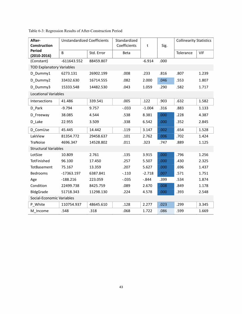
6.3 After-Construction Period
After-construction period is from 2010 to 2016. There are totally 438 valid data applied
to after-construction period model. The adjusted R square shows that the model can explain
58.9% variations in housing price. VIF of variables shows there is no serious multi-collinearity
problems.
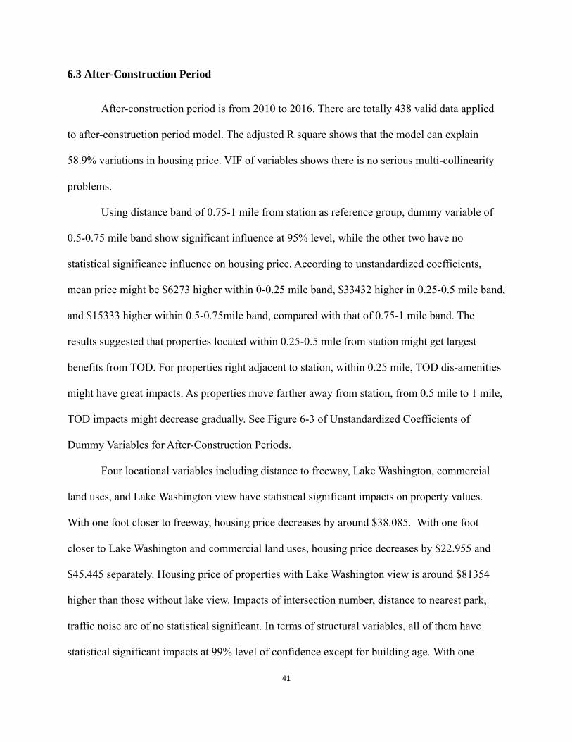
Using distance band of 0.75-1 mile from station as reference group, dummy variable of
0.5-0.75 mile band show significant influence at 95% level, while the other two have no
statistical significance influence on housing price. According to unstandardized coefficients,
mean price might be $6273 higher within 0-0.25 mile band, $33432 higher in 0.25-0.5 mile band,
and $15333 higher within 0.5-0.75mile band, compared with that of 0.75-1 mile band. The
results suggested that properties located within 0.25-0.5 mile from station might get largest
benefits from TOD. For properties right adjacent to station, within 0.25 mile, TOD dis-amenities
might have great impacts. As properties move farther away from station, from 0.5 mile to 1 mile,
TOD impacts might decrease gradually. See Figure 6-3 of Unstandardized Coefficients of
Dummy Variables for After-Construction Periods.
Four locational variables including distance to freeway, Lake Washington, commercial
land uses, and Lake Washington view have statistical significant impacts on property values.
With one foot closer to freeway, housing price decreases by around $38.085. With one foot
closer to Lake Washington and commercial land uses, housing price decreases by $22.955 and
$45.445 separately. Housing price of properties with Lake Washington view is around $81354
higher than those without lake view. Impacts of intersection number, distance to nearest park,
traffic noise are of no statistical significant. In terms of structural variables, all of them have
statistical significant impacts at 99% level of confidence except for building age. With one
42
square foot increase of lot size, total finished area above grade, and total basement area, housing
price increases by around $10. 81, $96.1, $75.1, respectively. Similar to previous two periods,
bedrooms number has a negative impact on housing price. Condition and building grade have
significant influences on property values: with one level improved, housing price increases by
around $22499 and $51718. Social-economic variables have statistic significant influences on
property values at 90% confidence level. Different from previous two periods, the most
influential variables are locational variables of distance to freeway and Lake Washington. See
Table 6-3 of Regression Results of After-Construction Period.
Figure 6-3: Unstandardized Coefficients of Dummy Variables for After-Construction Periods
43
Table 6-3: Regression Results of After-Construction Period
After-Construction Period (2010-2016)
Unstandardized Coefficients Standardized Coefficients
t
Sig.
Collinearity Statistics
B Std. Error Beta Tolerance VIF
(Constant) -611643.552 88459.807 -6.914 .000
TOD Explanatory Variables
D_Dummy1 6273.131 26902.199 .008 .233 .816 .807 1.239
D_Dummy2 33432.630 16714.555 .082 2.000 .046 .553 1.807
D_Dummy3 15333.548 14482.530 .043 1.059 .290 .582 1.717
Locational Variables
Intersections 41.486 339.541 .005 .122 .903 .632 1.582
D_Park -9.794 9.757 -.033 -1.004 .316 .883 1.133
D_Freeway 38.085 4.544 .538 8.381 .000 .228 4.387
D_Lake 22.955 3.509 .338 6.542 .000 .352 2.845
D_ComUse 45.445 14.442 .119 3.147 .002 .654 1.528
LakView 81354.772 29458.637 .101 2.762 .006 .702 1.424
TraNoise 4696.347 14528.802 .011 .323 .747 .889 1.125
Structural Variables
LotSize 10.809 2.761 .135 3.915 .000 .796 1.256
TotFinished 96.100 17.450 .257 5.507 .000 .430 2.325
TotBasement 75.167 13.359 .207 5.627 .000 .696 1.437
Bedrooms -17363.197 6387.841 -.110 -2.718 .007 .571 1.751
Age -188.216 223.059 -.035 -.844 .399 .534 1.874
Condition 22499.738 8425.759 .089 2.670 .008 .849 1.178
BldgGrade 51718.343 11298.130 .224 4.578 .000 .393 2.548
Social-Economic Variables
P_White 110754.937 48645.610 .128 2.277 .023 .299 3.345
M_Income .548 .318 .068 1.722 .086 .599 1.669
44
CHAPTER 7 CONCLUSION
The study seeks to investigate the impact of transit-oriented development (TOD) on
residential property values using the case of Link light rail TOD in Seattle. Different from
previous studies, which decompose TOD impact into constituent parts, the study captures the
integrated influence and analyzes price effects in pre-during-after construction periods.
Hedonic pricing method is employed to analysis relations between identified variables.
Single-family housing price is studied for representing residential property value. TOD
proximity is measured as dummy variables, which are applied as major independent variables.
Relevant structural characteristics, locational conditions, and social-economic attributes are
identified and controlled in regression models.
Model results suggest that TOD has significant positive impacts on values of residential
properties that are located within 0.25-0.50 mile from the station after construction completed. In
addition, regression outcomes are different across time periods. In pre-construction period, it
indicates that housing price might increase first and then decrease as distance to the location of
future station increases, but the relationships are not statistically significant; in during-
construction period, similar to pre-construction period, TOD impacts are not statistical
significant, but residential properties located within 0.25 mile might benefit from TOD
construction to some degree: mean value of housing price might be around $9000 higher than
that of properties located within 0.75-1 mile from the station. In after-construction period, TOD
has significant positive impacts on values of residential properties located within 0.25-0.50 mile
from the station: mean value of housing price is $33432 higher than that of properties located
within 0.75-1 mile from the station. For properties located less than 0.5 mile but more than 0.25
45
mile (and hence reasonably distant from conceivable negative effects of rail transit, such as noise
and intrusion of strangers), housing price might increase as TOD proximity increases; for
properties located further than 0.5 mile, housing price might decrease as TOD proximity
decreases.
There are some limitations in the study. First, the study does not take control of factors
affecting housing price comprehensively. This is partially due to limitation in data accessibility.
Locational conditions are calculated based on current situations instead of situations at the
transaction time. Social-economic characteristics are extracted from American Community
Survey 5-year (2010-2014) data rather than data of transaction time. This may result in
inaccuracy reflection of actual situation. In addition, it is hard to consider and include all factors
affecting housing price, and some of the missing variables, such as school quality and crime rate,
might be important. Secondly, the study uses Link light rail TOD in Seattle as a case study to
capture the integrated impacts of TOD. Since the implement of Station Area Overlay legislation
and construction of TOD are based on actual situation of Seattle, the results of the study might
not be applicable to TOD in other places with other transit types.
While the study makes use of all three selected sites to analysis the integrated impacts of
TOD on residential properties, further studies could explore more on individual TOD impact on
each site. TOD characteristics could be quantified and price effects could be compared among
different TODs to investigate the internal mechanism, which would be beneficial to future policy
making in relation to TOD programs.

46
Bibliography
Anselin, L. (1988). Lagrange multiplier test diagnostics for spatial dependence and spatial
heterogeneity. Geographical analysis, 20(1), 1-17.
Acharya, G., & Bennett, L. L. (2001). Valuing open space and land-use patterns in urban
watersheds. The Journal of Real Estate Finance and Economics, 22(2-3), 221-237.
Arrington, G. B. (2005, July). TOD in the United States: The experience with light rail.
In Transit-Oriented Development–Making it Happen Conference, Fremantle,
Australia (pp. 5-8).
Anderson, S. T., & West, S. E. (2006). Open space, residential property values, and spatial
context. Regional Science and Urban Economics, 36(6), 773-789.
Atkinson-Palombo, C. (2010). Comparing the capitalisation benefits of light-rail transit and
overlay zoning for single-family houses and condos by neighbourhood type in
metropolitan Phoenix, Arizona. Urban Studies.
Andersson, D. E., Shyr, O. F., & Fu, J. (2010). Does high-speed rail accessibility influence
residential property prices? Hedonic estimates from southern Taiwan. Journal of
Transport Geography, 18(1), 166-174.
Black, A. (1993). The recent popularity of light rail transit in North America. Journal of
Planning Education and Research, 12(2), 150-159.
Bowes, D. R., & Ihlanfeldt, K. R. (2001). Identifying the impacts of rail transit stations on
residential property values. Journal of Urban Economics, 50(1), 1-25.
47
Bae, C. H. C., Jun, M. J., & Park, H. (2003). The impact of Seoul's subway Line 5 on residential
property values. Transport policy, 10(2), 85-94.
Bartholomew, K., & Ewing, R. (2011). Hedonic price effects of pedestrian-and transit-oriented
development. Journal of Planning Literature, 26(1), 18-34.
Cervero, R., & Duncan, M. (2002). Transit's value-added effects: Light and commuter rail
services and commercial land values. Transportation Research Record: Journal of the
Transportation Research Board, (1805), 8-15.
Dubin, R. A. (1998). Spatial autocorrelation: a primer. Journal of housing economics, 7(4), 304-
327.
Debrezion, G., Pels, E., & Rietveld, P. (2007). The impact of railway stations on residential and
commercial property value: a meta-analysis. The Journal of Real Estate Finance and
Economics, 35(2), 161-180.
Dittmar, H., & Ohland, G. (Eds.). (2012). The new transit town: best practices in transit-oriented
development. Island Press.
Hughes, W. T., & Sirmans, C. F. (1992). TRAFFIC EXTERNALITIES AND SINGLE‐
FAMILY HOUSE PRICES*. Journal of Regional Science, 32(4), 487-500.
Hess, D. B., & Almeida, T. M. (2007). Impact of proximity to light rail rapid transit on station-
area property values in Buffalo, New York. Urban studies, 44(5-6), 1041-1068.
Griliches, Z. (1961). Hedonic price indexes for automobiles: An econometric of quality change.
In The Price Statistics of the Federal Goverment (pp. 173-196). NBER.
48
Goodman, A. C. (1998). Andrew Court and the invention of hedonic price analysis. Journal of
urban economics, 44(2), 291-298.
Goodman, A. C., & Thibodeau, T. G. (1998). Housing market segmentation. Journal of housing
economics, 7(2), 121-143.
Kim, C. W., Phipps, T. T., & Anselin, L. (2003). Measuring the benefits of air quality
improvement: a spatial hedonic approach. Journal of environmental economics and
management, 45(1), 24-39.
Kestens, Y., Theriault, M., & Des Rosiers, F. (2004). The impact of surrounding land use and
vegetation on single-family house prices.Environment and Planning B: Planning and
Design, 31(4), 539-567.
Kay, A. I., Noland, R. B., & DiPetrillo, S. (2014). Residential property valuations near transit
stations with transit-oriented development. Journal of Transport Geography, 39, 131-
140.
Landis, J., Guhathakurta, S., Huang, W., Zhang, M., & Fukuji, B. (1995). Rail transit
investments, real estate values, and land use change: a comparative analysis of five
California rail transit systems.
Lutzenhiser, M., & Netusil, N. R. (2001). The effect of open spaces on a home's sale
price. Contemporary Economic Policy, 19(3), 291-298.
Matthews, J. W., & Turnbull, G. K. (2007). Neighborhood street layout and property value: The
interaction of accessibility and land use mix. The journal of real estate finance and
economics, 35(2), 111-141.
49
Morancho, A. B. (2003). A hedonic valuation of urban green areas. Landscape and urban
planning, 66(1), 35-41.
Mathur, S. (2008). Impact of transportation and other jurisdictional-level infrastructure and
services on housing prices. Journal of Urban Planning and Development, 134(1), 32-41.
Mathur, S., & Ferrell, C. (2009). Effect of suburban transit oriented developments on residential
property values.
Mathur, S., & Ferrell, C. (2013). Measuring the impact of sub-urban transit-oriented
developments on single-family home values. Transportation Research Part A: Policy and
Practice, 47, 42-55.
Ma, L., Ye, R., & Titheridge, H. (2013). Capitalization effects of rail transit and BRT on
residential property values in a booming economy: evidence from Beijing. In the13th
World Conference on Transportation Research, Rio de Janeiro, Brazil, July.
Pucher, J., & Renne, J. L. (2003). Socioeconomics of urban travel: evidence from the 2001
NHTS. Transportation Quarterly, 57(3), 49-77.
Pan, Q. (2013). The impacts of an urban light rail system on residential property values: a case
study of the Houston METRO Rail transit line. Transportation Planning and
Technology, 36(2), 145-169.
Rosen, S. (1974). Hedonic prices and implicit markets: product differentiation in pure
competition. Journal of political economy, 82(1), 34-55.
Rajamani, J., Bhat, C., Handy, S., Knaap, G., & Song, Y. (2003). Assessing impact of urban
form measures on non-work trip mode choice after controlling for demographic and
50
level-of-service effects. Transportation Research Record: Journal of the Transportation
Research Board, (1831), 158-165.
Smith, V. K., Palmquist, R. B., & Jakus, P. (1991). Combining Farrell frontier and hedonic travel
cost models for valuing estuarine quality. The Review of Economics and Statistics, 694-
699.
Strand, J., & Vågnes, M. (2001). The relationship between property values and railroad
proximity: a study based on hedonic prices and real estate brokers'
appraisals. Transportation, 28(2), 137-156.
Seo, K., Golub, A., & Kuby, M. (2014). Combined impacts of highways and light rail transit on
residential property values: a spatial hedonic price model for Phoenix, Arizona. Journal
of Transport Geography, 41, 53-62.
Recommended