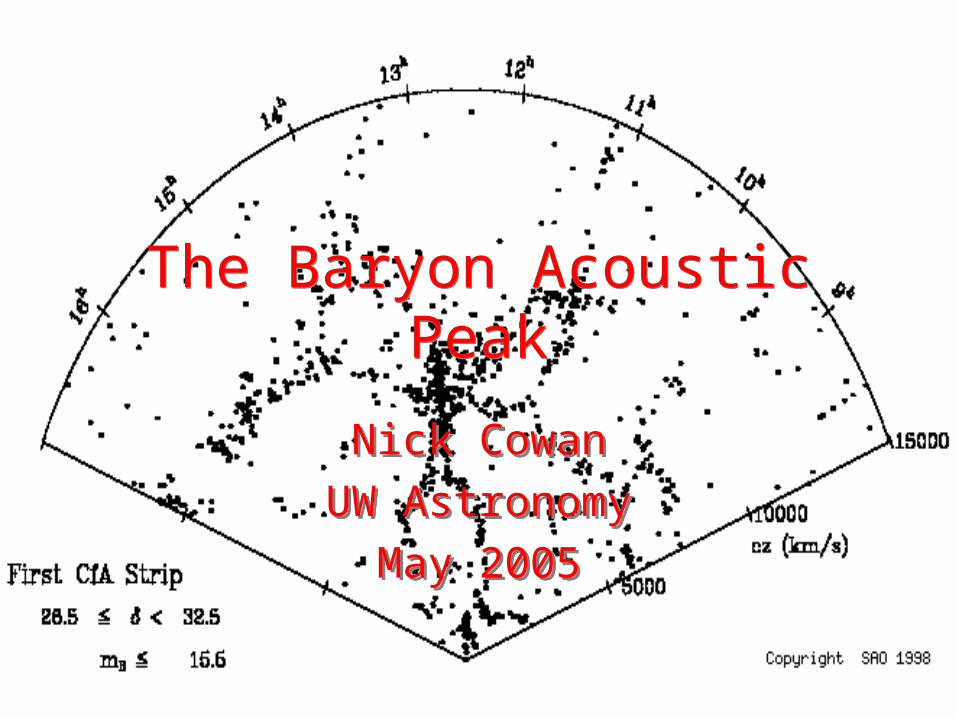
The Baryon Acoustic PeakThe Baryon Acoustic Peak
Nick Cowan
UW Astronomy
May 2005
Nick Cowan
UW Astronomy
May 2005
Outline
• Acoustic Peak• Statistical Methods• Results from SDSS• Summary
QuickTime™ and aTIFF (Uncompressed) decompressor
are needed to see this picture.
Acoustic Peak
• Quantum fluctuations led to density variations in the early universe.
• These density fluctuations generated sound waves.
• Those sounds waves are responsible for the large-scale structure of the universe.
QuickTime™ and aTIFF (Uncompressed) decompressor
are needed to see this picture.
Density Fluctuations
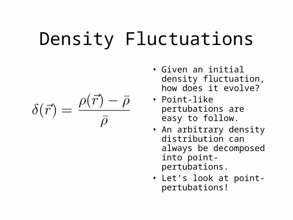
• Given an initial density fluctuation, how does it evolve?
• Point-like pertubations are easy to follow.
• An arbitrary density distribution can always be decomposed into point-pertubations.
• Let’s look at point-pertubations!
Point-like Pertubation
QuickTime™ and aTIFF (Uncompressed) decompressor
are needed to see this picture.
(comoving)
(r2)
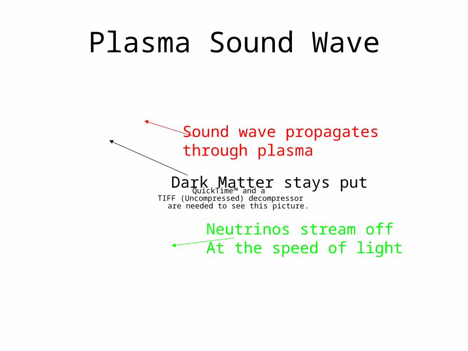
Plasma Sound Wave
QuickTime™ and aTIFF (Uncompressed) decompressor
are needed to see this picture.
Neutrinos stream offAt the speed of light
Dark Matter stays put
Sound wave propagates through plasma
Perturbation at Decoupling
QuickTime™ and aTIFF (Uncompressed) decompressor
are needed to see this picture.
Photons Break Free
QuickTime™ and aTIFF (Uncompressed) decompressor
are needed to see this picture.
Photons streamoff at speed of light
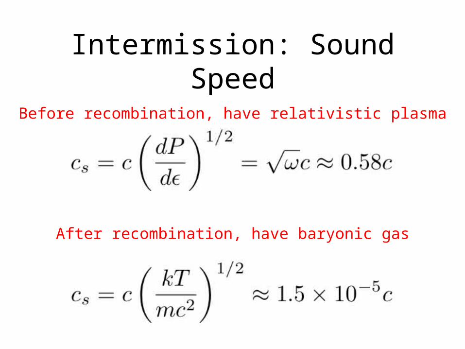
Intermission: Sound Speed
Before recombination, have relativistic plasma
After recombination, have baryonic gas
Sound Wave Stalls
QuickTime™ and aTIFF (Uncompressed) decompressor
are needed to see this picture.
Dark Matter and Baryons Flirt
QuickTime™ and aTIFF (Uncompressed) decompressor
are needed to see this picture.
Baryons fall back intocentral potential DM falls
into shell
Dark Matter and Baryons Merge
QuickTime™ and aTIFF (Uncompressed) decompressor
are needed to see this picture.
Nowadays we expect baryons and DMto track each other.
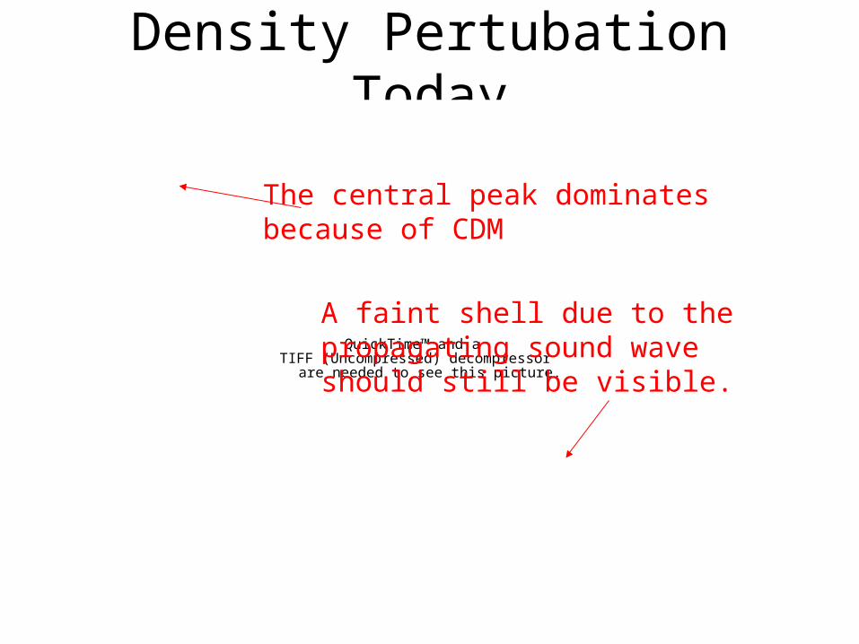
Density Pertubation Today
QuickTime™ and aTIFF (Uncompressed) decompressor
are needed to see this picture.
The central peak dominatesbecause of CDM
A faint shell due to the propagating sound waveshould still be visible.
Statistical Methods
• The specific density distribution of our universe is hard to obtain and contains loads of useless information.
• The statistics of galaxy distribution should contain all the useful information.
QuickTime™ and aTIFF (Uncompressed) decompressor
are needed to see this picture.
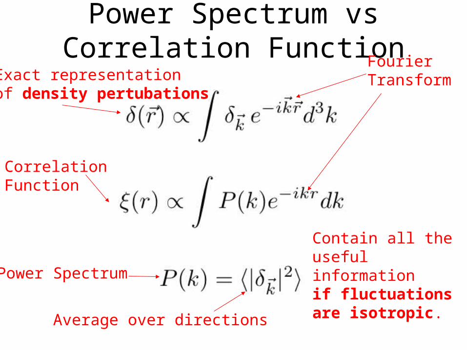
Power Spectrum vs Correlation Function
Fourier Transform
Power Spectrum
Contain all the useful information if fluctuations are isotropic.
Correlation Function
Average over directions
Exact representation of density pertubations
2-point Correlation Function
QuickTime™ and aTIFF (Uncompressed) decompressor
are needed to see this picture.QuickTime™ and a
TIFF (Uncompressed) decompressorare needed to see this picture.
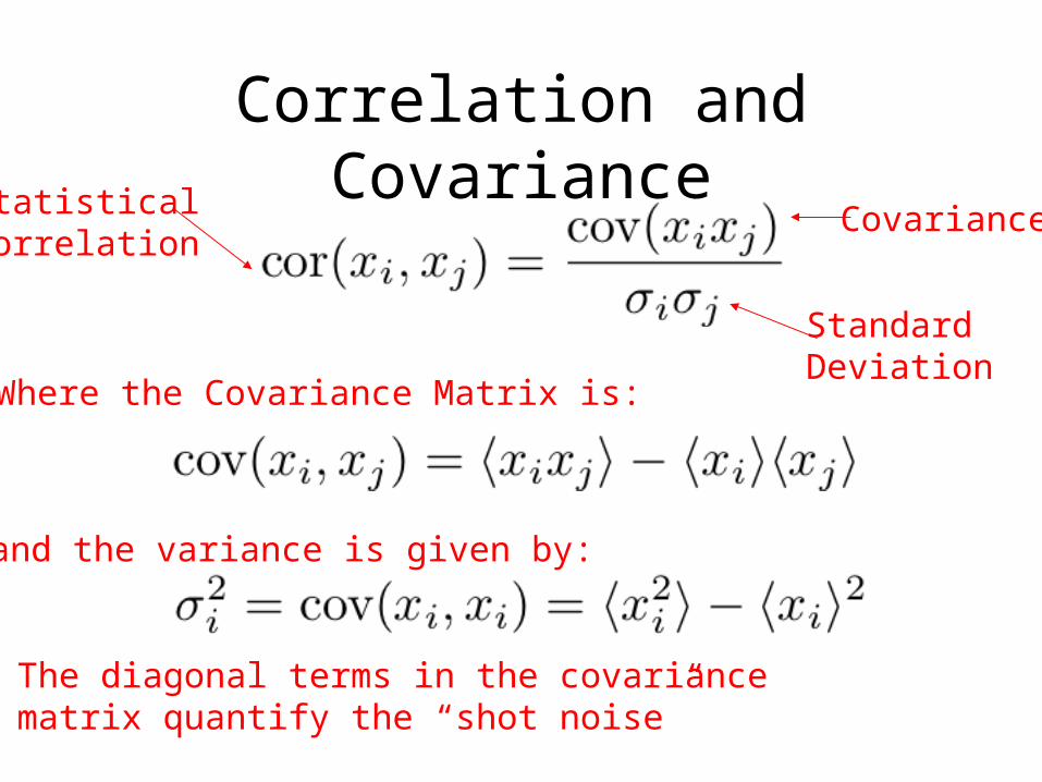
Correlation and CovarianceStatistical Correlation
Covariance
Where the Covariance Matrix is:
and the variance is given by:
The diagonal terms in the covariance matrix quantify the “shot noise”
StandardDeviation
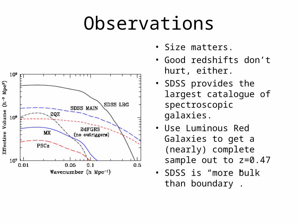
Observations• Size matters.• Good redshifts don’t
hurt, either.• SDSS provides the
largest catalogue of spectroscopic galaxies.
• Use Luminous Red Galaxies to get a (nearly) complete sample out to z=0.47
• SDSS is “more bulk than boundary”.
Flashback
QuickTime™ and aTIFF (Uncompressed) decompressor
are needed to see this picture.
The central peak dominatesbecause of CDM
A faint shell due to the propagating sound waveshould still be visible.
Correlation Function
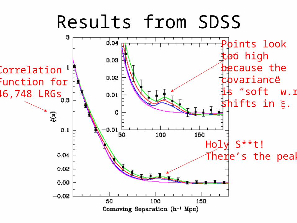
Results from SDSS
CorrelationFunction for46,748 LRGs
Points looktoo highbecause the covariance is “soft” w.r.t.shifts in .
Holy S**t!There’s the peak!
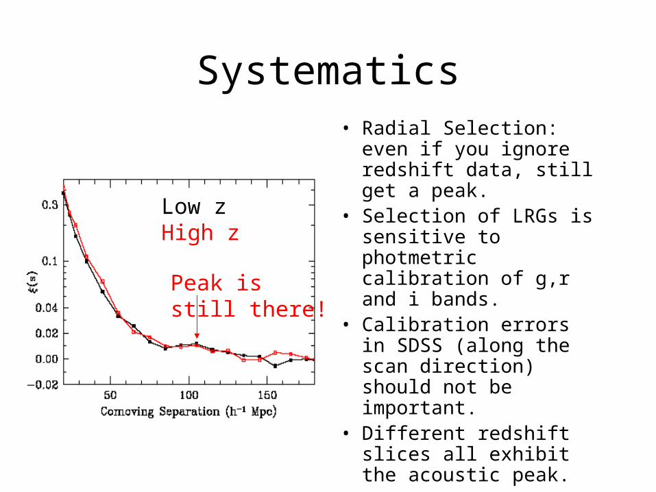
Systematics• Radial Selection: even if
you ignore redshift data, still get a peak.
• Selection of LRGs is sensitive to photmetric calibration of g,r and i bands.
• Calibration errors in SDSS (along the scan direction) should not be important.
• Different redshift slices all exhibit the acoustic peak.
Low zHigh z
Peak is still there!
Covariance Matrix• The covariance matrix is constructed from the
sample of LRGs.• It shows considerable correlation between
neighboring bins (off-diagonal terms) and an enhanced diagonal from shot noise.
2 = 16.1/17 which is reasonable.• Check the matrix by comparing jack-knifed
samples to each other. • Compare to a covariance matrix based on the
Gaussian approximation.• Other fancy statistical tricks
Summary
• Sound waves stall at recombination.• They should always be found the same
distance from the central CDM peak.• We can still see the signature of these
sound waves in the distribution of galaxies as a baryon acoustic peak.
• The position and size of the peak is consistent with the WMAP cosmology.
References
• Eisenstein et al, astro-ph/0501171
• Eisenstein, “What is the Acoustic Peak?”
• Peacock, Cosmological Physics (1999)
• Ryden, Introduction to Cosmology (2003)
Recommended