arX
iv:a
stro
-ph/
0609
417v
1 1
4 S
ep 2
006
Tests of general relativity from timing the doublepulsar
M. Kramer,1∗ I.H. Stairs,2 R.N. Manchester,3 M.A. McLaughlin,1,4
A.G. Lyne,1 R.D. Ferdman,2 M. Burgay,5 D.R. Lorimer,1,4
A. Possenti,5 N. D’Amico,5,6 J.M. Sarkissian,3 G.B. Hobbs,3
J.E. Reynolds,3 P.C.C. Freire7 and F. Camilo8
1University of Manchester, Jodrell Bank Observatory, Macclesfield, SK11 9DL, UK2Dept. of Physics and Astronomy, University of British Columbia, 6224 Agricultural Road,
Vancouver, BC V6T 1Z1, Canada3Australia Telescope National Facility, CSIRO, P.O. Box 76,Epping NSW 1710, Australia
4Department of Physics, West Virginia University, Morgantown, WV 26505, USA5INAF - Osservatorio Astronomica di Cagliari, Loc. Poggio dei Pini, Strada 54,
09012 Capoterra, Italy6Universita’ degli Studi di Cagliari, Dipartimento di Fisica, SP Monserrato-Sestu km 0.7,
09042 Monserrato (CA), Italy7NAIC, Arecibo Observatory, HC03 Box 53995, PR 00612, USA
8Columbia Astrophysics Laboratory, Columbia University, 550 West 120th Street,
New York, NY 10027, USA
∗To whom correspondence should be addressed; E-mail: [email protected]
The double pulsar system, PSR J0737-3039A/B, is unique in that both neutron
stars are detectable as radio pulsars. This, combined with significantly higher
mean orbital velocities and accelerations when compared toother binary pul-
sars, suggested that the system would become the best available testbed for
general relativity and alternative theories of gravity in the strong-field regime.
1

Here we report on precision timing observations taken over the 2.5 years since
its discovery and present four independent strong-field tests of general rela-
tivity. Use of the theory-independent mass ratio of the two stars makes these
tests uniquely different from earlier studies. By measuring relativistic correc-
tions to the Keplerian discription of the orbital motion, we find that the “post-
Keplerian” parameter s agrees with the value predicted by Einstein’s theory
of general relativity within an uncertainty of 0.05%, the most precise test yet
obtained. We also show that the transverse velocity of the system’s center of
mass is extremely small. Combined with the system’s location near the Sun,
this result suggests that future tests of gravitational theories with the double
pulsar will supersede the best current Solar-system tests.It also implies that
the second-born pulsar may have formed differently to the usually assumed
core-collapse of a helium star.
Introduction. Einstein’s general theory of relativity (GR) has so far passed all experimental
tests with flying colours (1), with the most precise tests achieved in the weak-field gravity
conditions of the Solar System (2, 3). However, it is conceivable that GR breaks down under
extreme conditions such as strong gravitational fields where other theories of gravity may apply
(4). Predictions of gravitational radiation and self-gravitational effects can only be tested using
massive and compact astronomical objects such as neutron stars and black holes. Studies of
the double-neutron-star binary systems, PSR B1913+16 and PSR B1534+12, have provided the
best such tests so far, confirming GR at the 0.2% and 0.7% level, respectively (5, 6) 1. The
recently discovered double pulsar system, PSR J0737-3039A/B, has significantly higher mean1Stairs et al. (2002, ref. (6)) find an agreement of their measured values for PSR B1534+12with GR at the
0.05% level, but the measurement uncertainty on the most precisely measured parameter in the test,s, is only0.7%.
2
orbital velocities and accelerations than either PSR B1913+16 or PSR B1534+12 and is unique
in that both neutron stars are detectable as radio pulsars (7,8).
PSR J0737−3037A/B consists of a 22-ms period pulsar, PSR J0737−3039A (henceforth
called A), in a 2.4-hr orbit with a younger 2.7-s period pulsar, PSR J0737−3039B (B). Soon
after the discovery of A (7), it was recognised that the orbit’s orientation, measuredas the
longitude of periastronω, was changing in tine with a very large rate ofω = dω/dt ∼ 17◦
yr−1, which is four times the corresponding value for the Hulse-Taylor binary, PSR B1913+16
(5). This immediately suggested that the system consists of two neutron stars, a conclusion
confirmed by the discovery of pulsations from B (8). The pulsed radio emission from B has
a strong orbital modulation, both in intensity and in pulse shape. It appears as a strong radio
source only for two intervals, each of about 10-min duration, while its pulsed emission is rather
weak or even undetectable for most of the remainder of the orbit (8,9).
In double-neutron-star systems, especially those having short orbital periods, observed pulse
arrival times are significantly modified by relativistic effects which can be modelled in a theory-
independent way using the so-called “Post-Keplerian” (PK)parameters (10). These PK param-
eters are phenomenological corrections and additions to the simple Keplerian description of the
binary motion, describing for instance a temporal change inperiod or orientation of the orbit, or
an additional “Shapiro-delay” that occurs due to the curvature of space-time when pulses pass
near the massive companion. The PK parameters take different forms in different theories of
gravity and so their measurement can be used to test these theories (11,1). For point masses with
negligible spin contributions, GR predicts values for the PK parameters which depend only on
the two a priori unknown neutron-star masses and the precisely measurable Keplerian parame-
ters. Therefore measurement of three (or more) PK parameters provides one (or more) tests of
the predictive power of GR. For the double pulsar we can also measure the mass ratio of the
two stars,R ≡ mA/mB = xB/xA. The ability to measure this quantity provides an important
3

constraint because in GR and other theories this simple relationship between the masses and
semi-major axes is valid to at least first post-Newtonian (1PN) or (v/c)2 order (12,11).
Observations. Timing observations of PSR J0737−3039A/B have been undertaken using the
64-m Parkes radio telescope in New South Wales, Australia, the 76-m Lovell radio telescope
at Jodrell Bank Observatory (JBO), UK, and the 100-m Green Bank Telescope (GBT) in West
Virginia, USA, between 2003 April and 2006 January.
At Parkes, observations were carried out in bands centred at680 MHz, 1374 MHz and
3030 MHz. While timing observations were frequent after thediscovery of the system, later
observations at Parkes were typically conducted every 3-4 weeks, usually covering two full
orbits per session. Observations at the GBT were conducted at monthly intervals, with each
session consisting of a 5- to 8-hour track (i.e., 2 to 3 orbitsof the double pulsar). Typically, the
observing frequencies were 820 and 1400 MHz for alternate sessions. Occasionally, we also
performed observations at 340 MHz, in conjunction with pulse profile studies to be reported
elsewhere. In addition, we conducted concentrated campaigns of five 8-hour observing sessions,
all at 820 MHz, in 2005 May and 2005 November. Observations atJBO employed the 76-m
Lovell telescope. Most data were recorded at 1396 MHz, whilesome observing sessions were
carried out at the lower frequency of 610 MHz. The timing dataobtained at Jodrell Bank
represent the most densely sampled dataset but, because of the limited bandwidth, requiring
longer integration times per timing point. The Parkes dataset is the longest one available and
hence provides an excellent basis for investigation of secular timing terms.
The time-series data of all systems were folded modulo the predicted topocentric pulse
period. The adopted integration times were 30 s for pulsar A (180 s for JBO data) and 300 s for
pulsar B. For A, these integration times reflect a compromisebetween producing pulse profiles
with adequate signal-to-noise ratio and sufficient sampling of the orbit to detect and resolve
4

phenomena that depend on orbital phase, such as the Shapiro delay. The integration time for B
corresponds to about 108 pulse periods and is a compromise between the need to form a stable
pulse profile while resolving the systematic changes seen asa function of orbital phase.
Timing measurements. For each of the final profiles, pulse times-of-arrival (TOAs)were
computed by correlating the observed pulse profiles with synthetic noise-free templates (see
Fig. 1 in (13), cf. ref. (7)). A total of 131,416 pulse TOAs were measured for A while 507
TOAs were obtained for B. For A, the same template was used forall observations in a given
frequency band, but different templates were used for widely separated bands. We note that our
observations still provide no good evidence for secular evolution of A’s profile (15) despite the
predictions of geodetic precession. The best timing precision was obtained at 820 MHz with
GASP backend (see ref. (13) for details of this and other observing systems) on the GBT,with
typical TOA measurement uncertainties for pulsar A of 18µs for a 30-s integration.
For B, because of the orbital and secular dependence of its pulse profile (9), different tem-
plates were also used for different orbital phases and different epochs. A matrix of B templates
was constructed, dividing the data set into 3-month intervals in epoch and 5-minute intervals in
orbital phase. The results for the 29 orbital phase bins werestudied, and it was noticed that,
while the profile changes dramatically and quickly during the two prominent bright phases, the
profile shape is simpler and more stable at orbital phases when the pulsar is weak. This appar-
ent stability at some orbital phases cannot be attributed toa low signal-to-noise ratio as secular
variations in the pulse shape are still evident. Consequently, the orbital phase was divided into
five groups of different lengths to which the same template (for a given 3-month interval) was
applied as shown in Fig. 2 of (13). In the final timing analysis, data from the two groups repre-
senting the bright phases (IV & V in Fig. 2 of (13)) were excluded to minimize the systematic
errors caused by the orbital profile changes. Also, because of signal-to-noise and radio inter-
5

ference considerations, only data from Parkes and the GBT BCPM backend were used in the B
timing analysis.
All TOAs were transferred to Universal Coordinated Time (UTC) using the Global Posi-
tional System (GPS) to measure offsets of station clocks from national standards and Circu-
lar T of the BIPM to give offsets from UTC, and then to the nominally uniform Terrestrial
Time TT(BIPM) timescale. These final TOAs were analysed using the standard software pack-
ageTEMPO (16), fitting parameters according to the relativistic and theory independent timing
model of Damour & Deruelle (17, 10). In addition to the DD model, we also applied the “DD-
Shapiro” (DDS) model introduced by Kramer et al. (ref. (18)). The DDS model is a modification
of the DD model designed for highly inclined orbits. Rather than fitting for the Shapiro param-
eters, the model uses the parameterzs ≡ − ln(1−s) which gives a more reliable determination
of the uncertainties inzs and hence ins. We quote the final result for the more commonly used
parameters and note that its value computed fromzs is in good agreement with the value ob-
tained from a direct fit fors within the DD model. Derived pulsar and binary system parameters
are listed in Table 1.
In the timing analysis for pulsar B, we used an unweighted fit to avoid biasing the fit toward
bright orbital phases. Uncertainties in the timing parameters were estimated using Monte Carlo
simulations of fake data sets for a range of TOA uncertainties, ranging from the minimum esti-
mated TOA error to its maximum observed value of about 4 ms. For B, we also fitted for offsets
between datasets derived from different templates in the fitsince the observed profile changes
prevent the establishment of a reliable phase relationshipbetween the derived templates. This
precludes a coherent fit across the whole orbit and hence limits the final timing precision for B.
It cannot yet be excluded that different parts of B’s magnetosphere are active and responsible
for the observed emission at different orbital phases.
In the final fit, we adopted the astrometric parameters and thedispersion measure derived
6

for A and held these fixed during the fit, since A’s shorter period and more stable profile give
much better timing precision than is achievable for B. Except for the semi-major axis which
is only observable as the projection onto the plane-of-the-skyxB = (aB/c) sin i, wherei is the
orbital inclination angle, we also adopted A’s Keplerian parameters (with180◦ added toωA) and
kept these fixed. We also adopted the PK parameterω from the A fit since logically this must
be identical for the two pulsars; this equality therefore does not implicitly make assumptions
about the validity of any particular theory of gravity (see next section). The same applies for
Pb. In contrast, the PK parametersγ, s andr are asymmetric in the masses and their values
and interpretations differ for A and B. In practical terms, the relatively low timing precision
for B does not require the inclusion ofγ, s, r or Pb in the timing model. We can however
independently measureωB, obtaining a value of16.96 ± 0.05 deg yr−1, consistent with the
more accurately determined value for A.
Since the overall precision of our tests of GR is currently limited by our ability to measure
xB and hence the mass ratioR ≡ mA/mB = xB/xA (see below), we adopted the following
strategy to obtain the best possible accuracy for this parameter. We used the whole TOA data
set for B in order to measure B’s spin parametersP andP , given in Table 1. These parameters
were then kept fixed for a separate analysis of the concentrated 5-day GBT observing sessions
at 820 MHz. On the timescale of the long-term profile evolution of B, each 5-day session
represents a single-epoch experiment and hence requires only a single set of profile templates.
The value ofxB obtained from a fit of this parameter only to the two 5-day sessions is presented
in Table 1.
Because of the possible presence of unmodelled intrinsic pulsar timing noise and because
not all TOA uncertainties are well understood, we adopt the common andconservativepulsar-
timing practice of reporting twice the parameter uncertainties given byTEMPO as estimates of
the 1-σ uncertainties. While we believe that our real measurement uncertainties are actually
7

somewhat smaller than quoted, this practice facilitates the comparison with previous tests of
GR using pulsars. The timing model also includes timing offsets between the datasets for the
different instruments represented by the entries in Table 1in (13). The final weighted rms
post-fit residual is54.2µs. In addition to the spin and astrometric parameters, the Keplerian
parameters of A’s orbit and five PK parameters, we also quote atentative detection of a timing
annual parallax which is consistent with the dispersion-derived distance. Further details are
given in ref. (13).
Tests of general relativity. Previous observations of PSR J0737−3039A/B (7, 8) resulted in
the measurement ofR and four PK parameters: the rate of periastron advanceω, the grav-
itational redshift and time dilation parameterγ, and the Shapiro-delay parametersr and s.
Compared to these earlier results, the measurement precision for these parameters from PSR
J0737−3039A/B has increased by up to two orders of magnitude. Also,we have now mea-
sured the orbital decay,Pb. Its value, measured at the 1.4% level after only 2.5 years oftiming,
corresponds to a shrinkage of the pulsars’ separation at a rate of 7mm per day. Therefore, we
have measured five PK parameters for the system in total. Together with the mass ratioR, we
have six different relationships that connect the two unknown masses for A and B with the ob-
servations. Solving for the two masses usingR and a one PK parameter, we can then use each
further PK parameter to compare its observed value with thatpredicted by GR for the given
two masses, providing four independent tests of GR. Equivalently, one can display these tests
elegantly in a “mass-mass” diagram (Fig. 1). Measurement ofthe PK parameters gives curves
on this diagram that are in general different for different theories of gravity but which should
intersect in a single point, i.e., at a pair of mass values, ifthe theory is valid (11).
As shown in Fig. 1, we find that all measured constraints are consistent with GR. The
most precisely measured PK parameter currently available is the precession of the longitude
8
of periastron,ω. We can combine this with the theory-independent mass ratioR to derive
the masses given by the intersection region of their curves:mA = 1.3381 ± 0.0007 M⊙
andmB = 1.2489 ± 0.0007 M⊙.2 Table 2 lists the resulting four independent tests that are
currently available. All of them rely on comparison of our measured values ofs, r, γ and
Pb with predicted values based on the masses defined by the intersection of the allowed re-
gions for ω and R in the mA–mB plane. The calculation of the predicted values is some-
what complicated by the fact that the orbit is nearly edge-onto the line of sight, so that the
formal intersection region actually includes parts of the plane disallowed by the Keplerian
mass functions of both pulsars (see Fig. 1). To derive legitimate predictions for the various
parameters, we used the following Monte Carlo method. A pairof trial values forω and
xB (and henceR and the B mass function) is selected from gaussian distributions based on
the measured central values and uncertainties. (The uncertainty onxA is very small and is
neglected in this procedure.) This pair of trial values is used to derive trial massesmA and
mB, using the GR equationω = 3(Pb
2π)−5/3(T⊙M)2/3 (1 − e2)−1, whereM = mA + mB and
T⊙ ≡ GM⊙/c3 = 4.925490947 µs, and the mass-ratio equationmA/mB = xB/xA. If this trial
mass pair falls in either of the two disallowed regions (based on the trial mass function forB)
it is discarded. This procedure allows for the substantial uncertainty in the B mass function.
Allowed mass pairs are then used to compute the other PK parameters, assuming GR. This pro-
cedure is repeated until large numbers of successful trialshave accumulated. Histograms of the
PK predictions are used to compute the expectation value and68% confidence ranges for each
of the parameters. These are the values given in Table 2.
The Shapiro delay shape illustrated in Fig. 2 gives the most precise test, withsobs/spred =
2The true masses will deviate from these values by an unknown,but essentially constant, Doppler factor,probably of order10
−3 or less (10). Moreover, what is measured is a product containing Newton’s gravitationalconstantG. The relative uncertainty ofG of 1.5×10
−4 limits our knowledge of any astronomical mass in kilogramsbut since the productT⊙ = GM⊙/c3
= 4.925490947µs is known to very high precision, masses can be measuredprecisely in solar units.
9

0.99987± 0.00050.3 This is by far the best available test of GR in the strong-fieldlimit, having
a higher precision than the test based on the observed orbit decay in the PSR B1913+16 system
with a 30-year data span (19). As for the PSR B1534+12 system (6), the PSR J0737−3039A/B
Shapiro-delay test is complementary to that of B1913+16 since it is not based on predictions
relating to emission of gravitational radiation from the system (20). Most importantly, the four
tests of GR presented here are qualitatively different fromall previous tests because they include
one constraint (R) that is independent of the assumed theory of gravity at the 1PN order. As a
result, for any theory of gravity, the intersection point isexpected to lie on the mass ratio line in
Fig. 1. GR also passes this additional constraint.
In estimating the final uncertainty ofxB and hence ofR, we have considered that geodetic
precession will lead to changes to the system geometry and hence changes to the aberration of
the rotating pulsar beam. The effects of aberration on pulsar timing are usually not separately
measurable but are absorbed into a redefinition of the Keplerian parameters. As a result, the
observedprojected sizes of the semi-major axes,xobsA,B, differ from theintrinsic sizes, xint
A,B by
a factor(1 + ǫAA,B). The quantityǫA depends for each pulsar A and B on the orbital period,
the spin frequency, the orientation of the pulsar spin and the system geometry (11). While
aberration should eventually become detectable in the timing, allowing the determination of a
further PK parameter, at present it leads to an undetermineddeviation ofxobs from xint, where
the latter is the relevant quantity for the mass ratio. The parameterǫAA,B scales with pulse period
and is therefore expected to be two orders of magnitude smaller for A than for B. However,
because of the high precision of the A timing parameters, thederived valuexobsA may already
be significantly affected by aberration. This has (as yet) noconsequences for the mass ratio
R = xobsB /xobs
A , as the uncertainty inR is dominated by the much less precisexobsB . We can
explore the likely aberration corrections toxobsB for various possible geometries. Using a range
3Note,s has the same relative uncertainty as our determination of the masses.
10

of values given by studies of the double pulsar’s emission properties (21), we estimateǫAA ∼
10−6 andǫAB ∼ 10−4. The contribution of aberration therefore is at least one order of magnitude
smaller than our current timing precision. In the future this effect may become important,
possibly limiting the usefulness ofR for tests of GR. If the geometry cannot be independently
determined, we could use the observed deviations ofR from the value expected within GR to
determineǫAB and hence the geometry of B.
Space motion and inclination of the orbit. Because the measured uncertainty inPb de-
creases approximately asT−2.5, whereT is the data span, we expect to improve our test of
the radiative aspect of the system to the 0.1% level or betterin about five years’ time. For the
PSR B1913+16 and PSR B1534+12 systems, the precision of the GR test based on the orbit-
decay rate is severely limited both by the uncertainty in thedifferential acceleration of the Sun
and the binary system in the Galactic gravitational potential and the uncertainty in pulsar dis-
tance (22, 6). For PSR J0737−3039A/B, both of these corrections are very much smaller than
for these other systems. Based on the measured dispersion measure and a model for the Galactic
electron distribution (23), PSR J0737−3039A/B is estimated to be about 500 pc from the Earth.
From the timing data we have measured a marginally significant value for the annual parallax,
3± 2 mas, corresponding to a distance of200− 1000 pc (Table 1), which is consistent with the
dispersion-based distance that was also used for studies ofdetection rates in gravitational wave
detectors (7). The observed proper motion of the system (Table 1) and differential acceleration
in the Galactic potential (24) then imply a kinematic correction toPb at the 0.02% level or less.
Independent distance estimates also can be expected from measurements of the annual parallax
by Very Long Baseline Interferometry (VLBI) observations,allowing a secure compensation
for this already small effect. A measurement ofPb at the 0.02% level or better will provide
stringent tests for alternative theories of gravity. For example, limits on some scalar-tensor
11

theories will surpass the best current Solar-system tests (25).
In GR, the parameters can be identified withsin i wherei is the inclination angle of the
orbit. The value ofs given in Table 1 corresponds toi = 88◦.69+0◦.50−0◦.76. Based on scintillation
observations of both pulsars over the short time interval when A is close to superior conjunction,
Coles et al. (26) derived a value for|i − 90◦| of 0◦.29 ± 0◦.14. This is consistent with our
measurement only at the 3-σ level. As mentioned above, we used the DDS model to solve for
the Shapiro delay. Fig. 3 shows the resultingχ2 contours in thezs – mB plane. The value and
uncertainty range fors quoted in Table 1 correspond to the peak and range of the 68% contour.
Because of the non-linear relationship betweenzs ands, the uncertainty distribution ins (and
hence ini) corresponding to these contours is very asymmetric with a very steep edge on the90◦
side. Only close to the 99% confidence limit is the timing result consistent with the scintillation-
derived value of|i − 90◦| of 0◦.29 ± 0◦.14 (26). We note that the scintillation measurement is
based on the correlation of the scintillation fluctuations of A and B over the short interval when
A is close to superior conjunction (i.e., behind B). In contrast, the measurement ofi from timing
measurements depends on the detection of significant structure in the post-fit residuals after a
portion of the Shapiro delay is absorbed in the fit forxA (27). As shown in Fig. 2, the Shapiro
delay has a signature that is spread over the whole orbit and hence can be cleanly isolated. We
also examined the effects on the Shapiro delay of using only low- or high-frequency data, and
found values ofs consistent withing the errors in each case. The scintillation result is based on
the plasma properties of the interstellar medium and may also be affected by possible refraction
effects in B’s magnetosphere. We believe that the timing result is much less susceptible to
systematic errors and is therefore more secure.
Scintillation observations have also been used to deduce the system transverse velocity.
Ransom et al. (28) derive a value of141± 8.5 km s−1 while Coles et al. (26) obtain66± 15 km
s−1 after considering the effect of anisotropy in the scattering screen. Both of these values are
12

in stark contrast to the value of10± 1 km s−1 (relative to the Solar system barycentre) obtained
from pulsar timing (Table 1). We note that the scintillation-based velocity depends on a number
of assumptions about the properties of the effective scattering screen. In contrast, the proper
motion measurement has a clear and unambiguous timing signature, although the transverse
velocity itself scales with the pulsar distance. Even allowing that unmodelled effects of Earth
motion could affect the published scintillation velocities by about 30 km s−1, the dispersion-
based distance would need to be underestimated by a factor ofseveral to make the velocities
consistent. We believe this is very unlikely, particularlyas the tentative detection of a parallax
gives us some confidence in the dispersion-based distance estimate. Hence, we believe that our
timing results for both inclination angle and transverse velocity are less susceptible to systematic
errors and are therefore more secure than those based on scintillation.
We note that, with the inclination angle being significantlydifferent from90◦, gravitational
lensing effects (29) can be neglected. The implied low space velocity, the comparatively low
derived mass for B and the low orbit eccentricity are all consistent with the idea that the B pulsar
may have formed by a mechanism different to the usually assumed core-collapse of a helium
star (30, 31). A discussion of its progenitor is presented elsewhere (32). We also note that,
as expected for a double-neutron-star system, there is no evidence for variation in dispersion
measure as a function of orbital phase.
Future tests. In contrast to all previous tests of GR, we are now reaching the point with PSR
J0737−3037A where expressions of PK parameters to only 1PN order may not be sufficient
anymore for a comparison of theoretical predictions with observations. In particular, we have
measuredω so precisely (i.e., to a relative precision approaching10−5) that we expect correc-
tions at the 2PN level (12) to be observationally significant within a few years. Thesecorrections
include contributions expected from spin-orbit coupling (33,34). A future determination of the
13
system geometry and the measurement of two other PK parameters at a level of precision sim-
ilar to that for ω, would allow us to measure the moment of inertia of a neutron star for the
first time (12, 35). While this measurement is potentially very difficult, a determination of A’s
moment of inertia to a precision of only 30% would allow us to distinguish between a large
number of proposed equations of state for dense matter (36,37). The double pulsar would then
not only provide the best tests of theories of gravity in the strong-field regime as presented here
but would also give insight into the nature of super-dense matter.
References and Notes
1. C. Will, Living Reviews in Relativity4, 4 (2001).
2. B. Bertotti, L. Iess, P. Tortora,Nature425, 374 (2003).
3. J. G. Williams, S. G. Turyshev, D. H. Boggs,Phys. Rev. Lett.93, 261101 (2004).
4. T. Damour, G. Esposito-Farese,Phys. Rev. D58, 1 (1998).
5. J. H. Taylor, J. M. Weisberg,ApJ345, 434 (1989).
6. I. H. Stairs, S. E. Thorsett, J. H. Taylor, A. Wolszczan,ApJ581, 501 (2002).
7. M. Burgay,et al., Nature426, 531 (2003).
8. A. G. Lyne,et al., Science303, 1153 (2004).
9. M. Burgay,et al., ApJ624, L113 (2005).
10. T. Damour, N. Deruelle,Ann. Inst. H. Poincare (Physique Theorique)44, 263 (1986).
11. T. Damour, J. H. Taylor,Phys. Rev. D45, 1840 (1992).
14

12. T. Damour, G. Schafer,Nuovo Cim.101, 127 (1988).
13. Supporting Online Material
14. M. Kramer,et al., ApJ526, 957 (1999).
15. R. N. Manchester,et al., ApJ621, L49 (2005).
16. http://www.atnf.csiro.au/research/pulsar/tempo.
17. T. Damour, N. Deruelle,Ann. Inst. H. Poincare (Physique Theorique)43, 107 (1985).
18. M. Kramer,et al., Annalen der Physik15, 34 (2006).
19. J. M. Weisberg, J. H. Taylor,Binary Radio Pulsars, F. Rasio, I. H. Stairs, eds. (Astronomi-
cal Society of the Pacific, San Francisco, 2005), pp. 25–31.
20. J. H. Taylor, A. Wolszczan, T. Damour, J. M. Weisberg,Nature355, 132 (1992).
21. M. Lyutikov,MNRAS362, 1078 (2005).
22. T. Damour, J. H. Taylor,ApJ366, 501 (1991).
23. J. M. Cordes, T. J. W. Lazio,NE2001. I. A New Model for the Galactic Distribution of Free
Electrons and its Fluctuations(2002). astro-ph/0207156.
24. K. Kuijken, G. Gilmore,MNRAS239, 571 (1989).
25. T. Damour, G. Esposito-Far‘ese, to appear. (2006).
26. W. A. Coles, M. A. McLaughlin, B. J. Rickett, A. G. Lyne, N.D. R. Bhat,ApJ 623, 392
(2005).
27. C. Lange,et al., MNRAS326, 274 (2001).
15
28. S. M. Ransom,et al., ApJ609, L71 (2004).
29. R. R. Rafikov, D. Lai,Phys. Rev. D73, 063003 (2006).
30. E. Pfahl, S. Rappaport, P. Podsiadlowski, H. Spruit,ApJ574, 364 (2002).
31. T. Piran, N. J. Shaviv,Phys. Rev. Lett.94, 051102 (2005).
32. I. H. Stairs, S. E. Thorsett, R. J. Dewey, M. Kramer, C. McPhee,MNRASin press (2006).
33. T. Damour, R. Ruffini,Academie des Sciences Paris Comptes Rendus Ser. Scie. Math.279,
971 (1974).
34. B. M. Barker, R. F. O’Connell,ApJ199, L25 (1975).
35. N. Wex,Class. Quantum Grav.12, 983 (1995).
36. I. A. Morrison, T. W. Baumgarte, S. L. Shapiro, V. R. Pandharipande,ApJ 617, L135
(2004).
37. J. M. Lattimer, B. F. Schutz,ApJ629, 979 (2005).
38. E. M. Standish,A&A 336, 381 (1998).
39. We thank Thibault Damour and Norbert Wex for useful discussions. The Parkes radio tele-
scope is part of the Australia Telescope which is funded by the Commonwealth of Australia
for operation as a National Facility managed by CSIRO. The National Radio Astronomy
Observatory is a facility of the U.S. National Science Foundation operated under coopera-
tive agreement by Associated Universities, Inc. GASP is funded by an NSERC RTI-1 grant
to IHS and by US NSF grants to Donald Backer and David Nice. We thank Paul Demorest,
Ramachandran and Joeri van Leeuwen for their contributionsto GASP hardward and soft-
ware development. IHS holds an NSERC UFA, and pulsar research at UBC is supported by
16
an NSERC Discovery Grant. MB, AP and ND’A acknowledge financial support from the
Italian Ministry of University and Research (MIUR) under the national programCofin 2003.
FC is supported by NSF, NASA, and NRAO.
17

with an inset showing an expanded view of the region of principal interest.
Fig. 1. The tests of general relativity parameter summarized in a graphical form. Constraints on
the masses of the two stars (A and B) in the PSR J0737−3039A/B binary system. Shaded re-
gions are forbidden by the individual mass functions of A andB sincesin i must be≤ 1. Other
constraining parameters are shown as pairs of lines, where the separation of the lines indicates
the measurement uncertainty. For the diagonal pair of lineslabelled asR, representing the mass
ratio derived from the measured semi-major axes of the A and Borbits, the measurement pre-
cision is so good that the line separation only becomes apparent in the enlarged inset, showing
an expanded view of the region of principal interest. The other constraints shown are based
on the measured post-Keplerian (PK) parameters interpreted within the framework of general
relativity. The PK parameterω describes the relativistic precession of the orbit,γ combines
gravitational redshift and time dilation, whilePb represents the measured decrease in orbital
period due to the emission of gravitational waves. The two PKparameterss andr reflect the
observed Shapiro delay, describing a delay that is added to the pulse arrival times when prop-
agating through the curved space-time near the companion. The intersection of all line pairs is
consistent with a single point that corresponds to the masses of A and B. The current uncertain-
ties in the observed parameters determine the size of this intersection area which is marked in
blue and which reflects the achieved precision of this test ofGR and the mass determination for
A and B.
Fig. 2. Measurement of a Shapiro delay demonstrating the curvatureof space-time. Timing
residuals (differences between observed and predicted pulse arrival times) are plotted as a func-
tion of orbital longitude and illustrate the Shapiro delay for PSR J0737−3039A. (a) Observed
timing residuals after a fit of all model parameters given in Table 1exceptthe Shapiro-delay
termsr ands which were set to zero and not included in the fit. While a portion of the delay
is absorbed in an adjustment of the Keplerian parameters, a strong peak at 90◦ orbital longitude
18
remains clearly visible. This is the orbital phase of A’s superior conjunction, i.e. when it is
positioned behind B as viewed from Earth, so that its pulses experience a delay when moving
through the curved space-time near B. The clear detection ofstructure in the residuals over the
whole orbit confirms the detection of the Shapiro delay, which is isolated in (b) by holding all
parameters to their best-fit values given in Table 1, except the Shapiro delay terms which were
set to zero. The line shows the predicted delay at the centre of the data span. In both cases,
residuals were averaged in1◦ bins of longitude.
Fig. 3. Contour plots of theχ2 distribution in the plane of the Shapiro-delay parameterzs ≡
− ln(1 − s) and the mass of the B pulsar,mB. The contours correspond to 68%, 95% and 99%
confidence limits.
19

Table 1: Parameters for PSR J0737−3039A (A) and PSR J0737−3039B (B). The values were
derived from pulse timing observations using the DD (10) and DDS (18) models of the timing
analysis programTEMPO and the Jet Propulsion Laboratory DE405 planetary ephemeris (38).
Estimated uncertainties, given in parentheses after the values, refer to the least significant digit
of the tabulated value and are twice the formal 1-σ values given byTEMPO. The positional
parameters are in the DE405 reference frame which is close tothat of the International Celestial
Reference System. Pulsar spin frequenciesν ≡ 1/P are in barycentric dynamical time (TDB)
units at the timing epoch quoted in Modified Julian Days. The five Keplerian binary parameters
(Pb, e, ω, T0, andx) are derived for pulsar A. The first four of these (with an offset of 180◦
added toω) and the position parameters were assumed when fitting for B’s parameters. Five
post-Keplerian parameters have now been measured. An independent fit ofω for B yielded a
value (shown in square brackets) that is consistent with themuch more precise result for A. The
value derived for A was adopted in the final analysis (see (13)). The dispersion-based distance
is based on a model for the interstellar electron density (23).
20
Timing parameter PSR J0737−3039A PSR J0737−3039BRight Ascensionα 07h37m51s.24927(3) −
Declinationδ −30◦39′40′′.7195(5) −
Proper motion in the RA direction (mas yr−1) −3.3(4) −
Proper motion in Declination (mas yr−1) 2.6(5) −
Parallax,π (mas) 3(2) −
Spin frequencyν (Hz) 44.054069392744(2) 0.36056035506(1)Spin frequency derivativeν (s−2) −3.4156(1) × 10−15 −0.116(1) × 10−15
Timing Epoch (MJD) 53156.0 53156.0Dispersion measure DM (cm−3pc) 48.920(5) −
Orbital periodPb (day) 0.10225156248(5) −
Eccentricitye 0.0877775(9) −
Projected semi-major axisx = (a/c) sin i (s) 1.415032(1) 1.5161(16)Longitude of periastronω (deg) 87.0331(8) 87.0331 + 180.0Epoch of periastronT0 (MJD) 53155.9074280(2) −
Advance of periastronω (deg/yr) 16.89947(68) [16.96(5)]Gravitational redshift parameterγ (ms) 0.3856(26) −
Shapiro delay parameters 0.99974(−39, +16) −
Shapiro delay parameterr (µs) 6.21(33) −
Orbital period derivativePb −1.252(17) × 10−12 −
Timing data span (MJD) 52760 – 53736 52760 – 53736Number of time offsets fitted 10 12RMS timing residualσ (µsec) 54 2169Total proper motion (mas yr−1) 4.2(4)Distanced(DM) (pc) ∼ 500Distanced(π) (pc) 200 − 1000Transverse velocity (d = 500 pc) (km s−1) 10(1)Orbital inclination angle (deg) 88.69(-76,+50)Mass function (M⊙) 0.29096571(87) 0.3579(11)Mass ratio,R 1.0714(11)Total system mass (M⊙) 2.58708(16)Neutron star mass (m⊙) 1.3381(7) 1.2489(7)
21

Table 2: Four independent tests of GR provided by the double pulsar. The second column lists
the observed PK parameters obtained by fitting a DDS timing model to the data. The third
column lists the values expected from general relativity given the masses determined from the
intersection point of the mass ratioR and the periastron advanceω. The last column gives the
ratio of the observed to expected value for each test. Uncertainties refer to the last quoted digit
and were determined using Monte Carlo methods.
PK parameter Observed GR expectation RatioPb 1.252(17) 1.24787(13) 1.003(14)
γ (ms) 0.3856(26) 0.38418(22) 1.0036(68)s 0.99974(−39,+16) 0.99987(−48,+13) 0.99987(50)
r(µs) 6.21(33) 6.153(26) 1.009(55)
22

Fig. 1
23
Fig. 2
24

Fig. 3
25

Supporting Online Material
1 Observing systems
The experimental data presented in the main paper are based on pulsar timing observations
at several frequencies between 320 MHz and 3100 MHz using theParkes radio telescope in
Australia, the Lovell radio telescope at Jodrell Bank Observatory, UK, and the Green Bank
Telescope (GBT) in the USA, between 2003 April and 2006 January. Details of the observing
systems are summarized in Supporting Table 1.
At the Parkes 64-m radio telescope observations were carried out using the centre beam of
the 20-cm multibeam receiver and a coaxial 10cm/50cm receiver. For each of these cryogeni-
cally cooled receivers, two orthogonally polarized signals were amplified and down-converted
to an intermediate frequency. These signals were transferred to band splitters and fed into a
filterbank system (FB) for each polarization of each feed. The output of each filter was detected
and summed with its corresponding polarization pair. Thesesummed outputs were high-pass
filtered and integrated for the sampling interval of 80µs and then one-bit digitised. While the
original frequency channels were folded with a reference frequency corresponding to the band
centre, timing was performed on sub-bands.
Observations at the GBT utilized two different data acquisition systems. The Berkeley-
Caltech Pulsar Machine (BCPM) is a flexible filterbank system(1), with which we collected 4-
bit summed-polarization data. The Green Bank AstronomicalSignal Processor (GASP) carries
out 8-bit Nyquist-sampling of the incoming dual-polarization signal, after which it performs
coherent dedispersion in software on a Linux-based clusterfor each of several 4-MHz channels
(2, 3). The data stream is then detected, and the two polarizations are usually flux-calibrated
before summation using a diode noise source as a reference.
At Jodrell Bank we used a incoherently dedispersing filterbank system. Its parameters are
26

summarized in Table 1, while details of the observing systemcan be found in ref. 4.
2 Dedispersion
Since the interstellar medium (ISM) is ionized, the propagation speed of radio pulses depends
on their radio frequency with pulses emitted at a high radio frequencies arriving earlier than
low-frequency pulses. Unless this effect is accounted for,pulses will be broadened over the
finite observing bandwidth. Two dedispersion techniques are in use. For “incoherent dedisper-
sion”, the bandwidth is sub-divided into a number of frequency channels which are detected
and sampled independently. Dispersion smearing is therebyreduced to the smearing across an
individual filterbank channel. The “coherent dedispersion” technique involves the application
of an inverse “ISM-filter” to the raw voltage data received from the antenna (5). This technique
is computationally more intensive but removes the effects of dispersion completely.
At Parkes and Jodrell Bank we obtained incoherently dedispersed data using the filterbank
systems listed in Table 1. The resulting profiles were summedacross frequency channels with
appropriate delays to remove the effects of interstellar dispersion. For the wide-bandwidth
Parkes data, where the original frequency channels were folded with a reference frequency cor-
responding to the band centre, timing was performed on sub-bands. The number of sub-bands
was chosen such that the dispersion delay across the sub-bands was significantly smaller than
the overall timing precision. Analysis of TOA data separately for the different sub-bands prop-
erly accounts for the fact that data at different frequencies received at a given time correspond
to different orbital phases at emission due to the differential dispersion delay (see e.g. (6)).
At the GBT, the BCPM data were divided in four frequency sub-bands, separately dedis-
persed, folded and timed. In contrast, each GASP 4-MHz channel was coherently dedispersed
and folded using the channel centre frequency as a reference. The GASP channels were then
summed appropriately to give a single TOA for each integration.
27

3 Pulse Time-of-Arrival analysis
Pulse times-of-arrival (TOAs) were computed by correlating the observed pulse profiles with
synthetic noise-free templates (see Figs. 1 and 2; cf. ref. (7)). All datasets obtained at different
epochs and frequencies with different data acquisition hardware and telescopes were studied
for possible systematic errors and artificial correlations. Firstly, correlations between succes-
sive TOAs were investigated by computing the post-fit root-mean-square (rms) timing residuals
with averaging of consecutive TOAs, expecting that the rms residual should decrease with the
square-root of the number of averaged TOAs. Datasets with significant deviations from this
expected scaling were excluded from the analysis. Secondly, for the GBT observations where
we recorded data with two different data acquisition systems in parallel, we preferred to use to
more accurate GASP data and only used BCPM data if no GASP TOAswere available within 2
minutes of a BCPM TOA. Thirdly, the uncertainties of the TOAsin the remaining datasets were
studied by inspecting the reducedχ2 achieved in the fit of the timing model. For most datasets
we applied a small quadrature addition and a scaling factor to the uncertainties to obtain the ex-
pected value ofχ2red = 1. No adjustments to the TOA uncertainties were needed for theGASP
data; this is not surprising as the 8-bit sampling provides excellent profile fidelity. Finally, all
retained datasets were combined in a weighted least-squares fit of the DD and DDS models.
Following these fits, we verified that theχ2red for each data subset was still close to unity. A
total of 131,416 arrival times were included in the final analysis of A while 507 TOAs were
used for B, most at frequencies close to 820 MHz and 1400 MHz. The much smaller number
of TOAs for B results from several factors: JBO data were not used, the integration time for B
was a factor of ten larger than for A, the data were summed overthe entire observed frequency
band, only about 20% of the orbit was used and finally, even in the analysed regions, B was
often too weak to give a significant TOA. Figures 3 and 4 summarise the TOA distributions for
28
the different observatories for pulsars A and B respectively. Finally, we present the covariance
matrix as computed by TEMPO for the fit of the DDS timing model in Table 2.
References and Notes
1. D. C. Backer,et al., PASP109, 61 (1997).
2. P. Demorest,et al., American Astronomical Society Meeting Abstracts205, (2004).
3. R. D. Ferdman,et al., American Astronomical Society Meeting Abstracts205, (2004).
4. D. M. Gould, A. G. Lyne,MNRAS301, 235 (1998).
5. T. H. Hankins, B. J. Rickett,Methods in Computational Physics Volume 14 — Radio Astron-
omy(Academic Press, New York, 1975), pp. 55–129.
6. G. B. Hobbs, R. T. Edwards, R. N. Manchester,MNRAS369, 655 (2006).
7. M. Kramer,et al., ApJ526, 957 (1999).
29
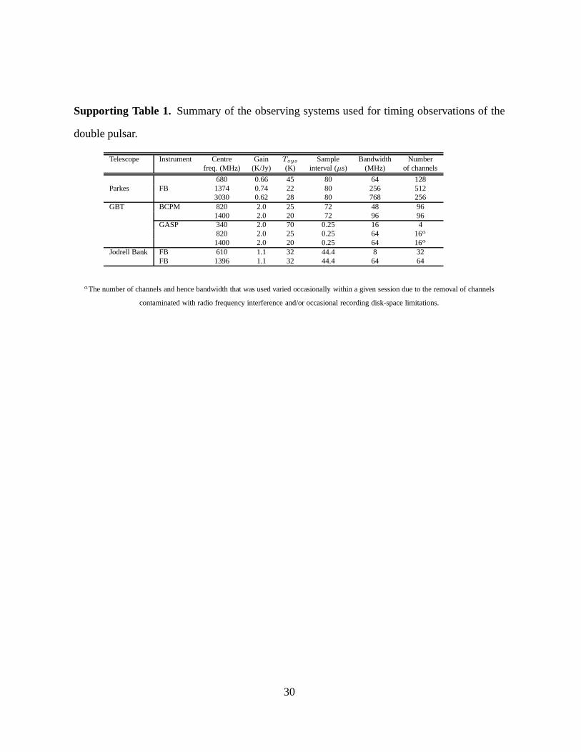
Supporting Table 1. Summary of the observing systems used for timing observations of the
double pulsar.
Telescope Instrument Centre Gain Tsys Sample Bandwidth Numberfreq. (MHz) (K/Jy) (K) interval (µs) (MHz) of channels
680 0.66 45 80 64 128Parkes FB 1374 0.74 22 80 256 512
3030 0.62 28 80 768 256GBT BCPM 820 2.0 25 72 48 96
1400 2.0 20 72 96 96GASP 340 2.0 70 0.25 16 4
820 2.0 25 0.25 64 16a
1400 2.0 20 0.25 64 16a
Jodrell Bank FB 610 1.1 32 44.4 8 32FB 1396 1.1 32 44.4 64 64
aThe number of channels and hence bandwidth that was used varied occasionally within a given session due to the removal of channels
contaminated with radio frequency interference and/or occasional recording disk-space limitations.
30
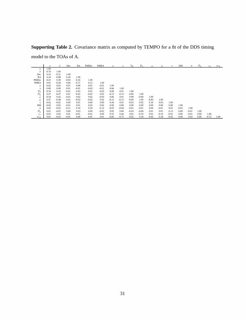
Supporting Table 2. Covariance matrix as computed by TEMPO for a fit of the DDS timing
model to the TOAs of A.
ν ν Dec RA PMDec PMRA x e T0 Pb ω ω γ DM π Pb zs m2
ν 1.00ν -0.76 1.00
Dec 0.16 -0.31 1.00RA 0.10 -0.08 0.18 1.00
PMDec -0.25 0.39 -0.83 -0.16 1.00PMRA 0.01 -0.28 0.04 -0.71 0.12 1.00
x -0.02 0.02 0.01 0.00 -0.01 -0.01 1.00e 0.00 0.00 0.01 -0.01 -0.02 -0.01 0.66 1.00
T0 -0.54 0.43 -0.01 0.02 0.02 -0.03 0.00 0.01 1.00Pb 0.47 -0.47 0.01 -0.02 -0.02 0.02 -0.15 -0.15 -0.85 1.00
ω -0.54 0.42 -0.01 0.02 0.02 -0.03 0.06 0.01 0.99 -0.84 1.00ω 0.47 -0.48 0.01 -0.02 -0.02 0.02 -0.15 -0.15 -0.85 1.00 -0.84 1.00γ -0.02 -0.02 0.00 0.01 0.00 0.00 0.44 0.01 -0.03 0.02 0.10 0.031.00
DM -0.02 0.02 -0.01 0.01 0.03 0.02 0.00 0.00 0.00 0.00 0.00 0.00 0.00 1.00π 0.05 -0.02 -0.21 0.16 0.20 -0.12 -0.03 -0.04 -0.01 -0.01 0.00-0.01 0.02 -0.02 1.00
Pb 0.01 -0.02 0.00 0.03 0.00 -0.02 0.05 0.00 -0.03 -0.06 0.01 0.01 0.13 0.00 -0.01 1.00zs -0.01 0.02 0.01 -0.01 -0.01 0.00 0.55 0.44 0.01 -0.10 0.01 -0.10 -0.01 0.00 -0.01 0.00 1.00
m2 0.01 -0.03 -0.01 0.00 0.01 0.01 -0.85 -0.75 -0.02 0.18 -0.02 0.18 -0.02 0.00 0.03 0.00 -0.72 1.00
31

Supporting Figure 1. Pulse profile templates used for TOA determinations for pulsar A.
Supporting Figure 2. Regions of orbital phase (hatched) used for timing of pulsarB and pulse
profile templates for these phases derived from and used for the 820 MHz GBT observations
in May 2005. Each of the template plots covers a range of60/360 = 0.17 in pulse phase.
Similar but different templates were used for other frequencies and epochs. While B was clearly
detectable in these three regions, it is actually brightestin the two cross-hatched regions, but
because the shape of the profile evolves quickly and dramatically in these regions, they were
excluded from the timing analysis.
Supporting Figure 3. Timing residuals obtained for pulsar A for the three telescopes and their
distribution. The upper panel shows the distribution of observations in frequency.
Supporting Figure 4. Timing residuals obtained for pulsar B for Parkes and the GBTand their
distribution. The upper panel shows the distribution of observations in frequency.
32
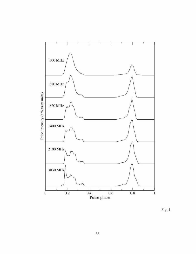
Fig. 1
33
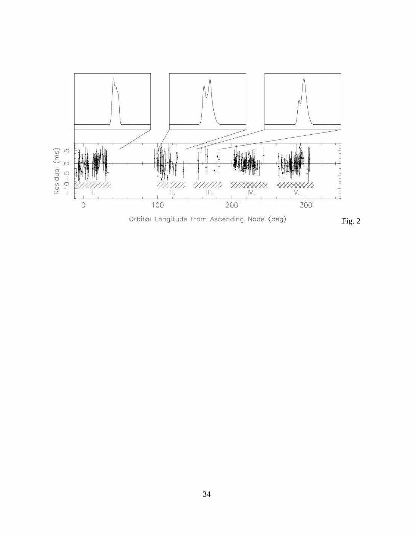
Fig. 2
34

Fig. 3
35

Fig. 4
36
Recommended