j
NASA-CR-199995 - '"
JOURNAL OF GEOPHYSICAL RESEARCH, VOL. 100, NO. D5, PAGES 9073-9090, MAY 20, 1995
Stratospheric aerosol and gas experiments I and II
comparisons with ozonesondes
Robert E. Veiga
Science Applications International Corporation, Hampton, Virginia
J
Derek M. Cunnold
Georgia Institute of Technology, Atlanta
William P. Chu and M. Patrick McCormick
NASA Langley Research Center, Hampton, Virginia
Abstract. Ozone profiles measured by the Stratospheric Aerosol and Gas Experiments(SAGE) I and II are compared with ozonesonde profiles at 24 stations over the periodextending from 1979 through 1991. Ozonesonde/satellite differences at 21 stations withSAGE II overpasses were computed down to 11.5 km in the midlatitudes, to 15.5 km
in the lower latitudes, and for nine stations with SAGE I overpasses down to 15.5 kin.The set of individual satellite and ozonesonde profile comparisons most closelycolocated in time and space shows mean absolute differences relative to the satellitemeasurement of 6 -- 2% for SAGE II and 8 +- 3% for SAGE I. The ensemble of
ozonesonde/satellite differences, when averaged over all altitudes, shows that forSAGE II, 70% were less than 5%, whereas for SAGE I, 50% were less than 5%. Thebest agreement occurred in the altitude region near the ozone density maximum wherealmost all the relative differences were less than 5%. Most of the statistically significantdifferences occurred below the ozone maximum down to the tropopause in the regionof steepest ozone gradients and typically ranged between 0 and -20%. Correlationsbetween ozone and aerosol extinction in the northern midlatitudes indicate that
aerosols had no discernible impact on the ozonesonde/satellite differences and on theSAGE II ozone retrieval for the levels of extinction encountered in the lower
stratosphere during 1984 to mid-1991.
Introduction
Over the last 3 decades, vertical profiles of ozone extend-ing from the ground into the lower stratosphere have beenroutinely measured by balloon-borne instruments (ozone-sondes) at a number of stations located predominantly in thenorthern hemisphere. With the advent of space-based plat-forms it became possible to measure ozone profiles withexpanded coverage over the Earth. The longest record ofsatellite-based high vertical resolution ozone profiles hasbeen generated by the Stratospheric Aerosol and Gas Ex-periments (SAGE) I and II, both developed at NASALangley Research Center [McCormick et al., 1979; Mauldinet al., 1985]. Both the ozonesonde and the satellite data have
been extensively used to quantify the processes governingatmospheric ozone variation. This paper presents the resultsof a statistical comparison designed to estimate any altitudedependent relative bias between the ozonesonde and thesatellite measurements•
SAGE I and SAGE II are conceptually identical multi-channel spectrophotometers which sense solar intensitythrough a slant path in the atmosphere as the instrumentorbits into (sunset) or out of (sunrise) the Earth's shadow.Ozone measurements are made in the Chappuis region of the
Copyright 1995 by the American Geophysical Union.
Paper number 94JD03251.0148-0227/95/94JD-03251 $05.00
spectrum at 600 nm with a vertical resolution of 1 kmthrough a slant path in the atmosphere approximately 220 kmin length at any given altitude. The quality of the measure-
ment in the lower stratosphere depends primarily on theextent to which interfering species such as aerosols or otherabsorbers can be accurately removed in the ozone retrieval[Chu and McCormick, 1979; Chu et al., 1989]. In addition tothe 600 nm channel, SAGE I utilized transmission measure-ments at 1000, 450, and 385 nm while SAGE II utilizeschannels at 1000, 940, 525,453,448, and 385 nm to charac-
terize other species. The ozone measurement's quality in thetroposphere is impacted by the presence of clouds andaerosols in the instrument field of view. A unique aspect ofthe solar occultation measurement is that long-term sensordrift is effectively removed via an exoatmospheric calibra-tion made during every profile measurement [Watson et al.,1988]. CunnoM et al. [1989] provided the following errorestimates for SAGE I and SAGE II in the altitude region of24-36 km: 7% systematic bias, 5% random error, and refer-ence altitude uncertainties of 0.25 km (SAGE I) and 0.2 km(SAGE II). An analysis of the error budget of the differencebetween SAGE I and SAGE II ozone retrievals over these
altitudes yields an expected systematic error of 6% at 20 kmand 2% between 25 and 30 km [Watson et al., 1988].
One characteristic of the occultation measurements is thatthe instrument makes at most one sunrise and one sunset
profile per orbit. The orbital inclinations of SAGE I and II
9073
https://ntrs.nasa.gov/search.jsp?R=19960016566 2018-07-16T08:33:52+00:00Z

9074 VEIGA ET AL.: SAGE 1 AND II COMPARISONS WITH OZONESONDES
yield patterns of observations whose latitudes vary slowly
with time. The latitudes ranging from 80°S to 80°N are
sampled in a period of about 1.5 months; however, only the
range from 50°S to 50°N are sampled every season of the
year. SAGE I was launched in February 1979 and operated
until November 1981. SAGE II was launched in October
1984 and continues to provide measurements. Studies using
the SAGE II ozone data set have included analyses of the
ozone quasi-biennial and semiannual oscillations (QBO and
SAO), Antarctic and Arctic springtime ozone variabilities,
and global ozone trends [McCormick and Larsen, 1988,
McCormick et al., 1989a,b; Zawodny and McCormick,1991].
Ozonesondes are launched on balloons at various stations
throughout the world at regular intervals. The types of
sondes in most common use are the electrochemical concen-
tration cell (ECC) [Komhyr, 1969; Komhyr and Harris,
1971], the Brewer-Mast (BM) bubbler [Brewer and Milford,
1960], and the carbon-iodine (CI) sonde [Komhyr, t965].
Each of these sondes employs the same method whereby
ozone is measured by pumping ambient air through an
electrolytic cell containing a buffered potassium iodide solu-
tion where ozone oxidizes the iodide into iodine. The result-
ant cell reaction current is directly proportional to the ozone
concentration in the cell. The major differences between
sonde types lie in the design of the cell and the electrolyte
concentrations. All ozonesondes are flown on a balloon with
a radiosonde for pressure and temperature data. After data
reduction the ozone is converted into units of partial pres-sure.
Above the burst altitude of the balloon the upper level
ozone amount must be taken into account if the integral of
the ozonesonde profile is to be used to estimate total ozone
above the station. During data reduction, the residual ozone
above the burst altitude is estimated by extrapolation of the
measured profile along contours of constant mixing ratio.
Furthermore, the ozonesonde output is not an absolute
measurement of the ozone profile, since ozone losses occur
within the instrument, and the instrument has a finite re-
sponse time [De Muer and Malcorps, 1984]. In order to
compensate for these deficiencies it has been general prac-
tice to multiply the measured ozone profile by the ratio of the
total ozone amount measured at the site by a Dobson
spectrophotometer to the total ozone amount derived from
integration of the ozonesonde profile. This ratio, called the
correction factor, is used by almost all stations as an altitude
independent scaling factor which makes the measured
ozonesonde profile consistent with the Dobson measure-
ment. However, in some cases the correction factor is not
available in the ozonesonde data set. A large deviation of the
correction factor from unity is usually indicative of measure-
ment errors in the ozonesonde profile. Tabulated mean
correction factors indicate that correction factor deviations
are, on average, less than 20% and depend on the station
[Logan, 1985]. Some stations exhibit temporal trends in the
correction factors indicating long-term changes in sonde
flight calibration [Tiao et al., 1986].
Systematic errors in the ozonesonde measurement can
arise from altitude-dependent pump efficiency [Komhyr and
Harris, 1965; Torres, 1981; Harder, 1987], background cur-
rent correction [Komhyr and Harris, 1971; Thornton and
Niazy, 1982, 1983], frequency response of the sensor and
air-sampling system [De Muer and Malcorps, 1984], electro-
lyte concentration, extrapolated upper level column amount,
and altitude determination [Schmidlin, 1988]. Tests con-
ducted on ECCs in a controlled laboratory environment
indicate an accuracy of 3--5% positive error from 300 to 50
hPa and 10% from 50 to 15 hPa with precision estimates of
5-6% from 200 to 10 hPa [Barnes et al., 1985]. These results
are in overall agreement with the Balloon Ozone Intercom-
parison Campaign (BOIC) which was designed to assess the
accuracy and precision of atmospheric ozone measuring
instruments [Hilsenrath et al., 1986]. ECC ozonesonde error
assessments performed by Komhyr et al. [1994] indicate 6%
accuracy and 3% precision from 100 to 10 hPa.
Other SAGE I/II Comparisonswith Ozonesondes
Several comparisons between SAGE I/SAGE II and
ozonesondes have been performed largely as satellite instru-
ment validation studies not specifically addressing the pos-
sibility of altitude dependent systematic relative biases be-
tween the two ozone measuring methods [McCormick and
Reiter, 1982; McCormick et al., 1984; Attmannspacher et
al., 1989; Cunnold et al., 1989; Margitan et al., 1989; WMO,
1990; Barnes et al., 1991 ; De Muer et al., 1990; McDermid et
al., 1990]. De Muer et al. [1990], for example, analyzed a
sample of 24 colocated profile pairs (0.3 day and 600 km) at
Uccle. The SAGE II/Brewer-Mast differences over the
altitude range from 10-26 km indicated SAGE II was lower
in column amount by 4% than the sondes. On the other hand,
SAGE II was higher than the sondes by 3.3% between 26 and
31 km. In Barnes et al. [1991], samples of 14 SAGE II
profiles were compared with seven ECC profiles during a
correlative mission at Natal, Brazil, in March and April
1985, and a difference profile was estimated over the altitude
range from 17.5 to 24.5 km. From 20.5 to 24.5 km, SAGE II
was within 0.5% of the ECC measurements. Below 20.5 km
the 95% confidence intervals were large due to atmospheric
variability and included 0%. Cunnold et al. [1989] computed
the relative difference between a sample of five colocated
measurements between SAGE II and ECCs over the altitude
range from 15.5 to 25.5 km, and their results were consistent
with those presented herein. Cunnold and Veiga [1991]
presented a comparison between SAGE I/II and ozone-
sondes which showed larger ozonesonde/SAGE I differences
than ozonesonde/SAGE II differences and general altitude
dependent differences maximizing between 16 and 18 kin.
The work presented herein is an extension of their method
which utilizes an expanded set of ozonesonde and SAGE I/IIdata.
All of the previous published comparisons described
above were performed using a version of the SAGE II data
set earlier than that used here. The version used here
(version 5.9) has improvements in the aerosol correction to
the ozone below 15 km, and a long-term time-varying mirror
reflectivity correction which affects ozone concentration
above 50 km.
Data Description
The fundamental SAGE I/II measurement of ozone is
number density as a function of geometric altitude at 1 km
increments. Transformation to a pressure altitude coordinate
involves using National Meteorological Center (NMC) data

VEIGAETAL.:SAGEI ANDII COMPARISONSWITHOZONESONDES 9075
interpolatedto theSAGEI/II location,aprocedurewhichaddsanunnecessarylevelofuncertainty.Thusthecompar-isonswereperformedon a geometricaltitudescalebytransformingtheozonesondedatafrompressurealtitudetogeometricaltitude.Therationalefor usingthisaltitudecoordinateisthattheozonesondepressureandtemperaturemeasurementsrepresentamoreaccuraterepresentationoflocalconditionsthandothepressureandtemperaturedatainterpolatedfromtheNMC-griddedanalysis.Theozone-sondeprofilesweremappedto a geometricaltitudescaleusingthehypsometricequationwithgravitationalaccelera-tionvariablewith latitudeandaltitude[List, 1951].Nohumiditydatawereavailablefor theozonesondeprofiles,andthusthemeanmolecularweightwasassumedconstant.Ozonesondemeasurementswereconvertedfrompartialpressureto numberdensity.Thereareerrorsinherentinusingthehypsometricequationtoobtaingeometricaltitudeandinconvertingpartialpressureto numberdensityfromradiosondepressureandtemperaturemeasurements.Par-
sons et al. [1984] compared highly accurate radar altitudes
with altitudes constructed through the hypsometric equation
using U.S. radiosonde measurements, and they derived
altitude errors (rms) of up to 600 m at 30 km and 250 m at 25
km. Schmidlin [1988] intercompared radar altitudes with
hypsometric altitudes derived from closely matched multiple
soundings of several well-calibrated radiosonde types in
worldwide use. Their results were inconclusive regarding the
sign of any potential altitude difference. Near 18 km the
radiosonde/radar altitude difference and standard deviation
were both less than approximately 100 m, indicating rela-
tively good agreement among the various sonde types.
However, near 24 km both the altitude difference and
standard deviation ranged from 100 to 500 m among the
sonde types.
Most of the profiles in the ozonesonde database are
corrected for the total ozone amount as part of the standard
data reduction process at the ozonesonde station. Profiles
from stations for which the Dobson correction is not applied
as part of the standard data processing were corrected for
this study. Furthermore, each ozonesonde profile was mul-
tiplied by 0.9743 to account for the currently accepted ozone
cross sections used in the Dobson measurement [Bass and
Paur, 1985; Komhyr, 1980]. Profiles were rejected from the
comparison whenever the correction factors were not in the
range 0.80-1.2. Profiles which had no corresponding Dobson
measurement available were used with no total ozone cor-
rections applied; however, the number of such profiles was
less than 6% of the total sample size of the ozonesonde data
set.
The ozonesonde/satellite sampling was set so that the
satellite-altitude coordinate ranged from cloud top to ap-
proximately 32 km, and the spatial location of the profiles
was taken at the latitude and longitude of the SAGE I/II 20
km tangent point. SAGE I/II profiles were not compared
with ozonesondes if local meteorological data was unavail-
able below 25 km (used for the Rayleigh extinction correc-
tion to the satellite ozone profile). The number of ozone-
sonde/satellite profile pairs (a pair is defined below) used in
computing a difference profile was based on a spatial-
temporal window (STW) which was large enough to make
the length of the 95% confidence interval on the difference
smaller than 20% at some point in the altitude region near the
peak of the ozone number density (21-26 km). Using this
criterion, the STWs for each station ranged from a maximum
of 2 days and 1000 km to 18 hours and 600 km. If more than
one SAGE I/II profile was within the STW, then all the
satellite profiles in the window were compared with the
single colocated sonde profile. Henceforth we shall refer to
the set of ozonesonde/SAGE colocated profiles as the
"paired data."
Table 1 lists the 24 ozonesonde stations for which suffi-
ciently large sample sizes of ozonesonde/SAGE colocations
occurred during the period of 1979-1991. Most stations used
the ECC. The Canadian stations (station numbers 21, 24, 76,
and 77) changed from using BM sondes to ECC sondes in
1979-1980, whereas the Japanese stations (7, 12, 14, 101, and
190) used the CI sonde. Figure 1 shows the distribution of
the ozonesonde station locations (triangles) superposed with
the sampling locations (squares) for the sunset meridional
sweep of SAGE II during March (SAGE I sampling is
similar).The SAGE I and SAGE II data set were provided by the
NASA Langley Research Center, Hampton, Virginia, and
were also available through the National Space Science Data
Center, Greenbelt, Maryland. The ozonesonde data sets
were provided by the World Ozone Data Center (WODC),
Downsview, Ontario; the National Oceanic and Atmo-
spheric Administration (NOAA), Boulder, Colorado; and
the National Institute of Water and Atmospheric Research,
Central Otago, New Zealand.
Difference Profiles
By utilizing the relatively large number of sampling oppor-
tunities available in the paired data, it was possible to
estimate the relative systematic difference between the in
situ electrochemical method and the satellite occultation
method. The underlying assumption was that the effect of
random variation would cancel, as the sample became large.
However, the spatial and temporal separation constraints
tend to keep the sample sizes from growing unlimitedly since
increasing each pair's spatial separation also increases the
probability of geophysically induced differences.
Vertical profiles of the percentage difference between the
ozonesonde measurement and the satellite measurement
referenced to the satellite measurement over the altitude
range of 15.5-32.5 km (SAGE I) and 10.5-32.5 km (SAGE II)
in 1 km increments were computed. The SAGE measure-
ment was chosen as the reference since it represents the
output of a unique self-calibrating instrument with constant
characteristics through time, whereas the ozonesonde pro-
files come from a variety of stations with interunit differ-
ences.The measure of difference chosen to estimate the ozone-
sonde/SAGE difference was the median percentage differ-
ence defined as
A = 100 • median (_-_),
where Y represents the vector of ozonesonde measurements
and X the corresponding vector of SAGE I/for measure-
ments in the colocated sample. Ninety-five percent confi-
dence intervals on A were computed using the bootstrap
technique [Efron, 1982]. As a consistency check, the collec-
tion of sample fractions, (¥ - X)/X, were also modeled with

9076 VEIGA ET AL.: SAGE I AND II COMPARISONS WITH OZONESONDES
Table 1. World Ozone Data Center Ozonesonde Stations
Latitude, Longitude, Elevation,Station deg deg m SAGE I Period SAGE II Period Sonde
12, Sapporo14, Tateno21, Edmonton24, Resolute67, Boulder
76, Goose Bay77, Churchill
99, Hohenpeissenberg101 Syowa107 Wallops Island109 Hilo
132 Sophia156 Payerne174 Lindenberg190 Naha191 Samoa
197 Biscarrosse210 Palestine
215 Garmisch233 Marambio254 Laverton256 Lauder
262 Sodankyla
265, Irene 25S 28E 1524 ECC
43N 141E 19 Oct. 1986 to June 1991 CI
36N 140E 31 Nov. 1984 to April 1991 CI54N I I4W 766 Feb. 1979 to Nov. 1981 Aug. 1985 to June 1991 ECC75N 95W 64 May 1979 to Sept. 1981 Aug. 1985 to April 1991 ECC40N 105W 1743 Jan. 1985 to Feb. 1990 ECC
53N 60W 44 March 1979 to Sept. 1981 Nov. 1984 to June 1991 ECC59N 94W 35 March 1979 to Sept. 1981 Oct. 1984 to June 1981 ECC48N liE 975 Feb. 1979 to Nov. 1981 Oct. 1984 to June 1991 BM69S 40E 21 Dec. 1984 to Oct. 1990 CI
38N 76W 13 March 1979 to Nov. 1981 Nov. 1984 to May 1991 ECC20N 155W 11 Dec. 1984 to Nov. 1990 ECC
43N 23E 58 Nov. 1984 to April 1991 Unknown47N 7E 491 Feb. 1979 to Sept. 1981 Unknown52N 14E 98 May 1979 to Nov. 1981 Oct. 1984 to April 1991 ECC
26N 128E 27 Sept. 1989 to July 1991 CI14S 170W 82 July 1986 to March 1988 ECC
44N IW 18 May 1979 to Nov. 1981 BM
32N 96W 210 May 1985 to May 1985 ECC48N llE 740 Feb. 1979 to Nov. 1981 BM
64S 57W 198 Nov. 1988 to April 1991 ECC38S 144E 21 July 1986 to Oct. 1990 BM45S 170E 370 Sept. 1986 to Dec. 1990 ECC68N 27E 179 March 1989 to April ECC
1991
July 1990 to May 1991
Ozonesonde stations for which SAGE I/II overpassed within a window of 24 hours and 1000 km. CI is Carbon-Iodine; ECC iselectrochemical concentration cell; BM is Brewer-Mast.
90
70
50
30
[
10
SAGE II Locations 26-Feb-1988 to 2-Apr-1988 Sunset
o
D
O []
i i
,iO 0 :
0
o []
Cl [] O O
[] q ......... 0 .........
[] o D 0[] 0 [] []
D [] []D 0 []
[]
0
0 [] []
0 o
::o []
o []
[] £
[]
D 0
o :0o o
io.........o...._ o: [] O i O
0 [] : [][] [] O0 [] []
[]Oi[]:D
o o
[] []
[] []
0 : 0
m rn O
[]
O 0 i O[] 0 [D0 0 [][]
0
D[]
[]
[]
-70
-90
-180 -135 -90 -45 0 45 90 135 180
Figure 1. Ozonesonde locations (triangles) and SAGE II sampling locations for February-April 1988(squares). The circle around the Wallops Island station is 1000 km in radius.
VEIGA ET AL.: SAGE I AND II COMPARISONS WITH OZONESONDES 9077
(a) 35
30
25
I0
5
0
o,1
(c) 35
30
25
10
-14.3 189.4 82 Samoa (191)i
Year 1988
WODC day II ,_.SAGE day I0SAGE profile 4 sunsetDT 38 hoursDS 948 kmCF 0.00WODC
SAGE_
trop
1.0
03 ( xi0 n cm "s )
-25.3 28.2 1524 Irene (265)
I0.0
(b) 35
3O
25
10
5
0
o.1
iYear 1991
WODC day 16SAGE day 18SAGE profile 3 sunriseDT 43 hoursDS 447 kmCF 1.05WODC _------_
SAGE _ trop
I
(d) 35
30
25
15
10
5 5
0 00.1 1.0 10.0 0.1 1.0
0 3 ( xl0 n cm "3) 0 3 ( xl0 _ cm _ )
19.7 204.9 11 Hilo (109)Year 1986 ....... ' ......
WODC day 45SAGE day 45SAGE profile 3 sunsetDT 15 hoursDS 415 kmCF 1.13WODCSAGE m******_ trep
1.0 10.0
03 ( xlO n cm "_)
26.2 127.7 27 Naha (190)
Year 1991 ....... ' .....
WODC day 184SAGE day 184 -'h_SAGE profile 7 sunset "_DT 4 hours DDS 644 km apCF 0.94WODC_----,
SAGE_ tr_
10.0
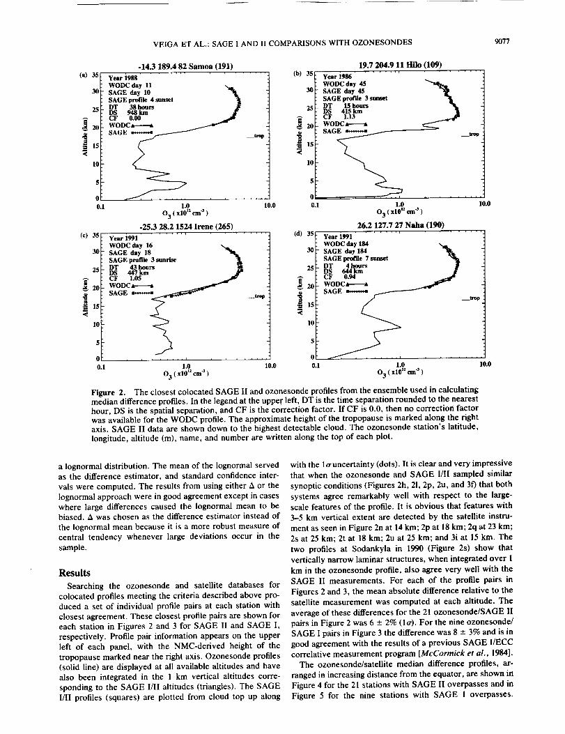
Figure 2. The closest colocated SAGE II and ozonesonde profiles from the ensemble used in calculatingmedian difference profiles. In the legend at the upper left, DT is the time separation rounded to the nearesthour, DS is the spatial separation, and CF is the correction factor. If CF is 0.0, then no correction factorwas available for the WODC profile. The approximate height of the tropopause is marked along the rightaxis. SAGE II data are shown down to the highest detectable cloud. The ozonesonde station's latitude,longitude, altitude (m), name, and number are written along the top of each plot.
a lognormal distribution. The mean of the lognormal servedas the difference estimator, and standard confidence inter-
vals were computed. The results from using either A or thelognormal approach were in good agreement except in caseswhere large differences caused the Iognormal mean to bebiased. A was chosen as the difference estimator instead of
the lognormal mean because it is a more robust measure ofcentral tendency whenever large deviations occur in the
sample.
Results
Searching the ozonesonde and satellite databases forcolocated profiles meeting the criteria described above pro-duced a set of individual profile pairs at each station withclosest agreement. These closest profile pairs are shown foreach station in Figures 2 and 3 for SAGE II and SAGE I,respectively. Profile pair information appears on the upperleft of each panel, with the NMC-derived height of thetropopause marked near the right axis. Ozonesonde profiles(solid line) are displayed at all available altitudes and havealso been integrated in the 1 km vertical altitudes corre-sponding to the SAGE I/II altitudes (triangles). The SAGEI/II profiles (squares) are plotted from cloud top up along
with the lo-uncertainty (dots). It is clear and very impressive
that when the ozonesonde and SAGE I/II sampled similar
synoptic conditions (Figures 2h, 21, 2p, 2u, and 3f) that both
systems agree remarkably well with respect to the large-scale features of the profile. It is obvious that features with3-5 km vertical extent are detected by the satellite instru-
ment as seen in Figure 2n at 14 km; 2p at 18 kin; 2q at 23 kin;2s at 25 km; 2t at 18 kin; 2u at 25 km; and 3i at 15 km. The
two profiles at Sodankyla in 1990 (Figure 2s) show that
vertically narrow laminar structures, when integrated over 1km in the ozonesonde profile, also agree very well with theSAGE II measurements. For each of the profile pairs in
Figures 2 and 3, the mean absolute difference relative to thesatellite measurement was computed at each altitude. The
average of these differences for the 21 ozonesonde/SAGE IIpairs in Figure 2 was 6 -+ 2% (l_r). For the nine ozonesonde/SAGE I pairs in Figure 3 the difference was 8 -+ 3% and is ingood agreement with the results of a previous SAGE I/ECCcorrelative measurement program [McCormick et al., 1984].
The ozonesonde/satellite median difference profiles, ar-
ranged in increasing distance from the equator, are shown inFigure 4 for the 21 stations with SAGE II overpasses and in
Figure 5 for the nine stations with SAGE I overpasses.

(e) 35
30
25
30
15 _i
10
5
0
0.1
(s) 3s
30
25
i
10
5
Oi
0.1
31.8 264.3 121 Palestine (210)...... i
Year 1985WODC day 136 _.SAGE day 136SAGE prollle 8 sunrise
7 hours
WOi_----_SAGE
trep
1.0 10.0
0 3 ( xl0 u cut _ )
37.8 284.5 13 Wallops Island (i07)
Year 1990WODC day 277SAGE day 278 -_SAGE profile 7 sunrise "_DT 19 hoursDS 784 kmCF 1.00 _ffwoven------,
SAG_
...... trop
1.0 10.0
0 3 ( xlO I=cm "_)
(h) 35
30
25
10
5
0
0.1
(i) 3$
3O
25
30
10
5
00.1
(k) 35
30
25
10
40.0 254.8 1743 Boulder (67)...... i .......
Year 1985
WODC day 211SAGE day 211SAGE profile 8 sunriseDT 4 hoursDS 598 kmCF 0.99WODC _-----_SAGE
trop
1.0
0 3 ( xl0 TMcm "3)
43.0 141.3 19 Sapporo (12) .......
Year i987 ....... '
WODC day 259
SAGE day 259 "_SAGE profile 6 sunsetDT 3 heursDS 337km 1,CF 1.14 ._rwoDc.------_
SAGE_
...o. ..... -."
5
00.1 1.0
0 3 ( xl0 u cm _ )
mtrop
(j) 35
3_
25
• _ 15
10
5
0
10.0 0.1
,0.0
Figure 2.
(I) 35
30
25
10
5
0
0.1
42.8 23.4 588 Sofia (132)....... i
Year 1986
WODC day 141SAGE day 141
SAGE profile 2 sunriseDT 9 hoursDS 687kmCF 1.12WODCSAGE _..***m
trop
1.0 10.0
0 3 ( xl0 u cm "_)
-45. 0 169.7 370 Lander (256! ......Year 1987
WODC day 187SAGE day 187SAGE profile 13 sunriseDT 2 hoursDS 265kmCF 0.99WODCSAGE l******_
. _ trop
t.0 10.0
0 3 ( xlO n cm "3)
36.0 140.1 31 Tateno (14) ........
Year i990 ........
WODC day 206
SAGE day 305SAGE profile 13 sunriseDT 10 hoursDS 514 kmCF 0,99WODCSAGE _****_
trep
(continued)

(m)35
30
25
15
10
5
0
0.1
(o) 35
30
25
]1,10
$
0
0.1
47.8 11.0 975 Hohenpeissenberg (99)
Year i986 ....... ' ........
WODC day 34SAGE day 34SAGE profile 11 sunsetDT 9 hoursDS 383kmCF 1.03WODCt-----tSAGE
I
1.0 10.o
0 3 ( xlO TM cm "s)
53.3 299.6 44 Goose Bay (76)
Year i_0 ...... '
WODC day 318 t_SAGE day 318SAGE profile 11 sunsetDT 10 hoursDS _O lensCF 1.00WODC_------_SAGE m*****_
._ trep
1.0 10.0
0 3 ( xl0 n cm "3)
(n) 35
30
25
10
5
o
0.!
(p) 3S
3O
25
_ 15
10
5
0
0.1
52.2 14.1 98 Lindenberg (174)...... I
Year 1990WODC day 108SAGE day 107SAGE profile 12 suaset
,%.
DT 17 hours "_DS 744 kmCF 1.19WODC t-------tSAGE m***.*_
trep
1.0
03 ( xl0 u cm "3)
53.6 245.9 766 Edmonton (21)...... n ........
Year 1998WODC day 141SAGE day 141SAGE profile 8 sunrise
I hours
WOIN2 _SAGE _,**.*m
10.0
1.0
0 3 ( xl0 n cm "3)
10.0
(q) 35
3O
25
10
5
00.1
(s) 35
3O
25
],,10
5
0
0.1
58.8 265.9 35 Churchill (77)
Year i9S6 ........
WODC day 218SAGE day 218SAGE profile 7 sunriseDT 0 hearsDS 564kmCF 0.98WODC t-------tSAGE m**.**m
trep
1.0
03 ( xl0 u ¢m -_ )
67.5 26.6 179 Sodankyla (262)
Year i_90 ........
WODC day 73SAGE day 73SAGE profile 4 sunriseDT 7 hoursDS 662 kmCF 1.14WODCSAGE
10.0
1.0
0 3 ( xl0 u cm "3)
10.0
(r) 35
3O
25
15
l0
5
0
0.!
(t) 35
M
25
10
5
0
OA
-64.2 303.3 198 Marambio (233)
Year i988 ........ " ....... tWODC day 329 ]SAGE day 325 -_
SAGE profile $ sunrise "_DT 27 hours _ -]DS 594 km =_CF 0.0o "_t twoDc,---_ ]L
S-- l1.0 10.0
0 3 ( xl0 u cm "3)
-69.0 39.6 21 Syowa (101)
Year 1988
WODC day 279 tl_SAGE day 278SAGE profile 11 sunsetDT 17 hoursDS 405 kmCF 0_9WODC Jr----_SAGE
L0
0 3 ( xlO u cm "j)
trop
10.0
Figure 2. (continued)

9080 VEIGA ET AL.: SAGE I AND II COMPARISONS WITH OZONESONDES
(u) 35
30
25
20
,¢
lO mtrop
74.7 265.0 64 Resolute (24),iYear 1988
WODC day 223 __SAGE day 223SAGE profile 6 sunriseDT 2 hoursDS 377 kmCF 0.94WODCSAGE
LO
0 3 ( xl012cm "3)
00.1 10.0
Figure 2. (continued)
Because of the limited data availability, not all years are fully
represented, and the reader is referred to Table 1 for the
dates. Each panel of difference profiles lists the total number
of samples available at each altitude along the right axis.
Ninety-five percent confidence intervals are represented by
the dotted band. Each profile is shown down to only those
altitudes where the length of the 95% confidence interval was
less than 20%. Although difference estimates were computed
below the lowest altitudes shown in Figures 4 and 5, the
combination of small sample sizes along with large variabil-
ity of the median difference precluded the estimation of the
ozonesonde/satellite bias with a high degree of confidence.
For Samoa (Figure 4a), almost all differences are not
significant for the altitudes 21.5-31.5 km. The Hilo data
(Figure 4b) indicate SAGE II ozone is larger by 8% above 17
km. There is no apparent altitude trend in the difference
profile shape, a feature indicative of good altitude registra-
tion in the satellite measurement. A characteristic tendency
for many comparisons (Figures 4c-4h, 4m, and 4q) is good
agreement near the peak of the ozone profile and a subse-
quent divergence to significant negative differences below
the peak. This effect is most pronounced equatorward of 40 °
and may be related to the steep gradient between the ozone
peak and the tropopause at these latitudes. Figure 4e shows
the comparison at Palestine which was organized as part of
a SAGE II correlative measurement program in 1985. Al-
though the sample size is small, there are no significant
differences between 20.5 and 30.5 km. Poleward of 45 °, all
but one comparison had data extending below 14 km (Fig-
ures 41-4u) which showed no significant differences at the
lowest altitudes. The exception is Syowa in Antarctica
where the difference is between - 10 and -5% below 23 km.
This altitude range at Syowa coincides with the ozone
depletion region during Antarctic spring when SAGE II
samples these polar latitudes densely. Ozone gradients as-
sociated with the vortex may have caused the differences in
the Syowa comparison. The greatest number of colocations
per sampling window size occurred at Hohenpeissenberg
(Figure 4m). For this station the difference profile exhibits
negative values up to -10% above 32 km and also below the
ozone density maximum. The negative differences at the
upper altitudes may be due to reduced air pump efficiency of
the Brewer-Mast sonde. The largest ozonesonde/satellite
deviations occur in the Lindenberg comparison (Figure 4n)
above 25 km where the differences reach -20% at 31.5 km.
An assessment of the relative ozonesonde/SAGE II differ-
ence using the difference profiles of Figure 4a-4u was
performed by enumerating the differences less than 5% in
magnitude at each altitude. These "5%" differences are
shown in Figure 4v as the shaded region of a rectangle whose
length is the total number of differences for a given altitude.
Between 21 and 30 km at least 15 stations had absolute
differences less than 5%, with the best count at 24.5 km
where all but Hilo agreed to better than 5%. Between 14.5
and 20.5 km and at 31.5 km about half the ozonesondes
agreed with SAGE II to within 5%. From the combined
stations, differences were estimated at 343 altitudes, and at
240 of those altitudes the median differences were less than 5%.
The comparisons with SAGE I are shown for nine stations
in Figures 5a-5i. 95% confidence intervals of length 20%
were not available below 15 km. Except for the northern-
most station the profiles show increasingly negative values
as the altitude decreases below the ozone maximum, culmi-
nating in differences between -20 and -10% near 15.5 km.
Except for Payerne (Figure 5c), which shows an overall
difference of -10%, all the stations agree well near the
maximum of the ozone density. At all but one station the
differences at the upper altitudes show increasingly negative
values with increasing altitude, the extreme case being
Resolute (Figure 5i) with -16% at 31.5 km but with few
coincident comparisons.
The combined differences for SAGE I are shown in Figure
5j, and are consistent with the SAGE II tabulated differences
(Figure 4v) in the altitude range near the ozone maximum.
However, below 20 km less than half the stations showed
agreement within 5% with SAGE I. No confidence intervals
of 20% in length were available below 15 km. From the
combined stations, differences were estimated at 138 alti-
tudes, and at 71 of those altitudes the median differences
were less than 5%.
The tendency for some of the difference profiles (Figures
4b, 4c, 4d, 4t, 4g, 4h, 4k, 4m, 4p, 4q and Figures 5a-5h) to
exhibit trends toward negative values as the altitude de-
creases below the ozone maximum may, in part, be due to
the ozonesonde measurement. In the region of rapid ozone
increases above the tropopause, the measured ozonesonde
profile is the convolution of the true ozone profile with the
sonde instrument temporal response function. De Muer et
al. [1990] reported better agreement between 24 colocated
ozonesonde and SAGE II profiles at Uccle when the instru-
ment response function was deconvolved from the measured
sonde profile. Comparisons of the measured ozonesonde
profiles at Uccle with their corresponding deconvolved
profiles indicate a mean difference (measured-deconvolved)
of -3 --- 1% at 15 km, whereas at 30 km the mean difference
is 6 -+ !% (D. De Muer, personal communication, 1990). This
positive difference at 30 km contrasts with the ozonesonde/
SAGE II difference profiles shown in Figure 4 where nega-
tive differences appear at 30 km, and may be indicative that
declining pump efficiency has a stronger effect than sonde
response on the ozone measurement. Additional evidence
supporting the sonde temporal response's effect on the
measured profile is found in the BOIC study where differ-
ences of approximately 10% between UV photometers and
ECCs were recorded in the vicinity of 80 hPa with the UV
photometers measuring higher ozone than the sondes. These

VEIGA ET AL.: SAGE 1 AND II COMPARISONS WITH OZONESONDES 9081
(a) 35
30
25
so
lO
o
0.1
(c) 35
30
25
_20
37.8 284.5 13 Wallops Island (107)i
Year 1981WODC day 195 _m,_.SAGE day 196SAGE prof'de 1 sunsetDT 10 hoursDS 540 kmCF 1.01WODCSAGE m..***_
trop ._
1.0
0 3 ( XI012 cm 3 )
46.8 7.0 491 Payerne (156)
Year 1980
WODC day 213SAGE day 213SAGE profile 12 sunsetDT 5 hoursDS 256 kmCF 1.05WODCSAGE
10.0
15
10
5
00.1
Figure 3.
_ trop
\
1.0 10.0
0 3 ( xl0 n em "3)
(b) 35
30
25
_20
._ 15
1o
o
0.1
(d) 35
30
25
20
•= 15
10
44.4 358.8 18 Biscarrosse (197)i
Year 1980WODC day 77SAGE day 77SAGE profile 12 sunsetDT 4 hoursDS 299 kmCF 1.17WODC t-------_SAGE
trop
1.0
0 3 ( xl0 n cm-_ )
47.5 11.1 740 Garmisch (215)
10.0
iYear 1980
WODC day 347SAGE day 347 _.SAGE profile 9 sunsetDT 7 hoursDS 562 kmCF 1.19WODC _-----tSAGE
__t_p
o
0.1 1.0 10.0
0 3 ( xl0 tz cm "3)
The closest colocated SAGE I and ozonesonde profiles from the ensemble used in calculatingmedian difference profiles. In the legend at the upper left, DT is the time separation rounded to the nearesthour, DS is the spatial separation, and CF is the correction factor. If CF is 0.0, then no correction factorwas available for the WODC profile. The approximate height of the tropopause is marked along the rightaxis. SAGE I data are shown down to the highest detectable cloud. The ozonesonde station's latitude,longitude, altitude (m), name, and number are written along the top of each plot.
differences were attributed to the ECCs lagging the photom-
eters in the altitude region of a high ozone gradient
[Hilsenrath et al., 1986]. The difference profiles in Figures 4
and 5 are broadly consistent with those observed in BOIC.
Implications on the SAGE II/SAGE I Difference
The satellite comparisons with the ozonesondes at Wal-lops Island (Figures 4g and 5a), Hohenpeissenberg (Figures4m and 5e), Goose Bay (Figures 4o and 5f), Edmonton
(Figures 4p and 5g), and Churchill (Figures 4q and 5h)
provide an opportunity to address the validity of the lower
stratospheric trends computed using the SAGE I and SAGE
II data over the period of 1979 through 1991 where trends
were computed down to 17.5 km [McCormick et al., 1992].
Implicit here is the assumption that the ozonesonde instru-
ment quality, calibration, and analysis did not change
throughout the time period. Comparing the difference pro-
files at 17.5 km for each of the above stations between the
SAGE I and SAGE II time periods reveals that the 95%
confidence intervals overlap, and thus it cannot be inferred
that the difference between SAGE I and SAGE II ozone at
this altitude was nonzero. However, sampling the Hohen-
peissenberg data using a larger sampling window reduces the
size of the ozonesonde/SAGE I and II difference profile
confidence intervals, and yet the shape and location of the
difference profiles are essentially the same as in Figures 4m
and 5e. At 17.5 km the ozonesonde/SAGE I difference is
-15% while the ozonesonde/SAGE II difference is -9%.
This yields a SAGE I/II difference of 6%, and thus within the
estimated SAGE I/II uncertainty reported by Watson et al.
[1988] for the 20 km altitude. Thus we cannot conclude,
based on the Hohenpeissenberg data alone, that the SAGE
I/II difference at 17.5 km is statistically significant.
Aerosol Correlation and Temporal Stability
The relatively large paired data sample (1 day and 1000km) available at Hohenpeissenberg was used to assess thepotential influence of a wide dynamic range in aerosolextinction on the ozonesonde/sateUite difference. Figure 6shows the 1020 nm SAGE II aerosol extinction coefficient at
18.5 km in a 10° latitude band centered over 48°N, thelatitude of Hohenpeissenberg. Near 18.5 km the extinctionprofile takes on its stratospheric maximum at these latitudes,
and thus the time series in Figure 6 approximates, up to a
scaling constant, the time history of stratospheric optical
depth for this latitude band. It can be seen that the extinction

9082 VEIGAETAL.:SAGE I AND I1 COMPARISONS WITH OZONESONDES
(e) 35
3O
25
J
10
5
0
0.1
(g) 35
30
25
15
I0
5
0
0.1
47.8 11.0 975 Hohenpeissenberg (99)i
Year 1981
WODC day 264SAGE day 263SAGE prellle 9 sunsetDT 15 hoursDS 164 kmCF 1.11WODC*------_SAGE a**-.*.-m
trop
1.0
0 3 ( xl0 TM cm -3)
53.6 245.9 766 Edmonton (21)
10.0
iYear 1980
WODC day 282SAGE day 283SAGE profile I sunsetDT 14 hours!_ 429 lanCF 1.15WODCSAGE
trap
I
1.0
0 3 ( xl012 cm "3)
10.0
(13 35
30
25
15
10
5
0
0.1
(h) 35
30
25
10
5
0
0.!
53.3 299.6 44 Goose Bay (76)i
Year 1980
WODC day 73SAGE day 73SAGE profile 14 sunsetDT 0 hoursDS 595 kmCT 1.09WODCSAGE
_.._----__,_
1.0
0 3 ( xl012 ¢nf 3 )
58.8 265.9 35 Churchill (77)
10.0
iYear 1981
WODC day 259SAGE day 259 :_SAGE profile I sunsetDT 10 hoursDS 547 kmCF 1.13WODC *------_SAGE s******_
1.0
0 3 ( xl0 n cm "3)
10.0
Figure 3. (continued)
time history began a decline from the large values in 1984-
1985, which were predominantly the volcanic aerosol rem-
nants of the 1982 eruption of El Chich6n (18°N), to highly
variable values in early 1986 driven by the Nevado Del Ruiz
(5°N) eruption in late 1985, and subsequently to the low
values in early 1991. Each year was punctuated by large
winter variances induced by the intrusion of polar air masses
and small summer variances. Significant stepwise decreases
in the mean aerosol amount occurred during the springs of
1985, 1988, and 1991 and may be related to QBO modulated
advection to the high latitudes. After mid-1991, the Mount
Pinatubo (15°N) eruption caused large increases in extinction
[McCormick and Veiga, 1992].
To assess the potential impact of less extreme aerosol
loading than that produced by Mount Pinatubo, the ozone-
sonde/SAGE II differences at Hohenpeissenberg were ana-
lyzed in order to determine whether a time dependent
correlation existed between the ozone differences and aero-
sol extinction. The presence of larger correlations during
periods of time when the aerosol extinction was higher than
during periods when the extinction was lower would be
indicative that the SAGE II ozone retrieval contained an
aerosol residual. Several time periods of varying length were
chosen so that each period could be clearly classified as
having high, medium, or low aerosol amount (Figure 6:
1984-1985, 1986--1987, and 1989-1990, respectively). Corre-
lation coefficients of the ozonesonde/SAGE II difference
versus the SAGE II 1020 nm extinction were computed over
the altitude range from 10.5 to 32.5 km, and the resulting set
of three correlation profiles possessed a high degree of
similarity irrespective of the period each represented. The
temporal constancy of the correlation profile indicates that
for the aerosol levels encountered between late 1984 and
mid-1991, the SAGE II ozone retrieval algorithm effectively
accounted for aerosol extinction.
The solid curve in Figure 7 shows the mean of an ensemble
(i) 3S
30
25
128
10
5
0
0.1
Year 1980
WODC day 136SAGE day 136SAGE profile 4 sunset
" 18 hours981 _mCF 1.09WODC _SAGE a******_
74.7 265.0 64 Resolute (24)j .......
1.0 10.0
03 ( xl0 n cm -3 )
Figure 3. (continued)

(a) 35
2s
IO
5
:_,GE,, "i t "M''_ '"".;: ..:
..'/
-40 -20 0 20 40(%)
LSAGE 11 II Max. distance 10tO.0 ken
30 ""'l :'
Iu ,...r ,t"
_. , • • • _ , , , I , , . L , , . , ,
-40 -20 0 20 40(%)
m) 35
30
j2
•< 15
Ill
5
(d) 35
30
20
10
• , , . . , ...... , • . , , •19.7 204.9 I1Hilo (1_) I Max. time 1.10 days
SAGE II "'". . I Max, d_tmsce 1006,0 km
? : I
"'. :: I
:.... .q,"
• , . . . , ...... i . . . , ,
-40 -20 0 20 40(%)
t Ma_ d_mce 10_S kmSAGE El ." , )
"'. (.
• .': . .L..':...... 1
I
I
I
I
I
I
J
, i , , , i , , , I , , , t . . . ,
-40 -20 0 20 40
(%)
(e) 35
30
25
20
10
• , • • • , • • . i . - - , • • • , ,
31.8 264.3 121 _ (210) I Msx. time 2.00 days
SAGE 11 I h'ht_ dfmmnce 1000.0 km
...... :.ii:.L.,.
-40 ._ 0 _ 40(%)
(_ 35
3O
25
2o
10
5
• , . . . , • . . , . • . , . . . , .
36.0 l_t.I 31Tatemo (14) t Mm_ f_N !.00 days
SAGE I1 t MAUL dtbtan_ Im.I ken
• , . . . , . . . i . . . , . . . , .
-40 -20 0 20 40(%)
_) 35
30
25
20]15
10
SAGE II "... _,. _ df_m_ce 1_0.0 Im_
'"i J...... ': ...
-40 .20 0 20 40(%)
_) 3S
3O
10
5
SAGE [] .._.. Max. d_umce IN0.I ken"i" :"'""
..-" ....;
• _ - . . , , , , I , , , i , , , l ,
-40 -20 0 20 40(%)
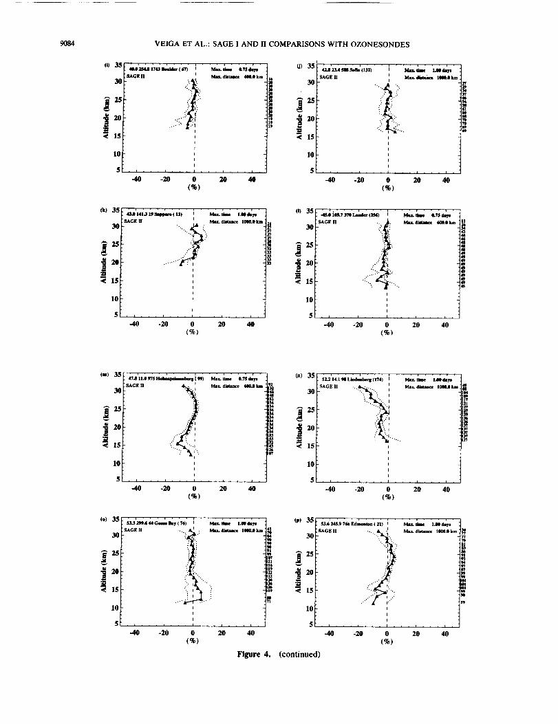
Figure 4. Median difference profiles for the ensemble of ozonesonde/SAGE II paired data. See Table 1for the applicable dates. The units are in percentage relative to SAGE II. The dotted band represents the95% confidence interval of the median difference. Only confidence intervals whose length is less than 20%are shown. Samples sizes at each altitude are marked along the right axis. Figure 4v is a compilation of thefrequency with which the combined ozonesonde/satellite differences were less than 5%. Each open barrepresents the total number of sample differences available for a given altitude, and the shaded bar is thenumber of sample differences less than 5%.
9084 VEIGA ET AL.: SAGE I AND II COMPARISONS WITH OZONESONDES
o) 35
3O
_ 20
10
5
ZSAGE n
• k-
_:_
-410 -20
Mare dlmaee ¢,N.O tom
, , . i . . . i .
0 2O 4O
(%)
(J) 35
2, 30
UmloN3o1, _ 2019n9 ._
10
i SAGE II t MmL diMmme 1000.0 kmI
• i . . . t . . . t . . . t . . . 1 ,
-40 -20 0 20 40
(%)
(k) 3_ t d_L0'14|'.319_¢e'(12) " ; MaLt_ "lJO_." :
_SAGE H i MmL d_tsace IMI0.0 km i
"'"I "-
j 20 ........
< 15[
lO_-5F......... : .........
-40 -20 0 20 40
(%)
(t) 35
30
_ 2s
_ 20
10
5
• i • ...... ; M_tk. ,..d_,
SAGE II "i_"_'#:[i':'- MImL dlkdmtee 60e.O laa
"::_iI ....
I
I
I
I
-40 -20 0 20 40(%)
(m) 35
3O
25
l0
Co) 35
30
20
15
10
5
....•"7i..: : I
I
I
I
• , - - - , , , , I , , , I , , , 1 ,
-40 -20 0 20 40
(%)
(n) 35
30
_ 20
lO
: SAGE 1, .._.. : Minx. dl_am_ lON.O km•. . _
:j -'_
I
I
I
I
I
L
-40 -20 0 20 40
(%)
," " M", I, 9_
• : I1
" .1" 19: ., _[2• ", 22
". I : 19
-40 -20 0 20 40
(%)
(p) 35
30
25
15
10
SAGE II ..,...'_ MtLv_ dilute 10N.O km
-.. ':
,5 :_.//'
I
I
I
-40 -20 0 20 40
(%)
Figure 4. (continued)
1721
lY/
01

VEIGA ET AL.: SAGE I AND II COMPARISONS WITH OZONESONDES 9085
(q) 35
30
2s
10
5
(.) 35
30
25
20
15
10
I
.ii .... .:
...'"" "1
I
I
I
I
• i . , . i , . , I . • . , • • , l •
-40 -20 0 20 40(%)
(r) 35
3O
25
20
l0
5
SAGE II I Mu. dltn_ Ill00,0 Iluu
,.. ...i..'1
'J • ";:,
'.. "'p....
i
I
-40 .20 0 20 40(%)
_$AGE H I. 4_.., Max. di_ance 14iOOJPkm'. ..""
)" '1..
..' ..J'
I
I
-40 -20 0 20 40(%)
(t) 35
3O
2s_ 2o
10
5
• . - • • i - - - , - - - , - • • i •
-69.0 39,6 21 Syows (101) I Max. time 2.00 daysi
:.. t:
... • "I
""... "".1
"".. :-A
I
I
I
-40 -20 0 20 40(%)
(u> 35
30
15
10
,II
I
I
-40 -20 0 20 40(%)
Figure 4.
(v) 35
186_77?"t788S
8.5
9t
" i91
;tS8836a
10
5
0
(continued)
5 10 15 20
Number of Differences < 5 %
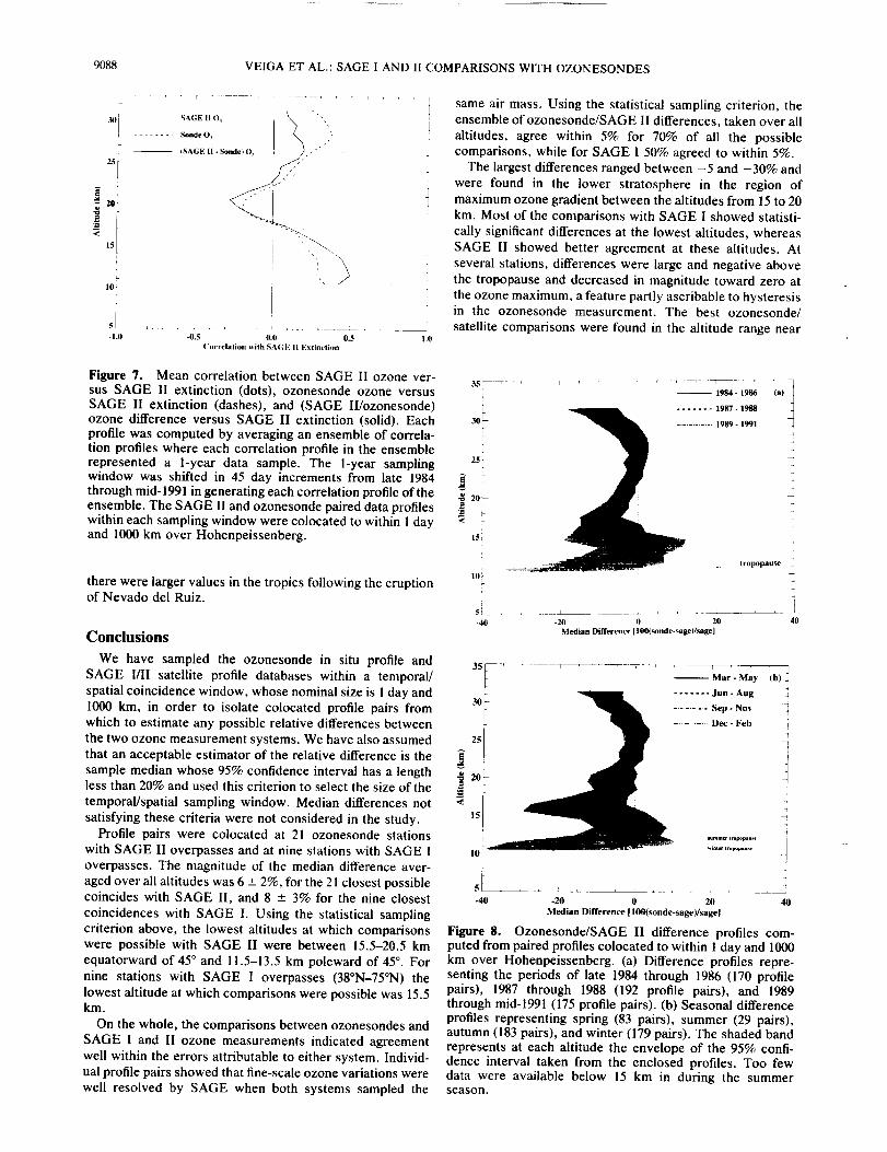
of correlation profiles of SAGE II/ozonesonde ozone differ-ence versus extinction (note this is the negative of the
correlation profile discussed above). It would be expected
that if the satellite and ozonesonde agreed exactly, or if theirdifference were random, the correlation profile would be
zero. The vertical structure in the SAGE II/ozones0nde
difference versus extinction correlation indicates the exis-
tence of a residual bias between the two ozone measurement
systems, or an ozone retrieval effect, or an intrinsic property
of the vertical structure of the stratosphere. To show evi-dence for the latter, the correlation between the SAGE II
ozone and SAGE II extinction for the paired data sampling
over Hohenpeissenberg is shown in Figure 7 as the dotted
curve, and similarly the dashed curve is the correlationbetween ozonesonde ozone and SAGE II extinction_
Clearly, both these correlation profiles have an almost
identical vertical structure although the magnitudes differ.Since the sonde ozone is a measurement independent from
the SAGE II extinction, the vertical structure of the corre-lation of SAGE II ozone and SAGE II extinction cannot be
due solely to satellite ozone retrieval aerosol effects. The
differences in magnitudes between the dashed and dotted
curves can be explained by the fact that the ozonesonde
measurements are not exactly colocated in time and space
with the satellite extinction measurements, and hence the
ozonesonde versus extinction correlation is always less in
magnitude than the satellite ozone versus satellite extinction
correlation. Cunnold and Veiga [1991] proposed that the
vertical structure of the correlation between ozone and
extinction is produced by horizontal and vertical advection
of the constituents.
The ozonesonde/SAGE II difference profiles computed

9086 VEIGAET AL.: SAGE I AND II COMPARISONS WITH OZONESONDES
(,) 35
3O
25
•¢ 15
10
37.8 18d.$13 W_ _ (1_)
SAGE I " •": _-_t
. . .S ['"
Mu. dl_nc¢ tO0_O k_m
(b) 35
30
25
15
10
g
: _('3_iSBbatnmnm(197) ; " "Mu._bu_ "_D0da_u"
.-" I
.." "I
....'
-40 -20 0 20 40 -40 -20 0 20 40(%) (%)
[SAGE ! .. ,it,.. I Mex. dimuee INOJI km
- ;._
_20 -" :" _• ;I I
,o[5/, I , , , i , , , i
-40 -20 0 20 40(%)
(d) 35
30
20
10
5
• , • . . , . . . , . . . , . . . ) •
4%5 !1.1 ?40,ff_ (_1_ ))SAGE I
• . • i
"'F.
MbL tbie I,,N do35
Max. dbmmce 1000JP km
• i . . . i . , , i , , , l . . . i .
-40 -20 0 20 40(%)
(e) 35
3O
| 20i
1o
5
'.. '.'.
i) :,)...." .' I
)
t
I
)
t
-40 -20 0 20 40(%)
35 t ._3.3'_._"c_,,_,,(7g i " u,,._ "_._d_-30 , ..)
20 9 !:
15 I10
-40 -20 0 20 40(%)
(_ 35
30
25
20•_ 15
10
• . • - • , - - . i • . . ) ....• %6 2_.9 ?_ F_tmemlom ( 21 ) I ]MhtL time 1.00 ,a-'y_
SAGE i I _ dimanee 1000.0 km• -. .L.
t
I
I
)
I
-40 -20 0 20 40
(%)
(b) 35[ _'_#'c_hm(_)" ; " M_,._,,_ ",.O0d_y," 1[ SAGE I ) Mm_ d_mm_¢ I_.0 km ]tl
"I ....' 1• " "'.1 14
_ I,'
• ""I ". 18
". 18
20 _0• • ]8
.,* tit
• "f t5L ......... , .........
-40 -20 0 20 40(%)
Figure 5. Median difference profiles for the ensemble of ozonesonde/SAGE I paired data. See Table 1for the applicable dates. The units are in percentage relative to SAGE I. The dotted band represents the95% confidence interval of the median difference. Only confidence intervals whose length is less than 20%are shown. Sample sizes at each altitude are marked along the rightaxis. Figure 5j is the same as in Figure4v.

VEIGA ET AL.: SAGE I AND I1 COMPARISONS WITH OZONESONDES 9087
(. 35
30
25
_ 20
10
sl
- f " . - , • - - , . . • i - • • , .
74.7 26$.0 64 _ate _ 24) I Max. tbae 2.llO drays
_ SAGE l ......... '"'.."'__.. ' !.MMx. d.net.';!:" "'.. t"" "P'..";'"["'r:'( '"",. l..O km
t
i
t
I
• t . . . 1 , , , 1 , , , A , . , i ,
-40 .20 0 20 40(%)
_1) 35
s 30
25
lO
5
' AE• . . i • . • L
2 4 6 8
Number of Differences < 5 %
Figure 5. (continued)
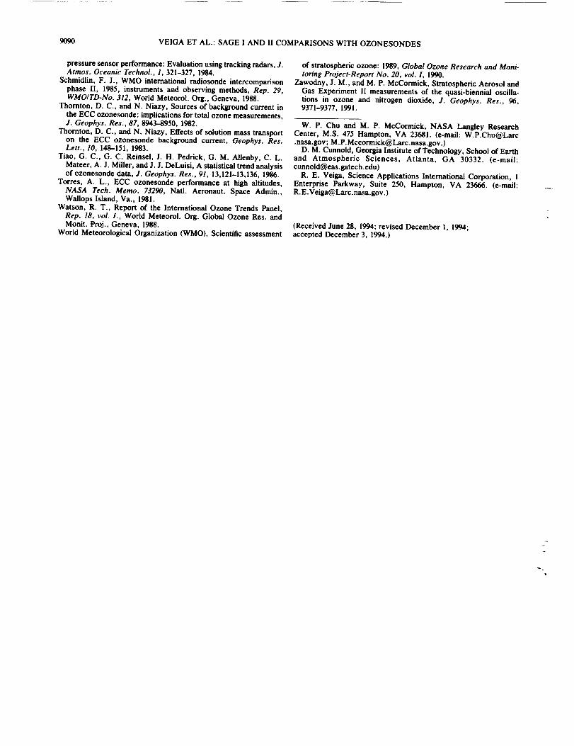
during varying aerosol conditions and seasons are shown in
Figure 8. Figure 8a shows the difference profiles computedfor three periods ranging from high to low aerosol extinction
levels. The shaded band is the envelope of the 95% confi-
dence interval at each altitude. The differences between any
pair of the three profiles shown were not significant at any
altitude, and hence these results indicate that the relativedifference between the SAGE II ozone measurements and
the ozonesondes over Hohenpeissenberg were temporally
constant. Figure 8b shows the difference profiles from sea-
sonal sampling of the period from late 1984 through mid-
1991. Occultation sampling allowed the most overpasses
during the fall and winter, while the summer months were
sampled less frequently, and consequently little data were
available below 15 km during the June through August time
period. The seasonal variation of the mean tropopause isshown by the tropopause altitudes during winter and sum-
mer at this location. Since the 95% confidence intervals for
any given pair of difference profiles overlapped, these data
indicate that there were no significant seasonal biases in the
ozonesonde/SAGE II difference.
It must be emphasized that the results above are derived
from analyzing the data over the midlatitudes between 1984
and mid-1991, and that possible aerosol/ozone correlations
in the SAGE II data may exist at other latitudes. Analysis of
the SAGE II data after the eruption of Mount Pinatubo
indicates that the ozone is not correlated with aerosol
extinction whenever the 1 /xm extinction is less than 0.001km -] . While the midlatitudes never attained extinction
values larger than this prior to the Mount Pinatubo eruption,
;:
_ :":
•L. "i
:!j....i . 'p
!" I: • " .'."
"" ":"'-" i:.lll! ! :-e itl!:li :
ii "- '!: : ':; '! '-•....
• ",! "i , I: i " I i" i_ll'i I
1984 1986 1988 1990
Figure 6. SAGE II 1020 nm extinction at 18.5 km over the latitude band extending from 43°N to 53°N.
9088 VE1GAETAL.:SAGEI ANDII COMPARISONSWITHOZONESONDES
- - - Sonde O, ',
-- (SAGE I1 - Sonde) O
-,5fj _
?
!01 " _
- 1.0 -0.5 0.0 0.5 1.0
Correlation wilh SAGE I1 Extinction
same air mass. Using the statistical sampling criterion, the
ensemble of ozonesonde/SAGE II differences, taken over all
altitudes, agree within 5% for 70% of all the possible
comparisons, while for SAGE I 50% agreed to within 5%.
The largest differences ranged between -5 and -30% and
were found in the lower stratosphere in the region of
maximum ozone gradient between the altitudes from 15 to 20
km. Most of the comparisons with SAGE I showed statisti-
cally significant differences at the lowest altitudes, whereas
SAGE II showed better agreement at these altitudes. At
several stations, differences were large and negative above
the tropopause and decreased in magnitude toward zero at
the ozone maximum, a feature partly ascribable to hysteresis
in the ozonesonde measurement. The best ozonesonde/
satellite comparisons were found in the altitude range near
Figure 7. Mean correlation between SAGE II ozone ver-
sus SAGE II extinction (dots), ozonesonde ozone versus
SAGE II extinction (dashes), and (SAGE II/ozonesonde)
ozone difference versus SAGE II extinction (solid). Each
profile was computed by averaging an ensemble of correla-
tion profiles where each correlation profile in the ensemble
represented a 1-year data sample. The l-year samplingwindow was shifted in 45 day increments from late 1984
through mid-1991 in generating each correlation profile of the
ensemble. The SAGE II and ozonesonde paired data profiles
within each sampling window were colocated to within i dayand 1000 km over Hohenpeissenberg.
there were larger values in the tropics following the eruptionof Nevado del Ruiz.
Conclusions
We have sampled the ozonesonde in situ profile and
SAGE I/II satellite profile databases within a temporal/
spatial coincidence window, whose nominal size is l day and
1000 km, in order to isolate colocated profile pairs from
which to estimate any possible relative differences between
the two ozone measurement systems. We have also assumed
that an acceptable estimator of the relative difference is the
sample median whose 95% confidence interval has a length
less than 20% and used this criterion to select the size of the
temporal/spatial sampling window. Median differences not
satisfying these criteria were not considered in the study.
Profile pairs were colocated at 21 ozonesonde stations
with SAGE II overpasses and at nine stations with SAGE !
overpasses. The magnitude of the median difference aver-
aged over all altitudes was 6 -+ 2%, for the 21 closest possible
coincides with SAGE II, and 8 -+ 3% for the nine closest
coincidences with SAGE I. Using the statistical sampling
criterion above, the lowest altitudes at which comparisons
were possible with SAGE II were between 15.5-20.5 km
equatorward of 45 ° and 11.5-13.5 km poleward of 45 °. For
nine stations with SAGE I overpasses (38°N-75°N) the
lowest altitude at which comparisons were possible was 15.5km.
On the whole, the comparisons between ozonesondes and
SAGE I and II ozone measurements indicated agreement
well within the errors attributable to either system. Individ-
ual profile pairs showed that fine-scale ozone variations were
well resolved by SAGE when both systems sampled the
J
35 -- _ r
lo!
5_-40
__ tropopause
-20 0 20
Median Difference [ 100(sonde-sage)/sage]
35(r _-_ • i t
-- Mar-May (b)
L ....... Jun - Aug30
_- ........... Sep - Nov
............ Dec - Feb4
,L
J40
-40 -20 0 20 40
Median Difference 1100(sonde-sage)/sagel
Figure 8. Ozonesonde/SAGE II difference profiles com-puted from paired profiles colocated to within 1 day and 1000km over Hohenpeissenberg. (a) Difference profiles repre-senting the periods of late 1984 through 1986 (170 profilepairs), 1987 through 1988 (192 profile pairs), and 1989through mid-1991 (175 profile pairs). (b) Seasonal differenceprofiles representing spring (83 pairs), summer (29 pairs),autumn (183 pairs), and winter (179 pairs). The shaded band
represents at each altitude the envelope of the 95% confi-dence interval taken from the enclosed profiles. Too fewdata were available below 15 km in during the summerseason.

VEIGAETAL.:SAGEI AND II COMPARISONS WITH OZONESONDES 9089
the ozone maximum (21-26 km), where essentially all com-
parisons showed differences less than 5%.
The selection of the ozone profile pairs based solely on a
specific temporal/spatial sampling window (up to 2 days and
1000 km) inevitably includes a relatively large number of
cases where the paired profiles represented different synop-
tic conditions. As a consequence the large sizes of the 95%
confidence intervals at lower stratospheric levels shown in
Figures 4, 5, and 8 contain a geophysical component. One
method of accounting for the synoptic component is to use a
back-trajectory analysis to properly compare ozone mea-
surements from similar air masses. This would probably
improve the confidence in the lower stratospheric compari-
sons.
Analysis of the correlation between aerosol extinction and
ozonesonde/SAGE II differences at one northern midlatitude
station revealed that the SAGE II ozone retrieval was not
affected by the levels of aerosol encountered in the lower
stratosphere in the time period between late 1984 and
mid-1991. A temporally invariant vertical structure in the
correlation profile between ozone and extinction appears in
both the SAGE II ozone data and in the ozonesonde data and
is possibly indicative of transport processes in the strato-
sphere. During the time period from late 1984 through
mid-1991 the ozonesonde/SAGE II difference profile showed
insignificant changes in the lower stratosphere (below 20 km)
as the extinction varied by an order of magnitude throughout
the period. No significant seasonal biases in the difference
profiles were detected.
Acknowledgments. We thank S. J. Oltmans for providing theHilo, Samoa, and Boulder ozonesonde data; W. A. Matthews forproviding the Lauder ozonesonde data; D. De Muer for providingthe SAGE II and Uccle comparison profiles; C. Trepte, and J.Zawodny for valuable discussions. R. Veiga was supported byNASA contract (NAS1-19570). D. M. Cunnold was supported byNASA contract (NAS1-19954).
References
Attmannspacher, W., J. de la Noe, D. de Muer, J. Lenoble, G.Megie, J. Pelon, P. Pruvost, and R. Reiter, European validation ofSAGE II ozone profiles, J. Geophys. Res., 94, 8461--8466, 1989.
Barnes, R. A., A. R. Bandy, and A. L. Torres, Electrochemicalconcentration cell ozonesonde accuracy and precision, J. Geo-phys. Res., 90, 7881-7887, 1985.
Barnes, R. A., L. R. McMaster, W. P. Chu, M. P. McCormick, andM. E. Gelman, Stratospheric Aerosol and Gas Experiment II andROCOZ-A ozone profiles at Natal, Brazil: A basis for comparisonwith other satellite instruments, J. Geophys. Res., 96, 7515-7530,1991.
Bass, A. M., and R. J. Paur, The ultraviolet cross-sections of ozone,I, The measurements, in Atmospheric Ozone, Proceedings of theInternational Quadrennial Ozone Symposium, Halkidiki, Greece,edited by C. Zerefos and A. Ghazi, pp. 606--616, D. Reidel,Hingham, Mass., 1985.
Brewer, A. W., and J. R. Milford, The Oxford-Kew Ozone sonde,Proc. R, Soc. London, A256, 470--495, 1960.
Chu, W., and M. P. McCormick, Inversion of stratospheric aerosoland gaseous constituents from spacecraft solar extinction data inthe 0.38-1.0 _m wavelength region, Appl. Opt., 18, 1404--1414,1979.
Chu, W. P., M. P. McCormick, J. Lenoble, C. Brogniez, and P.Pruvost, SAGE I1 inversion algorithm, J. Geophys. Res., 94,8339-8351, 1989.
Cunnold, D. M., and R. E. Veiga, Preliminary assessment ofpossible aerosol contamination effects on SAGE ozone trends inthe lower stratosphere, Adv. Space Res., 11(3)5-3(8), 1991.
Cunnold, D. M., W. P. Chu, R. A. Barnes, M. P. McCormick, and
R. E. Veiga, Validation of SAGE I1 ozone measurements, J.Geophys. Res., 94, 8447-8460, 1989.
De Muer, D,, and H. Malcorps, The frequency response of an
electrochemical ozone sonde and its application to the deconvo-lution of ozone profiles, J. Geophys. Res., 89, 1361-1372, 1984.
De Muer, D., H. De Backer, R. E. Veiga, and J. M. Zawodny,Comparison of SAGE II ozone measurements and ozone sound-
ings at Uccle (Belgium) during the period February 1985 toJanuary 1986, J. Geophys. Res., 95, 11,903-11,911, 1990.
Efron, B., The Jacknife, the Bootstrap, and Other ResamplingPlans, Society for Industrial and Applied Mathematics, Philadel-
phia, Pa., 1982.Harder, J. W,, Measurements of springtime antarctic ozone deple-
tion and development of a balloonborne ultraviolet photometer,Ph.D. thesis, Univ. of Wyoming, Phys. and Astron. Dept.,
Laramie, Wyo., 1987.Hilsenrath, E., et al., Results from the balloon ozone intercompar-
ison campaign, J. Geophys. Res., 91, 13,137-13,152, 1986.Komhyr, W. D., A carbon-iodine sonde sensor for atmospheric
soundings, Proc. Ozone Syrup., Albuquerque, p. 26, Geneva,1965.
Komhyr, W. D., Electrochemical concentration cells for gas analy-sis, Ann. Geophys., 25, 203-210, 1969.
Komhyr, W. D., Dobson spectrophotometer systematic total ozonemeasurement error, Geophys. Res. Left., 7, 161-163, 1980.
Komhyr, W. D., and T. W. Harris, Note on flow rate measurementsmade on Mast-Brewer ozone sensor pumps, Mon. Weather Rev.,93,267-268, 1965.
Komhyr, W. D., and T. B. Harris, Development of an ECC
ozonesonde, NOAA Tech. rep. ERL 200-APCLI8, U.S. Dep.Commer., Boulder, Colo., 1971.
Komhyr, W. D., J. D. Lathrop, D. P. Opperman, R. A. Barnes, andG. B. Brothers, ECC ozonesonde performance evaluation during
STOIC 1989, J. Geophys. Res., in press, 1994.List, R. J., Smithsonian Meteorological Tables, Smithsonian Insti-
tution, Washington, D.C., 1951.Logan, J. A., Tropospheric ozone: Seasonal behavior, trends, and
anthropogenic influence, J. Geophys. Res., 90, 10,463-10,482,1985.
Margitan, J. J., et al., lntercomparison of ozone measurements overAntarctica, J. Geophys. Res., 94, 16,557-16,569, 1989.
Mauldin, L. E., N. H. Zaun, M. P. McCormick, J. H. Guy, andW. R. Vaughn, Stratospheric Aerosol and Gas Experiment IIinstrument: A functional description, Opt. Eng., 24(2), 307-312,1985.
McCormick, M. P., and R. Reiter, SAGE-European ozonesondecomparison, Nature, 300, 337-339, 1982.
McCormick, M. P., and J. C. Larsen, Antarctic measurements ofozone by SAGE II in the spring of 1985, 1986, and 1987, Geophys.Res. Lett., 15,907-910, 1988.
McCormick, M. P., and R. E. Veiga, SAGE I! measurements of
early Pinatubo aerosols, Geophys. Res. Lett., 19, 155-158, 1992.McCormick, M. P., P. Hamill, T. J. Pepin, W. P. Chu, T. J.
Swissler, and L. R. McMaster, Satellite studies of the strato-spheric aerosol, Bull. Am. Meteorol. Soc., 60(9), 1038-1046, 1979.
McCormick, M. P., T. J. Swissler, E. Hilsenrath, A. J, Krueger, andM. T. Osborn, Satellite and correlative measurements of strato-spheric ozone: Comparison of measurements made by SAGE,ECC balloons, chemiluminescent, and optical rocketsondes, J.Geophys. Res., 89, 5315-5320, 1984.
McCormick, M. P., R. E. Veiga, and J. M. Zawodny, Comparisonof SAGE I and SAGE II stratospheric ozone measurements, inOzone in the Atmosphere, edited by R. D. Bojkov and P. Fabian,202-205, A. Deepak, Hampton, Va., 1989a.
McCormick, M. P., J. M. Zawodny, R. E. Veiga, J. C. Larsen, andP. H. Wang, An overview of SAGE I and SAGE I1 ozonemeasurements, Planet. Space Sci., 12, 1567-1586, 1989b.
McCormick, M. P., R. E. Veiga, and W. P. Chu, Stratospheric
ozone profile and total ozone trends derived from the SAGE I andSAGE II data, Geophys. Res. Lett., 19, 269-272, 1992.
McDermid, I. S., et al., Comparison of ozone profiles from ground-based Lidar, electrochemical concentration cell balloon sonde,ROCOZ-A rocket ozonesonde, and Stratospheric Aerosol andGas Experiment satellite measurements, J. Geophys. Res., 95,10,037-10,042, 1990.
Parsons, C. L., G. A. Norcross, and R. L. Brooks, Radiosonde
9090 VEIGAETAL.:SAGE I AND II COMPARISONS WITH OZONESONDES
pressure sensor performance: Evaluation using tracking radars, J.Atmos. Oceanic Technol., 1,321-327, 1984.
Schmidlin, F. J., WMO international radiosonde intercomparisonphase II, 1985, instruments and observing methods, Rep. 29,WMO/TD-No. 312, World Meteorol. Org., Geneva, 1988.
Thornton, D. C., and N. Niazy, Sources of background current inthe ECC ozonesonde: implications for total ozone measurements,J. Geophys. Res., 87, 8943-8950, 1982.
Thornton, D. C., and N. Niazy, Effects of solution mass transporton the ECC ozonesonde background current, Geophys. Res.Lett., 10, 148-151, 1983.
Tiao, G. C., G. C. Reinsel, J. H. Pedrick, G. M. Allenby, C. L.Mateer, A. J. Miller, and J. J. DeLuisi, A statistical trend analysisof ozonesonde data, J. Geophys. Res., 91, 13,121-13,136, 1986.
Tones, A. L., ECC ozonesonde performance at high altitudes,NASA Tech. Memo. 73290, Natl. Aeronaut. Space Admin.,Wallops Island, Va., 1981.
Watson, R. T., Report of the International Ozone Trends Panel,Rep. 18, vol. 1., World Meteorol. Org. Global Ozone Res. andMonit. Proj., Geneva, 1988.
World Meteorological Organization (WMO), Scientific assessment
of stratospheric ozone: 1989, Global Ozone Research and Moni-toring Project-Report No. 20, vol. I, 1990.
Zawodny, J. M., and M. P. McCormick, Stratospheric Aerosol andGas Experiment 1I measurements of the quasi-biennial oscilla-tions in ozone and nitrogen dioxide, J. Geophys. Res., 96,9371-9377, 1991.
W. P. Chu and M. P. McCormick, NASA Langley ResearchCenter, M.S. 475 Hampton, VA 23681. (e-mail: [email protected]; M.P. Mccormick@ Larc. nasa.gov.)
D. M. Cunnoid, Georgia Institute of Technology, School of Earthand Atmospheric Sciences, Atlanta, GA 30332. (e-mail:[email protected])
R. E. Veiga, Science Applications International Corporation, IEnterprise Parkway, Suite 250, Hampton, VA 23666. (e-mail:[email protected].)
(Received June 28, 1994; revised December I, 1994;accepted December 3, 1994.)
Recommended