Jeroen TrompMin Chen, Vala Hjorleifsdottir, Dimitri Komatitsch, Swami Krishnan, Qinya Liu,
Alessia Maggi, Anne Sieminski, Carl Tape & Ying Zhou
Spectral-Element and Adjoint Methods in Seismology

Introduction to the Spectral-Element Method(SEM)

Governing Equations
Equation of motion:
Boundary condition:
Initial conditions:
Earthquake source:

Weak Form
• Weak form valid for any test vector• Boundary conditions automatically included• Source term explicitly integrated
Finite-fault (kinematic) rupture:

Finite-Elements
Mapping from reference cube to hexahedral elements:
Volume relationship:
Jacobian of the mapping:
Jacobian matrix:

Lagrange Polynomials and Gauss-Lobatto-Legendre (GLL) Points
Degree 4 GLL points:
GLL points are n+1 roots of:
The 5 degree 4 Lagrange polynomials:
Note that at a GLL point:
General definition:
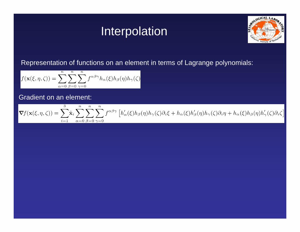
Interpolation
Representation of functions on an element in terms of Lagrange polynomials:
Gradient on an element:

Integration
Integration of functions over an element based upon GLL quadrature:
• Integrations are pulled back to the reference cube• In the SEM one uses:
• interpolation on GLL points• GLL quadrature
Degree 4 GLL points:
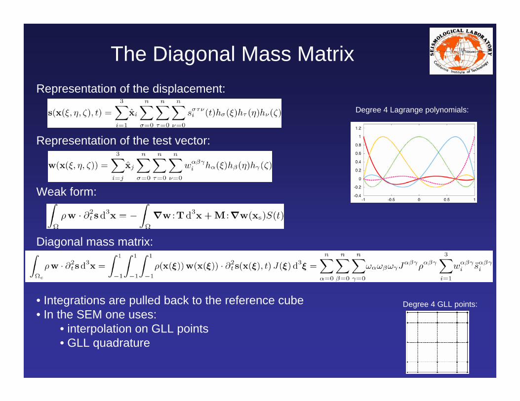
The Diagonal Mass MatrixRepresentation of the displacement:
Representation of the test vector:
Weak form:
Diagonal mass matrix:
• Integrations are pulled back to the reference cube• In the SEM one uses:
• interpolation on GLL points• GLL quadrature
Degree 4 Lagrange polynomials:
Degree 4 GLL points:

Assembly
Global equations:
Need to distinguish:• local mesh• global mesh
Efficient routines available from FEM applications
Global SEM time-marching is based upon an explicit second-order time scheme

Parallel Implementation
Global mesh partitioning:
Cubed Sphere: 6 n mesh slices2
Regional mesh partitioning:
n x m mesh slices

Basin Code: SPECFEM3D_BASIN
• Freely available for non-commercial use from geodynamics.org• Manual available at geodynamics.org• 3D Attenuation• 3D Anisotropy• Ocean load• Topography & bathymetry• Kinematic ruptures• Movies• Models:
– Harvard 3D Southern California model– SOCAL 1D model– Homogeneous half-space model
• Adjoint capabilities

Southern California Simulations
-30
-20
-10
0
10
0 50 100 150 200 250 300 350 400
2 3 4 5 6 7 8Vp(km/s)
B B’
-30
-20
-10
0
10
0 50 100 150 200 250 300 350 400 450
A A’
n x m mesh slices
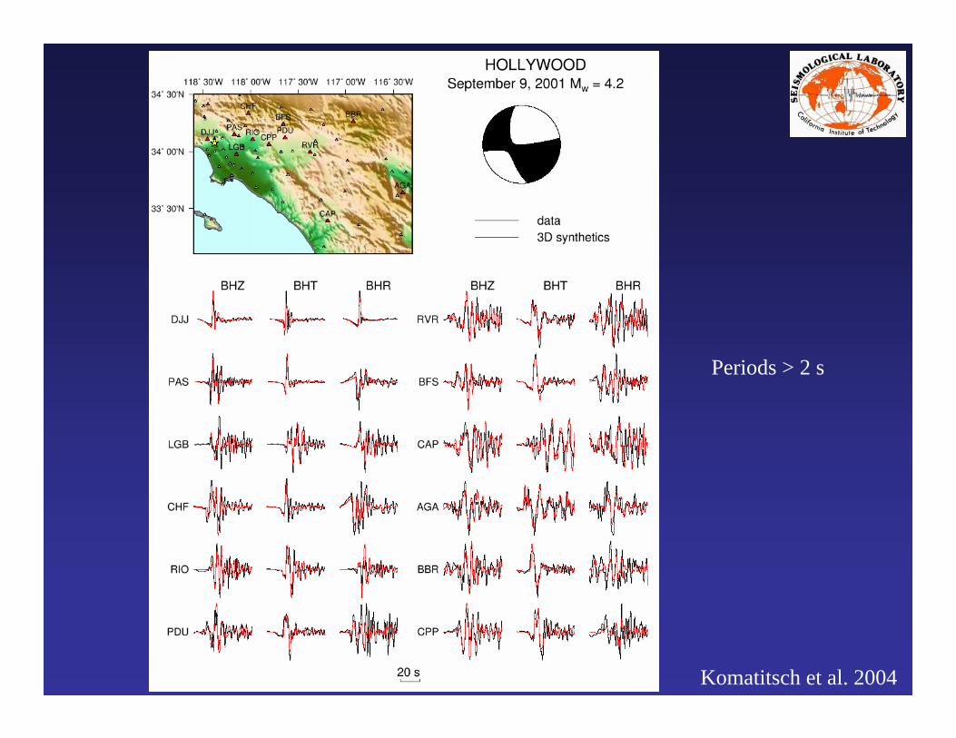
Periods > 2 s
Komatitsch et al. 2004
June 12, 2005, M=5.1 Big Bear
QuickTime™ and aYUV420 codec decompressor
are needed to see this picture.

100km
379 k
m
3D Regional Forward Simulations
Qinya Liu
June 12, 2005, M=5.1 Big Bear
Periods > 6 s

San Andreas Rupture Scenario
QuickTime™ and aYUV420 codec decompressor
are needed to see this picture.

San Andreas Rupture Scenario:Quantitative Seismic Hazard Assessment
Swami Krishnan

Near Real-Time Applications• Automated near real-time simulations of all M>3.5 events• ShakeMovies at http://www.shakemovie.caltech.edu/• Soon:
– CMT solutions– Synthetic seismograms

SPECFEM3D_BASIN: Future Plans
• Switch to a (parallel) CUBIT hexahedral finite-element mesher (Casarotti, Lee)– Topography & bathymetry– Major geological interfaces– Basins– Fault surfaces
• Use ParMETIS or SCOTCH for mesh partitioning & load-balancing• Retain the SPECFEM3D_BASIN solver (takes ParMETIS meshes; Komatitsch)• Add dynamic rupture capabilities (Ampuero, Lapusta, Kaneko)
100km
102km
88km
Taipei Basin N
S.-J. Lee

Global Code: SPECFEM3D_GLOBE
• Freely available for non-commercial use from geodynamics.org• Manual available at geodynamics.org• 3D Attenuation• 3D Anisotropy• Ocean load• Topography & bathymetry• Rotation• Self-gravitation (Cowling approximation)• Kinematic ruptures• Movies• Models:
– 1D models: isotropic PREM, transversely isotropic PREM, AK135, IASP91, 1066A– S20RTS– Crust2.0
• Adjoint capabilities

Global Simulations
PREM benchmarks Cubed sphere mesh
Parallel implementation:6 n mesh slices2

SEM Implementation of Attenuation
Modulus defect:
Unrelaxed modulus:
Memory variable equation:
Equivalent Standard Linear Solid (SLS) formulation:
Anelastic, anisotropic constitutive relationship:
Attenuation (3 Attenuation (3 SLSsSLSs))
Physical dispersion (3 Physical dispersion (3 SLSsSLSs))

Effect of Attenuation

Attenuation

Effect of Anisotropy

SEM Implementation of Anisotropy

Antipodal Transverse Record
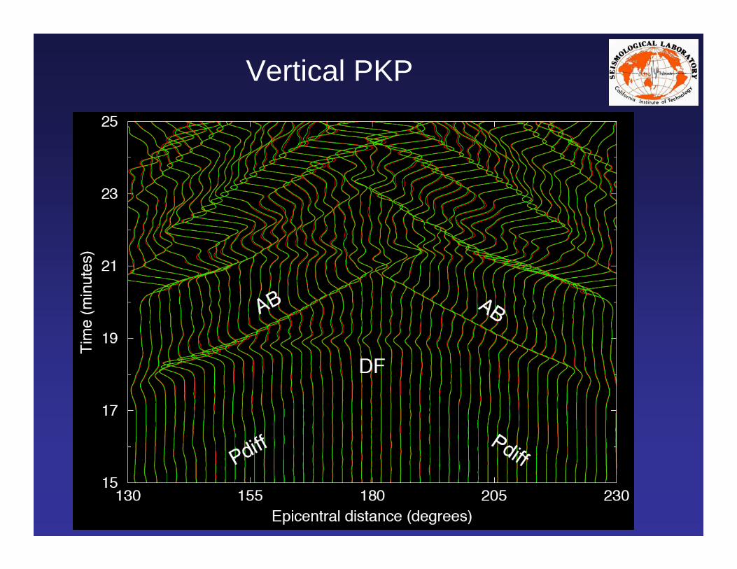
Vertical PKP

Rotation & Self-Gravitation
Wave equation solved by SPECFEM3D_GLOBE in crust, mantle and inner core:
Wave equation solved by SPECFEM3D_GLOBE in fluid outer core:
SPECFEM3D_GLOBE uses domain decomposition between the fluid outer core and the solid inner core and mantle matching exactly:• continuity of traction• continuity of the normal component of displacement

Full Gravity Versus Cowling

SEM Implementation of Gravity

Effect of Ocean

SEM Implementation of Ocean
Modified boundary condition:

3D Mantle Models
S20RTS (Ritsema et al. 1999)

Crustal and Topographic Models
Crust 2.0 (Bassin et al. 2000) ETOPO5

Great 2004 Sumatra-Andaman Earthquake
Main shock & aftershocks (Harvard)
Finite slip model (Chen et al., 2005)

Sumatra Surface Waves
QuickTime™ and aYUV420 codec decompressor
are needed to see this picture.

Surface-Wave Fits
Vala Hjorleifsdottir

SPECFEM3D_GLOBE: Future PlansOn-demand TeraGrid applications:• Automated, near real-time simulations of all M>6 earthquakes• Analysis of past events (more than 20,000 events)• Seismology Web Portal (prototype available at this meeting)
Petascale simulations:• Global simulations at 1-2 Hz• New doubling brick
(perfect load-balancing)

Adjoint Spectral-Element Simulations(ASEM)

Adjoint Tomography
PDE-constrained waveform tomography:
Change in the waveform misfit function:

Adjoint Equations
Adjoint wavefield:
Adjoint equation of motion:
Adjoint boundary conditions:
Adjoint initial conditions:
Adjoint source:
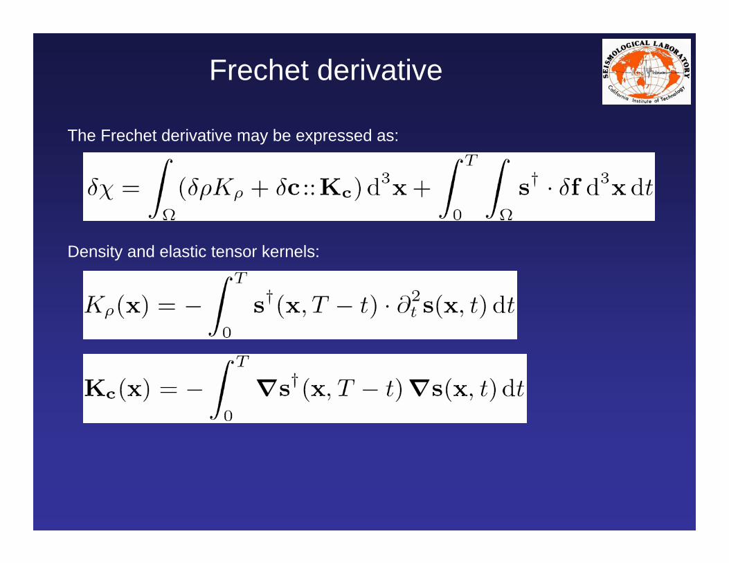
Frechet derivative
The Frechet derivative may be expressed as:
Density and elastic tensor kernels:

Isotropic KernelsFor isotropic perturbations we have:
where
and we have defined the strain deviators
In terms of wave speeds:
where

Traveltime Frechet DerivativesTraveltime tomography:
Change in the misfit function:
Traveltime anomaly in terms of banana-donut kernel (Dahlen):
The kernel is a weighted sum of banana-donut kernels :

Adjoint Wavefield
Kernel in terms of the adjoint wavefield:
The adjoint wavefield is generated by the adjoint source
Notes:• Need simultaneous access to the regular wavefield at time t and the adjoint wavefield at time T – t• Use of the time-reversed velocity as the source for the adjoint wavefield

Need simultaneous access to and• During calculation of adjoint field ,
reconstruct by solving the `backward’ wave equationNeed to store from a previous forward simulation:– Last snapshot– Wavefield absorb on artificial boundariesChallenge:– `Undoing’ attenuation
Numerical Implementation

2D Adjoint Tomography

Construction of a Banana-Donut Kernel
Tape et al. 2006

Adjoint Tomography

Construction of an Event Kernel
Event Kernel:
• Sum of weighted banana-donut kernels
• Two simulations per event

Construction of the Misfit Kernel
Misfit kernel:
• Sum of all the event kernels• Two simulations per event• Gradient of misfit function

Conjugate Gradient Algorithm

Conjugate Gradient Algorithm
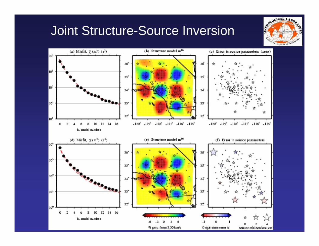
Joint Structure-Source Inversion


Southern California Rayleigh Waves
25 events

Toward 3D Tomography: SPECFEM3D Adjoint Capabilities

3D Sensitivity Kernels
Liu & Tromp 2006
S
PS PS
SS
SPECFEM3D_BASIN
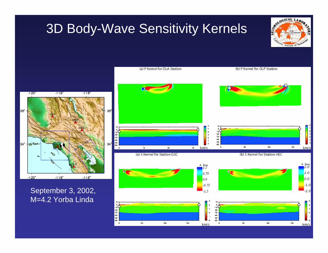
3D Body-Wave Sensitivity Kernels
September 3, 2002,M=4.2 Yorba Linda

3D Surface-Wave Sensitivity KernelsRayleigh (HEC)
Love (HEC)

Our First 3D Event Kernels!

Qinya Liu
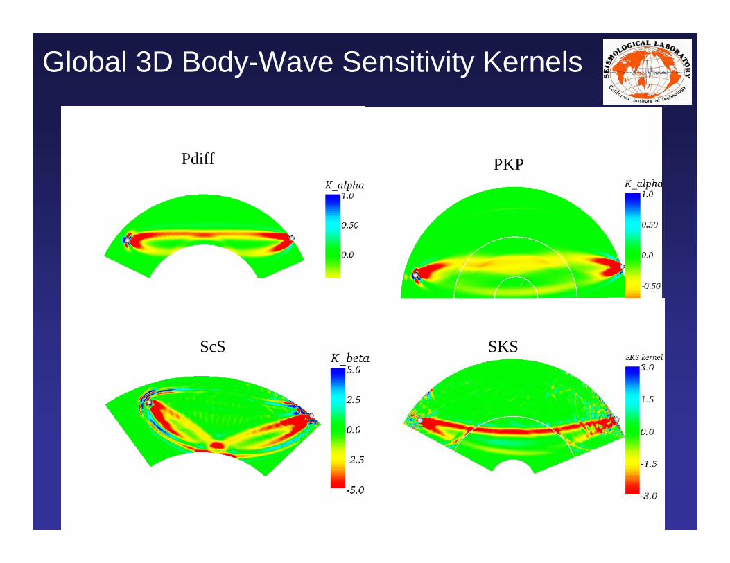
Global 3D Body-Wave Sensitivity Kernels
SPECFEM3D_GLOBE
20 second P wave9 second P wave
Finite-Frequency effects
Qinya Liu
Global 3D Body-Wave Sensitivity Kernels
Pdiff
ScS
PKP
SKS

PKP Kernel

P’P’ Kernel
Liu & Tromp 2006

α
η
α
β β
ρ
h
h
v
v
Anne Sieminski
α
η
α
β β
ρ
h
h
v
v
P SH
Global 3D Transversely Isotropic Kernels

Anne Sieminski
Transversely IsotropicParameters: A, C, L, N, F1 ζ: J, K, M2 ζ: G, B, H3 ζ: D4 ζ: E
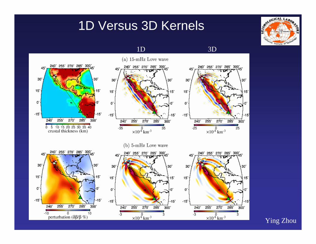
1D Versus 3D Kernels
Ying Zhou
1D 3D

Time-Reversal Imaging: Glacial Earthquakes
Carene Larmat
Greenland

Measuring all available Phase &Amplitude Anomalies


400 800 1200 1600 2000 2400 2800 3200 3600 4000
P PcP pP
sP
PP PKiKP
pPKiKP
sPKiKP
SKiKP
SKSac S
SKKSac
pSKSac pS
sSKSac sS
ScS SPn
PnS SS
SKKSdf
SKKSac
P’P’df
F2=
0.9
3
dT=
1.0
0
F2=
0.8
3
dT=
1.0
0
F2=
0.8
3
dT=
6.0
0
F2=
0.6
8
dT=
2.0
0
F2=
0.7
8
dT=
-1.0
0
400 800 1200 1600 2000 2400 2800 3200 3600 4000
Time (s)
RAR
400 800 1200 1600 2000 2400 2800 3200 3600 4000
Time (s)
F2=
0.91
F2=
0.93
F2=
0.68
F2=
0.92
F2=
0.91
F2=
0.83
F2=
0.84
F2=
0.83
F2=
0.69
F2=
0.85
F2=
0.91
F2=
0.92
F2=
0.51
F2=
0.61
F2=
0.66Seismograms
400 800 1200 1600 2000 2400 2800 3200 3600 4000
Time (s)
Measure all suitable phases
Alessia Maggi
ANMO

ConclusionsAdjoint methods:• Choose an observable, e.g., waveforms or cross-correlation traveltimes• Choose a measure of misfit, e.g., least-squares• Determine the appropriate adjoint source for this observable & measurement• Use fully 3D reference models• Any arrival suitable for measurement• No dependence on the number of stations, components, or measurements• 3D sensitivity kernels may be calculated based upon two forward simulations for each earthquake• Number of simulations: 3 * (# earthquakes) * (# iterations)• Full anisotropy for the same cost• Attenuation remains a challenge
Regional simulations:• One 3 minute forward simulation accurate to 1.5 seconds takes 45 minutes on a 75 node cluster• 150 events and 3 iterations would require 1800 simulations, i.e., three weeks of dedicated CPU time on
75 nodes• Near real-time simulations
Global simulations:• One 1 hour forward simulation accurate to 20 seconds takes 4 hours on a 75 node cluster• 500 events and 3 iterations would require 6,000 simulations, i.e., 100 days on a 750 node cluster• Near real-time simulations• On-demand global seismology• Petascale application
Recommended