South Korean Stock
Exchange and Currency Nabeel Khan, Nemish Kuvadia, Mohit Sibal
I pledge my honor that I have neither received nor provided any unauthorized assistance during
the completion of this work.
12/3/2012
Financial Markets and Instruments
FIN 3560-02
Professor Michael A. Goldstein, PH.D.
Khan, Sibal, Kuvadia
1
Executive Summary
After being left impoverished by the 1948 Korean War, South Korea restructured its political
atmosphere and experienced rapid economic expansion in the decades that followed by becoming an
export driven economy. This has led South Korea to become the fourth largest Asian economy by GDP,
which means today more than ever it is influenced by and exposed to international economies. We wanted
to see the extent to which the Korean stock market and its currency, the Won, is affected by some of its
neighboring East Asian countries, namely China, Japan, Hong Kong and Indonesia. We also wanted to
find out if the relationship was stronger during times of growth or during periods of crisis. Thus, our
paper examines the interdependency of the Korean Stock Exchange and the Won with the economies and
currencies of the above mentioned countries during a growth period, 2002-07, and 2 crisis periods, the
1997-98 East Asian Crisis and the 2008 global financial crisis.
In terms of the stock markets, the results were that the Korean stock market is strongly correlated
with Hong Kong and Indonesia, and only with China and Japan during a crisis. We also found that these
economies more correlated during a period of crisis than a period of economic growth.
In terms of currencies, the data we analyzed showed that the Korean Won is not linked to any of
the currencies of some of its East Asian neighbors, regardless of the economic environment.
The purpose of this paper is to find some trends of the South Korean market and currency with
some of its neighbors in order to forecast how the Korean economy would behave, depending on the
performance of our chosen countries and the economic environment.
Khan, Sibal, Kuvadia
2
Korea Exchange overview
The Korea Exchange (KRX) was created in 2005 through the integration of the Korea Stock
Exchange, Korea Futures Exchange, and the Korean Securities Dealers Automated Quotations
(KOSDAQ).1 However, prior to that the three components of the KRX have been around for much longer.
“The Stock Market division has been operating since 1956 and operated as the sole stock exchange in
Korea until 1996 when the Stock Index Futures Market was launched. Prior to this development,
electronic trading was introduced in 1988. The Stock Index Options Market kicked off operations in 1997
and subsequently, the portfolio of trading instruments was increased at the turn of the century to include
warrant trading, equity options and exchange traded funds (ETFs).” 2
“As of October 2012, Korea
Exchange had 1,796 listed companies with a combined market capitalization of $1.1 trillion.”3
The three main divisions of the KRX are the Korea Composite Stock Price Index (KOSPI)
division, the KOSDAQ division, as well as the derivatives market division. The Korea Exchange provides
an electronic platform for the trading, clearing and settlement of cash equities, bonds and derivatives.4
The Korea Exchange's main stock index is the KRX KOSPI which will also be the main focus of this
paper. “The KOSPI Index is a capitalization-weighted index of all common shares on the Korean Stock
Exchanges. The Index was developed with a base value of 100 as of January 4th, 1980.”5
Going Global
Through the Korea Exchanges recently acquired partnerships with Eurex and the CME Group,
they have expanded their position into the international derivative markets. This allows for distribution
and trading in options and futures on its benchmark KRX KOSPI 200 stock index.6
1 Korea Exchange. http://www.marketswiki.com/mwiki/Korea_Exchange
2 All About the Korea Exchange. http://www.etoro.com/education/all-about-korea-exchange.aspx
3 Korea Exchange. http://en.wikipedia.org/wiki/Korea_Exchange
4 Ibid. 1
5 Bloomberg. Korea Stock Exchange KOSPI Index. http://www.bloomberg.com/quote/KOSPI:IND
6 Ibid. 1
Khan, Sibal, Kuvadia
3
“In November 2009 KRX launched a joint agreement with Chicago-based CME Group to provide
after-hours electronic trading access to KOSPI 200 Futures contracts via the CME Globex platform. KRX
and the CME also agreed on a bi-directional order-routing system similar to that successfully
implemented between the CME and BM&FBOVESPA, Brazil's largest securities-trading exchange.”7
“In August 2010, KRX began listing its KOSPI 200 options contract, also during non-Korean
market hours, on Eurex. The partnership allows Eurex members to trade and clear Kospi 200 options
during European and North American trading hours. The Eurex KOSPI product is a daily futures contract
based on the KOSPI 200 options. These futures contracts expire at the end of each trading day and open
positions are transferred to KRX in the form of a KOPSI option.”8
Largest constitutes of the KRX
The largest firms listed on the KRX in terms of market capitalization include Hyundai Motor,
POSCO, as well as Samsung Electronics. Founded in 1968, POSCO is the third largest company on the
KRX and the world’s fourth largest multinational steel making company. Today POSCO has become
USS-POSCO forming some partnerships with some US companies and has a cap of $32.6 billion.9
Subsequently, Hyundai Motor is the largest automaker in Korea and the second largest firm on
the KRX. Established in 1967, it is now the fifth largest car manufacturer in the world by expanding its
presence into many overseas economies such as China, the USA, and India etc. It has a market cap of
$49.8 billion.10
Lastly, more than three times bigger than the second largest firm listed on the KRX in terms of
market cap, Samsung Electronics has a market cap of $165.2 billion. Founded in 1969, the conglomerate
7 Ibid. 1
8 Ibid. 1
9 South Korea’s 10 biggest companies. http://www.cnbc.com/id/48237596/page/9
10 South Korea’s 10 biggest companies. http://www.cnbc.com/id/48237596/page/10
Khan, Sibal, Kuvadia
4
is now the world’s largest producer of smartphones, memory chips, and televisions. Accounting for one-
fifth of the Korean GDP, the Samsung group has a significant impact on Korea’s economy.11
Gaining Competitive Advantage
Korea Exchange is responding to global changes in the stock exchange industry and securing
market competitiveness by implementing the Vertical Silo model in order to run the stocks and
derivatives market.12
“This means that KRX is equipped with stable and efficient stock trading
infrastructure that provides one-stop services for core capital markets functions, such as trading, order
execution, clearing, and settlement.”13
In order to build a Vertical Silo model, many exchanges worldwide
such as the NYSE Euronext, Nasdaq OMX, and LSE etc. are taking over clearing houses such as
LCH.Clearnet. The KRX has a much better advantage as its derivatives market has abundant liquidity.
Along with that, due to Korea’s remarkable information technologies, KRX has pushed forward into
overseas markets, in particular South Asian markets, as there is a tremendous prospective for growth.14
For example: “In Laos, KRX took over the Lao Securities Exchange’s stakes and jointly opened a stock
exchange; it exported Korea’s IT trading infrastructure for bond trading, supervision, and market making
monitoring to Bursa Malaysia. Furthermore, KRX has plans to export its stock trading system, market
monitoring system, and expertise to Cambodia, Vietnam, and Philippines.”15
Along with that, the KRX
plans to move into central Asia, where the infrastructure for stock trading is not as developed, starting
with Uzbekistan.
In addition, the KRX has been developing a new generation IT system called the New Exture
which will increase stock trading stability, allow for progressive transaction services such as high
frequency trading, and allow for KRX to secure a strong position in the global markets for stock trading
11
South Korea’s 10 biggest companies. http://www.cnbc.com/id/48237596/page/11 12
Competition in the Global Capital Markets and Challenges Ahead for the KRX 13
Ibid. at Page 3 14
Ibid. at Page 3 15
Ibid. at Page 4
Khan, Sibal, Kuvadia
5
IT systems.16
“KRX rivals include NYSE Euronext, which exported its stock trading system to Malaysia
and Philippines, and Nasdaq OMX, which exported its stock trading system to Singapore and Indonesia
and sold its derivatives system to Thailand.”17
However, the New Exture system will allow the KRX to
provide more advantages than other competitors. Pushing KRX’s stocking trading model overseas will
help increase awareness as well as competitiveness, permitting for an increase in revenue.
Regulation
The Korean stock market is regulated by the Korea Exchange. The Financial Supervisory
Services (FSS) has given the KRX the self-regulatory authority. The main roles of the KRX involve
“maintaining a fair and orderly organized market, regulating and supervising the member firms, setting
listing requirements, surveillance of securities transactions and regulating corporate disclosure”18
. In order
for companies to receive acceptance on listing they must submit the listing application to KRX, which
must then be approved by the Financial Supervisory Service (FSS).19
The KRX is primarily responsible
for settling all transaction on the stock exchange and is liable for all the damages. The secondary bond
market has been divided into three segments, namely the KRX, an organized exchange and the OTC
market20
. The KRX market for bonds is a competitive trading of listed bonds, whereas the OTC market is
the most dominant form of bind trading in South Korea21
. With the introduction of several derivatives
products, there were increased supervision and compliance procedures for financial institutions under the
amended Financial Investment Services and Capital Markets Act22
. The KRX introduced a system of
“Circuit Breaker” for the KOSPI 200 Futures financial product when the derivative hits ±5% of previous
16
Ibid. at Page 4 17
Ibid. at Page 4 18
Financial Supervisory System in Korea. Page 24. Retrieved from
http://www.fsc.go.kr/downManager?bbsid=BBS0049&no=61122 19
Ibid. at Page 109 20
Ibid. at Page 111 21
Ibid. at Page 111 22
Ibid. at Page 111
Khan, Sibal, Kuvadia
6
closing.23
The use of circuit breakers would allow market participants to accumulate more information so
as to make informed choices during the period when trading is halted on a particular derivatives product.
Comparison between Futures Trading Act and Financial Investment Services and Capital Markets
Act
The Futures Trading Act was enacted in 1995 in South Korea in order to make sure that the
Futures derivatives were traded in a safe manner for the protection of investors. 24
The Act talks about the
manner in which a futures product can only be traded on the futures exchange and only a corporation with
certain equity capital be allowed to trade in futures. 25
The Act mentions the fines and punishment that will
be imposed for indulging in unfair practices on the futures trading market.26
But the Act fails to talk about
the manner in which futures trading corporations can eliminate futures trading manipulation.
The Financial Investment Services and Capital Markets Act passed in 2009 talks about the
manner in which financial investment firms would require to have a full time auditor as well as an audit
committee that would look into the financial statements of the firm.27
The Act also mentions that financial
firms require to appoint a “Compliance Officer”, who would look into the internal controls and
procedures followed by the firm and report his or her findings to the audit committee.28
23
Ibid. at Page 112 24
Financial Supervisory System in Korea. Page 113. Retrieved from
http://www.fsc.go.kr/downManager?bbsid=BBS0049&no=61122 25
Futures Trading Act. Page 1 Retrieved from
http://unpan1.un.org/intradoc/groups/public/documents/apcity/unpan011495.pdf 26
Ibid. 27
Ibid. 28
Korea Financial Investment Association (KOFIA). Financial Investment Services and Capital Markets Act.
Rerieved from
http://www.kofiabond.or.kr/ENG/DATA/Financial%20Investment%20Services%20and%20Capital%20Markets%2
0Act.pdf
Khan, Sibal, Kuvadia
7
New Amendments in the Korean Stock Exchanges
There have been a few amendments in the past year that have brought about a change in the way
trading is executed on the Korean Stock Exchanges. The first area in which there is a new rule is the area
of short selling. The FSS, FSC and the KRX have come to a conclusion that all individual investors who
have a position on short selling in the market have to report their positions to the regulator at the end of
each trading day.29
The threshold set by the regulators of the short selling position on investors is set at
“0.01% of the issued share capital of a listed company”.30
This move is particularly helpful during
uncertain domestic as well international economics conditions and keeps a check on fair trading during
these volatile economic times.
Statistical Analysis of KOSPI vs. East Asian Neighbors
As we wanted to see how correlated the Korean markets are to China, Japan, Hong Kong and
Indonesia, we ran regressions of the Korean KOSPI against the major benchmark indexes of the other
countries. Due to the fact that we also wanted to see if the East Asian markets are more correlated during
growth periods or crisis periods, we used data from the East Asian Crisis during 1997-98, the global
financial crisis during 2008-12, and the growth period that occurs in-between, from 2002-07.
In terms of the crisis periods, we chose the two most recent crises that have affected Asian
markets. The first was the East Asian Crisis that began due to the outflow of money from East Asia to
other parts of the world with higher interest rates.31
“Thailand was the first to have to float the Thai Bhat,
this caused a rapid devaluation, which triggered a loss of confidence throughout the Asian economies.”32
29
FSC, FSS, and KRX plan introduction of short position reporting rules. Retrieved from http://www.theasianbanker.com/updates?&docid=0008109725031185%20312081208 30
Ibid. 31 The 1997-1997 Asian Financial Crisis http://www.economicshelp.org/dictionary/f/financial-crisis-asia-1997.html
32 Ibid.
Khan, Sibal, Kuvadia
8
This began a ripple effect, where economies of other Asian countries also began decreasing. The
South Korean economy in particular dropped 30 percent at the peak of the crisis, and was eventually
given $57 billion USD by the IMF in order to stabilize its currency and economy.33
The second was the
2008 global financial crisis that began in the United States. The depression had worldwide repercussions,
affecting most of the world’s economies and had aftereffects until the present day as many economies are
still struggling to recover.
The reason we chose the five year time period from 2002-2007 was because the economies of the
world collectively saw positive GDP growth.34
World output grew 3.22% per year, and in particular, East
Asian economies during the time period averaged 7.48% GDP growth per year.35
Our data is based on monthly data. Regressions with a p-value of less than 0.05 are considered
significant.
Growth; 2002-2007
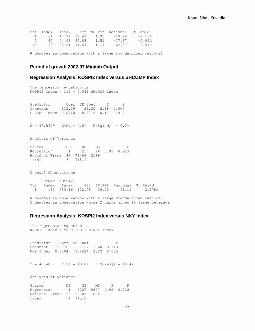
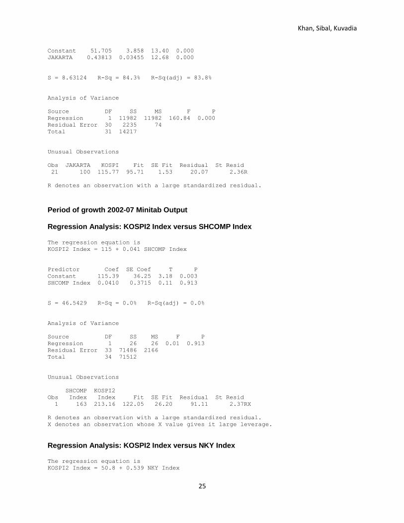
Comparing the KOSPI with the SHCOMP (Shanghai Composite Index), we got an R2 value of
0.0%, which indicates there is absolutely no correlation of the Korean markets with the Chinese markets
during this growth period. This is mitigated by the fact that the p value is 0.913, which indicates the
regression is not statistically significant. Thus, it cannot be said that the SCHOMP is completely un-
correlated with the KOSPI during this period.
Comparing the KOSPI with the NIKKEI, we got an R2 value of 13.0%, with a p value of 0.033
indicating the test is statistically significant. This data shows that the Korean markets and the Japanese
markets are not very correlated.
33
Ibid. 34 World Economic Situation and Prospects 2007
http://www.un.org/en/development/desa/policy/wesp/wesp_archive/2007wespupdate.pdf; source;
http://www.un.org/en/development/desa/index.html
35
Ibid.
Khan, Sibal, Kuvadia
9
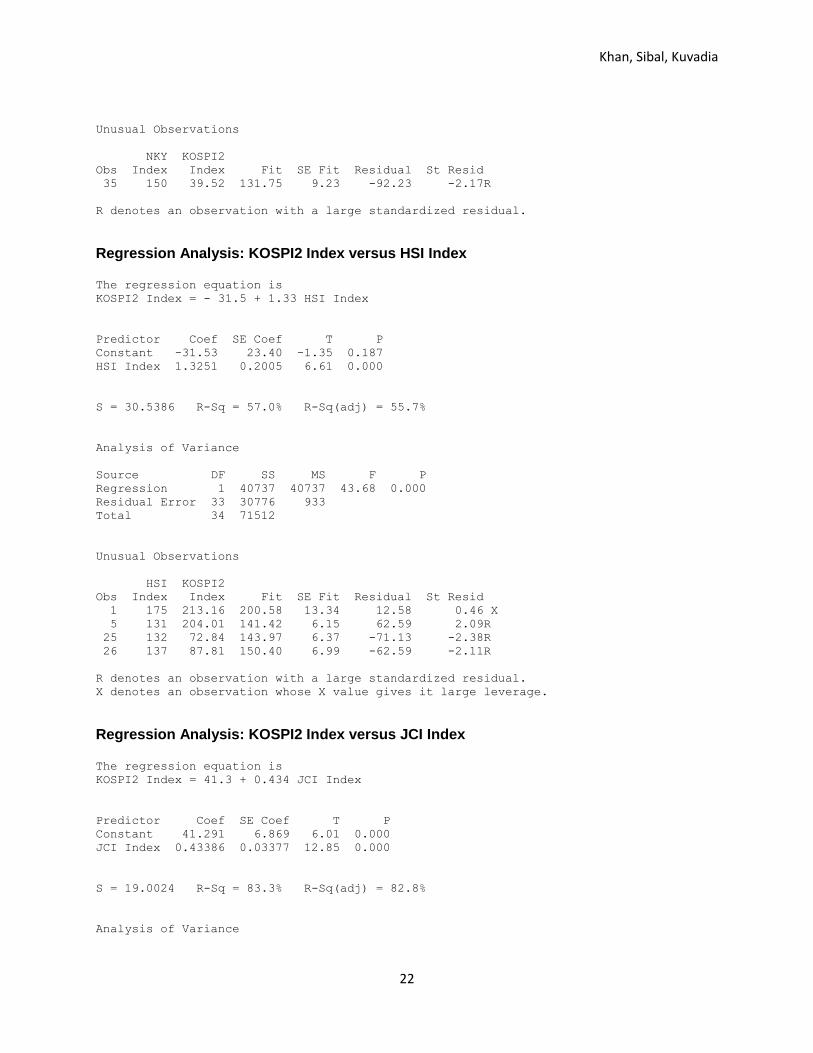
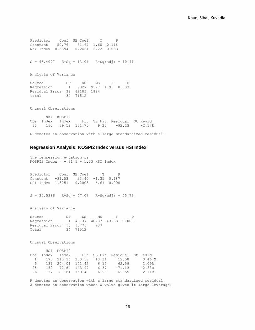
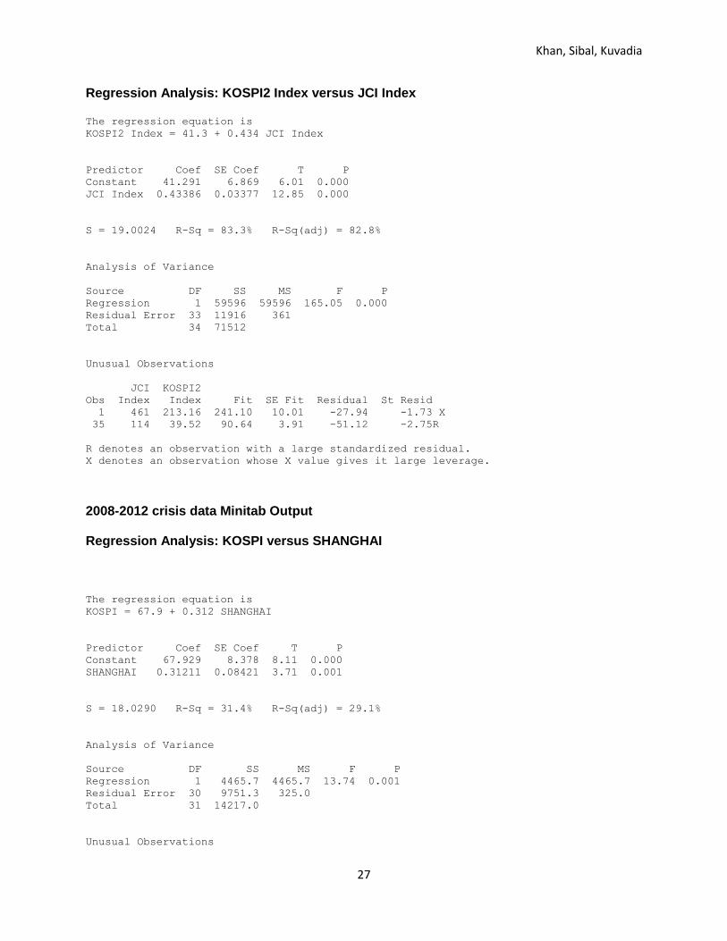
Unlike the other two markets, the regressions we ran with the KOSPI against the Hang Seng
Composite Index and the JCI (Jakarta Composite Index) showed that the Hong Kong market and the
Indonesian markets were quite strongly correlated with the Korean market. Against the Hang Seng, we
got an R2 value of 57%, and against the JCI, an R
2 value of 83.3%. Both the p values were under 0.05,
showing the regression was statistically significant.
Thus, during the growth period of 2002-2007, the regressions we ran showed us that the Korean
stock exchange was quite strongly correlated with the Hong Kong exchange and the Jakarta exchange,
and not so much with the Chinese and the Japanese stock markets.
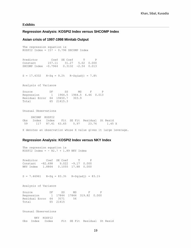
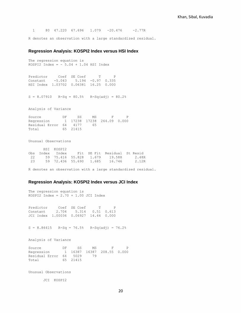
Crisis 1; 1997-1998
Comparing the KOSPI with the SHCOMP we got an R2 value of 9.2%. The p value we got was
0.013, indicating the regression was statistically significant. This low R2 value suggests almost no
correlation between the two markets, and goes against our hypothesis that the Korean and Chinese stock
markets would be linked.
This was an exception though, as the KOSPI was extremely correlated to the other stock
exchanges; there was a 83.3% correlation with the NIKKEI, 80.5% with the Hang Seng, and 76.5% with
the JCI. All of the p values were below 0.05, which indicates all of these regressions were statistically
significant. This data shows that during the East Asian Crisis, the Korean markets are linked with most of
the countries we chose.
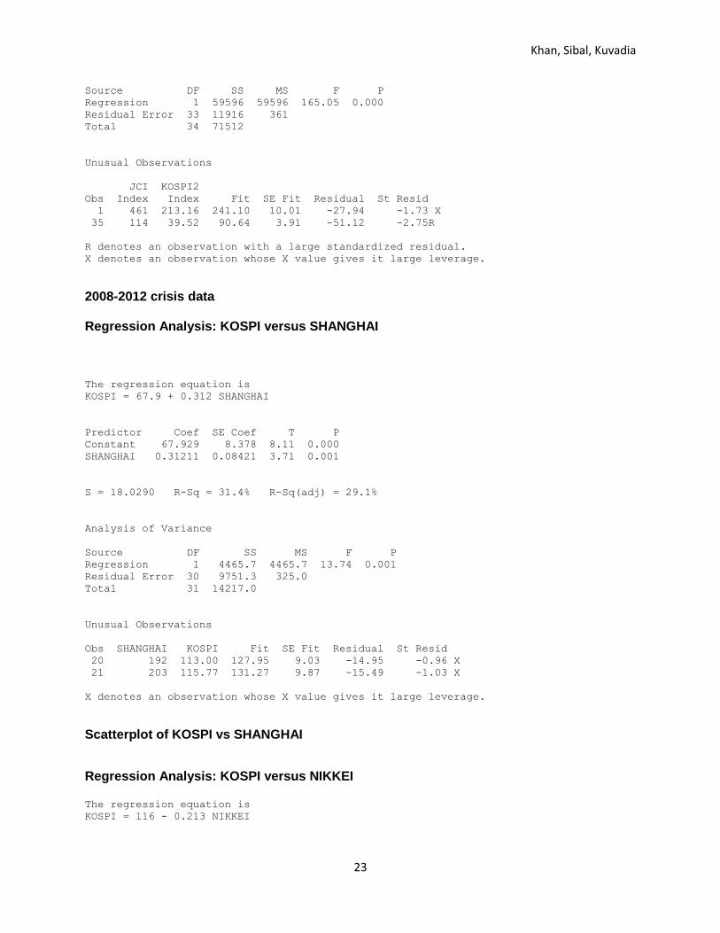
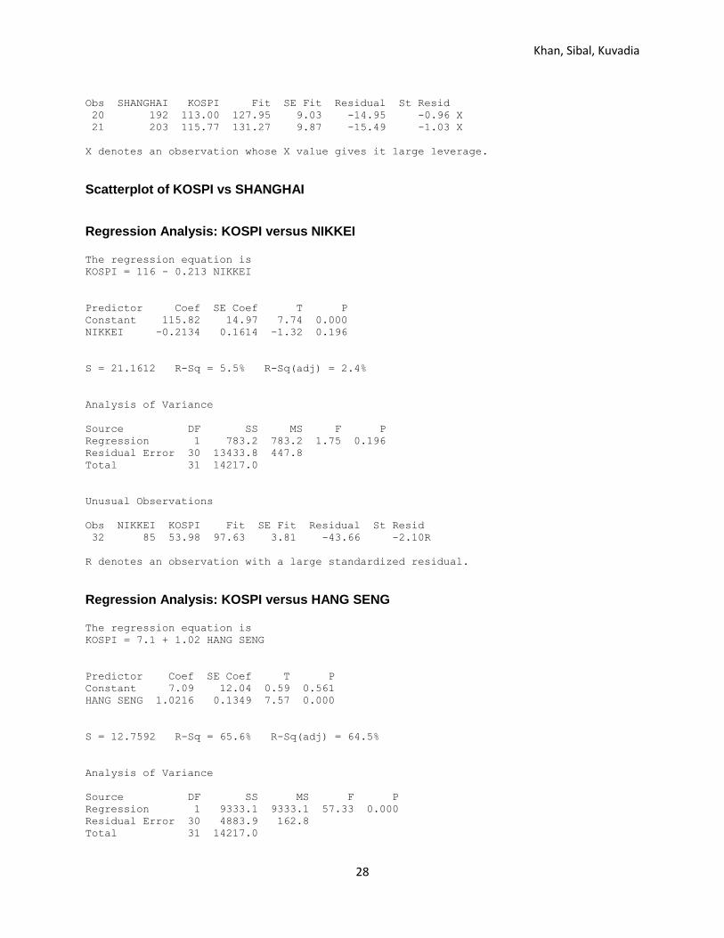
Crisis 2; 2008-2012
Comparing the KOSPI with the SHCOMP, we got an R2 value of 31.4%, with a p value of 0.001
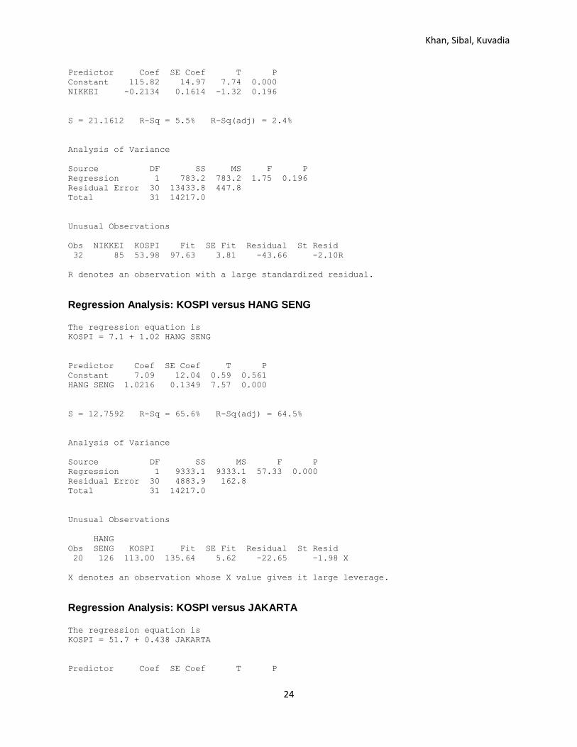
showing statistical significance. Against the NIKKEI, we got an R2 value of 5.5%, showing that during
this crisis period, the Japanese markets were not correlated with the Korean markets. Although this goes
against our hypothesis, the p value for this test was 0.196, which means it was not statistically significant.
Khan, Sibal, Kuvadia
10
The Hang Seng and the JCI were strongly correlated during the global financial crisis. This is
shown with the R2 values we got regressing against the KOSPI, which were 65.6% and 84.3%
respectively. The p values under 0.05 show the regression was statistically significant.
Thus, during the global financial crisis period of 2008-2012, the regression data shows the
Korean stock exchange was strongly correlated with Hong Kong and Jakarta, and fairly correlated with
Shanghai. We had to dismiss the regression against Japan because it was not statistically significant.
Statistical Analysis of Korean Won Vs. East Asian Neighbors
The data that we compiled for each time period was monthly. Regressions with a p-value of less
than 0.05 are considered significant. The x-values in our regression represent the Korean Won and the y-
values include the currencies of China, Japan, Hong Kong and Jakarta.
Growth; 2002-2007
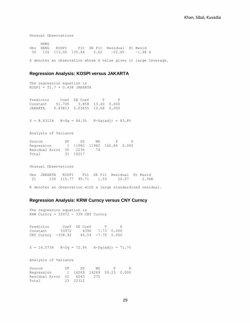
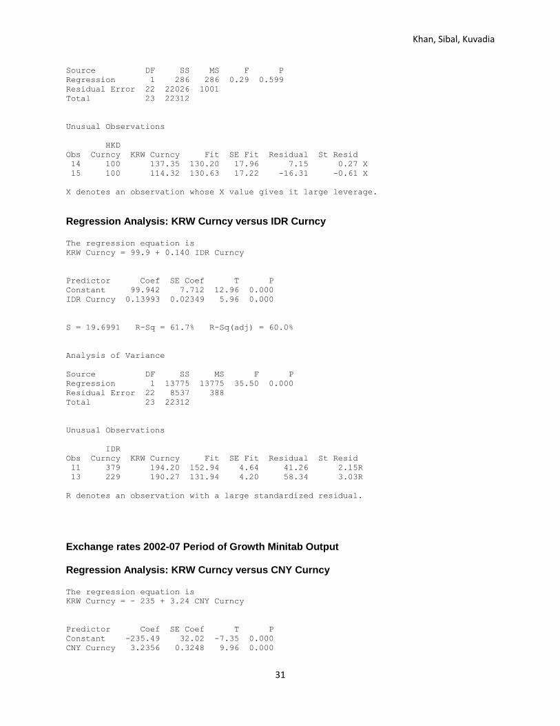
First, we ran a regression between the Korean Won and the Chinese Yuan during the growth
period. The linear regression equation is y = - 235 + 3.24x and its p-value is 0.000, thereby indicating that
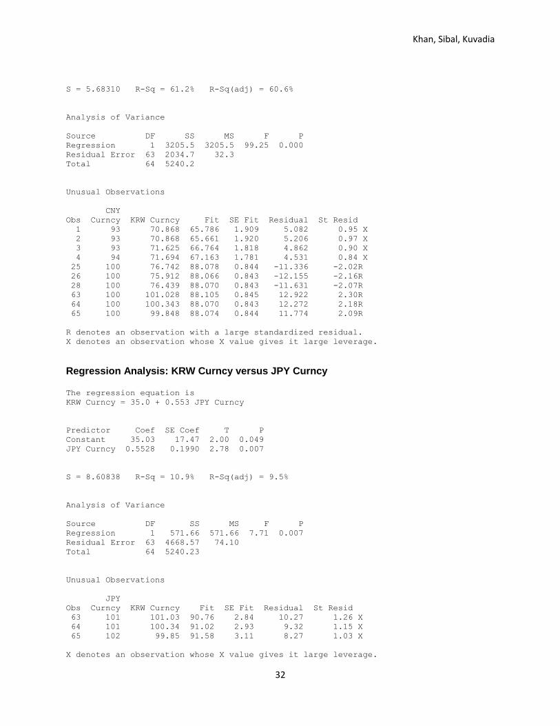
the regression is statistically significant. The R-sq of the above equation is 61.2%, which shows that a
61% of the variation in the Yuan can be explained by the variation in the Korean Won. This is particularly
a high number looking at the number of data points that we had while running the regression. Thus the
Chinese Yuan shows a strong correlation with the Korean Won during this time period.
Then we ran a regression between the Korean Won and the Japanese Yen and the equation that
we get is y = 35.0 + 0.553x and the p-value is 0.007, which shows that the regression is statistically
significant. The R-sq of the equation is 10.9%, which indicates that the currencies are not strongly
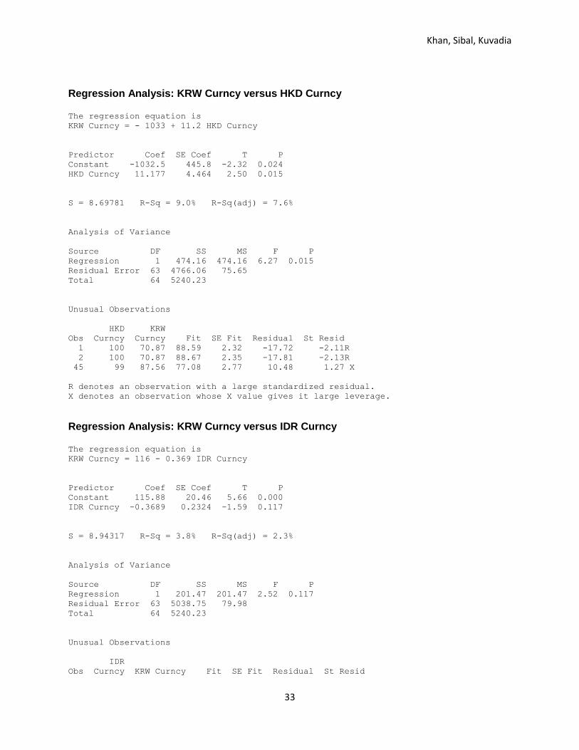
correlated during the growth period. Next, we ran a regression between the Won and the Hong Kong
dollar. The equation of the regression is y = - 1033 + 11.2x and the p-value was 0.015, which shows that
the regression was statistically significant. The positive x-variable shows a positive relation between the
Khan, Sibal, Kuvadia
11
currencies but the R-sq of the regression is 9%, which shows that the currencies do not have strong
correlation during the time period.
The last regression we ran during the growth period was between the Won and the Indonesian
Rupiah. The linear regression we get is y= 116 - 0.369x and a p-value of 0.117, which shows that the
regression was not statistically significant. The R-sq we get is 3.8%, which is extremely low and shows
that the currencies are not strongly correlated. Thus by running all the regressions during the period of
growth, we see a general trend that the currencies are not strongly correlated with the exception of the
Chinese Yuan.
Crisis 1; 1997-1998
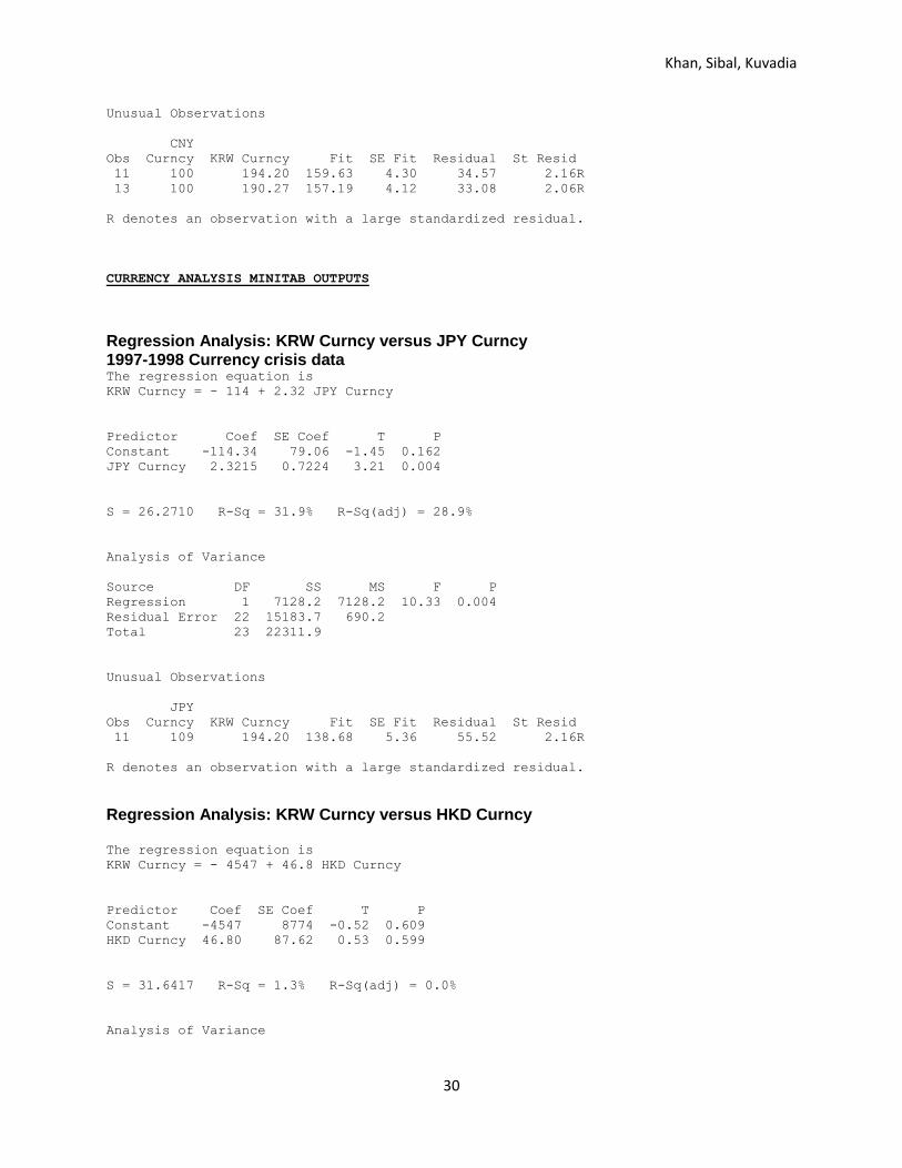
During the Asian crisis of 1997 and 1998, we ran a simple regression between the Korean Won
and the above mentioned currencies. The regression equation for the relation with the Yuan is y= 33972 –
339x with a p-value of 0.00, which shows that regression is statistically significant. The R-sq is 72.9%,
which is very high, shows a strong correlation between the currencies. The regression equation with the
Japanese Yen is y= - 114 + 2.32x, with a p-value of 0.004, which shows the regression is statistically
significant. The R-sq is 31.9%, which is low and confirms our hypothesis of a weak correlation between
the currencies.
The regression equation with the Hong Kong dollar is regression equation is y = - 4547 + 46.8x
with a p-value of 0.599, which shows that the regression is not statistically significant. The R-sq is 1.3%,
which confirms our hypothesis of a low correlation between the currencies. The regression equation with
the Indonesian Rupiah is y = 99.9 + 0.140x with a p-value of 0.00 that shows that the regression is
statistically significant. The R-sq is 61.7%, which is particularly high, which shows a strong correlation
between the currencies during that time period.
Khan, Sibal, Kuvadia
12
Crisis 2; 2008-2012
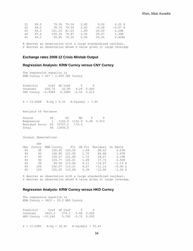
During the global financial crisis, the regression equation that we get for the Chinese Yuan is y =
116 - 0.369x and a p-value of 0.013, which shows the regression is statistically significant. The R-sq of
9.3% and the negative x-variable coefficient shows a weak correlation between the currencies. When we
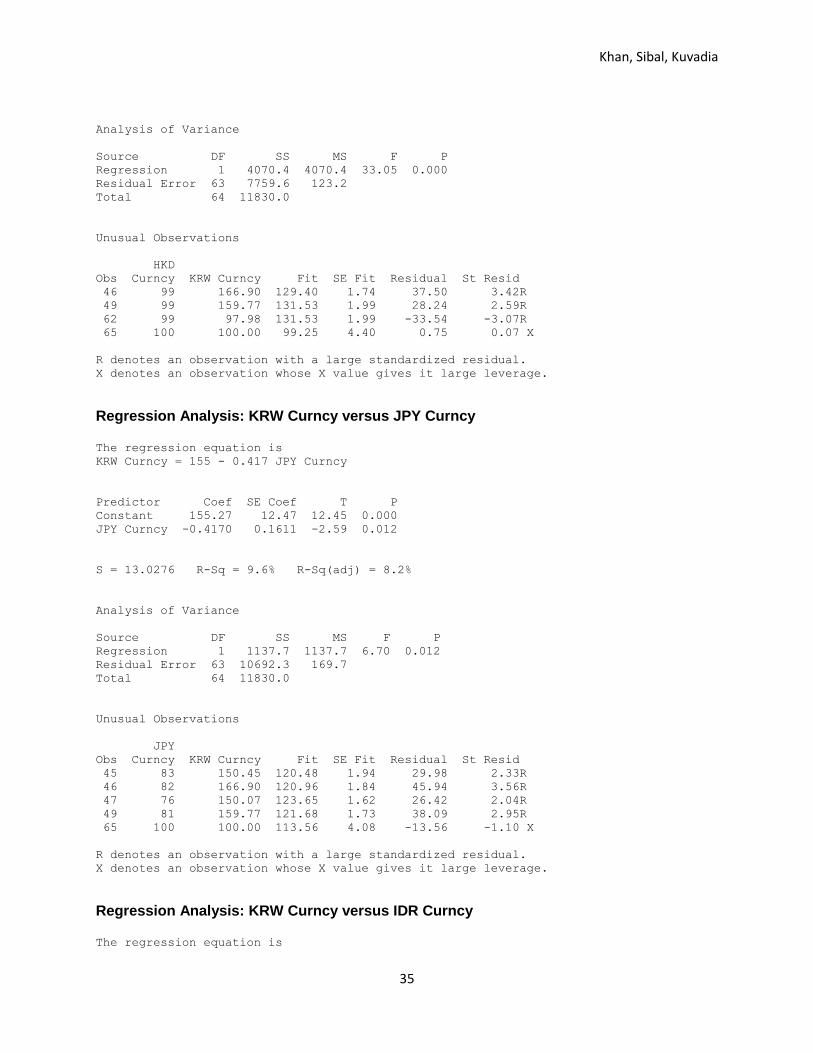
compared the Korean Won to the Japanese Yen, the regression equation we get is y = 155 - 0.417x, with a
p-value of 0.012, which indicates statistical significance. The R-sq of 9.6% suggests not a very strong
correlation between the two currencies during the crisis.
The Hong Kong dollar’s regression equation is y = 3423 - 33.2x and a p-value of 0.000 shows
that the regression is statistically significant. The R-sq is 34.4%, which is relatively low, showing little
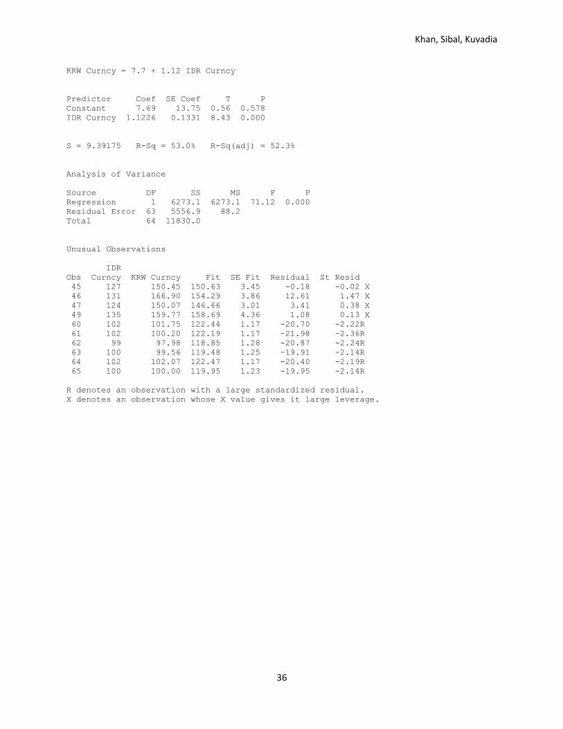
correlation in the two country’s currencies. When we compared the Indonesian Rupiah to the Won, the
regression equation we get is y = 7.7 + 1.12x with a p-value of 0.00 indicating statistical significance. The
R-sq of 53% shows that there was a relatively strong correlation between the two currencies in
comparison to the others. Thus, during the second crisis period, the general trend again shows the
currencies are not strongly correlated, with the exception of the Rupiah.
Reasons for Correlation
From the time period of 2002 till 2007, we see a high correlation between the Chinese Yuan and
the Korean Won. A possible explanation for that could be the fact that the Chinese Yuan had stabilized at
the 8.28 RMB/USD rate for about 10 years till 2005. 36
After that though, the Chinese Yuan started
depreciating rapidly till the end of our model at, the end of 2006. The Korean Won’s depreciation had
since the beginning of the model (1st Jan 2002) combined with the Yuan’s rapid depreciation from 2005-
2007 explains the correlation between the currencies.
36
The Case for Stabilizing China’sExchange Rate: Setting the Stage for Fiscal Expansion. Retrieved from http://www.stanford.edu/~mckinnon/papers/fulltext_McKinnon%20and%20Schnabl.pdf Page 5
Khan, Sibal, Kuvadia
13
The Japanese central bank intervened between 2003 and 2004 on several occasions in order to
weaken the Yen.37
Thus the Yen depreciated and appreciated at several occasions between the time
periods of our model, whereas the Korean Won consistently depreciated during the time period. This
explains the weak correlation in the Japanese and Korean currencies as Japan intervened several times
bringing down the value of its currency and appreciating briefly again.
The Hong Kong dollar has been firmly pegged to the US dollar since 1983, thus the Hong Kong
dollar was trading in a very narrow trading range due to its hard peg to the US dollar.38
The Korean
Won’s constant depreciation during the regression model’s time period and the wide range that the
currency was trading combined by the narrow range the Hong Kong dollar was trading was the reason for
the low correlation of their currencies.
During the financial crisis of 2008, the South Korean central bank and the Indonesian central
bank intervened in the foreign exchange markets in order to buy dollars to keep a check on their country’s
currency appreciation.39
This was particularly done by the country’s central banks in order to keep their
competitive advantage in the international exports markets.The similar proportions of USD buying during
the central bank interventions may be the reason for the relatively strong correlations in comparison to
other currencies.
Japan also intervened during the financial crisis at multiple occasions but the proportions in
comparison to the rest of the countries were much higher. Between September 2010 and October 2011,
the Japanese central bank intervened by buying as much as $100 billion USD.40
The Japanese central
bank did this in order to weaken the value of the Yen in order to remain competitive in the international
37
An Assessment of the Impact of Japanese Foreign Exchange Intervention: 1991-2004 . Retrieved from http://www.federalreserve.gov/pubs/ifdp/2005/824/ifdp824.pdf . Page 11 38
Hong Kong faces heat on dollar peg. Retrieved from http://www.ft.com/intl/cms/s/0/6a6988b6-e774-11df-b5b4-00144feab49a.html#axzz2Dq9YuxCB 39
Asian Central Banks Intervene as Currencies Rise. Retrieved from http://online.wsj.com/article/SB10001424052748704503104576250402542030250.html 40
Does Foreign Exchange Intervention Volume Matter?. Retrieved from http://www.dallasfed.org/assets/documents/institute/wpapers/2012/0115.pdf Page 2
Khan, Sibal, Kuvadia
14
exports market, being an export driven nation themselves. This number is extraordinary high in
comparison to the interventions of Korea, Indonesia and Hong Kong. Thus we can conclude that during
the financial crisis, the Yen appreciated at multiple occasions and the central bank intervened in the FX
market buying USD’s in a much higher proportion as opposed to the Korean central bank. This could be a
cause for the weak correlation between their currencies.
Khan, Sibal, Kuvadia
15
Conclusion
Our data showed us that during a period of growth, the markets of only Hong Kong and Jakarta
moved with Korea, but during a period of crisis, Japan and China also joined that list. This shows that
during a crisis period, the East Asian economies are more linked with one another. We speculate that a
reason for this is market sentiment is stronger during a crisis period; the fear of losing money is a stronger
driver of decision making than the speculation of making money.
While the stock markets show some signs of interdependency, this is not the case with currencies.
We say this because we did not find a general trend when analyzing the data. For example, one country’s
currency correlation might have happened during one crisis, but the same correlation did not occur during
the other crisis. We found reasons that shed light to why this was happening, which ultimately led us to
the conclusion that there is no definitive correlation between the currencies of the East Asian countries we
chose, regardless of economic environment.
The reason we performed these regressions was in order to find some trends with some of South
Korea’s East Asian neighbors in order to make a forecast how the Korean stock market would behave.
Through our analysis, we can say that the Korean market is strongly correlated with the markets of Hong
Kong and Indonesia, regardless of economic environment. Thus, our recommendation to foreign investors
looking to add South Korea to their investment portfolio would be to look at how the stock markets of
Hong Kong and Indonesia are performing and invest accordingly.
Khan, Sibal, Kuvadia
16
References
"All about the Korea Exchange." EToro. Cyprus Securities Exchange Commission,
n.d. Web. 29 Nov. 2012. http://www.etoro.com/education/all-about-korea-exchange.aspx
Bloomberg LP (2012). Korean stock Index v/s Shanghai Composite Index, Nikkei Index, Hang Seng
Composite Index, Jakarta Composite Index from January 1997-december 1998, January 2002-
December 2006, January 2007-29th November 2012.
Bloomberg LP (2012). Korean Won v/s Chinese Yuan, Japanese Yen, Hong Kong dollar, Indonesian
Rupiah from January 1997-December 1998, January 2002-December 2006, January 2007- 29th
November 2012
Bloomberg LP (2012). Korean Won v/s Yuan, Yen, Hong Kong dollar, Indonesian Rupiah. Price chart
comparison. Steps: G<Go> CreateChart Put in currenciesFinish
Chaboud, Alain & Humpage, Owen. “An Assessment of the Impact of Japanese Foreign Exchange
Intervention: 1991-2004”. International Finance Discussion Papers Number 824 January 2005.
Retrieved from http://www.federalreserve.gov/pubs/ifdp/2005/824/ifdp824.pdf
Department of Economic and Social Affairs. Retrieved from
http://www.un.org/en/development/desa/index.html
Director, Martin. “THE ECONOMIC CRISIS IN EAST ASIA: CAUSES, EFFECTS, LESSONS”. Third
World Network. Retrieved from http://www.ifg.org/khor.html
Fatum, Rasmus & Yamamoto, Yohei. “Does Foreign Exchange Intervention Volume Matter?”. Federal
Reserve Bank of Dallas Globalization and Monetary Policy Institute Working Paper No. 115.
Retrieved from http://www.dallasfed.org/assets/documents/institute/wpapers/2012/0115.pdf
Khan, Sibal, Kuvadia
17
Financial Crisis Asia 1997. Retrieved from http://www.economicshelp.org/dictionary/f/financial-crisis-
asia-1997.html
Financial Supervisory System in Korea. Retrieved from
http://www.fsc.go.kr/downManager?bbsid=BBS0049&no=61122
“Financial Investment Services and Capital markets Act”. Korea Financial Investment Association.
Retrieved from
http://www.kofiabond.or.kr/ENG/DATA/Financial%20Investment%20Services%20and%20Capit
a l%20Markets%20Act.pdf
“FSC, FSS, and KRX plan introduction of short position reporting rules”. The Asian Banker. Retrieved
from http://www.theasianbanker.com/updates?&docid=0008109725031185%20312081208
Futures Trading Act. United Nations. Ministry of Legislation. Retrieved from
http://unpan1.un.org/intradoc/groups/public/documents/apcity/unpan011495.pdf
Kim, Bung. “Competition in the Global Capital Markets and Challenges Ahead for the KRX.”.
"Korea Exchange." MarketsWiki. N.p., n.d. Web. 12 Nov. 2012.
http://www.marketswiki.com/mwiki/Korea_Exchange
"Korea Stock Exchange KOSPI Index." Bloomberg. Bloodberg, n.d. Web. 1 Dec. 2012.
http://www.bloomberg.com/quote/KOSPI:IND
McKinnon, Ronald & Schnabl, Gunther. “The Case for Stabilizing China’s Exchange Rate: Setting the
Stage for Fiscal Expansion”. China & World Economy / 1 – 32, Vol. 17, No. 1, 2009. Retrieved from
http://www.stanford.edu/~mckinnon/papers/fulltext_McKinnon%20and%20Schnabl.pdf
Khan, Sibal, Kuvadia
18
Nanto, Dick. “THE 1997-98 ASIAN FINANCIAL CRISIS”. CRS Report for Congress. Retrieved from
http://www.fas.org/man/crs/crs-asia2.htm
Sender, Henny. “Hong Kong faces heat on dollar peg”. Retrieved from
http://www.ft.com/intl/cms/s/0/6a6988b6-e774-11df-b5b4-00144feab49a.html#axzz2Dq9YuxCB
"South Korea's 10 Biggest Companies." CNBC.com. Thomson Reuters, n.d. Web. 27
Nov. 2012. http://www.cnbc.com/id/48237596
Venkat, P. “Asian Central Banks Intervene as Currencies Rise”. Retrieved from
http://online.wsj.com/article/SB10001424052748704503104576250402542030250.html
What Caused East Asia's Financial Crisis?. FRBSF Economic Letter. Retrieved from
http://www.frbsf.org/econrsrch/wklyltr/wklyltr98/el98-24.html
World Economic Situationand Prospects 2007. Retrieved from
http://www.un.org/en/development/desa/policy/wesp/wesp_archive/2007wespupdate.pdf.
Page 2 Table Source: Department of Economic and Social Affairs of the United Nations
Secretariat.
“The authors of this paper hereby give permission to Professor Michael Goldstein to distribute this paper
by hard copy, to put it on reserve at Horn Library at Babson College, or to post a PDF version of this
paper on the internet”.
Khan, Sibal, Kuvadia
19
Exhibits
Regression Analysis: KOSPI2 Index versus SHCOMP Index Asian crisis of 1997-1998 Minitab Output The regression equation is
KOSPI2 Index = 157 - 0.796 SHCOMP Index
Predictor Coef SE Coef T P
Constant 157.11 31.27 5.02 0.000
SHCOMP Index -0.7964 0.3132 -2.54 0.013
S = 17.4332 R-Sq = 9.2% R-Sq(adj) = 7.8%
Analysis of Variance
Source DF SS MS F P
Regression 1 1964.5 1964.5 6.46 0.013
Residual Error 64 19450.7 303.9
Total 65 21415.3
Unusual Observations
SHCOMP KOSPI2
Obs Index Index Fit SE Fit Residual St Resid
59 117 87.41 63.65 5.97 23.76 1.45 X
X denotes an observation whose X value gives it large leverage.
Regression Analysis: KOSPI2 Index versus NKY Index The regression equation is
KOSPI2 Index = - 82.7 + 1.89 NKY Index
Predictor Coef SE Coef T P
Constant -82.698 9.022 -9.17 0.000
NKY Index 1.8864 0.1055 17.88 0.000
S = 7.46961 R-Sq = 83.3% R-Sq(adj) = 83.1%
Analysis of Variance
Source DF SS MS F P
Regression 1 17844 17844 319.82 0.000
Residual Error 64 3571 56
Total 65 21415
Unusual Observations
NKY KOSPI2
Obs Index Index Fit SE Fit Residual St Resid
Khan, Sibal, Kuvadia
20
1 80 47.220 67.696 1.079 -20.476 -2.77R
R denotes an observation with a large standardized residual.
Regression Analysis: KOSPI2 Index versus HSI Index The regression equation is
KOSPI2 Index = - 5.04 + 1.04 HSI Index
Predictor Coef SE Coef T P
Constant -5.043 5.194 -0.97 0.335
HSI Index 1.03702 0.06381 16.25 0.000
S = 8.07910 R-Sq = 80.5% R-Sq(adj) = 80.2%
Analysis of Variance
Source DF SS MS F P
Regression 1 17238 17238 264.09 0.000
Residual Error 64 4177 65
Total 65 21415
Unusual Observations
HSI KOSPI2
Obs Index Index Fit SE Fit Residual St Resid
22 59 75.416 55.828 1.679 19.588 2.48R
23 59 72.436 55.690 1.685 16.746 2.12R
R denotes an observation with a large standardized residual.
Regression Analysis: KOSPI2 Index versus JCI Index The regression equation is
KOSPI2 Index = 2.70 + 1.00 JCI Index
Predictor Coef SE Coef T P
Constant 2.704 5.314 0.51 0.613
JCI Index 1.00036 0.06927 14.44 0.000
S = 8.86415 R-Sq = 76.5% R-Sq(adj) = 76.2%
Analysis of Variance
Source DF SS MS F P
Regression 1 16387 16387 208.55 0.000
Residual Error 64 5029 79
Total 65 21415
Unusual Observations
JCI KOSPI2
Khan, Sibal, Kuvadia
21
Obs Index Index Fit SE Fit Residual St Resid
1 64 47.22 66.42 1.35 -19.20 -2.19R
2 60 44.96 62.83 1.51 -17.87 -2.05R
43 69 93.91 71.64 1.17 22.27 2.54R
R denotes an observation with a large standardized residual.
Period of growth 2002-07 Minitab Output Regression Analysis: KOSPI2 Index versus SHCOMP Index The regression equation is
KOSPI2 Index = 115 + 0.041 SHCOMP Index
Predictor Coef SE Coef T P
Constant 115.39 36.25 3.18 0.003
SHCOMP Index 0.0410 0.3715 0.11 0.913
S = 46.5429 R-Sq = 0.0% R-Sq(adj) = 0.0%
Analysis of Variance
Source DF SS MS F P
Regression 1 26 26 0.01 0.913
Residual Error 33 71486 2166
Total 34 71512
Unusual Observations
SHCOMP KOSPI2
Obs Index Index Fit SE Fit Residual St Resid
1 163 213.16 122.05 26.20 91.11 2.37RX
R denotes an observation with a large standardized residual.
X denotes an observation whose X value gives it large leverage.
Regression Analysis: KOSPI2 Index versus NKY Index The regression equation is
KOSPI2 Index = 50.8 + 0.539 NKY Index
Predictor Coef SE Coef T P
Constant 50.76 31.67 1.60 0.118
NKY Index 0.5394 0.2424 2.22 0.033
S = 43.4097 R-Sq = 13.0% R-Sq(adj) = 10.4%
Analysis of Variance
Source DF SS MS F P
Regression 1 9327 9327 4.95 0.033
Residual Error 33 62185 1884
Total 34 71512
Khan, Sibal, Kuvadia
22
Unusual Observations
NKY KOSPI2
Obs Index Index Fit SE Fit Residual St Resid
35 150 39.52 131.75 9.23 -92.23 -2.17R
R denotes an observation with a large standardized residual.
Regression Analysis: KOSPI2 Index versus HSI Index The regression equation is
KOSPI2 Index = - 31.5 + 1.33 HSI Index
Predictor Coef SE Coef T P
Constant -31.53 23.40 -1.35 0.187
HSI Index 1.3251 0.2005 6.61 0.000
S = 30.5386 R-Sq = 57.0% R-Sq(adj) = 55.7%
Analysis of Variance
Source DF SS MS F P
Regression 1 40737 40737 43.68 0.000
Residual Error 33 30776 933
Total 34 71512
Unusual Observations
HSI KOSPI2
Obs Index Index Fit SE Fit Residual St Resid
1 175 213.16 200.58 13.34 12.58 0.46 X
5 131 204.01 141.42 6.15 62.59 2.09R
25 132 72.84 143.97 6.37 -71.13 -2.38R
26 137 87.81 150.40 6.99 -62.59 -2.11R
R denotes an observation with a large standardized residual.
X denotes an observation whose X value gives it large leverage.
Regression Analysis: KOSPI2 Index versus JCI Index The regression equation is
KOSPI2 Index = 41.3 + 0.434 JCI Index
Predictor Coef SE Coef T P
Constant 41.291 6.869 6.01 0.000
JCI Index 0.43386 0.03377 12.85 0.000
S = 19.0024 R-Sq = 83.3% R-Sq(adj) = 82.8%
Analysis of Variance
Khan, Sibal, Kuvadia
23
Source DF SS MS F P
Regression 1 59596 59596 165.05 0.000
Residual Error 33 11916 361
Total 34 71512
Unusual Observations
JCI KOSPI2
Obs Index Index Fit SE Fit Residual St Resid
1 461 213.16 241.10 10.01 -27.94 -1.73 X
35 114 39.52 90.64 3.91 -51.12 -2.75R
R denotes an observation with a large standardized residual.
X denotes an observation whose X value gives it large leverage.
2008-2012 crisis data Regression Analysis: KOSPI versus SHANGHAI The regression equation is
KOSPI = 67.9 + 0.312 SHANGHAI
Predictor Coef SE Coef T P
Constant 67.929 8.378 8.11 0.000
SHANGHAI 0.31211 0.08421 3.71 0.001
S = 18.0290 R-Sq = 31.4% R-Sq(adj) = 29.1%
Analysis of Variance
Source DF SS MS F P
Regression 1 4465.7 4465.7 13.74 0.001
Residual Error 30 9751.3 325.0
Total 31 14217.0
Unusual Observations
Obs SHANGHAI KOSPI Fit SE Fit Residual St Resid
20 192 113.00 127.95 9.03 -14.95 -0.96 X
21 203 115.77 131.27 9.87 -15.49 -1.03 X
X denotes an observation whose X value gives it large leverage.
Scatterplot of KOSPI vs SHANGHAI
Regression Analysis: KOSPI versus NIKKEI The regression equation is
KOSPI = 116 - 0.213 NIKKEI
Khan, Sibal, Kuvadia
24
Predictor Coef SE Coef T P
Constant 115.82 14.97 7.74 0.000
NIKKEI -0.2134 0.1614 -1.32 0.196
S = 21.1612 R-Sq = 5.5% R-Sq(adj) = 2.4%
Analysis of Variance
Source DF SS MS F P
Regression 1 783.2 783.2 1.75 0.196
Residual Error 30 13433.8 447.8
Total 31 14217.0
Unusual Observations
Obs NIKKEI KOSPI Fit SE Fit Residual St Resid
32 85 53.98 97.63 3.81 -43.66 -2.10R
R denotes an observation with a large standardized residual.
Regression Analysis: KOSPI versus HANG SENG The regression equation is
KOSPI = 7.1 + 1.02 HANG SENG
Predictor Coef SE Coef T P
Constant 7.09 12.04 0.59 0.561
HANG SENG 1.0216 0.1349 7.57 0.000
S = 12.7592 R-Sq = 65.6% R-Sq(adj) = 64.5%
Analysis of Variance
Source DF SS MS F P
Regression 1 9333.1 9333.1 57.33 0.000
Residual Error 30 4883.9 162.8
Total 31 14217.0
Unusual Observations
HANG
Obs SENG KOSPI Fit SE Fit Residual St Resid
20 126 113.00 135.64 5.62 -22.65 -1.98 X
X denotes an observation whose X value gives it large leverage.
Regression Analysis: KOSPI versus JAKARTA The regression equation is
KOSPI = 51.7 + 0.438 JAKARTA
Predictor Coef SE Coef T P
Khan, Sibal, Kuvadia
25
Constant 51.705 3.858 13.40 0.000
JAKARTA 0.43813 0.03455 12.68 0.000
S = 8.63124 R-Sq = 84.3% R-Sq(adj) = 83.8%
Analysis of Variance
Source DF SS MS F P
Regression 1 11982 11982 160.84 0.000
Residual Error 30 2235 74
Total 31 14217
Unusual Observations
Obs JAKARTA KOSPI Fit SE Fit Residual St Resid
21 100 115.77 95.71 1.53 20.07 2.36R
R denotes an observation with a large standardized residual.
Period of growth 2002-07 Minitab Output Regression Analysis: KOSPI2 Index versus SHCOMP Index The regression equation is
KOSPI2 Index = 115 + 0.041 SHCOMP Index
Predictor Coef SE Coef T P
Constant 115.39 36.25 3.18 0.003
SHCOMP Index 0.0410 0.3715 0.11 0.913
S = 46.5429 R-Sq = 0.0% R-Sq(adj) = 0.0%
Analysis of Variance
Source DF SS MS F P
Regression 1 26 26 0.01 0.913
Residual Error 33 71486 2166
Total 34 71512
Unusual Observations
SHCOMP KOSPI2
Obs Index Index Fit SE Fit Residual St Resid
1 163 213.16 122.05 26.20 91.11 2.37RX
R denotes an observation with a large standardized residual.
X denotes an observation whose X value gives it large leverage.
Regression Analysis: KOSPI2 Index versus NKY Index The regression equation is
KOSPI2 Index = 50.8 + 0.539 NKY Index
Khan, Sibal, Kuvadia
26
Predictor Coef SE Coef T P
Constant 50.76 31.67 1.60 0.118
NKY Index 0.5394 0.2424 2.22 0.033
S = 43.4097 R-Sq = 13.0% R-Sq(adj) = 10.4%
Analysis of Variance
Source DF SS MS F P
Regression 1 9327 9327 4.95 0.033
Residual Error 33 62185 1884
Total 34 71512
Unusual Observations
NKY KOSPI2
Obs Index Index Fit SE Fit Residual St Resid
35 150 39.52 131.75 9.23 -92.23 -2.17R
R denotes an observation with a large standardized residual.
Regression Analysis: KOSPI2 Index versus HSI Index The regression equation is
KOSPI2 Index = - 31.5 + 1.33 HSI Index
Predictor Coef SE Coef T P
Constant -31.53 23.40 -1.35 0.187
HSI Index 1.3251 0.2005 6.61 0.000
S = 30.5386 R-Sq = 57.0% R-Sq(adj) = 55.7%
Analysis of Variance
Source DF SS MS F P
Regression 1 40737 40737 43.68 0.000
Residual Error 33 30776 933
Total 34 71512
Unusual Observations
HSI KOSPI2
Obs Index Index Fit SE Fit Residual St Resid
1 175 213.16 200.58 13.34 12.58 0.46 X
5 131 204.01 141.42 6.15 62.59 2.09R
25 132 72.84 143.97 6.37 -71.13 -2.38R
26 137 87.81 150.40 6.99 -62.59 -2.11R
R denotes an observation with a large standardized residual.
X denotes an observation whose X value gives it large leverage.
Khan, Sibal, Kuvadia
27
Regression Analysis: KOSPI2 Index versus JCI Index The regression equation is
KOSPI2 Index = 41.3 + 0.434 JCI Index
Predictor Coef SE Coef T P
Constant 41.291 6.869 6.01 0.000
JCI Index 0.43386 0.03377 12.85 0.000
S = 19.0024 R-Sq = 83.3% R-Sq(adj) = 82.8%
Analysis of Variance
Source DF SS MS F P
Regression 1 59596 59596 165.05 0.000
Residual Error 33 11916 361
Total 34 71512
Unusual Observations
JCI KOSPI2
Obs Index Index Fit SE Fit Residual St Resid
1 461 213.16 241.10 10.01 -27.94 -1.73 X
35 114 39.52 90.64 3.91 -51.12 -2.75R
R denotes an observation with a large standardized residual.
X denotes an observation whose X value gives it large leverage.
2008-2012 crisis data Minitab Output Regression Analysis: KOSPI versus SHANGHAI The regression equation is
KOSPI = 67.9 + 0.312 SHANGHAI
Predictor Coef SE Coef T P
Constant 67.929 8.378 8.11 0.000
SHANGHAI 0.31211 0.08421 3.71 0.001
S = 18.0290 R-Sq = 31.4% R-Sq(adj) = 29.1%
Analysis of Variance
Source DF SS MS F P
Regression 1 4465.7 4465.7 13.74 0.001
Residual Error 30 9751.3 325.0
Total 31 14217.0
Unusual Observations
Khan, Sibal, Kuvadia
28
Obs SHANGHAI KOSPI Fit SE Fit Residual St Resid
20 192 113.00 127.95 9.03 -14.95 -0.96 X
21 203 115.77 131.27 9.87 -15.49 -1.03 X
X denotes an observation whose X value gives it large leverage.
Scatterplot of KOSPI vs SHANGHAI
Regression Analysis: KOSPI versus NIKKEI The regression equation is
KOSPI = 116 - 0.213 NIKKEI
Predictor Coef SE Coef T P
Constant 115.82 14.97 7.74 0.000
NIKKEI -0.2134 0.1614 -1.32 0.196
S = 21.1612 R-Sq = 5.5% R-Sq(adj) = 2.4%
Analysis of Variance
Source DF SS MS F P
Regression 1 783.2 783.2 1.75 0.196
Residual Error 30 13433.8 447.8
Total 31 14217.0
Unusual Observations
Obs NIKKEI KOSPI Fit SE Fit Residual St Resid
32 85 53.98 97.63 3.81 -43.66 -2.10R
R denotes an observation with a large standardized residual.
Regression Analysis: KOSPI versus HANG SENG The regression equation is
KOSPI = 7.1 + 1.02 HANG SENG
Predictor Coef SE Coef T P
Constant 7.09 12.04 0.59 0.561
HANG SENG 1.0216 0.1349 7.57 0.000
S = 12.7592 R-Sq = 65.6% R-Sq(adj) = 64.5%
Analysis of Variance
Source DF SS MS F P
Regression 1 9333.1 9333.1 57.33 0.000
Residual Error 30 4883.9 162.8
Total 31 14217.0
Khan, Sibal, Kuvadia
29
Unusual Observations
HANG
Obs SENG KOSPI Fit SE Fit Residual St Resid
20 126 113.00 135.64 5.62 -22.65 -1.98 X
X denotes an observation whose X value gives it large leverage.
Regression Analysis: KOSPI versus JAKARTA The regression equation is
KOSPI = 51.7 + 0.438 JAKARTA
Predictor Coef SE Coef T P
Constant 51.705 3.858 13.40 0.000
JAKARTA 0.43813 0.03455 12.68 0.000
S = 8.63124 R-Sq = 84.3% R-Sq(adj) = 83.8%
Analysis of Variance
Source DF SS MS F P
Regression 1 11982 11982 160.84 0.000
Residual Error 30 2235 74
Total 31 14217
Unusual Observations
Obs JAKARTA KOSPI Fit SE Fit Residual St Resid
21 100 115.77 95.71 1.53 20.07 2.36R
R denotes an observation with a large standardized residual.
Regression Analysis: KRW Curncy versus CNY Curncy The regression equation is
KRW Curncy = 33972 - 339 CNY Curncy
Predictor Coef SE Coef T P
Constant 33972 4396 7.73 0.000
CNY Curncy -338.92 44.04 -7.70 0.000
S = 16.5734 R-Sq = 72.9% R-Sq(adj) = 71.7%
Analysis of Variance
Source DF SS MS F P
Regression 1 16269 16269 59.23 0.000
Residual Error 22 6043 275
Total 23 22312
Khan, Sibal, Kuvadia
30
Unusual Observations
CNY
Obs Curncy KRW Curncy Fit SE Fit Residual St Resid
11 100 194.20 159.63 4.30 34.57 2.16R
13 100 190.27 157.19 4.12 33.08 2.06R
R denotes an observation with a large standardized residual.
CURRENCY ANALYSIS MINITAB OUTPUTS
Regression Analysis: KRW Curncy versus JPY Curncy 1997-1998 Currency crisis data The regression equation is
KRW Curncy = - 114 + 2.32 JPY Curncy
Predictor Coef SE Coef T P
Constant -114.34 79.06 -1.45 0.162
JPY Curncy 2.3215 0.7224 3.21 0.004
S = 26.2710 R-Sq = 31.9% R-Sq(adj) = 28.9%
Analysis of Variance
Source DF SS MS F P
Regression 1 7128.2 7128.2 10.33 0.004
Residual Error 22 15183.7 690.2
Total 23 22311.9
Unusual Observations
JPY
Obs Curncy KRW Curncy Fit SE Fit Residual St Resid
11 109 194.20 138.68 5.36 55.52 2.16R
R denotes an observation with a large standardized residual.
Regression Analysis: KRW Curncy versus HKD Curncy The regression equation is
KRW Curncy = - 4547 + 46.8 HKD Curncy
Predictor Coef SE Coef T P
Constant -4547 8774 -0.52 0.609
HKD Curncy 46.80 87.62 0.53 0.599
S = 31.6417 R-Sq = 1.3% R-Sq(adj) = 0.0%
Analysis of Variance
Khan, Sibal, Kuvadia
31
Source DF SS MS F P
Regression 1 286 286 0.29 0.599
Residual Error 22 22026 1001
Total 23 22312
Unusual Observations
HKD
Obs Curncy KRW Curncy Fit SE Fit Residual St Resid
14 100 137.35 130.20 17.96 7.15 0.27 X
15 100 114.32 130.63 17.22 -16.31 -0.61 X
X denotes an observation whose X value gives it large leverage.
Regression Analysis: KRW Curncy versus IDR Curncy The regression equation is
KRW Curncy = 99.9 + 0.140 IDR Curncy
Predictor Coef SE Coef T P
Constant 99.942 7.712 12.96 0.000
IDR Curncy 0.13993 0.02349 5.96 0.000
S = 19.6991 R-Sq = 61.7% R-Sq(adj) = 60.0%
Analysis of Variance
Source DF SS MS F P
Regression 1 13775 13775 35.50 0.000
Residual Error 22 8537 388
Total 23 22312
Unusual Observations
IDR
Obs Curncy KRW Curncy Fit SE Fit Residual St Resid
11 379 194.20 152.94 4.64 41.26 2.15R
13 229 190.27 131.94 4.20 58.34 3.03R
R denotes an observation with a large standardized residual.
Exchange rates 2002-07 Period of Growth Minitab Output Regression Analysis: KRW Curncy versus CNY Curncy The regression equation is
KRW Curncy = - 235 + 3.24 CNY Curncy
Predictor Coef SE Coef T P
Constant -235.49 32.02 -7.35 0.000
CNY Curncy 3.2356 0.3248 9.96 0.000
Khan, Sibal, Kuvadia
32
S = 5.68310 R-Sq = 61.2% R-Sq(adj) = 60.6%
Analysis of Variance
Source DF SS MS F P
Regression 1 3205.5 3205.5 99.25 0.000
Residual Error 63 2034.7 32.3
Total 64 5240.2
Unusual Observations
CNY
Obs Curncy KRW Curncy Fit SE Fit Residual St Resid
1 93 70.868 65.786 1.909 5.082 0.95 X
2 93 70.868 65.661 1.920 5.206 0.97 X
3 93 71.625 66.764 1.818 4.862 0.90 X
4 94 71.694 67.163 1.781 4.531 0.84 X
25 100 76.742 88.078 0.844 -11.336 -2.02R
26 100 75.912 88.066 0.843 -12.155 -2.16R
28 100 76.439 88.070 0.843 -11.631 -2.07R
63 100 101.028 88.105 0.845 12.922 2.30R
64 100 100.343 88.070 0.843 12.272 2.18R
65 100 99.848 88.074 0.844 11.774 2.09R
R denotes an observation with a large standardized residual.
X denotes an observation whose X value gives it large leverage.
Regression Analysis: KRW Curncy versus JPY Curncy The regression equation is
KRW Curncy = 35.0 + 0.553 JPY Curncy
Predictor Coef SE Coef T P
Constant 35.03 17.47 2.00 0.049
JPY Curncy 0.5528 0.1990 2.78 0.007
S = 8.60838 R-Sq = 10.9% R-Sq(adj) = 9.5%
Analysis of Variance
Source DF SS MS F P
Regression 1 571.66 571.66 7.71 0.007
Residual Error 63 4668.57 74.10
Total 64 5240.23
Unusual Observations
JPY
Obs Curncy KRW Curncy Fit SE Fit Residual St Resid
63 101 101.03 90.76 2.84 10.27 1.26 X
64 101 100.34 91.02 2.93 9.32 1.15 X
65 102 99.85 91.58 3.11 8.27 1.03 X
X denotes an observation whose X value gives it large leverage.
Khan, Sibal, Kuvadia
33
Regression Analysis: KRW Curncy versus HKD Curncy The regression equation is
KRW Curncy = - 1033 + 11.2 HKD Curncy
Predictor Coef SE Coef T P
Constant -1032.5 445.8 -2.32 0.024
HKD Curncy 11.177 4.464 2.50 0.015
S = 8.69781 R-Sq = 9.0% R-Sq(adj) = 7.6%
Analysis of Variance
Source DF SS MS F P
Regression 1 474.16 474.16 6.27 0.015
Residual Error 63 4766.06 75.65
Total 64 5240.23
Unusual Observations
HKD KRW
Obs Curncy Curncy Fit SE Fit Residual St Resid
1 100 70.87 88.59 2.32 -17.72 -2.11R
2 100 70.87 88.67 2.35 -17.81 -2.13R
45 99 87.56 77.08 2.77 10.48 1.27 X
R denotes an observation with a large standardized residual.
X denotes an observation whose X value gives it large leverage.
Regression Analysis: KRW Curncy versus IDR Curncy The regression equation is
KRW Curncy = 116 - 0.369 IDR Curncy
Predictor Coef SE Coef T P
Constant 115.88 20.46 5.66 0.000
IDR Curncy -0.3689 0.2324 -1.59 0.117
S = 8.94317 R-Sq = 3.8% R-Sq(adj) = 2.3%
Analysis of Variance
Source DF SS MS F P
Regression 1 201.47 201.47 2.52 0.117
Residual Error 63 5038.75 79.98
Total 64 5240.23
Unusual Observations
IDR
Obs Curncy KRW Curncy Fit SE Fit Residual St Resid
Khan, Sibal, Kuvadia
34
21 99.0 79.36 79.34 2.82 0.02 0.00 X
22 99.0 78.76 79.34 2.82 -0.58 -0.07 X
63 94.5 101.03 81.03 1.89 20.00 2.29R
64 97.6 100.34 79.87 2.52 20.47 2.39R
65 99.2 99.85 79.30 2.85 20.55 2.42RX
R denotes an observation with a large standardized residual.
X denotes an observation whose X value gives it large leverage
Exchange rates 2008-12 Crisis Minitab Output Regression Analysis: KRW Curncy versus CNY Curncy The regression equation is
KRW Curncy = 207 - 0.939 CNY Curncy
Predictor Coef SE Coef T P
Constant 206.75 32.85 6.29 0.000
CNY Curncy -0.9389 0.3689 -2.55 0.013
S = 13.0488 R-Sq = 9.3% R-Sq(adj) = 7.9%
Analysis of Variance
Source DF SS MS F P
Regression 1 1102.9 1102.9 6.48 0.013
Residual Error 63 10727.2 170.3
Total 64 11830.0
Unusual Observations
CNY
Obs Curncy KRW Curncy Fit SE Fit Residual St Resid
45 90 150.45 122.02 1.69 28.43 2.20R
46 90 166.90 121.95 1.70 44.96 3.47R
47 90 150.07 121.80 1.72 28.27 2.19R
49 90 159.77 122.01 1.69 37.75 2.92R
63 99 99.56 113.64 4.11 -14.07 -1.14 X
64 100 102.07 113.21 4.27 -11.14 -0.90 X
65 100 100.00 112.86 4.39 -12.86 -1.05 X
R denotes an observation with a large standardized residual.
X denotes an observation whose X value gives it large leverage.
Regression Analysis: KRW Curncy versus HKD Curncy The regression equation is
KRW Curncy = 3423 - 33.2 HKD Curncy
Predictor Coef SE Coef T P
Constant 3423.3 574.1 5.96 0.000
HKD Curncy -33.240 5.782 -5.75 0.000
S = 11.0982 R-Sq = 34.4% R-Sq(adj) = 33.4%
Khan, Sibal, Kuvadia
35
Analysis of Variance
Source DF SS MS F P
Regression 1 4070.4 4070.4 33.05 0.000
Residual Error 63 7759.6 123.2
Total 64 11830.0
Unusual Observations
HKD
Obs Curncy KRW Curncy Fit SE Fit Residual St Resid
46 99 166.90 129.40 1.74 37.50 3.42R
49 99 159.77 131.53 1.99 28.24 2.59R
62 99 97.98 131.53 1.99 -33.54 -3.07R
65 100 100.00 99.25 4.40 0.75 0.07 X
R denotes an observation with a large standardized residual.
X denotes an observation whose X value gives it large leverage.
Regression Analysis: KRW Curncy versus JPY Curncy The regression equation is
KRW Curncy = 155 - 0.417 JPY Curncy
Predictor Coef SE Coef T P
Constant 155.27 12.47 12.45 0.000
JPY Curncy -0.4170 0.1611 -2.59 0.012
S = 13.0276 R-Sq = 9.6% R-Sq(adj) = 8.2%
Analysis of Variance
Source DF SS MS F P
Regression 1 1137.7 1137.7 6.70 0.012
Residual Error 63 10692.3 169.7
Total 64 11830.0
Unusual Observations
JPY
Obs Curncy KRW Curncy Fit SE Fit Residual St Resid
45 83 150.45 120.48 1.94 29.98 2.33R
46 82 166.90 120.96 1.84 45.94 3.56R
47 76 150.07 123.65 1.62 26.42 2.04R
49 81 159.77 121.68 1.73 38.09 2.95R
65 100 100.00 113.56 4.08 -13.56 -1.10 X
R denotes an observation with a large standardized residual.
X denotes an observation whose X value gives it large leverage.
Regression Analysis: KRW Curncy versus IDR Curncy The regression equation is
Khan, Sibal, Kuvadia
36
KRW Curncy = 7.7 + 1.12 IDR Curncy
Predictor Coef SE Coef T P
Constant 7.69 13.75 0.56 0.578
IDR Curncy 1.1226 0.1331 8.43 0.000
S = 9.39175 R-Sq = 53.0% R-Sq(adj) = 52.3%
Analysis of Variance
Source DF SS MS F P
Regression 1 6273.1 6273.1 71.12 0.000
Residual Error 63 5556.9 88.2
Total 64 11830.0
Unusual Observations
IDR
Obs Curncy KRW Curncy Fit SE Fit Residual St Resid
45 127 150.45 150.63 3.45 -0.18 -0.02 X
46 131 166.90 154.29 3.86 12.61 1.47 X
47 124 150.07 146.66 3.01 3.41 0.38 X
49 135 159.77 158.69 4.36 1.08 0.13 X
60 102 101.75 122.44 1.17 -20.70 -2.22R
61 102 100.20 122.19 1.17 -21.98 -2.36R
62 99 97.98 118.85 1.28 -20.87 -2.24R
63 100 99.56 119.48 1.25 -19.91 -2.14R
64 102 102.07 122.47 1.17 -20.40 -2.19R
65 100 100.00 119.95 1.23 -19.95 -2.14R
R denotes an observation with a large standardized residual.
X denotes an observation whose X value gives it large leverage.
Recommended