• Currency:Theory and Measurement in Village Economies

Youngjae LimFellow, Korean Development Institute

and

Robert M. Townsend*Department of Economics, University of Chicago

Population Research Center, NORCFederal Reserve Bank of Chicago

December, 1994Revised April, 1996

Abstract

Using crop production and transactions data from three villages in the'semi-arid tropics of India, the paper succeeds in quantifying subject tomeasurement error much conjectured but rarely quantified monetary phenomena:the role of currency and other objects as stores of value and the role ofcommodities and currency as a media of exchange. Currency does play a role as astore of value within these villages, helping to bridge the gap betweenexpenditures and revenues, particularly in monthly data for one village and inannual data for another. Credit, gifts, and financial assets play a salient rolewithin two of the villages in monthly and annual data and crop inventory plays arole in all three in all data time intervals. There are salient patterns by land class,however, with poor and small landholders who tend to use currency relativelymore than larger landholders who tend to use crop inventory. Surprisingly,purchases and sales of livestock and other real assets play little store of valuerole. In their interaction within the larger regional and -national economies allthree villages use crop inventory to smooth fluctuations. This is particularlystriking in one of the three, but the roles of credit cum gifts and of currency isnon-negligible in the other two. Finally, though much exchange within villagesis monetized, credit and commodity barter account for as much as 20 to 30percent of the value of all transactions, respectively.

*Research support from the National Science Foundation, Grant No. SBR-9515306, and the National Institute of Child Health and Human Development,Grant No. 2R01HD27638-04A1; helpful comments from participants inpresentations at The Macroeconomic Conference at Liverpool, the Plenary addressof the SEDC in Barcelona, Oxford University, and University of California atBerkeley; and the research assistance of Edward Seiler are gratefullyacknowledged. The views expressed here are those of the authors and do notrepresent The Federal Reserve Bank of Chicago or the Federal Reserve System.The authors assume full responsibility for any errors.

•

•

I. INTRODUCTION

Theories of money tend to engender controversy. The overlappings generation model of

Samuelson (1958) has been argued by Wallace (1978), Sargent (1987), and many others to be a

reasonable model of fiat money, of endogenously valued currency. The counter argument by

Tobin (1980), and many others is that 25 year, generational holdings of currency are unreasonable

a priori. Further, numerous other stores of value such as land that would drive a store of value

role for currency to zero even in much shorter trading intervals.

What then of the role of currency as a medium of exchange? Authors Jevons (1875), and

most recently Kiyotaki and Wright (1989), and Banerjee and Maskin (1996), have argued that

commodity money emerges to economize on transaction costs of various kinds, given an absence

of double coincidence of wants. But many others find these models stylized if not completely

artificial. Do these models truly capture the real role of money? Why not, as in Lucas and Stokey

(1987), start with the obvious and impose a Clower constraint, that is, that money be required in

exchange against at least some subset of consumption goods.

Aiding and abetting in these controversies is an absence of measurement. We rarely get

more than a glimpse of who is using currency, in what amount, and for what purpose.

There is a well known literature which does make a connection with this issue -- the

permanent income literature. Most tests of the permanent income hypothesis use data on

consumption and income only, but Zeldes (1989) uses data on asset holdings to test for liquidity

constraints in the PSID. The obvious implication is that these assets are used to smooth

consumption for those passing permanent income tests. Conversely, without assets in hand, Euler

equations apply but as inequalities. More recently authors Paxson and Chaudhuri (1994),

following the early lead of Walker, et al. (1990), have recognized the potential of data collected by

The International Crops Research Institute for the Semi-Arid Tropics (ICRISAT) to shed light on

the realism of such "buffer stock" models.

This paper follows the lead of this development literature and uses the production and

transaction files from ICRISAT data to quantify, subject to measurement error, the role of currency

as a store of value and the role of currency as a medium of exchange. Coming as it does from a

real live economy, one can see the role of currency as a store of value relative to other assets, that

is relative to stores of value which are readily available. Similarly, one can see the role of currency

as a medium of exchange relative to alternatives: credit and commodity barter.

There are, of course, limitations in interpretation, that is, limitations in the ability to clarify

the controversies. The ICRISAT villages of south India are small open economies - money could

have value in the larger outside economy because of "transactions costs" in the larger outside

economy, but we would not see this from the use of currency internally within the villages. Still,

the distinction between within-village and cross-village exchange is reminiscent of so-called

•

•

•2

•

•

•

turnpike models of money, e.g., Townsend (1980), and Manuelli and Sargent (1994). The point

is that one can see from the ICRISAT data the role currency is playing as a buffer stock for each

village in the aggregate, that is, see the role of currency as a store of value for each village relative

to the larger national economy. If money were to play a large buffer stock role, we might infer that

so-called turnpike models of exchange are on the right track.

We certainly are not the first to take existing theory to the ICRISAT data. Much work has

been done already. Indeed, each of us has tried to fit a model economy to the ICRISAT annual

consumption and income data. Townsend (1994) takes the full insurance (complete markets)

model to the ICRISAT data and shows as a first approximation that household consumption is

smoothed surprisingly well against income fluctuations. Still, the theory is rejected; idiosyncratic

income matters for household consumption. Lim (1992) takes the permanent income model to the

same data. Again, consumption is smoothed but not the way the permanent income model would

predict. The permanent income model predicts that there should be as many factors driving

consumption as there are factors driving income, but in the data there seems to be one rather large

factor driving consumption with a set of smaller factors contributing to consumption variance.

Ligon (1993) fits an information-constrained model to the ICRISAT annual consumption data and,

compares it to both the full insurance and permanent income models. He finds evidence that the

private information model fits the data best, but that model would predict that households are not in

control of their own assets, indeed, are savings-constrained. In contrast, Paxson and Chaudhuri

(1994) take a buffer stock model to monthly ICRISAT data, as noted above. There is a factor

structure in seasonal consumption which is common across landholding classes, but there is not a

common factor structure in income nor in real and financial assets. They conclude that currency

and grain are the (unobserved) buffer stocks which smooth seasonal consumption. Related,

Rosenzweig and Wolpin (1993) argue that self-insurance limits production, that ICRISAT

households buy and sell assets (livestock and pumps) in good years and bad years, respectively.

With some exceptions then, there is not systematic examination of how the gap between

income and consumption is actually filled. Our contribution here is to derive from the ICRISAT

transactions and crop production schedules measures of the actual use of currency and crop

inventory along with measures of gifts cum credit and of real assets. Our measurement is

systematic in the sense that the entire (measured) gap between revenues and expenditures is

accounted for with one, two, or various combinations of these categories.

Our goal in this paper is to understand existing theory better by measuring what really

happens in exchange and in storage in an actual economy and by comparing and contrasting those

measurements to what is supposed to happen in the model economies. In doing this we take a step

toward understanding which model economy might fit some of the data best. Also, when there are

anomalies in the data relative to existing theory, we are receiving guidance about how to improve

the theory. to construct new model economies. Here, however, we are intent on documenting

salient features in actual economies with the hope that these might help remove some of the

controversies outlined above

This paper proceeds as follows. In the next section we describe in detail exactly how we

have accomplished the measurement of currency. inventory, and other items. In section 3 we go

on to describe certain salient patterns by village, by landclass, and by whether we look at seasonal

or annual data. In section 4 we construct tables of the frequency of use of all objects in exchange,

noting the percent use of both barter and currency. Finally, we conclude in section 5 with a

discussion of the use of money, credit, and crop inventory linking each village economy to the rest

of the country.

2. FINANCING THE DEFICIT: MEASURING THE ROLE OF CURRENCY,CROP INVENTORY, CREDIT, AND REAL ASSETS

The ICRISAT data was gathered from 1975 to 1984 from three villages in southern India:

Aurepalle in Andra Pradesh, and Shirapur and Kanzara in Maharahstra. Initially 40 households

were selected in each of the three villages, ten in each landholding class: landless, small, medium,

and larger farmers. Dropouts from the sample lowered the number of households in the sample for,

the entire ten years to 36, 37, and 35 households in Aurepalle, Shirapur, and Kanzara,

respectively. The ICRISAT data which we use in this paper comes from either the transaction file

or the plot file. The transactions file recorded in principle all market (and some intra-household)

purchases, sales, gifts, credit, and other transactions with recall at about four week intervals. The

plot file recorded the details of inputs and outputs of crop production on all of the plots operated by

the sampled households, again with recall at about four week intervals.

Each entry in the transactions file consists of an account entry with two sides: the account

into which cash flows in principle and the account out of which cash is spent in principle. These

accounts are labeled: income and expenses from crop production, 0-9; income and expenses from

animal husbandry, 10-19; production capital, 20-29; maintenance of production capital, 30-39;

income and expenses from handicraft and trading, 40-49; income from labor; 50-59; credit,

savings and gifts. 60-69; nondurable consumption expenditure, 70-79; and consumer durables and

housing, 80-89. However, not all transactions actually use cash, and in any event, the quantities

and values of goods on one or both sides of the transaction are recorded. The date of the interview

is also recorded, with recall back to the previous interview. (Other information about transaction

partners is recorded, but we ignore this at this point.)

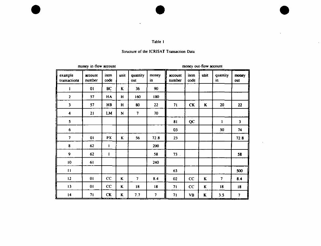
The best way to understand the transaction file is to go through a series of actual example

entries. These transactions are selected to be representative of transactions among households in

all villages. We display first a table recording actual entries, Table I, and describe each entry one

•

4

at a time. One should focus on money inflows or outflows. For this purpose we grouped

•transactions together.

aLleofamdsmt5gLicuv•

1. A household sold 36 kilograms of castor for money, 90 rupees. This is recorded as a moneyinflow into the 01 account, income from crop production (below we treat this as the sale from crop

inventory), and the quantity and value are recorded. For this transaction there is no money

outflow, and no numbers are recorded.

2. A male member of the household supplied 160 hours of labor and got paid 180 rupees, amoney inflow into account 57, income from labor supply. There is no entry in the money outflowaccount.

3. A female laborer supplied 80 hours of labor and got paid in paddy (high yielding variety). The

market value was 22 rupees. This barter transaction is recorded as a money inflow in the labor

account, again account 57, and a money outflow from the consumption account 71, as if

repurchasing rice.

4. Seven sheep were sold for cash, 70 rupees. This enters as a money inflow into account 21, ,(sale) of production capital.

Expenditures on Goods and Services5. The purchase of kitchen utensils at 3 rupees is treated as a simple money outflow from theconsumer durable account 81.

6. The purchase of fertilizer at 74 rupees is treated as a money outflow from production account

03.

7. A share rent was paid in pulses, 56 kg. This is treated as a money inflow from sale of pulses,

72.8 rupees in value, from the crop production account, and a corresponding money outflow,

again 72.8 rupees from the production capital account 23.

Financial Transactions8. A household borrowed 200 rupees in cash. This is recorded as a money inflow into account

62, financial assets - credit, savings, and gifts.

9. The household borrowed goods (medicines, cosmetics, soap, or barber services), 58 rupees in

value. This is recorded as a cash inflow into the financial asset account 62 matched with a cash

outflow into a category of nonfood consumption, account 73.

10. 240 rupees are withdrawn from a savings account. This is treated as the sale of a financial

asset from account 61, with the rupees credited as a cash inflow.

•

•

1 1. When interest is paid in the amount of 500 rupees, this is treated as a cash outflow fromfinancial account 63. •

Intra-Household Transactions

12. The household used 7 kilograms of jowar-sorghum (local variety) as seed for crop

production. The value recorded was 8.4 rupees. This is recorded as a sale from the crop income

and expenses account 01, with a cash inflow of 8.4 rupees, and also an input into the crop income

and expense account 02, with the same rupee value as a cash outflow.

13. The household milled 18 kilograms of jowar-sorghum (local variety), 18 rupees in value, for

consumption. This is recorded as a sale of output from the crop income account 01 with the

corresponding cash inflow, and also a purchase of consumption into the consumption account 71

with the corresponding cash outflow.

Darter Exchange in Consumption

14. The same household exchanged 7.7 kilogram of paddy (high yielding variety of rice) for 3.5

kilograms of spice (salt, tamarind, etc.). The imputed market value was 7 rupees. This transaction

is recorded as a sale of paddy from the consumption account, 71, with a money inflow of 7

rupees, and quantity and value of rice is recorded. This is also recorded simultaneously as a

purchase of spice into account 71, with a money outflow of 7 rupees, and the quantity and value of

spice is also recorded. The sale of paddy would be from the crop income account 01 if paddy were

not yet milled (see transaction number 1 above.) I • but when paddy is milled, it enters the

consumption account 71.

As is now evident, every market transaction can be distinguished as either a barter or a cash

transaction. This is our first basic point about the transaction file. A cash transaction, i.e., pure

sale, or pure purchase, enters into a cash inflow or cash outflow account, only. On the other hand,

a barter transaction (or within-household transaction) is entered into both a cash inflow and a cash

outflow account; the monetary values are equivalent, and indeed cash never changes hands. It is

precisely from this evident distinction in the accounts that we are able to measure the actual use of

currency in exchange (excluding within-household transactions). We shall discuss later common

patterns of monetary and barter exchange.

At this point we need to digress to a technical matter. As in transaction #1, the sale of

castor, income accrues in the transaction account only when the item is actually sold. In practice

sale may come well after harvest, and so castor would be held in inventory in the interim. We are

interested in this paper, however, not only in the use of currency but in the use of crop inventory

(and other devices) to smooth income fluctuations, so we like to record systematically the date of

•

•6

•

•

•

production, the use of crop inventory subsequent to that production, and of course eventually sale

as recorded in the transaction file. To do this we turn to the crop production file. As noted, the

crop production file records outputs on all operated plots, precisely the information we need. Thuswe added the desired entries to a new transaction account. We treat the production output at the

time it occurs as a money inflow into an unnumbered account as if immediately sold, adding torevenue, but also at the same time as a money outflow into another unnumbered account as if the

crop were repurchased and placed into inventory. Table 2 displays an example of how one can

treat recorded transactions in castor as going into or out of an inventory account.

Related, we are aware of alternative ways of treating crop expenses. For example, we

could have taken the purchase of a crop input in the transaction file at the date of purchase and

distinguished this from the date of its use in the production file. We could, in fact, create an input

inventory category. We did not do this for several reasons. First, inputs which are crops or

capital are already picked up in crop inventory accounts or dealt with in other ways (see below).

This leaves inputs such as fertilizers, pesticides and herbicides, and we think these are of second-

order importance in deficits and their finance. If we had made this change, we would then have to

treat input expenses into livestock and into trade and handicrafts asymmetrically. The only,

information we have on these types of inputs is in the transaction file; there is no separate file for

these occupations.

We now make a second point about these example transactions which brings us very much

to the issue of financing the gap between revenue and expenditures. The point is that we can write

down a transaction balance equation, and that every transaction enters this equation twice.

The transaction balance equation states that the difference in value between expendituresand revenue for some household i at date t, puta – pan, must be financed by the sale of real

capital assets –I (K0, – Kur)pku; the sale of crop inventory, – pa(Stu – Su); the use of previously1=1

acquired cash, –(M tu – Mu) ; or nominal borrowing plus gifts, –(13'a – Bu). That is,

( 1) purCu – pan = (tug – ICOptit – pd(SC – Su) – (MC – (Bt -

To utilize equation (1) we need to categorize transactions. For example, the term purCu for

expenditures includes all nondurable consumption items including rent; all noncapital inputs into

crop production, into trade and handicraft, and into livestock; all capital and durable goodmaintenance items; and similar noncapital expenditure items. The term pan for revenue includes

value of crops at the time of production (which again we treat as a sale to another household or to

an inventory account), the value of trade and handicraft products sold, the earnings from wage

labor, sale of products from livestock, and the sale of certain consumption goods (see above).Note the term AC. – putYu appears in the notation as the difference between consumption and

income, but in fact we use it more generally to mean the difference between revenues and

expenditures of all kinds. For example, input expenditure might logically be subtracted from the

value of crop output, but we treat it equally with consumption expenditures.

More specifically, the term –ye– Kw)pko is the sale of real capital, consisting of theI-1

sale of consumer durables, livestock, jewelry, land, farm equipment, buildings, and pumps. Theterm –pri(S'a – Su) is the sale of crop inventory. The term –(BC– By) is borrowing, reduction of

savings accounts, incoming gifts, and receipt of stolen goods. Note finally that any of these sales

or reductions can be negative, in which case they represent purchases, accumulation of assets, and

so on.

We now come back to the point that every transaction enters the transaction balance

equation (1) twice. In transaction number 1 above, the sale of goods represents both a reduction in

crop inventory and an increase in cash holdings. That is, the transaction enters with a negative and

a positive sign, and in the same amount, on the right-hand side of the transaction balance equation.

This is a kind of portfolio shift. The labor supply transaction number 2 enters as a revenue on the

left-hand side and an increase in cash holding on the right-hand side. The labor barter transaction

number 3 represents both revenue and consumption expenditures, both on the left-hand side.

Transaction number 4 is a reduction in capital assets and an increase in cash holdings, again a

portfolio shift. Transaction number 5 is the purchase of a capital asset (consumer durable) with a

reduction in cash balances, a portfolio shift. Transaction number 6 is an expenditure (on crop

inputs) on the left accompanied by a reduction in cash on the right. The share rent in transaction

number 7 represents both revenue (from the sale of crop as in transaction number 1), and an

expenditure (for production capital), both on the left-hand side. The borrowing of money in

transaction number 8 is a decrease in a financial asset matched with an increase in cash holdings,

again a portfolio shift, but the barter-borrow transaction number 9 is a consumption expenditure on

the left with an increase in net indebtedness on the right. In financial transaction number 10 the

withdrawal from a savings account is a reduction in financial assets on the right is matched with an

increase in cash balances, and in number 11 a reduction in cash reduces net indebtedness. The

intrahousehold transactions number 12 and 13 both represent a reduction in crop inventory on the

right-hand side matched with an expenditure (on either seed or consumption, respectively) on the

left. Finally, barter transaction number 14 represents both a revenue and an expenditure on the left

side of the transaction balance equation.

The transaction balance equation deals with observed, reported transactions as picked up in

the transaction file, plus our modification for delayed sales. It does not track the changes, quality,

or value of physical or financial assets between transactions, so to speak. For example, births of

animals are conceptually identical with crops coming from seeds, and we might well have treated a

•

•

•8

•

•

•

birth as a revenue when it occurs, accompanied with a corresponding increase in livestock holding.

Deaths would be treated the same way with the opposite sign. Births and deaths are recorded in

livestock file, but we have decided not to use these data. The effect would have been to make

changes in revenue more frequent, matched with equivalent changes in real capital assets. Related.

we could have tried to make adjustments for depreciation of capital assets as well as for capital

gains. In this case, though, we do not have any direct measurement and would need to turn to

educated guesses and/or to the stock inventory file (discussed momentarily). 2 Similarly, the

incurring of a debt, or the adding of accrued interest, would be a kind of expenditure matched with

an increase in net indebtedness, but we do not see these underlying commitments in the data.3

There is an asset or stock inventory file available in the ICRISAT data. Households were

asked at the end of the crop year, approximately July 1, the amount of grain held in inventory, net

indebtedness, the value of livestock holding, and so on. We have taken a close look at these data

and compared them to data from the transaction file. For the reasons noted above, and perhaps for

other reasons, the change in the value of these assets simply fails to track the annual deficit (or

surplus) by the standards we report momentarily. This is true of all categories: changes in financial

indebtedness, changes in crop inventory, and changes in livestock. We thus focus in the rest of,

this paper on the transaction file (with one exception below).

In the following section we exploit the fact that all transaction in the transaction file enter

equation (1) twice to get an exact decomposition of budget deficits. That is, the accounts all

balance, and there are no residual errors (which we could attribute to unmeasured use of currency

or some other object). Thus one is left with the impression that all the numbers are exact and

accurate, but this is obviously not the case.

To see this point, suppose that consumption is bought with money in the market and thatthe quantity of consumptions, Cu , and the decrease in cash holdings, –( Wit – M.), are measured

with random errors as follows.(2) C:

(3) –(MC – MO= –(MC M.)*where C and the –(Ma–Mu) * denote the unmeasured true consumption quantity and the

unmeasured true decrease in cash holdings, respectively, and where the etc and vs are random

measurement errors.

Substituting (2) and (3) into (1) gives us

(4) pc,C, + Are. - perY. = – – ICOpeit – pa(SC – Su)– (MC – Mu)* + (13'a – Bu)1=1

Suppose, for example, a transaction (cash purchase of consumption) is under-reported in the

data. Then, the associated measurement error in consumption, co, is negative. This also means a

reported decrease in cash holdings which is smaller than the true amount the error 'Du is also

negative. Indeed, the measurement errors, pned and , are exactly the same. Therefore,

equation (4), the measured version of equation (1), restores the accounting identity.The same kind of reasoning can be applied to every transaction in the data. Every reported

transaction enters equation ( I) twice, so measurement errors cancel out. This is also the case forthe un-reported transactions since they are extreme cases of the under-reported transactions. Butover-, under-, and un-reported transactions should give one pause in taking all measuredtransactions in equation (1) as literally true.

Measurement error in the transaction file determines how accurate the entries in equation (1)actually are. For instance, one might ask whether people accurately recollect all previoustransactions in monthly interviews. Concerning this, there is indirect evidence for the accuracy ofrecollections: people often report multiple transactions of the same type in each interview. InAurepalle village, of the total 78,650 transactions reported, there are 9,622 cases with multiple

entries of the same type in the same month. For instance, household number 50 in Aurepallevillage reported the purchase of other spices (including sale, tamarind, etc.) seven times in June,1976. The money values of those transactions were 10, 8, 5, 6, 2, 5, and 5 rupees, respectively.

One error of which we are aware is a dmp off in measurement of certain consumption itemsin the last three years of the ICRISAT data (see table in Townsend (1994)). Thus, expendituresare understated on average and, from looking at the graphs, we conjecture that currencyaccumulation is overstated. We thus drop the last three years from the analysis below. There arealso concerns expressed by ICRISAT staff that the first year may also be less reliable in measuring

consumption from own grain stocks, and so to be safe we drop the first year also. We are left with

six years and 72 months of annual and monthly data, respectively.We are not unaware of a second, peculiar feature of the ICRISAT consumption and income

data, namely average annual income over all sampled households in any given village is abouttwice the size of average annual consumption. Perhaps consumption is under-reported, though inthis case, using only six years of data, we do not know the source of the bias. Again, the accountshave to add up, and the apparent savings show up in apparent accumulation of currency, cropinventory, and/or financial assets. We note, however, that actual measurement may be more or

less accurate. These ICRISAT villages experienced a drought in 1974, just before the survey

began, and on the other hand, experienced a drought in 1987, and in 1988, after the survey ended.

It is not inconceivable that the villages were replacing diminished stocks in anticipation of(expected) future disasters. More on this below.

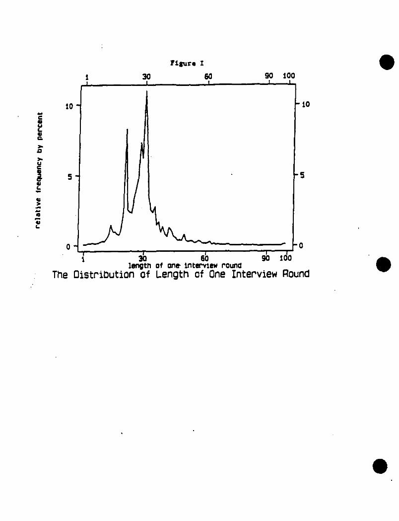
A final issue has to do with time aggregation. Our starting point is the length of interviewrounds. We cannot disaggregate any further than this recall period. We also note another sourceof error, however. Most interviews take place every four weeks, but not always. Figure 1displays the relative frequency of the length of interview rounds, and it is apparent that some

•

•

•10

•

•

•

households on occasion get interviewed earlier and some later. This makes so-called monthly data

noisy; certain monthly patterns in actual transaction may be slightly obscured. This does not affectthe financial decomposition, however.

In addition to presenting the "monthly" data, we present annual data which aggregates from

July 1 to June 30, an ICRISAT crop year. These are the years of the consumption and income data

which have been analyzed so closely in earlier work. Obviously, one of our interests is how the

measured difference between annual consumption and income is actually financed. We also

compare differences in financing in the monthly and annual data. For example, it might be thought

a priori that cash would have a high velocity. That is, that cash received from sale of crops or

other items would be used relatively quickly for purchases of other items. When aggregated over

longer intervals, more and more transactions should "look like" barter transactions in that in the

end cash balances remain unchanged. That is, annual data would not represent well the use of

currency in transactions but rather the use of currency as a store of value, if currency shows up at

all,

3. STORES OF VALUE: DECOMPOSING THE DEFICITWe began our analysis by looking at time plots of the deficit, expenses minus revenues„

against each of the four "financing" mechanisms: decrease in crop inventory, decreases in money

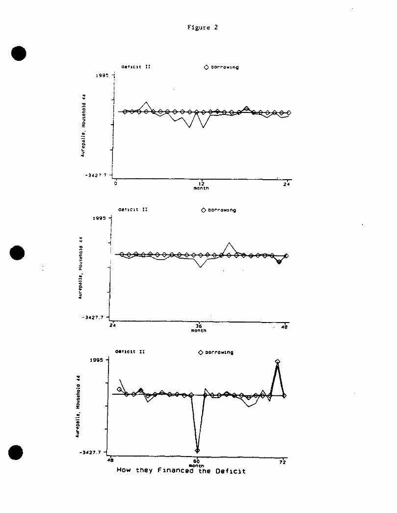
holding, reductions in financial assets, and reduction in real capital holdings. We present patterns

of each of the first three in Figures 2, 3, and 4, one household and one device at a time. We

wanted a measure which would capture the extent to which any one, or any combination, of these

mechanisms comes close to tracking the deficit numbers. Our preferred measure is a measure of

relative mean squared error, and we present this first.

For purpose of exposition let d, denote the deficit at various discrete dates t and let rn,

denote the corresponding decrease in currency balances. We take our measure of "tracking" of

cash balance reductions to be

E (di – nu)2 / Tt=1

X (c102 / Tt.,

where T is the number of observations. The numerator is the mean squared error in tracking, andthe denominator scales the numerator by the total variation of the deficit, essentially the mean

squared error when monetary changes are forced to be zero, as if money were not in the model or

as if that particular smoothing mechanism were not available to the household. Our measure is

obviously zero when monetary changes track the deficit perfectly, when the deficit is exactly

matched with a decrease in currency, (m representing changes in inventory comes close to this

standard in Figure 4, for example). Our measure is one when monetary changes are essentially

11

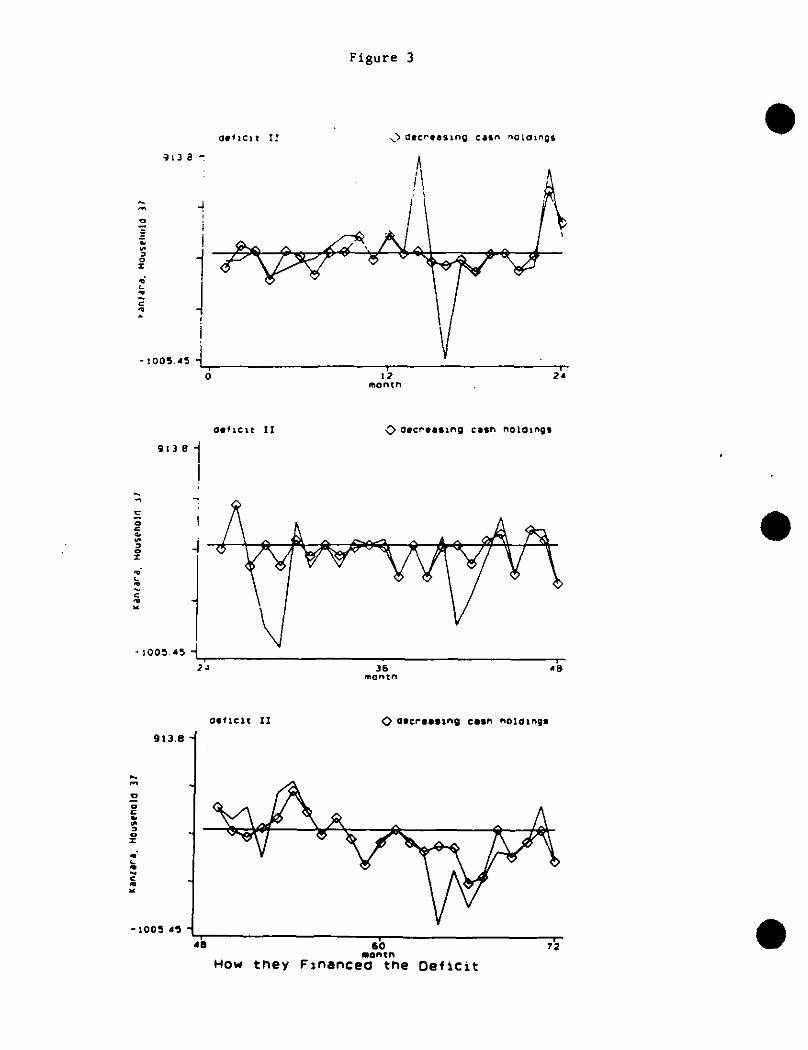
zero all the time (e.g., m representing changes in financial assets lies almost entirely on the x-axisin the first 24 months of Figure 2). If monetary changes amplify or overshoot the deficit, e.g.,accumulating money in a bad year, then the numerator is larger than the denominator and ourmeasure is greater than one minus, (e.g.. when the deficit and the smoothing device lie on oppositesides of the x-axis as in month 2 of Figure 3).

This measure of tracking is close to a measure of (I – R'), one minus explained variationrelative to total variation, with these exceptions. First, we are not finding the "best fit" of a linethrough a scatter diagram. Second, and related, we care about levels, not just comovement, and sowe do not subtract means from any of the variables.

We have also explored a more conventional measure of best fit, namely correlationcoefficients. A correlation coefficient can be high if movements in m are a scaled down version ofmovement in d, even though m does not track d well in the sense that there is a gap between thelines of the graph in Figure 2, for example. Most of the results of our paper carry through withthis alternative measure of smoothing, but our concern with levels leads us to focus in this draft onour relative mean squared error (RMSE) criterion.

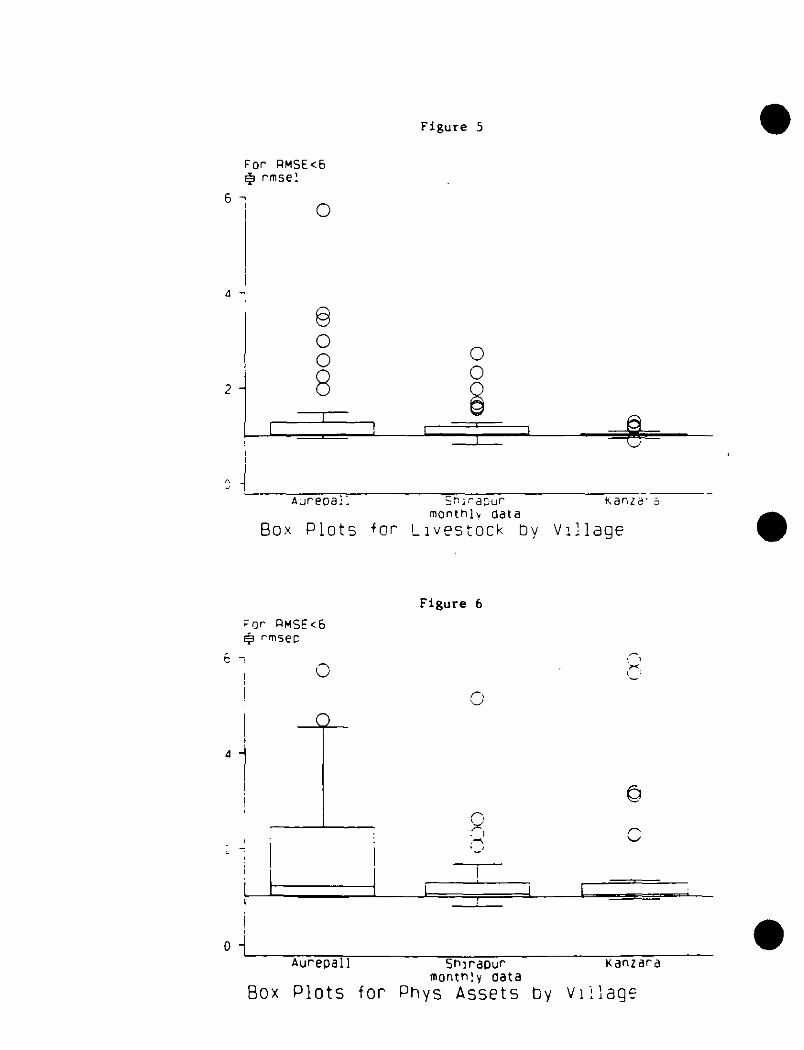
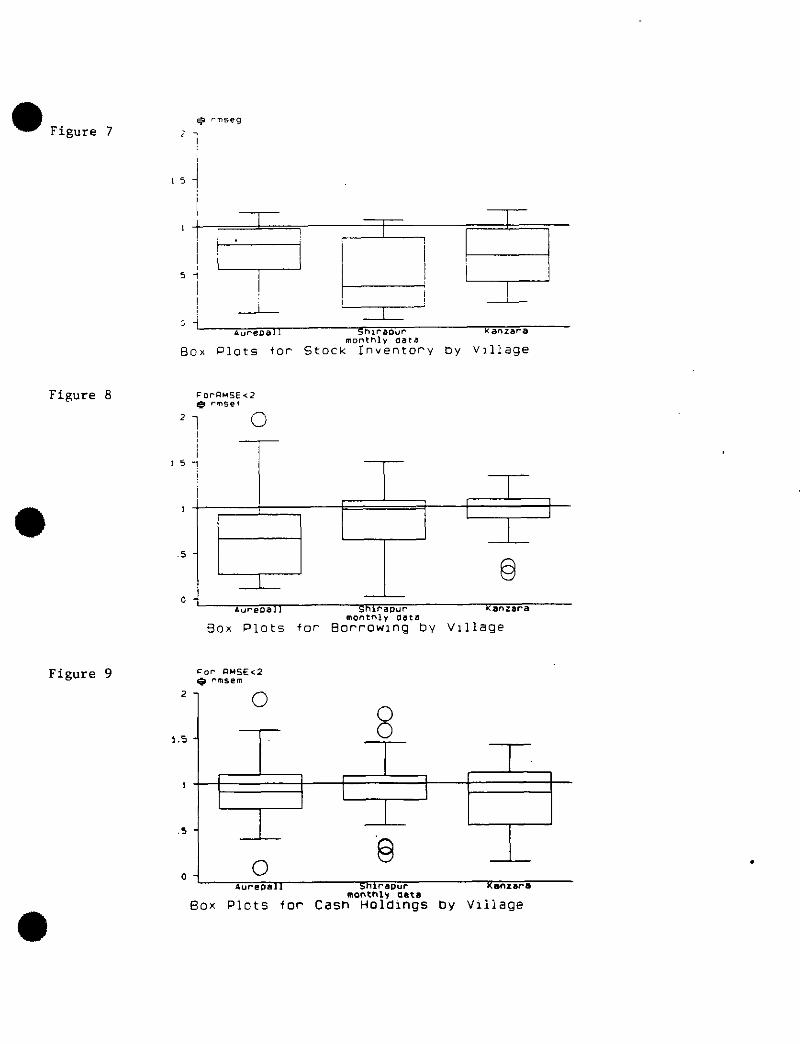
A first issue to be settled is whether real capital assets, inclusive of livestock, help or hurt.in stabilizing the deficit, so to speak. with sales in months when expenditures exceed other sourcesof revenue. To do this we use our relative mean squared error criteria where the variable m ischanges in livestock, or more generally, changes in real capital assets. To reveal some of thecharacteristics of the household-by-household distribution, we plot a Tukey or box and whiskersdiagrams, revealing the median value among households, the upper and lower quartile valuesamong households, and the maximum and minimum values of the household distribution. Thoseoutliers in distance greater than or less than 150 percent of the width of the interquantile box arealso reported. Indeed, extreme outliners can compress the scale of the graph, so sometimes theseare suppressed. If they are, the graphs themselves indicate the cutoff value, on the y-axis. Oneach graph we plot separately each of the three villages.

Figure 5 and 6 are thus Tukey diagrams of livestock and real capital assets, respectively,using monthly data. As is evident, for all real assets, the RMSE criterion exceeds one for virtuallyall households. Thus asset transactions actually "destabilize" the deficit, with purchases in badmonths, and sales in good months, for example. The same is true for livestock with the exceptionof the lowest quantile of households, and even for these households the RMSE criterion is stillrelatively high. Hereafter, in presenting the statistics for monthly data, we shift real assetpurchases and livestock to the left-hand side of equation (1), as "contribution" to the deficit, e.g.,purchases contribute to the deficit and sales to a surplus.

The measures of the tracking of the monthly deficit after real asset changes are presented inTukey diagrams, village by village, in Figures 7, 8, and 9 for crop inventory, credit cum gifts, and

•

12

•

•

•

currency, respectively.' By far and away the most evident feature of the graphs is the extensive

use of crop inventory as a smoothing device across all three villages. The interquantile range in

Figure 7 lies entirely below unity for all three villages. This is not the case for credit cum gifts in

Figure 8 nor for currency in Figure 9. Clearly crop inventory is a salient smoothing device, as

Paxson and Chaudhuri (1994) suggest.

There are patterns by village, however, in the relative (and absolute) use of financing

mechanisms. Figure 8 for credit shows that Aurepalle households use this device in larger

numbers than in either of the other two villages, though Shirapur households did use this device.

Indeed, credit does better in absolute terms in Aurepalle than does stock inventory. (Compare the

distribution in Figure 8 with the distribution in Figure 7, with the exception of the highest quartile.)

Figure 9 for currency shows that Kanzara households use this device in larger numbers than in

either of the other two villages. In this case though, stock inventory does better in Kanzara in

absolute terms. Compare the interquantile range in Figure 9 with Figure 7 The role of currency in

Kanzara is consistent with the results of Paxson and Chaudhuri (1994), but the role of credit in

Aurepalle and Shirapur is not.

Again, Figures 2, 3, and 4 present various time series graphs for various selected,

individual households which fit these salient patterns: credit only in Aurepalle, currency only in

Kanzara, and crop inventory only in Shirapur,. For each case we present one household which is

at the lowest (best) quartile, that is, the graphs of 1/4 of the households in that village would

appear even tighter, with better tracking. The reader can judge visually just how closely each

device is tracking the deficit for RMSE numbers of .5429, .2850, and .1425, respectively. On

occasion the fit is remarkable - e.g., inventory in Shirapur.

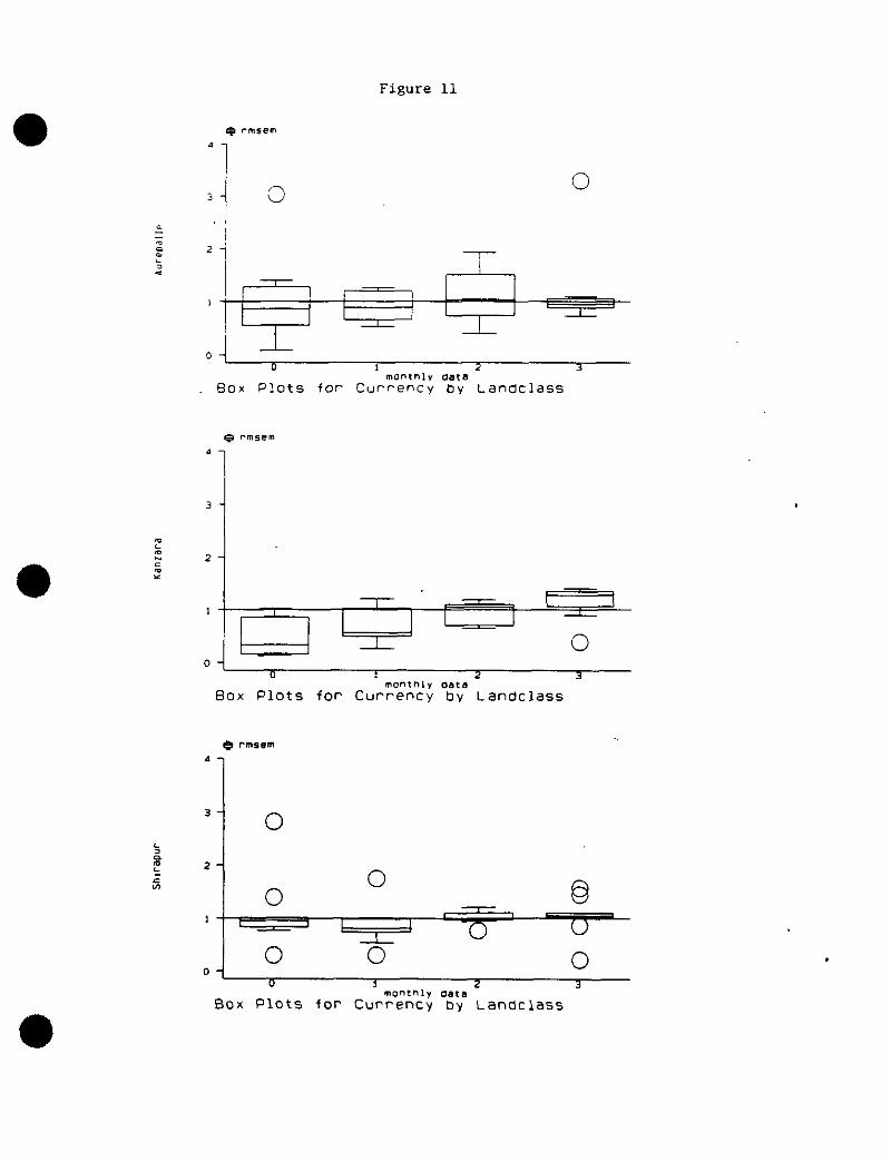
There are striking patterns by landclass for some smoothing devices, though the sample is

small when stratified in this way. Recall there are roughly 10 households in each class, coded 0,

1, 2, 3, and for landless, small, medium, and large landholders, respectively. When restricting

attention to inventory only, it seems to be the larger landholders rather the small or landless

households who use crop inventory to smooth. See Figure 10. On the other hand, the landless are

more prone to use currency, especially in Kanzara and Shirapur. See Figure 11. There seem to be

no patterns as regards the use of credit, however, despite the fact that Townsend (1994) and

Morduch (1990) have shown the poor to be less insured or to be credit constrained, respectively.

Indeed landless and small landholders seem to use substantial amounts of credit and gifts in

Aurepalle and Shirapur. See Figure 12.

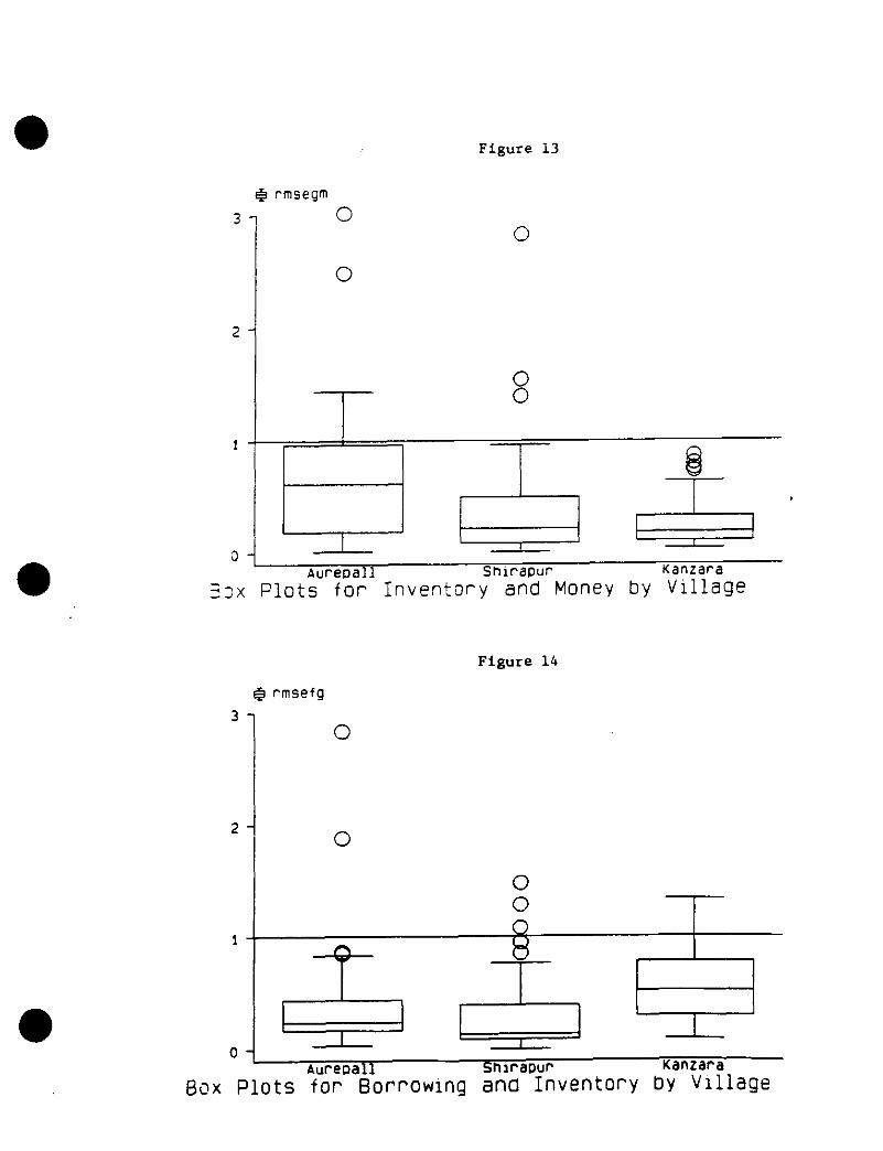
One can also examine the effect of various combinations of mechanism. Of immediate note

is that the sum of mechanism will almost inevitably do better than any one mechanism individually.

Note in Figures 13 and 14 how the Tukey diagrams are below unity, whereas earlier portions were

above, for example. Indeed, by construction, all three mechanisms track the deficit perfectly --

13

everybody would be piled up at zero! Having said this, we can compare across villages and note

that money and inventory act well in combination with each other in Shirapur and Kanzara in

Figure 13, but less so in Aurepalle where, as noted earlier, credit (the left out mechanism) plays a

salient role. Related, credit and inventory play salient roles in Aurepalle and Shirapur in Figure 14,

but less so in Kanzara where currency (the left out mechanism) plays a salient role.

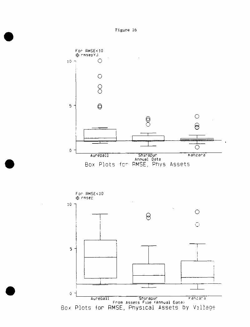
Turning to the annual data we come again to the issue of whether livestock, or real capital

assets in general, "stabilize" the deficit. They do not for three fourths of the households. We

report in Figures 15 and 16 here from the transactions files, aggregating months into years, the

Tukey diagrams for livestock and real capital assets, respectively. We report here as well the

corresponding diagrams when we use the asset/inventory files. There is little improvement. (The

figures for stock inventory and for financial assets from the asset/stock inventory files also show

little smoothing - available on request.)

Otherwise the annual diagrams mirror what we learned earlier in the monthly data, with one

exception. While Shirapur relies relatively more on stock inventory in Figure 17 and Aurepalle

relies relatively more on financial credit cum gifts, in Figure 18, Kanzara does not rely relatively

more on currency, in Figure 19, as if the velocity of money were relatively high. In fact Aurepalle

is the heaviest use of currency in the annual data, a significant smoothing device! Introspection

about high turn over and a presumed high velocity of money would have led us astray. (Annual

data reinforce though the relative roles of currency among the poor and stock inventory among the

larger holders.)

4. TRANSACTION PATTERNS: BARTER VERSUS MONETARY EXCHANGEWe have done some preliminary work to try to see if these village economies are heavily

monetized in transactions or whether there is still a role for barter exchange. To do so, we have

disaggregated the categories of commodities further: money, IOU's, grain, other crops, food other

than crops, clothing, other consumption goods, labor, livestock, physical real assets, jewelry,

consumer durables, and a residual other category. We restricted attention to monthly data with the

idea, of course, that we care about the objects used in each and every transaction -- we do not want

to aggregate. Also, we are using the measured data from the transaction file and not our addition

from the production file. We also exclude measured intra-household transactions, that is, we are

looking at "market" transactions only. However, we do add up here over all transactions of all

sampled households in all of the six years. (Individual tables are available on request.)

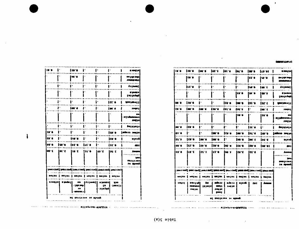
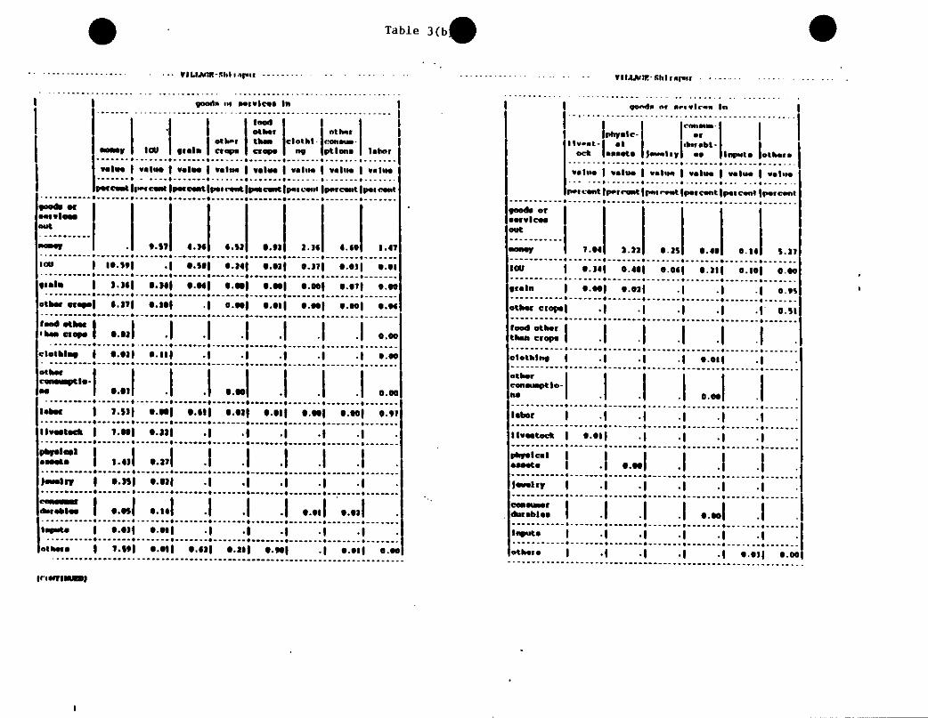
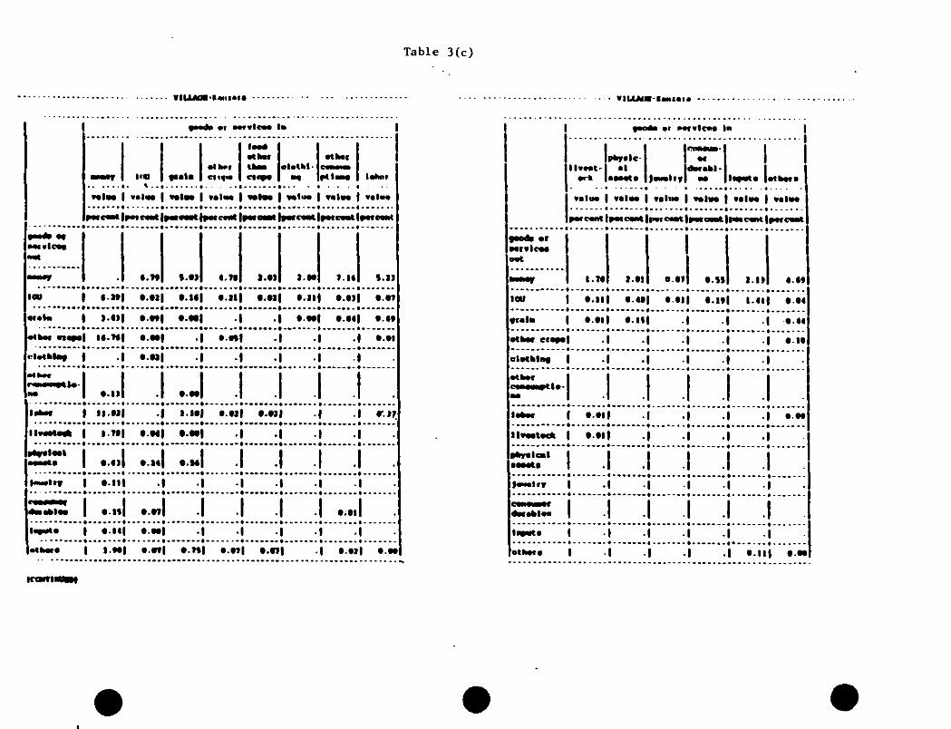
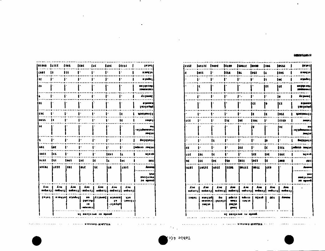
Table 3, a, b, c, present exchange patterns of each commodity against every other

commodity, including the same commodity aggregate. The entries are expressed as a percent of

the rupee value of all transactions of the village. For the record, the total rupee value in Tables 3 is

2,566,369 in Aurepalle, 4,150,772 in Shirapur, and 3,319,781 in Kanzara. Most evident in

Tables 3 is the relatively high percent of transactions by value in which currency appear in

•

•

•14

I

•

•

exchange. The first row is currency spent to purchase something, including the purchase of IOU's

(lending), and the first column is currency received from selling something, including the sale of

IOU's (borrowing). We note that in Aurepalle the rupee value of all cash purchases, including

lending, is 37 percent of the total, whereas in Shirapur and Kanzara it is 45 and 46 percent,

respectively. Thus Aurepalle is less monetarized than the other two villages. Cash sales are 43,

46, and 45 percent in Aurepalle, Shirapur, and Kanzara, respectively, a less striking difference.

That currency appears so frequently in exchange would suggest something special about currency,

that it dominates other commodities in exchange characteristics or, more crudely, that it facilitates

exchange in the sense of Clower.

The second row and second column of Table 3 are each filled with nonzero entries, in most

cases, indicating the importance of borrowing and lending (with gifts) in the three village

economies, roughly 9 - 14 percent for borrowing and 7 - 13 percent for lending. By this standard it

would seem to be inappropriate to view these village economies as rigid cash-in-advance

economies. Most expenditures, including consumption expenditures, can be and are often

financed with credit. Though we provide no table here, this is true as well when attention is

restricted to landless households even though, as noted earlier, currency may play a relatively large ,

role in smoothing monthly (and annual) fluctuations for them. Finally, we note the relatively large

role of grain loans in Aurepalle, the less monetized village economy where the role of credit was

noted earlier.

There are some relatively large entries other than in the first two rows and columns of Table

3. One of these is sale of labor for grain and to a lesser extent, for other crops and for other

consumption items. The other side of this transaction is grain sold for labor. Obviously, landless

laborers and many small farmers are on average providing labor to medium and larger landed

households for grain. This is confirmed when we distinguished the tables by landclass, but again

we do not display these. Another nontrivial entry in Aurepalle, but not the other two villages, is

the exchange of jewelry for other consumption goods. Such entries display the common types of

barter exchange. We would have to say that the village economies are mixed economies,

displaying both monetary and barter exchange.

There are some nonzero entries on the diagonals of Table 3 of some interest. One is labor

for labor, another is livestock for livestock. We strongly suspect these are exchange transactions in

which households take turns helping each other out in crop operations, requiring labor or plow

animals. (We do not interpret grain for grain.)

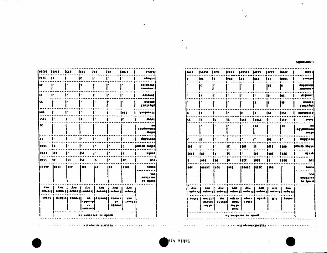
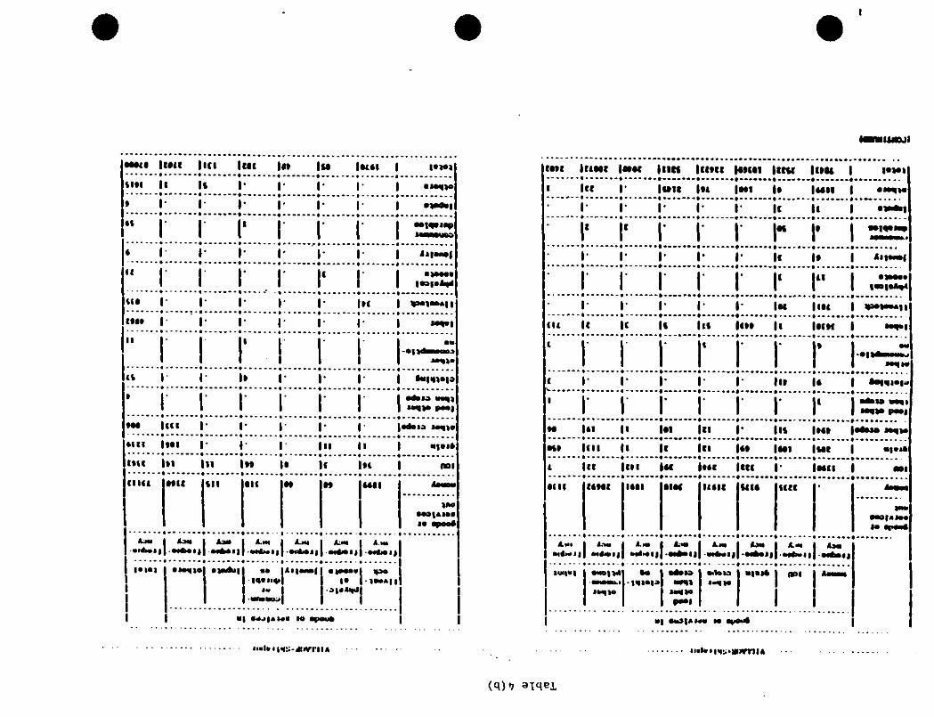
Another closely related view of transactions is presented in Table 4, a, b, c -- a simple

count of the number of transactions, not aggregated in value terms. We note, for example, by this

new standard that the relative importance of credit drops somewhat; less than 5 percent for

borrowing and less than 5 percent for lending in all three villages. Obviously, credit transactions

15

are lumpy. that is, they tend to be large by value when they occur. Apparently, there are

"transactions costs" even within these village economies in the use of credit. We wonder what

these are.

Finally, we would like to take these transactions data further and trace out typical

transactions as in the models of Jevons (1875), Kiyotaki and Wright (1989), and Banerjee and

Maskin (1996), for example, that is. with something purchased from one person and then used

later in a sale to another. The evident problem with this is that virtually all objects can be and often

are held in inventory simultaneously, over many periods, so it is difficult to identify the original

source of the object used in exchange. Further, there is some consumption between exchanges.

Finally, currency and commodity barter coexist. The bottom line is that the simple (but not easy to

analyze) models of exchange in the literature are contradicted by salient facts. Currency, in

particular, is both a store of value and a medium of exchange.

5. SPATIAL PATTERNS: MICRO FOUNDATIONS FOR MACRO MODELSWe are not unaware that the essence of monetary theory is to deliver valued money in an

otherwise closed economy. What is it in the economy as a whole that gives rise to fiat currency,for example? Needless to say, these ICRISAT village economies are not closed economies. They ,

may be using currency to facilitate transactions and store value because currency is valued in the

larger national economy of India. Viewed in this way, transactions within a village cannot shedsufficient light on the essential impediment to trade which gives rise to valued money in the larger

national economy.

Nevertheless, the relationship of these village economies to the larger national economy isnot without interest to monetary theorists. We might view the village as solving its own optimum

problem among various diverse households, perhaps approaching something resembling a within-

village Pareto optimum. This is the case in the model of Manuelli and Sargent (1994), for

example, putting cross-household diversity in the model of Townsend (1980). Again, the

evidence for an internal Pareto optimum within the ICRISAT village economies is not wildly

inconsistent with this standard; see Townsend (1994). But in its relationship to the larger national

economy, the village may act as an aggregated consumer (even if preferences do not aggregate),

using currency, crop inventory, and (limited) credit to smooth fluctuations; see the exposition in

Townsend (1995). The work of Deaton (1989) would suggest, in particular, that savings play a

buffer stock role.

The issue is not what transactions take place within a village or outside a village; if markets

function well and local transaction costs are small, internal village prices are driven to external

regional prices, and each household would be indifferent to supplying labor in the village or

outside it, for example. Labor could be hired in, could be financed with labor exports, for

example. We thus add up among all transactions for each household and then add up transactions

16

•

I

•

over all sampled households in each village. This allows us to see how each village is financing itsaggregate balance of permanent deficit. In doing so we are aware of one problem: in Aurepalle animportant group of local lenders was not included in the ICRISAT sample of households, thus so-

called aggregate deficits in Aurepalle may be financed by within-village lenders, not by the outside

economy.

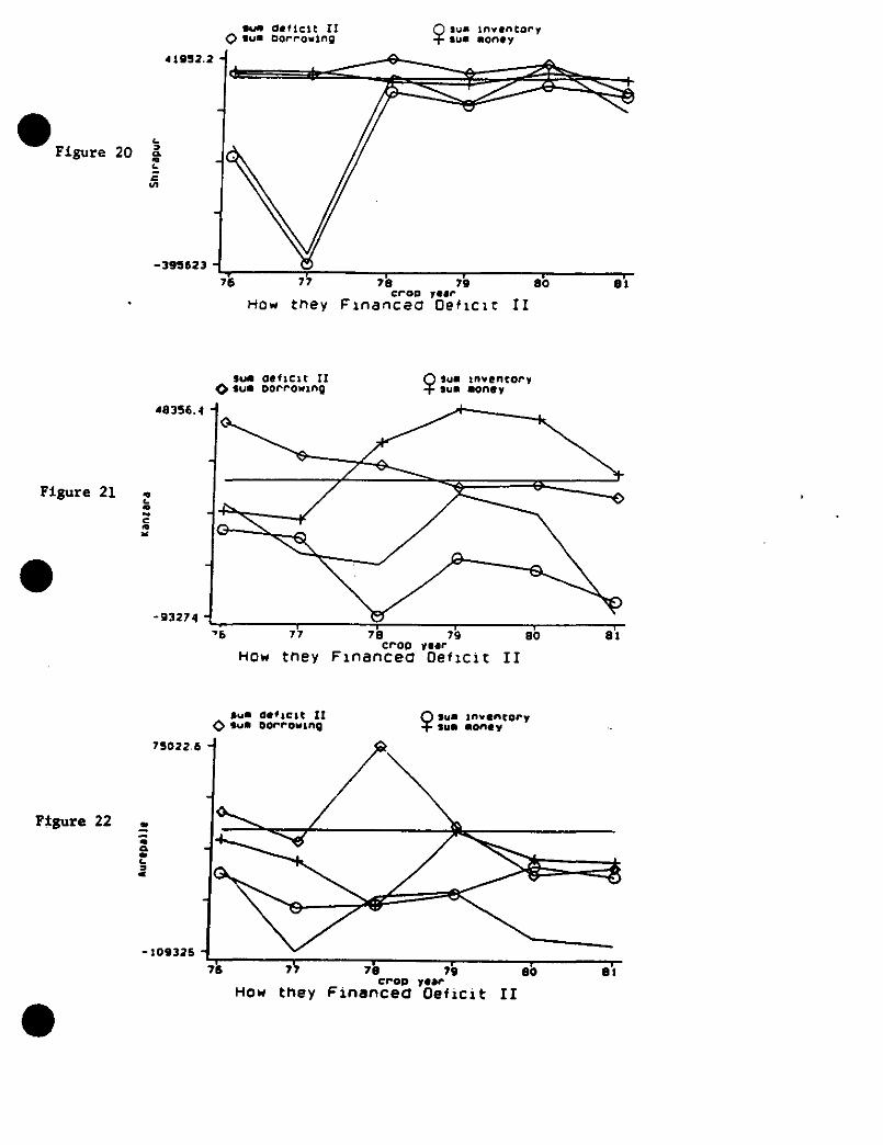
What then are the roles of credit and currency? In Shirapur's annual data these objects play

little role (see Figure 20), but in Kanzara and Aurepalle their roles are as large in absolute value as

the size of the surplus (see Figures 21 and 22). It appears, however, that currency and credit are

offsetting one another, with movements at times unrelated to the surplus itself.

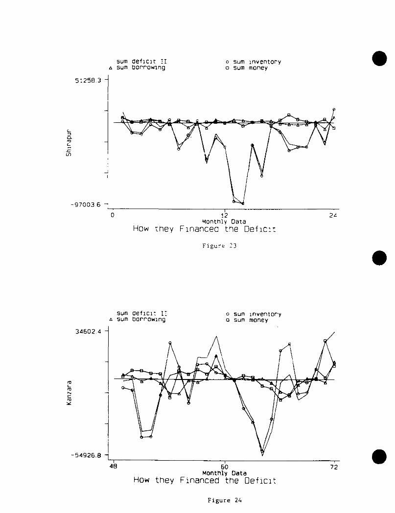
These patterns, though less evident, are present in the monthly data. Shirapur's use of

crop inventory remains dramatic; see months 0 - 24, in Figure 23. Kanzara's use of crop

inventory is also evident; see months 48 - 72 in Figure 24, but credit and currency are playing a

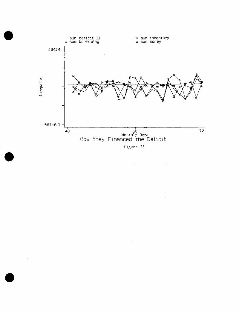
more salient if unrelated role. Finally, Aurepalle's use of crop inventory is much less evident; see

months 48 - 72 in Figure 25, with currency and credit playing large if erratic roles.

In conclusion, models of village economies which ignore outside credit would seem to go

astray. This is consistent with the work of Rosenzweig (1988), describing the role of remittances

and marriages, for example. Nevertheless, outside financial assets are a limited device when it

comes to smoothing village consumption. This is consistent with the view often expressed in the

literature that within-village credit markets may function well, due perhaps to an information

advantage, and external credit markets do not function well, because they are more distant from

local borrowers.

The role of currency in smoothing village-level fluctuations is problematic. In Shirapur this

role is small, but in Aurepalle and Kanzara the role of currency can be as large as the role of credit.

Still, as noted, currency and outside credit seem to be substitutes for one another in the sense that

one goes down when the other goes up. Perhaps the villages are solving some kind of portfolio

management problem. The relatively simple (but not easy to analyze) turnpike models appear to be

missing much of the complexity of village-regional interactions.

6. CONCLUSION

We are not unaware that the results of the paper beg further model construction. We now

know, subject to measurement error, that there are salient patterns in the use of currency and crop

inventory by land class and that the relative importance of currency, crop inventory and credit

varies within and across these villages economies. In two of the three villages, credit and

insurance play an important internal role, but simple permanent income or full insurance models are

rejected in the consumption and income data. Intermediate private-information models seem to fit

the consumption-income data best, but existing models need to be altered to allow nontrivial

discretion on the part of individuals in the use of currency, assets and/or credit cum gifts, in the use

17

of these to smooth consumption intertemporally. Credit also plays a role in financing asset

purchases and sales, and this also begs a model. We also need to model better observed patterns

of exchange. to get at the costs and benefits of barter and credit as they compete with the role of

currency as a media of exchange.

•

•

•18

• Endnotes1. The sale of paddy would be from the crop income account 01 if paddy were not yet milled, as

in transaction 13, but milled paddy is sold from the consumption account 71. Consumption of

paddy used in other papers, e.g., Townsend (1994), represents all paddy milled in a given month

plus purchases of milled paddy less sales of milled paddy. To the extent that paddy is milled in one

month but sold in another, this procedure overvalues consumption in the first month, and adjusts it

later. The problem is that there is no measure of milled grain held in inventory, neither in the

original ICRISAT data, nor here, below, when we construct our crop inventory account.

2. The example of transactions in castor is now seen as misleading as it did not allow for

depreciation; if the transaction had been recorded in value terms, it would not have allowed for

price changes.

3. A related point: loans are often forgiven and we do not see this either.

4. If we do add real asset purchases to the deficit, then the other smoothing devices track the

deficit less well. Credit in particular does worse, suggesting that not a small amount of credit is

financing real asset purchases. Recall, however, that this helps to keep consumption smooth

ceteris paribus.

•

•19

References

Banerjee, A. and E. Maskin, "A Walrasian Theory of Money and Barter," manuscript, 1996.

Deaton, Angus, "Saving in Developing Countries: Theory and Review," in Proceedings of theWorld Bank Conference on Development Economics, Washington, D.C.: International Bank forReconstruction and Development/World Bank, 1989, 61-96.

Jevons, W.S., Money and the Mechanism of Exchange Appleton, London, 1875.

Kiyotaki and Wright, "On Money as a Medium of Exchange," Journal of Political Economy,97(4), 1989, 927-954.

Ligon, Ethan, "Risk Sharing Under Varying Information Regimes: Theory and Measurement inVillage Economies," 1993, University of Chicago, Dissertation.

Lim, Youngjae, "Disentangling Permanent Income from Risk Sharing: A General EquilibriumPerspective on Credit Markets in Rural South India," 1992, University of Chicago, Dissertation.

Lucas, Robert and Nancy Stokey, "Money and Interest in a Cash-In-Advance Economy,"Econometrica, 55, 1987, 491-514.

Manuelli, R. and T. Sargent, "Alternative Monetary Models in a Turnpike Economy," 1994,manuscript.

Morduch, Jonathan, "Risk, Production, and Saving: Theory and Evidence from IndianHouseholds," Harvard University, manuscript, 1990.

Paxson, C. and C. Chaudhuri, "Consumption Smoothing and Income Seasonality in Rural India,"1994, manuscript.

Rosenzweig, M. "Risk, Implicit Contracts and the Family in Rural Areas of Low-IncomeCountries," Economic Journal, 98, 1988, 1148-1170.

Rosenzweig, M. and K. Wo1pin, "Credit Market Constraints, Consumption Smoothing and theAccumulation of Durable Production Assets in Low-Income Countries: Investments in Bullocks inIndia," Journal of Political Economy, 101(2), 1993.

Samuelson, Paul A., "An Exact Consumption-loan Model of Interest With or Without the SocialContrivance of Money," Journal of Political Economy, 66(6), 1958: 467-482.

Sargent, Thomas J., "Credit and Currency with Overlapping Generations," in DynamicMacroeconomic Theory, Harvard University Press, Cambridge, Massachusetts and London,England, 1987.

Tobin, James, Discussion, Models of Monetary Economies Eds J Kareken and N. Wallace,Proceedings and contributions from participants of the Federal Reserve Bank of Minneapolisconference, 1980: 83-90.

Townsend, Robert, "Models of Money with Spatially Separated Agents," in Models of MonetaryEconomies, John Kareken and Neil Wallace, eds., Federal Reserve Bank of Minneapolis, 1980,265-303.

"Risk and Insurance in Village India," Econometrica, 62(3), May 1994, 539-591.

•

•

•20

"Financial Systems in Northern Thai Villages," Quarterly Journal of Economics,November 1995, 1011-1046.

Walker, T.S. and J.G. Ryan, Village and Household Economies in India's Semi-Arid Tronick,Johns Hopkins, manuscript, 1990.

Wallace, Neil, "Models of Overlapping Generations: An Exposition," University of Minnesota,Minneapolis, 1978.

Zeldes, Stephen, "Consumption and Liquidity Constraints: An Empirical Investigation," Journal ofPolitical Economy , 97, April 1989: 30546.

•

•21

• • •

Table I

Structure of the ICRISAT Transaction Data

money in-flow account money out-flow account

I exampletransactions

accountnumber

itemcode

unit quantityout

moneyin

I accountI number

itemcode

Sit quantityin

moneyout

I 01 BC K 36 90I

2 57 HA H 160 180

3 57 HB H 80 22 71 CK K 20 22

4 21 LM N 7 70

5 81 QC 1 3

6 03 50 74

7 01 PX K 56 72.8 23 72.8

8 62 I 200

9 62 1 58 73 58

10 61 240

II 63 500

12 01 CC K 7 8.4 02 CC K 7 8.4

13 01 CC K 18 18 71 CC K 18 18

14 71 CK K 7.7 7 71 VB K 3.5 7

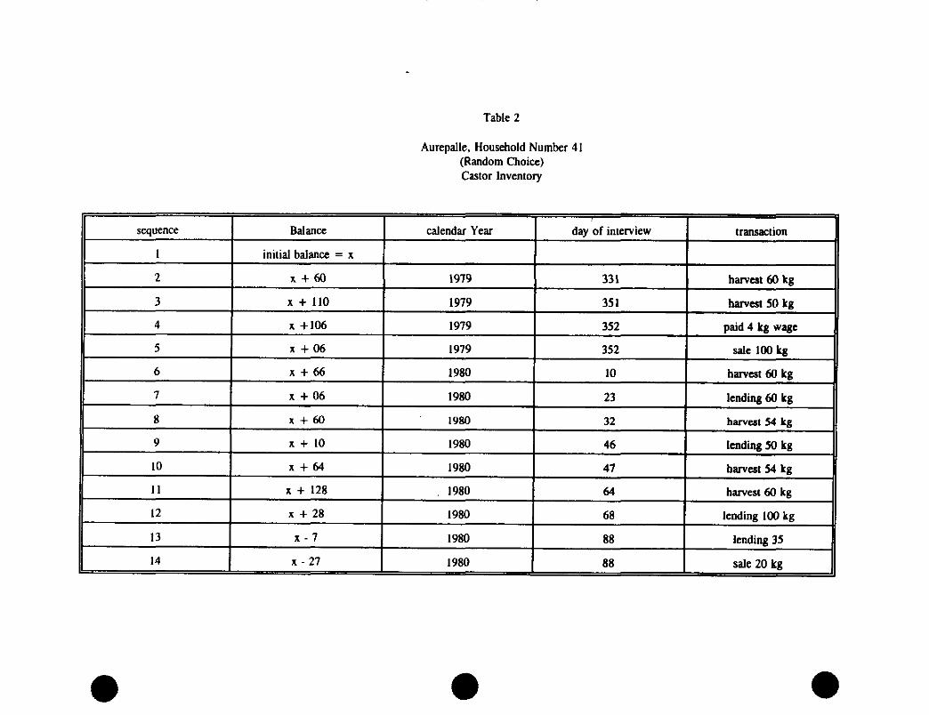
Table 2

Aurepalle, Household Number 41(Random Choice)Castor Inventory

sequence Balance calendar Year day of interview transaction

I initial balance = x

2 x + 60 1979 331 harvest 60 kg

3 x + 110 1979 351 harvest 50 kg

4 x +106 1979 352 paid 4 kg wage

5 x + 06 1979 352 sale 100 kg

6 x + 66 1980 10 harvest 60 kg

7 x + 06 1980 23 lending 60 kg

8 x + 60 1980 32 harvest 54 kg

9 x + 10 1980 46 lending 50 kg

10 x + 64 1980 47 harvest 54 kg

II x + 128 1980 64 harvest 60 kg

12 x + 28 1980 68 lending 100 kg

13 x - 7 1980 88 lending 35

14 x - 27 1980 88 sale 20 kg

• ••

• • •

10'0

IS' • I•O •

DO • S S0•1 St's a'S II•S110• 5

IS • . • sirs

• Ines

In •

I • i

Ia' t

I . I•

I

a't

IWO IIn.

11S•C

111••

•••••••••J1M.S•oa•e/

Salaini•0

want

agog

aplarma▪nano

••aagaSSW mega

magi

Ana

1.43 /a•N eat

ISIMISMI1J1

Iwo Is.. Iwo Ian In-. lays In •. lire, I •Suga • a * • • .

l in I . I. I. I.ICC'. 11.0 •. magramp

StamasaItC • 11 1' 1' l' 1' 1S•. In-s Asps, • • • I . I. I- I. Is" In. Ism . ' I

1naafi

stigma. • • • • • • owe 118'0 I• I' Kee IOU. al', Itt • t pawn' • • • • - - . CS'Il OS'. in-.ace Ism.In*. I' On I •O,Of• • • 100 C0. esammomm4

10.1.me

00 • S CO•. i■nan

01'0 • ss'il are Ore Itt's n't Inn Inn

CS • 0 Ci•S St. IO•I I•O 1.▪ 4'C 51 . 1 .1.84ore sue I •o IN .. ere cc. It• s •• own 0.1 • IS'S lutt In 1 lIt'.Itt 11'0 I MHO

.alas.opmm•

•

•%rand seandllmosadlgra ga *masa Palma tam sod we►1 ••• pease+, Wan sek•S la WIDOW •ii■J ka 4Nya/a

MICA swum 1 ago* 1 •ftlea age* magma seal OA •• Sea& MIM MIMI alga • • ••••110 sat' S. 'Aspens( ablia •ommg small. a onsa edis•a malt-gamy' a .1_A11 -OR040.1 Salsa emu Bea*so f Sad •u* Joao

-MbellaJ pal

019511 al a

ni

mg augasms se %%Me . wags... ms epos.

.......... • • •ige•leas.•-•••11111.. . ......... •II•dosIntentall • • ........

(e)£ aPie.I.

good. ot 091010011 Is goods or orevIcos In

• • porcentiporcentlimocvnt

enesooe.fores Impute LIMED

191.0101- I

1011n. vein. I Wasspotent peoceollpefeen1

Ot10.1norm, 1 1W 1 grain 1 crop, • value vela* vele* value

•percent percent percent percent yeomen percent portent praceut

foodother ether LWOW':Own cloth' . consum 1 alcrope mil otiose 1 lobar 111vool

Oct 'assets Ipmeley • voles vela* value value 11.100 I value I fable

goods Ofawakesgotemney 7.04 3.22 0.2S 0.40

•

0.14 S.271W 0.14 0.49 0.06 11.21 0.10 0.00groin 0.00 0.02 0.9Sother cropsfood otherthen flopsclothingother

1 • .01

. 0.51

consumptio-nslabor

0.00•

livestock 0.01physicalassets 0. 90 •jewelry •C0000001aerobia 0.50•Imputeothers 0.01 0.00•

goody etnovicesoutlag& . 9.57 4.70 4.42 0.91 2.14 4.60100 10.19 0.50 0.24 0.03 0.17 0.01lisle 3.16 0.34 1.1$ 0.80 0.00 0.00 0.07othef romps 6.27 0.10 0.00 0.01 0.01 0.00

1.47O.010.00O.04

/sod otherohms crape 0.01clothing 0.02 0.11

Luellaconsonstangles

1

Irevate lothers 1

othercranreptie-011 0.07labor 7.53 9.00 11.41 0.01 0.91 0.00 0.00 OAP/Ilinoteek 7.00 0.2206001001sent* 1.01 0.27

1.331 1.11 •

0.0510.000.011 0.011

• •9.991 1.011

• ••1 •

•

•

0.901•

0.011 9.92

.1

•

.1 0.01 0.00

0.000.00

0. 00

•Table 3 ( b•• •

V11.1.1111111-01.114r.•t .......... VIM/VW s61 isms -

groornal

••me4414 pelmet p6466mthmmramst goematlips4coma pelmet penal •

peceantlpoicestlp•nontt peecest poweentlpercent• • goal. ICsel•Itioeel

geode 4176611,1766mot

VILLA01otnnons

Vied,

Ised64herthe

of Der/ION S.

61.161-elber

caw..Ipkyole-

lionst- 71

VILUKR-Bal•••

goods el illertICOS

camoom-64

du4.191-

Is1

1 1olherwar I 199

t. pole I anon naps mg p11.66 1699w *rat moots loonley co IMMO Islbown

••nit* vales value value vale, value 76164 vale* Wattle I vale* VsItIO vale, vale* I VON*

11.71 3.13 4.78 •

las 6.31 6.021 0.141 0.11 • •

s•419 1 1.41 11.011 0.461

bet nap 16.76 •.11111 .1 1.01 • •

elotIblm• 1.131 .1

2.02 2.08 7.16 S.33

0.31 1.11 •.01

.1 •.011 0.84 6.68 •

.1 . 4.61

.1 •1•

..en 1.74

0.113.111 0.g1 O•SS 3.11 4.67

IOU 8.48 •.111 8.14 1.41 •.64w86e16 1.11 •.131 .1 0.44 •otter crap,

clot•ing.1.1

lie COO si ol

••••••equalort1.-

• •Intof 11.11 2.101 8.01 0.03 . 1.12

• 16464449 1.78 coal 9.1111 .1 • • • •

sots 6.41 0.341 0.16 ol Iploy01401

* • loneolig 0.11 .1 .1 -I -1 • a • • •

ebles 0.111 6.0/1 .1 .1 1 04011meaning

• • • • • loropot• •.141 8.861 •1 .1 .1• • • • ease 1 3.141 8.071 •.911 8.07 9.611 1 1.131 Ivo,

ether1 1

ommiumr11.11-asIan 6.01 •1 •,,tints! 1.111 4 •

•19761ca

.1 ol .1 .1 .1611644.8 l • ••goonlri, .1 •1 -1

• .1

• • omeammwenable. 1 •1 .1 1 .1 .1

• • imposts I .1 • • -.1 .1 • •

othors 1 .1 .1 .1 .1 8.111 0.48

•

Table 3(c)

leart10911111

• • •

11102,4106Spoo6

Lass Aar Aar Aar l Aar Aar Aar Aarsolksmi Alamos oshosj whom -NMI) sedum Amines •

amprl ouolsd 6o.Aso 1Soma ups6 nos Assam

-sow Amilecia smileMAW IMMO

FM'

II 'salsas. so .posh

lupe/

•

se gos Is►tt Iss► fit( let II, 18111 I 1•407 • • • tots It I It I* l' I' •sooso • • . . a I I II I. I. I

owns.2011111011100

LI I' I I• •I• i• l' Assert • IS

I* I* I• I' I• I sans

1•21•444•PSI I I' I' I I' IOC( I 6,61•••11 . . fist( l' l' II ;•41' IC soots

•

I . I. I I. I. I. -imams,*

awnsem(t

414 I• I. I• SuPliola • • • 6001 It I' L Soso Joao • 1661 DI SI l' t owe6661 It (1 SC s I' Sc roe •

I

In

0031A20111so post

%nosett LI 61161 Amos Sill (Pt

A3U I kw Om I tau I Las I Lau LauAmiLossi-sabsil Ambsapl .solssoll-sobsaWsobass -sslissi• • 1'101 I emus minds!! ss plogsmoll slams sae

I • IOssI•I I le -4dsA11I

Is -•onsuoa I aIsAyd

I us iso314440 lo spoo6

rilvd.lw-Sv011s • ---------

ItrnWDal

l' l' I . l' l' let

Is I' I' I' I' It let I

t Ill I: !I Ft 11: Ito Itst

. . 6 .

I ImamIt

cc Is It it lot. 4 0lice I awe

i::::::::

I . li

lustIi1I

1-essiniest:es • • .

g t I' I' tt I.HI' C Iles Is slt Int 640::::::: • • •

1611 SC V g I' III SIC lilt • • . t seg es e bet INS C lets MI . • • 661 lain Ifts Isss beat Isoc I Ott Moos

•1p•losss•i0O7116

SOLI Uses; ICC, 111161 I loss lotto Out • t lit It Roo lot hat Its lass

;

moss

•Ope)17 aTqej, •

08018 11011 1111 Inc In Is. 16/61 I . • • . . Islog ll It l' 1* l' 1 III I. .1 l .1' .1'

• 1

•I • •

I .I. II I. 1- I. ISS

10/646/6466660•m,

6614vimp880018020

6 I' i' I' 1. 1 Asi••s$ •

I . I I. I. II I. IStO I' 1' I' I- 1* 181 1 00666.11

1186 i 61' .1' •-

LS I I I:- i- I.

I 1-41.46144143 • A641

ow1' 1 88000

II

I• 80161010

I I. I I I-1 Mesa sir

80170 0001I

no ICU i' l' I 1' 1646/a Bogle • •

16111 1 1161 l' l' 1 I6/ I I Ansa • •

11111 161 In pi 1• It ft I 001 • 81/11 611

• Olt

le In

6481

00314100se mese

ASPar

Aso I Ass Ass Li

s -tall 0000.1 aeon emb.s $ .4141.6 edam' ombessAam I L'. /14 •

islet evese l

i

• •llikla

0.0800000 10 spasm

It • sobs•l•assAqd

1

es Asian( •41•44• 7/30

so .ag•/•ld-14640 I.• -180011

• ---------- 8•01A•PIS-AWITIIA

• • •

el114/111J1

'Ott 111808 INK 11188 I • • • Kits; lent hest 1 I•soo • • • Ice I' lute 181 Ins ill •14481 1 48041• 6 er e • e o 4

1 . I. 1' 1. I. lc It i

It If Is I. I. lei

It I ISIACIAIPmamma.

•6066 • • • •

• • • • I' l' 1' I. I' 11 14 I A•pm44

I. I. I. I. I. II Itt

II taint;070080 • • • •

• • • I 1 l' 1' 1' let l i st 1 66•100als • a • • • * • IIC It IC It Its IC►► It NCH I 807•, • • • A

L6 •

Aso I Ass I As AarS L.1 AM.444s• 64koss 414466 .6661.8114m14861-6616.26 • 000.00 -04000 • --- -

log00 1 •41614 641 Ws, 1 edosa 1 •66/14 401 I 464.4

r •r►lrer• se wall

flehr soes•umnsm

I. I. I- Ig I. I. l► •pidarssr m

or

A 1• . I' • IN IA 1•1411010 # I. I. I. I'I' I. II

I sena noI ism pee/e

•SO 161 11 101 181 0. litleo 600664 mos • • • • • AAA 1111 11 It Ifs In Ise 'Set I •i••• • • • • 6 • A. lit lug isc lost 1111 I . lescg 1 1101 • e # • 6111 16,01 IIUI Olaf I 16/16 Suet I 1 a

114011111•41

Ss mpom6

44•88slabs16•01

(q)47 a/gej,

I • ' o 1. tn141610• . •

tt . . IC C II,L sem *mow • 0

lit ft t I. • It ft Isar oleo& •

LC IC Pt Ito on 1E1 It INS toe • I

I 0O0fAmosse moot

Assam

144

4101 10S11 tett tin tett Lte

Am Am* Age Las ham LasCoo Cooookoll 046011 MANIAOdb01111 oOtho•A etas ...bolo ••ko•i •

ammo -.glop sopAsslogo' •u0lAd 60 *don •les6 no'

L441. 4406061

I

u ••3111•o$ lo spool

ICAO; Moos611t6L lint 16C sit SC

1 001 834410 elodos ow A•tos( Aliel-11586* I° IIA -316601' I

US goalosue to •poo6

-M11111411M13

ILO

I 80+1+S88

oo0AO sp

loo

• •Lao Lou Lao Lao Lao Lau i AAU

016011 •IMINASA Ilfganj -ads .16.411 4.5164.111 milieu

MION IALloal

'Litt tics IttIC Its Ito' Kiss I . . • • • LG01 It III 1• I' I' • • • • • II I. I. 1. I. I' • • • •

I " I' I. l' I* I* I

CA

6 I' I. I. I' II.•1• 9 • •

I . I. I. I. I. I' LC

• I(SC 1' I. I' l' l• It 1 • .

o666 11 I' I' .1• ;' It

I.I I

.

. I. I. It

0•1 Esse I ■toislo C loll • •••g

solgem

I' IMMOUD

opO I (

AXIOM( I .

leagsAgdowe,

wol••mil

•

I .

I' . aeon

so

tic i•

-ogulonolotasou,

pope Inn Issas Imo Ism hiss/ I pun I • * I I .lEss Is/ loss It joss I osoolo• . I' I• I• I' Is In I •Indus• • • • •

I' I. I. I.Itl Its I oosgorno

Sea• • • •I" I• I•• 1• 1. I6 1 ami•o•l• • • •

l• I. I. ICI le Its

I geoge444414444

• • • I' I' I' It It list 1 42•66o•llI I • I I I• lit lit lug li • lent I 'ogee• •

I . I. le I. IIPC

Ii-ondloouoa

smile

OW

5 . . Cul11610 • Sit /et ' • 00020 MAIDISIS It; ' • CPI L MOAO4441 ISO ••1 Pt t l Iii I AOC

v II V UUCP IZIOn A

e a appi,•

•Figure I

30 60 90 100I I

-1010-

s- -5

-o

4 sb 60 sb 100length of one interview round

The Distribution of Length of One Interview Pound

•

monthHow they Financed the Deficit

Figure 2

deficit II Q Dorf-awing

1995

-I

Ii

1 -6beazak±feara:Ect.=7.c

.0

7.;. i.r

1i-342, 7 -I

0month

24

1995-1

deficit II bOrrOWing

-3427.7

24month

ae

deficit II 0 Derrowing

,)OternsIng can nolaings

I':1,

001Cit I:

313 2

4e 60mantelHow they Finance0 the Deficit

72

Figure 3

0 12 24manta

001Cit II Q clecN1642n0 can molOtngs913 B 1

-1005 45a 36

Tonto

°elicit II enrolling eon m010 Ingo

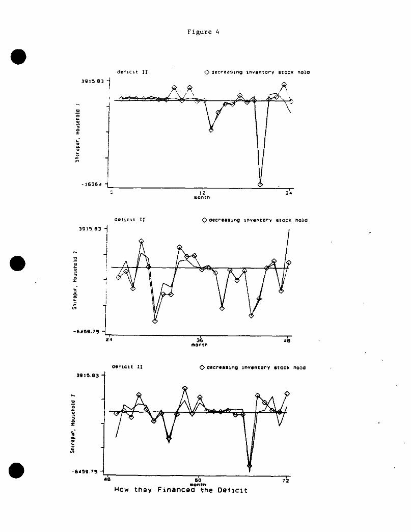
Figure 4

Defici t II

0 Decreasing Inventory stock nob

Deficit II

<>Decreasing inventory stock nolo

Def icit I I

C>Oecreasing inventory stock holD

3915.83 -

-64 59.76

60

72month

How they Financed the Deficit

O0

0082

4 -

Figure 5 •

For PmSE<6rmsel

60

Aureoal. 1-,n;raDur Kanza.monthl y Oata

Box Plots for Livestock by Village

Figure 6: O r PmSr<6*rmsec

'6 70

C)

0

Aurepall Snirapur Kanzanamontn:y data

Box Plots for Phys Assets Oy Village

•

•

III' Figure 7• rmseg

1 5

5 1

AurepalI Shirapur Kanzara

monthly oatsBox Plots for Stock Inventory by Village

Figure 8 pornm5E<2▪ rmse1

2

5 -1

•Aurepall ghsrapur Kanzara

monthly Oata

Box Plots for Borrowing by Village

O

Figure 9

•

For PMSE<2• rmsem

2 -

1.5

OAurepall Shlrapur Kenzare

monthly wits

Box Plots for Cash Holdings by Village

O

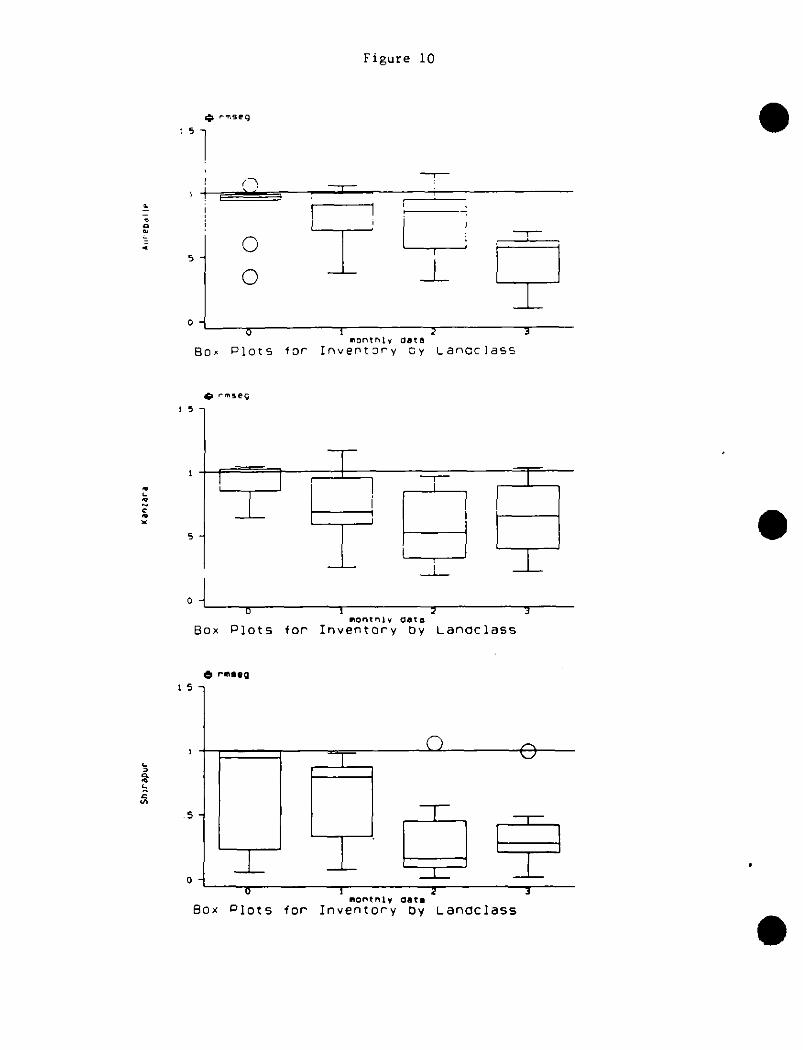
Figure 10

h.vseg

5

5 -

0 -

5 -

I

Box

0

Plots for

rmseo

1monthly

Inventory

2 3Gateoy Lanoclass

0

Is

Boxmonthly Gate

Plots for Inventory Dy Lanoclass

vb rmIsQ

Oa

5

•

00 7

3

monthly OatsBox P lots for Inventory Dy Lanoclass •

a=a

3

ala rmsem

a

Figure 11

. Box

a

0 1 3monthly data

Plots for Currency by Landclass

nmsem

00 S 2 3

monthly DataBox Plots for Currency by Landclass

rmsam

3— 0

0a

2—

o-

0

0 0 0o 1 2

monthly dataBox Plots for Currency by Landclass•

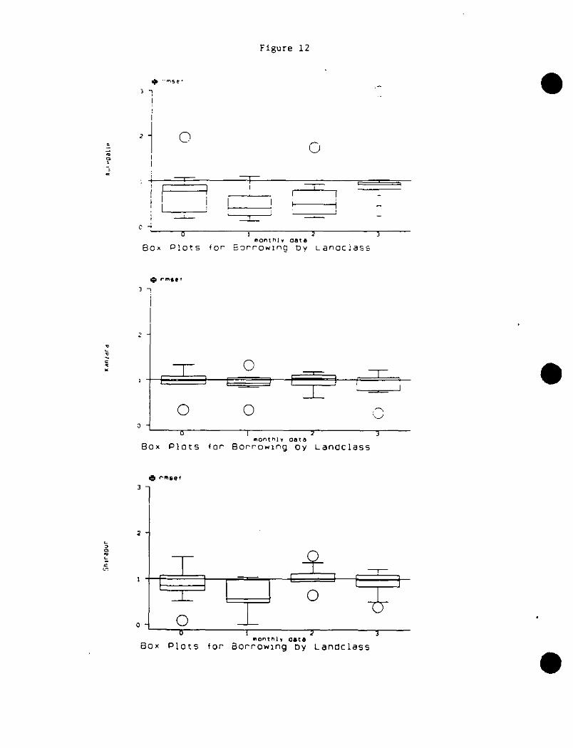
Figure 12

3•

C)0

c -;O 1 2 3

monthly oat.Box P lots for Borro w i n g Dy LanOCIaSS

• rmse.

3 -1

0

0 0O 2

3monthly on

BOx Plots f o r Borrowing oy Landclass

e rmse/

3

0

a

2

00O 2 3

monthly dataBox Plots for Borrowing Dy Landclass •

• Figure 13

rmsegm

0

O

0

•

OO

Aurepall Shirapur Kanzara

2cx Plots for Inventory and Money by Village

Figure 14

rmsefg

0

0

I0

Aureoall Shirapur Kanzara

Box Plots for Borrowing and Inventory by Village

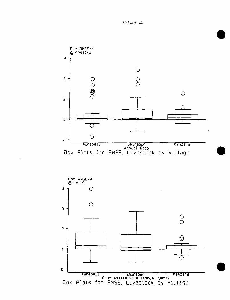
Figure 15

For AMSEcA

3-

2 -

-mseiv-1

00

0

OO

0

0Aurepall Snirapur Kanzara

Annual Data

Box Plots for PMSE, Livestock oy Village

For PmSE<4itirmsel

4 0

0

OO

Aurepall Snirapur KanzaraFrom Assets File (Annual Oata)

Box Plots for RMSE, Livestock by Village'

08

SFigure 16

For RMSE<10rmse0.1

10 7 CD

O

OO

0

8

00-

SAurepall Shirapur Kanzara

Annual Data

Box Plots for PMSE, Phys Assets

For RMSE<10rmseh

10 —

5

• 0 HAurepall Shirapur vanzara

From Assets File (Annual Data)

Box Plots for RMSE, Physical Assets by Val laoe

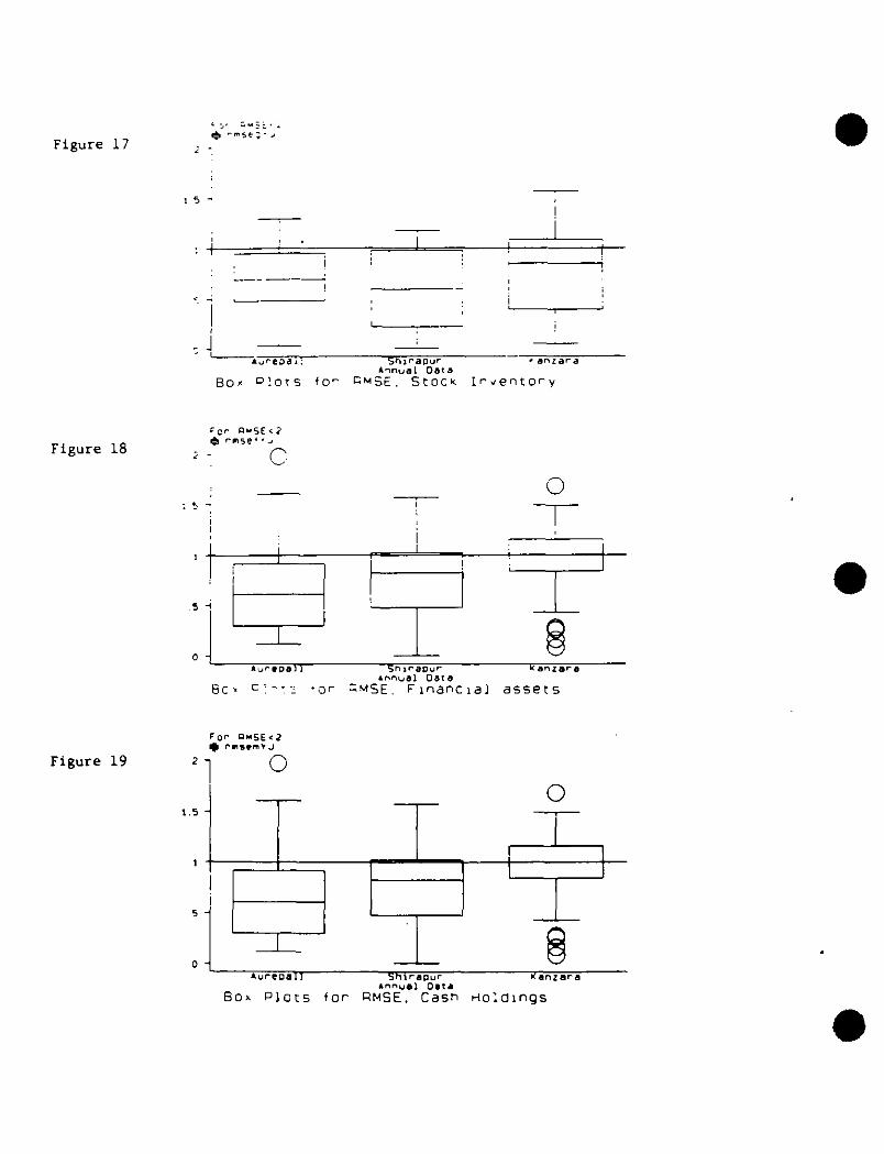
Figure 17et• ^mst;• •

15

aureoal. Sh1rapur •anzaraAnnual Data

Bog Plots fo n PmSE. Stock Irventory

Figure 18

c cr cm5E<2e rmse4o,

C

Figure 19

5 -■

•urecoa/1 Sh 1 r 8OU r aanzaraannual Data

Bc ‘ C Y s • Or : MSE. Financ i al assets

F O r clmSE<2▪ PIMSOMVJ

_ 10

•

1.5

5

0• ureca lracur Kanzara Oata

Box Plots for PMSE Casn Holaings •

76 77 7e 79 80crop year

How they Financed Deficit II

Qsum Inventory+ sum money

sum Oeftest IIQ Sum borrowing

18356.4 -

'6 77 78 79 80Cr00 veer

How they Financed Deficit II

81

-93274

Sum deficit IIQ fun borrowing

Sum Inventory+mum money

4111Figure 20

Figure 21 0000

•

75022.6

sum deficit IISue borrowing 9 eue Inventory

sum money

Figure 22 •

a•

-109326 -

76 717 78 79 80crop year

How they Financed Oeficit II

81

•

0 12Monthly Data

How they Financeo the Defic::

2 4

Sum Oeficit IIA sum borrowing

o sum inventoryq sum money

60Monthly Data

How they Financed the Deficit

34602.4 -

CaL

C

-54926.8 1

48•

72

•sum deficit II o sum Inventory

A sum borrowing o sum money

-970036 -

5:258.3

Figure 23 •

Figure 24

•49424 -

sum deficit IIA sum borrowing

o sum inventoryq sum money

a)

-56718.9 -

48 60

72Monthly Data

How they Financed the Deficit

Figure 25

•

•