Software Defect Prediction Models for Quality Improvement:
A Literature Study
Mrinal Singh Rawat1, Sanjay Kumar Dubey2
1 Department of Computer Science Engineering, MGM’s COET, Noida,
Uttar Pradesh, India
2 Department of Computer Science Engineering, Amity University, Noida,
Uttar Pradesh, India
Abstract In spite of meticulous planning, well documentation and proper
process control during software development, occurrences of
certain defects are inevitable. These software defects may lead to
degradation of the quality which might be the underlying cause
of failure. In today‟s cutting edge competition it‟s necessary to
make conscious efforts to control and minimize defects in
software engineering. However, these efforts cost money, time
and resources. This paper identifies causative factors which in
turn suggest the remedies to improve software quality and
productivity. The paper also showcases on how the various
defect prediction models are implemented resulting in reduced
magnitude of defects.
Keywords: Software Defects, Defect Prediction, Defect
Prediction, Software Quality, Machine Learning Algorithms,
Defect Density.
1. Introduction
Software metrics has been used to describe the complexity
of the program and, to estimate software development time.
“How to predict the quality of software through software
metrics, before it is being deployed” is a burning question,
triggering the substantial research efforts to uncover an
answer to this question. There are number of papers
supporting statistical models and metrics which profess to
answer the quality question. Typically, software metrics
elucidate quantitative measurements of the software
product or its specifications. Defects can be defined in a
disparate ways but are generally defined as aberration
from specifications or ardent expectations which might
lead to failures in procedure. Defect data analysis is of two
types; Classification and prediction that can be used to
extract models describing significant defect data classes or
to predict future defect trends. Classification predicts
categorical or discrete, and unordered labels, whereas
prediction models predict continuous valued functions.
Such analysis can help us for providing better
understanding of the software defect data at large.
A software defect is an error, flaw, bug, mistake, failure,
or fault in a computer program or system that may
generate an inaccurate or unexpected outcome, or
precludes the software from behaving as intended. A
project team always aspires to procreate a quality software
product with zero or little defects. High risk components
within the software project should be caught as soon as
possible, in order to enhance software quality. Software
defects always incur cost in terms of quality and time.
Moreover, identifying and rectifying defects is one of the
most time consuming and expensive software processes. It
is not practically possible to eliminate each and every
defect but reducing the magnitude of defects and their
adverse effect on the projects is achievable.
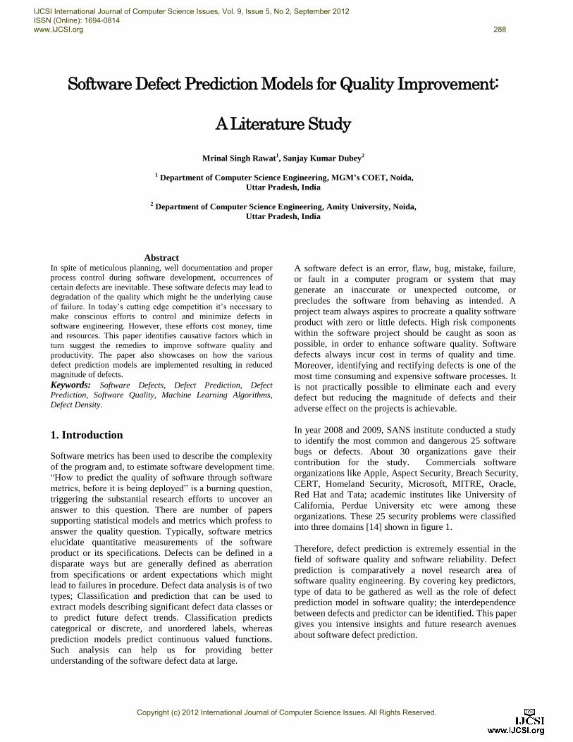
In year 2008 and 2009, SANS institute conducted a study
to identify the most common and dangerous 25 software
bugs or defects. About 30 organizations gave their
contribution for the study. Commercials software
organizations like Apple, Aspect Security, Breach Security,
CERT, Homeland Security, Microsoft, MITRE, Oracle,
Red Hat and Tata; academic institutes like University of
California, Perdue University etc were among these
organizations. These 25 security problems were classified
into three domains [14] shown in figure 1.
Therefore, defect prediction is extremely essential in the
field of software quality and software reliability. Defect
prediction is comparatively a novel research area of
software quality engineering. By covering key predictors,
type of data to be gathered as well as the role of defect
prediction model in software quality; the interdependence
between defects and predictor can be identified. This paper
gives you intensive insights and future research avenues
about software defect prediction.
IJCSI International Journal of Computer Science Issues, Vol. 9, Issue 5, No 2, September 2012 ISSN (Online): 1694-0814 www.IJCSI.org 288
Copyright (c) 2012 International Journal of Computer Science Issues. All Rights Reserved.
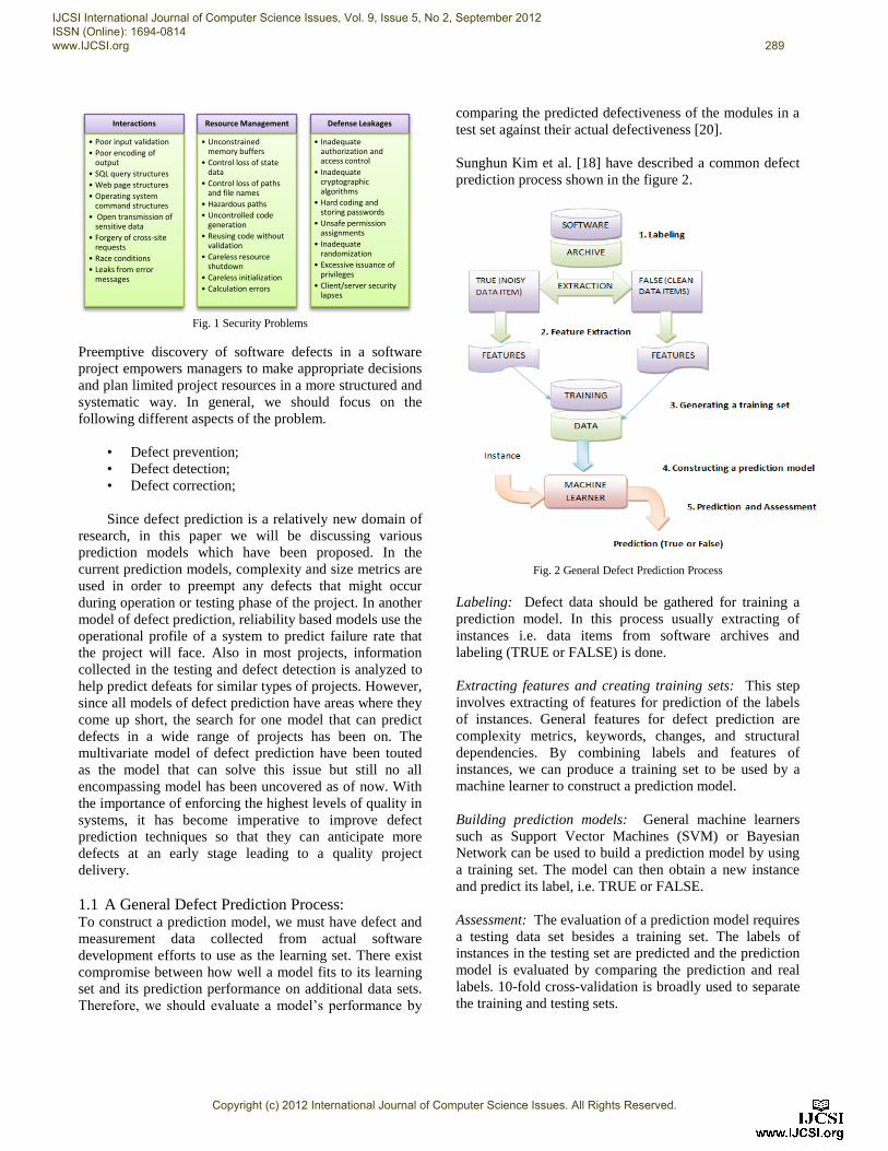
Fig. 1 Security Problems
Preemptive discovery of software defects in a software
project empowers managers to make appropriate decisions
and plan limited project resources in a more structured and
systematic way. In general, we should focus on the
following different aspects of the problem.
• Defect prevention;
• Defect detection;
• Defect correction;
Since defect prediction is a relatively new domain of
research, in this paper we will be discussing various
prediction models which have been proposed. In the
current prediction models, complexity and size metrics are
used in order to preempt any defects that might occur
during operation or testing phase of the project. In another
model of defect prediction, reliability based models use the
operational profile of a system to predict failure rate that
the project will face. Also in most projects, information
collected in the testing and defect detection is analyzed to
help predict defeats for similar types of projects. However,
since all models of defect prediction have areas where they
come up short, the search for one model that can predict
defects in a wide range of projects has been on. The
multivariate model of defect prediction have been touted
as the model that can solve this issue but still no all
encompassing model has been uncovered as of now. With
the importance of enforcing the highest levels of quality in
systems, it has become imperative to improve defect
prediction techniques so that they can anticipate more
defects at an early stage leading to a quality project
delivery.
1.1 A General Defect Prediction Process: To construct a prediction model, we must have defect and
measurement data collected from actual software
development efforts to use as the learning set. There exist
compromise between how well a model fits to its learning
set and its prediction performance on additional data sets.
Therefore, we should evaluate a model‟s performance by
comparing the predicted defectiveness of the modules in a
test set against their actual defectiveness [20].
Sunghun Kim et al. [18] have described a common defect
prediction process shown in the figure 2.
Fig. 2 General Defect Prediction Process
Labeling: Defect data should be gathered for training a
prediction model. In this process usually extracting of
instances i.e. data items from software archives and
labeling (TRUE or FALSE) is done.
Extracting features and creating training sets: This step
involves extracting of features for prediction of the labels
of instances. General features for defect prediction are
complexity metrics, keywords, changes, and structural
dependencies. By combining labels and features of
instances, we can produce a training set to be used by a
machine learner to construct a prediction model.
Building prediction models: General machine learners
such as Support Vector Machines (SVM) or Bayesian
Network can be used to build a prediction model by using
a training set. The model can then obtain a new instance
and predict its label, i.e. TRUE or FALSE.
Assessment: The evaluation of a prediction model requires
a testing data set besides a training set. The labels of
instances in the testing set are predicted and the prediction
model is evaluated by comparing the prediction and real
labels. 10-fold cross-validation is broadly used to separate
the training and testing sets.
Interactions
• Poor input validation
• Poor encoding of output
• SQL query structures
• Web page structures
• Operating system command structures
• Open transmission of sensitive data
• Forgery of cross-site requests
• Race conditions
• Leaks from error messages
Resource Management
• Unconstrained memory buffers
• Control loss of state data
• Control loss of paths and file names
• Hazardous paths
• Uncontrolled code generation
• Reusing code without validation
• Careless resource shutdown
• Careless initialization
• Calculation errors
Defense Leakages
• Inadequate authorization and access control
• Inadequate cryptographic algorithms
• Hard coding and storing passwords
• Unsafe permission assignments
• Inadequate randomization
• Excessive issuance of privileges
• Client/server security lapses
IJCSI International Journal of Computer Science Issues, Vol. 9, Issue 5, No 2, September 2012 ISSN (Online): 1694-0814 www.IJCSI.org 289
Copyright (c) 2012 International Journal of Computer Science Issues. All Rights Reserved.
2. Problem Definition
As we have discussed upon earlier, defect prediction is
vital in nature. Our prime objective is to predict defects
without overrunning the estimated cost as well as without
delaying scheduled delivery of software. However, the
main issue related to this is mainly the plethora of models
which can be used for the same. All models of defect
prediction have their own set of advantages and
disadvantages which makes it hard to understand which
fault prediction model should be used and more
importantly in what type of project. Since every project
tends to be unique, this is hard from a decision making
standpoint. However, we believe thorough model
evaluation can enable project managers to make a more
informed decision.
In our study, we will cover the popular models of defect
prediction and evaluate the pros and cons of each model
along with the situations where the models can be used.
We will evaluate the models based a varied set of criteria
depending on the model being discussed. After evaluation,
we will also include our personal observations and
interpretations on why we think certain decision models
are useful along with substantiating case studies of real
world usage wherever possible.
3. Study of Software Defect Prediction Models
3.1 Prediction Model using size and complexity
metrics
Among the popular models of defect prediction, the
approach that uses size and complexity metrics is fairly
well known. This model uses the program code as a basis
for prediction of defects. More specifically, lines of code
(LOC) are used along with the concept of complexity
model developed by McCabe. Using regression equations,
simple prediction metrics estimates can be obtained using
a dependent variable (D) defined as the sum of defects
found during testing and after 2 months post release.
Famously, Akiyama made 4 equations. We have illustrated
the equation that includes the LOC metric:
Defect (D) = 4.86 + 0.018 Lines of Code (L) (1)
Gaffney deduced above equation (1) into another
prediction equation. He argued that LOC was not language
dependent owing to optimal size for individual modules
with regards to defect density. The regression equation is
given below:
D = 4.2 + 0.0015 L4/3 (2)
The size and complexity models presume that defects are
direct function of size or defects are occurred due to
program complexity. This model ignores the underlying
casual effects of programmers and designers. They are the
human factors who actually commence the defects, so any
attribution for flawed code depends on individual(s) to
certain extent. Poor design capability or problem difficulty
may result in highly complex programs. Difficult problems
might require complex solutions and naive programmers
might create „spaghetti code‟ [6].
3.2 Machine Learning Based Models
Machine learning (ML) algorithms has demonstrated great
practical significance in resolving a wide range of
engineering problems encompassing the prediction of
failure, error, and defect-impulsions as the system software
grows to be more complex. ML algorithms are very useful
where problem domains are not well defined, human
knowledge is limited and dynamic adaption for changing
condition is needed, in order to develop efficient
algorithms. Machine learning encompasses different types
of learning such as artificial neural networks (ANN),
concept learning (CL), Bayesian belief networks (BBN),
reinforcement learning (RL), genetic algorithms (GA) and
genetic programming (GP), instance-based learning (IBL),
decision trees (DT), inductive logic programming (ILP),
and analytical learning (AL)[3].
G. John, P. Langley [4] employed RF method for
prediction of faulty modules with NASA data sets.
Prediction of software quality was introduced by
Khoshgaftaar et al. [5] by using artificial neural network.
In this model they classified modules as fault prone or non
fault prone, using large telecommunication software
system. They compared their end results with another non–
parametric model achieved from discriminant method.
Fenton et al. [6] suggested the use of Bayesian belief
networks (BBN) for the prediction of faulty software
modules. Elish et al. [7] recommended the use of support
vector machines for predicting defected modules with
context of NASA data sets. This model compares its
prediction performance with other statistical and machine
learning models. We have discussed few models in detail
to enhance the understanding of Machine learning based
prediction models.
3.2.1 The Probabilistic Model for Defect Prediction
using Bayesian Belief Network
Fenton, Krause and Neil [6] proposed a probabilistic
model for defect prediction. They recommended a holistic
model rather than a single issue (for e.g. size, or
complexity, or testing metrics, or process quality data)
model, by combining the different factors of casual
IJCSI International Journal of Computer Science Issues, Vol. 9, Issue 5, No 2, September 2012 ISSN (Online): 1694-0814 www.IJCSI.org 290
Copyright (c) 2012 International Journal of Computer Science Issues. All Rights Reserved.
evidence in order to successful defect prediction. The
model uses Bayesian Belief Network (BBN) as the
suitable practice for representation of this evidence. The
Bayesian approach causes statistical conclusion to be
improved by expert judgment in those parts of a problem
sphere where empirical data is scattered. Additionally, the
causal or influence organization of the model better
reflects the series of real world events and relations than
any other practice.
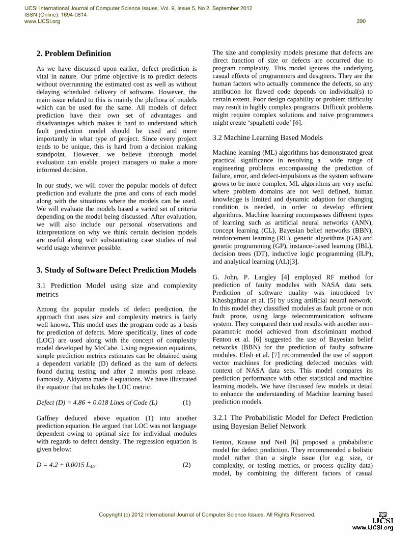
BBN can be exploited to support effective decision
making for SPI (Software Process Improvement), by
executing the following steps.
Fig. 3 Bayesian Approach
A BBN represents the joint probability distribution
for a set of variables. This is achieved by defining Directed
acyclic graph (DAG) and Conditional probability tables A
BBN can be employed to deduce the probability
distribution for a target variable (e.g., “Defects Detected”),
which indicates the probability that the variable will
obtain on each of its possible values (e.g., “very
low”, “low”, “average”, “high”, or “very high” for the
variable “Defects Detected”) given the observed values
of the other variables [8, 9].
N. Fenton, M. Neil and D. Marquez [17] reviewed the use
of Bayesian networks to overcome impediments of using
BN‟s for predicting software defects and software quality.
BN tools and algorithms suffered from „Achilles‟ heel.
This compelled modelers to predefine discretization
intervals in advance and resulted in inadequate predictions
for large set of data. To improve this „dynamic
discretization‟ algorithm was used. This algorithm exploits
entropy error as the basis for approximation allowing more
accuracy.
3.2.1 The Probabilistic Model for Defect Prediction
using Bayesian Belief Network
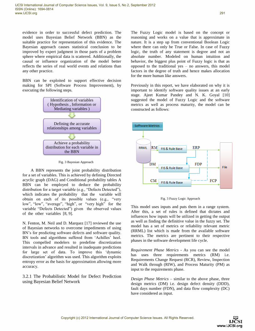
The Fuzzy Logic model is based on the concept or
reasoning and works on a value that is approximate in
nature. It is a step up from conventional Boolean Logic
where there can only be True or False. In case of Fuzzy
logic, the truth of any statement is degree and not an
absolute number. Modeled on human intuition and
behavior, the biggest plus point of Fuzzy logic is that as
opposed to the traditional yes – no answers, this model
factors in the degree of truth and hence makes allocation
for the more human like answers.
Previously in this report, we have elaborated on why it is
important to identify software quality issues at an early
stage. Ajeet Kumar Pandey and N. K. Goyal [10]
suggested the model of Fuzzy Logic and the software
metrics as well as process maturity, the model can be
constructed as follows:
Fig. 3 Fuzzy Logic Approach
This model uses inputs and puts them in a range system.
After this, a set of rules is defined that dictates and
influences how inputs will be utilized in getting the output
as well as finding the definitive value in the fuzzy set. The
model has a set of metrics or reliability relevant metric
(RRML) list which is made from the available software
metrics. The metrics are pertinent to their respective
phases in the software development life cycle.
Requirement Phase Metrics - As you can see the model
has uses three requirements metrics (RM) i.e.
Requirements Change Request (RCR), Review, Inspection
and Walk through (RIW), and Process Maturity (PM) as
input to the requirements phase.
Design Phase Metrics – similar to the above phase, three
design metrics (DM) i.e. design defect density (DDD),
fault days number (FDN), and data flow complexity (DC)
have considered as input.
Identification of variables ( Hypothesis , Information or
Mediating variables )
Defining the accurate relationships among variables
Achieve a probability distribution for each variable in
the BBN
IJCSI International Journal of Computer Science Issues, Vol. 9, Issue 5, No 2, September 2012 ISSN (Online): 1694-0814 www.IJCSI.org 291
Copyright (c) 2012 International Journal of Computer Science Issues. All Rights Reserved.
Coding Phase Metrics – In this phase, two coding metrics
(CM) such as code defect density (CDD) and cyclomatic
complexity (CC) have been taken as input at coding phase.
The outputs of the model will be the number of faults at
the end of Requirements Phase (FRP), number of Faults at
the end of Design Phase (FDP), and number of Faults at
the end of Coding Phase (FCP).
3.2.3 Defect Prediction Models Based on Genetic
Algorithms
Genetic Algorithms is an approach to machine learning
which behaves similarly to the human gene and the
Darwinian theory of natural selection. It is a part of the
Evolutionary Algorithms which generate solutions based
on the techniques more commonly found in nature like
mutation, selection, crossover etc.
Genetic Algorithms are implemented beginning with an
individual population that is usually represented in the
form of trees. A possible solution is represented by each
tree or say chromosome in this case. Nodes on the tree
signify particular traits that relates to the problem for
which the solution is being searched. Collectively, the set
of potential solutions to the problem is (represented by the
chromosomes) as known as the population.
Where genetic algorithms come into place is when you
need to solve problems which can have many solutions.
Here, genetic algorithms are being used to cluster the
classes defined as per object oriented metrics into
subsystems or commonly known as components of
software. As elaborated earlier, genetic algorithm uses an
approach akin to Charles Darwin‟s “Survival of the
Fittest” or natural selection. The reason this approach is
being considered is because the large solutions set which
provide a number of possible solutions to a problem.
When applying a genetic algorithm to a problem, there are
a few implications which are made. The same are as
follows
a) There must be a fitness function present for the
evaluation of weather a solution is a possible one
or not
b) Whenever there is a solution found, there should
a representation of it made by a chromosome.
c) Whichever genetic operators will be applied must
be established
Additionally the definition of a solution in this case would
be one which would be both complete as well as valid. In
terms of a representation, there is the assumption that the
possible solutions have been encoded in the solutions
space.
How do Genetic Algorithms work?
In the beginning, the Genetic Algorithms start with a large
population. In that population, each individual represents a
plausible solution to the problem. These individuals in the
population are then encoded in a binary string that is called
a chromosome. After that, the group of the individuals will
compete so that they can reproduce and then formulate the
next generation. However, there is a function called the
fitness function that determines which of the competing
individuals will gain the right to reproduce. Having the
fitness function in place makes sure that only the best
individuals of the population will be able to carry over
their offspring into the next generation. The next
generation is formed by the following activities taking
place.
a) Reproduction – reproduction process takes place
when two chromosomes exchange a portion of
their code to form the new individuals. The
crossover points (where the bits of the code will
exchange) are selected by random (for a simple
version of the algorithm). At the crossover point,
the chromosomes exchange the data keeping the
original data up to that point.
b) Mutations – this comes in to introduce variation
in the next generation which prevents the
reaching of local minima. Whereas crossover
alters the genes after a randomly selected
crossover point between 2 chromosomes,
mutation selects on node in the tree of one
chromosome and changes the genetic material.
This process repeats itself until there is a perfect solution
set reached (optimal fitness level). However, there are
occasions when this does not happen. In such cases, the
program terminates after a set of iterations. The iterations
of the proceeds are also known as generations.
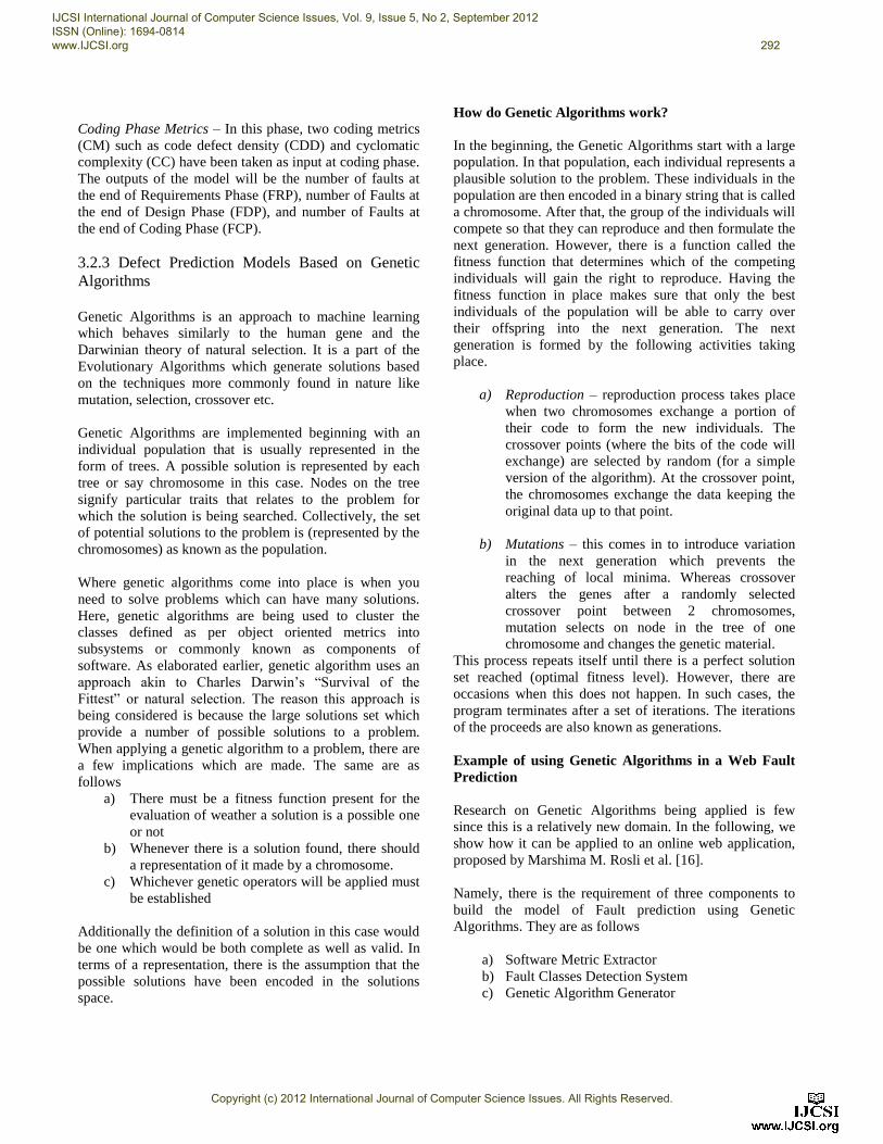
Example of using Genetic Algorithms in a Web Fault
Prediction
Research on Genetic Algorithms being applied is few
since this is a relatively new domain. In the following, we
show how it can be applied to an online web application,
proposed by Marshima M. Rosli et al. [16].
Namely, there is the requirement of three components to
build the model of Fault prediction using Genetic
Algorithms. They are as follows
a) Software Metric Extractor
b) Fault Classes Detection System
c) Genetic Algorithm Generator
IJCSI International Journal of Computer Science Issues, Vol. 9, Issue 5, No 2, September 2012 ISSN (Online): 1694-0814 www.IJCSI.org 292
Copyright (c) 2012 International Journal of Computer Science Issues. All Rights Reserved.
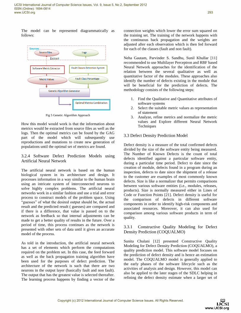
The model can be represented diagrammatically as
follows:
Fig 5 Genetic Algorithm Approach
How this model would work is that the information about
metrics would be extracted from source files as well as the
logs. Then the optimal metrics can be found by the GAG
part of the model which will subsequently use
reproductions and mutations to create new generation of
populations until the optimal set of metrics are found.
3.2.4 Software Defect Prediction Models using
Artificial Neural Network
The artificial neural network is based on the human
biological system in its architecture and design. It
processes information in a way similar to the human brain
using an intricate system of interconnected neurons to
solve highly complex problems. The artificial neural
networks work in a similar fashion and use a trial and error
process to construct models of the problem space. Using
“guesses” of what the desired output should be, the actual
result and the predicted result ( guesses) are compared and
if there is a difference, that value is passed on to the
network as feedback so that internal adjustments can be
made to get a better quality of results in the future. Over a
period of time, this process continues as the network is
presented with other sets of data until it gives an accurate
model of the process.
As told in the introduction, the artificial neural network
has a set of elements which perform the computations
required on the problem set. In this case, the feed forward
as well as the back propagation training algorithm have
been used for the purposes of defect prediction. The
architecture of the network is such that there are two
neurons in the output layer (basically fault and non fault).
The output that has the greatest value is selected thereafter.
The learning process happens by finding a vector of the
connection weights which lower the error sum squared on
the training set. The training of the network happens with
the continuous back propagation and the weights are
adjusted after each observation which is then fed forward
for each of the classes (fault and non fault).
Neha Gautam, Parvinder S. Sandhu, Sunil Khullar [11]
recommended to use Multilayer Perceptron and RBF based
Neural Network approaches for the identification of the
relation between the several qualitative as well as
quantitative factor of the modules. These approaches also
identify the number of defects existing in the module that
will be beneficial for the prediction of defects. The
methodology consists of the following steps:
1. Find the Qualitative and Quantitative attributes of
software systems
2. Select the suitable metric values as representation
of statement
3. Analyze, refine metrics and normalize the metric
values and Explore different Neural Network
Techniques
3.3 Defect Density Prediction Model
Defect density is a measure of the total confirmed defects
divided by the size of the software entity being measured.
The Number of Known Defects is the count of total
defects identified against a particular software entity,
during a particular time period. Defect to date since the
creation of module, defects found in a program during an
inspection, defects to date since the shipment of a release
to the customer are examples of most commonly known
defects. Size is like a normalizer that permits comparisons
between various software entities (i.e., modules, releases,
products). Size is normally measured either in Lines of
Code or Function Points [21]. Defect density is useful for
the comparison of defects in different software
components in order to identify high-risk components and
associated resources. Moreover, it can also used for
comparison among various software products in term of
quality.
3.3.1 Constructive Quality Modeling for Defect
Density Prediction (COQUALMO)
Sunita Chulani [12] presented Constructive Quality
Modeling for Defect Density Prediction (COQUALMO), a
quality prediction model. This software model focuses on
the prediction of defect density and is hence an estimation
model. The COQUALMO model is generally applied to
the early phases of the software lifecycle such as the
activities of analysis and design. However, this model can
also be applied to the later stages of the SDLC helping in
refining the defect density estimate when a larger set of
IJCSI International Journal of Computer Science Issues, Vol. 9, Issue 5, No 2, September 2012 ISSN (Online): 1694-0814 www.IJCSI.org 293
Copyright (c) 2012 International Journal of Computer Science Issues. All Rights Reserved.
information is available. The COQUALMO model enables
project managers to get an estimate with relation to metrics
like shipping time as well as the payoffs for investing in
quality as well as a better understanding of the interactions
involved with respect to quality strategies.
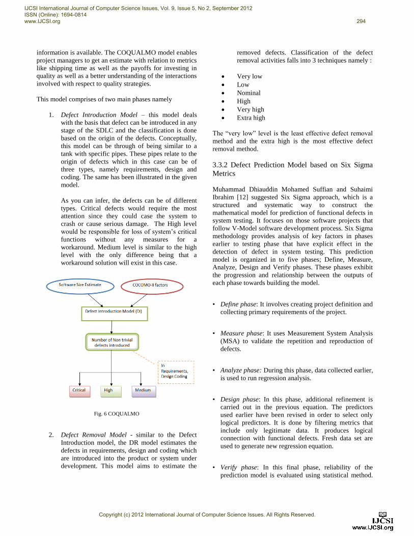
This model comprises of two main phases namely
1. Defect Introduction Model – this model deals
with the basis that defect can be introduced in any
stage of the SDLC and the classification is done
based on the origin of the defects. Conceptually,
this model can be through of being similar to a
tank with specific pipes. These pipes relate to the
origin of defects which in this case can be of
three types, namely requirements, design and
coding. The same has been illustrated in the given
model.
As you can infer, the defects can be of different
types. Critical defects would require the most
attention since they could case the system to
crash or cause serious damage. The High level
would be responsible for loss of system‟s critical
functions without any measures for a
workaround. Medium level is similar to the high
level with the only difference being that a
workaround solution will exist in this case.
Fig. 6 COQUALMO
2. Defect Removal Model - similar to the Defect
Introduction model, the DR model estimates the
defects in requirements, design and coding which
are introduced into the product or system under
development. This model aims to estimate the
removed defects. Classification of the defect
removal activities falls into 3 techniques namely :
Very low
Low
Nominal
High
Very high
Extra high
The “very low” level is the least effective defect removal
method and the extra high is the most effective defect
removal method.
3.3.2 Defect Prediction Model based on Six Sigma
Metrics
Muhammad Dhiauddin Mohamed Suffian and Suhaimi
Ibrahim [12] suggested Six Sigma approach, which is a
structured and systematic way to construct the
mathematical model for prediction of functional defects in
system testing. It focuses on those software projects that
follow V-Model software development process. Six Sigma
methodology provides analysis of key factors in phases
earlier to testing phase that have explicit effect in the
detection of defect in system testing. This prediction
model is organized in to five phases; Define, Measure,
Analyze, Design and Verify phases. These phases exhibit
the progression and relationship between the outputs of
each phase towards building the model.
• Define phase: It involves creating project definition and
collecting primary requirements of the project.
• Measure phase: It uses Measurement System Analysis
(MSA) to validate the repetition and reproduction of
defects.
• Analyze phase: During this phase, data collected earlier,
is used to run regression analysis.
• Design phase: In this phase, additional refinement is
carried out in the previous equation. The predictors
used earlier have been revised in order to select only
logical predictors. It is done by filtering metrics that
include only legitimate data. It produces logical
connection with functional defects. Fresh data set are
used to generate new regression equation.
• Verify phase: In this final phase, reliability of the
prediction model is evaluated using statistical method.
IJCSI International Journal of Computer Science Issues, Vol. 9, Issue 5, No 2, September 2012 ISSN (Online): 1694-0814 www.IJCSI.org 294
Copyright (c) 2012 International Journal of Computer Science Issues. All Rights Reserved.
Capability flow-up and scorecard are performed to
ensure customer requirements are fulfilled.
The Design for Six Sigma (DfSS) methodology also
provides a Control plan that guides on subsequent action
when the genuine functional defects discovered do not
occur within the range of prediction interval. The Six
Sigma method of building defect prediction models is a
good fit of software defect prediction. The processes and
methodologies proposed in Six Sigma provide ample
opportunities to formulate a clear outline of issues to be
addressed, the data collection as well as measurement
along with model generation, construction and validation.
Equations formulated by the model give a good idea on
what could be the possible factors which contribute to
defects.
4. Conclusions
Prediction is the task of predicting continuous or ordered
values for given input. However, as we have seen, some
classification techniques such as Bayesian belief networks,
neural network and genetic algorithms can be adapted for
prediction. Training a classifier or predictor is not enough;
we would like an estimate of how accurately the classifier
can predict the deviating behavior of future defects, that is,
future defect data on which the classifier has not been
trained. We have observed various methods to construct
more than one classifier (or predictor) and now we want to
estimate their accuracy. We can use Predictor error
measures in techniques for accuracy estimation, such as
the holdout, random sub sampling, k-fold cross-validation,
and bootstrap methods.
Software defect prediction is the process of tracing
defective components in software prior to the start of
testing phase. Occurrence of defects is inevitable, but we
should try to limit these defects to minimum count. Defect
prediction leads to reduced development time, cost,
reduced rework effort, increased customer satisfaction and
more reliable software. Therefore, defect prediction
practices are important to achieve software quality and to
learn from past mistakes. Size or complexity measures are
simple regression models, which normally assume simple
relationship between defects and program complexity.
These models are not subjected to the controlled statistical
testing required to set up a causal relationship. Fenton and
Neil advocate that these models fall short to take account
of all the causal or explanatory variables necessitated in
order to construct the models generalizable. They
presented probabilistic model based on Bayesian belief
networks to overcome this problem.
Furthermore, we have presented the use of various
machine learning techniques for the software fault
prediction problem. The unfussiness, ease in model
calibration, user acceptance and prediction accuracy of
these quality estimation techniques demonstrate its
practical and applicative magnetism. These modeling
systems can be used to achieve timely fault predictions for
software components presently under development,
providing valuable insights into their quality. The software
quality assurance team can then utilize the predictions to
use available resources for obtaining cost effective
reliability enhancements.
There are number of software defect prediction models
available but in our study we have arrived on this
conclusion that these models heavily depends on the
nature ,volume of the defect data and accuracy of classifier
and predictors. Most of the researches were carried out
with the help of NASA defect data sets. We would like to
express gratitude to the NASA MDP organization for
making their defect data sets publicly available.
References [1] Clark, B. and Zubrow, D., “How Good Is the Software: A
Review of Defect Prediction Techniques”, Software
Engineering Institute, SEPG 2002 Conference.
[2] N. Fenton and M. Neil “A Critique of Software Defect
Prediction Research”, IEEE Trans. Software Eng., 25, No.5,
1999.
[3] Du Zhang, “Applying Machine Learning Algorithms in
Software Development” The Proceedings of 2000 Monterey
Workshop on Modeling Software System Structures, Santa
Margherita Ligure, Italy, pp. 275-285.
[4] L. Guo, Y. Ma, B. Cukic, H. Singh, “Robust prediction of
fault proneness by random forests,” In: Proceedings of the
15th International Symposium on Software Reliability
Engineering (ISSRE‟04), pp. 417–428, 2004.
[5] T.M. Khoshgaftaar, E.D. Allen, J.P, Hudepohl, S.J. Aud,
Application of neural networks to software quality modeling
of a very large telecommunications system,” IEEE
Transactions on Neural Networks, vol. 8, no. 4, pp. 902-
909, 1997.
[6] Norman Fenton, Paul Krause and Martin Neil, “A
Probabilistic Model for Software Defect Prediction”, IEEE
Transactions on Software Engineering, 2001.
[7] K. Elish, M. Elish, “Predicting defect-prone software
modules using support vector machines,” Journal of System
and Software, vol. 81, pp. 649-660.
[8] T. Mitchell, Machine Learning, McGraw-Hill, 1997.
[9] F.V. Jensen, “An Introduction to Bayesian Networks”,
Springer, 1996.
[10] Ajeet Kumar Pandey & N. K. Goyal, “A Fuzzy Model for
Early Software Fault Prediction Using Process Maturity and
Software Metrics” International Journal of Electronics
Engineering, 1(2), 2009, pp. 239-245.
[11] Parvinder S. Sandhu, Satish Kumar Dhiman, Anmol Goyal,
“A Genetic Algorithm Based Classification Approach for
Finding Fault Prone Classes”, World Academy of Science,
Engineering and Technology, 2009.
IJCSI International Journal of Computer Science Issues, Vol. 9, Issue 5, No 2, September 2012 ISSN (Online): 1694-0814 www.IJCSI.org 295
Copyright (c) 2012 International Journal of Computer Science Issues. All Rights Reserved.
[12] Sunita Chulani, “Constructive Quality Modeling for Defect
Density Prediction: COQUALMO”, IBM Research, Center
for Software Engineering, 1999.
[13] Muhammad Dhiauddin Mohamed Suffian, Suhaimi Ibrahim,
“A Prediction Model for Functional Defects in System
Testing Using Six Sigma”, ARPN Journal of Systems and
Software, Vol.1 No.6, pp.219-224, 2011.
[14] Software Engineering Best Practices: Lessons from
Successful Projects in the Top Companies, the McGraw-Hill
Companies, 2010, ISBN: 9780071621618.
[15] Sultan H. Aljahdali, Mohammed E. El-Telbany, “Software
Reliability Prediction Using Multi-Objective Genetic
Algorithm” IEEE, 2009.
[16] Marshima M. Rosli, Noor Hasimah Ibrahim Teo, Nor
Shahida M. Yusop and N. Shahriman Mohamad ,“Fault
Prediction Model for Web Application Using Genetic
Algorithm”, International Conference on Computer and
Software Modeling IPCSIT vol.14 (2011) IACSIT Press,
Singapore.
[17] N Fenton, M Neil and D Marquez, “Using Bayesian
Networks to Predict Software Defects and Reliability”,
Proceeding of the Institution of Mechanical Engineers, Vol.
222 Part O: Journal of Risk and Reliability, 2008.
[18] Sunghun Kim, Hongyu Zhang, Rongxin Wu and Liang
Gong, “Dealing with Noise in Defect Prediction”, CSE‟11,
Waikiki, Honolulu, HI, USA, ACM 978-1-4503-0445-
0/11/05, 2011.
[19] Yogesh Singh, Arvinder Kaur, Ruchika Malhotra, “Software
Fault Proneness Prediction Using Support Vector
Machines”, Proceedings of the World Congress on
Engineering 2009 Vol I WCE 2009, July 1 - 3, 2009,
London, U.K.
[20] A. Güneş Koru and Hongfang Liu ,“Building Effective
Defect-Prediction Models in Practice” IEEE, Vol. 22, No. 6
November/December 2005.
[21] Linda Westfall, Defect Density
http://www.westfallteam.com/Papers/defect_density.pdf.
[22] Yue Jiang & Bojan Cukic & Yan Ma ,“Techniques for
evaluating fault prediction models” , Journal Empirical
Software Engineering ,Volume 13, Issue 5, pp 561 – 595,
October 2008 .
[23] Tibor Gyimothy, Rudolf Ferenc, and Istvan Siket
,“Empirical Validation of Object-Oriented Metrics on Open
Source Software for Fault Prediction”, IEEE Transactions
on Software Engineering, Vol. 31,No. 10,October 2005
Ms. Mrinal Singh Rawat is Assistant Professor in the Department of Computer Science and Engineering in MGM‘s COET, Noida, UP, INDIA. Her Research activities are based on Software Engineering, Artificial Intelligence and Data Mining. She is pursuing her M.Tech in Computer Science and Engineering from Amity University.
Mr. Sanjay Kumar Dubey is working as Assistant Professor in Department of Computer Science and Engineering in Amity University Noida, UP, INDIA. His Research area includes Software Engineering and Usability Engineering. He is pursuing his Ph.D in Computer Science and Engineering from Amity University.
IJCSI International Journal of Computer Science Issues, Vol. 9, Issue 5, No 2, September 2012 ISSN (Online): 1694-0814 www.IJCSI.org 296
Copyright (c) 2012 International Journal of Computer Science Issues. All Rights Reserved.
Recommended